Computations of spectral radii on G-spacespi.math.cornell.edu/~lsc/sunada.pdf · Contemporary Mathematics Computations of spectral radii on G-spaces Laurent Saloﬀ-Coste and Wolfgang

Contemporary Mathematics

Computations of spectral radii on G-spaces

Laurent Saloff-Coste and Wolfgang Woess

Dedicated to Professor Toshikazu Sunada on the occasion of his 60th birthday

Abstract. In previous work, we have developped methods to compute normsand spectral radii of transition operators on proper metric spaces. The oper-ators are assumed to be invariant under a locally compact, amenable groupwhich acts with compact quotient.

Here, we present several further applications of those methods. The firstconcerns a generalization of an identity of Hardy, Littlewood and Polya. Thesecond is a detailed study of a class of diffusion operators on a homogeneoustree, seen as a 1-complex. Finally, we investigate the implications of ourmethod for computing spectral radii of convolution operators on general locallycompact groups and Lie groups.

1. Introduction

In a series of papers [13], [14], [15] based on ideas introduced by Soardi andWoess [18] and Salvatori [16], we have developed tools to compute the norms and/orspectral radii of Markov operators that are invariant under the left action of a groupwhen the action is either transitive or almost transitive (i.e has a compact factorspace). In [13], [14], we where concerned with countable homogeneous spaces. Atypical example is given by the simple random walk on the vertex set of the (r+1)-regular tree T = Tr. For each vertex v, set K(v, w) = 1/(r + 1) if w is a neighborof v, and K(v, w) = 0 otherwise. There are many groups G that act transitivelyon the vertex set of the tree and such that K(gv, gw) = K(v, w) for all g ∈ G.One such group is the group of those isometries of the tree that fix one end. SeeFigure 1 below in Section 4. This group is amenable and non-unimodular. Thesetwo properties lead to an easy computation of the norms σp(K) and spectral radiiρp(K) of the operator K acting on Lp(T), 1 ≤ p ≤ ∞ (the reference measure hereis the counting measure).

In [15], the theory developed in [14] is extended to general locally compactstate spaces. The purpose of the present paper is to illustrate some of the resultsof [15] with concrete applications and examples. In Section 2, we briefly introduce

1991 Mathematics Subject Classification. Primary 43A85; Secondary 47A30, 60J60 .Key words and phrases. amenable locally compact group, G-space, transition operator, con-

volution, modular function, Laplace operator, tree.

c©0000 (copyright holder)

1

2 LAURENT SALOFF-COSTE AND WOLFGANG WOESS

the general framework and recall the relevant results of [15], in particular themain tool, Theorem 2.1. In the short Section 3, we explain a generalization ofTheorem 2.1 and its relation to an identity of Hardy, Littlewood and Polya [7]plus extensions of the latter. The remaining Sections are devoted to two classesof examples: Section 4 deals with diffusion operators with constant coefficients ona regular tree, seen as a 1-complex where each edge is a copy of the unit interval.Section 5 links our results with classic harmonic analysis by looking at convolutionoperators on semisimple and other Lie groups, as well as general locally compactgroups, not always necessarily connected.

2. Theoretical background

The notation used in this section follows closely that of [15].

2.A. Invariant measures. Let X be a metric space whose closed balls arecompact (i.e., a proper metric space). Let G be a locally compact group which actsproperly on X . Let I be the quotient space I = G\X (we use this notation becausewe will always think of G acting on X from the left). For each s ∈ I, we denote byXs the corresponding equivalence class in X so that

X =⋃

s∈I

Xs .

Each orbit Xs is a G-homogeneous space, and for each x ∈ Xs we have Xs∼= G/Gx

where Gx ⊂ G is the stabilizer of x. By properness of the action, Gx is compact.On each Xs there is, up to a multiplicative constant, a unique G-invariant measuredXs

. Given a fixed left Haar measure dG on G and a fixed G-invariant measure dXs

on each Xs , we obtain for each x ∈ X a specific Haar measure dGxon the stabilizer

Gx so that

(1)

∫

G

F (g) dGg =

∫

Xs

(∫

Gx

F (gx,yh) dGxh

)dXs

y .

Let

(2) γ(x) = |Gx|denote the total mass of the compact group Gx under dGx

. There is a slight abuseof notation here because the precise normalization of the measure dGx

depends onthe point x. In particular, for two points x 6= z in X , we can have |Gx| 6= |Gz | evenif Gx = Gz as subgroups of G.

We now have to face the question of the choice of a G-invariant measure onX and its decomposition over I. Indeed, as soon as I is not a singleton, thereare non-equivalent G-invariant measures on G. Moreover, there are many ways todecompose a given G-invariant measure over the quotient space I.

Let dX be a G-invariant measure on X . Let C00(X) be the space of all con-tinuous compactly supported functions on X . Assume that the factor space I isequipped with a measure dλ, that each orbitXs is equipped with a fixed G-invariantmeasure dXs

, and that the measure dXx decomposes as follows:

(a) For any f ∈ C00(X) and its restriction fs to Xs ,

(3)

∫

X

f(x) dXx =

∫

I

∫

Xs

fs(x) dXsx dλ(s) .

COMPUTATIONS OF SPECTRAL RADII ON G-SPACES 3

(b) The function γ : x 7→ γ(x) = |Gx| induced by the choice of the G-invariantmeasures dXs

is continuous on X .

We call such a decomposition of dX a continuous decomposition. See [15, §9] for aproof of the existence of such a decomposition for any G-invariant measure on X .

2.B. Invariant operators. On X as above, consider a non-negative kernelk(x, y) and the associated operator

Kf(x) =

∫

X

k(x, y)f(y) dXy .

This definition makes sense, very generally, at least for non-negative functions f .We make the crucial hypothesis that K is G-invariant, that is, for all x, y ∈ X andg ∈ G,

k(gx, gy) = k(x, y) .

We do not assume here that k is a Markov kernel although it will be Markovian inmost of our applications. Our aim is to compute the norms

σp(K) = sup{‖Kf‖p : f ∈ Lp(X, dx), f ≥ 0, ‖f‖p ≤ 1}and spectral radii

ρp(K) = limn→∞

σp(Kn)1/n ,

where 1 ≤ p ≤ ∞ and (for p 6= ∞)

‖f‖p =

(∫

X

|f(x)|p dXx

)1/p

.

Since k is non-negative, this makes sense without further assumption if we admitthe possibility that those quantities are infinite.

For each s, t ∈ I and each p ∈ [1,∞], set

(4) ap(s, t) = ap[K](s, t) =

∫

Xt

(γ(y)

γ(xs)

)1/p

k(xs, y) dXty

where xs is a fixed reference point in Xs and the function γ is defined by (2). ByG-invariance, one can check that ap(s, t) does not depend on the choice of xs in Xs ,see [15, Theorem 2.12]. The crucial fact here is that for any g ∈ G and x ∈ X , wehave (see [15, Lemma 2.6])

(5) ∆(g) = γ(x)/γ(gx) ,

where ∆(g) is the modular function of G defined by

∆(g)

∫

G

f(hg) dGh =

∫

G

f(h) dGh .

Denote by Ap = Ap[K] the operator on Lp(I, dλ) defined by

(6) Apf(s) =

∫

I

ap(s, t)f(t) dλ(t).

We denote by σp(A) (resp. ρp(A)) the norm (resp. spectral radius) of A acting onLp(I, dλ). The result whose application we want to illustrate in this paper is thefollowing.


Theorem 2.1. Assume that G is amenable and that we have a continuousdecomposition of dX over I as in (3). Then

σp(K) = σp(Ap[K]) and ρp(K) = ρp(Ap[K]) .

When I is compact, this is contained in [15, Theorem 5.3]. The proof goesthrough also when I is non-compact (see also [14] for the case whenX is countable);compactness of I is needed in [15] for the converse, namely, for deducing amenabilityfrom the above equalities.

Remark 2.2. (a) Denote by K∗ the operator with kernel k∗(x, y) = k(y, x)(i.e., the “formal” adjoint of K). Then, for any 1 ≤ p, q ≤ ∞ with 1/p+ 1/q = 1,we have aq[K

∗](s, t) = ap[K](t, s), in accordance with the fact that σq(K∗) = σp(K)

and ρq(K∗) = ρp(K).

(b) Let K1,K2 be two operators with kernels k1, k2 as above. Then, for any 1 ≤p ≤ ∞, we have

ap[K1K2](s, s′) =

∫

I

ap[K1](s, t)ap[K2](t, s′) dλ(t),

that is,

(7) Ap[K1K2] = Ap[K1]Ap[K2].

3. A generalization, and an identity of Hardy, Littlewood and Polya

Suppose we want to compute the norms and spectral radii of K as above but onLp(X, dµ) with dµ(x) = m(x) dXx , where m is a positive and measurable function.Here, we assume furthermore that there is a function c(·) on G such that

(8) m(x)/m(gx) = c(g)

for all x ∈ X, g ∈ G. A simple argument, using the bijective isometry from Lp(X,µ)to Lp(X, dX) given by f 7→ m−1/pf , shows that the norm σp(K,µ) and the spectralradius ρp(K,µ) of K acting on Lp(X,µ) satisfy

σp(K,µ) = σp(Kp) and ρp(K,µ) = ρp(Kp) ,

where Kp denotes the operator with kernel(m(x)/m(y)

)1/pk(x, y)

acting on Lp(X, dX). Under the hypothesis (8), the kernel of Kp is invariant underthe action of G, which is assumed to be amenable. Theorem 2.1 applies to Kp andgives the following result.

Theorem 3.1. Let G, X, I, dX and λ be as in sections 2A–B. Assume that Gis amenable, and that the G-invariant measure dX has a continuous decompositionover (I, λ) as in (3). Let k be a non-negative G-invariant kernel on X, and let µbe a measure on X whose density with respect to dX is positive and satisfies (8).

Then the associated integral operator K acting on Lp(X, dµ) satisfies

(9) σp(K,µ) = σp(Ap,µ[K]) and ρp(K,µ) = ρp(Ap,µ[K]) ,

where

Ap,µ[K](s, t) =

∫

Xt

(γ(y)m(xs)

γ(xs)m(y)

)1/p

k(xs, y) dXty .


Above, xs is again a fixed reference point in Xs, and γ(·) is defined by (2).Let us connect (9) to a well known and useful identity of Hardy, Littlewood and

Polya [7]. On (0,∞), consider a non-negative kernel k(x, y) satisfying k(tx, ty) =t−1k(x, y), i.e., homogeneous of degree −1. Then that identity says that the oper-ator Kf(x) =

∫∞

0k(x, y)f(y) dy is bounded on Lp((0,∞), dx) if and only if

(10) M =

∫ ∞

0

k(1, y)y−1/p dy <∞ .

Moreover, the associated norm is ‖K‖p→p = M . See also Strichartz [20] and Stein[19, p. 271]. This result is a special case of (9). Indeed, consider G = X = (0,∞)as a multiplicative group acting on itself. The action is of course transitive sothat I is a singleton. The group G is amenable and unimodular. The G-invariantmeasure on X = (0,∞) is the (multiplicative !) Haar measure x−1 dx. Write

Kf(x) =∫∞

0 k(x, y)x−1 dx with k(x, y) = k(x, y)/y. Then k is G-invariant, and

the measure dµ(x) = dx = m(x)x−1 dx, where m(x) = x, satisfies (8). Now, (9)clearly becomes

‖K‖p→p = σp(K,µ) =

∫ ∞

0

k(1, y)y−1/p dy

as desired. Section 2 of [20] discusses this example and generalizations to higherdimensions. The results presented there can also be derived directly from Theorem3.1.

4. Diffusions on trees

4.A. The regular tree and its affine group. In this section we illustrateTheorem 2.1 by looking at diffusions on the (r + 1)-regular tree viewed as a 1-dimensional simplicial complex.

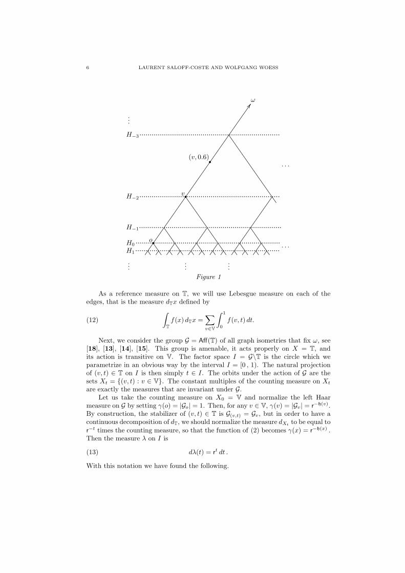
Let X = T be the 1-skeleton of the (r + 1)-regular tree and let V = V T be thevertex set of that tree. Choose a reference vertex o and a reference end (boundarypoint) ω of T regarded as a “mythical ancestor”. Draw T in horocycle layers withrespect to ω. Call H0 the horocycle of o. The other horocycles are labeled so thatHn contains the n-th descendant generation of o with respect to ω whereas H−n

contains the n-th ascendant generation of o with respect to ω. The tree T can beparametrized as T = V × [0 , 1) where, for any v ∈ V, {v} × [0 , 1) is the orientededge from v to its (uniquely defined) predecessor. We call this edge the 0-edge at vand we (arbitrarily) enumerate the r remaining edges as ei = {vi} × [0 , 1), wherevi, i = 1, . . . , r, are the successors of v. The discrete graph metric on V has anobvious “linear” extension to T. See Figure 1.

For v ∈ V, we set h(v) = n if v ∈ Hn. For x = (v, t) ∈ T = V × [0 , 1), we set

(11) n(x) = h(v) and h(x) = h(v) − t .

The horocycles in T are the sets Hs = {x = (v, t) : h(v, t) = s} , and if s = n − twith t ∈ [0 , 1) then Hs = {x = (v, t) : v ∈ Hn}.


......................................................................................................................................................................................................................................................................................................................................................................................................................................................................................................................................................................................................................................................................................................................

................

.....................................................................................................................................................................................................................................................................

..........................................................................................................................

..........................................................................................................................

.....................................................

.....................................................

.....................................................

.....................................................

..................

..................

..................

..................

..................

..................

..................

..................

................................................................................................................................................................................................................................................................................................................

.....................................................................................................................................................................................................................................................................

..................

..................

.....................................................

.....................................................

..................

..................

..........................................................................................................................

......

. . .

. . .

H−3

H−2

H−1

H0

H1

...

...

ω

o•

v•

(v, 0.6)•

Figure 1

As a reference measure on T, we will use Lebesgue measure on each of theedges, that is the measure dTx defined by

(12)

∫

T

f(x) dTx =∑

v∈V

∫ 1

0

f(v, t) dt.

Next, we consider the group G = Aff(T) of all graph isometries that fix ω, see[18], [13], [14], [15]. This group is amenable, it acts properly on X = T, andits action is transitive on V. The factor space I = G\T is the circle which weparametrize in an obvious way by the interval I = [0 , 1). The natural projectionof (v, t) ∈ T on I is then simply t ∈ I. The orbits under the action of G are thesets Xt = {(v, t) : v ∈ V}. The constant multiples of the counting measure on Xt

are exactly the measures that are invariant under G.Let us take the counting measure on X0 = V and normalize the left Haar

measure on G by setting γ(o) = |Go| = 1. Then, for any v ∈ V, γ(v) = |Gv| = r−h(v).

By construction, the stabilizer of (v, t) ∈ T is G(v,t) = Gv, but in order to have acontinuous decomposition of dT, we should normalize the measure dXt

to be equal tor−t times the counting measure, so that the function of (2) becomes γ(x) = r

−h(x) .Then the measure λ on I is

(13) dλ(t) = rt dt .

With this notation we have found the following.


Lemma 4.1. The Lebesgue measure dT on T has the continuous decomposition

∫

T

f(x) dTx =

∫ 1

0

[r−t∑

v∈V

f(v, t)

]dλ(t) ,

where the term in brackets is∫

Xtf(x)dXt

x .

4.B. Diffusions with constant coefficients. The transition operators thatwe want to study are those associated with the heat semigroups of conservative“constant coefficients” diffusions on T. To define these, we need some notation.

Let f be a function on T. For each vertex v, define fv to be the function onthe open interval (0 , 1) given by

fv(t) = f(v, t), t ∈ (0 , 1) ,

and set

fv(0) = limt→0

fv(t) and fv(1) = limt→1

fv(t) ,

whenever these limits exist. If fv is continuous on (0 , 1) and fv(0), fv(1) exist andare finite, we say that fv is continuous on [0 , 1].

Let dµ = m(·) dT be a measure with a positive density such that mv is continu-ous on [0 , 1] for each vertex v. Denote by H1

µ the space of all functions in L2(T, µ)whose distributional derivative on each interior edge v × (0 , 1) can be representedby a function f ′

v ∈ L2((0 , 1)

)and such that the function f ′ : (v, t) 7→ f ′

v(t) (which

is defined almost everywhere) is in L2(T, µ). Let H2µ be the space of those functions

f in H1µ such that f ′ ∈ H1

µ and define f ′′ accordingly. The spaces H1µ and H2

µ areequipped with the norms

‖f‖H1µ

=

(∫

T

(|f |2 + |f ′|2) dµ)1/2

and(14)

‖f‖H2µ

=

(∫

T

(|f |2 + |f ′|2 + |f ′′|2) dµ)1/2

,(15)

respectively, which turn them into Hilbert spaces. Let us note that any f in H1µ can

be represented by a function such that each fv is continuous on [0 , 1]. Similarly,any f ∈ H2

µ can be represented by a function such that fv and f ′v are continuous

on [0 , 1].We say that a function f is edgewise differentiable if fv admits a derivative

f ′v(t) on each open edge v × (0 , 1) . We say that f is edgewise C1 if it is edgewise

differentiable with continuous derivative f ′v on each open edge, and

limt→0

f ′v(t) = f ′

v(0) and limt→1

f ′v(t) = f ′

v(1)

both exist and are finite (i.e., f ′v is continuous on [0 , 1]). Note that such funcions

f need not be continuous at a given vertex v. If f is edgewise differentiable, we set

f ′(x) = f ′v(t) if x = (v, t) with t ∈ (0 , 1) ,

so that f ′ is well defined on T \ V. If f is edgewise C1, we set

f ′(x) = f ′v(t) if x = (v, t) with t ∈ (0 , 1) ,

f ′0(x) = f ′

v(0) if x = (v, 0) ,f ′

i(x) = f ′vi

(1) if x = (v, 0) ,


where {vi, 1 ≤ i ≤ r} is the set of all successors of v as introduced above. We willoften abuse notation and write f ′

i(v) for f ′i(v, 0).

We say that a function f is edgewise twice differentiable (resp. edgewise C2)if f is edgewise C1 and f ′ is edgewise differentiable (resp. edgewise C1). For sucha function, we set f ′′ = (f ′)′.

We are now ready to introduce our “constant coefficients” diffusions on T.

Definition 4.2. Let α, β be two real parameters with β > 0 . Let Dβ be thespace of all compactly supported, continuous edgewise C2 functions satisfying the“bifurcation” condition

(16) β

r∑

1

f ′i(x) = f ′

0(x) at each x = (v, 0) .

On Dβ, the “generator” L = Lα,β is defined by

(17) Lf(x) = f ′′(x) + αf ′(x) if x = (v, t) , t ∈ (0 , 1) .

Lemma 4.3. The operator L = Lα,β with domain Dβ is symmetric in L2(T, dµ) ,where the density dµ of the measure µ = µα,β is given by

(18) dµ(x) = m(x) dTx with m(x) = mα,β(x) = βn(x)e−αh(x).

Proof. On each open edge v × (0 , 1), integration by parts gives

∫ 1

0

f ′v(t)g

′v(t)β

n(v)e−αh(v)+αt dt = −∫ 1

0

f(v, t)(g′′v (t) + αg′v(t)

)βn(v)e−αh(v)+αt dt

+ fv(1)g′v(1)βn(v)e−αh(v)+α − fv(0)g′v(0)βn(v)e−αh(v) .

Now, at a given vertex v, the residual term coming from the r + 1 incident edges is

−βn(v)e−αh(v)fv(0)g′0(v) + βn(vi)e−αh(vi)+αfv(0)r∑

i=1

g′i(v)

= βn(v)e−αh(v)fv(0)

(−g′0(v) + β

r∑

i=1

g′i(v)

),

and it vanishes if g satisfies the boundary condition (17). �

In fact, (Lα,β, Dβ) is essentially self-adjoint in L2(T, dµα,β) . The proof requiressome serious efforts, see Bendikov, Saloff-Coste, Salvatori and Woess [2], and com-pare also with Bendikov and Saloff-Coste [1]. The domain of its unique self-adjointextension (still denoted L = Lα,β) is the set of all functions in H2

µ which are con-tinuous and satisfy (16). This self-adjoint operator L is the infinitesimal generatorof the Markov semigroup Hτ = eτL associated with the Dirichlet form

D(f) =

∫

T

|f ′(x)|2dµ(x)

with domain {f ∈ H1µ : f continuous} in L2(T, µ) . This Dirichlet form satisfies the

doubling property and Poincare inequality locally uniformly. By the very generalresults of Sturm [21], [22], [23], see also Saloff-Coste [12] and Eells and Fuglede[6], we have the following


Proposition 4.4. The semigroup Hτ admits a bounded continuous kernelhµ

τ (x, y) with respect to the reversible measure µ = µα,β . That is,

Hτf(x) =

∫

T

hµτ (x, y)f(y) dµ(y) .

Moreover, for each integer k ≥ 0,

(19)∣∣∂k

τ hµτ (x, y)

∣∣ ≤ Ck τ−k (min{1, τ})−1/2β−n(x)eαh(x)e−cd(x,y)2/τ

for all τ > 0 and x, y ∈ T. As hµτ (x, y) = hµ

τ (y, x), the factor β−n(x)eαh(x) can bereplaced by β−n(y)eαh(y) .

From this, it follows that Hτ can also be viewed as a semigroup acting onbounded continuous functions on T and that, in addition to the reversible measuredµ = m(·) dT, it admits also the measure dT as invariant measure. As a matter offact, for our computation, we will mostly use the kernel

hτ (x, y) = hµτ (x, y)m(y) ,

which is the kernel of Hτ with respect to the G-invariant measure dT. Indeed, thiskernel is invariant under the action of G, i.e., for each g ∈ G, hτ (gx, gy) = hτ (x, y) ,whereas this is not true for hµ

τ (x, y). Note that (19) and the subsequent remarkconcerning symmetry give

(20)∣∣∂k

τ hτ (x, y)∣∣ ≤ Ck (min{1, τ})−1/2e−c d(x,y)2/τ .

We will also need similar estimates for the space derivatives, up to the bifurcationpoints, namely, for every closed interval [a , b] ⊂ (0 , ∞) and all integers k,m ≥ 0,there is a constant Ca,b,k,m such that

(21) supτ∈[a , b]

sups∈(0 , 1)

∣∣∂kτ ∂

ms hτ

(x, (v, s)

)∣∣ ≤ Ca,b,k,m e−c d(x,v)2/b .

Please note the space derivatives are not continuous through the bifurcation points.These non-trivial estimates are derived in [2] in a more general context.

4.C. Reduction to the factor space and computations. Applying The-orem 2.1, we can compute the norm and spectral radius of Hτ on various spaces.Recall that I = G\T is the circle parametrised by the interval [0 , 1). For anys ∈ [0 , 1), set xs = (o, s) ∈ T. We will need to use the action of some elements ofG. Recall that oi, 1 ≤ i ≤ r are the “children” of o. For each 1 ≤ i ≤ r, let gi be afixed element of G such that gioi = o. Since all elements of G fix ω, the image of ounder gi must be the unique predecessor of o.

Spectral radii on Lp(T, dµ). Let µ = µα,β be the measure defined in Lemma4.3. In the case of Lp(T, µ), Theorem 2.1 does not directly apply since µ is notinvariant under G. Hence, we must instead use Remark 2.2 following Theorem 2.1.Accordingly, for a fixed p ∈ (1,∞), we consider the operator Aτ , τ > 0, acting onLp(I, dλ) with kernel

(22)

aτ (s, t) =

∫

Xt

(γ(y)m(xs)

γ(xs)m(y)

)1/p

hτ (xs, y) dXty

= r−t∑

v∈V

(r e−α)−(h(v)−t+s)/pβ−n(v)/p hτ

(xs, (v, t)

).

By (20) and (21), this is a bounded, smooth kernel on [0 , 1). It follows that Aτ

is a compact operator on Lr(I, dλ) for any 1 < r < ∞ (see, e.g., Schaefer [17, p.


283]) and, by (7), the family (Aτ )τ>0 forms a semigroup of bounded operators. Itfollows from the Gaussian bound (20) that this semigroup is C0. As any Lr(I, dλ)-eigenfunction for Aτ must be bounded, the spectrum of Aτ is independent of r.Let ρτ = ρ(Aτ ) be the spectral radius of Aτ on Lr(I, dλ). Since Aτ1

Aτ2= Aτ1+τ2

,there are ω ≥ 0 and a positive function u on I such that

(23) ρτ = e−ωτ and Aτu = e−ωτu

We are going to compute ω as the smallest real eigenvalue of a simple eigenvalueproblem, see (25) below.

As a function of s ∈ [0 , 1), aτ (s, t) is smooth on [0 , 1). We now study itsone-sided limits at the endpoints. Recall that the interval parametrizes the circle.We shall see that aτ (s, t) and its derivatives have jumps at the endpoints of theinterval when the latter are identified on the circle. The following two limits exist:

(24)aτ (1, t) = lim

s→1aτ (s, t) and ∂B

s aτ (1, t) = lims→1

∂Bs aτ (s, t) ,

where B = (r e−α)−1/p and ∂Bs = Bs∂sB

−s .

Lemma 4.5. (a) We have

aτ (1, t) = β1/p aτ (0, t) and β r ∂Bs aτ (1, t) = β1/p ∂B

s aτ (0, t) .

(b) For s ∈ (0 , 1),

∂τaτ (s, t) =(∂B

s

)2aτ (s, t) + α ∂B

s aτ (s, t) .

Proof. Regarding the first identity of (a), recall that g1o is the unique prede-cessor of o. We compute

rtaτ (1, t) =

∑

v∈V

Bh(v)−t+1 β−n(v)/p hτ

((g1o), (v, t)

)

=∑

v∈V

Bh(v)−t+1 β−n(v)/p hτ

(o, (g−1

1 v, t))

=∑

v∈V

Bh(g−1

1v)−t β−(n(g−1

1v)−1)/p hτ

(o, (g−1

1 v, t))

=∑

v∈V

Bh(v)−t β−(n(v)−1)/p hτ

(o, (v, t)

)= β1/p

rt aτ (0, t)

For the second identity of (a), set hyτ (x) = hτ (x, y). Then

rt ∂B

s aτ (s, t) =∑

v∈V

Bh(v)−t+s β−n(v)/p ∂sh(v,t)τ (xs).

Observe that for each i ∈ {1, . . . , r}, we have

lims→1

∂shyτ

((o, s)

)= lim

s→1∂sh

yτ

((gioi, s)

)

= lims→1

∂shg−1

iy

τ

((oi, s)

)=(h

g−1

iy

τ

)′i(o),


and compute

rt ∂B

s aτ (1, t) =∑

v∈V

Bh(v)−t+1 β−n(v)/p(h

(g−1

iv,t)

τ

)′i(o)

=∑

v∈V

Bh(g−1

i v)−t β−(n(g−1

i v)−1)/p(h

(g−1

iv,t)

τ

)′i(o)

= β1/p∑

v∈V

Bh(v)−t β−n(v)/p(h(v,t)

τ

)′i(o) .

Now the identity follows after recalling that the function hyτ must satisfy (16), that

is,

βr∑

1

(hy

τ

)′i(v) =

(hy

τ

)′0(v).

Finally, for s ∈ (0 , 1), aτ (s, t) is smooth, and by (17),

∂τhτ

((o, s), y

)= ∂2

shτ

((o, s), y

)+ α∂shτ

((o, s), y

).

The identity (b) follows. �

(23) and Lemma 4.5 lead to the eigenvalue problem

(25)

(∂B

s

)2u(s) + α∂B

s u(s) = −ω u(s) on (0 , 1)

u(1) = β1/p u(0)

r β ∂Bs u(1) = β1/p ∂B

s u(0)

where the values of u and ∂Bs u at 0 and 1 must be understood as limits as s tends

to either 0 or 1. Setting v(s) = B−su(s), we find the following.

Corollary 4.6. The spectral radius of Aτ on Lp(I, λ) is ρτ = e−ωτ , where ωis the smallest real solution of

(26)

v′′(s) + αv′(s) = −ω v(s) on (0 , 1)

v(1) = b1/p v(0) ,

v′(1) = (r β)−1 a1/p v′(0) ,

where b = b(α, β) = B−p β = r β e−α > 0 .

We can now solve (4.6). If 4ω 6= α2 and ω > 0, the general real solution ofv′′ + αv′ + ω v = 0 is

v(s) = c1 e(−α+z)s/2 + c2 e

(−α−z)s/2

with

z =

{√α2 − 4ω , if α2 > 4ω

i√

4ω − α2 , if α2 < 4ω .

We are lead to the linear system{

c1(e(−α+z)/2 − b1/p

)+ c2

(e(−α−z)/2 − b1/p

)= 0

c1(−α+ z)(e(−α+z)/2 − (r β)−1 b1/p

)+ c2(−α− z)

(e(−α−z)/2 − (r β)−1 b1/p

)= 0 .

This linear system has a non-trivial solution (c1, c2) if and only if its determinantis 0, which leads to the equation

(27) α(β r − 1)sinh(z/2)

z= (β r + 1) cosh(z/2)− eα/2

((r β e−α)b−1/p + b1/p

).


If we substitute z = i ζ then (27) becomes

(28) α(β r − 1)sin(ζ/2)

ζ= (β r + 1) cos(ζ/2) − eα/2

((r β e−α)b−1/p + b1/p

).

The last term can of course be simplified to((r β e−α)b−1/p + b1/p

)= (b1/p + b1−1/p) ,

but we shall need it in the above form later on. We can now summarize thecomputation of ω. In the following theorem, we first consider three special cases.

Theorem 4.7. The spectral gap ω = ωp(α, β) of the operator Lα,β acting onthe space Lp(T, dµα,β) is given as follows.

(I) No continuous drift: α = 0 . Then

ω =

[arccos

((rβ)1/p + (rβ)1−1/p

1 + rβ

)]2.

In particular, if α = 0 and β = 1/r then ω = 0.

(II) No discrete drift: β = 1/r . Then

ω = α2p−1(1 − p−1

).

(III) No total drift: b(α, β) = r β e−α = 1 . Then ω = 0 , there is no spectral gap.

(IV) The general case: α 6= 0 , βr 6= 1 , r β e−α 6= 1 .

(IV.i) If α(β r − 1) < 2(β r + 1 − eα/2

(b(α, β)1/p + b(α, β)1−1/p

))then

ω =1

4(α2 + ζ2

0 ) ,

where ζ0 is the smallest positive solution (in ζ) of (28).

(IV.ii) If α(β r − 1) ≥ 2(β r + 1 − eα/2

(a(α, β)1/p + a(α, β)1−1/p

))then

ω =1

4(α2 − z2

0) ,

where z0 is the unique positive real solution of (27).

Proof. (I) When α = 0, equation (28) becomes

cos√ω =

(r β)1/p + (r β)1−1/p

1 + r β.

Note that the right hand side is in (0 , 1]. In the special case α = 0 , β = 1/r, wehave no spectral gap (ω = 0 is solution) and (26) with ω = 0 admits the constantfunction v ≡ 1 as a solution.

(II) When β = 1/r, equation (27) gives

cosh(z/2) = cosh(α(1/2 − 1/p)

),

leading to the proposed smallest positive solution for ω.

(III) If b(α, β) = 1 , it is easy to check directly that (26) admits ω = 0, v ≡ 1 has asolution.

(IV.i) In this case, (27) has no real solution, so that we need the smallest positivereal solution ζ0 = ζ0(r, α, β, p) of (28).


(IV.ii) In the second case, (27) has a unique real positive solution z0 = z(r, α, β, p) ,and ω = (α2 − z2

0)/4 .

In particular, when α(β r − 1) = 2(β r + 1 − eα/2

(b(α, β)1/p + b(α, β)1−1/p

))

then the characteristic equation of the differential equation v′′ + αv′ + ωv = 0 hasa double root, and the general form of the solution is (c1 + c2 s)e

−αs/2 . Thus, oneeasily checks that ω = α2/4 is indeed a solution. �

We remark that in the case p = 2, our analysis shows that

ω ≥ α2/4 if and only ifα(1 +

√r β)√

r β − 1≤ 1 .

We also remark that Cattaneo [4] considers an analog of the operator L0,β on generalnetworks and relates the L2-spectrum of that Laplacian with the ℓ2-spectrum of thetransition operator on the vertex set of the network. In particular, on can combineher results with the well-known formula for the spectral radius of simple randomwalk on the tree to obtain ω = ω2(0 , 1), corresponding to case (I) of Theorem 4.7with β = 1 and p = 2.

Spectral radii with respect to other measures on T. By (20), the semigroupHτ = e−tL not only acts on Lp(T, dµα,β), but also on Lp(T, dµκ,η), with the measureµκ,η defined as in (18) for any κ ∈ R and η > 0 in the place of α and β. In particular,Lp(T, dT) corresponds to κ = 0 , η = 1.

Accordingly, for a fixed p ∈ (1,∞), we consider the operator Aτ , τ > 0, actingon Lp(I, dλ) with kernel

aτ (s, t) =

∫

Xt

(γ(y)mκ,η(xs)

γ(xs)mκ,η(y)

)1/p

hτ (xs, y) dXty

= r−t∑

v∈V

(r e−κ)−(h(v)−t+s)/p η−n(v) hτ

(xs, (v, t)

).

An analysis similar to that of the special case of Lp(T, dµα,β) shows that thespectral radius of Aτ is e−ωτ where ω is the smallest real solution of the sameeigenvalue problem as in (26), but with different constant

(29) b = b(κ, η) = r η e−κ > 0 .

In this situation, since Lα,β is in general not negative semi-definite on Lp(T, dµκ,η),we can no more speak of the “spectral gap”, since ω may also become negative. Weget the following results (with arcosh = cosh−1).

Theorem 4.8. With b = b(κ, η) as in (29), the top of the spectrum −ω =−ωp(α, β;κ, η) of the operator Lα,β acting on the space Lp(T, dµκ,η) is given asfollows.

(I) No continuous drift: α = 0 . Then

ω =

[arccos

(b1/p + r β b−1/p

1 + r β

)]2, if (b1/p − r η)(b1/p − 1) < 0,

[arcosh

(b1/p + r β b−1/p

1 + r β

)]2, if (b1/p − r η)(b1/p − 1) ≥ 0 .


(II) No discrete drift: β = 1/r . Then

ω = αlog b

p−∣∣∣∣log b

p

∣∣∣∣2

.

(III) The case r η e−κ = 1 : Here, b = 1 and ω = 0.

(IV) The general case: α 6= 0 , r β 6= 1 , r η e−κ 6= 1 .

(IV.i) If α(r β − 1) < 2((r β + 1) − eα/2

((r β e−α) b−1/p + b1/p

))then

ω =1

4(α2 + ζ2

0 ) ,

where ζ0 is the smallest positive solution (in ζ) of (28).

(IV.ii) If α(β r − 1) ≥ 2((r β + 1) − eα/2

((r β e−α) b−1/p + b1/p

))then

ω =1

4(α2 − z2

0) ,

where z0 is the unique positive real solution of (27).

5. Convolution on locally compact connected groups

5.A. Unravelling Theorem 2.1. This section relates Theorem 2.1 to ques-tions of classic harmonic analysis. To preserve natural notation, we will have tochange our own notation a bit. Let X = G be a locally compact group equippedwith a fixed left Haar measure dG . Denote by ∆G the modular function on G.

While primarily we have in mind the case when the group is connected, weshall see on several occasions that this is not necessarily required.

Let us assume that the kernel k(x, y) ≥ 0 is a continuous function of (x, y),that

∫X k(x, y)dGy = 1, and that the operator

(30) Kf(x) =

∫

X

k(x, y)f(y) dGy

is invariant under the left action of G. In this case, if we set

(31) φ(y) = φG(y) = k(e, y−1) = k(y, e), dΦ = φdG ,

we have

(32)

Kf(x) = f ∗ Φ(x) =

∫

G

φ(y−1x) f(y) dGy

=

∫

G

f(xy−1)∆G(y)−1 φ(y) dG y

that is, K = RΦ is the operator of right convolution by the probability measure Φ(or equivalently, by its density, the function φ) on G. Obviously, we could as wellhave started with φ on G and set k(x, y) = φ(y−1x). We are interested in computingthe norm σp(K) ∈ (0 , 1] and spectral radius ρp(K) ∈ (0 , 1] of K = RΦ acting onLp(G, dG), 1 < p <∞ (right convolution operator, but left Haar measure !).

By Theorem 2.1, these numbers equal one if and only if G is both amenable andunimodular. Our goal is to get a better understanding of what happens when G isnon-unimodular or non-amenable or both, under the additional assumption that Gis connected. It will be useful to proceed in several steps.


Step 1: reduction to the semisimple case with finite center. We startwith the following simple application of Theorem 2.1, valid also without assumingconnectedness. For connected groups it provides the reduction addressed above.

Proposition 5.1. Let G be a locally compact group and let K, k, φ be as above.Let Q be a closed normal amenable subgroup and L = Q\G. Then, for any 1 ≤ p ≤∞,

σp(K) = σp(KL) and ρp(K) = ρp(KL) ,

where KL is the left invariant operator acting on Lp(L) associated with the kernel

kL(u, v) =

(∆G(x−1

v xu)

∆L(v−1u)

)1/p∆G(xv)

∆L(v)

∫

Q

∆G(y)−1/p k(xu, yxv) dQy.

Here xu ∈ G denotes any representative of u ∈ L.

Proof. By Bourbaki [3, chap. VII, §2], we have ∆G(x) = ∆Q(x) for all x ∈ Q.Moreover, there exists a continuous decomposition of dGx under the left action ofQ such that the mesure dλ on the quotient L = I = Q\G is the left Haar measureon L. Note that in [3, chap VII, §2], the quotient by Q (called G′ in [3]) is the rightquotient so that some translation is needed to obtain the desired decomposition.Namely, for any f ∈ C00(X) we have

∫

G

f(g) dGg =

∫

L

{∆G(xu)

∆L(u)

∫

Q

f(yxu) dQy

}dLu .

In this decomposition, the invariant measure dXuξ on the orbit

Xu = {ξ = yxu : y ∈ Q}equals

dXuξ =

∆G(xu)

∆L(u)dQy .

Note that here {e} = Gx ⊂ Q ⊂ G is the stabilizer of x ∈ G under the left action ofQ. Hence, formula (1) shows that, for each u ∈ L, x ∈ Xu, we have

γ(x) = |{e}|Gx=

∆L(u)

∆G(x).

With these remarks, the proposition is immediately deduced from Theorem 2.1. �

Remark 5.2. By [3, chap. VII, §2], if for x ∈ G we set φx : Q → Q, y 7→ x−1yxthen ∫

Q

f(φ−1

xu(y))dQy =

∆G(xu)

∆L(u)

∫f(y) dQy .

It follows that we can write

kL(u, v) =

(∆G(x−1

v xu)

∆L(v−1u)

)1/p ∫

Q

∆G(y)−1/p k(xu, xvy) dQy

=

(∆G(x−1

v xu)

∆L(v−1u)

)1/p ∫

Q

∆G(y)−1/p k(x−1v xu, y) dQy .

This shows that the operator KL is a (right) convolution operator on L, i.e.,

kL(u, v) = φL(v−1u)


depends only on v−1u. The correspondence between φ and φL is given by

φL(u) = ∆L(u)−1/p

∫

Q

∆G(y−1xu)1/p φ(y−1xu) dQy .

For p, q ∈ (1,∞) such that 1/p+ 1/q = 1, denote by φp,L, φq,L the correspondingfunctions on L. Then, we have

(φ)p,L(u) = ∆L(u)−1/p

∫

Q

∆G(xu−1y)−1/p φ(xu−1y) dQy

= ∆L(u)1/q

∫

Q

∆G(yxu−1 )−1/p∆G(xu−1)φ(yxu−1 ) dQy

= ∆L(u−1)−1/q

∫

Q

∆G(y−1xu−1 )1/q φ(y−1xu−1) dQy

= φq,L(u−1) = (φq,L ) (u) .

This is consistent with the fact that if K is the operator of right convolution by afunction φ on a group G, its formal adjoint K∗ is right convolution by φ and forp, q ∈ [1,∞] with 1/p+ 1/q = 1, σq(K) = σp(K

∗).

Step 2: unimodular groups of type PK, where P is amenable and Kcompact. Let L be a locally compact unimodular group such that there are closedsubgroups P ,K with P amenable and K compact such that L = PK . Let

kL(u, v) = φL(v−1u)

be a left invariant kernel under the action of L. In particular, kL is left invariantunder the action of the closed amenable subgroup P . Thus we can apply Theorem2.1. In general, P is not normal in L and the quotient space

I = P\L = [K ∩ P ]\Kis compact. Let dλ be the uniqueK invariant measure on I such that the normalizedHaar measures on K and K ∩ P satisfy dKv = dK∩Pxdλ(s) . Classical results showthat there is a continuous decomposition of the Haar measure on L as

dLu = dPxdλ(s) , s ∈ I, u = s mod Pwith γ(x) = ∆P (x)−1. Again, γ(x) = |{e}|Gx

where {e} = Gx ⊂ P ⊂ L is viewedas the stabilizer of x ∈ L under the left action of P .

For any u = xv ∈ L with x ∈ P , v ∈ K, we set

(33) ∆LP(u) = ∆P(x).

This makes sense because if u = xv ∈ L, x ∈ P , v ∈ K and u = x′v′ ∈ L withx′ ∈ P , v′ ∈ K then v′v−1 ∈ P ∩K and thus ∆P(v′v−1) = 1 (P ∩K is a compact).Hence ∆P(x′) = ∆P (x). We insist in using this somewhat cumbersome notationinstead of a lighter alternative such as ∆P(u), because in general, for u, v ∈ L,

∆LP(uv) 6= ∆L

P(u)∆LP(v).

In this context, Theorem 2.1 leads to the study of the operator with kernel

kI(s, t) =

∫

P

∆P(x)−1/pkL(s, xt) dPx .

acting on Lp(I, dλ), 1 < p < ∞. However, one can lift this operator from thequotient space I = [K ∩ P ]\K to K in an obvious way without changing its normor spectral radius. This gives the following.


Proposition 5.3. Let L be a unimodular locally compact group such thatL = PK for two closed subgroups P ,K with P amenable and K compact. LetkL(u, v) = φL(v−1u) be a left invariant kernel on L as above. Fix p, q ∈ [1,∞] with1/p+ 1/q = 1. Then

σp(KL) = σp(KK) and ρp(HL) = ρp(KK) ,

where KK is the operator on Lp(K) with kernel

kK(s, t) =

∫

P

∆P(x)−1/p kL(s, xt) dPx .

In particular, we have the following results:

(a)

σp(KL) ≤{∫

K

[∫

K

(∫

P

∆P(x)−1/p kL(s, xt) dPx

)q

dKt

]p/q

dKs

}1/p

.

(b) Assume that kL(e, vs) = kL(e, sv) for all s ∈ K , v ∈ L. Then

σp(KL) = ρp(KL) =

∫

L

∆LP(v)−1/p kL(e, v) dLv .

(c) Assume that kL(e, vs) = kL(e, v) for all s ∈ K, v ∈ L. Then

σp(KL) =

[∫

K

(∫

P

∆P(x)−1/pkL(s, x)dPx

)p

dKs

]1/p

and, assuming σp(KL) <∞ ,

ρp(KL) =

∫

L

∆LP (v)−1/q kL(v, e) dLv .

(d) Assume that kL(e, sv) = kL(e, v) for all s ∈ K, v ∈ L. Then

σp(KL) =

[∫

K

(∫

P

∆P(x)−1/p kL(e, xs) dPx

)q

dKs

]1/q

and, assuming σp(KL) <∞ ,

ρp(KL) =

∫

L


Proof. To prove this proposition, we apply Theorem 2.1. Part (a) follows froma standard estimation of σp(KK).

For (b), observe that kK(s, t) depends only on t−1s. Hence KK is a convolutionoperator with non-negative kernel on K and its norm equals its spectral radius,which equals

∫KkK(e, s) dKs.


We have KKf(s) =(∫

Kf dK

)kK(s, e). The formula for σp(KL) follows. More-

over,

(34)

ρp(KL) =

∫

K

∫

P

∆P(x)−1/p kL(s, x) dPxdKs

=

∫

K

∫

P

∆P(x−1)−1/q ∆P (x−1) kL(x−1s, e) dPxdKs

=

∫

K

∫

P

∆P(x)−1/q kL(xs, e) dPxdKs

=

∫

L

∆LP(v)−1/q kL(v, e) dLv ,

as stated.In (d) we have KKf(s) =

∫KkK(e, t)f(t) dKt , and the desired results follow

since

ρp(KL) =

∫

K

∫

P

∆P(x)−1/p kL(e, xs) dPxdKs =

∫

L


Note that (c) and (d) are dual to each other by passing to the adjoint operator (i.e.,changing kL(u, v) to kL(v, u)). �

The following statement is a simple corollary of Proposition 5.3 together withthe characterization of amenability in terms of convolution operator norms (see [5,Prop. 4.2] and [15]).

Proposition 5.4. Let L be a locally compact unimodular group of type PKwith P ,K two closed subgroups, P amenable, K compact. Then L is non-amenableif and only if P is non-unimodular.

The results of this section apply to real connected semisimple Lie group withfinite center and to the group of K-points of a connected (in the Zariski topology)linear algebraic semisimple group defined over the local field K. In both cases thereare Iwasawa decompositions that yield L = PK with P ,K closed subgroups, Pamenable, K compact. In the general case of algebraic groups, the intersection ofP and K may not be reduced to {e}. Other interesting cases arise as subgroups ofthe automorphism group of a free group, see Nebbia [10]. We next give details inthe case of connected Lie groups with finite center.

The case of semisimple Lie groups with finite center

One of the most important examples of groups of type PK with P amenable and Kcompact are non-compact connected semisimple Lie group with finite center. LetL be such a group. Then L is unimodular and admits an Iwasawa decompositionL = NAK with K compact and P = NA amenable, K ∩ P = {e}.

Although P is not normal in L, we can identify L with PK and P\L with Kas manifolds, and we have the decomposition

dLu = dPxdKs ,

if u = xs, x ∈ P , s ∈ K.As usual, we denote by ∆P the modular function of P . This is a N -bi-invariant

function on P , and

(35) ∆P(x) = e−2ρL(log a) , if x = na (n ∈ N , a ∈ A) ,


where ρL denotes the half sum of the positive roots weighted by their multiplicities,see, e.g., Helgason [8, p 181]) To relate these results with classic theory, we introducethe function ψτ , τ ∈ R, defined by

(36) ψτ (x) =

∫

K

∆LP(sx)−(τ+1)/2ds .

Denote by A the Lie algebra of A. Recall that for each complex valued linear formλ on A, the elementary spherical function ϕλ is defined by

ϕλ(x) =

∫

K

exp(iλ(log a(sx)

)+ ρL

(log a(sx)

))ds ,

where a(x) denotes the A-component of x ∈ L in its NAK decomposition, ρL isthe half sum of the positive roots, and log a is the element of A whose image by theexponential map is a. See [8, Theorem 4.3]. From (35), it follows that

(37) ψτ = ϕ−i τρ .

By [8, Lemma 4.4], this implies

(38) ψτ (x−1) = ψ−τ (x).

With this notation, Proposition 5.3 leads to the following.

Theorem 5.5. Let L be a non-compact connected semisimple Lie group withfinite center and Iwasawa decomposition L = PK, P = NA. Let φ be a non-negative function on L and let K denote the operator of right convolution by φ asin (32). Fix p, q ∈ [1,∞] with 1/p+ 1/q = 1.

(i) Assume that φ(us) = φ(su) for all s ∈ K , u ∈ L. Then

σp(K) = ρp(K) =

∫

L

ψ1−2/p(v)φ(v) dLv .

(ii) Assume that either φ(u) = φ(su) for for all s ∈ K , u ∈ L and∫

K

(∫

P

∆P(x)−1/p φ(x−1s) dPx

)p

dKs <∞ ,

or that φ(u) = φ(us) for all s ∈ K , u ∈ L and∫

K

(∫

P

∆P(x)−1/pφ(sx−1) dPx

)q

dKs <∞ .

Then we have

ρp(K) =

∫

L


Proof. Regarding (i), Proposition 5.3(b) gives

σp(K) = ρp(K) =

∫

L

∆LP (v)−1/p φ(v−1) dLv .

Using the fact that φ is invariant under K-inner automorphisms and ∆LP right

K-invariant, we find that, for any s ∈ K,∫

L

∆LP(v)−1/p φ(v−1) dLv =

∫

L

∆LP(sv)−1/p φ(v−1) dLv .


Hence, by (37) and (38),

σp(K) =

∫

L

∫

K

∆LP(sv)−1/p dKs φ(v−1) dLv

=

∫

L

ψ−(1−2/p)(v)φ(v−1) dLv

=

∫

L


Regarding (ii), if φ(u) = φ(su) for for all s ∈ K , u ∈ L, then kL(u, v) = φ(v−1u)satisfies kL(e, vs) = kL(e, v) for all v ∈ L, s ∈ K. Hence (34) applies and gives

ρp(K) =

∫

K

∫

P

∆P(x)−1/p kL(s, x) dPxdKs

=

∫

K

∫

P

∫

K

∆LP(xt)−1/p kL(s, xt) dPxdKt dKs

=

∫

K

∫

L

∆LP(v)−1/p kL(s, v) dLv dKs

=

∫

K

∫

L

∆LP(v)−1/p kL(e, s−1v) dLv dKs

=

∫

K

∫

L

∆LP(sv)−1/p kL(e, v) dLv dKs

=

∫

L

ψ1−2/p(v)φ(v) dLv dKs .

The last case where φ(u) = φ(us) for all s ∈ K , u ∈ L is analogous. �

Step 3: General locally compact connected groups. Let us now explain howone can apply Steps 1 and 2 in the case of connected locally compact groups. Anyconnected locally compact group G contains a compact normal subgroup M suchthat M\G is a Lie group. Next, we consider the radical R of M\G. By definition,R is the largest connected closed normal solvable subgroup of M\G. See, e.g.,Paterson [11, Prop. 3.7] and Varadarajan [24]. Set S = R\[M\G]. Then Sis a connected semisimple Lie group and there exists a central discrete subgroupZ ∼= Z

d ⊂ S (for some integer d ∈ {0, 1, . . .}) such that L = Z\S is a connectedsemisimple Lie group with finite center. By this construction we have a surjectivegroup homomorphism from G to L. The kernel Q of this homomorphism is a closednormal subgroup, and it is amenable. Indeed, M is a closed normal subgroup of Qand M\Q, viewed as a subgroup of M\G, contains R as a closed normal subgroup.Finally, R\[M\Q] = Z. Now, Z is abelian, R is solvable and M is compact. Hencethey are all amenable, and so is Q by [11, Prop 1.13]. Of course, we have

(39) L = Q\G .

Let K be a left invariant transition operator on G as in (30). Let Q and L beas above in (39). Proposition 5.1 yields a left invariant transition kernel kL on thesemisimple Lie group L. Now, it is well known that L is compact if and only if G isamenable; see e.g. [11, Th. 3.8]. Assume that L is compact. Then we can compute


the norm and spectral radius of K on Lp(G) as

σp(K) = ρp(K) =

∫

L

kL(u, v) dLv

=

∫

L

∫

Q

∆G(x−1v xu)1/p ∆G(y)−1/p∆G(xv) k(xu, yxv) dQy dLv

=

∫

G

(∆G(xu)

∆G(g)

)1/p

k(xu, g) dg =

∫

G

∆G(g)−1/pφ(g−1) dg.

This yields

σp(K) = ρp(K) =

∫

G

∆G(g)−1/pφ(g−1) dg =

∫

G

∆G(g)−1+1/p dΦ(g) .

Of course, this conclusion is well known and true in complete generality as soon asG is amenable. In fact, this formula is at the heart of the proof of Theorem 2.1 in[15].

The more interesting case is when L is non-compact. In order to unravel ourcomputation, we need to introduce the following notation. By construction, L issemisimple with finite center and we let

(40) L = PK , P = NAbe an Iwasawa decomposition as in Step 2 above.

Define ∆GP on G by setting

∆GP (g) = ∆L

P ◦ πG,L(g) ,

where ∆LP is defined by (33) and πG,L denotes the canonical projection from G onto

L = Q\G.Similarly, define

ψτ (g) = ψτ (πG,L(g))

with ψτ as in (36).With these definitions, Proposition 5.3 gives the following result.

Theorem 5.6. Let G be a locally compact, connected group and K be a leftinvariant transition operator on G as in (30). Let φ be defined by (31). Let Q, Lbe as in (39) and K be as (40).

(i) Assume that kL(e, vs) = kL(e, sv) for all s ∈ K, v ∈ L. Then

σp(K) = ρp(K) =

∫

G

[∆G

P(g)∆G(g)]−1/p

φ(g−1) dGg

=

∫

G

ψ1−2/p(g)[∆G(g)

]−1/pφ(g−1) dGg.

(ii) Assume that K is bounded on Lp(G, dGg) and kL(e, vs) = kL(e, v) for alls ∈ K, v ∈ L. Then

ρp(K) =

∫

G

[∆G

P (g)∆G(g)]−1/q

φ(g) dGg

=

∫

G

ψ1−2/p(g)[∆G(g)

]−1/qφ(g) dGg.


(iii) Assume that K is bounded on Lp(G, dGg) and that kL(e, sv) = kL(e, v) forall s ∈ K, v ∈ L. Then

ρp(K) =

∫

G

[∆G

P(g)∆G(g)]−1/p

φ(g−1) dGg

=

∫

G

ψ1−2/p(g)[∆G(g)

]−1/pφ(g−1) dGg.

Proof. We prove (i). Statements (ii) and (iii) follows by similar arguments. ByPropositions 5.1 and 5.3, we have σp(K) = ρp(K), and (letting xv be, as usual, arepresentative of v ∈ L in G)

σp(K) =

∫

L

∆LP(v)−1/p kL(e, v) dLv

=

∫

L

∫

Q

∆GP

(xv)−1/p ∆G(yxv)−1/p ∆G(xv) k(e, yxv) dQy dLv

=

∫

L

∫

Q

[∆G

P(yxv)∆G(yxv)]−1/p

∆G(xv) k(e, yxv) dQy dLv

=

∫

G

[∆G

P(g)∆G(g)

]−1/pk(e, g) dGg

=

∫

G

[∆G

P(g)∆G(g)]−1/pφ(g−1) dG g

as desired. The formula using ψ1−2/p follows by a similar computation using The-orem 5.5. �

5.B. An example: convolutions on Aff+(R2). In this section we mostlyfollow the notation of Lang [9] (except for what [9] calls the modular function ∆ is∆−1 for us). The group G = Aff+(R2) is the group of orientation preserving affinetransformations of the plane, that is, Aff+(R2) = GL+

2 (R) ⋉ R2 where GL+

2 (R) isthe group of all invertible two by two matrices with real coefficients and positivedeterminant. The action of GL+

2 (R) on R2 is the natural action. Thus the product

is given by

(m, ξ)(m′, ξ′) = (mm′, ξ + mξ′) .

Any element m of GL+2 (R) decomposes as m = t · l where t > 0 and t2 is the

determinant of m, and l is in SL2(R). The group GL+2 (R) is unimodular with

Haar measure dm = t−1 dt dl where dl is a Haar measure on SL2(R). The groupG = Aff+(R2) is non-unimodular with left Haar measure

dGg = det(m)−1 dm dξ if g = (m, ξ) ,

and modular function

∆G(g) = det(m)−1 .

Observe that we can write

G = Aff+(R2) = SL2(R) ⋉[R ⋉ R

2]

where the action of R on R2 is by dilation. When applying the result of Section

5.A to this example, we can take Q = R ⋉ R2 and L = SL2(R).


Any element l of L = SL2(R) has a unique decomposition of the form

l = lx,y,s = nx ay ks , x ∈ R , y > 0 , s ∈ [0, 2π) ,

corresponding to the NAK = PK Iwasawa decomposition of SL2(R) where

nx =

(1 x0 1

), ay =

( √y 0

0 1/√y

), ks =

(cos s sin s− sin s cos s

).

In these coordinates, the Haar measure on L = SL2(R) is

dLl = y−2 dx dy ds .

and we have

∆LP (l) = y−1 .

The pair (x, y) corresponds to a point in the hyperbolic upper half plane L/K. Inparticular, the functions on L which satisfy φL(kl) = φL(lk) for all k ∈ K , l ∈ L arethose of the form

(41) φL(lx,y,s) = f(z, s) with z = [x2 + (y − 1)2]/y

whereas the functions on L which satisfy φL(l) = φL(lk) are those of the form

(42) φL(lx,y,s) = f(x, y).

Let φ(g) be a non-negative function on G = Aff+(R2) and consider the oper-ator K on Lp(G) with kernel k(g, h) = φ(h−1g). Then the corresponding kernelkL(u, v) = φL(v−1u) on L = SL2(R) is given by

φL(l) =

∫

Q

t2/p φ((t, ξ)−1(l, 0)

) dt dξt3

=

∫

Q

t2/pφ((t−1 · l, t−1 · ξ)

) dt dξt3

.

Here, the t in (t, ξ) stands for dilation by the factor t, that is, for t times the identitymatrix.

In view of (41) and (42), we are going to look at two classes of functions onG = Aff+(R2) in the coordinate system

g = gt,x,y,s,ξ = (t · nx ay ks, ξ) ,

namely, the functions given by

(43) φ(gt,x,y,s,ξ) = f(t, z, s, ξ) with z = [x2 + (y − 1)2]/y

and those given by

(44) φ(gt,x,y,s,ξ) = f(t, x, y, ξ) .

Proposition 5.7. On G = Aff+(R2), consider an operator K as in (30) withkernel k(x, y) = φ(y−1x).

(i) If φ is as in (43) then

σp(K) = ρp(K) =

∫

R2

∫

[0,2π)

∫

R+

∫

R

∫

R+

f(t, [x2 + (y2 − 1)]/y, s, ξ)dt dx dy ds dξ

t1+2/py2+1/p.

(ii) If K is bounded on Lp(G, dGg) and φ is as in (44) then

ρp(K) =

∫

R2

∫

R+

∫

R

∫

R+

f(t, x, y, ξ)dt dx dy dξ

t1+2/py2+1/p.


References

[1] Bendikov, A. and Saloff-Coste, L.: Smoothness and heat kernels on metric graphs. In Preprint(2008).

[2] Bendikov, A., Saloff-Coste, L., Salvatori, M. and Woess, W.: Brownian motion and harmonic

functions on treebolic spaces. In preparation.[3] Bourbaki, N.: Integration. Chap. 7-8. Hermann, 1963.[4] Cattaneo, C.: The spectrum of the continuous Laplacian on a graph. Monatsh. Math. 124

(1997), 215–235.[5] Chatterji, I., Pittet, C. and Saloff-Coste, L.: Connected groups and property RD. Duke Math.

J. 137 (2007), 511–536.[6] Eells, J. and Fuglede, B.: Harmonic Maps between Riemannian Polyhedra. 2001, Cambdridge

Tracts in Mathematics 142, Cambridge University Press.[7] Hardy G.H., Littlewood J.E. and Polya G.: Inequalities. Cambridge Univesrity Press, 1952.[8] Helgason, S.: Groups and Geometric Analysis. Academic Press, 1984.[9] Lang, S.: SL2(R). Springer, 1975.

[10] Nebbia, C.: Amenability and Kunze-Stein property for groups acting on a tree. Pacific J.Math. 135 (1988) 371–380.

[11] Paterson, A.: Amenability. Math. Surv. Monographs, Vol. 29. American Mathematical Soci-ety, 1988.

[12] Saloff-Coste, L.: Aspects of Sobolev-type inequalities. London Math. Soc. Lect. Note Series,Vol. 289. Cambridge University Press, Cambridge, 2002.

[13] Saloff-Coste, L. and Woess, W.: Computing norms of group-invariant transition operators.

Comb. Prob. Comp. 5 (1996) 161–178.[14] Saloff-Coste, L. and Woess, W.: Transition operators, groups, norms, and spectral radii.

Pacific J. Math. 180 (1997) 333–367.[15] Saloff-Coste, L. and Woess, W.: Transition operators on co-compact G-spaces. Rev. Mat.

Iberoamericana 22 (2006) 747–799.

[16] Salvatori, M.: On the norm of group invariant transition operators on graphs. J. Theoret.Prob. 5 ( 1992) 563–576.

[17] Schaefer, H. H.: Banach Lattices and Positive Operators. 1974, Springer, Berlin.[18] Soardi, P. and Woess, W.: Amenability, unimodularity, and the spectral radius of random

walks on infinite graphs. Math. Zeitschrift 205 (1990) 471–486.[19] Stein E.: Singular integrals and differentiability properties of functions. Princeton University

Press, 1970.[20] Strichartz R.: Lp-estimates for integral transforms. Trans. Amer. Math. Soc. 136, 1969,

33-50.[21] Sturm K.-Th.: Analysis on local Dirichlet spaces – I. Recurrence, conservativeness and Lp-

Liouville properties. J. Reine Angew. Math. 456 (1994) 173–196.[22] Sturm K.-Th.: Analysis on local Dirichlet spaces – II. Gaussian upper bounds for the funda-

mental solutions of parabolic equations. Osaka J. Math. 32 (1995) 275–312.[23] Sturm K.-Th.: Analysis on local Dirichlet spaces – III. The parabolic Harnack inequality. J.

Math. Pures Appl. 75 (1996) 273–297.[24] Varadarajan, V.S.: Lie groups, Lie Algebras, and their representations. Springer, 1974.

Department of Mathematics, Cornell University, Ithaca, NY 14853-4201, USA

E-mail address: [email protected]

Institut fur Mathematische Strukturtheorie, Technische Universitat Graz,

Steyrergasse 30, 8010 Graz, Austria

E-mail address: [email protected]

Documents

Computations of spectral radii on G-spacespi.math.cornell.edu/~lsc/sunada.pdf · Contemporary Mathematics Computations of spectral radii on G-spaces Laurent Saloﬀ-Coste and Wolfgang