Computed Tomography - k-Space.orgk-space.org/ymk/CT_ch062.pdf · Computed Tomography ... For the ﬁrst time, physicians were able to obtain high-quality tomographic (cross-sectional)

0-8493-????-?/98/$0.00+$.50© 1998 by CRC Press LLC© 2000 by CRC Press LLC

62Computed Tomography

62.1 InstrumentationData-Acquisition Geometries • X-Ray System • Patient

Dose Considerations • Summary

62.2 Reconstruction PrinciplesImage Processing: Artifact and Reconstruction Error •

Projection Data to Image: Calibrations • Projection Data to

Image: Reconstruction

62.1 Instrumentation

Ian A. Cunningham

The development of computed tomography (CT) in the early 1970s revolutionized medical radiology.

For the first time, physicians were able to obtain high-quality tomographic (cross-sectional) images of

internal structures of the body. Over the next 10 years, 18 manufacturers competed for the exploding

world CT market. Technical sophistication increased dramatically, and even today, CT continues to

mature, with new capabilities being researched and developed.

Computed tomographic images are reconstructed from a large number of measurements of x-ray

transmission through the patient (called projection data). The resulting images are tomographic “maps”

of the x-ray linear attenuation coefficient. The mathematical methods used to reconstruct CT images

from projection data are discussed in the next section. In this section, the hardware and instrumentation

in a modern scanner are described.

The first practical CT instrument was developed in 1971 by DR. G. N. Hounsfield in England and was

used to image the brain [Hounsfield, 1980]. The projection data were acquired in approximately

5 minutes, and the tomographic image was reconstructed in approximately 20 minutes. Since then, CT

technology has developed dramatically, and CT has become a standard imaging procedure for virtually

all parts of the body in thousands of facilities throughout the world. Projection data are typically acquired

in approximately 1 second, and the image is reconstructed in 3 to 5 seconds. One special-purpose scanner

described below acquires the projection data for one tomographic image in 50 ms. A typical modern CT

scanner is shown in Fig. 62.1, and typical CT images are shown in Fig. 62.2.

The fundamental task of CT systems is to make an extremely large number (approximately 500,000)

of highly accurate measurements of x-ray transmission through the patient in a precisely controlled

geometry. A basic system generally consists of a gantry, a patient table, a control console, and a computer.

The gantry contains the x-ray source, x-ray detectors, and the data-acquisition system (DAS).

Data-Acquisition Geometries

Projection data may be acquired in one of several possible geometries described below, based on the

scanning configuration, scanning motions, and detector arrangement. The evolution of these geometries

Ian A. CunninghamVictoria Hospital, the John P.

Robarts Research Institute, and

the University of Western Ontario

Philip F. JudyBrigham and Women’s Hospital

and Harvard Medical School

© 2000 by CRC Press LLC

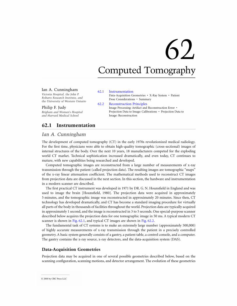
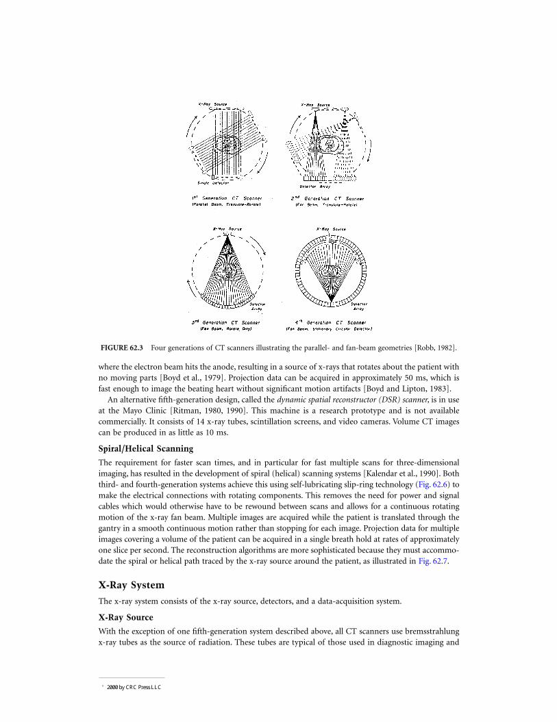
is descried in terms of “generations,” as illustrated in Fig. 62.3, and reflects the historical development

[Newton and Potts, 1981; Seeram, 1994]. Current CT scanners use either third-, fourth-, or fifth-

generation geometries, each having their own pros and cons.

First Generation: Parallel-Beam Geometry

Parallel-beam geometry is the simplest technically and the easiest with which to understand the important

CT principles. Multiple measurements of x-ray transmission are obtained using a single highly collimated

x-ray pencil beam and detector. The beam is translated in a linear motion across the patient to obtain a

projection profile. The source and detector are then rotated about the patient isocenter by approximately

1 degree, and another projection profile is obtained. This translate-rotate scanning motion is repeated

until the source and detector have been rotated by 180 degrees. The highly collimated beam provides

excellent rejection of radiation scattered in the patient; however, the complex scanning motion results

in long (approximately 5-minute) scan times. This geometry was used by Hounsfield in his original

experiments [Hounsfield, 1980] but is not used in modern scanners.

Second Generation: Fan Beam, Multiple Detectors

Scan times were reduced to approximately 30 s with the use of a fan beam of x-rays and a linear detector

array. A translate-rotate scanning motion was still employed; however, a larger rotate increment could

be used, which resulted in shorter scan times. The reconstruction algorithms are slightly more compli-

cated than those for first-generation algorithms because they must handle fan-beam projection data.

Third Generation: Fan Beam, Rotating Detectors

Third-generation scanners were introduced in 1976. A fan beam of x-rays is rotated 360 degrees around

the isocenter. No translation motion is used; however, the fan beam must be wide enough to completely

contain the patient. A curved detector array consisting of several hundred independent detectors is

mechanically coupled to the x-ray source, and both rotate together. As a result, these rotate-only motions

acquire projection data for a single image in as little as 1 s. Third-generation designs have the advantage

that thin tungsten septa can be placed between each detector in the array and focused on the x-ray source

to reject scattered radiation.

FIGURE 62.1 Schematic drawing of a typical CT scanner installation, consisting of (1) control console, (2) gantry

stand, (3) patient table, (4) head holder, and (5) laser imager. (Courtesy of Picker International, Inc.)


Fourth Generation: Fan Beam, Fixed Detectors

In a fourth-generation scanner, the x-ray source and fan beam rotate about the isocenter, while the

detector array remains stationary. The detector array consists of 600 to 4800 (depending on the manu-

facturer) independent detectors in a circle that completely surrounds the patient. Scan times are similar

to those of third-generation scanners. The detectors are no longer coupled to the x-ray source and hence

cannot make use of focused septa to reject scattered radiation. However, detectors are calibrated twice

during each rotation of the x-ray source, providing a self-calibrating system. Third-generation systems

are calibrated only once every few hours.

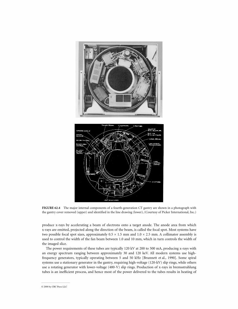
Two detector geometries are currently used for fourth-generation systems: (1) a rotating x-ray source

inside a fixed detector array and (2) a rotating x-ray source outside a nutating detector array. Figure 62.4

shows the major components in the gantry of a typical fourth-generation system using a fixed-detector

array. Both third- and fourth-generation systems are commercially available, and both have been highly

successful clinically. Neither can be considered an overall superior design.

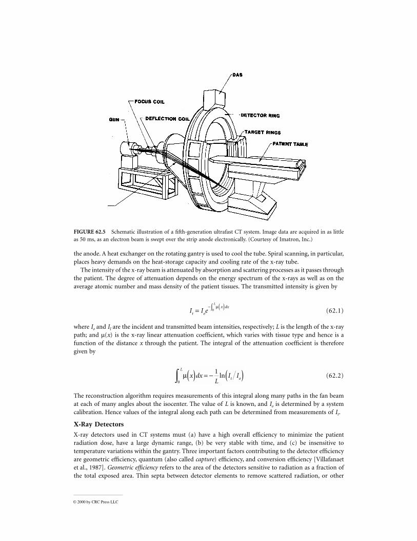
Fifth Generation: Scanning Electron Beam

Fifth-generation scanners are unique in that the x-ray source becomes an integral part of the system

design. The detector array remains stationary, while a high-energy electron beams is electronically swept

along a semicircular tungsten strip anode, as illustrated in Fig. 62.5. X-rays are produced at the point

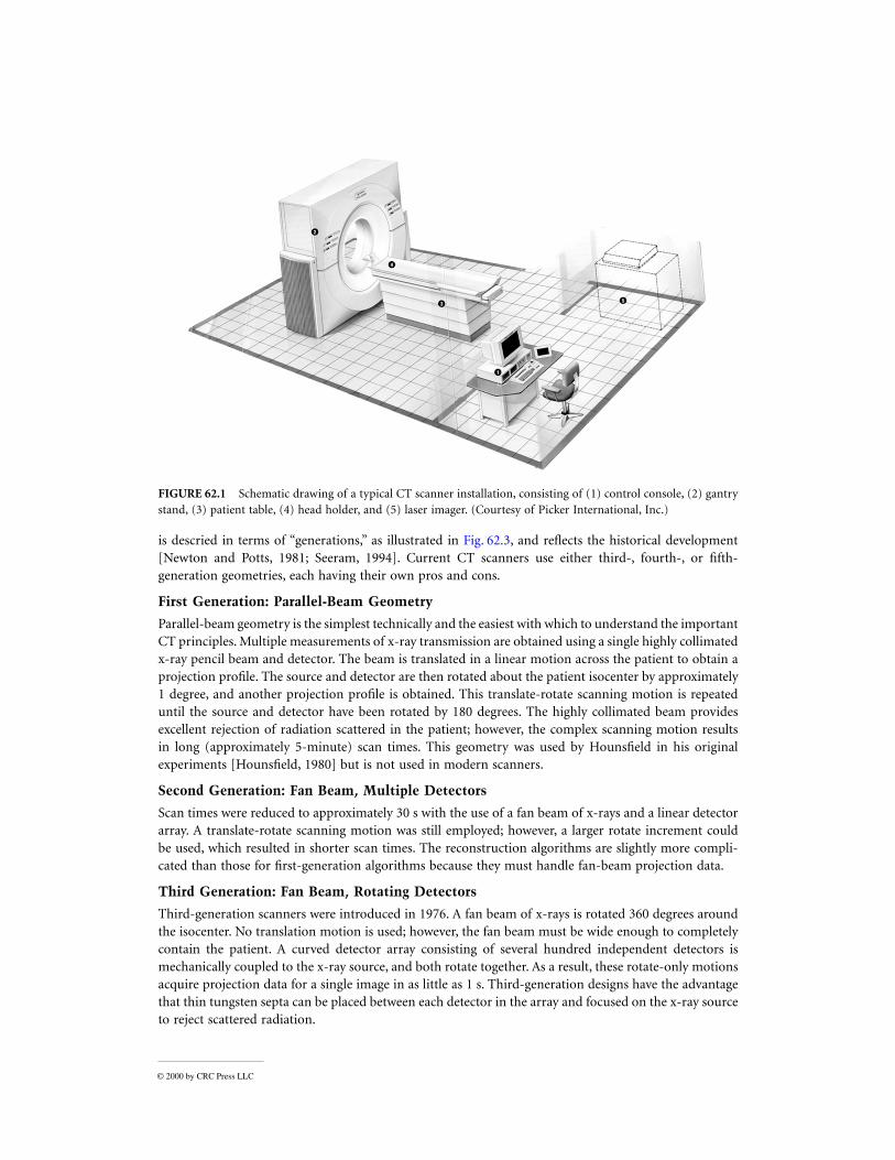
FIGURE 62.2 Typical CT images of (a) brain, (b) head showing orbits, (c) chest showing lungs, and (d) abdomen.

where the electron beam hits the anode, resulting in a source of x-rays that rotates about the patient with

no moving parts [Boyd et al., 1979]. Projection data can be acquired in approximately 50 ms, which is

fast enough to image the beating heart without significant motion artifacts [Boyd and Lipton, 1983].

An alternative fifth-generation design, called the dynamic spatial reconstructor (DSR) scanner, is in use

at the Mayo Clinic [Ritman, 1980, 1990]. This machine is a research prototype and is not available

commercially. It consists of 14 x-ray tubes, scintillation screens, and video cameras. Volume CT images

can be produced in as little as 10 ms.

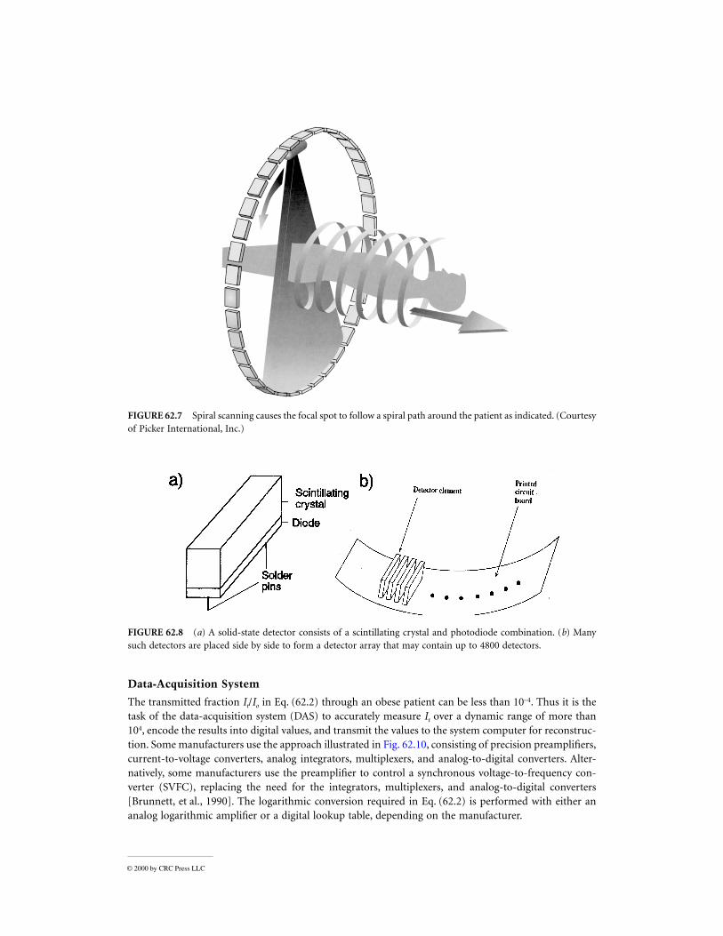
Spiral/Helical Scanning

The requirement for faster scan times, and in particular for fast multiple scans for three-dimensional

imaging, has resulted in the development of spiral (helical) scanning systems [Kalendar et al., 1990]. Both

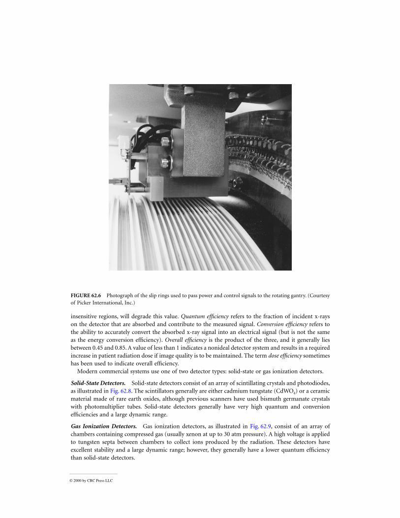
third- and fourth-generation systems achieve this using self-lubricating slip-ring technology (Fig. 62.6) to

make the electrical connections with rotating components. This removes the need for power and signal

cables which would otherwise have to be rewound between scans and allows for a continuous rotating

motion of the x-ray fan beam. Multiple images are acquired while the patient is translated through the

gantry in a smooth continuous motion rather than stopping for each image. Projection data for multiple

images covering a volume of the patient can be acquired in a single breath hold at rates of approximately

one slice per second. The reconstruction algorithms are more sophisticated because they must accommo-

date the spiral or helical path traced by the x-ray source around the patient, as illustrated in Fig. 62.7.

X-Ray System

The x-ray system consists of the x-ray source, detectors, and a data-acquisition system.

X-Ray Source

With the exception of one fifth-generation system described above, all CT scanners use bremsstrahlung

x-ray tubes as the source of radiation. These tubes are typical of those used in diagnostic imaging and

FIGURE 62.3 Four generations of CT scanners illustrating the parallel- and fan-beam geometries [Robb, 1982].



produce x-rays by accelerating a beam of electrons onto a target anode. The anode area from which

x-rays are emitted, projected along the direction of the beam, is called the focal spot. Most systems have

two possible focal spot sizes, approximately 0.5 × 1.5 mm and 1.0 × 2.5 mm. A collimator assembly is

used to control the width of the fan beam between 1.0 and 10 mm, which in turn controls the width of

the imaged slice.

The power requirements of these tubes are typically 120 kV at 200 to 500 mA, producing x-rays with

an energy spectrum ranging between approximately 30 and 120 keV. All modern systems use high-

frequency generators, typically operating between 5 and 50 kHz [Brunnett et al., 1990]. Some spiral

systems use a stationary generator in the gantry, requiring high-voltage (120-kV) slip rings, while others

use a rotating generator with lower-voltage (480-V) slip rings. Production of x-rays in bremsstrahlung

tubes is an inefficient process, and hence most of the power delivered to the tubes results in heating of

FIGURE 62.4 The major internal components of a fourth-generation CT gantry are shown in a photograph with

the gantry cover removed (upper) and identified in the line drawing (lower), (Courtesy of Picker International, Inc.)


the anode. A heat exchanger on the rotating gantry is used to cool the tube. Spiral scanning, in particular,

places heavy demands on the heat-storage capacity and cooling rate of the x-ray tube.

The intensity of the x-ray beam is attenuated by absorption and scattering processes as it passes through

the patient. The degree of attenuation depends on the energy spectrum of the x-rays as well as on the

average atomic number and mass density of the patient tissues. The transmitted intensity is given by

(62.1)

where Io and II are the incident and transmitted beam intensities, respectively; L is the length of the x-ray

path; and µ(x) is the x-ray linear attenuation coefficient, which varies with tissue type and hence is a

function of the distance x through the patient. The integral of the attenuation coefficient is therefore

given by

(62.2)

The reconstruction algorithm requires measurements of this integral along many paths in the fan beam

at each of many angles about the isocenter. The value of L is known, and Io is determined by a system

calibration. Hence values of the integral along each path can be determined from measurements of It.

X-Ray Detectors

X-ray detectors used in CT systems must (a) have a high overall efficiency to minimize the patient

radiation dose, have a large dynamic range, (b) be very stable with time, and (c) be insensitive to

temperature variations within the gantry. Three important factors contributing to the detector efficiency

are geometric efficiency, quantum (also called capture) efficiency, and conversion efficiency [Villafanaet

et al., 1987]. Geometric efficiency refers to the area of the detectors sensitive to radiation as a fraction of

the total exposed area. Thin septa between detector elements to remove scattered radiation, or other

FIGURE 62.5 Schematic illustration of a fifth-generation ultrafast CT system. Image data are acquired in as little

as 50 ms, as an electron beam is swept over the strip anode electronically. (Courtesy of Imatron, Inc.)

I I et o

x dxL

= ∫− µ( )0

µ( ) = − ( )∫ x dxL

I IL

t o0

1ln


insensitive regions, will degrade this value. Quantum efficiency refers to the fraction of incident x-rays

on the detector that are absorbed and contribute to the measured signal. Conversion efficiency refers to

the ability to accurately convert the absorbed x-ray signal into an electrical signal (but is not the same

as the energy conversion efficiency). Overall efficiency is the product of the three, and it generally lies

between 0.45 and 0.85. A value of less than 1 indicates a nonideal detector system and results in a required

increase in patient radiation dose if image quality is to be maintained. The term dose efficiency sometimes

has been used to indicate overall efficiency.

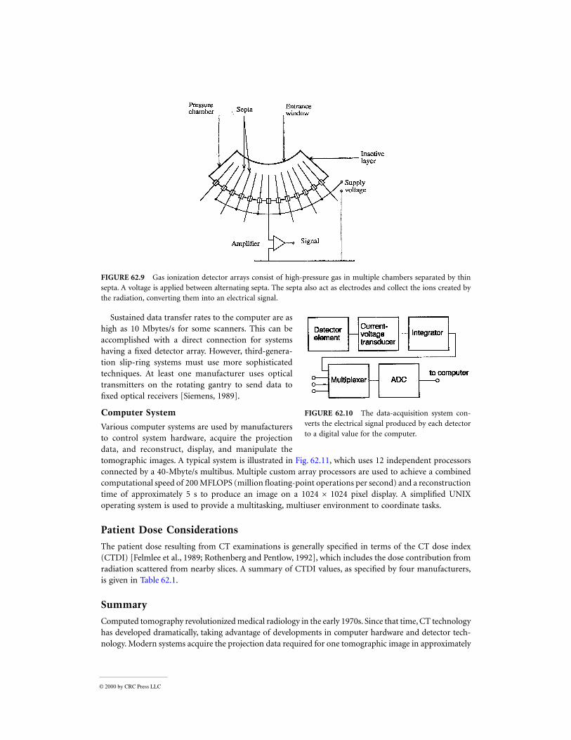
Modern commercial systems use one of two detector types: solid-state or gas ionization detectors.

Solid-State Detectors. Solid-state detectors consist of an array of scintillating crystals and photodiodes,

as illustrated in Fig. 62.8. The scintillators generally are either cadmium tungstate (CdWO4) or a ceramic

material made of rare earth oxides, although previous scanners have used bismuth germanate crystals

with photomultiplier tubes. Solid-state detectors generally have very high quantum and conversion

efficiencies and a large dynamic range.

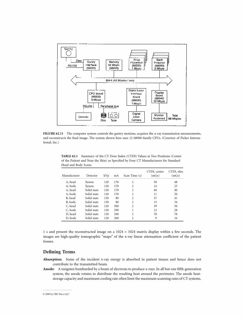
Gas Ionization Detectors. Gas ionization detectors, as illustrated in Fig. 62.9, consist of an array of

chambers containing compressed gas (usually xenon at up to 30 atm pressure). A high voltage is applied

to tungsten septa between chambers to collect ions produced by the radiation. These detectors have

excellent stability and a large dynamic range; however, they generally have a lower quantum efficiency

than solid-state detectors.

FIGURE 62.6 Photograph of the slip rings used to pass power and control signals to the rotating gantry. (Courtesy

of Picker International, Inc.)


Data-Acquisition System

The transmitted fraction It/Io in Eq. (62.2) through an obese patient can be less than 10–4. Thus it is the

task of the data-acquisition system (DAS) to accurately measure It over a dynamic range of more than

104, encode the results into digital values, and transmit the values to the system computer for reconstruc-

tion. Some manufacturers use the approach illustrated in Fig. 62.10, consisting of precision preamplifiers,

current-to-voltage converters, analog integrators, multiplexers, and analog-to-digital converters. Alter-

natively, some manufacturers use the preamplifier to control a synchronous voltage-to-frequency con-

verter (SVFC), replacing the need for the integrators, multiplexers, and analog-to-digital converters

[Brunnett, et al., 1990]. The logarithmic conversion required in Eq. (62.2) is performed with either an

analog logarithmic amplifier or a digital lookup table, depending on the manufacturer.

FIGURE 62.7 Spiral scanning causes the focal spot to follow a spiral path around the patient as indicated. (Courtesy

of Picker International, Inc.)

FIGURE 62.8 (a) A solid-state detector consists of a scintillating crystal and photodiode combination. (b) Many

such detectors are placed side by side to form a detector array that may contain up to 4800 detectors.


Sustained data transfer rates to the computer are as

high as 10 Mbytes/s for some scanners. This can be

accomplished with a direct connection for systems

having a fixed detector array. However, third-genera-

tion slip-ring systems must use more sophisticated

techniques. At least one manufacturer uses optical

transmitters on the rotating gantry to send data to

fixed optical receivers [Siemens, 1989].

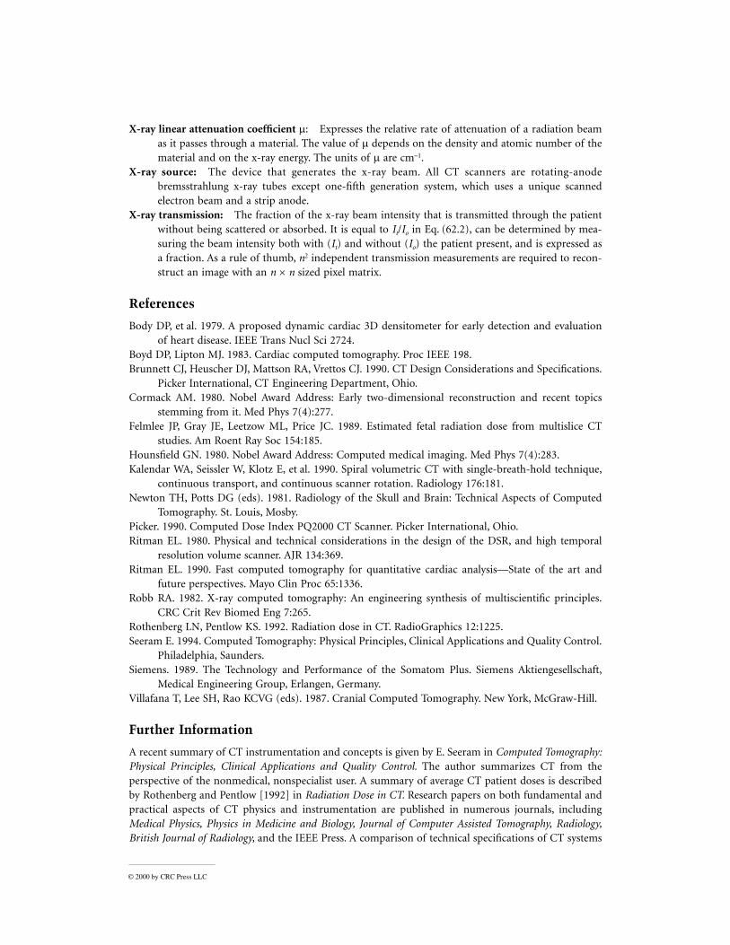
Computer System

Various computer systems are used by manufacturers

to control system hardware, acquire the projection

data, and reconstruct, display, and manipulate the

tomographic images. A typical system is illustrated in Fig. 62.11, which uses 12 independent processors

connected by a 40-Mbyte/s multibus. Multiple custom array processors are used to achieve a combined

computational speed of 200 MFLOPS (million floating-point operations per second) and a reconstruction

time of approximately 5 s to produce an image on a 1024 × 1024 pixel display. A simplified UNIX

operating system is used to provide a multitasking, multiuser environment to coordinate tasks.

Patient Dose Considerations

The patient dose resulting from CT examinations is generally specified in terms of the CT dose index

(CTDI) [Felmlee et al., 1989; Rothenberg and Pentlow, 1992], which includes the dose contribution from

radiation scattered from nearby slices. A summary of CTDI values, as specified by four manufacturers,

is given in Table 62.1.

Summary

Computed tomography revolutionized medical radiology in the early 1970s. Since that time, CT technology

has developed dramatically, taking advantage of developments in computer hardware and detector tech-

nology. Modern systems acquire the projection data required for one tomographic image in approximately

FIGURE 62.9 Gas ionization detector arrays consist of high-pressure gas in multiple chambers separated by thin

septa. A voltage is applied between alternating septa. The septa also act as electrodes and collect the ions created by

the radiation, converting them into an electrical signal.

FIGURE 62.10 The data-acquisition system con-

verts the electrical signal produced by each detector

to a digital value for the computer.


1 s and present the reconstructed image on a 1024 × 1024 matrix display within a few seconds. The

images are high-quality tomographic “maps” of the x-ray linear attenuation coefficient of the patient

tissues.

Defining Terms

Absorption: Some of the incident x-ray energy is absorbed in patient tissues and hence does not

contribute to the transmitted beam.

Anode: A tungsten bombarded by a beam of electrons to produce x-rays. In all but one fifth-generation

system, the anode rotates to distribute the resulting heat around the perimeter. The anode heat-

storage capacity and maximum cooling rate often limit the maximum scanning rates of CT systems.

FIGURE 62.11 The computer system controls the gantry motions, acquires the x-ray transmission measurements,

and reconstructs the final image. The system shown here uses 12 68000-family CPUs. (Courtesy of Picker Interna-

tional, Inc.)

TABLE 62.1 Summary of the CT Dose Index (CTDI) Values at Two Positions (Center

of the Patient and Near the Skin) as Specified by Four CT Manufacturers for Standard

Head and Body Scans.

CTDI, center CTDI, skin

Manufacturer Detector kVp mA Scan Time (s) (mGy) (mGy)

A, head Xenon 120 170 2 50 48

A, body Xenon 120 170 2 14 25

A, head Solid state 120 170 2 40 40

A, body Solid state 120 170 2 11 20

B, head Solid state 130 80 2 37 41

B, body Solid state 130 80 2 15 34

C, head Solid state 120 500 2 39 50

C, body Solid state 120 290 1 12 28

D, head Solid state 120 200 2 78 78

D, body Solid state 120 200 2 9 16


Attenuation: The total decrease in the intensity of the primary x-ray beam as it passes through the

patient, resulting from both scatter and absorption processes. It is characterized by the linear

attenuation coefficient.

Computed tomography (CT): A computerized method of producing x-ray tomographic images. Pre-

vious names for the same thing include computerized tomographic imaging, computerized axial

tomography (CAT), computer-assisted tomography (CAT), and reconstructive tomography (RT).

Control console: The control console is used by the CT operator to control the scanning operations,

image reconstruction, and image display.

Cormack, Dr. Allan MacLeod: A physicist who developed mathematical techniques required in the

reconstruction of tomographic images. Dr. Cormack shared the Nobel Prize in Medicine and

Physiology with Dr. G. N. Hounsfield in 1979 [Cormack, 1980].

Data-acquisition system (DAS): Interfaces the x-ray detectors to the system computer and may consist

of a preamplifier, integrator, multiplexer, logarithmic amplifier, and analog-to-digital converter.

Detector array: An array of individual detector elements. The number of detector elements varies

between a few hundred and 4800, depending on the acquisition geometry and manufacturer. Each

detector element functions independently of the others.

Fan beam: The x-ray beam is generated at the focal spot and so diverges as it passes through the patient

to the detector array. The thickness of the beam is generally selectable between 1.0 and 10 mm

and defines the slice thickness.

Focal spot: The region of the anode where x-rays are generated.

Focused septa: Thin metal plates between detector elements which are aligned with the focal spot so

that the primary beam passes unattenuated to the detector elements, while scattered x-rays which

normally travel in an altered direction are blocked.

Gantry: The largest component of the CT installation, containing the x-ray tube, collimators, detector

array, DAS, other control electronics, and the mechanical components required for the scanning

motions.

Helical scanning: The scanning motions in which the x-ray tube rotates continuously around the

patient while the patient is continuously translated through the fan beam. The focal spot therefore

traces a helix around the patient. Projection data are obtained which allow the reconstruction of

multiple contiguous images. This operation is sometimes called spiral, volume, or three-dimensional

CT scanning.

Hounsfield, Dr. Godfrey Newbold: An engineer who developed the first practical CT instrument in

1971. Dr. Hounsfield received the McRobert Award in 1972 and shared the Nobel Prize in Medicine

and Physiology with Dr. A. M. Cormack in 1979 for this invention [Hounsfield, 1980].

Image plane: The plane through the patient that is imaged. In practice, this plane (also called a slice)

has a selectable thickness between 1.0 and 10 mm centered on the image plane.

Pencil beam: A narrow, well-collimated beam of x-rays.

Projection data: The set of transmission measurements used to reconstruct the image.

Reconstruct: The mathematical operation of generating the tomographic image from the projection

data.

Scan time: The time required to acquire the projection data for one image, typically 1.0 s.

Scattered radiation: Radiation that is removed from the primary beam by a scattering process. This

radiation is not absorbed but continues along a path in an altered direction.

Slice: See Image plane.

Spiral scanning: See Helical scanning.

Three-dimensional imaging: See Helical scanning.

Tomography: A technique of imaging a cross-sectional slice.

Volume CT: See Helical scanning.

X-ray detector: A device that absorbs radiation and converts some or all of the absorbed energy into

a small electrical signal.


X-ray linear attenuation coefficient µ: Expresses the relative rate of attenuation of a radiation beam

as it passes through a material. The value of µ depends on the density and atomic number of the

material and on the x-ray energy. The units of µ are cm–1.

X-ray source: The device that generates the x-ray beam. All CT scanners are rotating-anode

bremsstrahlung x-ray tubes except one-fifth generation system, which uses a unique scanned

electron beam and a strip anode.

X-ray transmission: The fraction of the x-ray beam intensity that is transmitted through the patient

without being scattered or absorbed. It is equal to It/Io in Eq. (62.2), can be determined by mea-

suring the beam intensity both with (It) and without (Io) the patient present, and is expressed as

a fraction. As a rule of thumb, n2 independent transmission measurements are required to recon-

struct an image with an n × n sized pixel matrix.

References

Body DP, et al. 1979. A proposed dynamic cardiac 3D densitometer for early detection and evaluation

of heart disease. IEEE Trans Nucl Sci 2724.

Boyd DP, Lipton MJ. 1983. Cardiac computed tomography. Proc IEEE 198.

Brunnett CJ, Heuscher DJ, Mattson RA, Vrettos CJ. 1990. CT Design Considerations and Specifications.

Picker International, CT Engineering Department, Ohio.

Cormack AM. 1980. Nobel Award Address: Early two-dimensional reconstruction and recent topics

stemming from it. Med Phys 7(4):277.

Felmlee JP, Gray JE, Leetzow ML, Price JC. 1989. Estimated fetal radiation dose from multislice CT

studies. Am Roent Ray Soc 154:185.

Hounsfield GN. 1980. Nobel Award Address: Computed medical imaging. Med Phys 7(4):283.

Kalendar WA, Seissler W, Klotz E, et al. 1990. Spiral volumetric CT with single-breath-hold technique,

continuous transport, and continuous scanner rotation. Radiology 176:181.

Newton TH, Potts DG (eds). 1981. Radiology of the Skull and Brain: Technical Aspects of Computed

Tomography. St. Louis, Mosby.

Picker. 1990. Computed Dose Index PQ2000 CT Scanner. Picker International, Ohio.

Ritman EL. 1980. Physical and technical considerations in the design of the DSR, and high temporal

resolution volume scanner. AJR 134:369.

Ritman EL. 1990. Fast computed tomography for quantitative cardiac analysis—State of the art and

future perspectives. Mayo Clin Proc 65:1336.

Robb RA. 1982. X-ray computed tomography: An engineering synthesis of multiscientific principles.

CRC Crit Rev Biomed Eng 7:265.

Rothenberg LN, Pentlow KS. 1992. Radiation dose in CT. RadioGraphics 12:1225.

Seeram E. 1994. Computed Tomography: Physical Principles, Clinical Applications and Quality Control.

Philadelphia, Saunders.

Siemens. 1989. The Technology and Performance of the Somatom Plus. Siemens Aktiengesellschaft,

Medical Engineering Group, Erlangen, Germany.

Villafana T, Lee SH, Rao KCVG (eds). 1987. Cranial Computed Tomography. New York, McGraw-Hill.

Further Information

A recent summary of CT instrumentation and concepts is given by E. Seeram in Computed Tomography:

Physical Principles, Clinical Applications and Quality Control. The author summarizes CT from the

perspective of the nonmedical, nonspecialist user. A summary of average CT patient doses is described

by Rothenberg and Pentlow [1992] in Radiation Dose in CT. Research papers on both fundamental and

practical aspects of CT physics and instrumentation are published in numerous journals, including

Medical Physics, Physics in Medicine and Biology, Journal of Computer Assisted Tomography, Radiology,

British Journal of Radiology, and the IEEE Press. A comparison of technical specifications of CT systems


provided by the manufacturers is available from ECRI to help orient the new purchaser in a selection

process. Their Product Comparison System includes a table of basic specifications for all the major

international manufactures.

62.2 Reconstruction Principles

Philip F. Judy

Computed tomography (CT) is a two-step process: (1) the transmission of an x-ray beam is measured

through all possible straight-line paths as in a plane of an object, and (2) the attenuation of an x-ray

beam is estimated at points in the object. Initially, the transmission measurements will be assumed to

be the results of an experiment performed with a narrow monoenergetic beam of x-rays that are confined

to a plane. The designs of devices that attempt to realize these measurements are described in the

preceding section. One formal consequence of these assumptions is that the logarithmic transformation

of the measured x-ray intensity is proportional to the line integral of attenuation coefficients. In order

to satisfy this assumption, computer processing procedures on the measurements of x-ray intensity are

necessary even before image reconstruction is performed. These linearization procedures will reviewed

after background.

Both analytical and iterative estimations of linear x-ray attenuation have been used for transmission

CT reconstruction. Iterative procedures are of historic interest because an iterative reconstruction pro-

cedure was used in the first commercially successful CT scanner [EMI, Mark I, Hounsfield, 1973]. They

also permit easy incorporation of physical processes that cause deviations from the linearity. Their

practical usefulness is limited. The first EMI scanner required 20 minutes to finish its reconstruction.

Using the identical hardware and employing an analytical calculation, the estimation of attenuation values

was performed during the 4.5-minute data acquisition and was made on a 160 × 160 matrix. The original

iterative procedure reconstructed the attenuation values on an 80 × 80 matrix and consequently failed

to exploit all the spatial information inherent in transmission data.

Analytical estimation, or direct reconstruction, uses a numerical approximation of the inverse Radon

transform [Radon, 1917]. The direct reconstruction technique (convolution-backprojection) presently

used in x-ray CT was initially applied in other areas such as radio astronomy [Bracewell and Riddle,

1967] and electron microscopy [Crowther et al., 1970; Ramachandran and Lakshminarayana, 1971].

These investigations demonstrated that the reconstructions from the discrete spatial sampling of band-

limited data led to full recovery of the cross-sectional attenuation. The random variation (noise) in x-ray

transmission measurements may not be bandlimited. Subsequent investigators [e.g., Chesler and Riederer,

1975; Herman and Roland, 1973; Shepp and Logan, 1974] have suggested various bandlimiting windows

that reduce the propagation and amplification of noise by the reconstruction. These issues have been

investigated by simulation, and investigators continue to pursue these issues using a computer phantom

[e.g., Guedon and Bizais, 1994, and references therein] described by Shepp and Logan. The subsequent

investigations of the details of choice of reconstruction parameters has had limited practical impact

because real variation of transmission data is bandlimited by the finite size of the focal spot and radiation

detector, a straightforward design question, and because random variation of the transmission tends to

be uncorrelated. Consequently, the classic precedures suffice.

Image Processing: Artifact and Reconstruction Error

An artifact is a reconstruction defect that is obviously visible in the image. The classification of an image

feature as an artifact involves some visual criterion. The effect must produce an image feature that is

greater than the random variation in image caused by the intrinsic variation in transmission measure-

ments. An artifact not recognized by the physician observer as an artifact may be reported as a lesion.

Such false-positive reports could lead to an unnecessary medical procedure, e.g., surgery to remove an

imaginary tumor. A reconstruction error is a deviation of the reconstruction value from its expected value.


Reconstruction errors are significant if the application involves a quantitative measurement, not a com-

mon medical application. The reconstruction errors are characterized by identical material at different

points in the object leading to different reconstructed attenuation values in the image which are not

visible in the medical image.

Investigators have used computer simulation to investigate artifact [Herman, 1980] because image

noise limits the visibility of their visibility. One important issue investigated was required spatial sampling

of transmission slice plane [Crawford and Kak, 1979; Parker et al., 1982]. These simulations provided a

useful guideline in design. In practice, these aliasing artifacts are overwhelmed by random noise, and

designers tend to oversample in the slice plane. A second issue that was understood by computer

simulation was the partial volume artifact [Glover and Pelc, 1980]. This artifact would occur even for

mononergetic beams and finite beam size, particularly in the axial dimension. The axial dimension of

the beams tend to be greater (about 10 mm) than their dimensions in the slice plane (about 1 mm). The

artifact is created when the variation of transmission within the beam varies considerably, and the

exponential variation within the beam is summed by the radiation detector. The logarithm transforma-

tion of the detected signal produces a nonlinear effect that is propagated throughout the image by the

reconstruction process. Simulation was useful in demonstrating that isolated features in the same cross-

section act together to produce streak artifacts. Simulations have been useful to illustrate the effects of

patient motion during the data-acquisition streaks off high-contrast objects.

Projection Data to Image: Calibrations

Processing of transmission data is necessary to obtain high-quality images. In general, optimization of

the projection data will optimize the reconstructed image. Reconstruction is a process that removes the

spatial correlation of attenuation effects in the transmitted image by taking advantage of completely

sampling the possible transmissions. Two distinct calibrations are required: registration of beams with

the reconstruction matrix and linearization of the measured signal.

Without loss of generalization, a projection will be considered a set of transmissions made along

parallel lines in the slice plane of the CT scanner. Without loss of generalization means that essential

aspects of all calibration and reconstruction procedures required for fan-beam geometries are captured

by the calibration and reconstruction procedures described for parallel projections. One line of each

projection is assumed to pass through the center of rotation of data collection. Shepp et al. [1979] showed

that errors in the assignment of that center-of-rotation point in the projections could lead to considerable

distinctive artifacts and that small errors (0.05 mm) would produce these effects. The consequences of

these errors have been generalized to fan-beam collection schemes, and images reconstructed from 180-

degree projection sets were compared with images reconstructed from 360-degree data sets [Kijewski

and Judy, 1983]. A simple misregistration of the center of rotation was found to produce blurring of

image without the artifact. These differences may explain the empirical observation that most commercial

CT scanners collect a full 360-degree data set even though 180 degrees of data will suffice.

The data-acquisition scheme that was designed to overcome the limited sampling inherent in third-

generation fan-beam systems by shifting detectors a quarter sampling distance while opposite 180-degree

projection is measured, has particularly stringent registration requirements. Also, the fourth-generation

scanner does not link the motion of the x-ray tube and the detector; consequently, the center of rotation

is determined as part of a calibration procedure, and unsystematic effects lead to artifacts that mimic

noise besides blurring the image.

Misregistration artifacts also can be mitigated by feathering. This procedure requires collection of

redundant projection data at the end of the scan. A single data set is produced by linearly weighting the

redundant data at the beginning and end of the data collection [Parker et al., 1982]. These procedures

have be useful in reducing artifacts from gated data collections [Moore et al., 1987].

The other processing necessary before reconstruction of project data is linearization. The formal require-

ment for reconstruction is that the line integrals of some variable be available; this is the variable that

ultimately is reconstructed. The logarithm of x-ray transmission approximates this requirement. There


are physical effects in real x-ray transmissions that cause deviations from this assumption. X-ray beams

of sufficient intensity are composed of photons of different energies. Some photons in the beam interact

with objects and are scattered rather than absorbed. The spectrum of x-ray photons of different attenuation

coefficients means the logarithm of the transmission measurement will not be proportional to the line

integral of the attenuation coefficient along that path, because an attenuation coefficient cannot even be

defined. An effective attenuation coefficient can only be defined uniquely for a spectrum for a small mass

of material that alters that intensity. It has to be small enough not to alter the spectrum [McCullough, 1979].

A straightforward approach to this nonunique attenuation coefficient error, called hardening, is to

assume that the energy dependence of the attenuation coefficient is constant and that differences in

attenuation are related to a generalized density factor that multiplies the spectral dependence of attenu-

ation. The transmission of an x-ray beam then can be estimated for a standard material, typically water,

as a function of thickness. This assumption is that attenuations of materials in the object, the human

body, differ because specific gravities of the materials differ. Direct measurements of the transmission of

an actual x-ray beam may provide initial estimates that can be parameterized. The inverse of this function

provides the projection variable that is reconstructed. The parameters of the function are usually modified

as part of a calibration to make the CT image of a uniform water phantom flat.

Such a calibration procedure does not deal completely with the hardening effects. The spectral depen-

dence of bone differs considerably from that of water. This is particularly critical in imaging of the brain,

which is contained within the skull. Without additional correction, the attenuation values of brain are

lower in the center than near the skull.

The detection of scattered energy means that the reconstructed attenuation coefficient will differ from

the attenuation coefficient estimated with careful narrow-beam measurements. The x-rays appear more

penetrating because scattered x-rays are detected. The zero-ordered scatter, a decrease in the attenuation

coefficient by some constant amount, is dealt with automatically by the calibration that treats hardening.

First-order scattering leads to a widening of the x-ray beam and can be dealt with by a modification of

the reconstruction kernel.

Projection Data to Image: Reconstruction

The impact of CT created considerable interest in the formal aspects of reconstruction. There are many

detailed descriptions of direct reconstruction procedures. Some are presented in textbooks used in

graduate courses for medical imaging [Barrett and Swindell, 1981; Cho et al., 1993]. Herman (1980)

published a textbook that was based on a two-semester course that dealt exclusively with reconstruction

principles, demonstrating the reconstruction principles with simulation.

The standard reconstruction method is called convolution-backprojection. The first step in the proce-

dure is to convolve the projection, a set of transmissions made along parallel lines in the slice plane, with

a reconstruction kernel derived from the inverse Radon transform. The choice of kernel is dictated by

bandlimiting issues [Chesler and Riederer, 1975; Herman and Roland, 1973; Shepp and Logan, 1974]. It

can be modified to deal with the physical aperture of the CT system [Bracewell, 1977], which might

include the effects of scatter. The convolved projection is then backprojected onto a two-dimensional

image matrix. Backprojection is the opposite of projection; the value of the projection is added to each

point along the line of the projection. This procedure makes sense in the continuous description, but in

the discrete world of the computer, the summation is done over the image matrix.

Consider a point of the image matrix; very few, possibly no lines of the discrete projection data intersect

the point. Consequently, to estimate the projection value to be added to that point, the procedure must

interpolate between two values of sampled convolve projection. The linear interpolation scheme is a

significant improvement over nearest project nearest to the point. More complex schemes get confounded

with choices of reconstruction kernel, which are designed to accomplish standard image processing in

the image, e.g., edge enhancement.

Scanners have been developed to acquire a three-dimensional set of projection data [Kalender et al.,

1990]. The motion of the source defines a spiral motion relative to the patient. The spiral motion defines


an axis. Consequently, only one projection is available for reconstruction of the attenuation values in the

plane. This is the back-projection problem just discussed; no correct projection value is available from

the discrete projection data set. The solution is identical: a projection value is interpolated from the

existing projection values to estimate the necessary projections for each plane to be reconstructed. This

procedure has the advantage that overlapping slices can be reconstructed without additional exposure,

and this eliminates the risk that a small lesion will be missed because it straddles adjacent slices. This

data-collection scheme is possible because systems that continuously rotate have been developed. The

spiral scan motion is realized by moving the patient through the gantry. Spiral CT scanners have made

possible the acquisition of an entire data set in a single breath hold.

References

Barrett HH, Swindell W. 1981. Radiological Imaging: The Theory and Image Formation, Detection, and

Processing, vol 2. New York, Academic Press.

Bracewell RN, Riddle AC. 1976. Inversion of fan-beam scans in radio astronomy. The Astrophysical

Journal 150:427-434.

Chesler DA, Riederer SJ. 1975. Ripple suppression during reconstruction in transverse tomography. Phys

Med Biol 20(4):632-636.

Cho Z, Jones JP, Singh M. 1993. Foundations of medical imaging. New York, Wiley & Sons, Inc.

Crawford CR, Kak AC. 1979. Aliasing artifacts in computerized tomography. Applied Optics 18:3704-3711.

Glover GH, Pelc NJ. 1980. Nonlinear partial volume artifacts in x-ray computed tomography. Med Phys

7:238-248.

Guedon J-P, Bizais. 1994. Bandlimited and harr filtered back-projection reconstruction. IEEE Trans

Medical Imaging 13(3):430-440.

Herman GT, Rowland SW. 1973. Three methods for reconstruction objects for x-rays—a comparative

study. Comp Graph Imag Process 2:151–178.

Herman GT. 1980. Image Reconstruction from Projection: The Fundamentals of Computerized Tomog-

raphy. New York, New York, Academic Press.

Hounsfield, GN. 1973. Computerized transverse axial scanning (tomography): Part I. Brit J Radiol

46:1016–1022.

Kalender WA, Weissler, Klotz E, et al. 1990. Spiral volumetric CT with single-breath-hold technique,

continuous transport, and continuous scanner rotation. Radiology 176:181–183.

Kijewski MF, Judy PF. 1983. The effect of misregistration of the projections on spatial resolution of CT

scanners. Med Phys 10:169–175.

McCullough EC. 1979. Specifying and evaluating the performance of computed tomographic (CT)

scanners. Med Phys 7:291–296.

Moore SC, Judy PF, Garnic JD, et al. 1983. The effect of misregistration of the projections on spatial

resolution of CT scanners. Med Phys 10:169–175.

Documents

Computed Tomography - k-Space.orgk-space.org/ymk/CT_ch062.pdf · Computed Tomography ... For the ﬁrst time, physicians were able to obtain high-quality tomographic (cross-sectional)