Embed Size (px)
Citation preview
May 2015 Computer Arithmetic, Real Arithmetic Slide 1
Part VReal Arithmetic
Number Representation Numbers and Arithmetic Representing Signed Numbers Redundant Number Systems Residue Number Systems
Addition / Subtraction Basic Addition and Counting Carry-Lookahead Adders Variations in Fast Adders Multioperand Addition
Multiplication Basic Multiplication Schemes High-Radix Multipliers Tree and Array Multipliers Variations in Multipliers
Division Basic Division Schemes High-Radix Dividers Variations in Dividers Division by Convergence
Real Arithmetic Floating-Point Reperesentations Floating-Point Operations Errors and Error Control Precise and Certifiable Arithmetic
Function Evaluation Square-Rooting Methods The CORDIC Algorithms Variations in Function Evaluation Arithmetic by Table Lookup
Implementation Topics High-Throughput Arithmetic Low-Power Arithmetic Fault-Tolerant Arithmetic Past, Present, and Future
Parts Chapters
I.
II.
III.
IV.
V.
VI.
VII.
1. 2. 3. 4.
5. 6. 7. 8.
9. 10. 11. 12.
25. 26. 27. 28.
21. 22. 23. 24.
17. 18. 19. 20.
13. 14. 15. 16.
Ele
men
tary
Ope
ratio
ns
28. Reconfigurable Arithmetic
Appendix: Past, Present, and Future
May 2015 Computer Arithmetic, Real Arithmetic Slide 2
About This Presentation
Edition Released Revised Revised Revised RevisedFirst Jan. 2000 Sep. 2001 Sep. 2003 Oct. 2005 May 2007
May 2008 May 2009
Second May 2010 Apr. 2011 May 2012 May 2015
This presentation is intended to support the use of the textbook Computer Arithmetic: Algorithms and Hardware Designs (Oxford U. Press, 2nd ed., 2010, ISBN 978-0-19-532848-6). It is updated regularly by the author as part of his teaching of the graduate course ECE 252B, Computer Arithmetic, at the University of California, Santa Barbara. Instructors can use these slides freely in classroom teaching and for other educational purposes. Unauthorized uses are strictly prohibited. © Behrooz Parhami
May 2015 Computer Arithmetic, Real Arithmetic Slide 3
V Real Arithmetic
Topics in This PartChapter 17 Floating-Point RepresentationsChapter 18 Floating-Point OperationsChapter 19 Errors and Error ControlChapter 20 Precise and Certifiable Arithmetic
Review floating-point numbers, arithmetic, and errors:• How to combine wide range with high precision• Format and arithmetic ops; the IEEE standard• Causes and consequence of computation errors• When can we trust computation results?

May 2015 Computer Arithmetic, Real Arithmetic Slide 4
“According to my calculation, you should float now ... I think ...” “It’s an inexact science.”
May 2015 Computer Arithmetic, Real Arithmetic Slide 5
17 Floating-Point Representations
Chapter GoalsStudy a representation method offering bothwide range (e.g., astronomical distances)and high precision (e.g., atomic distances)
Chapter HighlightsFloating-point formats and related tradeoffsThe need for a floating-point standardFiniteness of precision and rangeFixed-point and logarithmic representations
as special cases at the two extremes
May 2015 Computer Arithmetic, Real Arithmetic Slide 6
Floating-Point Representations: Topics
Topics in This Chapter
17.1 Floating-Point Numbers
17.2 The IEEE Floating-Point Standard
17.3 Basic Floating-Point Algorithms
17.4 Conversions and Exceptions
17.5 Rounding Schemes
17.6 Logarithmic Number Systems
May 2015 Computer Arithmetic, Real Arithmetic Slide 7
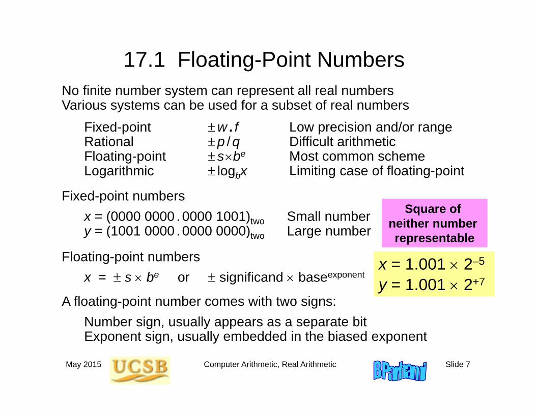
17.1 Floating-Point NumbersNo finite number system can represent all real numbersVarious systems can be used for a subset of real numbers
Fixed-point w . fRational p /qFloating-point sbe
Logarithmic logbx
Fixed-point numbersx = (0000 0000 .0000 1001)two Small numbery = (1001 0000 .0000 0000)two Large number
Low precision and/or rangeDifficult arithmeticMost common schemeLimiting case of floating-point
Floating-point numbersx = s be or significand baseexponent
A floating-point number comes with two signs: Number sign, usually appears as a separate bit Exponent sign, usually embedded in the biased exponent
Square of neither number representable
x = 1.001 2–5
y = 1.001 2+7
May 2015 Computer Arithmetic, Real Arithmetic Slide 8
Floating-Point Number Format and Distribution
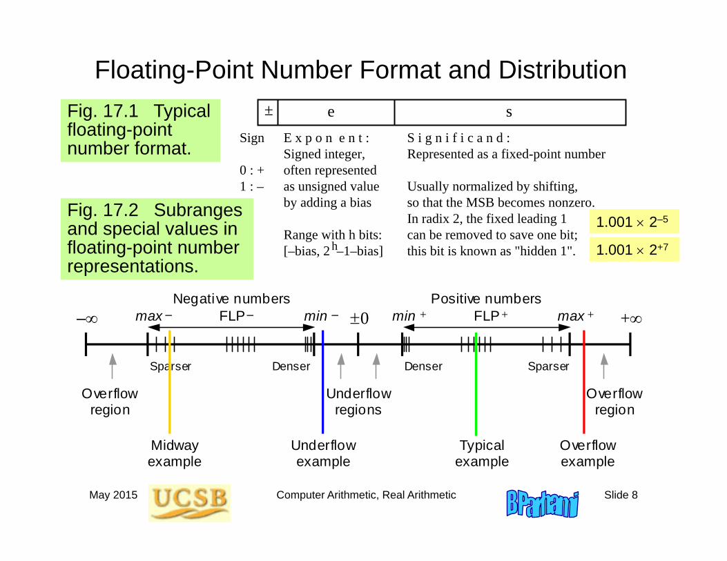
Fig. 17.2 Subranges and special values in floating-point number representations.
E x p o n e n t : Signed integer, often represented as unsigned value by adding a bias Range with h bits: [–bias, 2 –1–bias]h
S i g n i f i c a n d : Represented as a fixed-point number
Usually normalized by shifting, so that the MSB becomes nonzero. In radix 2, the fixed leading 1 can be removed to save one bit; this bit is known as "hidden 1".
Sign 0 : + 1 : –
± e sFig. 17.1 Typical floating-point number format.
Denser Denser Sparser Sparser
Negative numbers FLP FLP 0 +
–
Overflow region
Overflow region
Underflow regions
Positive numbers
Underflow example
Overflow example
Midway example
Typical example
min max min max + + – – – +
1.001 2–5
1.001 2+7

May 2015 Computer Arithmetic, Real Arithmetic Slide 9
Floating-Point Before the IEEE StandardComputer manufacturers tended to have their own hardware-level formats
This created many problems, as floating-point computations could produce vastly different results (not just differing in the last few significant bits)
In computer arithmetic, we talked about IBM, CDC, DEC, Cray, … formats and discussed their relative merits
First IEEE standard for binary floating-point arithmetic was adopted in 1985 after years of discussion
The 1985 standard was continuously discussed, criticized, and clarified for a couple of decades
In 2008, after several years of discussion, a revised standard was issued
To get a sense for the wide variations in floating-point formats, visit:
http://www.mrob.com/pub/math/floatformats.html
May 2015 Computer Arithmetic, Real Arithmetic Slide 10
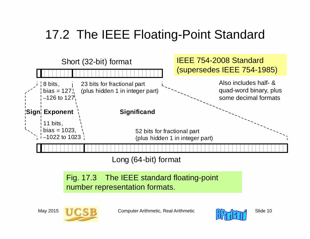
17.2 The IEEE Floating-Point Standard
Short (32-bit) format
Long (64-bit) format
Sign Exponent Significand
8 bits, bias = 127, –126 to 127
11 bits, bias = 1023, –1022 to 1023
52 bits for fractional part (plus hidden 1 in integer part)
23 bits for fractional part (plus hidden 1 in integer part)
Fig. 17.3 The IEEE standard floating-point number representation formats.
IEEE 754-2008 Standard(supersedes IEEE 754-1985)
Also includes half- & quad-word binary, plus some decimal formats
May 2015 Computer Arithmetic, Real Arithmetic Slide 11
Overview of IEEE 754-2008 Standard Formats
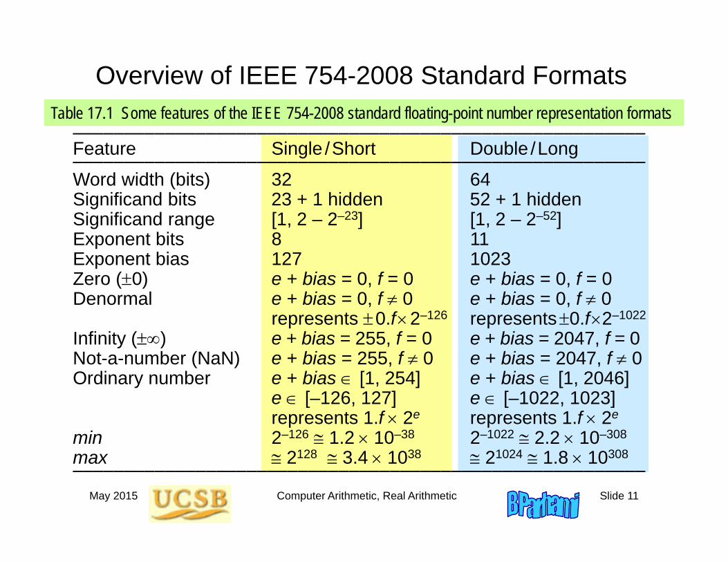
––––––––––––––––––––––––––––––––––––––––––––––––––––––––Feature Single /Short Double /Long––––––––––––––––––––––––––––––––––––––––––––––––––––––––Word width (bits) 32 64Significand bits 23 + 1 hidden 52 + 1 hiddenSignificand range [1, 2 – 2–23] [1, 2 – 2–52]Exponent bits 8 11Exponent bias 127 1023Zero (0) e + bias = 0, f = 0 e + bias = 0, f = 0Denormal e + bias = 0, f 0 e + bias = 0, f 0
represents 0.f2–126 represents0.f2–1022
Infinity () e + bias = 255, f = 0 e + bias = 2047, f = 0Not-a-number (NaN) e + bias = 255, f 0 e + bias = 2047, f 0Ordinary number e + bias [1, 254] e + bias [1, 2046]
e [–126, 127] e [–1022, 1023]represents 1.f 2e represents 1.f 2e
min 2–126 1.2 10–38 2–1022 2.2 10–308
max 2128 3.4 1038 21024 1.8 10308––––––––––––––––––––––––––––––––––––––––––––––––––––––––
Table 17.1 Some features of the IEEE 754-2008 standard floating-point number representation formats
May 2015 Computer Arithmetic, Real Arithmetic Slide 12
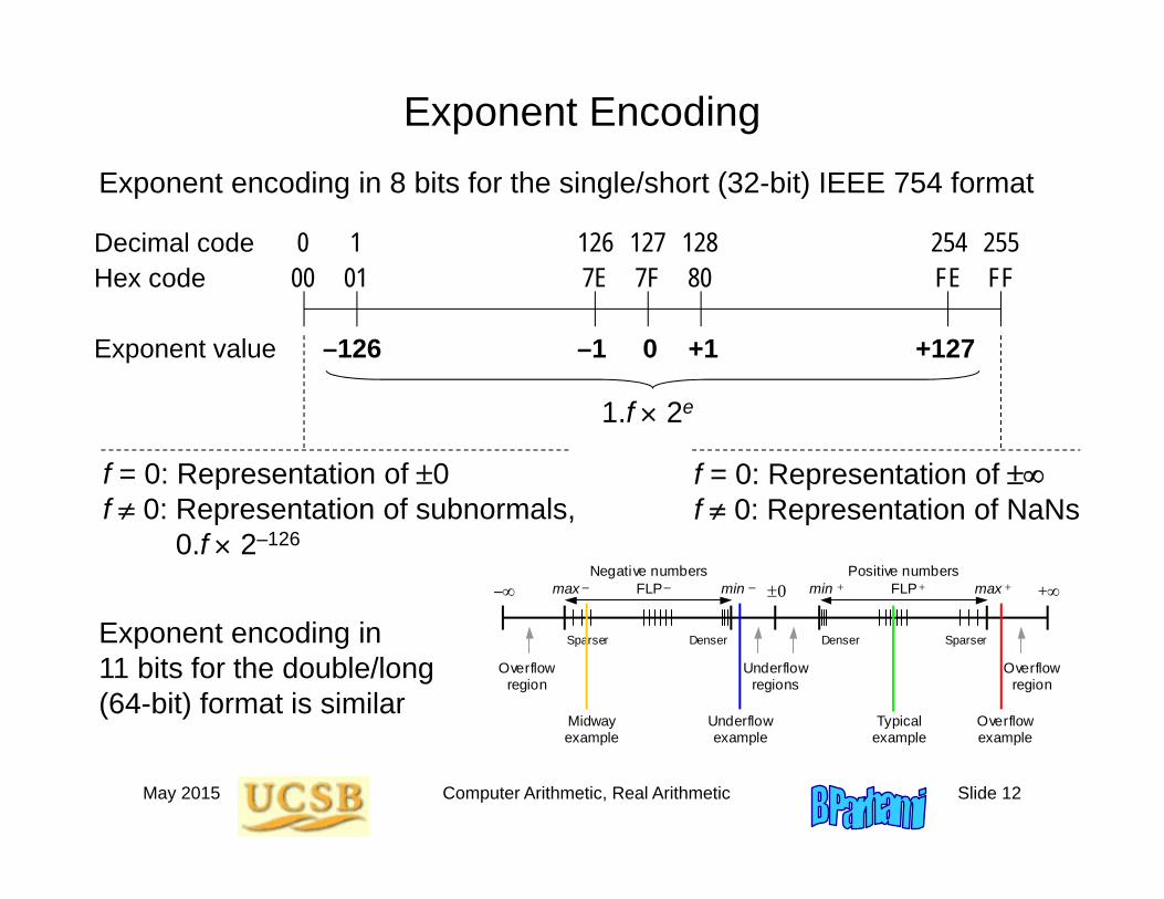
Exponent Encoding
00 01 7F FE FF7E 800 1 127 254 255126 128
–126 0 +127–1 +1
Decimal codeHex code
Exponent value
f = 0: Representation of 0f 0: Representation of subnormals,
0.f 2–126
f = 0: Representation of f 0: Representation of NaNs
Exponent encoding in 8 bits for the single/short (32-bit) IEEE 754 format
Exponent encoding in 11 bits for the double/long (64-bit) format is similar
Denser Denser Sparser Sparser
Negative numbers FLP FLP 0 +
–
Overflow region
Overflow region
Underflow regions
Positive numbers
Underflow example
Overflow example
Midway example
Typical example
min max min max + + – – – +
1.f 2e
May 2015 Computer Arithmetic, Real Arithmetic Slide 13
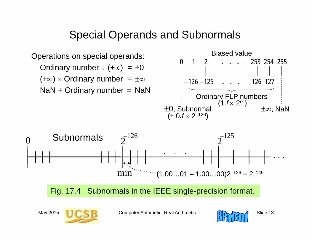
Special Operands and Subnormals
Operations on special operands:Ordinary number (+) = 0(+) Ordinary number = NaN + Ordinary number = NaN
Biased value0 1 2 . . . 253 254 255
126 125 . . . 126 127
Ordinary FLP numbers
, NaN0, Subnormal( 0.f 2–126)
(1.f 2e )
(1.00…01 – 1.00…00)2–126 = 2–149
0 2–126Denormals 2
–125
. . . . . .
min
. . .
Fig. 17.4 Subnormals in the IEEE single-precision format.
Subnormals
May 2015 Computer Arithmetic, Real Arithmetic Slide 14
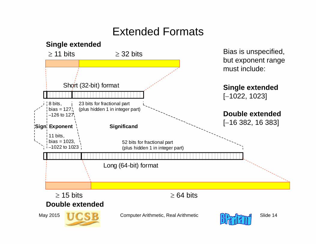
Extended Formats
Short (32-bit) format
Long (64-bit) format
Sign Exponent Significand
8 bits, bias = 127, –126 to 127
11 bits, bias = 1023, –1022 to 1023
52 bits for fractional part (plus hidden 1 in integer part)
23 bits for fractional part (plus hidden 1 in integer part)
11 bits 32 bits
15 bits 64 bits
Double extended[16 382, 16 383]
Single extended[1022, 1023]
Bias is unspecified, but exponent range must include:
Single extended
Double extended
May 2015 Computer Arithmetic, Real Arithmetic Slide 15
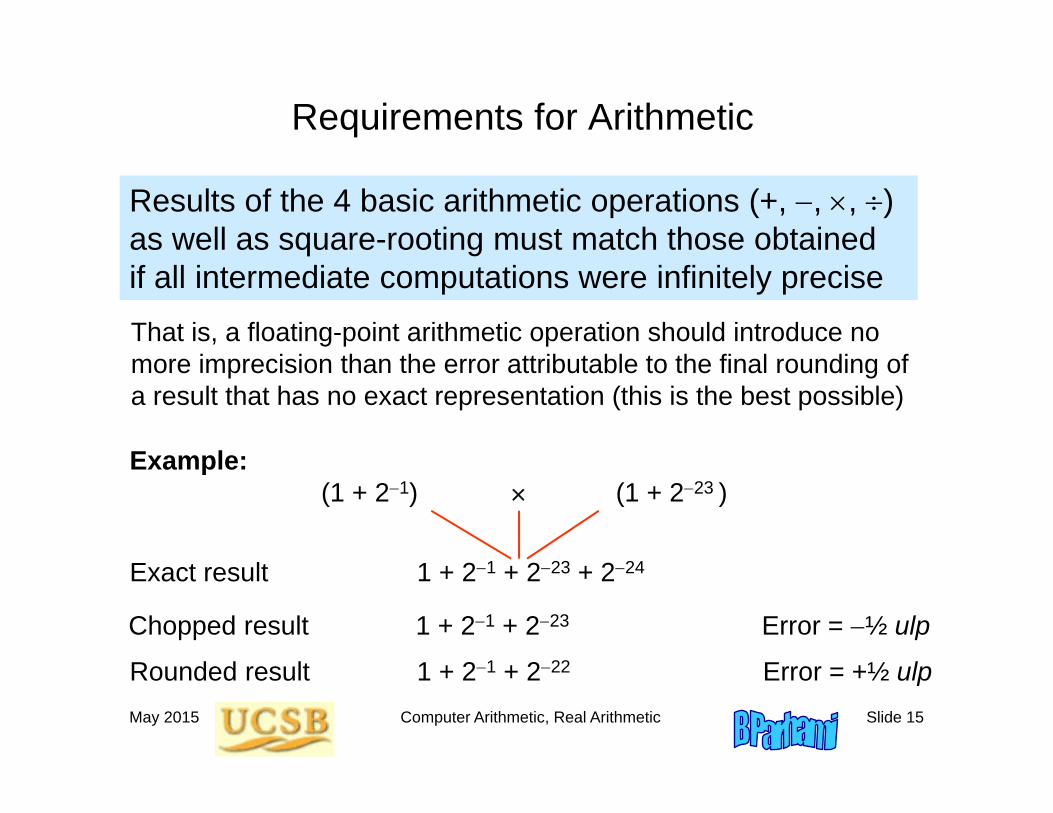
Requirements for Arithmetic
Results of the 4 basic arithmetic operations (+, , , ) as well as square-rooting must match those obtained if all intermediate computations were infinitely preciseThat is, a floating-point arithmetic operation should introduce no more imprecision than the error attributable to the final rounding of a result that has no exact representation (this is the best possible)
Example:(1 + 21) (1 + 223 )
Chopped result 1 + 21 + 223 Error = ½ ulp
Exact result 1 + 21 + 223 + 224
Rounded result 1 + 21 + 222 Error = +½ ulp
May 2015 Computer Arithmetic, Real Arithmetic Slide 16
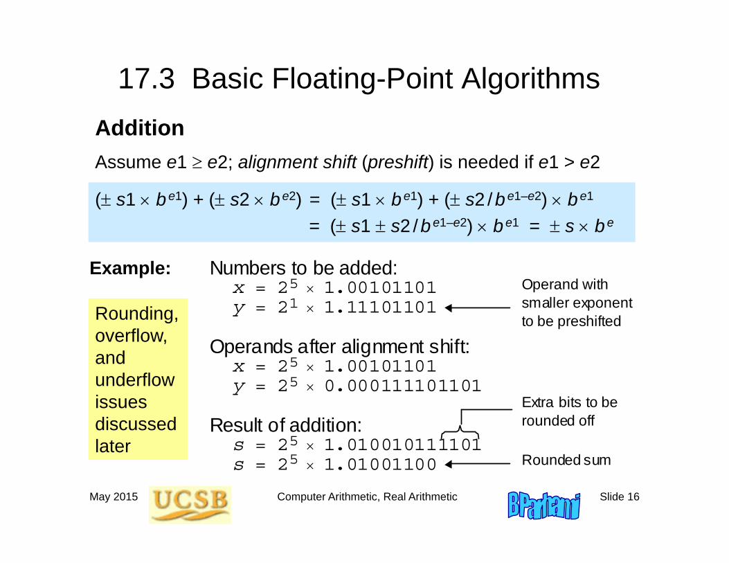
17.3 Basic Floating-Point Algorithms
( s1 be1) + ( s2 be2) = ( s1 be1) + ( s2 /be1–e2) be1
= ( s1 s2 /be1–e2) be1 = s be
Assume e1 e2; alignment shift (preshift) is needed if e1 > e2
Operands after alignment shift: x = 2 1.00101101 y = 2 0.000111101101
Numbers to be added: x = 2 1.00101101 y = 2 1.11101101
5
5
Extra bits to be rounded off
Operand with smaller exponent to be preshifted
Result of addition: s = 2 1.010010111101 s = 2 1.01001100 Rounded sum
5
1
5 5
Example:
Addition
Rounding, overflow, and underflow issues discussed later
May 2015 Computer Arithmetic, Real Arithmetic Slide 17
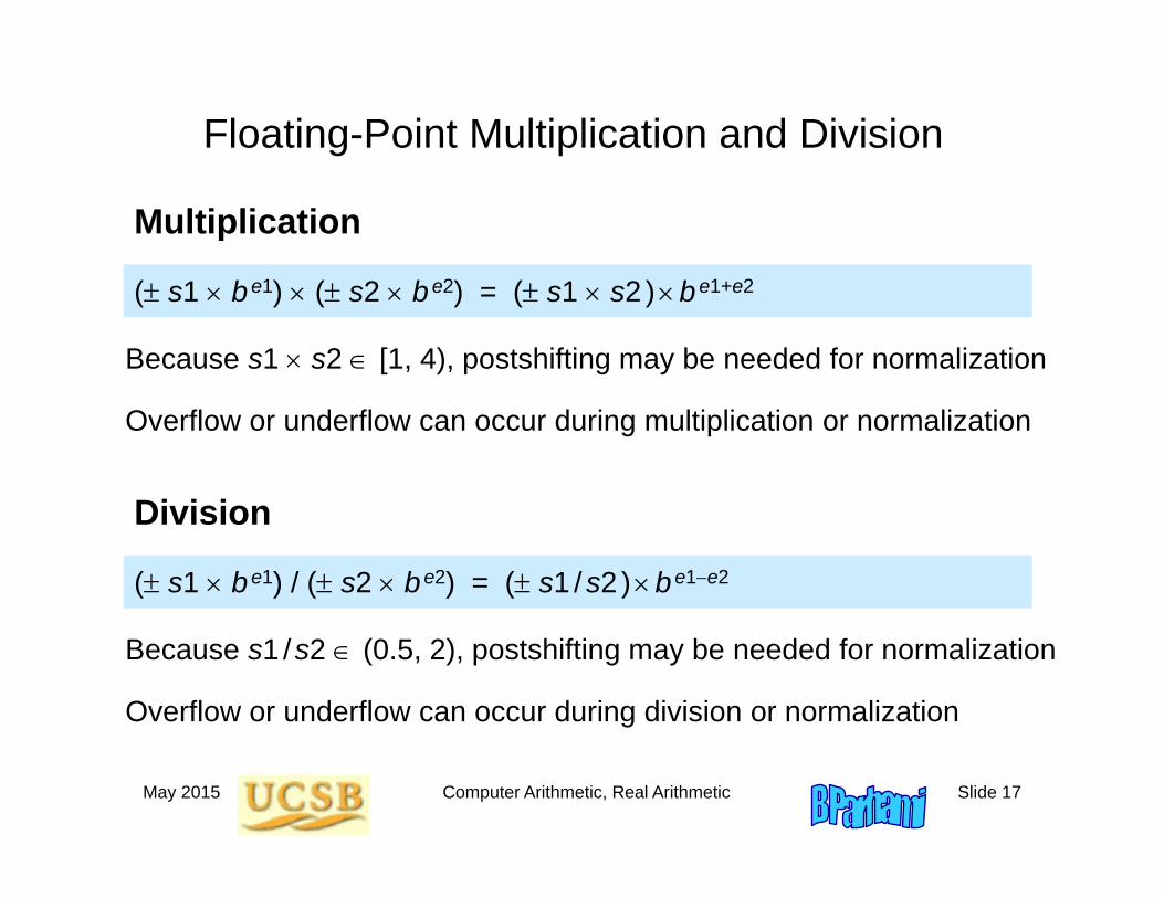
Floating-Point Multiplication and Division
Because s1 s2 [1, 4), postshifting may be needed for normalization
( s1 be1) ( s2 be2) = ( s1 s2 )be1+e2
Multiplication
Overflow or underflow can occur during multiplication or normalization
Because s1 /s2 (0.5, 2), postshifting may be needed for normalization
( s1 be1) / ( s2 be2) = ( s1 /s2 )be1e2
Division
Overflow or underflow can occur during division or normalization
May 2015 Computer Arithmetic, Real Arithmetic Slide 18
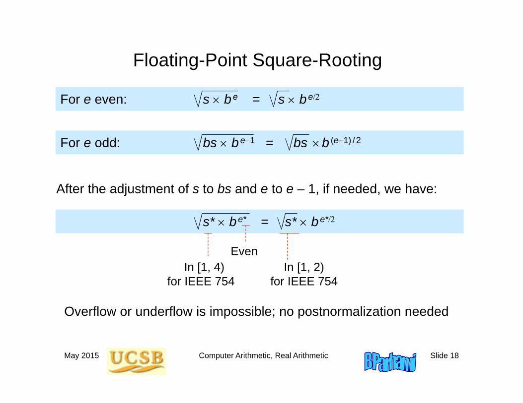
Floating-Point Square-Rooting
Overflow or underflow is impossible; no postnormalization needed
For e even: s be = s be
For e odd: bs be1 = bs b (e–1) /2
After the adjustment of s to bs and e to e – 1, if needed, we have:
s* be* = s* be*
In [1, 4)for IEEE 754
In [1, 2)for IEEE 754
Even
May 2015 Computer Arithmetic, Real Arithmetic Slide 19
17.4 Conversions and Exceptions
Conversions from fixed- to floating-pointConversions between floating-point formatsConversion from high to lower precision: Rounding
The IEEE 754-2008 standard includes five rounding modes:Round to nearest, ties away from 0 (rtna)Round to nearest, ties to even (rtne) [default rounding mode]Round toward zero (inward)Round toward + (upward)Round toward – (downward)
May 2015 Computer Arithmetic, Real Arithmetic Slide 20
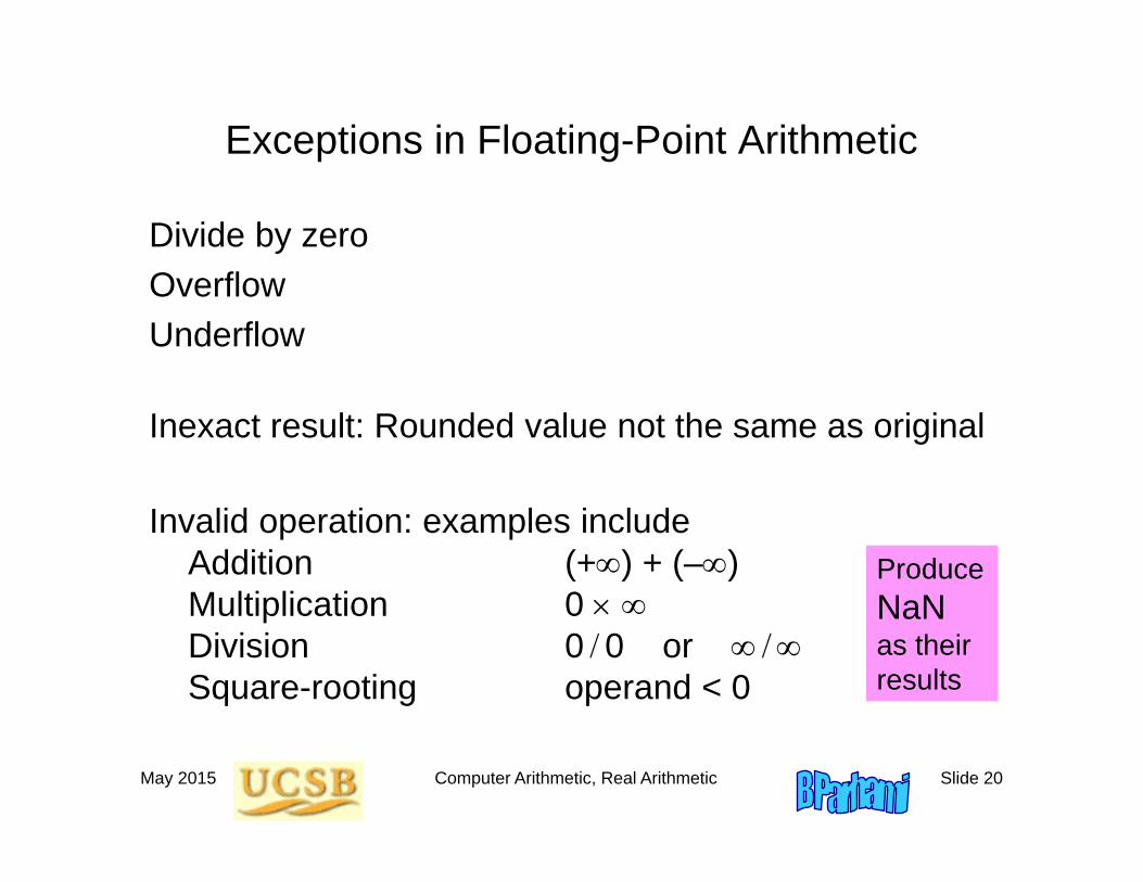
Exceptions in Floating-Point Arithmetic
Divide by zeroOverflowUnderflow
Inexact result: Rounded value not the same as original
Invalid operation: examples includeAddition (+) + (–)Multiplication 0 Division 0 0 or Square-rooting operand < 0
Produce NaNas their results
May 2015 Computer Arithmetic, Real Arithmetic Slide 21
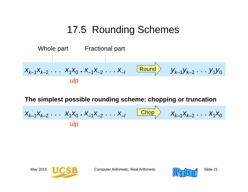
17.5 Rounding Schemes
The simplest possible rounding scheme: chopping or truncation
Fractional partWhole part
xk–1xk–2 . . . x1x0 . x–1x–2 . . . x–l yk–1yk–2 . . . y1y0Round
ulp
xk–1xk–2 . . . x1x0 . x–1x–2 . . . x–l xk–1xk–2 . . . x1x0Chop
ulp
May 2015 Computer Arithmetic, Real Arithmetic Slide 22
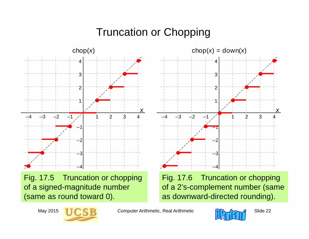
Truncation or Chopping
Fig. 17.5 Truncation or chopping of a signed-magnitude number (same as round toward 0).
chop(x)
–4
–3
–2
–1
x–4 –3 –2 –1 4 3 2 1
4
3
2
1
Fig. 17.6 Truncation or chopping of a 2’s-complement number (same as downward-directed rounding).
chop(x) = down(x)
–4
–3
–2
–1
x–4 –3 –2 –1 4 3 2 1
4
3
2
1
May 2015 Computer Arithmetic, Real Arithmetic Slide 23
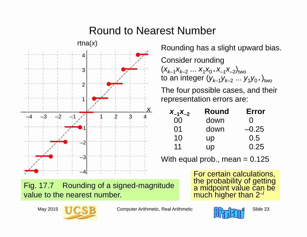
Round to Nearest Number
Fig. 17.7 Rounding of a signed-magnitude value to the nearest number.
Rounding has a slight upward bias.Consider rounding (xk–1xk–2 ... x1x0 .x–1x–2)twoto an integer (yk–1yk–2 ... y1y0 . )two
The four possible cases, and their representation errors are:
x–1x–2 Round Error00 down 001 down –0.2510 up 0.511 up 0.25
With equal prob., mean = 0.125
For certain calculations, the probability of getting a midpoint value can be much higher than 2–l
rtn(x)
–4
–3
–2
–1
x–4 –3 –2 –1 4 3 2 1
4
3
2
1
rtna(x)
May 2015 Computer Arithmetic, Real Arithmetic Slide 24
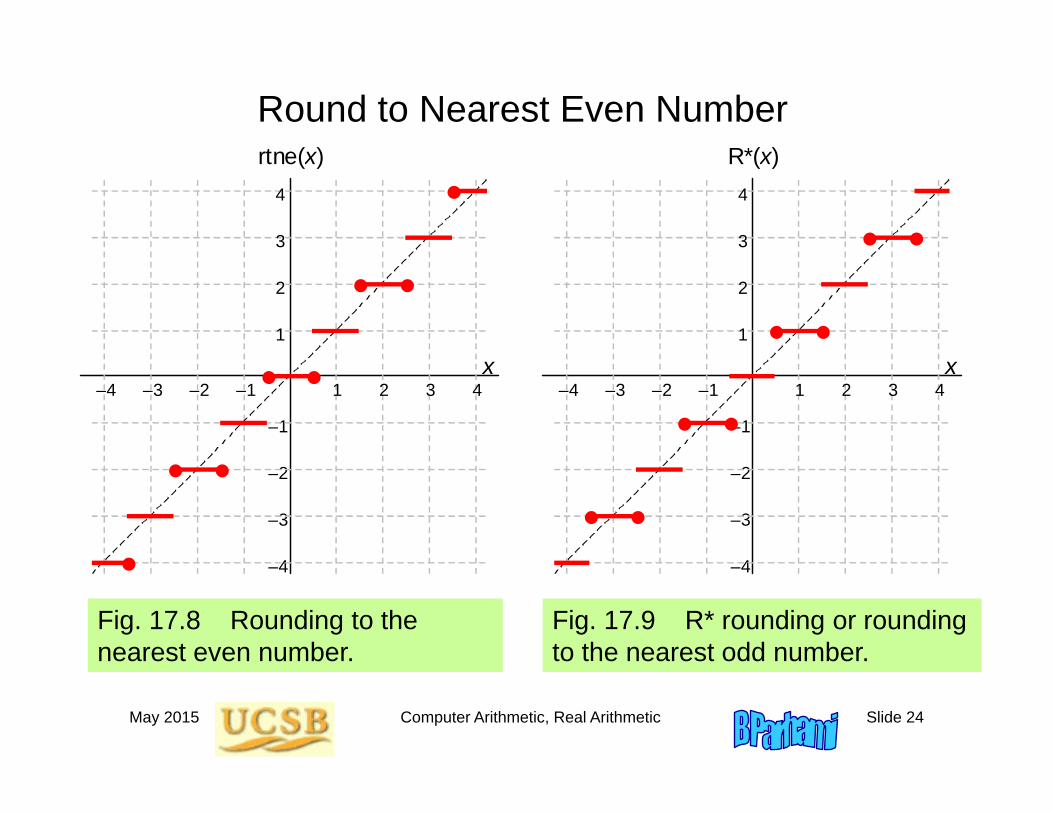
Round to Nearest Even Number
Fig. 17.8 Rounding to the nearest even number.
rtne(x)
–4
–3
–2
–1
x–4 –3 –2 –1 4 3 2 1
4
3
2
1
Fig. 17.9 R* rounding or rounding to the nearest odd number.
R*(x)
–4
–3
–2
–1
x–4 –3 –2 –1 4 3 2 1
4
3
2
1
May 2015 Computer Arithmetic, Real Arithmetic Slide 25
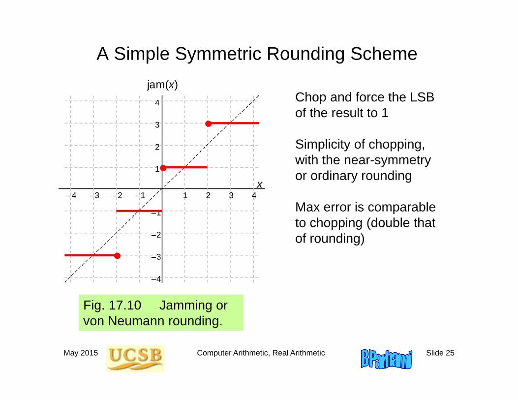
A Simple Symmetric Rounding Scheme
Fig. 17.10 Jamming or von Neumann rounding.
jam(x)
–4
–3
–2
–1
x–4 –3 –2 –1 4 3 2 1
4
3
2
1
Chop and force the LSB of the result to 1
Simplicity of chopping, with the near-symmetry or ordinary rounding
Max error is comparable to chopping (double that of rounding)

May 2015 Computer Arithmetic, Real Arithmetic Slide 26
ROM RoundingFig. 17.11 ROM rounding with an 8 2 table.
Example: Rounding with a 32 4 table
ROM(x)
–4
–3
–2
–1
x–4 –3 –2 –1 4 3 2 1
4
3
2
1
Rounding result is the same as that of the round to nearest scheme in 31 of the 32 possible cases, but a larger error is introduced when
x3 = x2 = x1 = x0 = x–1 = 1
xk–1 . . . x4x3x2x1x0 . x–1x–2 . . . x–l xk–1 . . . x4y3y2y1y0ROMROM dataROM address
May 2015 Computer Arithmetic, Real Arithmetic Slide 27
Directed Rounding: Motivation
We may need result errors to be in a known direction
Example: in computing upper bounds, larger results are acceptable, but results that are smaller than correct values could invalidate the upper bound
This leads to the definition of directed rounding modesupward-directed rounding (round toward +) and downward-directed rounding (round toward –)(required features of IEEE floating-point standard)
May 2015 Computer Arithmetic, Real Arithmetic Slide 28
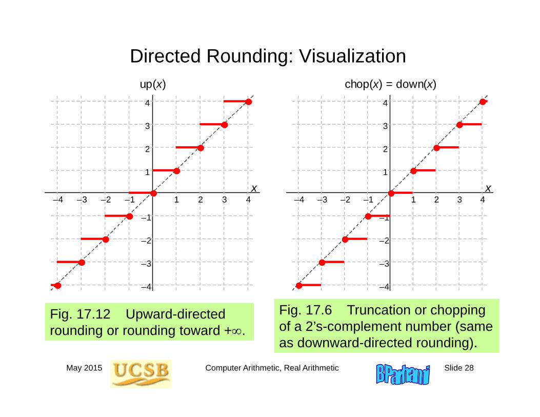
Directed Rounding: Visualization
Fig. 17.12 Upward-directed rounding or rounding toward +.
Fig. 17.6 Truncation or chopping of a 2’s-complement number (same as downward-directed rounding).
up(x)
–4
–3
–2
–1
x–4 –3 –2 –1 4 3 2 1
4
3
2
1
chop(x) = down(x)
–4
–3
–2
–1
x–4 –3 –2 –1 4 3 2 1
4
3
2
1
May 2015 Computer Arithmetic, Real Arithmetic Slide 29
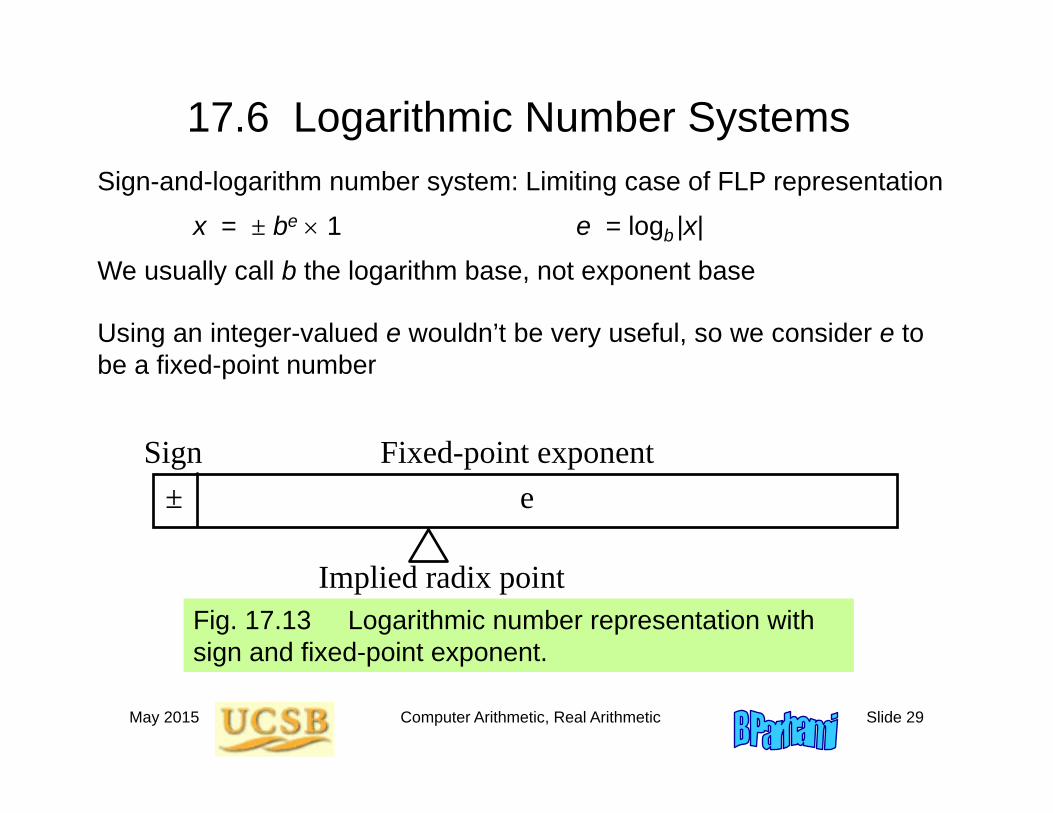
17.6 Logarithmic Number SystemsSign-and-logarithm number system: Limiting case of FLP representation
x = ± be 1 e = logb |x|
We usually call b the logarithm base, not exponent base
Using an integer-valued e wouldn’t be very useful, so we consider e tobe a fixed-point number
Sign
Implied radix point
e±Fixed-point exponent
Fig. 17.13 Logarithmic number representation with sign and fixed-point exponent.
May 2015 Computer Arithmetic, Real Arithmetic Slide 30
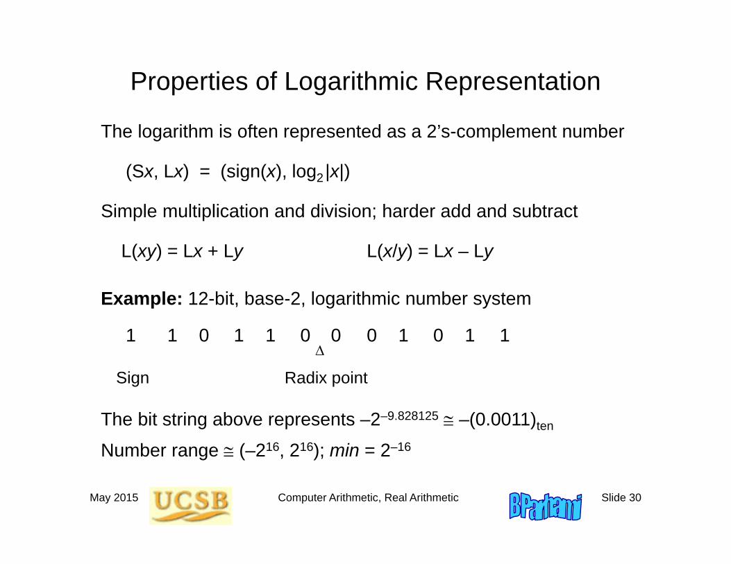
Properties of Logarithmic Representation
The logarithm is often represented as a 2’s-complement number
(Sx, Lx) = (sign(x), log2|x|)
Simple multiplication and division; harder add and subtract
L(xy) = Lx + Ly L(x/y) = Lx – Ly
Example: 12-bit, base-2, logarithmic number system
1 1 0 1 1 0 0 0 1 0 1 1
Sign Radix point
The bit string above represents –2–9.828125 –(0.0011)ten
Number range (–216, 216); min = 2–16
May 2015 Computer Arithmetic, Real Arithmetic Slide 31
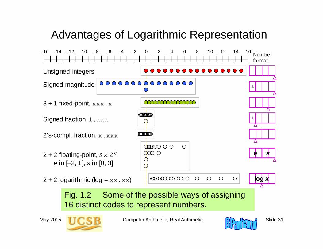
Advantages of Logarithmic Representation
Fig. 1.2 Some of the possible ways of assigning 16 distinct codes to represent numbers.
0 2 4 6 8 10 12 14 16 2 4 6 8 10 12 14 16
Unsigned integers
Signed-magnitude
3 + 1 fixed-point, xxx.x
Signed fraction, .xxx
2’s-compl. fraction, x.xxx
2 + 2 floating-point, s 2 e in [2, 1], s in [0, 3]
2 + 2 logarithmic (log = xx.xx)
Number format
log x
s e e
May 2015 Computer Arithmetic, Real Arithmetic Slide 32
18 Floating-Point Operations
Chapter GoalsSee how adders, multipliers, and dividersare designed for floating-point operands(square-rooting postponed to Chapter 21)
Chapter HighlightsFloating-point operation = preprocessing +
exponent and significand arithmetic +postprocessing (+ exception handling)
Adders need preshift, postshift, roundingMultipliers and dividers are easy to design
May 2015 Computer Arithmetic, Real Arithmetic Slide 33
Floating-Point Operations: Topics
Topics in This Chapter
18.1 Floating-Point Adders /Subtractors
18.2 Pre- and Postshifting
18.3 Rounding and Exceptions
18.4 Floating-Point Multipliers and Dividers
18.5 Fused-Multiply-Add Units
18.6 Logarithmic Arithmetic Units
May 2015 Computer Arithmetic, Real Arithmetic Slide 34
18.1 Floating-Point Adders/Subtractors
-
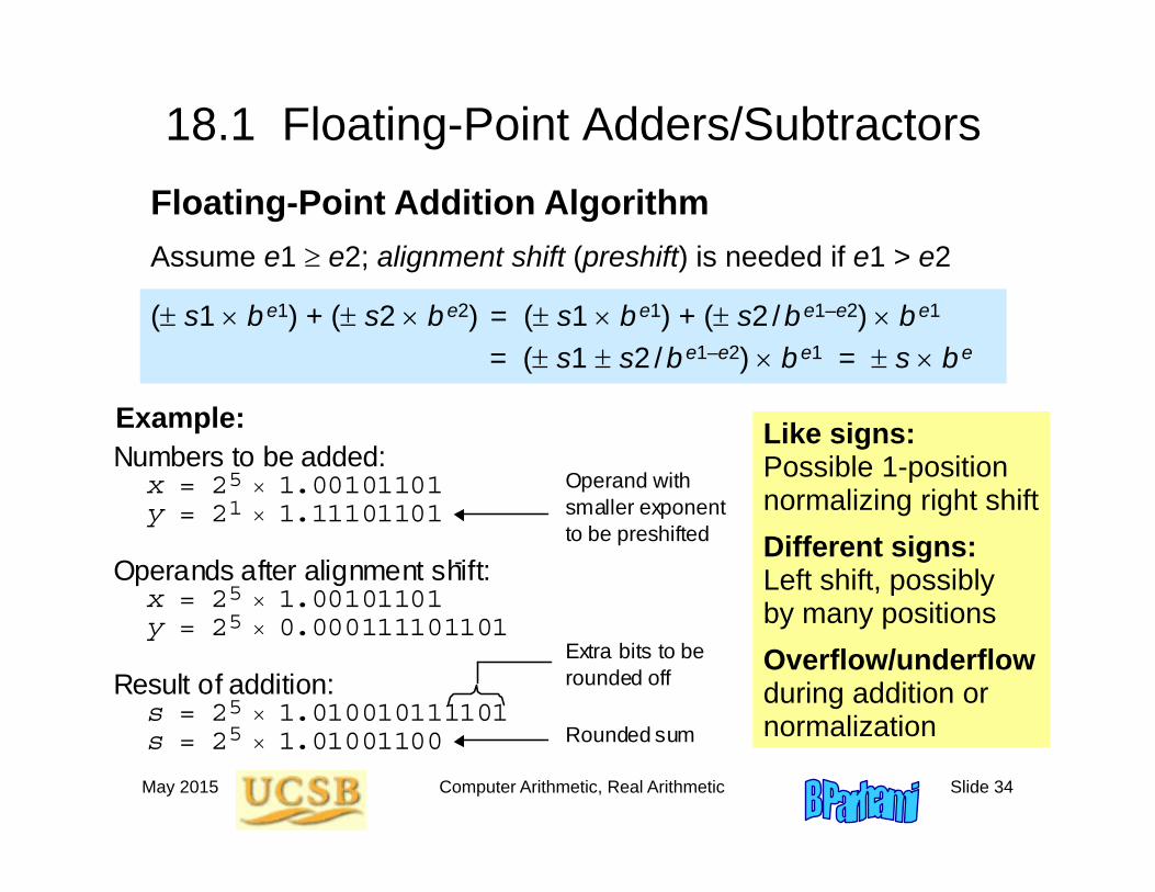
( s1 be1) + ( s2 be2) = ( s1 be1) + ( s2 /be1–e2) be1
= ( s1 s2 /be1–e2) be1 = s be
Assume e1 e2; alignment shift (preshift) is needed if e1 > e2
Operands after alignment shift: x = 2 1.00101101 y = 2 0.000111101101
Numbers to be added: x = 2 1.00101101 y = 2 1.11101101
5
5
Extra bits to be rounded off
Operand with smaller exponent to be preshifted
Result of addition: s = 2 1.010010111101 s = 2 1.01001100 Rounded sum
5
1
5 5
Example:
Floating-Point Addition Algorithm
Like signs:Possible 1-position normalizing right shiftDifferent signs:Left shift, possibly by many positionsOverflow/underflowduring addition or normalization
May 2015 Computer Arithmetic, Real Arithmetic Slide 35
FLP Addition Hardware
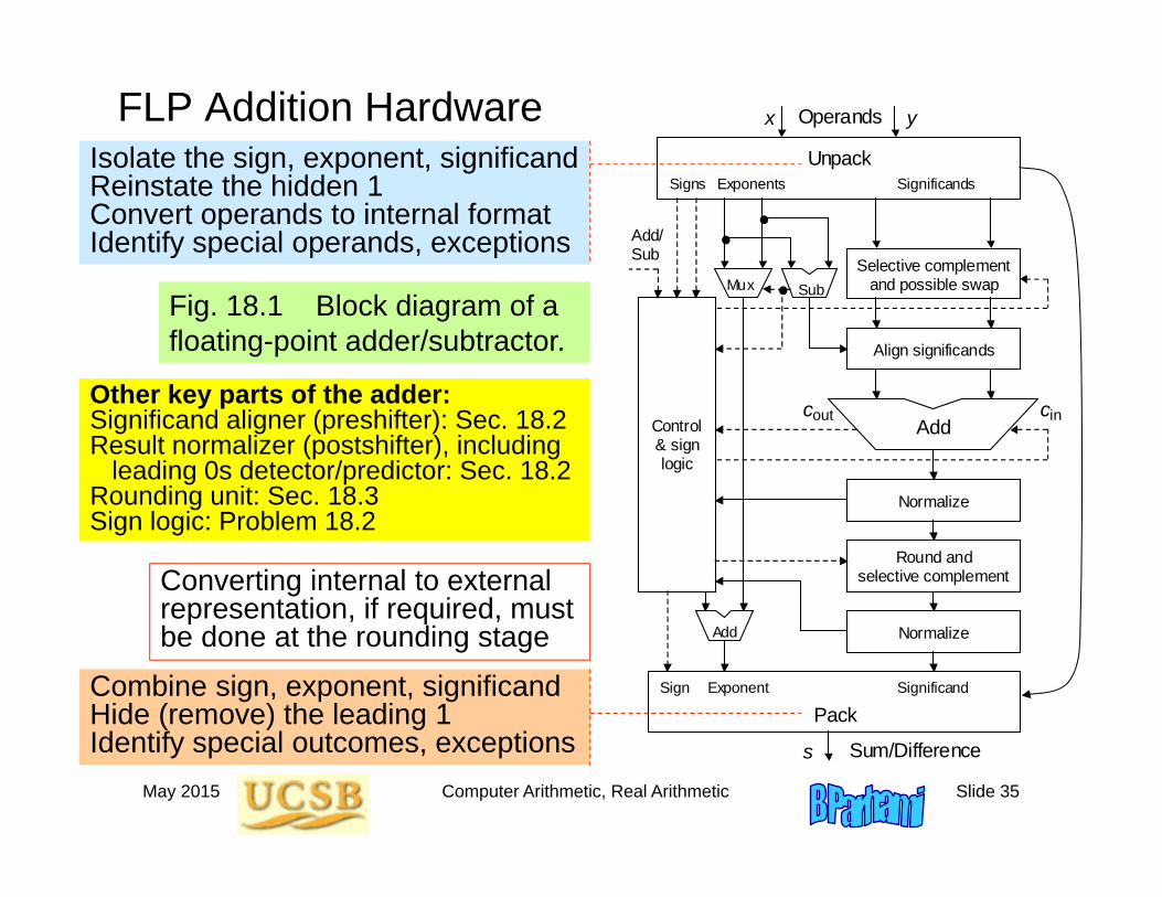
Fig. 18.1 Block diagram of a floating-point adder/subtractor.
Normalize
Add
Align significands
Unpack
Control & sign logic
Add/ Sub
Pack
Operands
Sum/Difference
Significands Exponents Signs
Significand Exponent Sign
x y
s
Sub
Add
Mux
c out c in
Selective complement and possible swap
Round and selective complement
Normalize
Other key parts of the adder:Significand aligner (preshifter): Sec. 18.2Result normalizer (postshifter), including
leading 0s detector/predictor: Sec. 18.2Rounding unit: Sec. 18.3Sign logic: Problem 18.2
Converting internal to external representation, if required, must be done at the rounding stage
Isolate the sign, exponent, significandReinstate the hidden 1Convert operands to internal formatIdentify special operands, exceptions
Combine sign, exponent, significandHide (remove) the leading 1Identify special outcomes, exceptions
May 2015 Computer Arithmetic, Real Arithmetic Slide 36
Types of Post-Normalization
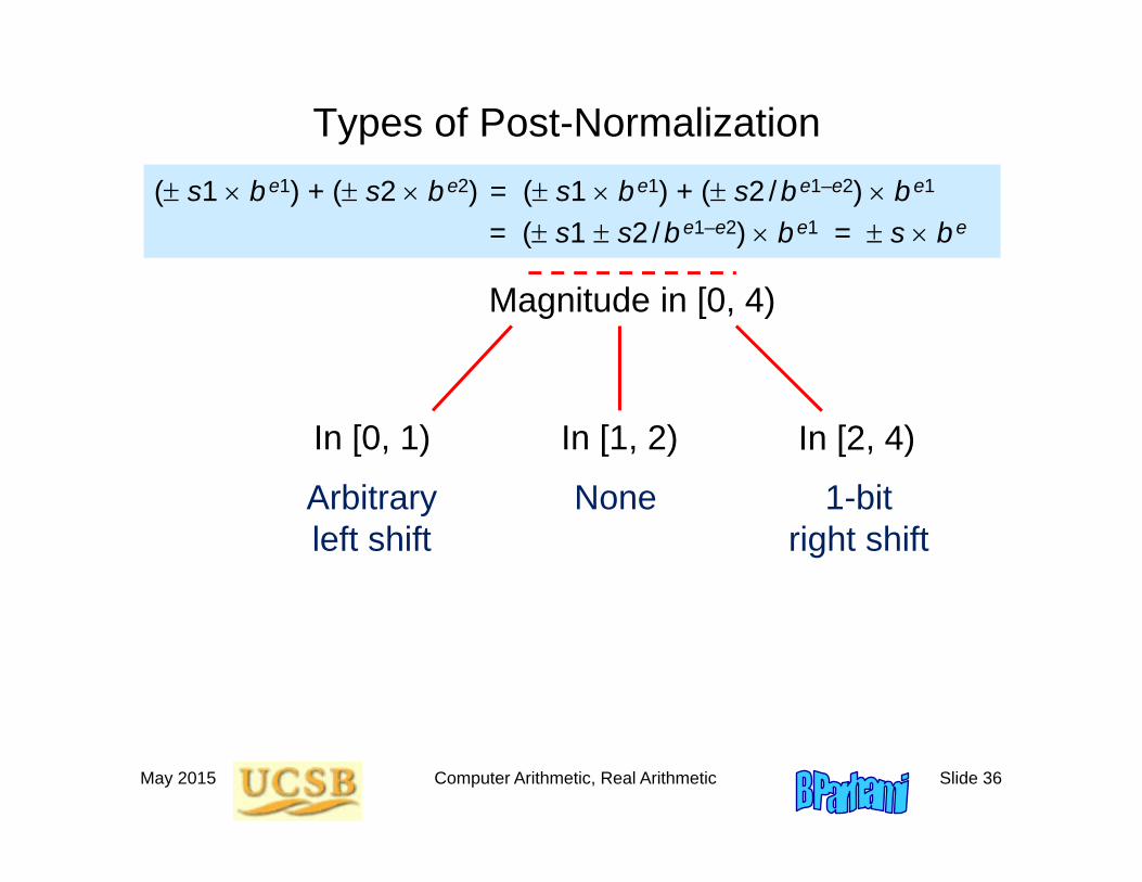
Magnitude in [0, 4)
( s1 be1) + ( s2 be2) = ( s1 be1) + ( s2 /be1–e2) be1
= ( s1 s2 /be1–e2) be1 = s be
In [0, 1) In [1, 2) In [2, 4)
None 1-bitright shift
Arbitraryleft shift
May 2015 Computer Arithmetic, Real Arithmetic Slide 37
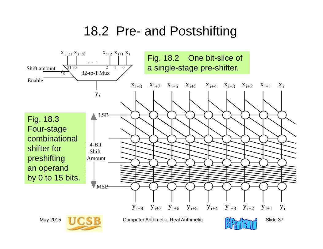
18.2 Pre- and Postshifting
Fig. 18.2 One bit-slice of a single-stage pre-shifter.
xixi+2 xi+1xi+4 xi+3xi+6 xi+5xi+8 xi+7
yiyi+2 yi+1yi+4 yi+3yi+6 yi+5yi+8 yi+7
LSB
MSB
4-Bit Shift Amount
y i
x ix i+2 x i+1x i+30x i+31
5Shift amount 31 30 2 1 0
. . .
32-to-1 MuxEnable
Fig. 18.3 Four-stage combinational shifter for preshifting an operand by 0 to 15 bits.
May 2015 Computer Arithmetic, Real Arithmetic Slide 38
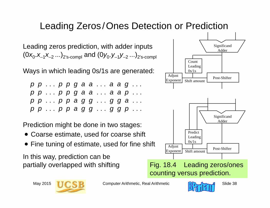
Leading Zeros /Ones Detection or Prediction
Leading zeros prediction, with adder inputs(0x0.x–1x–2 ...)2’s-compl and (0y0.y–1y–2 ...)2’s-compl
Ways in which leading 0s/1s are generated:
p p . . . p p g a a . . . a a g . . .p p . . . p p g a a . . . a a p . . .p p . . . p p a g g . . . g g a . . .p p . . . p p a g g . . . g g p . . .
Prediction might be done in two stages: Coarse estimate, used for coarse shift Fine tuning of estimate, used for fine shift
In this way, prediction can be partially overlapped with shifting
Shift amountPost-Shifter
Significand Adder
Adjust Exponent
Count Leading 0s/1s
Post-Shifter
Significand Adder
Adjust Exponent
Predict Leading 0s/1s
Shift amount
Fig. 18.4 Leading zeros/ones counting versus prediction.
May 2015 Computer Arithmetic, Real Arithmetic Slide 39
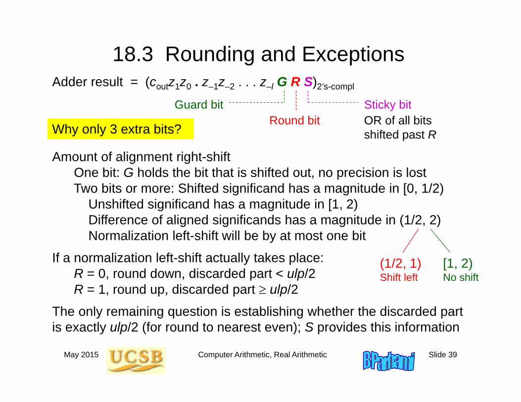
18.3 Rounding and Exceptions
Amount of alignment right-shift One bit: G holds the bit that is shifted out, no precision is lost Two bits or more: Shifted significand has a magnitude in [0, 1/2)
Unshifted significand has a magnitude in [1, 2)Difference of aligned significands has a magnitude in (1/2, 2)Normalization left-shift will be by at most one bit
If a normalization left-shift actually takes place:R = 0, round down, discarded part < ulp/2R = 1, round up, discarded part ulp/2
The only remaining question is establishing whether the discarded part is exactly ulp/2 (for round to nearest even); S provides this information
Round bit
Adder result = (coutz1z0 . z–1z–2 . . . z–l G R S)2’s-compl
Sticky bitGuard bitOR of all bits shifted past RWhy only 3 extra bits?
(1/2, 1)Shift left
[1, 2)No shift
May 2015 Computer Arithmetic, Real Arithmetic Slide 40
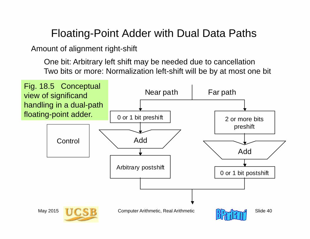
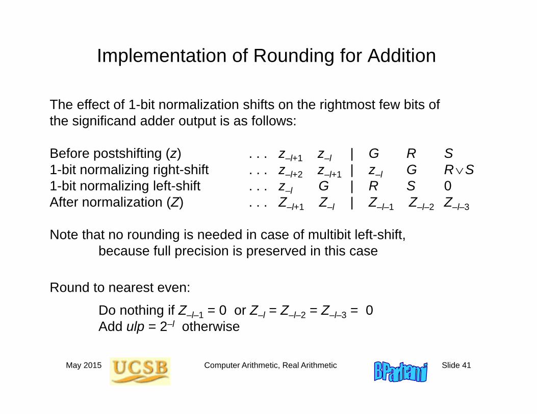
Floating-Point Adder with Dual Data Paths
Near path Far path
0 or 1 bit preshift Arbitrary preshift
0 or 1 bit postshift Arbitrary postshift
Add Add
Control
Amount of alignment right-shift
One bit: Arbitrary left shift may be needed due to cancellation Two bits or more: Normalization left-shift will be by at most one bit
Fig. 18.5 Conceptual view of significand handling in a dual-path floating-point adder.
2 or more bits preshift
May 2015 Computer Arithmetic, Real Arithmetic Slide 41
Implementation of Rounding for Addition
Round to nearest even:
Do nothing if Z–l–1 = 0 or Z–l = Z–l–2 = Z–l–3 = 0 Add ulp = 2–l otherwise
The effect of 1-bit normalization shifts on the rightmost few bits of the significand adder output is as follows:
Before postshifting (z) . . . z–l+1 z–l | G R S1-bit normalizing right-shift . . . z–l+2 z–l+1 | z–l G RS1-bit normalizing left-shift . . . z–l G | R S 0After normalization (Z) . . . Z–l+1 Z–l | Z–l–1 Z–l–2 Z–l–3
Note that no rounding is needed in case of multibit left-shift, because full precision is preserved in this case
May 2015 Computer Arithmetic, Real Arithmetic Slide 42
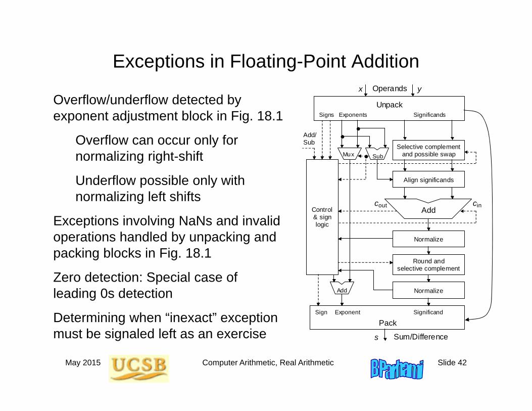
Exceptions in Floating-Point Addition
Overflow/underflow detected by exponent adjustment block in Fig. 18.1
Overflow can occur only for normalizing right-shift
Underflow possible only with normalizing left shifts
Exceptions involving NaNs and invalid operations handled by unpacking and packing blocks in Fig. 18.1
Zero detection: Special case of leading 0s detection
Determining when “inexact” exception must be signaled left as an exercise
Normalize
Add
Align significands
Unpack
Control & sign logic
Add/ Sub
Pack
Operands
Sum/Difference
Significands Exponents Signs
Significand Exponent Sign
x y
s
Sub
Add
Mux
c out c in
Selective complement and possible swap
Round and selective complement
Normalize
May 2015 Computer Arithmetic, Real Arithmetic Slide 43
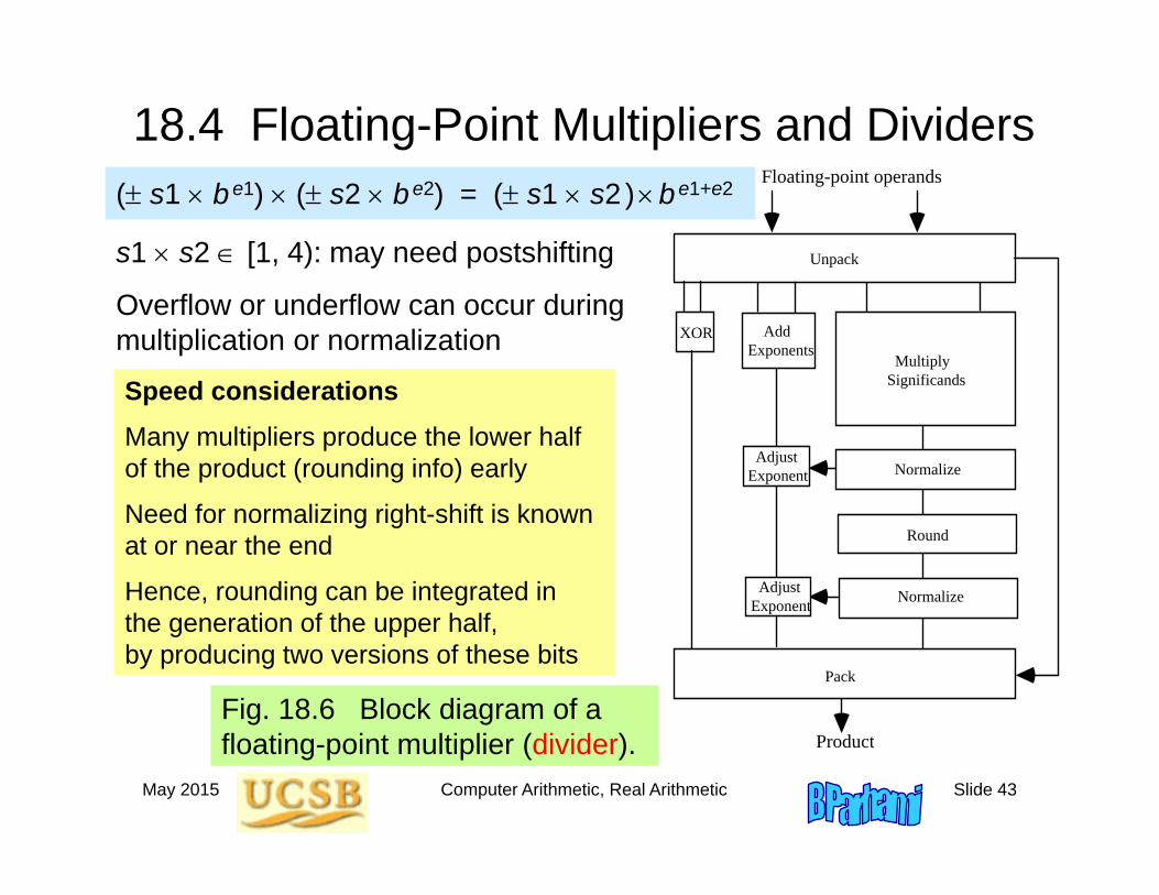
18.4 Floating-Point Multipliers and Dividers
Fig. 18.6 Block diagram of a floating-point multiplier (divider).
Speed considerationsMany multipliers produce the lower half of the product (rounding info) early
Need for normalizing right-shift is known at or near the end
Hence, rounding can be integrated in the generation of the upper half, by producing two versions of these bits
s1 s2 [1, 4): may need postshifting
( s1 be1) ( s2 be2) = ( s1 s2 )be1+e2
XOR Add Exponents
Unpack
Normalize Adjust Exponent
Round
Normalize
Pack
Multiply Significands
Floating-point operands
Product
Adjust Exponent
Overflow or underflow can occur during multiplication or normalization
May 2015 Computer Arithmetic, Real Arithmetic Slide 44
XOR Subtract Exponents
Unpack
Normalize Adjust Exponent
Round
Normalize
Pack
Divide Significands
Floating-point operands
Quotient
Adjust Exponent
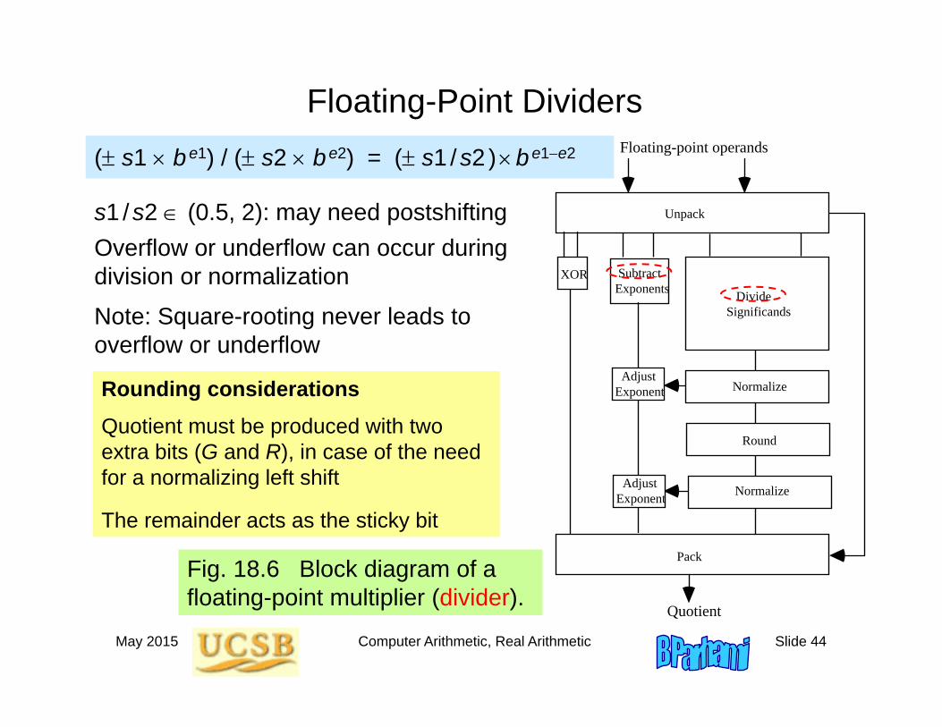
Floating-Point Dividers
Rounding considerationsQuotient must be produced with two extra bits (G and R), in case of the need for a normalizing left shift
The remainder acts as the sticky bit
s1 /s2 (0.5, 2): may need postshifting
( s1 be1) / ( s2 be2) = ( s1 /s2 )be1e2
Overflow or underflow can occur during division or normalization
Note: Square-rooting never leads to overflow or underflow
Fig. 18.6 Block diagram of a floating-point multiplier (divider).
May 2015 Computer Arithmetic, Real Arithmetic Slide 45
18.5 Fused-Multiply-Add Units
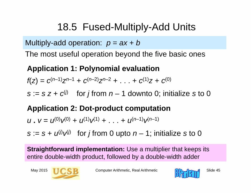
Application 1: Polynomial evaluationf(z) = c(n–1)zn–1 + c(n–2)zn–2 + . . . + c(1)z + c(0)
s := s z + c(j) for j from n – 1 downto 0; initialize s to 0
Multiply-add operation: p = ax + bThe most useful operation beyond the five basic ones
Application 2: Dot-product computationu . v = u(0)v(0) + u(1)v(1) + . . . + u(n–1)v(n–1)
s := s + u(j)v(j) for j from 0 upto n – 1; initialize s to 0
Straightforward implementation: Use a multiplier that keeps its entire double-width product, followed by a double-width adder
May 2015 Computer Arithmetic, Real Arithmetic Slide 46
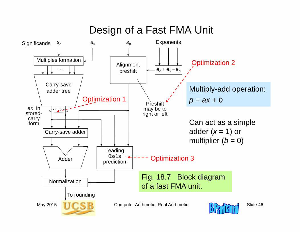
Design of a Fast FMA Unit
Fig. 18.7 Block diagram of a fast FMA unit.
Can act as a simple adder (x = 1) or multiplier (b = 0)
Multiply-add operation: p = ax + b
. . .
Exponentssa
Alignment preshift
ax in stored-carry form
Carry-save adder tree
Multiples formation
Adder
Normalization
To rounding
Leading 0s/1s
prediction
ea + ex – eb
Preshift may be to right or left
Carry-save adder
sx sbSignificands
Optimization 1
Optimization 2
Optimization 3
May 2015 Computer Arithmetic, Real Arithmetic Slide 47
18.6 Logarithmic Arithmetic Unit
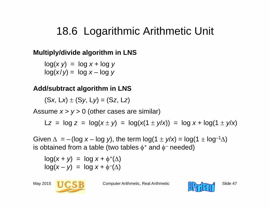
Multiply/divide algorithm in LNSlog(x y) = log x + log ylog(x /y) = log x – log y
Add/subtract algorithm in LNS(Sx, Lx) (Sy, Ly) = (Sz, Lz)
Assume x > y > 0 (other cases are similar)
Lz = log z = log(x y) = log(x(1 y/x)) = log x + log(1 y/x)
Given = – (log x – log y), the term log(1 y/x) = log(1 ± log–1)is obtained from a table (two tables + and – needed)
log(x + y) = log x + +() log(x – y) = log x + –()
May 2015 Computer Arithmetic, Real Arithmetic Slide 48
Four-Function Logarithmic Arithmetic Unit
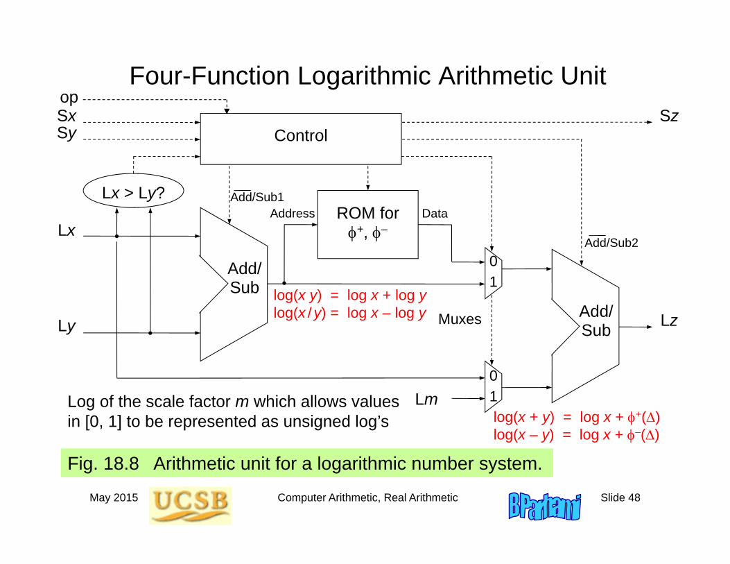
Fig. 18.8 Arithmetic unit for a logarithmic number system.
log(x + y) = log x + +() log(x – y) = log x + –()
log(x y) = log x + log ylog(x / y) = log x – log y
Log of the scale factor m which allows values in [0, 1] to be represented as unsigned log’s
Add/ Sub
Lx > Ly?
Add/ Sub
ROM for +, –
Lm
Lx
Ly
SxSy
Lz
Sz
Muxes
01
01
Control
Add/Sub1
Add/Sub2
Address Data
op
May 2015 Computer Arithmetic, Real Arithmetic Slide 49
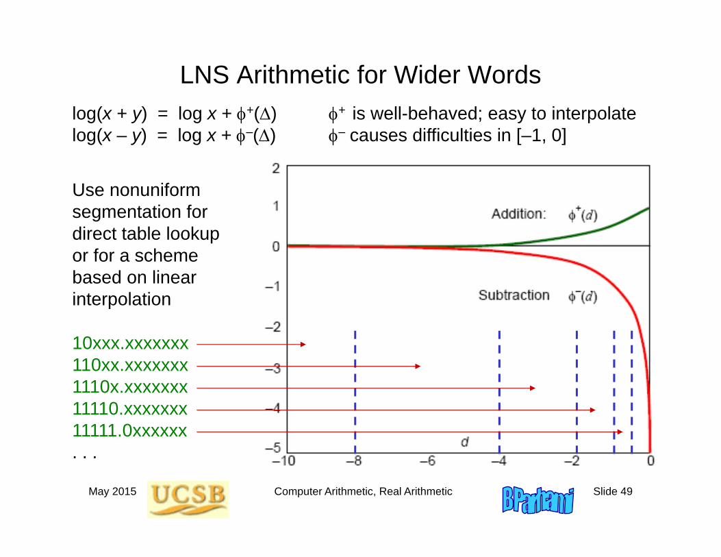
LNS Arithmetic for Wider Wordslog(x + y) = log x + +() log(x – y) = log x + –()
+ is well-behaved; easy to interpolate – causes difficulties in [–1, 0]
Use nonuniform segmentation for direct table lookup or for a scheme based on linear interpolation
10xxx.xxxxxxx110xx.xxxxxxx1110x.xxxxxxx11110.xxxxxxx11111.0xxxxxx. . .
May 2015 Computer Arithmetic, Real Arithmetic Slide 50
19 Errors and Error Control
Chapter GoalsLearn about sources of computation errors,consequences of inexact arithmetic,and methods for avoiding or limiting errors
Chapter HighlightsRepresentation and computation errorsAbsolute versus relative errorWorst-case versus average errorWhy 3 (1/3) does not necessarily yield 1Error analysis and bounding
May 2015 Computer Arithmetic, Real Arithmetic Slide 51
Errors and Error Control: Topics
Topics in This Chapter
19.1 Sources of Computational Errors
19.2 Invalidated Laws of Algebra
19.3 Worst-Case Error Accumulation
19.4 Error Distribution and Expected Errors
19.5 Forward Error Analysis
19.6 Backward Error Analysis
May 2015 Computer Arithmetic, Real Arithmetic Slide 52
19.1 Sources of Computational Errors
FLP approximates exact computation with real numbers
Two sources of errors to understand and counteract:
Representation errors
e.g., no machine representation for 1/3, 2, or
Arithmetic errors
e.g., (1 + 2–12)2 = 1 + 2–11 + 2–24
not representable in IEEE 754 short format
We saw early in the course that errors due to finite precision can lead to disasters in life-critical applications
May 2015 Computer Arithmetic, Real Arithmetic Slide 53
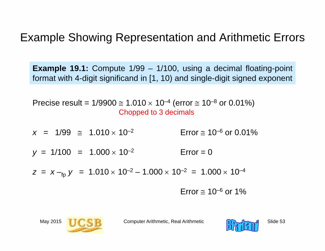
Example Showing Representation and Arithmetic Errors
Precise result = 1/9900 1.010 10–4 (error 10–8 or 0.01%)
Example 19.1: Compute 1/99 – 1/100, using a decimal floating-pointformat with 4-digit significand in [1, 10) and single-digit signed exponent
x = 1/99 1.010 10–2 Error 10–6 or 0.01%
y = 1/100 = 1.000 10–2 Error = 0
z = x –fp y = 1.010 10–2 – 1.000 10–2 = 1.000 10–4
Error 10–6 or 1%
Chopped to 3 decimals
May 2015 Computer Arithmetic, Real Arithmetic Slide 54
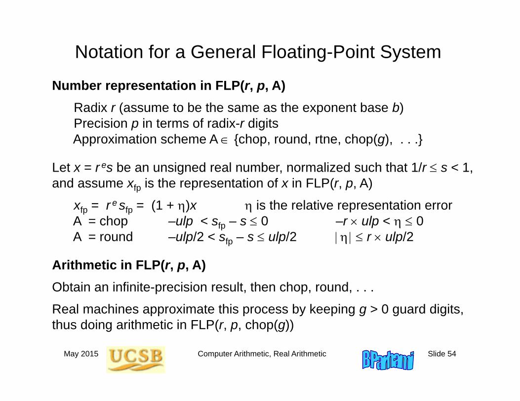
Notation for a General Floating-Point System
Number representation in FLP(r, p, A)Radix r (assume to be the same as the exponent base b)Precision p in terms of radix-r digitsApproximation scheme A {chop, round, rtne, chop(g), . . .}
Let x = r es be an unsigned real number, normalized such that 1/r s < 1, and assume xfp is the representation of x in FLP(r, p, A)
xfp = r e sfp = (1 + )x is the relative representation errorA = chop –ulp < sfp – s 0 –r ulp < 0 A = round –ulp/2 < sfp – s ulp/2 r ulp/2
Arithmetic in FLP(r, p, A) Obtain an infinite-precision result, then chop, round, . . .
Real machines approximate this process by keeping g > 0 guard digits, thus doing arithmetic in FLP(r, p, chop(g))
May 2015 Computer Arithmetic, Real Arithmetic Slide 55
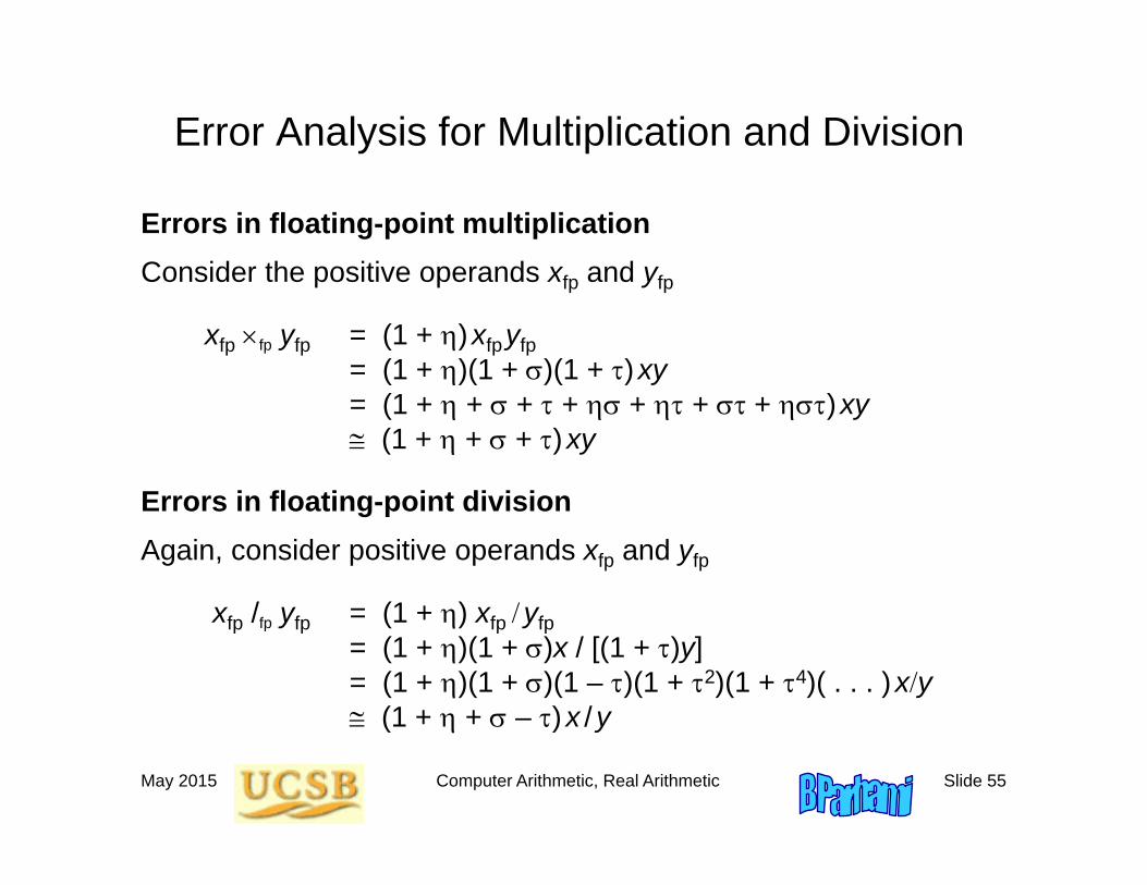
Error Analysis for Multiplication and Division
Errors in floating-point divisionAgain, consider positive operands xfp and yfp
xfp /fp yfp = (1 + ) xfp yfp= (1 + )(1 + )x / [(1 + )y]= (1 + )(1 + )(1 – )(1 + 2)(1 + 4)( . . . )xy (1 + + – )x /y
Errors in floating-point multiplicationConsider the positive operands xfp and yfp
xfp fp yfp = (1 + )xfpyfp= (1 + )(1 + )(1 + )xy= (1 + + + + + + + )xy (1 + + + )xy
May 2015 Computer Arithmetic, Real Arithmetic Slide 56
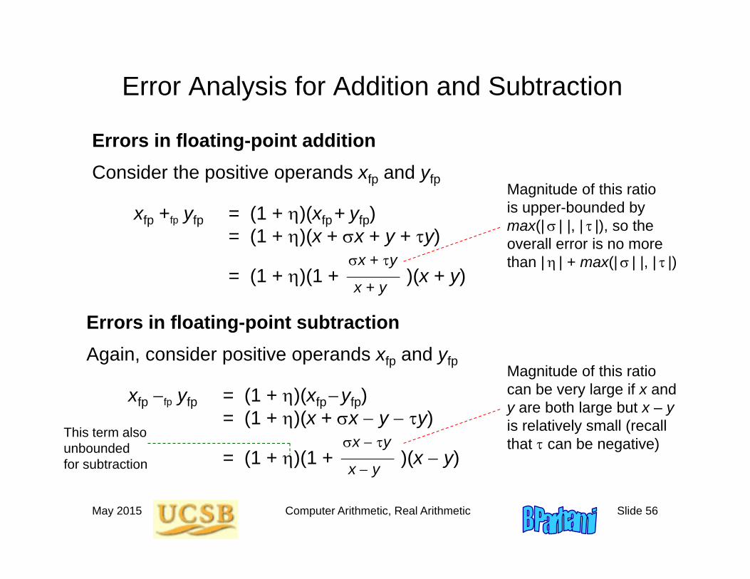
Error Analysis for Addition and Subtraction
Errors in floating-point additionConsider the positive operands xfp and yfp
xfp +fp yfp = (1 + )(xfp+ yfp)= (1 + )(x + x + y + y)
x + y= (1 + )(1 + )(x + y)
x + y
Errors in floating-point subtractionAgain, consider positive operands xfp and yfp
xfp fp yfp = (1 + )(xfpyfp)= (1 + )(x + x y y)
x y= (1 + )(1 + )(x y)
x y
Magnitude of this ratio is upper-bounded by max(| | |, | |), so the overall error is no more than | | + max(| | |, | |)
Magnitude of this ratio can be very large if x and y are both large but x – yis relatively small (recall that can be negative)
This term also unbounded for subtraction
May 2015 Computer Arithmetic, Real Arithmetic Slide 57
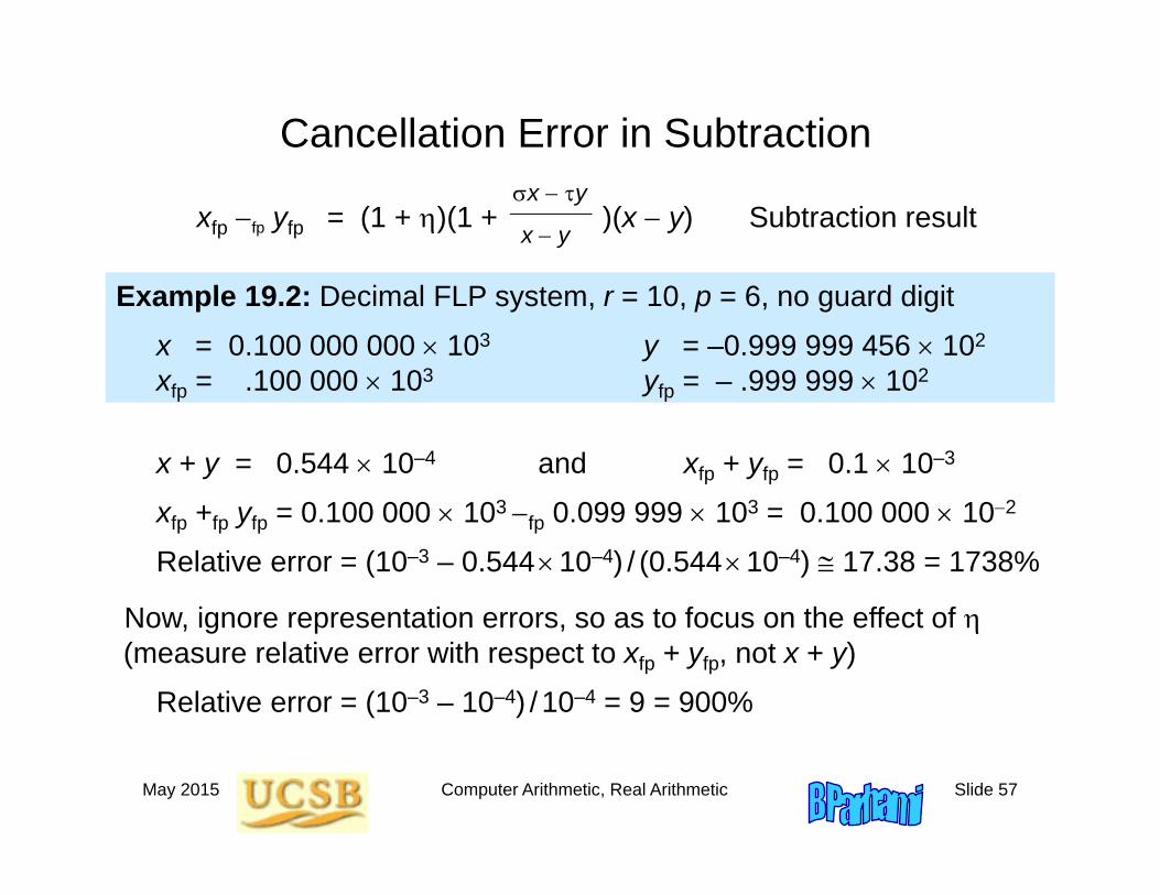
Cancellation Error in Subtractionx y
xfp fp yfp = (1 + )(1 + )(x y) Subtraction resultx y
Example 19.2: Decimal FLP system, r = 10, p = 6, no guard digit
x = 0.100 000 000 103 y = –0.999 999 456 102
xfp = .100 000 103 yfp = – .999 999 102
x + y = 0.544 10–4 and xfp + yfp = 0.1 10–3
xfp +fp yfp = 0.100 000 103 fp 0.099 999 103 = 0.100 000 102
Relative error = (10–3 – 0.54410–4) / (0.54410–4) 17.38 = 1738%
Now, ignore representation errors, so as to focus on the effect of (measure relative error with respect to xfp + yfp, not x + y)
Relative error = (10–3 – 10–4) / 10–4 = 9 = 900%
May 2015 Computer Arithmetic, Real Arithmetic Slide 58
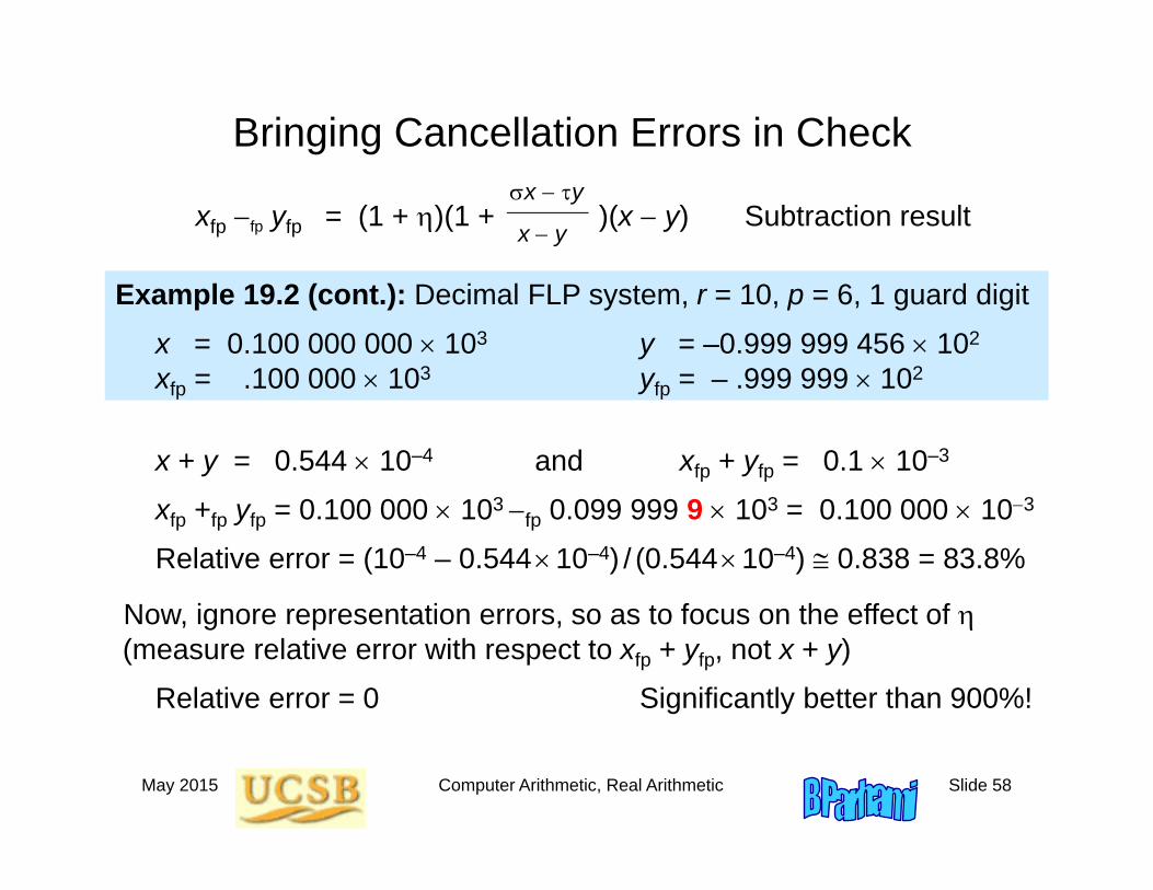
Bringing Cancellation Errors in Checkx y
xfp fp yfp = (1 + )(1 + )(x y) Subtraction resultx y
Example 19.2 (cont.): Decimal FLP system, r = 10, p = 6, 1 guard digit
x = 0.100 000 000 103 y = –0.999 999 456 102
xfp = .100 000 103 yfp = – .999 999 102
x + y = 0.544 10–4 and xfp + yfp = 0.1 10–3
xfp +fp yfp = 0.100 000 103 fp 0.099 999 9 103 = 0.100 000 103
Relative error = (10–4 – 0.54410–4) / (0.54410–4) 0.838 = 83.8%
Now, ignore representation errors, so as to focus on the effect of (measure relative error with respect to xfp + yfp, not x + y)
Relative error = 0 Significantly better than 900%!
May 2015 Computer Arithmetic, Real Arithmetic Slide 59
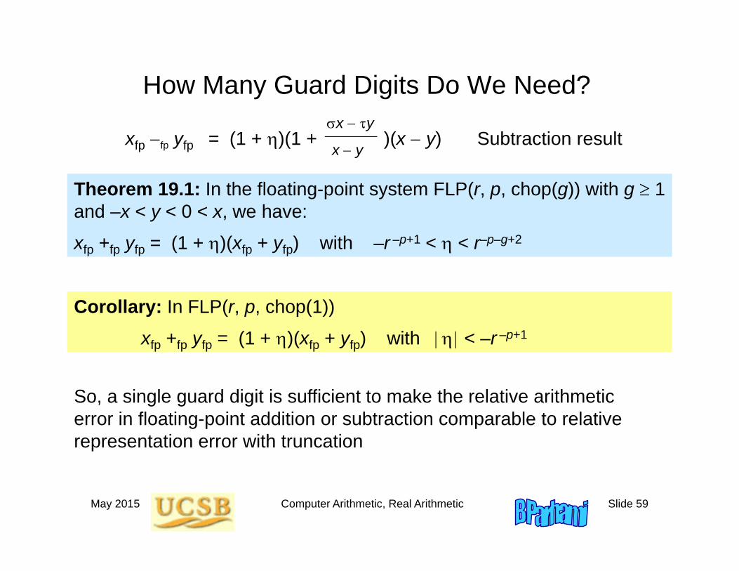
How Many Guard Digits Do We Need?x y
xfp fp yfp = (1 + )(1 + )(x y) Subtraction resultx y
Theorem 19.1: In the floating-point system FLP(r, p, chop(g)) with g 1 and –x < y < 0 < x, we have:
xfp +fp yfp = (1 + )(xfp + yfp) with –r –p+1 < < r–p–g+2
So, a single guard digit is sufficient to make the relative arithmetic error in floating-point addition or subtraction comparable to relative representation error with truncation
Corollary: In FLP(r, p, chop(1))
xfp +fp yfp = (1 + )(xfp + yfp) with < –r –p+1
May 2015 Computer Arithmetic, Real Arithmetic Slide 60
19.2 Invalidated Laws of Algebra
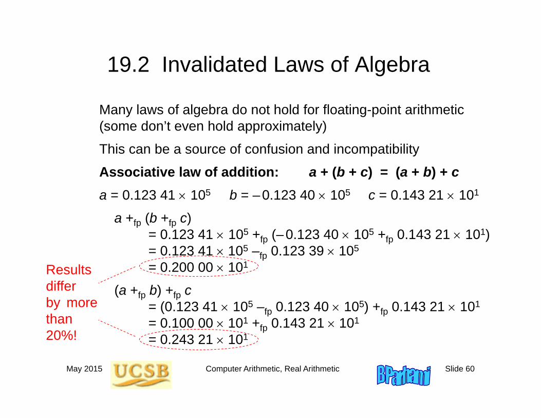
Many laws of algebra do not hold for floating-point arithmetic (some don’t even hold approximately)
This can be a source of confusion and incompatibility
Associative law of addition: a + (b + c) = (a + b) + ca = 0.123 41 105 b = –0.123 40 105 c = 0.143 21 101
a +fp (b +fp c) = 0.123 41 105 +fp (–0.123 40 105 +fp 0.143 21 101) = 0.123 41 105 –fp 0.123 39 105
= 0.200 00 101
(a +fp b) +fp c= (0.123 41 105 –fp 0.123 40 105) +fp 0.143 21 101
= 0.100 00 101 +fp 0.143 21 101
= 0.243 21 101
Resultsdifferby morethan20%!
May 2015 Computer Arithmetic, Real Arithmetic Slide 61
Elaboration on the Non-Associativity of Addition
Denser Denser Sparser Sparser
Negative numbers FLP FLP 0 +
–
Overflow region
Overflow region
Underflow regions
Positive numbers
Underflow example
Overflow example
Midway example
Typical example
min max min max + + – – – +
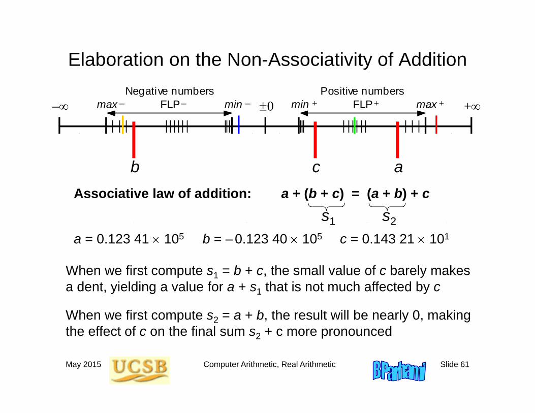
Associative law of addition: a + (b + c) = (a + b) + c
a = 0.123 41 105 b = –0.123 40 105 c = 0.143 21 101
acb
When we first compute s1 = b + c, the small value of c barely makes a dent, yielding a value for a + s1 that is not much affected by c
When we first compute s2 = a + b, the result will be nearly 0, making the effect of c on the final sum s2 + c more pronounced
s1 s2
May 2015 Computer Arithmetic, Real Arithmetic Slide 62
Do Guard Digits Help with Laws of Algebra?
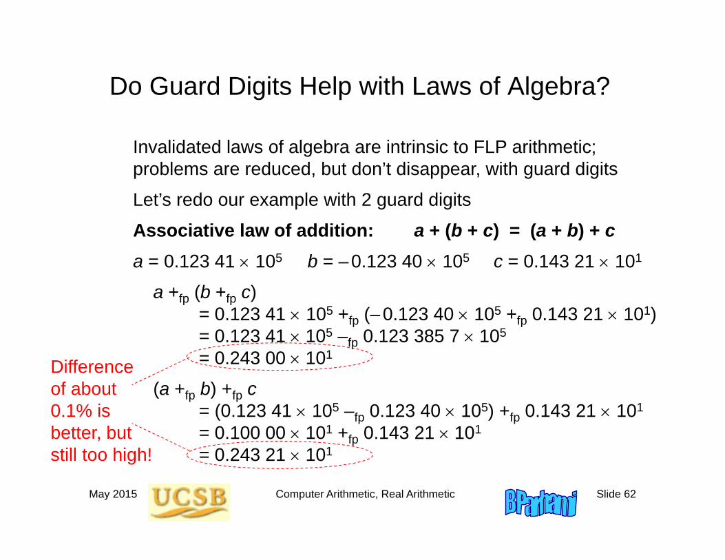
Invalidated laws of algebra are intrinsic to FLP arithmetic; problems are reduced, but don’t disappear, with guard digits
Let’s redo our example with 2 guard digits
Associative law of addition: a + (b + c) = (a + b) + ca = 0.123 41 105 b = –0.123 40 105 c = 0.143 21 101
a +fp (b +fp c) = 0.123 41 105 +fp (–0.123 40 105 +fp 0.143 21 101) = 0.123 41 105 –fp 0.123 385 7 105
= 0.243 00 101
(a +fp b) +fp c= (0.123 41 105 –fp 0.123 40 105) +fp 0.143 21 101
= 0.100 00 101 +fp 0.143 21 101
= 0.243 21 101
Difference of about 0.1% is better, but still too high!
May 2015 Computer Arithmetic, Real Arithmetic Slide 63
Unnormalized Floating-Point Arithmetic
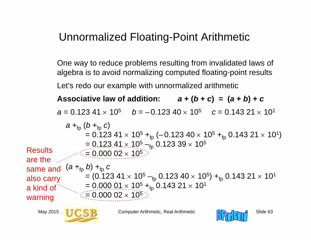
One way to reduce problems resulting from invalidated laws of algebra is to avoid normalizing computed floating-point results
Let’s redo our example with unnormalized arithmetic
Associative law of addition: a + (b + c) = (a + b) + ca = 0.123 41 105 b = –0.123 40 105 c = 0.143 21 101
a +fp (b +fp c) = 0.123 41 105 +fp (–0.123 40 105 +fp 0.143 21 101) = 0.123 41 105 –fp 0.123 39 105
= 0.000 02 105
(a +fp b) +fp c= (0.123 41 105 –fp 0.123 40 105) +fp 0.143 21 101
= 0.000 01 105 +fp 0.143 21 101
= 0.000 02 105
Results are the same and also carry a kind of warning
May 2015 Computer Arithmetic, Real Arithmetic Slide 64
Other Invalidated Laws of Algebra with FLP Arithmetic
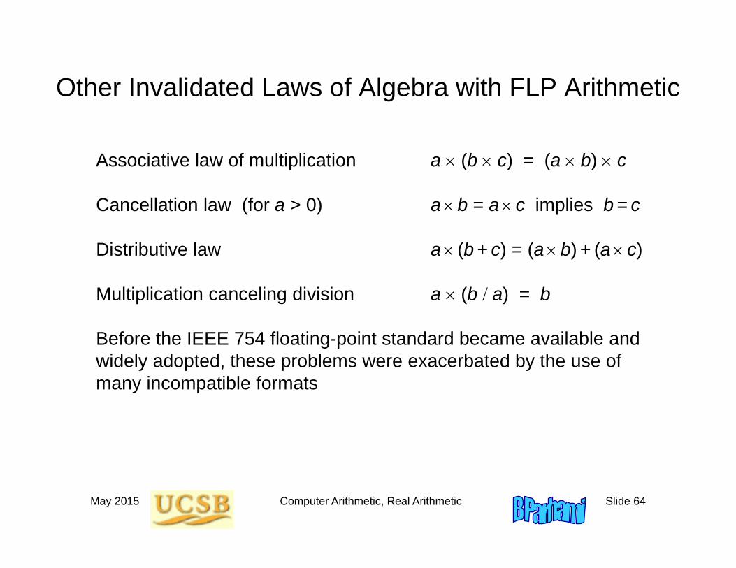
Associative law of multiplication a (b c) = (a b) c
Cancellation law (for a > 0) a b = a c implies b = c
Distributive law a (b + c) = (a b) + (a c)
Multiplication canceling division a (b a) = b
Before the IEEE 754 floating-point standard became available and widely adopted, these problems were exacerbated by the use of many incompatible formats
May 2015 Computer Arithmetic, Real Arithmetic Slide 65
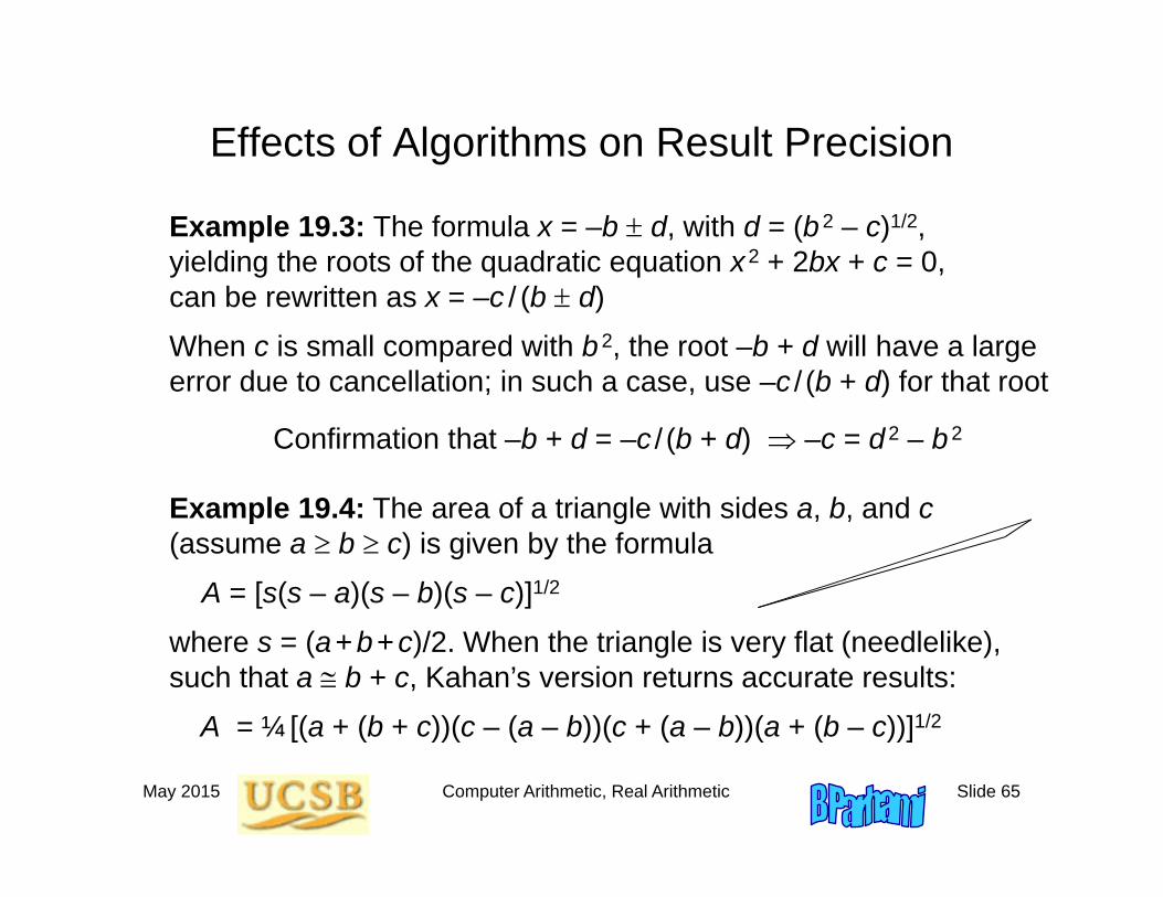
Effects of Algorithms on Result Precision
Example 19.3: The formula x = –b d, with d = (b 2 – c)1/2, yielding the roots of the quadratic equation x 2 + 2bx + c = 0, can be rewritten as x = –c / (b d)
When c is small compared with b 2, the root –b + d will have a large error due to cancellation; in such a case, use –c / (b + d) for that root
Example 19.4: The area of a triangle with sides a, b, and c(assume a b c) is given by the formula
A = [s(s – a)(s – b)(s – c)]1/2
where s = (a+b+c)/2. When the triangle is very flat (needlelike), such that a b + c, Kahan’s version returns accurate results:
A = ¼[(a + (b + c))(c – (a – b))(c + (a – b))(a + (b – c))]1/2
Confirmation that –b + d = –c / (b + d) –c = d 2 – b 2
May 2015 Computer Arithmetic, Real Arithmetic Slide 66
19.3 Worst-Case Error AccumulationIn a sequence of operations, round-off errors might add up
The larger the number of cascaded computation steps (that depend on results from previous steps), the greater the chance for, and the magnitude of, accumulated errors
With rounding, errors of opposite signs tend to cancel each other out in the long run, but one cannot count on such cancellations
Practical implications:Perform intermediate computations with a higher precision than what is required in the final result
Implement multiply-accumulate in hardware (DSP chips)
Reduce the number of cascaded arithmetic operations; So, using computationally more efficient algorithms has the double benefit of reducing the execution time as well as accumulated errors
May 2015 Computer Arithmetic, Real Arithmetic Slide 67
Example: Inner-Product Calculation
Consider the computation z = x(i) y(i), for i [0, 1023]
Max error per multiply-add step = ulp/2 + ulp/2 = ulp
Total worst-case absolute error = 1024 ulp(equivalent to losing 10 bits of precision)
A possible cure: keep the double-width products in their entirety and add them to compute a double-width result which is rounded to single-width at the very last step
Multiplications do not introduce any round-off error Max error per addition = ulp2/2Total worst-case error = 1024 ulp2/2 + ulp/2
Therefore, provided that overflow is not a problem, a highly accurate result is obtained
May 2015 Computer Arithmetic, Real Arithmetic Slide 68
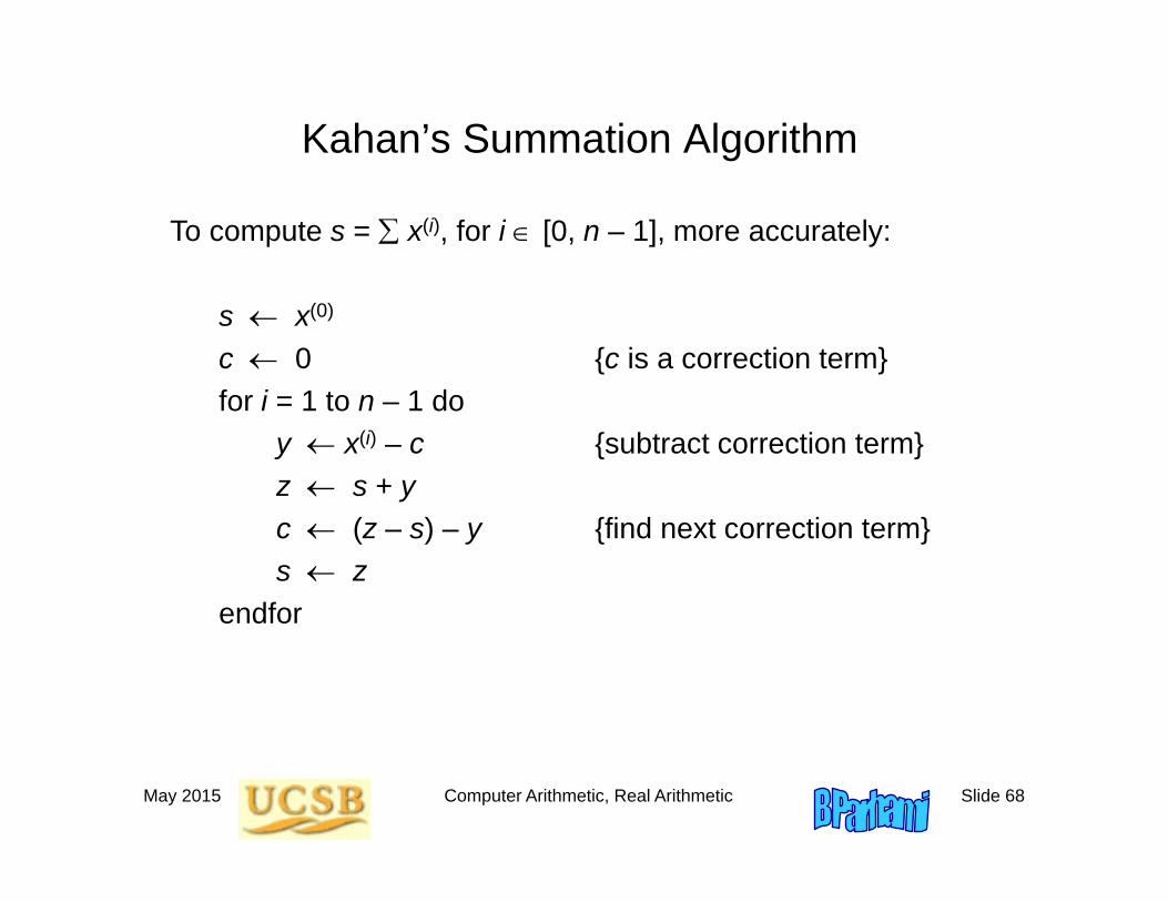
Kahan’s Summation Algorithm
To compute s = x(i), for i [0, n – 1], more accurately:
s x(0)
c 0 {c is a correction term}for i = 1 to n – 1 do
y x(i) – c {subtract correction term}z s + yc (z – s) – y {find next correction term}s z
endfor
May 2015 Computer Arithmetic, Real Arithmetic Slide 69
19.4 Error Distribution and Expected Errors
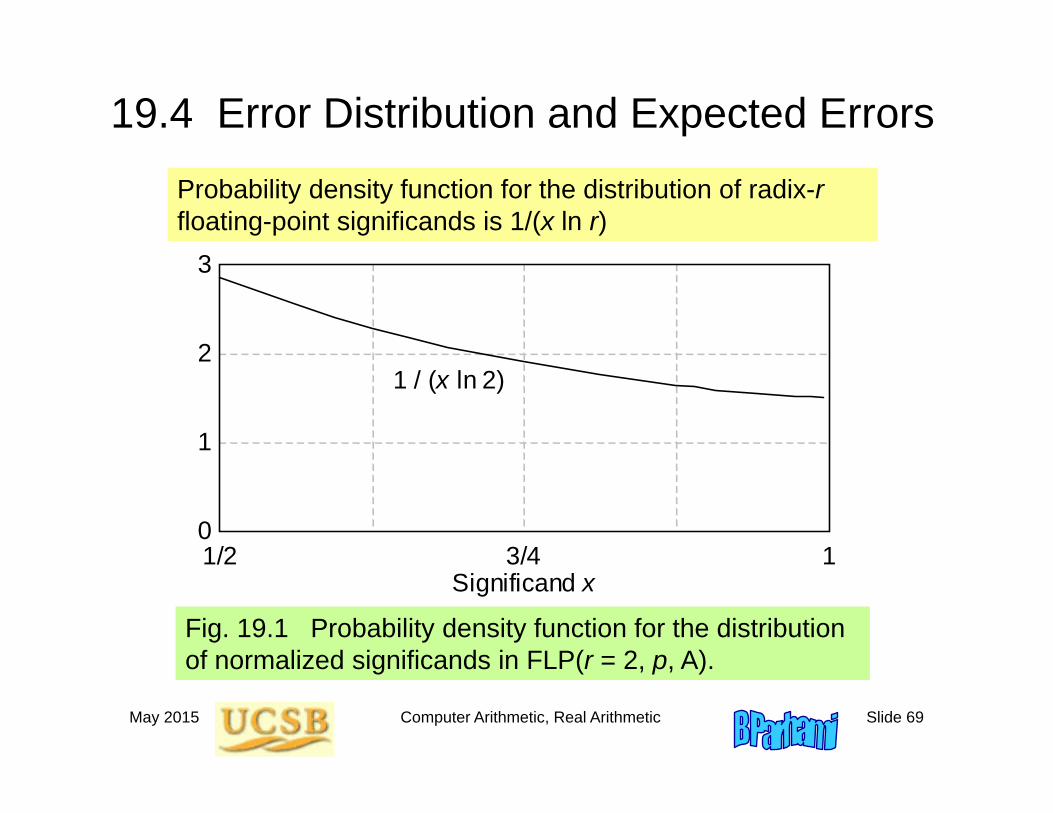
Fig. 19.1 Probability density function for the distribution of normalized significands in FLP(r = 2, p, A).
Probability density function for the distribution of radix-rfloating-point significands is 1/(x ln r)
0
1
2
3
1/2 1 3/4 Significand x
1 / (x ln 2)
May 2015 Computer Arithmetic, Real Arithmetic Slide 70
Maximum Relative Representation Error
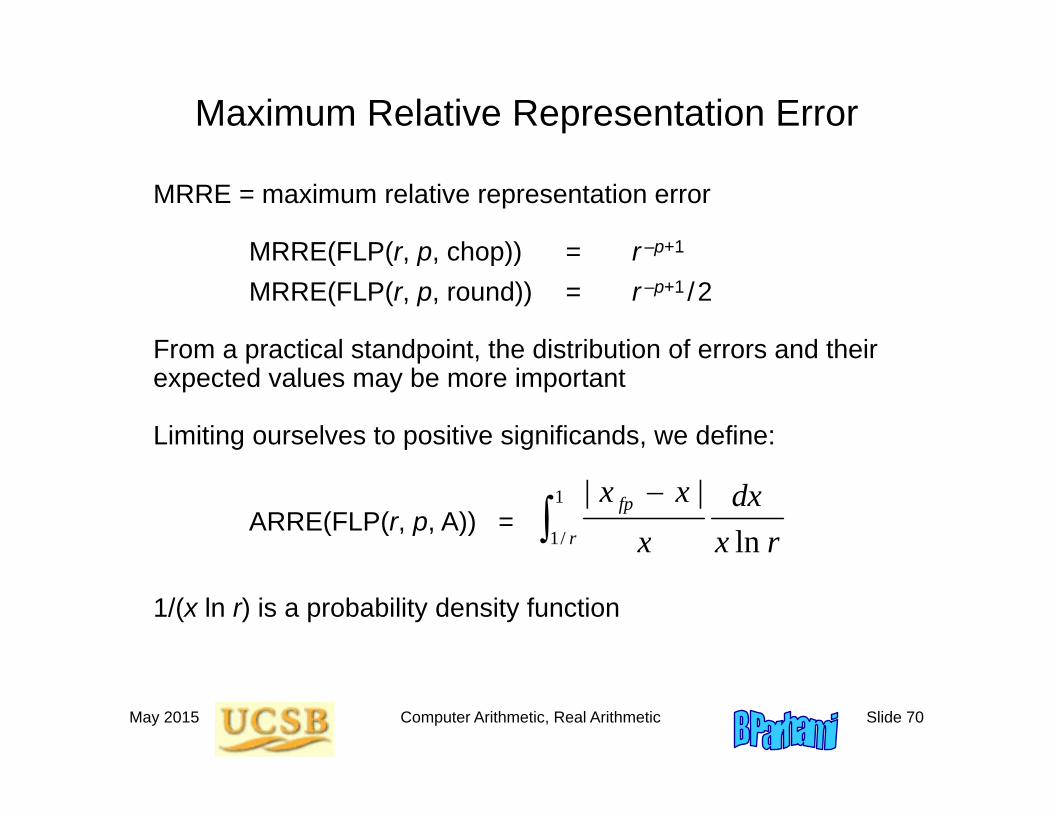
MRRE = maximum relative representation error
MRRE(FLP(r, p, chop)) = r –p+1
MRRE(FLP(r, p, round)) = r –p+1 /2
From a practical standpoint, the distribution of errors and their expected values may be more important
Limiting ourselves to positive significands, we define:
ARRE(FLP(r, p, A)) =
1/(x ln r) is a probability density function
rxdx
xxx
r
fp
ln||1
/1
May 2015 Computer Arithmetic, Real Arithmetic Slide 71
19.5 Forward Error Analysis
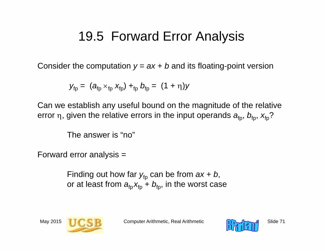
Consider the computation y = ax + b and its floating-point version
yfp = (afp fp xfp) +fp bfp = (1 + )y
Can we establish any useful bound on the magnitude of the relative error , given the relative errors in the input operands afp, bfp, xfp?
The answer is “no”
Forward error analysis =
Finding out how far yfp can be from ax + b, or at least from afpxfp + bfp, in the worst case
May 2015 Computer Arithmetic, Real Arithmetic Slide 72
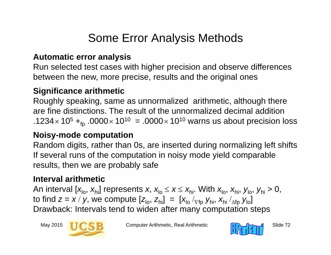
Some Error Analysis MethodsAutomatic error analysisRun selected test cases with higher precision and observe differences between the new, more precise, results and the original ones
Significance arithmeticRoughly speaking, same as unnormalized arithmetic, although there are fine distinctions. The result of the unnormalized decimal addition .1234105 +fp .00001010 = .00001010 warns us about precision loss
Noisy-mode computationRandom digits, rather than 0s, are inserted during normalizing left shifts If several runs of the computation in noisy mode yield comparable results, then we are probably safe
Interval arithmeticAn interval [xlo, xhi] represents x, xlo x xhi. With xlo, xhi, ylo, yhi > 0, to find z = x y, we compute [zlo, zhi] = [xlo fp yhi, xhi fp ylo] Drawback: Intervals tend to widen after many computation steps
May 2015 Computer Arithmetic, Real Arithmetic Slide 73
19.6 Backward Error Analysis
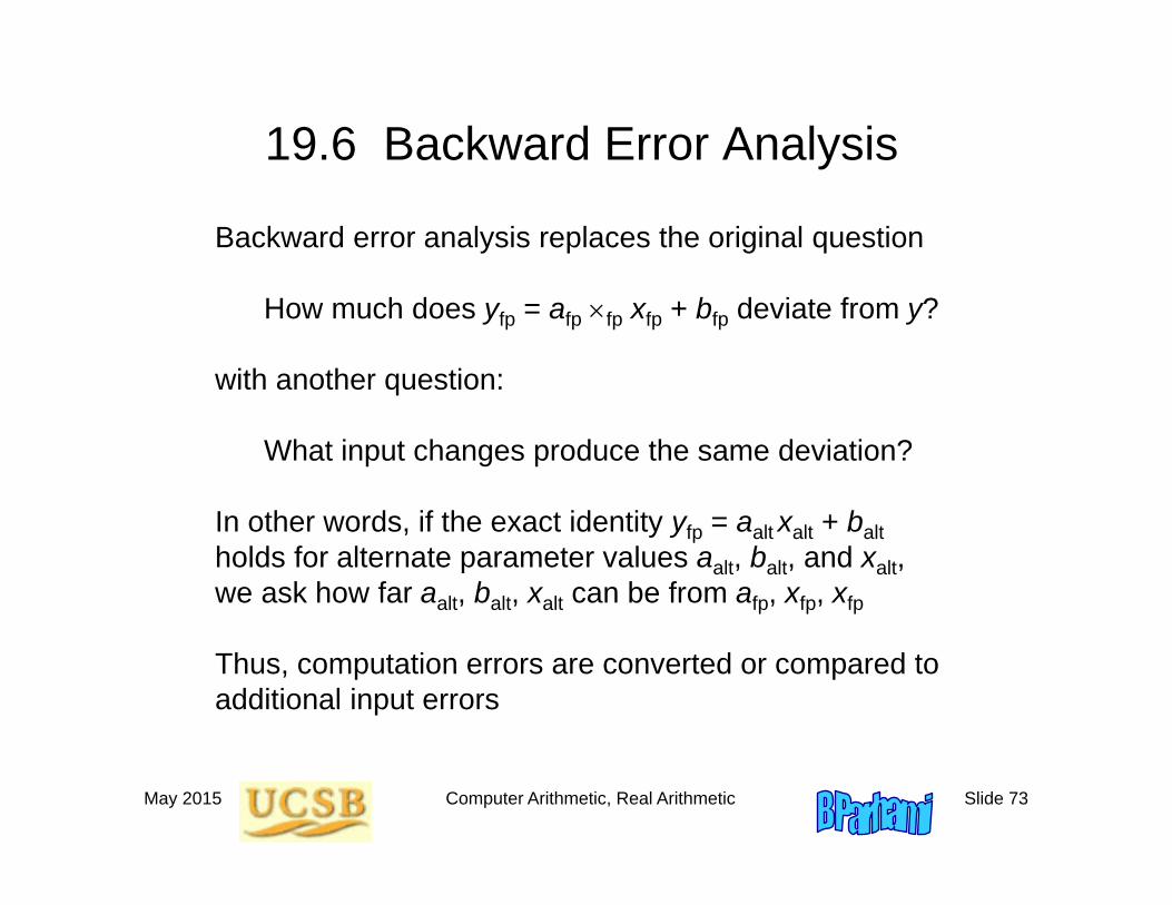
Backward error analysis replaces the original question
How much does yfp = afp fp xfp + bfp deviate from y?
with another question:
What input changes produce the same deviation?
In other words, if the exact identity yfp = aalt xalt + baltholds for alternate parameter values aalt, balt, and xalt, we ask how far aalt, balt, xalt can be from afp, xfp, xfp
Thus, computation errors are converted or compared to additional input errors
May 2015 Computer Arithmetic, Real Arithmetic Slide 74
Example of Backward Error Analysis
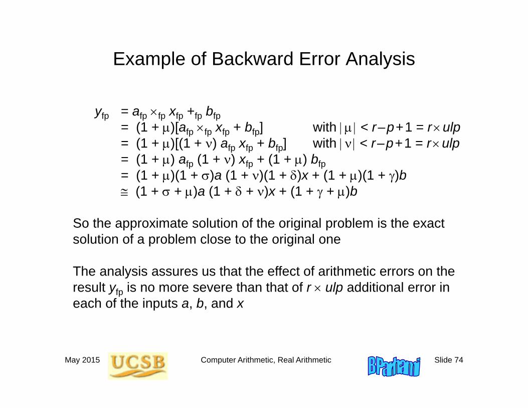
yfp = afp fp xfp +fp bfp= (1 + )[afp fp xfp + bfp] with < r–p+1 = rulp= (1 + )[(1 + ) afp xfp + bfp] with < r–p+1 = rulp= (1 + ) afp (1 + ) xfp + (1 + ) bfp= (1 + )(1 + )a (1 + )(1 + )x + (1 + )(1 + )b (1 + + )a (1 + + )x + (1 + + )b
So the approximate solution of the original problem is the exact solution of a problem close to the original one
The analysis assures us that the effect of arithmetic errors on the result yfp is no more severe than that of r ulp additional error in each of the inputs a, b, and x
May 2015 Computer Arithmetic, Real Arithmetic Slide 75
20 Precise and Certifiable Arithmetic
Chapter GoalsDiscuss methods for doing arithmeticwhen results of high accuracyor guaranteed correctness are required
Chapter HighlightsMore precise computation through
multi- or variable-precision arithmeticResult certification by means of
exact or error-bounded arithmeticPrecise /exact arithmetic with low overhead
May 2015 Computer Arithmetic, Real Arithmetic Slide 76
Precise and Certifiable Arithmetic: Topics
Topics in This Chapter
20.1 High Precision and Certifiability
20.2 Exact Arithmetic
20.3 Multiprecision Arithmetic
20.4 Variable-Precision Arithmetic
20.5 Error-Bounding via Interval Arithmetic
20.6 Adaptive and Lazy Arithmetic
May 2015 Computer Arithmetic, Real Arithmetic Slide 77
20.1 High Precision and CertifiabilityThere are two aspects of precision to discuss:
Results possessing adequate precision
Being able to provide assurance of the same
We consider 3 distinct approaches for coping with precision issues:
1. Obtaining completely trustworthy results via exact arithmetic
2. Making the arithmetic highly precise to raise our confidence in the validity of the results: multi- or variable-precision arith
3. Doing ordinary or high-precision calculations, while tracking potential error accumulation (can lead to fail-safe operation)
We take the hardware to be completely trustworthyHardware reliability issues dealt with in Chapter 27
May 2015 Computer Arithmetic, Real Arithmetic Slide 78
20.2 Exact Arithmetic
x pq a 0
1
a1 1
a 2 1
1
a m 1 1
a m
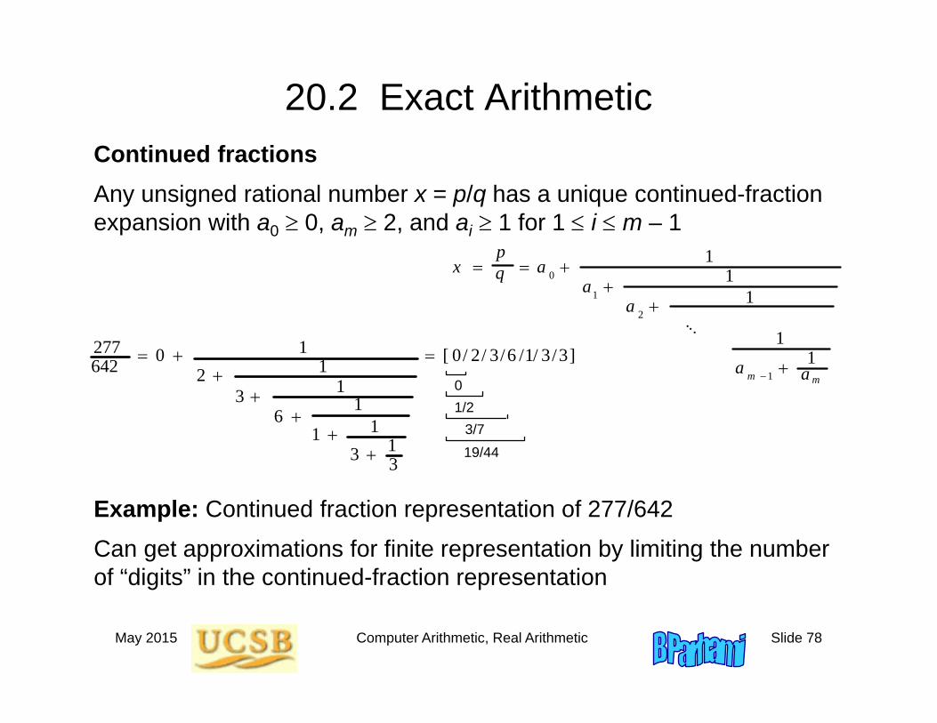
Continued fractionsAny unsigned rational number x = p/q has a unique continued-fraction expansion with a0 0, am 2, and ai 1 for 1 i m – 1
277642 0 1
2 1
3 1
6 1
1 13 1
3
[ 0/ 2/ 3/6 /1/ 3/3]01/2
3/719/44
Example: Continued fraction representation of 277/642
Can get approximations for finite representation by limiting the number of “digits” in the continued-fraction representation
May 2015 Computer Arithmetic, Real Arithmetic Slide 79
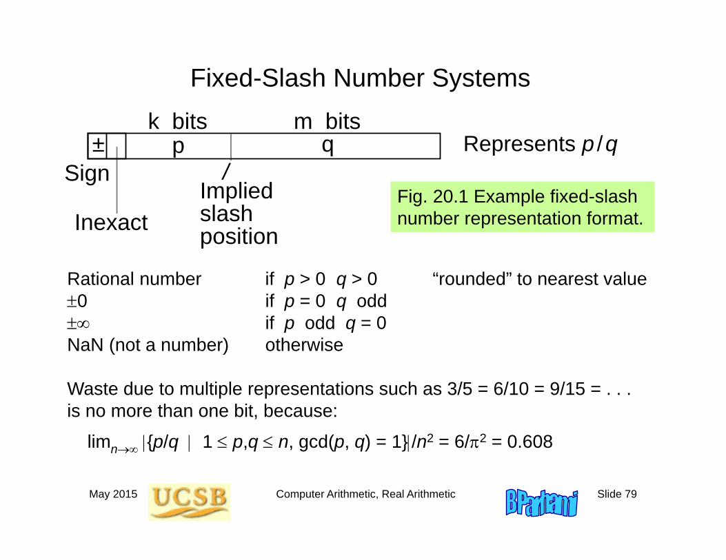
Fixed-Slash Number Systems
Rational number if p > 0 q > 0 “rounded” to nearest value0 if p = 0 q odd if p odd q = 0NaN (not a number) otherwise
SignImplied slash position
± p q
Inexact
k bits m bits
/Fig. 20.1 Example fixed-slash number representation format.
Waste due to multiple representations such as 3/5 = 6/10 = 9/15 = . . . is no more than one bit, because:
limn {p/q 1 p,q n, gcd(p, q) = 1}/n2 = 6/2 = 0.608
Represents p /q
May 2015 Computer Arithmetic, Real Arithmetic Slide 80
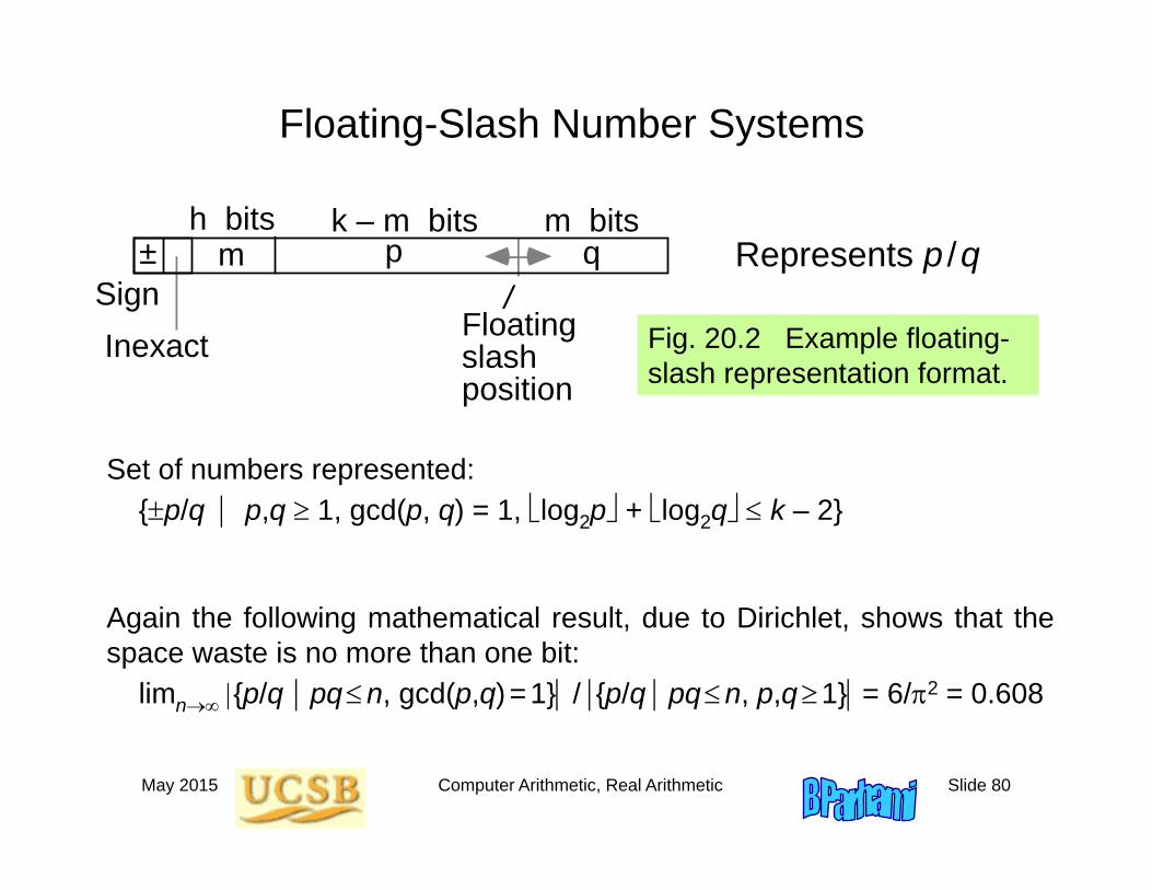
Floating-Slash Number Systems
Set of numbers represented:{p/q p,q 1, gcd(p, q) = 1, log2p + log2q k – 2}
Fig. 20.2 Example floating-slash representation format.
Again the following mathematical result, due to Dirichlet, shows that thespace waste is no more than one bit:
limn {p/q pqn, gcd(p,q)=1} / {p/q pqn, p,q1} = 6/2 = 0.608
Represents p /qSign
± p q
Inexact
m bitsh bitsm
Floating slash position
k – m bits
/
May 2015 Computer Arithmetic, Real Arithmetic Slide 81
20.3 Multiprecision Arithmetic
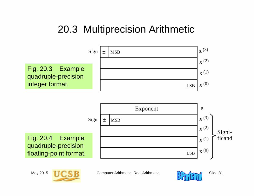
Fig. 20.3 Example quadruple-precision integer format.
Fig. 20.4 Example quadruple-precision floating-point format.
Sign ± MSB
LSB
x
x
x
x
(3)
(2)
(1)
(0)
Sign ± MSB x
x
x
x
(3)
(2)
(1)
(0)
Exponent
LSB
e
Signi- ficand
May 2015 Computer Arithmetic, Real Arithmetic Slide 82
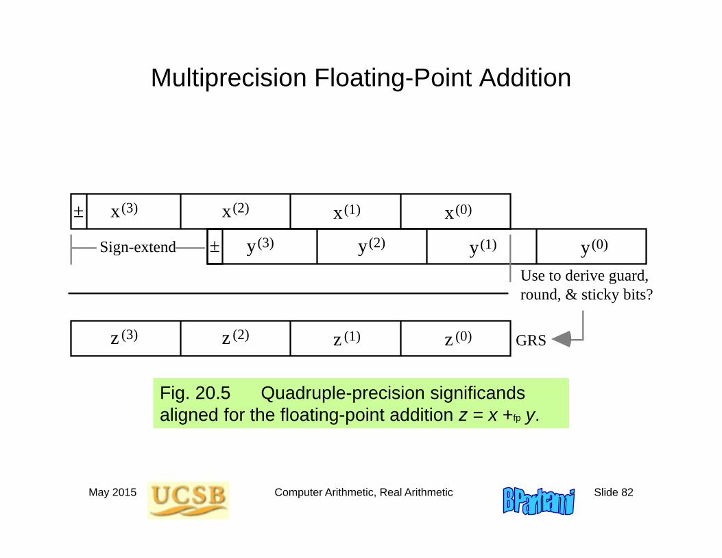
Multiprecision Floating-Point Addition
Fig. 20.5 Quadruple-precision significands aligned for the floating-point addition z = x +fp y.
± x x x x(3) (2) (1) (0)
y y y y(3) (2) (1) (0)
z z z z(3) (2) (1) (0)
Use to derive guard, round, & sticky bits?
Sign-extend ±
GRS
May 2015 Computer Arithmetic, Real Arithmetic Slide 83
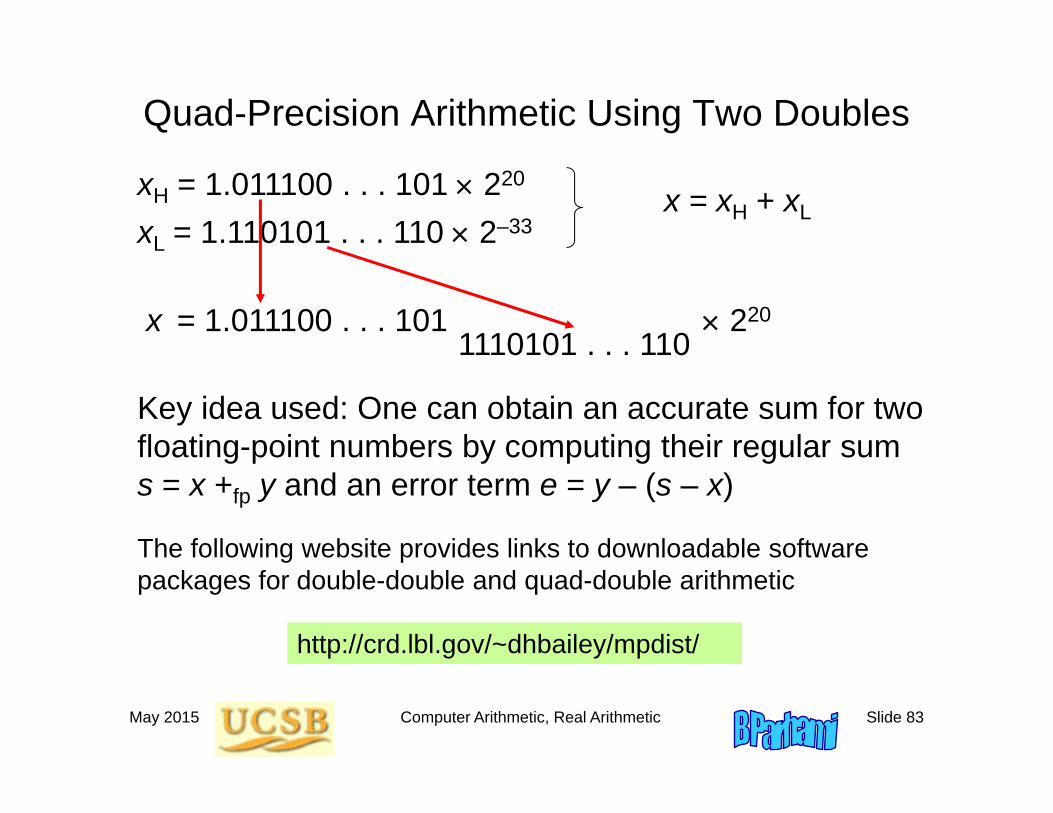
Quad-Precision Arithmetic Using Two Doubles
http://crd.lbl.gov/~dhbailey/mpdist/
xH = 1.011100 . . . 101 220
xL = 1.110101 . . . 110 2–33 x = xH + xL
x = 1.011100 . . . 101 220
The following website provides links to downloadable software packages for double-double and quad-double arithmetic
Key idea used: One can obtain an accurate sum for two floating-point numbers by computing their regular sum s = x +fp y and an error term e = y – (s – x)
1110101 . . . 110
May 2015 Computer Arithmetic, Real Arithmetic Slide 84
20.4 Variable-Precision Arithmetic
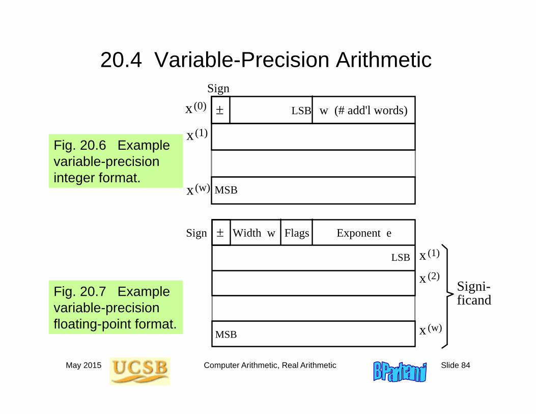
Fig. 20.6 Example variable-precision integer format.
Sign
±
MSB
LSBx
x
x
(0)
(1)
(w)
w (# add'l words)
Fig. 20.7 Example variable-precision floating-point format.
Sign ±
MSB
x
x
x
(1)
(2)
(w)
Exponent e
LSB
Signi- ficand
Width w Flags
May 2015 Computer Arithmetic, Real Arithmetic Slide 85
Variable-Precision Floating-Point Addition
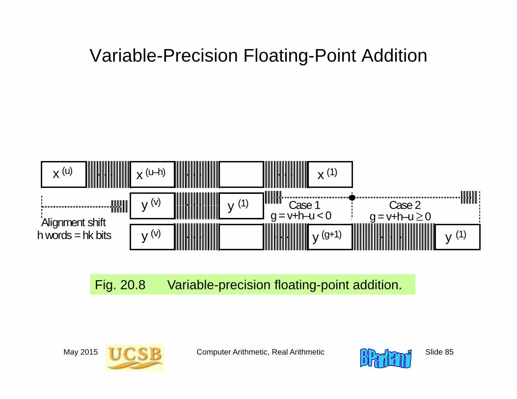
Fig. 20.8 Variable-precision floating-point addition.
x x x(u) (u–h) (1)
h words = hk bits y y(v) (1)
y (v) y (1) Case 2Case 1 g = v+h–u 0g = v+h–u < 0
y (g+1)Alignment shift
. . .
. . .. . .. . .
. . .
. . .. . .
May 2015 Computer Arithmetic, Real Arithmetic Slide 86
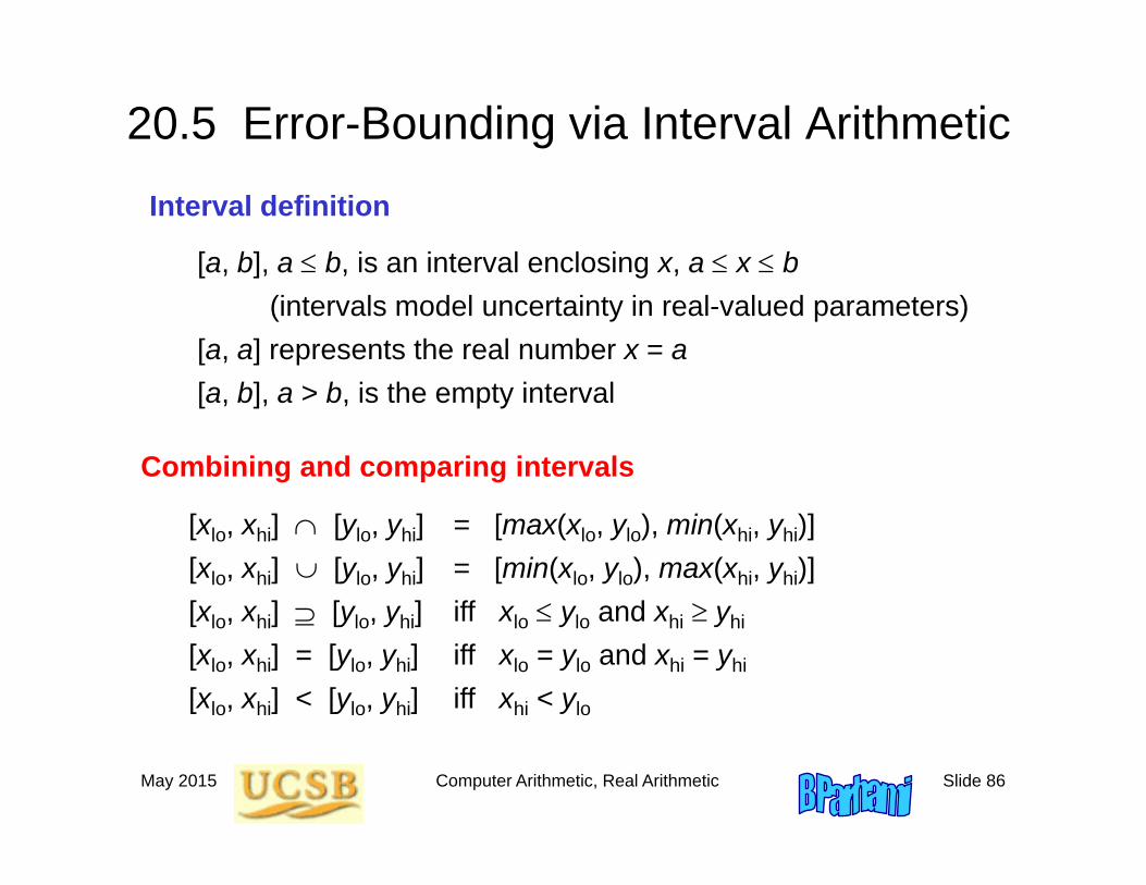
20.5 Error-Bounding via Interval ArithmeticInterval definition
[a, b], a b, is an interval enclosing x, a x b (intervals model uncertainty in real-valued parameters)
[a, a] represents the real number x = a[a, b], a > b, is the empty interval
Combining and comparing intervals
[xlo, xhi] [ylo, yhi] = [max(xlo, ylo), min(xhi, yhi)][xlo, xhi] [ylo, yhi] = [min(xlo, ylo), max(xhi, yhi)][xlo, xhi] [ylo, yhi] iff xlo ylo and xhi yhi
[xlo, xhi] = [ylo, yhi] iff xlo = ylo and xhi = yhi
[xlo, xhi] < [ylo, yhi] iff xhi < ylo
May 2015 Computer Arithmetic, Real Arithmetic Slide 87
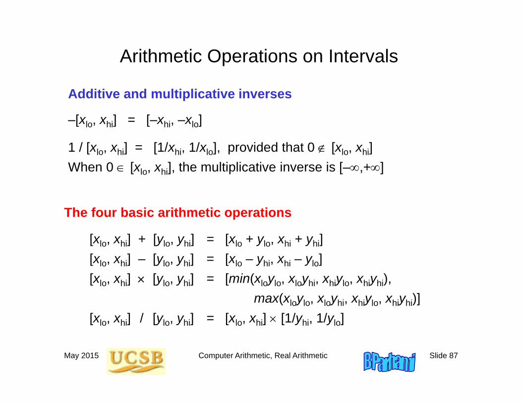
Arithmetic Operations on Intervals
Additive and multiplicative inverses
–[xlo, xhi] = [–xhi, –xlo]
1 / [xlo, xhi] = [1/xhi, 1/xlo], provided that 0 [xlo, xhi] When 0 [xlo, xhi], the multiplicative inverse is [–,+]
The four basic arithmetic operations
[xlo, xhi] + [ylo, yhi] = [xlo + ylo, xhi + yhi][xlo, xhi] – [ylo, yhi] = [xlo – yhi, xhi – ylo][xlo, xhi] [ylo, yhi] = [min(xloylo, xloyhi, xhiylo, xhiyhi),
max(xloylo, xloyhi, xhiylo, xhiyhi)][xlo, xhi] / [ylo, yhi] = [xlo, xhi] [1/yhi, 1/ylo]
May 2015 Computer Arithmetic, Real Arithmetic Slide 88
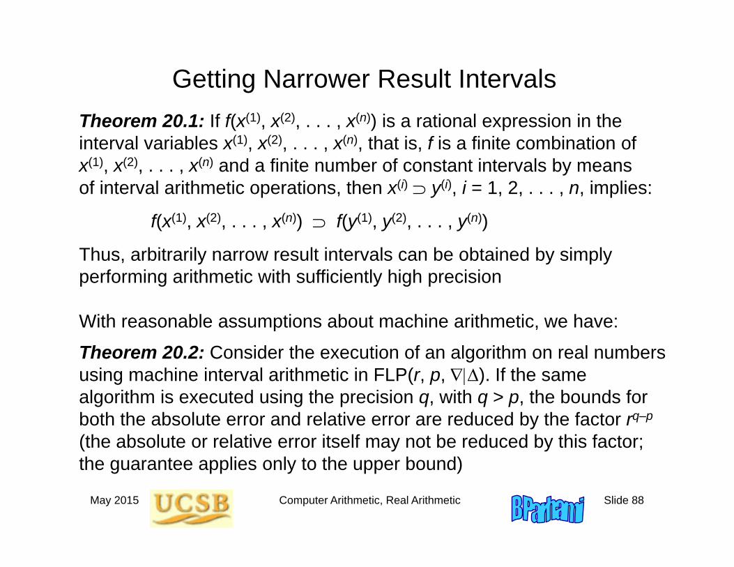
Getting Narrower Result Intervals
With reasonable assumptions about machine arithmetic, we have:
Theorem 20.2: Consider the execution of an algorithm on real numbers using machine interval arithmetic in FLP(r, p, ). If the same algorithm is executed using the precision q, with q > p, the bounds for both the absolute error and relative error are reduced by the factor rq–p
(the absolute or relative error itself may not be reduced by this factor; the guarantee applies only to the upper bound)
Theorem 20.1: If f(x(1), x(2), . . . , x(n)) is a rational expression in the interval variables x(1), x(2), . . . , x(n), that is, f is a finite combination of x(1), x(2), . . . , x(n) and a finite number of constant intervals by means of interval arithmetic operations, then x(i) y(i), i = 1, 2, . . . , n, implies:
f(x(1), x(2), . . . , x(n)) f(y(1), y(2), . . . , y(n))
Thus, arbitrarily narrow result intervals can be obtained by simply performing arithmetic with sufficiently high precision
May 2015 Computer Arithmetic, Real Arithmetic Slide 89
A Strategy for Accurate Interval Arithmetic
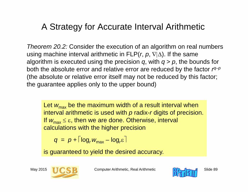
Theorem 20.2: Consider the execution of an algorithm on real numbers using machine interval arithmetic in FLP(r, p, ). If the same algorithm is executed using the precision q, with q > p, the bounds for both the absolute error and relative error are reduced by the factor rq–p
(the absolute or relative error itself may not be reduced by this factor; the guarantee applies only to the upper bound)
Let wmax be the maximum width of a result interval when interval arithmetic is used with p radix-r digits of precision. If wmax , then we are done. Otherwise, interval calculations with the higher precision
q = p + logr wmax – logr
is guaranteed to yield the desired accuracy.
May 2015 Computer Arithmetic, Real Arithmetic Slide 90
The Interval Newton Method1/x – d
x65432100
–1
2
1
I (0)
N(I(0))I (1)
Slope = –1/4
Slope = –4
A
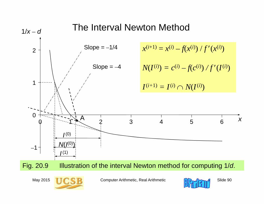
Fig. 20.9 Illustration of the interval Newton method for computing 1/d.
x(i+1) = x(i) – f(x(i)) / f (x(i))
N(I (i)) = c(i) – f(c(i)) / f (I (i))
I (i+1) = I (i) N(I (i))
May 2015 Computer Arithmetic, Real Arithmetic Slide 91
Laws of Algebra in Interval Arithmetic
As in FLP arithmetic, laws of algebra may not hold for interval arithmetic
For example, one can readily construct an example where for intervals x, y and z, the following two expressions yield different interval results, thus demonstrating the violation of the distributive law:
x(y + z) xy + xz
Can you find other laws of algebra that may be violated?
May 2015 Computer Arithmetic, Real Arithmetic Slide 92
20.6 Adaptive and Lazy Arithmetic
Need-based incremental precision adjustment to avoid high-precision calculations dictated by worst-case errors
Lazy evaluation is a powerful paradigm that has been and is being used in many different contexts. For example, in evaluating composite conditionals such as
if cond1 and cond2 then action
evaluation of cond2 may be skipped if cond1 yields “false”More generally, lazy evaluation means
postponing all computations or actions until they become irrelevant or unavoidable
Opposite of lazy evaluation (speculative or aggressive execution) has been applied extensively
May 2015 Computer Arithmetic, Real Arithmetic Slide 93
Lazy Arithmetic with Redundant Representations
Redundant number representations offer some advantages for lazy arithmetic
Because redundant representations support MSD-first arithmetic, it is possible to produce a small number of result digits by using correspondingly less computational effort, until more precision is actually needed