Embed Size (px)
Citation preview
Apr. 2011 Computer Arithmetic, Division Slide 1
Part IVDivision
Number Representation Numbers and Arithmetic Representing Signed Numbers Redundant Number Systems Residue Number Systems
Addition / Subtraction Basic Addition and Counting Carry-Lookahead Adders Variations in Fast Adders Multioperand Addition
Multiplication Basic Multiplication Schemes High-Radix Multipliers Tree and Array Multipliers Variations in Multipliers
Division Basic Division Schemes High-Radix Dividers Variations in Dividers Division by Convergence
Real Arithmetic Floating-Point Reperesentations Floating-Point Operations Errors and Error Control Precise and Certifiable Arithmetic
Function Evaluation Square-Rooting Methods The CORDIC Algorithms Variations in Function Evaluation Arithmetic by Table Lookup
Implementation Topics High-Throughput Arithmetic Low-Power Arithmetic Fault-Tolerant Arithmetic Past, Present, and Future
Parts Chapters
I.
II.
III.
IV.
V.
VI.
VII.
1. 2. 3. 4.
5. 6. 7. 8.
9. 10. 11. 12.
25. 26. 27. 28.
21. 22. 23. 24.
17. 18. 19. 20.
13. 14. 15. 16.
Ele
men
tary
Ope
ratio
ns
28. Reconfigurable Arithmetic
Appendix: Past, Present, and Future
Apr. 2011 Computer Arithmetic, Division Slide 2
About This Presentation
Edition Released Revised Revised Revised RevisedFirst Jan. 2000 Sep. 2001 Sep. 2003 Oct. 2005 May 2007
May 2008 May 2009
Second May 2010 Apr. 2011
This presentation is intended to support the use of the textbookComputer Arithmetic: Algorithms and Hardware Designs (Oxford U. Press, 2nd ed., 2010, ISBN 978-0-19-532848-6). It is updated regularly by the author as part of his teaching of the graduate course ECE 252B, Computer Arithmetic, at the University of California, Santa Barbara. Instructors can use these slides freely in classroom teaching and for other educational purposes. Unauthorized uses are strictly prohibited. © Behrooz Parhami
Apr. 2011 Computer Arithmetic, Division Slide 3
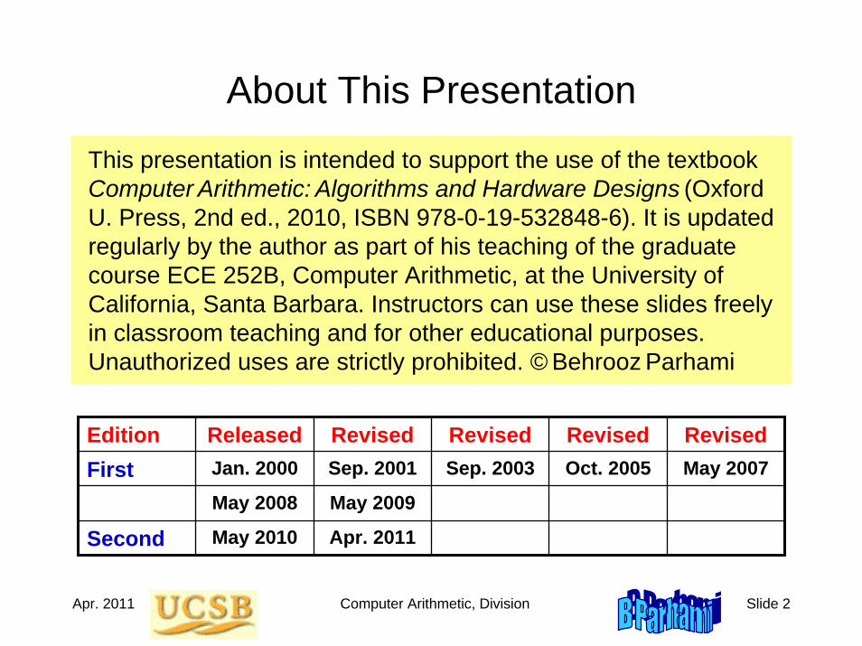
IV Division
Topics in This PartChapter 13 Basic Division SchemesChapter 14 High-Radix DividersChapter 15 Variations in DividersChapter 16 Division by Convergence
Review Division schemes and various speedup methods• Hardest basic operation (fortunately, also the rarest)• Division speedup methods: high-radix, array, . . .• Combined multiplication/division hardware • Digit-recurrence vs convergence division schemes

Apr. 2011 Computer Arithmetic, Division Slide 4
Be fruitful and multiply . . .
Now, divide.
Apr. 2011 Computer Arithmetic, Division Slide 5
13 Basic Division Schemes
Chapter GoalsStudy shift/subtract or bit-at-a-time dividersand set the stage for faster methods andvariations to be covered in Chapters 14-16
Chapter HighlightsShift/subtract divide vs shift/add multiplyHardware, firmware, software algorithmsDividing 2’s-complement numbersThe special case of a constant divisor
Apr. 2011 Computer Arithmetic, Division Slide 6
Basic Division Schemes: Topics
Topics in This Chapter
13.1 Shift/Subtract Division Algorithms
13.2 Programmed Division
13.3 Restoring Hardware Dividers
13.4 Nonrestoring and Signed Division
13.5 Division by Constants
13.6 Radix-2 SRT Division
Apr. 2011 Computer Arithmetic, Division Slide 7
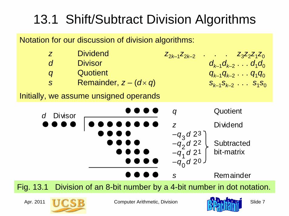
13.1 Shift/Subtract Division AlgorithmsNotation for our discussion of division algorithms:
z Dividend z2k–1z2k–2 . . . z3z2z1z0d Divisor dk–1dk–2 . . . d1d0q Quotient qk–1qk–2 . . . q1q0s Remainder, z – (d × q) sk–1sk–2 . . . s1s0
Initially, we assume unsigned operands
Fig. 13.1 Division of an 8-bit number by a 4-bit number in dot notation.
Dividend
Subtracted bit-matrix
z
s Remainder
Quotient q Divisor d
q d 2 3 3 –
q d 2 2 2 –
q d 2 1 1 –
q d 2 0 0 –
Apr. 2011 Computer Arithmetic, Division Slide 8
Division versus Multiplication
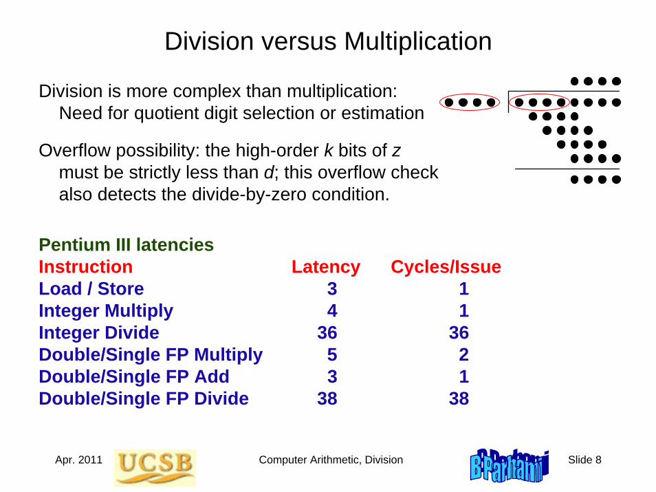
Division is more complex than multiplication:Need for quotient digit selection or estimation
Overflow possibility: the high-order k bits of zmust be strictly less than d; this overflow check also detects the divide-by-zero condition.
z
s
q Divisor d
q
Pentium III latenciesInstruction Latency Cycles/IssueLoad / Store 3 1Integer Multiply 4 1Integer Divide 36 36Double/Single FP Multiply 5 2Double/Single FP Add 3 1Double/Single FP Divide 38 38
3– q 2– q 1– q 0–
Apr. 2011 Computer Arithmetic, Division Slide 9
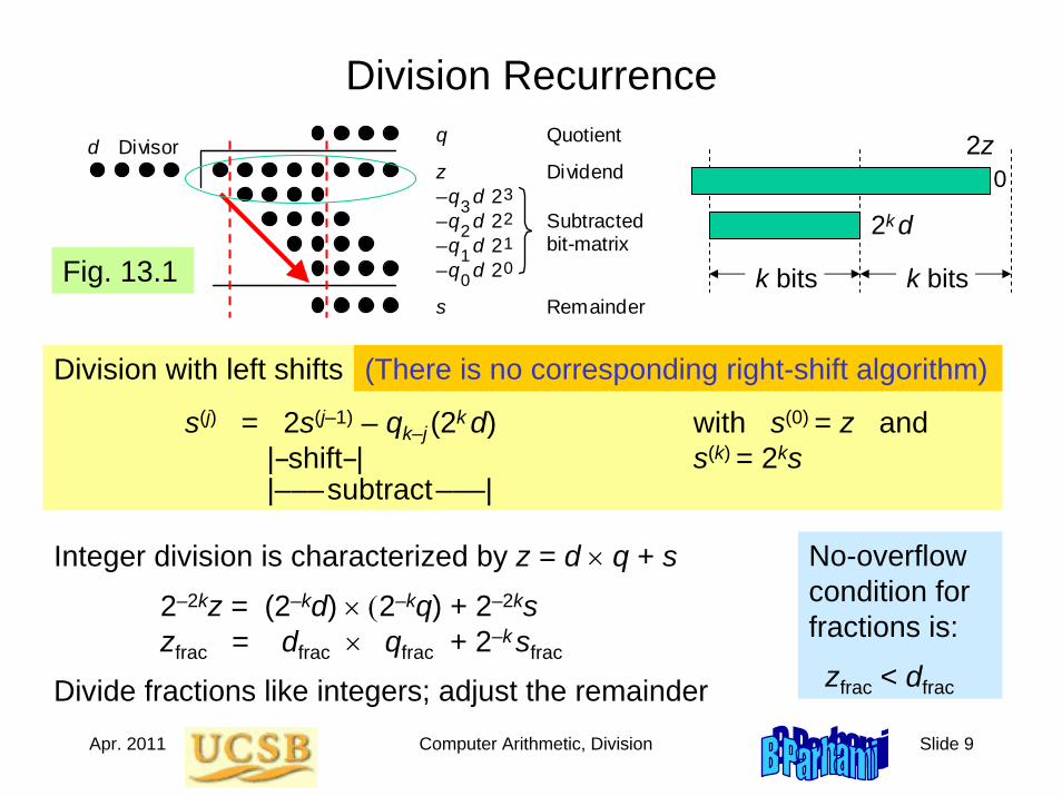
Division Recurrence
Division with left shifts
s(j) = 2s(j–1) – qk–j (2k d) with s(0) = z and|–shift–| s(k) = 2ks|–––subtract–––|
(There is no corresponding right-shift algorithm)
Fig. 13.1
Dividend
Subtracted bit-matrix
z
s Remainder
Quotient q Divisor d
q d 2 3 3 –
q d 2 2 2 –
q d 2 1 1 –
q d 2 0 0 –
Integer division is characterized by z = d × q + s
2–2kz = (2–kd) × (2–kq) + 2–2kszfrac = dfrac × qfrac + 2–ksfrac
Divide fractions like integers; adjust the remainder
No-overflow condition for fractions is:
zfrac < dfrac
k bits k bits
2z
2k d
0
Apr. 2011 Computer Arithmetic, Division Slide 10
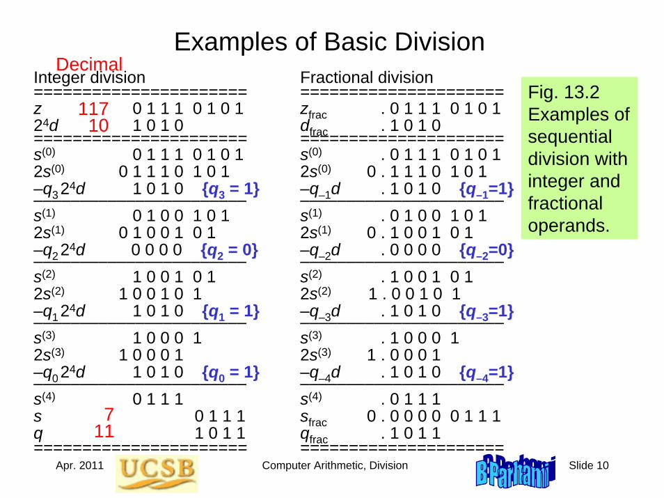
Examples of Basic Division
Fig. 13.2 Examples of sequential division with integer and fractional operands.
Integer division Fractional division====================== =====================z 0 1 1 1 0 1 0 1 zfrac . 0 1 1 1 0 1 0 124d 1 0 1 0 dfrac . 1 0 1 0 ====================== =====================s(0) 0 1 1 1 0 1 0 1 s(0) . 0 1 1 1 0 1 0 12s(0) 0 1 1 1 0 1 0 1 2s(0) 0 . 1 1 1 0 1 0 1–q3 24d 1 0 1 0 {q3 = 1} –q–1d . 1 0 1 0 {q–1=1}––––––––––––––––––––––– ––––––––––––––––––––––s(1) 0 1 0 0 1 0 1 s(1) . 0 1 0 0 1 0 12s(1) 0 1 0 0 1 0 1 2s(1) 0 . 1 0 0 1 0 1–q2 24d 0 0 0 0 {q2 = 0} –q–2d . 0 0 0 0 {q–2=0}––––––––––––––––––––––– ––––––––––––––––––––––s(2) 1 0 0 1 0 1 s(2) . 1 0 0 1 0 12s(2) 1 0 0 1 0 1 2s(2) 1 . 0 0 1 0 1–q1 24d 1 0 1 0 {q1 = 1} –q–3d . 1 0 1 0 {q–3=1}––––––––––––––––––––––– ––––––––––––––––––––––s(3) 1 0 0 0 1 s(3) . 1 0 0 0 12s(3) 1 0 0 0 1 2s(3) 1 . 0 0 0 1–q0 24d 1 0 1 0 {q0 = 1} –q–4d . 1 0 1 0 {q–4=1}––––––––––––––––––––––– ––––––––––––––––––––––s(4) 0 1 1 1 s(4) . 0 1 1 1s 0 1 1 1 sfrac 0 . 0 0 0 0 0 1 1 1q 1 0 1 1 qfrac . 1 0 1 1====================== =====================
10
117
117
Decimal
Apr. 2011 Computer Arithmetic, Division Slide 11
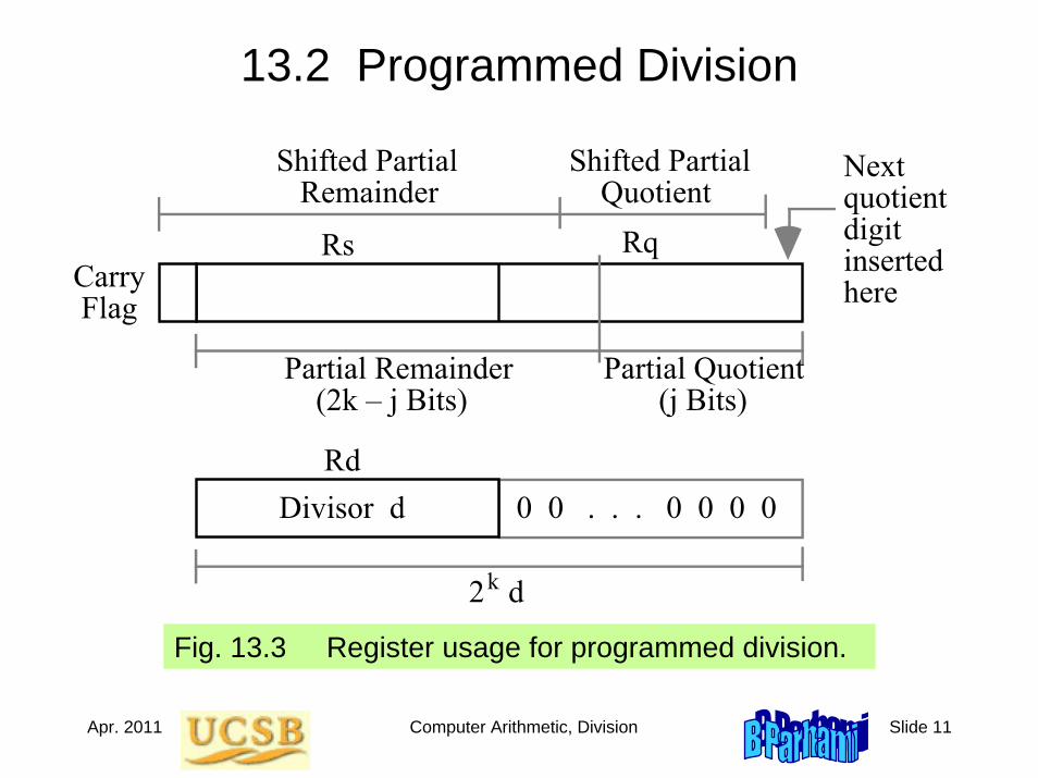
13.2 Programmed Division
Fig. 13.3 Register usage for programmed division.
Rs Rq
Rd0 0 . . . 0 0 0 0
2 dk
Carry Flag
Shifted Partial Remainder
Shifted Partial Quotient
Partial Remainder (2k – j Bits)
Partial Quotient (j Bits)
Next quotient digit inserted here
Divisor d
Apr. 2011 Computer Arithmetic, Division Slide 12
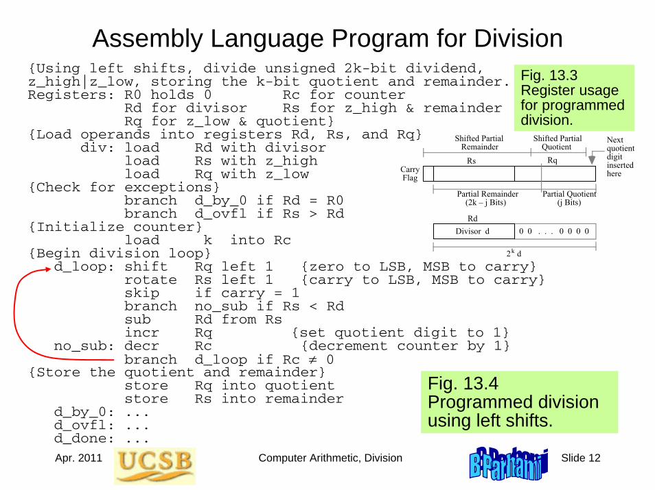
Assembly Language Program for Division
Fig. 13.4Programmed division using left shifts.
{Using left shifts, divide unsigned 2k-bit dividend,z_high|z_low, storing the k-bit quotient and remainder. Registers: R0 holds 0 Rc for counter
Rd for divisor Rs for z_high & remainder Rq for z_low & quotient}
{Load operands into registers Rd, Rs, and Rq}div: load Rd with divisor
load Rs with z_highload Rq with z_low
{Check for exceptions} branch d_by_0 if Rd = R0branch d_ovfl if Rs > Rd
{Initialize counter}load k into Rc
{Begin division loop}d_loop: shift Rq left 1 {zero to LSB, MSB to carry}
rotate Rs left 1 {carry to LSB, MSB to carry}skip if carry = 1branch no_sub if Rs < Rd sub Rd from Rs incr Rq {set quotient digit to 1}
no_sub: decr Rc {decrement counter by 1}branch d_loop if Rc ≠ 0
{Store the quotient and remainder}store Rq into quotientstore Rs into remainder
d_by_0: ...d_ovfl: ...d_done: ...
Rs Rq
Rd0 0 . . . 0 0 0 0
2 dk
Carry Flag
Shifted Partial Remainder
Shifted Partial Quotient
Partial Remainder (2k – j Bits)
Partial Quotient (j Bits)
Next quotient digit inserted here
Divisor d
Fig. 13.3 Register usage for programmed division.

Apr. 2011 Computer Arithmetic, Division Slide 13
Time Complexity of Programmed Division
Assume k-bit words
k iterations of the main loop 6-8 instructions per iteration, depending on the quotient bit
Thus, 6k + 3 to 8k + 3 machine instructions,ignoring operand loads and result store
k = 32 implies 220+ instructions on average
This is too slow for many modern applications!
Microprogrammed division would be somewhat better
Apr. 2011 Computer Arithmetic, Division Slide 14
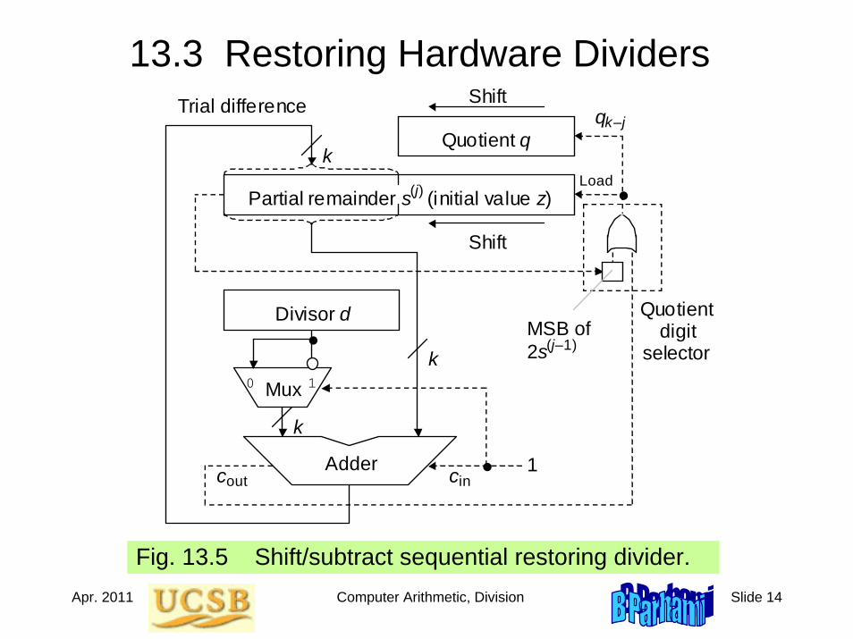
13.3 Restoring Hardware Dividers
Fig. 13.5 Shift/subtract sequential restoring divider.
Quotient q
Mux
Adder out c
0 1
Partial remainder s (initial value z)
Divisor d
Shift
Shift
Load
1 in c
(j)
Quotient digit
selector
q k–j
MSB of 2s (j–1)
k
k
k
Trial difference
Apr. 2011 Computer Arithmetic, Division Slide 15
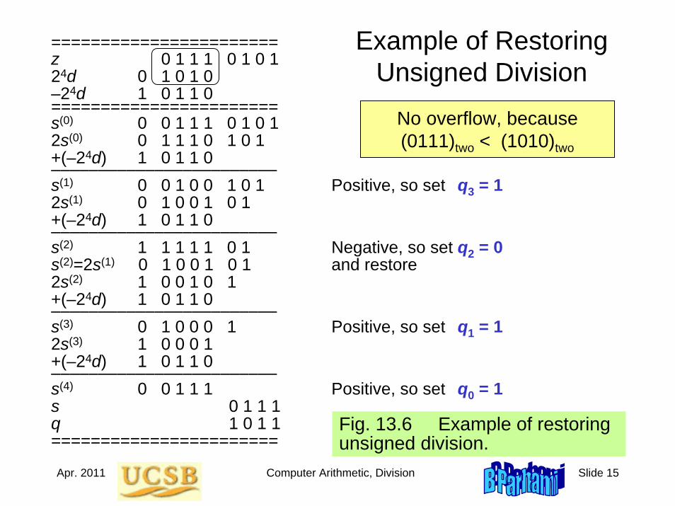
Example of Restoring Unsigned Division
Fig. 13.6 Example of restoring unsigned division.
=======================z 0 1 1 1 0 1 0 124d 0 1 0 1 0–24d 1 0 1 1 0=======================s(0) 0 0 1 1 1 0 1 0 1 2s(0) 0 1 1 1 0 1 0 1 +(–24d) 1 0 1 1 0 ––––––––––––––––––––––––s(1) 0 0 1 0 0 1 0 1 Positive, so set q3 = 12s(1) 0 1 0 0 1 0 1 +(–24d) 1 0 1 1 0 ––––––––––––––––––––––––s(2) 1 1 1 1 1 0 1 Negative, so set q2 = 0s(2)=2s(1) 0 1 0 0 1 0 1 and restore2s(2) 1 0 0 1 0 1 +(–24d) 1 0 1 1 0 ––––––––––––––––––––––––s(3) 0 1 0 0 0 1 Positive, so set q1 = 12s(3) 1 0 0 0 1 +(–24d) 1 0 1 1 0 ––––––––––––––––––––––––s(4) 0 0 1 1 1 Positive, so set q0 = 1s 0 1 1 1 q 1 0 1 1=======================
No overflow, because(0111)two < (1010)two
Apr. 2011 Computer Arithmetic, Division Slide 16
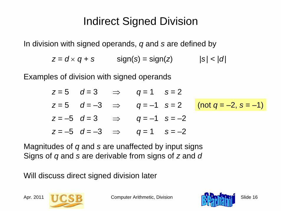
Indirect Signed Division
In division with signed operands, q and s are defined by
z = d × q + s sign(s) = sign(z) |s | < |d |
Examples of division with signed operands
z = 5 d = 3 ⇒ q = 1 s = 2
z = 5 d = –3 ⇒ q = –1 s = 2
z = –5 d = 3 ⇒ q = –1 s = –2
z = –5 d = –3 ⇒ q = 1 s = –2
Magnitudes of q and s are unaffected by input signsSigns of q and s are derivable from signs of z and d
Will discuss direct signed division later
(not q = –2, s = –1)
Apr. 2011 Computer Arithmetic, Division Slide 17
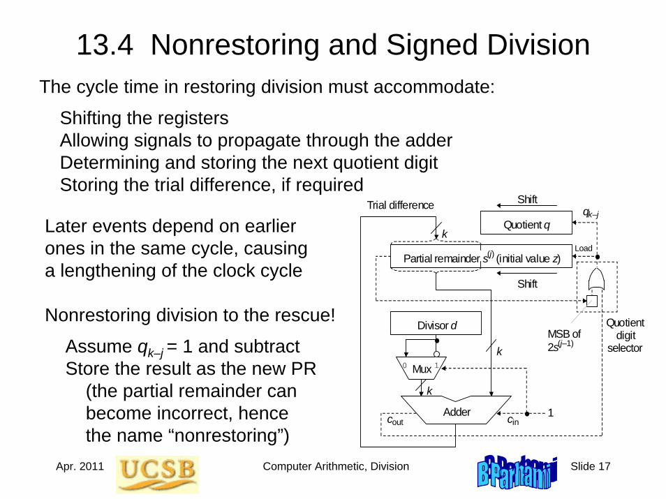
13.4 Nonrestoring and Signed DivisionThe cycle time in restoring division must accommodate:
Shifting the registersAllowing signals to propagate through the adderDetermining and storing the next quotient digitStoring the trial difference, if required
Quotient q
Mux
Adder out c
0 1
Partial remainder s (initial value z)
Divisor d
Shift
Shift
Load
1 in c
(j)
Quotient digit
selector
q k–j
MSB of 2s (j–1)
k
k
k
Trial difference
Later events depend on earlier ones in the same cycle, causing a lengthening of the clock cycle
Nonrestoring division to the rescue!
Assume qk–j = 1 and subtractStore the result as the new PR
(the partial remainder can become incorrect, hencethe name “nonrestoring”)
Apr. 2011 Computer Arithmetic, Division Slide 18
Justification for Nonrestoring Division
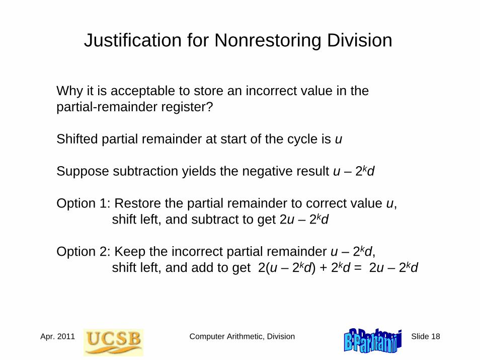
Why it is acceptable to store an incorrect value in the partial-remainder register?
Shifted partial remainder at start of the cycle is u
Suppose subtraction yields the negative result u – 2kd
Option 1: Restore the partial remainder to correct value u, shift left, and subtract to get 2u – 2kd
Option 2: Keep the incorrect partial remainder u – 2kd, shift left, and add to get 2(u – 2kd) + 2kd = 2u – 2kd
Apr. 2011 Computer Arithmetic, Division Slide 19
Example of Nonrestoring Unsigned Division
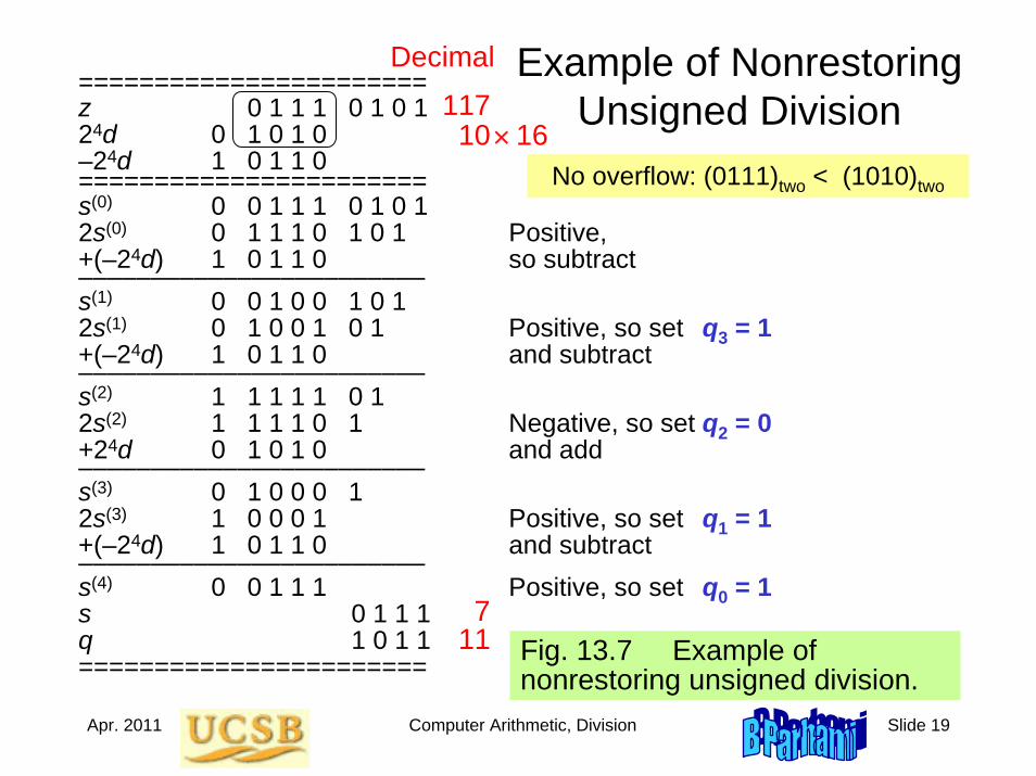
Fig. 13.7 Example of nonrestoring unsigned division.
=======================z 0 1 1 1 0 1 0 124d 0 1 0 1 0–24d 1 0 1 1 0=======================s(0) 0 0 1 1 1 0 1 0 1 2s(0) 0 1 1 1 0 1 0 1 Positive,+(–24d) 1 0 1 1 0 so subtract––––––––––––––––––––––––s(1) 0 0 1 0 0 1 0 1 2s(1) 0 1 0 0 1 0 1 Positive, so set q3 = 1+(–24d) 1 0 1 1 0 and subtract––––––––––––––––––––––––s(2) 1 1 1 1 1 0 1 2s(2) 1 1 1 1 0 1 Negative, so set q2 = 0+24d 0 1 0 1 0 and add––––––––––––––––––––––––s(3) 0 1 0 0 0 1 2s(3) 1 0 0 0 1 Positive, so set q1 = 1+(–24d) 1 0 1 1 0 and subtract––––––––––––––––––––––––s(4) 0 0 1 1 1 Positive, so set q0 = 1s 0 1 1 1 q 1 0 1 1=======================
No overflow: (0111)two < (1010)two
10 × 16
117
117
Decimal
Apr. 2011 Computer Arithmetic, Division Slide 20
Graphical Depiction of Nonrestoring Division
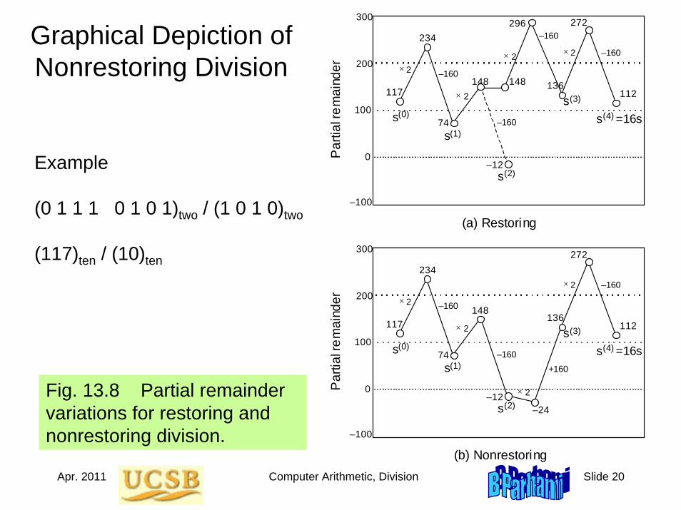
Fig. 13.8 Partial remainder variations for restoring and nonrestoring division.
300
200
100
0
–100
117
234
74
148
–12
296
136
272
112
s
(0)
s
(1)
s
(2)
s
(3) s =16s
(4)
–160
2
×
2
×
2
×
×
2
–160
–160 –160
Par
tial r
emai
nder
(a) Restoring
148
300
200
100
0
–100
117
234
74
148
–12 –24
136
272
112
s
(0)
s
(1)
s
(2)
s
(3) s =16s
(4)
–160
2
×
2
×
2
×
×
2
–160 +160
–160
Par
tial r
emai
nder
(b) Nonrestoring
Example
(0 1 1 1 0 1 0 1)two / (1 0 1 0)two
(117)ten / (10)ten
Apr. 2011 Computer Arithmetic, Division Slide 21
Convergence of the Partial Quotient to q
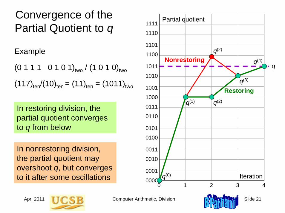
In restoring division, the partial quotient converges to q from below
Example
(0 1 1 1 0 1 0 1)two / (1 0 1 0)two
(117)ten/(10)ten = (11)ten = (1011)two
In nonrestoring division, the partial quotient may overshoot q, but converges to it after some oscillations 0000
0001
0010
0011
0100
0101
0110
0111
1000
1001
1010
1011
1100
1101
1110
1111Partial quotient
Iteration0 1 2 3 4
q
q(1) q(2)
q(3)
q(4)
q(2)
Restoring
Nonrestoring
q(0)
Apr. 2011 Computer Arithmetic, Division Slide 22
Nonrestoring Division with Signed Operands
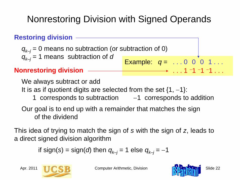
Restoring divisionqk–j = 0 means no subtraction (or subtraction of 0)qk–j = 1 means subtraction of d
Nonrestoring divisionWe always subtract or addIt is as if quotient digits are selected from the set {1, −1}:
1 corresponds to subtraction −1 corresponds to addition
Our goal is to end up with a remainder that matches the signof the dividend
This idea of trying to match the sign of s with the sign of z, leads to a direct signed division algorithm
if sign(s) = sign(d) then qk–j = 1 else qk–j = −1
Example: q = . . . 0 0 0 1 . . .. . . 1 −1 −1 −1 . . .
Apr. 2011 Computer Arithmetic, Division Slide 23
Quotient Conversion and Final Correction
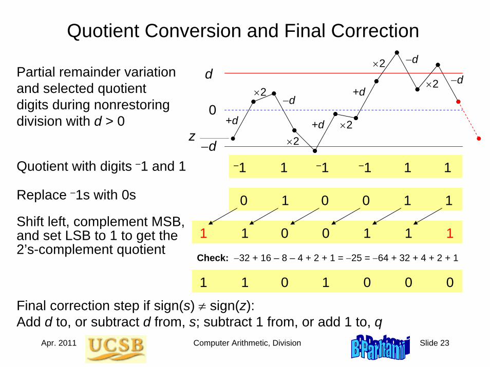
Partial remainder variation and selected quotient digits during nonrestoring division with d > 0
d
0
−d
+d
−d
−d
−d
+d
+d
×2×2
×2
×2×2
−1 1 −1 −1 1 1
z
0 1 0 0 1 1
1 1 0 0 1 1 1
Quotient with digits −1 and 1
Check: −32 + 16 – 8 – 4 + 2 + 1 = −25 = −64 + 32 + 4 + 2 + 1
Replace −1s with 0s
Final correction step if sign(s) ≠ sign(z):Add d to, or subtract d from, s; subtract 1 from, or add 1 to, q
Shift left, complement MSB, and set LSB to 1 to get the 2’s-complement quotient
1 1 0 1 0 0 0
Apr. 2011 Computer Arithmetic, Division Slide 24
Example of Nonrestoring Signed Division
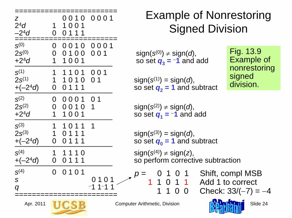
Fig. 13.9 Example of nonrestoring signed division.
========================z 0 0 1 0 0 0 0 124d 1 1 0 0 1–24d 0 0 1 1 1========================s(0) 0 0 0 1 0 0 0 0 1 2s(0) 0 0 1 0 0 0 0 1 sign(s(0)) ≠ sign(d),+24d 1 1 0 0 1 so set q3 = −1 and add––––––––––––––––––––––––s(1) 1 1 1 0 1 0 0 1 2s(1) 1 1 0 1 0 0 1 sign(s(1)) = sign(d), +(–24d) 0 0 1 1 1 so set q2 = 1 and subtract––––––––––––––––––––––––s(2) 0 0 0 0 1 0 1 2s(2) 0 0 0 1 0 1 sign(s(2)) ≠ sign(d),+24d 1 1 0 0 1 so set q1 = −1 and add––––––––––––––––––––––––s(3) 1 1 0 1 1 1 2s(3) 1 0 1 1 1 sign(s(3)) = sign(d), +(–24d) 0 0 1 1 1 so set q0 = 1 and subtract––––––––––––––––––––––––s(4) 1 1 1 1 0 sign(s(4)) ≠ sign(z),+(–24d) 0 0 1 1 1 so perform corrective subtraction––––––––––––––––––––––––s(4) 0 0 1 0 1 s 0 1 0 1 q −1 1−1 1========================
p = 0 1 0 1 Shift, compl MSB1 1 0 1 1 Add 1 to correct
1 1 0 0 Check: 33/(−7) = −4
Apr. 2011 Computer Arithmetic, Division Slide 25
Nonrestoring Hardware Divider
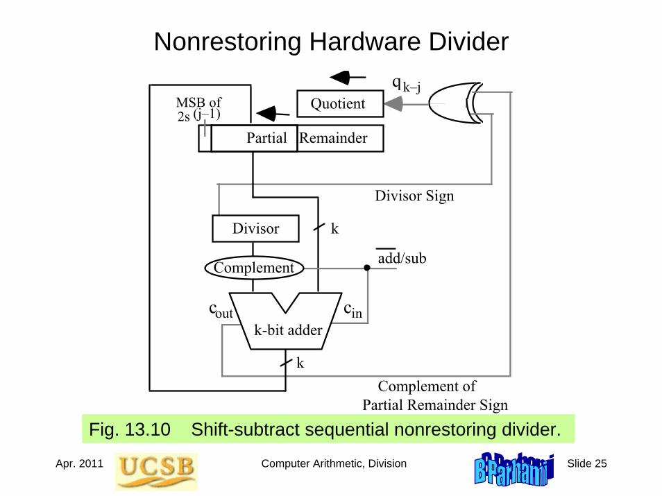
Fig. 13.10 Shift-subtract sequential nonrestoring divider.
Quotient
k
Partial Remainder
Divisor
add/sub
k-bit adder
k
cout cin
Complement
qk–j 2s (j–1)MSB of
Divisor Sign
Complement of Partial Remainder Sign

Apr. 2011 Computer Arithmetic, Division Slide 26
13.5 Division by ConstantsSoftware and hardware aspects:As was the case for multiplications by constants, optimizing compilers may replace some divisions by shifts/adds/subs; likewise, in custom VLSI circuits, hardware dividers may be replaced by simpler adders
Method 1: Find the reciprocal of the constant and multiply (particularly efficient if several numbers must be divided by the same divisor)
Method 2: Use the property that for each odd integer d, there exists an odd integer m such that d × m = 2n – 1; hence, d = (2n – 1)/m and
Number of shift-adds required is proportional to log k
Multiplication by constant Shift-adds
L)21)(21)(21(2)21(212
42 nnnnnnn
zmzmzmdz −−−
− +++=−
=−
=
Apr. 2011 Computer Arithmetic, Division Slide 27
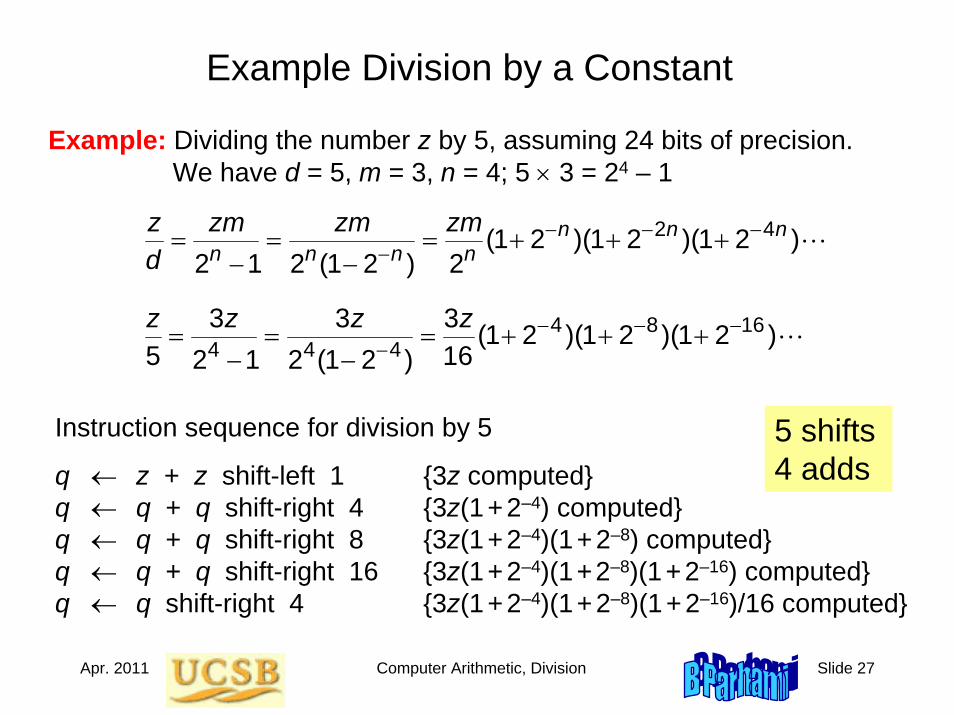
Example Division by a Constant
L)21)(21)(21(2)21(212
42 nnnnnnn
zmzmzmdz −−−
− +++=−
=−
=
Example: Dividing the number z by 5, assuming 24 bits of precision. We have d = 5, m = 3, n = 4; 5 × 3 = 24 – 1
Instruction sequence for division by 5
q ← z + z shift-left 1 {3z computed}q ← q + q shift-right 4 {3z(1+2–4) computed}q ← q + q shift-right 8 {3z(1+2–4)(1+2–8) computed}q ← q + q shift-right 16 {3z(1+2–4)(1+2–8)(1+2–16) computed}q ← q shift-right 4 {3z(1+2–4)(1+2–8)(1+2–16)/16 computed}
L)21)(21)(21(163
)21(23
123
51684
444−−−
− +++=−
=−
=zzzz
5 shifts4 adds
Apr. 2011 Computer Arithmetic, Division Slide 28
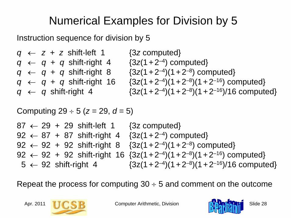
Numerical Examples for Division by 5Instruction sequence for division by 5
q ← z + z shift-left 1 {3z computed}q ← q + q shift-right 4 {3z(1+2–4) computed}q ← q + q shift-right 8 {3z(1+2–4)(1+2–8) computed}q ← q + q shift-right 16 {3z(1+2–4)(1+2–8)(1+2–16) computed}q ← q shift-right 4 {3z(1+2–4)(1+2–8)(1+2–16)/16 computed}
Computing 29 ÷ 5 (z = 29, d = 5)
87 ← 29 + 29 shift-left 1 {3z computed}92 ← 87 + 87 shift-right 4 {3z(1+2–4) computed}92 ← 92 + 92 shift-right 8 {3z(1+2–4)(1+2–8) computed}92 ← 92 + 92 shift-right 16 {3z(1+2–4)(1+2–8)(1+2–16) computed}5 ← 92 shift-right 4 {3z(1+2–4)(1+2–8)(1+2–16)/16 computed}
Repeat the process for computing 30 ÷ 5 and comment on the outcome
Apr. 2011 Computer Arithmetic, Division Slide 29
13.6 Radix-2 SRT Division
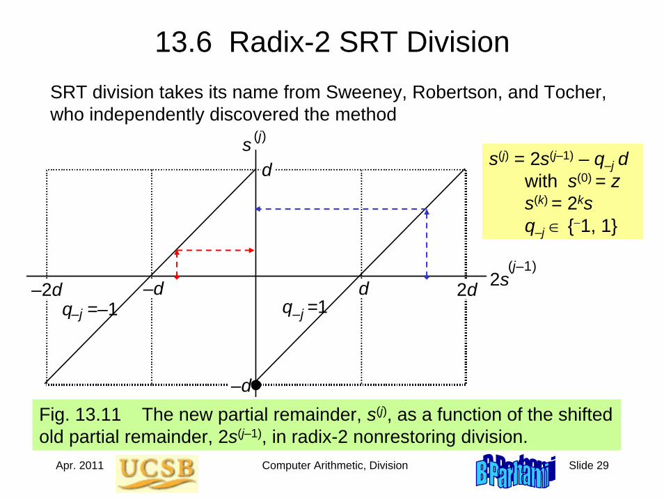
Fig. 13.11 The new partial remainder, s(j), as a function of the shifted old partial remainder, 2s(j–1), in radix-2 nonrestoring division.
SRT division takes its name from Sweeney, Robertson, and Tocher, who independently discovered the method
–2d
2d
d
–d
q =–1
q =1
2s
(j–1)
s
(j)
–j
–j
d
–d
s(j) = 2s(j–1) – q–j dwith s(0) = zs(k) = 2ksq–j ∈ {−1, 1}
Apr. 2011 Computer Arithmetic, Division Slide 30
–2d
2d
d
–d
q =–1
q =0
q =1
2s
(j–1)
s
(j)
–j
–j
–j
d
–d
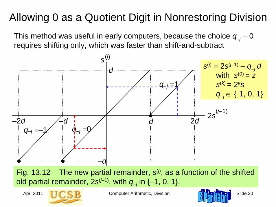
Allowing 0 as a Quotient Digit in Nonrestoring Division
Fig. 13.12 The new partial remainder, s(j), as a function of the shifted old partial remainder, 2s(j–1), with q–j in {−1, 0, 1}.
This method was useful in early computers, because the choice q–j = 0 requires shifting only, which was faster than shift-and-subtract
s(j) = 2s(j–1) – q–j dwith s(0) = zs(k) = 2ksq–j ∈ {−1, 0, 1}
Apr. 2011 Computer Arithmetic, Division Slide 31
–2d
2d
d
–d
q =–1
q =0
q =1
2s
(j–1)
s
(j)
–j
–j
–j
d
–d
–1/2 1/2
–1
1
–1/2
1/2
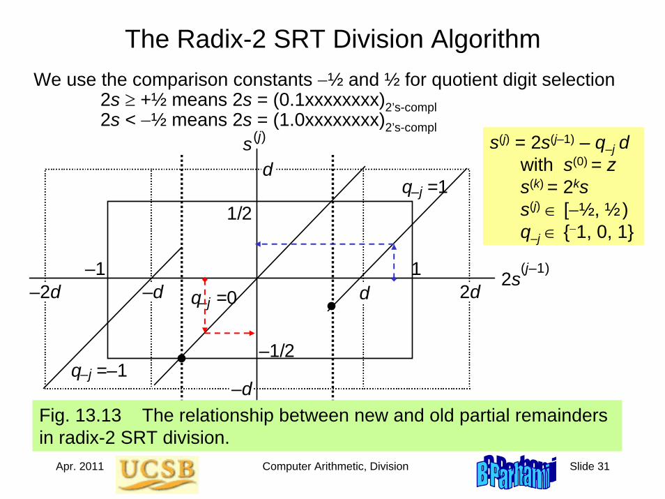
The Radix-2 SRT Division Algorithm
Fig. 13.13 The relationship between new and old partial remainders in radix-2 SRT division.
We use the comparison constants −½ and ½ for quotient digit selection2s ≥ +½ means 2s = (0.1xxxxxxxx)2’s-compl2s < −½ means 2s = (1.0xxxxxxxx)2’s-compl
s(j) = 2s(j–1) – q–j dwith s(0) = zs(k) = 2kss(j) ∈ [−½, ½)q–j ∈ {−1, 0, 1}
Apr. 2011 Computer Arithmetic, Division Slide 32
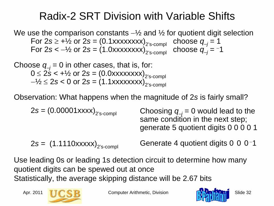
Radix-2 SRT Division with Variable ShiftsWe use the comparison constants −½ and ½ for quotient digit selection
For 2s ≥ +½ or 2s = (0.1xxxxxxxx)2’s-compl choose q–j = 1For 2s < −½ or 2s = (1.0xxxxxxxx)2’s-compl choose q–j = −1
Choose q–j = 0 in other cases, that is, for:0 ≤ 2s < +½ or 2s = (0.0xxxxxxxx)2’s-compl−½ ≤ 2s < 0 or 2s = (1.1xxxxxxxx)2’s-compl
Observation: What happens when the magnitude of 2s is fairly small?
2s = (0.00001xxxx)2’s-compl
2s = (1.1110xxxxx)2’s-compl
Choosing q–j = 0 would lead to the same condition in the next step; generate 5 quotient digits 0 0 0 0 1
Generate 4 quotient digits 0 0 0 −1
Use leading 0s or leading 1s detection circuit to determine how many quotient digits can be spewed out at onceStatistically, the average skipping distance will be 2.67 bits
Apr. 2011 Computer Arithmetic, Division Slide 33
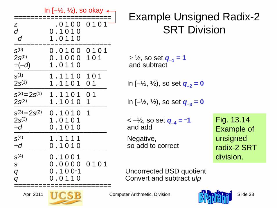
Example Unsigned Radix-2 SRT Division
Fig. 13.14 Example of unsigned radix-2 SRT division.
========================z . 0 1 0 0 0 1 0 1d 0 . 1 0 1 0–d 1 . 0 1 1 0========================s(0) 0 . 0 1 0 0 0 1 0 1 2s(0) 0 . 1 0 0 0 1 0 1 ≥ ½, so set q−1 = 1+(−d) 1 . 0 1 1 0 and subtract––––––––––––––––––––––––s(1) 1 . 1 1 1 0 1 0 1 2s(1) 1 . 1 1 0 1 0 1 In [−½, ½), so set q−2 = 0––––––––––––––––––––––––s(2) =2s(1) 1 . 1 1 0 1 0 1 2s(2) 1 . 1 0 1 0 1 In [−½, ½), so set q−3 = 0––––––––––––––––––––––––s(3) =2s(2) 0 . 1 0 1 0 1 2s(3) 1 . 0 1 0 1 < −½, so set q−4 = −1+d 0 . 1 0 1 0 and add––––––––––––––––––––––––s(4) 1 . 1 1 1 1 Negative,+d 0 . 1 0 1 0 so add to correct––––––––––––––––––––––––s(4) 0 . 1 0 0 1 s 0 . 0 0 0 0 0 1 0 1 q 0 . 1 0 0−1 Uncorrected BSD quotientq 0 . 0 1 1 0 Convert and subtract ulp========================
In [−½, ½), so okay
Apr. 2011 Computer Arithmetic, Division Slide 34
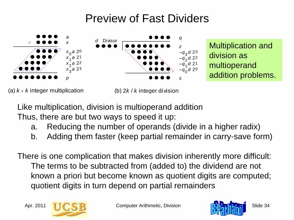
Preview of Fast Dividers
Like multiplication, division is multioperand addition Thus, there are but two ways to speed it up:
a. Reducing the number of operands (divide in a higher radix)b. Adding them faster (keep partial remainder in carry-save form)
a x
p
2
x a
0 0
1 x a 2 1 x a 2
2 2
2 3 3
x a
×
(a) k × k integer multiplication
z
s
q Divisor d
q d 2 3 3 –
q d 2 2 2 –
q d 2 1 1 –
q d 2 0 0 –
(b) 2k / k integer division
Multiplication and division as multioperand addition problems.
There is one complication that makes division inherently more difficult: The terms to be subtracted from (added to) the dividend are not known a priori but become known as quotient digits are computed;quotient digits in turn depend on partial remainders
Apr. 2011 Computer Arithmetic, Division Slide 35
14 High-Radix DividersChapter Goals
Study techniques that allow us to obtainmore than one quotient bit in each cycle(two bits in radix 4, three in radix 8, . . .)
Chapter HighlightsRadix > 2 ⇒ quotient digit selection harder Remedy: redundant quotient representationCarry-save addition reduces cycle timeQuotient digit selectionImplementation methods and tradeoffs
Apr. 2011 Computer Arithmetic, Division Slide 36
High-Radix Dividers: Topics
Topics in This Chapter
14.1 Basics of High-Radix Division
14.2 Using Carry-Save Adders
14.3 Radix-4 SRT Division
14.4 General High-Radix Dividers
14.5 Quotient Digit Selection
14.6 Using p-d Plots in Practice
Apr. 2011 Computer Arithmetic, Division Slide 37
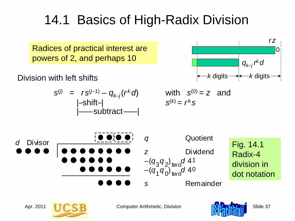
14.1 Basics of High-Radix Division
Division with left shifts
s(j) = rs(j–1) – qk–j (r k d) with s(0) = z and|–shift–| s(k) = r ks|–––subtract–––|
Radices of practical interest are powers of 2, and perhaps 10
Dividend z
s Remainder
Quotient q Divisor d
(q q ) d 4 1 3 – 2 two
4 0 d (q q ) 1 – 0 two
Fig. 14.1 Radix-4 division in dot notation
k digits k digits
rz
qk–j rk d
0
Apr. 2011 Computer Arithmetic, Division Slide 38
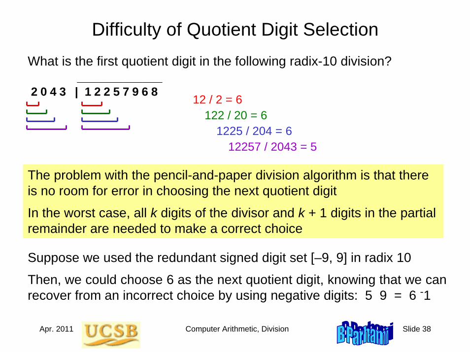
Difficulty of Quotient Digit SelectionWhat is the first quotient digit in the following radix-10 division?
_____________2 0 4 3 | 1 2 2 5 7 9 6 8
The problem with the pencil-and-paper division algorithm is that there is no room for error in choosing the next quotient digit
In the worst case, all k digits of the divisor and k + 1 digits in the partial remainder are needed to make a correct choice
12 / 2 = 6122 / 20 = 6
1225 / 204 = 612257 / 2043 = 5
Suppose we used the redundant signed digit set [–9, 9] in radix 10
Then, we could choose 6 as the next quotient digit, knowing that we canrecover from an incorrect choice by using negative digits: 5 9 = 6 -1
Apr. 2011 Computer Arithmetic, Division Slide 39
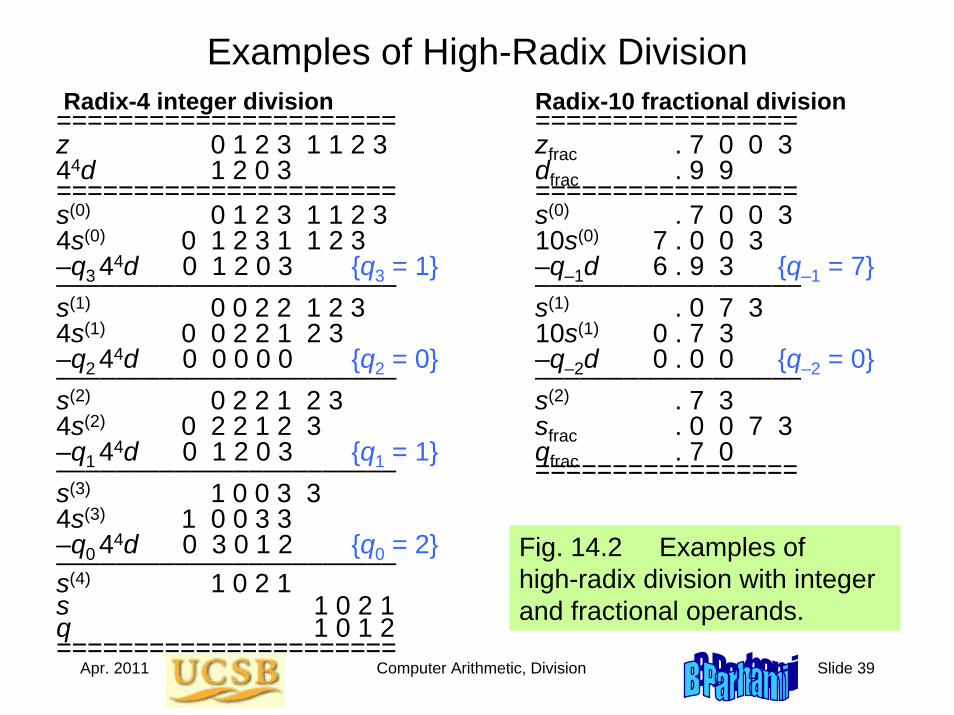
Examples of High-Radix DivisionRadix-4 integer division Radix-10 fractional division====================== =================z 0 1 2 3 1 1 2 3 zfrac . 7 0 0 3 44d 1 2 0 3 dfrac . 9 9 ====================== =================s(0) 0 1 2 3 1 1 2 3 s(0) . 7 0 0 34s(0) 0 1 2 3 1 1 2 3 10s(0) 7 . 0 0 3–q3 44d 0 1 2 0 3 {q3 = 1} –q–1d 6 . 9 3 {q–1 = 7}––––––––––––––––––––––– ––––––––––––––––––s(1) 0 0 2 2 1 2 3 s(1) . 0 7 34s(1) 0 0 2 2 1 2 3 10s(1) 0 . 7 3–q2 44d 0 0 0 0 0 {q2 = 0} –q–2d 0 . 0 0 {q–2 = 0}––––––––––––––––––––––– ––––––––––––––––––s(2) 0 2 2 1 2 3 s(2) . 7 34s(2) 0 2 2 1 2 3 sfrac . 0 0 7 3–q1 44d 0 1 2 0 3 {q1 = 1} qfrac . 7 0––––––––––––––––––––––– =================s(3) 1 0 0 3 3 4s(3) 1 0 0 3 3 –q0 44d 0 3 0 1 2 {q0 = 2}–––––––––––––––––––––––s(4) 1 0 2 1 s 1 0 2 1 q 1 0 1 2======================
Fig. 14.2 Examples of high-radix division with integer and fractional operands.
Apr. 2011 Computer Arithmetic, Division Slide 40
14.2 Using Carry-Save Adders
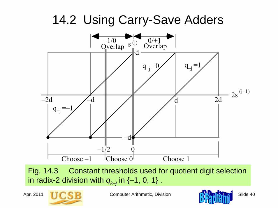
Fig. 14.3 Constant thresholds used for quotient digit selection in radix-2 division with qk–j in {–1, 0, 1} .
–2d 2d
d
–d
q =–1
q =0 q =1
2s (j–1)
s (j)
–j
–j
–j
d–d
–1/2 0Choose –1 Choose 0 Choose 1
–1/0 0/+1Overlap Overlap
Apr. 2011 Computer Arithmetic, Division Slide 41
Quotient Digit Selection Based on Truncated PR
Fig. 14.3
–2d 2d
d
–d
q =–1
q =0 q =1
2s (j–1)
s (j)
–j
–j
–j
d–d
–1/2 0Choose –1 Choose 0 Choose 1
–1/0 0/+1Overlap Overlap
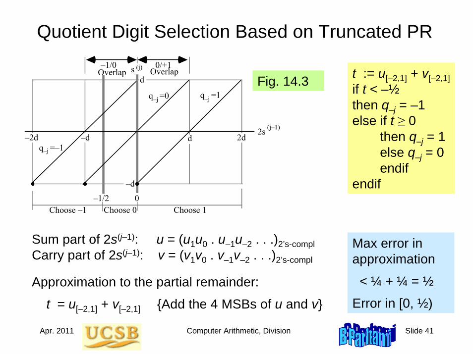
Sum part of 2s(j–1): u = (u1u0 . u–1u–2 . . .)2’s-complCarry part of 2s(j–1): v = (v1v0 . v–1v–2 . . .)2’s-compl
Approximation to the partial remainder:
t = u[–2,1] + v[–2,1] {Add the 4 MSBs of u and v}
t := u[–2,1] + v[–2,1]if t < –½then q–j = –1else if t ≥ 0
then q–j = 1else q–j = 0endif
endif
Max error in approximation
< ¼ + ¼ = ½
Error in [0, ½)
Apr. 2011 Computer Arithmetic, Division Slide 42
Divider with Partial Remainder in Carry-Save Form
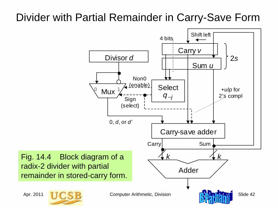
Fig. 14.4 Block diagram of a radix-2 divider with partial remainder in stored-carry form.
Carry v
Mux
Adder
0 1
Divisor d
k k
Carry-save adder
Select q –j
4 bits Shift left
2s
+ulp for 2’s compl
Sum u
Non0 (enable)
Sign (select)
0, d, or d’
Carry Sum
Apr. 2011 Computer Arithmetic, Division Slide 43
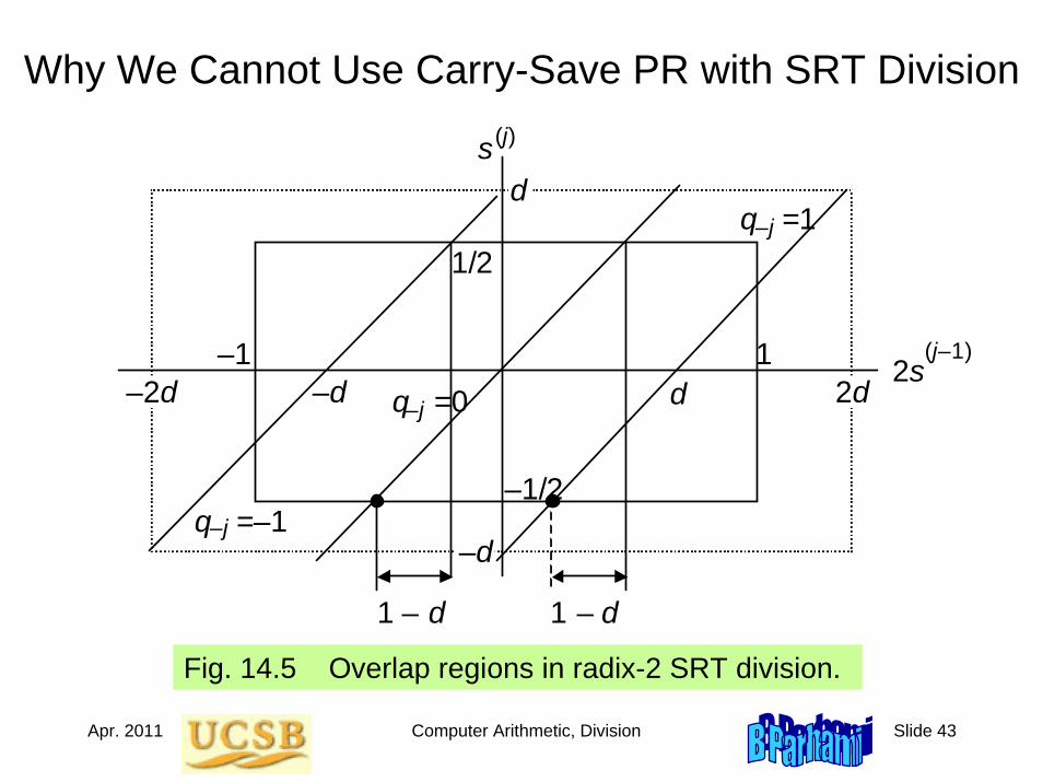
Why We Cannot Use Carry-Save PR with SRT Division
Fig. 14.5 Overlap regions in radix-2 SRT division.
–2d
2d
d
–d
q =–1
q =0
q =1
2s
(j–1)
s
(j)
–j
–j
–j
d
–d
1 – d
–1
1
–1/2
1/2
1 – d
Apr. 2011 Computer Arithmetic, Division Slide 44
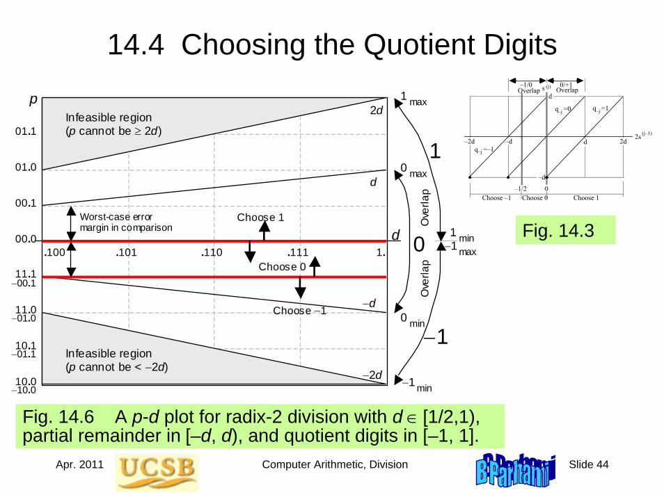
14.4 Choosing the Quotient Digits
Fig. 14.6 A p-d plot for radix-2 division with d ∈ [1/2,1), partial remainder in [–d, d), and quotient digits in [–1, 1].
d
p
Infeasible region (p cannot be ≥ 2d)
Infeasible region (p cannot be < −2d)
.100 .101 .110 .111 1.
00.1
00.0
11.1
10.0
10.1
11.0
01.1
01.0
−00.1
−01.0
−01.1
−10.0
d
2d
−2d
−d
Worst-case error margin in comparison
Choose 1
Choose −1
Choose 0
−1
1
−1 max
−1 min
1 min
1 max
0 max
0 min
Ove
rlap
Ove
rlap
0 Fig. 14.3
–2d 2d
d
–d
q =–1
q =0 q =1
2s (j–1)
s (j)
–j
–j
–j
d–d
–1/2 0Choose –1 Choose 0 Choose 1
–1/0 0/+1Overlap Overlap
Apr. 2011 Computer Arithmetic, Division Slide 45
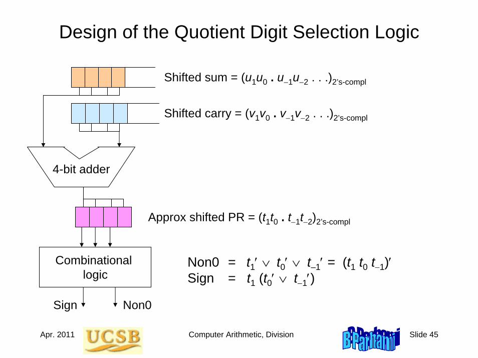
Design of the Quotient Digit Selection Logic
4-bit adder
Combinational logic
Non0Sign
Shifted sum = (u1u0 . u−1u−2 . . .)2’s-compl
Shifted carry = (v1v0 . v−1v−2 . . .)2’s-compl
Approx shifted PR = (t1t0 . t−1t−2)2’s-compl
Non0 = t1′ ∨ t0′ ∨ t–1′ = (t1 t0 t−1)′Sign = t1 (t0′ ∨ t−1′)
Apr. 2011 Computer Arithmetic, Division Slide 46
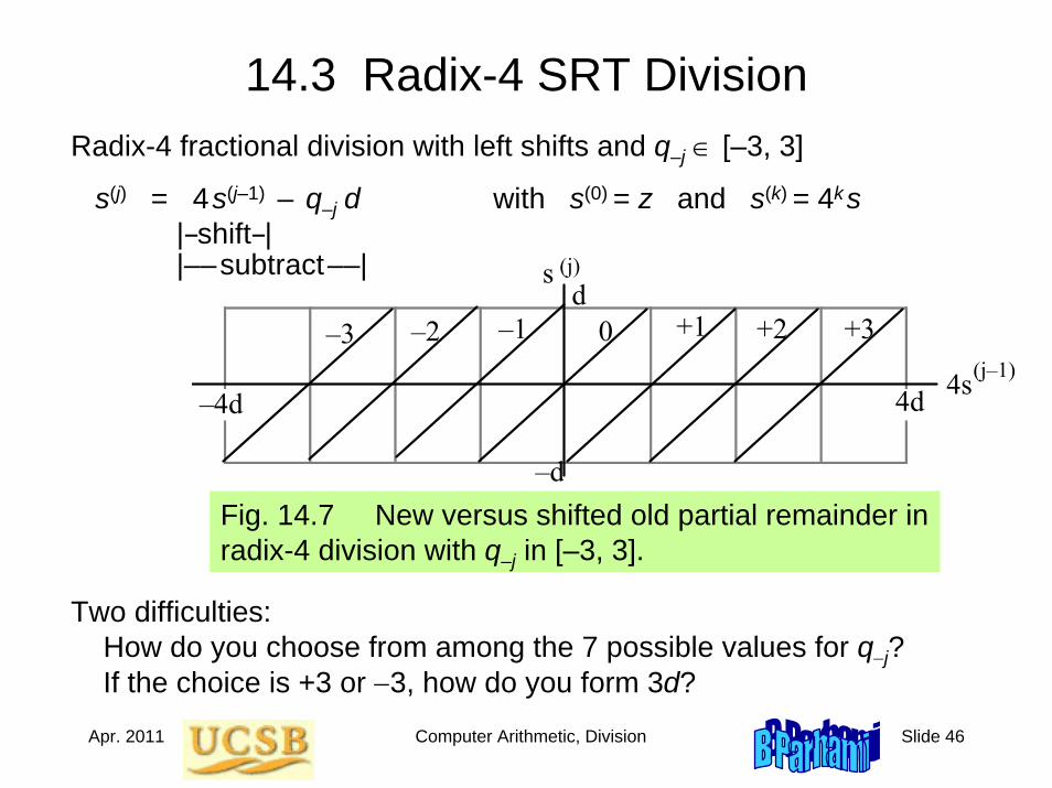
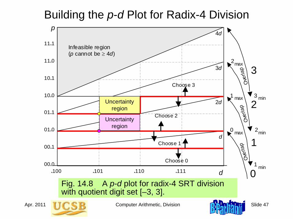
14.3 Radix-4 SRT Division
Fig. 14.7 New versus shifted old partial remainder in radix-4 division with q–j in [–3, 3].
–4d 4d
d
–d
4s(j–1)–3 –2 –1 0 +1 +2 +3
s (j)
Radix-4 fractional division with left shifts and q–j ∈ [–3, 3]
s(j) = 4s(j–1) – q–j d with s(0) = z and s(k) = 4ks|–shift–||––subtract––|
Two difficulties:How do you choose from among the 7 possible values for q−j?If the choice is +3 or −3, how do you form 3d?
Apr. 2011 Computer Arithmetic, Division Slide 47
Building the p-d Plot for Radix-4 Division
Fig. 14.8 A p-d plot for radix-4 SRT division with quotient digit set [–3, 3].
d
p
Infeasible region (p cannot be ≥ 4d)
.100 .101 .110 .111
10.1
10.0
01.1
00.0
00.1
01.0
11.1
11.0
d
2d
Choose 2
Choose 0
Choose 1
3
1
2 max
2 min
1 min
1 max
0 max
Ove
rlap
0
3d
4d
Choose 3
3 min
2
Ove
rlap
Ove
rlap
Uncertaintyregion
Uncertaintyregion
Apr. 2011 Computer Arithmetic, Division Slide 48
–4d 4d
d
–d
4s (j–1)
–3 –2 –1 0 +1 +2 +3
s (j)
2d/3
8d/3 –2d/3
–8d/3
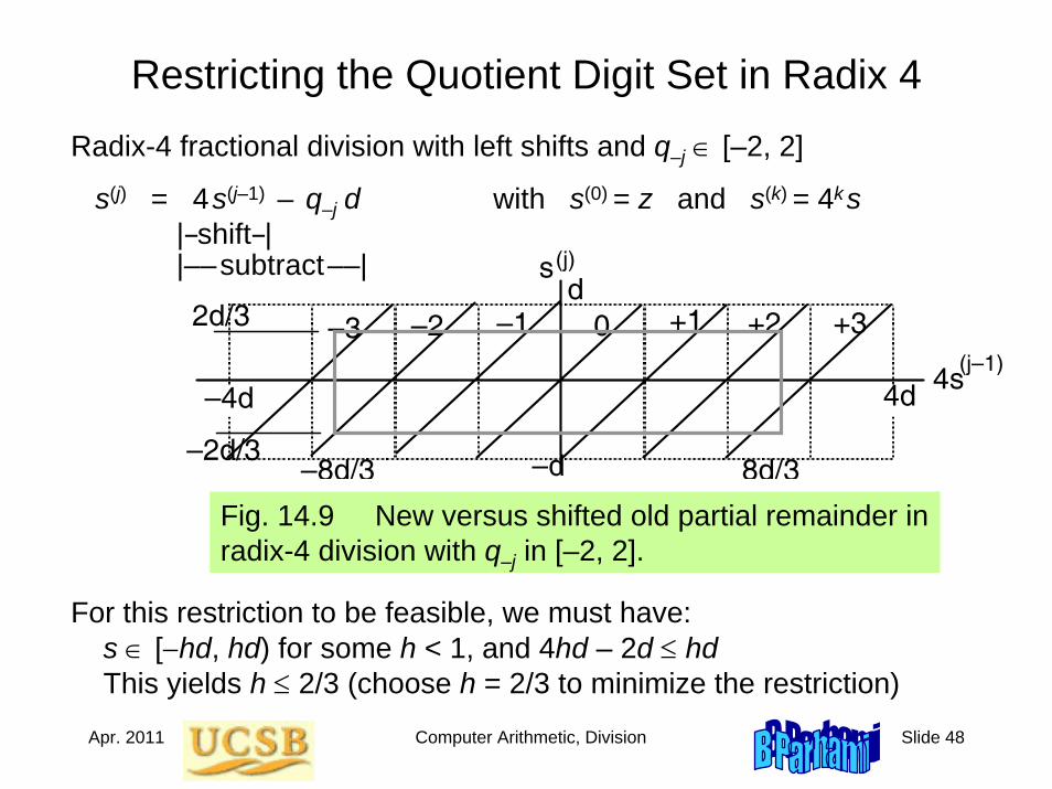
Restricting the Quotient Digit Set in Radix 4
Fig. 14.9 New versus shifted old partial remainder in radix-4 division with q–j in [–2, 2].
Radix-4 fractional division with left shifts and q–j ∈ [–2, 2]
s(j) = 4s(j–1) – q–j d with s(0) = z and s(k) = 4ks|–shift–||––subtract––|
For this restriction to be feasible, we must have:s ∈ [−hd, hd) for some h < 1, and 4hd – 2d ≤ hdThis yields h ≤ 2/3 (choose h = 2/3 to minimize the restriction)
Apr. 2011 Computer Arithmetic, Division Slide 49
d
p
.100 .101 .110 .111
10.1
10.0
01.1
00.0
00.1
01.0
11.1
11.0
Choose 2
Choose 0
Choose 1 1
2 min
1 min
2 max
1 max
0 max
0
2
Ove
rlap
Ove
rlap
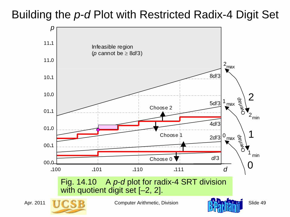
Infeasible region (p cannot be ≥ 8d/3)
8d/3
5d/3
4d/3
2d/3
d/3
Building the p-d Plot with Restricted Radix-4 Digit Set
Fig. 14.10 A p-d plot for radix-4 SRT division with quotient digit set [–2, 2].
Apr. 2011 Computer Arithmetic, Division Slide 50
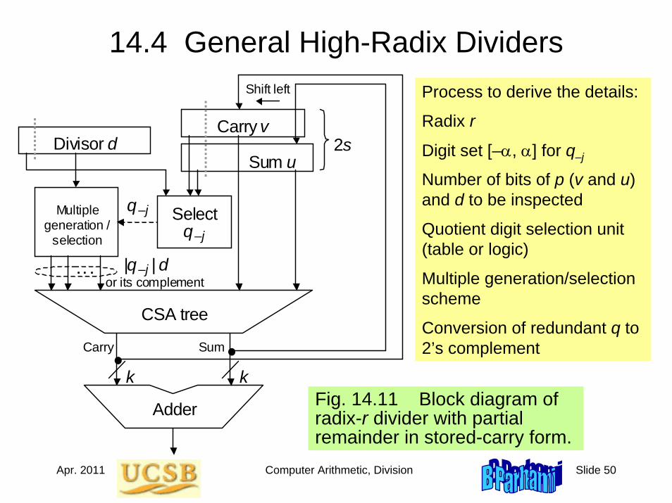
14.4 General High-Radix Dividers
Carry v
CSA tree
Adder
Divisor d
k k
Select q –j
Shift left
2s Sum u
Multiple generation /
selection
Carry Sum
q –j
. . . q –j | | d or its complement
Fig. 14.11 Block diagram of radix-r divider with partial remainder in stored-carry form.
Process to derive the details:
Radix r
Digit set [–α, α] for q–j
Number of bits of p (v and u) and d to be inspected
Quotient digit selection unit (table or logic)
Multiple generation/selection scheme
Conversion of redundant q to 2’s complement
Apr. 2011 Computer Arithmetic, Division Slide 51
14.5 Quotient Digit Selection
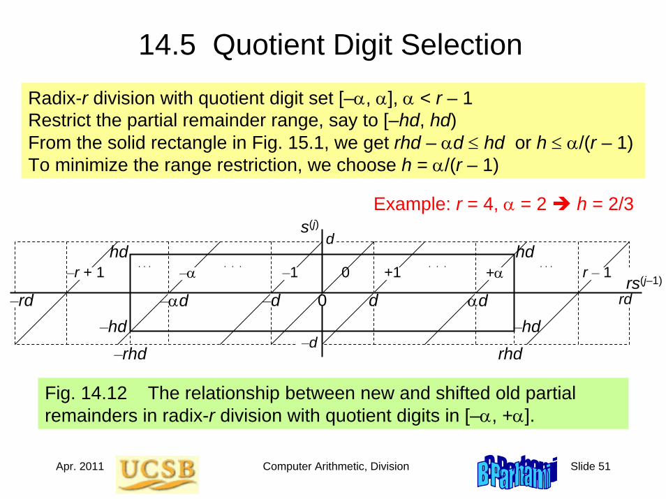
Radix-r division with quotient digit set [–α, α], α < r – 1 Restrict the partial remainder range, say to [–hd, hd)From the solid rectangle in Fig. 15.1, we get rhd – αd ≤ hd or h ≤ α/(r – 1) To minimize the range restriction, we choose h = α/(r – 1)
Fig. 14.12 The relationship between new and shifted old partial remainders in radix-r division with quotient digits in [–α, +α].
Example: r = 4, α = 2 h = 2/3
r – 1+10 +α–r + 1 –α –1
αdd
hd hd
–hd –hdrhd–rhd
–αd –d–rd rd
d
–d
. . . . . . . . . . . .
rs(j–1)
s(j)
0
Apr. 2011 Computer Arithmetic, Division Slide 52
Why Using Truncated p and d Values Is Acceptable
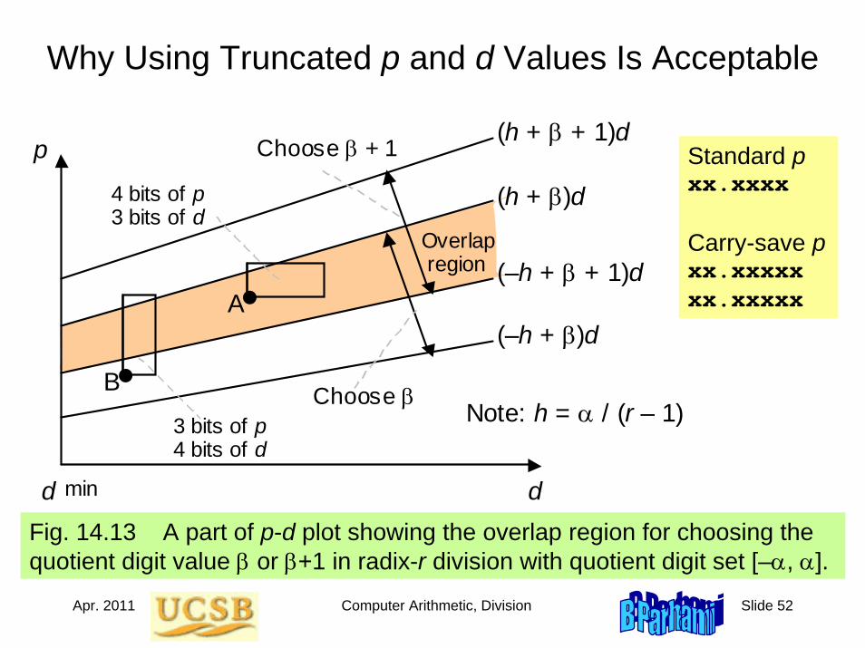
Fig. 14.13 A part of p-d plot showing the overlap region for choosing the quotient digit value β or β+1 in radix-r division with quotient digit set [–α, α].
p
d
Choose β + 1
Overlap region
A
Choose β
d min
(h + β + 1)d
(h + β)d
(–h + β + 1)d
(–h + β)d
B
4 bits of p 3 bits of d
3 bits of p 4 bits of d
Note: h = α / (r – 1)
Standard pxx.xxxx
Carry-save pxx.xxxxxxx.xxxxx

Apr. 2011 Computer Arithmetic, Division Slide 53
Table Entries in the Quotient Digit Selection Logic
Fig. 14.14 A part of p-d plot showing an overlap region and its staircase-like selection boundary.
p
d
β
+1(h + )d
(–h + )d
(h + + 1)d
(–h + + 1)d
Note: h = /(r–1)
β
β
β
β
β
αβ
β+1 ββ
ββ
ββ
ββ
β+1 β+1β+1 β+1
β+1 β+1β+1
β+1orδ+1δ
Origin
Apr. 2011 Computer Arithmetic, Division Slide 54
14.6 Using p-d Plots in Practice
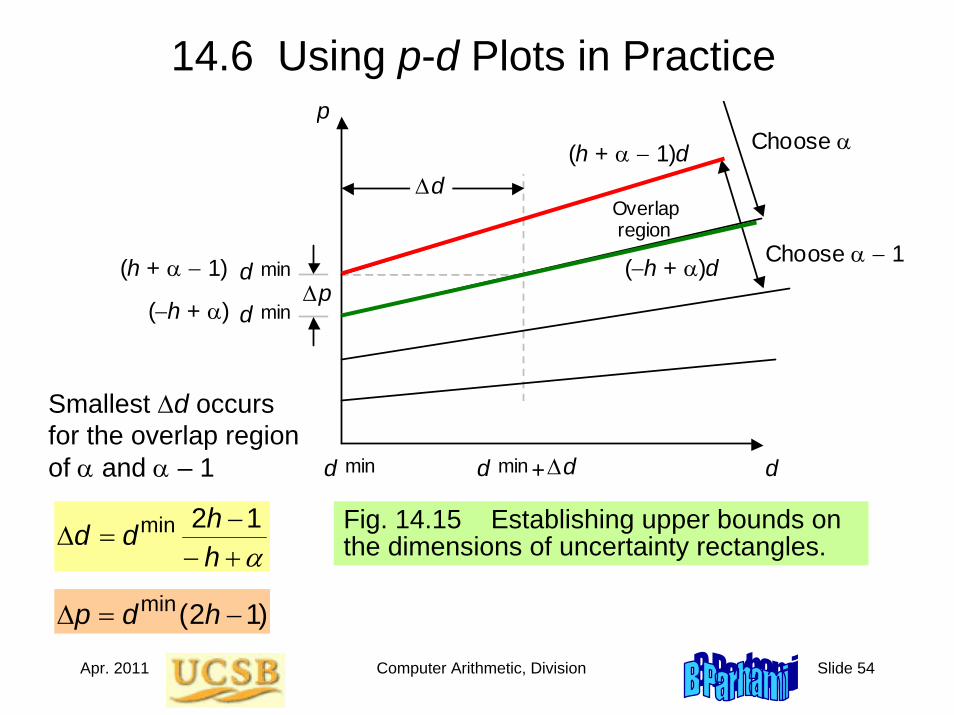
Fig. 14.15 Establishing upper bounds on the dimensions of uncertainty rectangles.
Δp
p
d
Choose α
Choose α − 1
d min
Overlap region
(h + α − 1)d
(−h + α)d
Δd
d min Δd +
(h + α − 1) d min
(−h + α) d min
Smallest Δd occurs for the overlap region of α and α – 1
α+−−
=Δhhdd 12min
)12(min −=Δ hdp
Apr. 2011 Computer Arithmetic, Division Slide 55
Example: Lower Bounds on Precision
)12(min −=Δ hdp
Fig. 14.15
Δp
p
d
Choose α
Choose α − 1
d min
Overlap region
(h + α − 1)d
(−h + α)d
Δd
d min Δd +
(h + α − 1) d min
(−h + α) d min
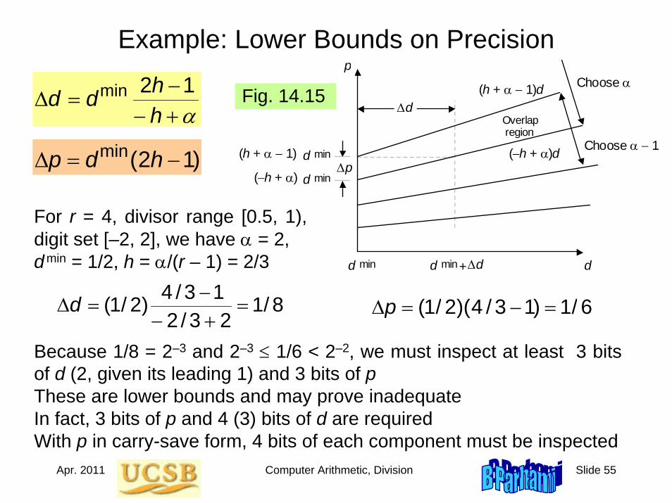
For r = 4, divisor range [0.5, 1), digit set [–2, 2], we have α = 2, dmin = 1/2, h = α/(r – 1) = 2/3
Because 1/8 = 2–3 and 2–3 ≤ 1/6 < 2–2, we must inspect at least 3 bits of d (2, given its leading 1) and 3 bits of p These are lower bounds and may prove inadequateIn fact, 3 bits of p and 4 (3) bits of d are required With p in carry-save form, 4 bits of each component must be inspected
8/123/2
13/4)2/1( =+−
−=Δd 6/1)13/4)(2/1( =−=Δp
α+−−
=Δhhdd 12min
Apr. 2011 Computer Arithmetic, Division Slide 56
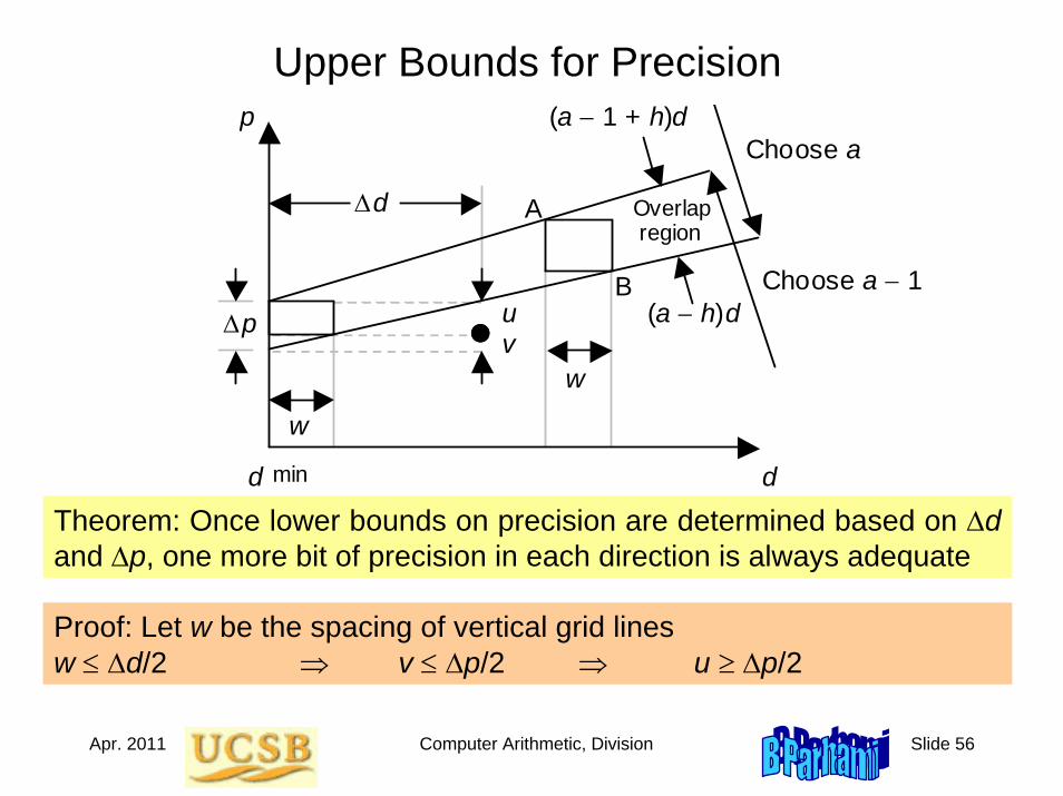
Upper Bounds for Precision
Theorem: Once lower bounds on precision are determined based on Δdand Δp, one more bit of precision in each direction is always adequate
u v
Δp
p
d
w
Choose a
Choose a − 1
d min
Overlap region
w
(a − 1 + h)d
(a − h)d
Δd A
B
Proof: Let w be the spacing of vertical grid linesw ≤ Δd/2 ⇒ v ≤ Δp/2 ⇒ u ≥ Δp/2
Apr. 2011 Computer Arithmetic, Division Slide 57
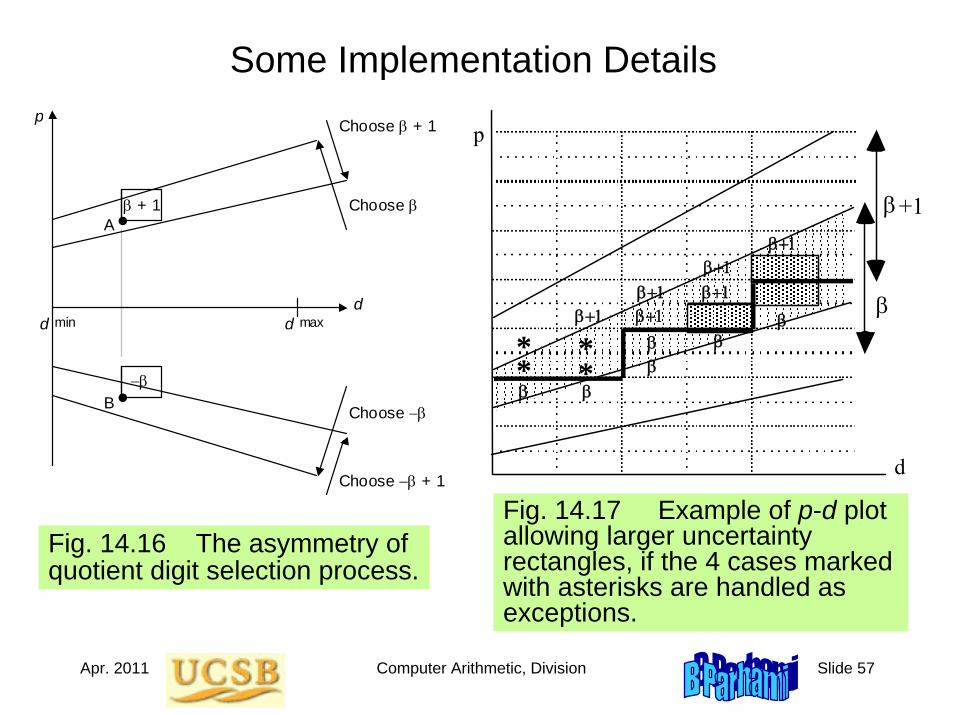
Some Implementation Details
Fig. 14.16 The asymmetry of quotient digit selection process.
p
d
Choose β + 1
Choose β
d min
A
B
d max
−β
β + 1
Choose −β + 1
Choose −β
p
d
β
+1
β
β
β
β β
β
δ β
β+1
β+1
β+1
β+1
β+1
β+1 or
δ+1
δ
*
* *
*
Fig. 14.17 Example of p-d plot allowing larger uncertainty rectangles, if the 4 cases marked with asterisks are handled as exceptions.
Apr. 2011 Computer Arithmetic, Division Slide 58
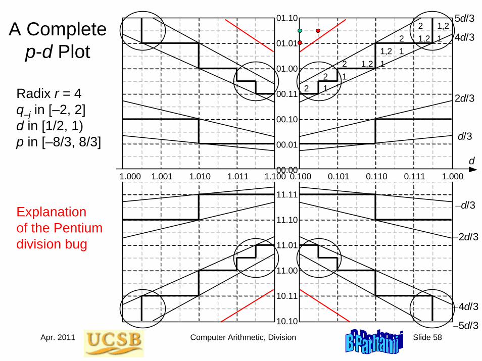
A Complete p-d Plot
5d/3
4d/3
d 1.000 1.001 1.010 1.011 1.100 0.100 0.101 0.110 0.111 1.000
01.10
01.01
01.00
00.11
00.10
00.00
00.01
11.11
11.10
11.01
11.00
10.11
10.10
2d/3
d/3
–d/3
–4d/3
–5d/3
–2d/3
2 1 2 1
2 1,2 1 1,2 1
2 1,2 1 2 1,2
Radix r = 4q–j in [–2, 2]d in [1/2, 1)p in [–8/3, 8/3]
Explanation of the Pentium division bug
Apr. 2011 Computer Arithmetic, Division Slide 59
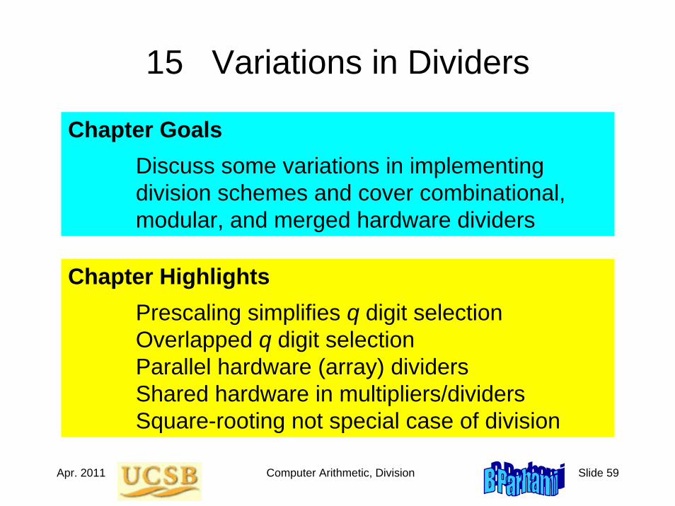
15 Variations in Dividers
Chapter GoalsDiscuss some variations in implementingdivision schemes and cover combinational,modular, and merged hardware dividers
Chapter HighlightsPrescaling simplifies q digit selectionOverlapped q digit selectionParallel hardware (array) dividersShared hardware in multipliers/dividersSquare-rooting not special case of division
Apr. 2011 Computer Arithmetic, Division Slide 60
Variations in Dividers: Topics
Topics in This Chapter
15.1 Division with Prescaling
15.2 Overlapped Quotient Digit Selection
15.3 Combinational and Array Dividers
15.4 Modular Dividers and Reducers
15.5 The Special Case of Reciprocation
15.6 Combined Multiply/Divide Units
Apr. 2011 Computer Arithmetic, Division Slide 61
15.1 Division with Prescaling
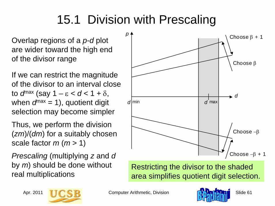
Restricting the divisor to the shaded area simplifies quotient digit selection.
p
d
Choose β + 1
Choose β
d min d max
Choose −β + 1
Choose −β
Overlap regions of a p-d plot are wider toward the high end of the divisor range
If we can restrict the magnitude of the divisor to an interval close to dmax (say 1 – ε < d < 1 + δ, when dmax = 1), quotient digit selection may become simpler
Thus, we perform the division (zm)/(dm) for a suitably chosen scale factor m (m > 1)
Prescaling (multiplying z and dby m) should be done without real multiplications
Apr. 2011 Computer Arithmetic, Division Slide 62
Examples of Prescaling
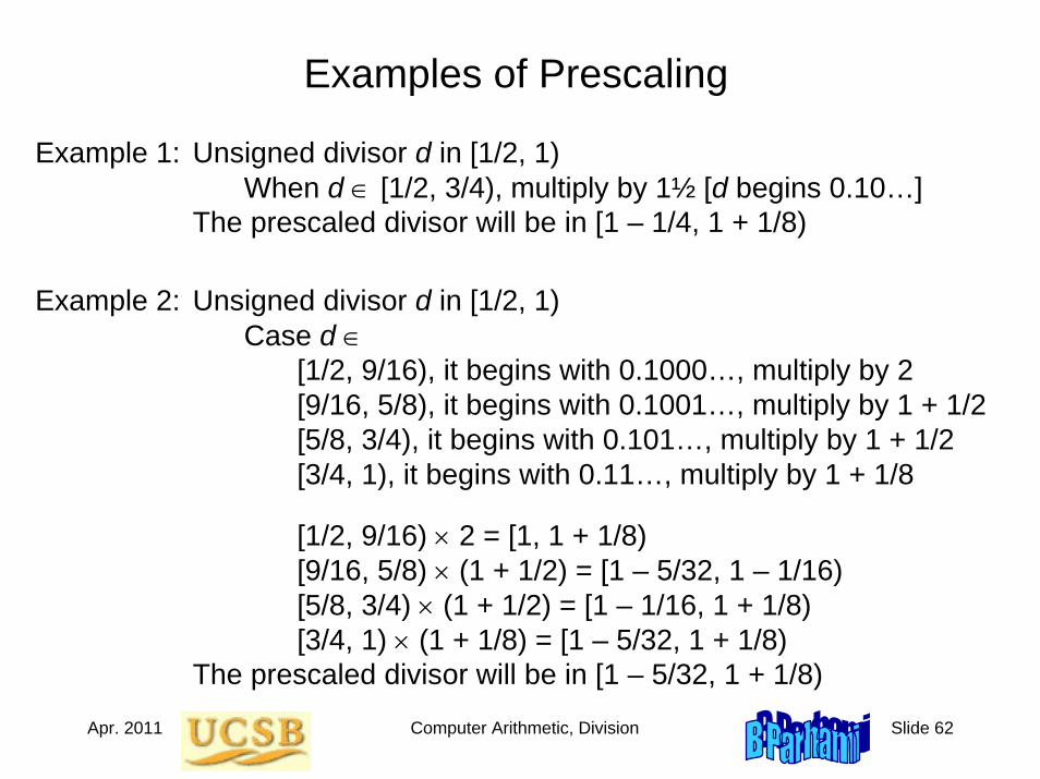
Example 1: Unsigned divisor d in [1/2, 1)When d ∈ [1/2, 3/4), multiply by 1½ [d begins 0.10…]
The prescaled divisor will be in [1 – 1/4, 1 + 1/8)
Example 2: Unsigned divisor d in [1/2, 1)Case d ∈
[1/2, 9/16), it begins with 0.1000…, multiply by 2 [9/16, 5/8), it begins with 0.1001…, multiply by 1 + 1/2 [5/8, 3/4), it begins with 0.101…, multiply by 1 + 1/2 [3/4, 1), it begins with 0.11…, multiply by 1 + 1/8
[1/2, 9/16) × 2 = [1, 1 + 1/8)[9/16, 5/8) × (1 + 1/2) = [1 – 5/32, 1 – 1/16)[5/8, 3/4) × (1 + 1/2) = [1 – 1/16, 1 + 1/8) [3/4, 1) × (1 + 1/8) = [1 – 5/32, 1 + 1/8)
The prescaled divisor will be in [1 – 5/32, 1 + 1/8)
Apr. 2011 Computer Arithmetic, Division Slide 63
15.2 Overlapped Quotient Digit Selection
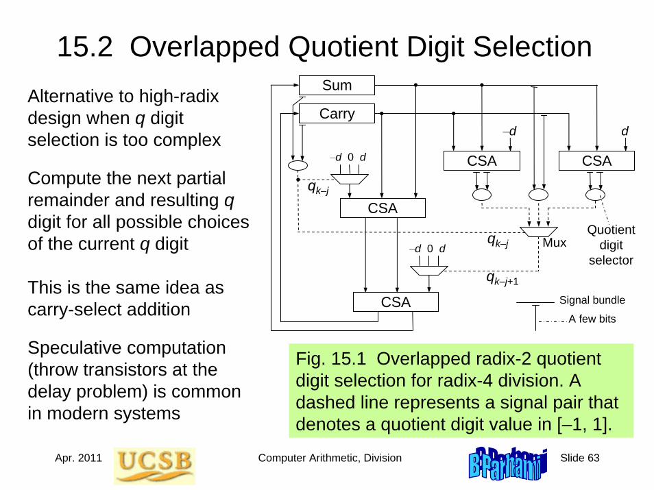
Fig. 15.1 Overlapped radix-2 quotient digit selection for radix-4 division. A dashed line represents a signal pair that denotes a quotient digit value in [–1, 1].
Alternative to high-radix design when q digit selection is too complex
Compute the next partial remainder and resulting q digit for all possible choices of the current q digit
–d 0 d
Sum
Carry
CSA
CSA CSA
–d d
–d 0 d
CSA
qk–j
qk–j+1
qk–j
Quotient digit
selectorMux
Signal bundle
A few bits
This is the same idea as carry-select addition
Speculative computation (throw transistors at the delay problem) is common in modern systems
Apr. 2011 Computer Arithmetic, Division Slide 64
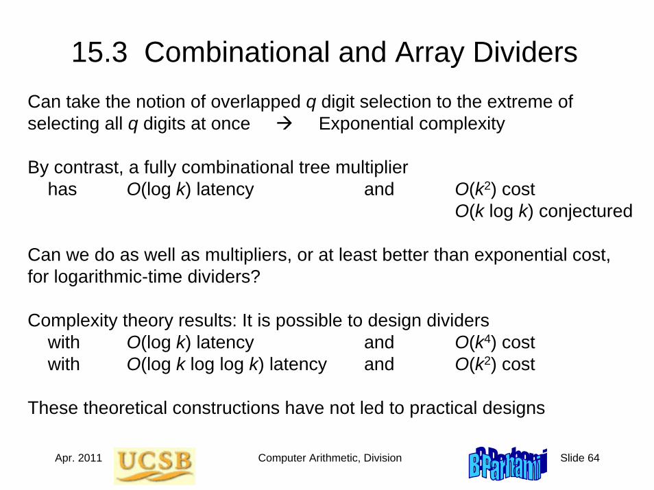
15.3 Combinational and Array DividersCan take the notion of overlapped q digit selection to the extreme of selecting all q digits at once Exponential complexity
By contrast, a fully combinational tree multiplier has O(log k) latency and O(k2) cost
O(k log k) conjectured
Can we do as well as multipliers, or at least better than exponential cost, for logarithmic-time dividers?
Complexity theory results: It is possible to design dividerswith O(log k) latency and O(k4) costwith O(log k log log k) latency and O(k2) cost
These theoretical constructions have not led to practical designs
Apr. 2011 Computer Arithmetic, Division Slide 65
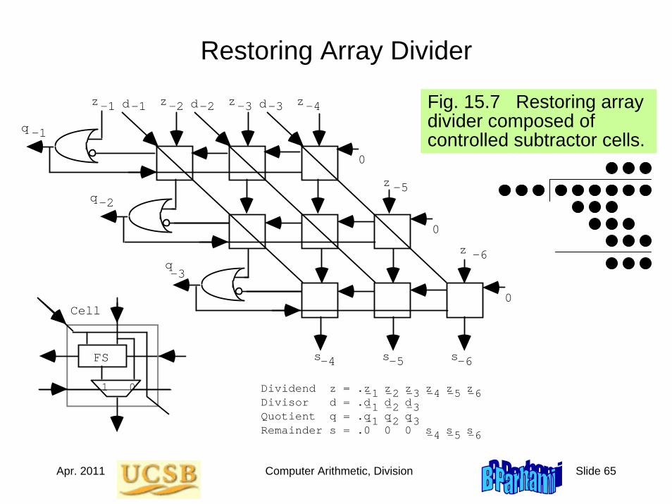
Restoring Array Divider
Fig. 15.7 Restoring array divider composed of controlled subtractor cells.
z
z
–5
–6
s s s –4 –5 –6
q
q
q
–1
–2
–3
FS
Cell
z z z z–1 –2 –3 –4
1 0
d d d –1 –2 –3
0
0
0
–1 –2 –3 –4 –5 –6 –1 –2 –3 –1 –2 –3 –4 –5 –6
Dividend z = .z z z z z z Divisor d = .d d d Quotient q = .q q q Remainder s = .0 0 0 s s s
Apr. 2011 Computer Arithmetic, Division Slide 66
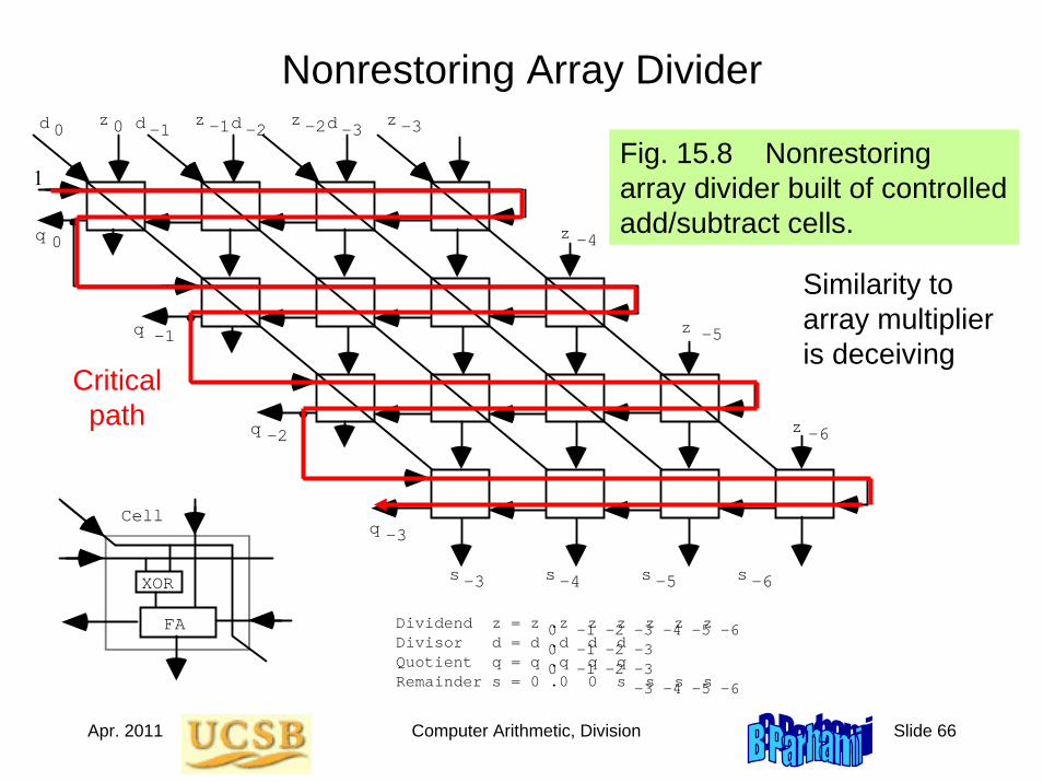
Nonrestoring Array Divider
Fig. 15.8 Nonrestoring array divider built of controlled add/subtract cells.
Dividend z = z .z z z z z z Divisor d = d .d d d Quotient q = q .q q q Remainder s = 0 .0 0 s s s s
0 –1 –2 –3 –4 –5 –6 0 –1 –2 –3 0 –1 –2 –3 –3 –4 –5 –6
z
z
z
–4
–5
–6
s s s s–3 –4 –5 –6
q
q
q
0
–1
–2
q –3
d d d d0 –1 –2 –3z z z z0 –1 –2 –3
FA
XOR
Cell
1
Similarity to array multiplier is deceiving
Critical path
Apr. 2011 Computer Arithmetic, Division Slide 67
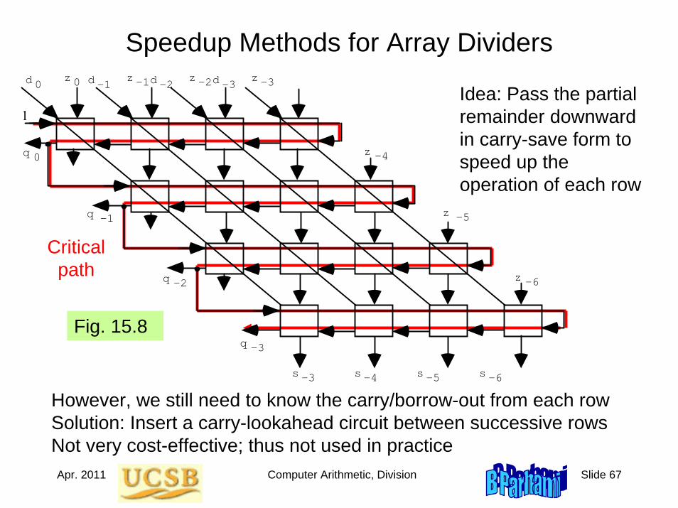
Speedup Methods for Array Dividers
Critical path
Dividend z = z .z z z z z z Divisor d = d .d d d Quotient q = q .q q q Remainder s = 0 .0 0 s s s s
0 –1 –2 –3 –4 –5 –6 0 –1 –2 –3 0 –1 –2 –3 –3 –4 –5 –6
z
z
z
–4
–5
–6
s s s s–3 –4 –5 –6
q
q
q
0
–1
–2
q –3
d d d d0 –1 –2 –3z z z z0 –1 –2 –3
FA
XOR
Cell
1
However, we still need to know the carry/borrow-out from each rowSolution: Insert a carry-lookahead circuit between successive rowsNot very cost-effective; thus not used in practice
Idea: Pass the partial remainder downward in carry-save form to speed up the operation of each row
Fig. 15.8
Apr. 2011 Computer Arithmetic, Division Slide 68
15.4 Modular Dividers and Reducers
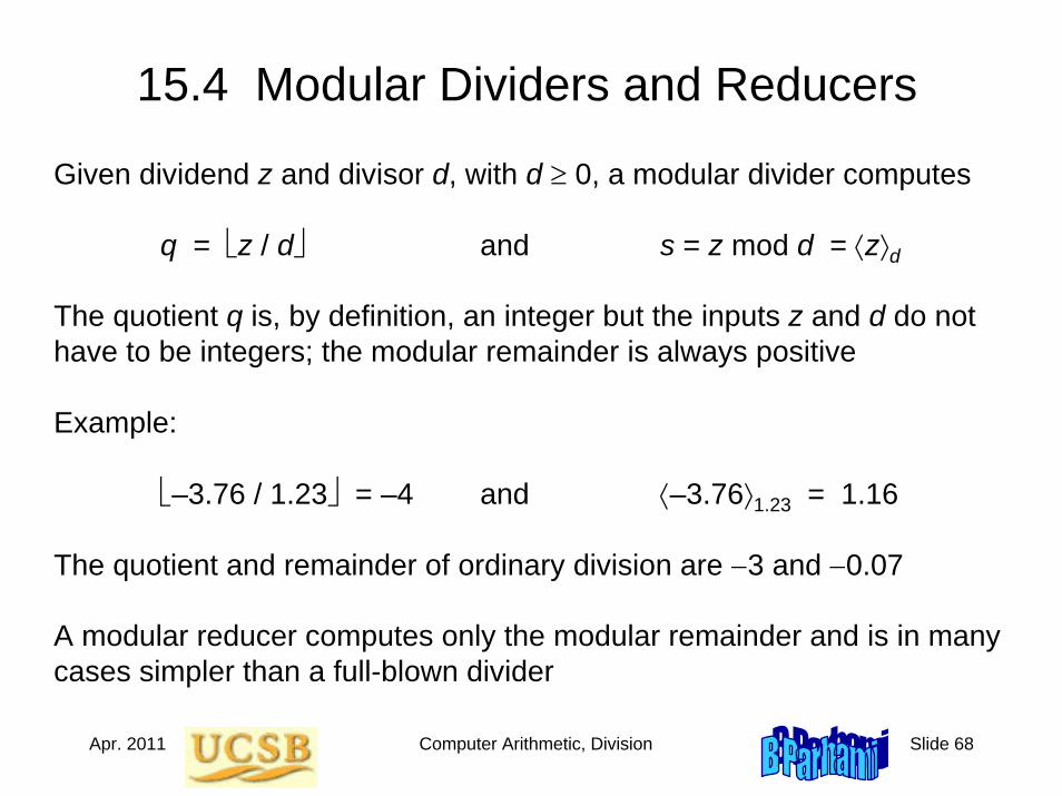
Given dividend z and divisor d, with d ≥ 0, a modular divider computes
q = ⎣z / d⎦ and s = z mod d = ⟨z⟩d
The quotient q is, by definition, an integer but the inputs z and d do not have to be integers; the modular remainder is always positive
Example:
⎣–3.76 / 1.23⎦ = –4 and ⟨–3.76⟩1.23 = 1.16
The quotient and remainder of ordinary division are −3 and −0.07
A modular reducer computes only the modular remainder and is in many cases simpler than a full-blown divider
Apr. 2011 Computer Arithmetic, Division Slide 69
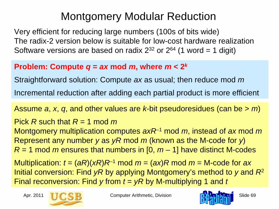
Montgomery Modular ReductionVery efficient for reducing large numbers (100s of bits wide)The radix-2 version below is suitable for low-cost hardware realizationSoftware versions are based on radix 232 or 264 (1 word = 1 digit)
Assume a, x, q, and other values are k-bit pseudoresidues (can be > m)
Pick R such that R = 1 mod mMontgomery multiplication computes axR–1 mod m, instead of ax mod mRepresent any number y as yR mod m (known as the M-code for y)R = 1 mod m ensures that numbers in [0, m – 1] have distinct M-codes
Multiplication: t = (aR)(xR)R–1 mod m = (ax)R mod m = M-code for axInitial conversion: Find yR by applying Montgomery’s method to y and R2
Final reconversion: Find y from t = yR by M-multiplying 1 and t
Problem: Compute q = ax mod m, where m < 2k
Straightforward solution: Compute ax as usual; then reduce mod m
Incremental reduction after adding each partial product is more efficient
Apr. 2011 Computer Arithmetic, Division Slide 70
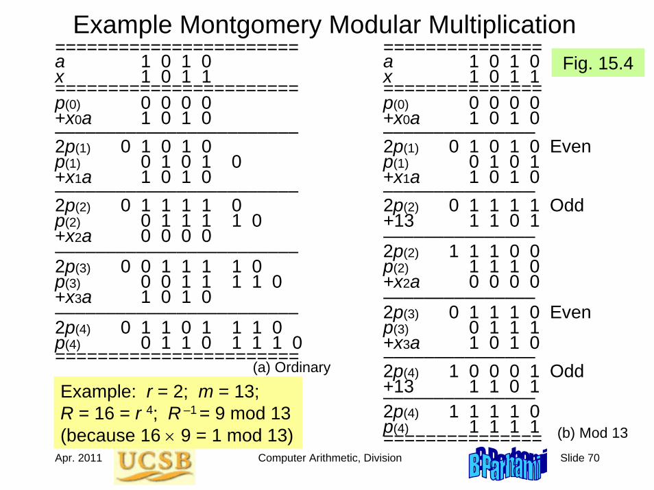
Example Montgomery Modular Multiplication======================= ===============a 1 0 1 0 a 1 0 1 0x 1 0 1 1 x 1 0 1 1======================= ===============p(0) 0 0 0 0 p(0) 0 0 0 0+x0a 1 0 1 0 +x0a 1 0 1 0–––––––––––––––––––––––– –––––––––––––––2p(1) 0 1 0 1 0 2p(1) 0 1 0 1 0 Evenp(1) 0 1 0 1 0 p(1) 0 1 0 1 +x1a 1 0 1 0 +x1a 1 0 1 0–––––––––––––––––––––––– –––––––––––––––2p(2) 0 1 1 1 1 0 2p(2) 0 1 1 1 1 Oddp(2) 0 1 1 1 1 0 +13 1 1 0 1+x2a 0 0 0 0 ––––––––––––––––––––––––––––––––––––––– 2p(2) 1 1 1 0 02p(3) 0 0 1 1 1 1 0 p(2) 1 1 1 0p(3) 0 0 1 1 1 1 0 +x2a 0 0 0 0+x3a 1 0 1 0 ––––––––––––––––––––––––––––––––––––––– 2p(3) 0 1 1 1 0 Even2p(4) 0 1 1 0 1 1 1 0 p(3) 0 1 1 1p(4) 0 1 1 0 1 1 1 0 +x3a 1 0 1 0======================= –––––––––––––––
2p(4) 1 0 0 0 1 Odd+13 1 1 0 1–––––––––––––––2p(4) 1 1 1 1 0p(4) 1 1 1 1===============
Example: r = 2; m = 13; R = 16 = r 4; R –1 = 9 mod 13 (because 16 × 9 = 1 mod 13)
Fig. 15.4
(a) Ordinary
(b) Mod 13
Apr. 2011 Computer Arithmetic, Division Slide 71
Advantages of Montgomery’s Method
Standard reduction is based on subtracting a multiple of m from the result depending on the most significant bit(s)
However, MSBs are not readily known if we use carry-save numbers
In Montgomery reduction, the decision is based on LSB(s), thus allowing the use of carry-save arithmetic as well as parallel processing
Apr. 2011 Computer Arithmetic, Division Slide 72
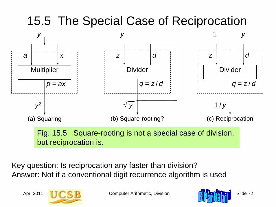
15.5 The Special Case of Reciprocation
(a) Squaring (b) Square-rooting?
Multiplier
p = ax
a x
y
y2
Divider
q = z / d
z d
y
√ y
(c) Reciprocation
Divider
q = z / d
z d
1 / y
y1
Fig. 15.5 Square-rooting is not a special case of division, but reciprocation is.
Key question: Is reciprocation any faster than division?Answer: Not if a conventional digit recurrence algorithm is used
Apr. 2011 Computer Arithmetic, Division Slide 73
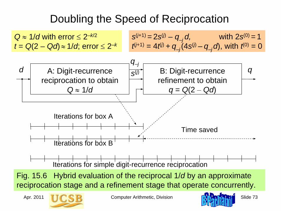
Doubling the Speed of ReciprocationQ ≈ 1/d with error ≤ 2–k/2
t = Q(2 – Qd) ≈ 1/d; error ≤ 2–k
Fig. 15.6 Hybrid evaluation of the reciprocal 1/d by an approximate reciprocation stage and a refinement stage that operate concurrently.
A: Digit-recurrence reciprocation to obtain
Q ≈ 1/d
Time saved
d B: Digit-recurrence refinement to obtain
q = Q(2 – Qd)
qq–j
Iterations for box A
Iterations for box B
Iterations for simple digit-recurrence reciprocation
s(j)
s(j+1) = 2s(j) – q–j d, with 2s(0) = 1t(j+1) = 4t(j) + q–j (4s(j) – q–j d), with t(0) = 0
Apr. 2011 Computer Arithmetic, Division Slide 74
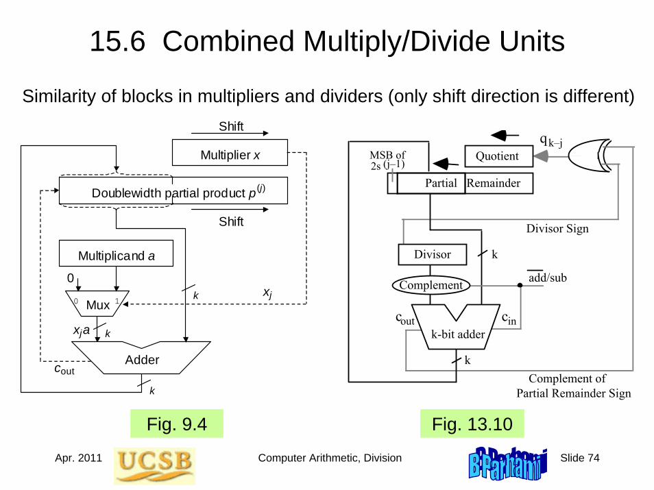
15.6 Combined Multiply/Divide Units
Quotient
k
Partial Remainder
Divisor
add/sub
k-bit adder
k
cout cin
Complement
qk–j 2s (j–1)MSB of
Divisor Sign
Complement of Partial Remainder Sign
Fig. 9.4 Fig. 13.10
Multiplier x
Mux
Adder
0
out c
0 1
Doublewidth partial product p
Multiplicand a
Shift
Shift
(j)
j x
x a j
k
k
k
Similarity of blocks in multipliers and dividers (only shift direction is different)
Apr. 2011 Computer Arithmetic, Division Slide 75
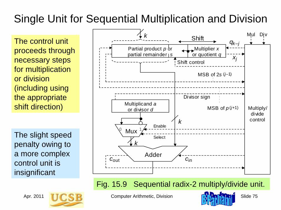
Single Unit for Sequential Multiplication and Division
The control unit proceeds through necessary steps for multiplication or division (including using the appropriate shift direction)
Fig. 15.9 Sequential radix-2 multiply/divide unit.
Multiplier x or quotient q
Mux
Adder out c
0 1
Partial product p or partial remainder s
Multiplicand a or divisor d
Shift control
Shift
Enable
in c
q k–j
MSB of 2s (j–1)
k
k
k
j x
MSB of p (j+1)
Divisor sign
Multiply/ divide control
Select
Mul Div
The slight speed penalty owing to a more complex control unit is insignificant
Apr. 2011 Computer Arithmetic, Division Slide 76
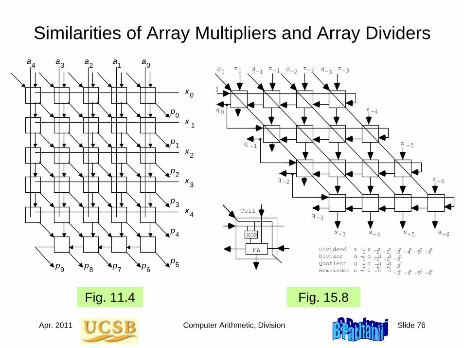
Similarities of Array Multipliers and Array Dividers
Dividend z = z .z z z z z z Divisor d = d .d d d Quotient q = q .q q q Remainder s = 0 .0 0 s s s s
0 –1 –2 –3 –4 –5 –6 0 –1 –2 –3 0 –1 –2 –3 –3 –4 –5 –6
z
z
z
–4
–5
–6
s s s s–3 –4 –5 –6
q
q
q
0
–1
–2
q–3
d d d d0 –1 –2 –3z z z z0 –1 –2 –3
FA
XOR
Cell
1
Fig. 11.4 Fig. 15.8
p p p p p
4 3 2 1 0 a a a a a
4
3
2
1
0
x
x
x
x
x
4
3
2
1
0
p
p
p
p
p
9 8 7 6 5
Apr. 2011 Computer Arithmetic, Division Slide 77
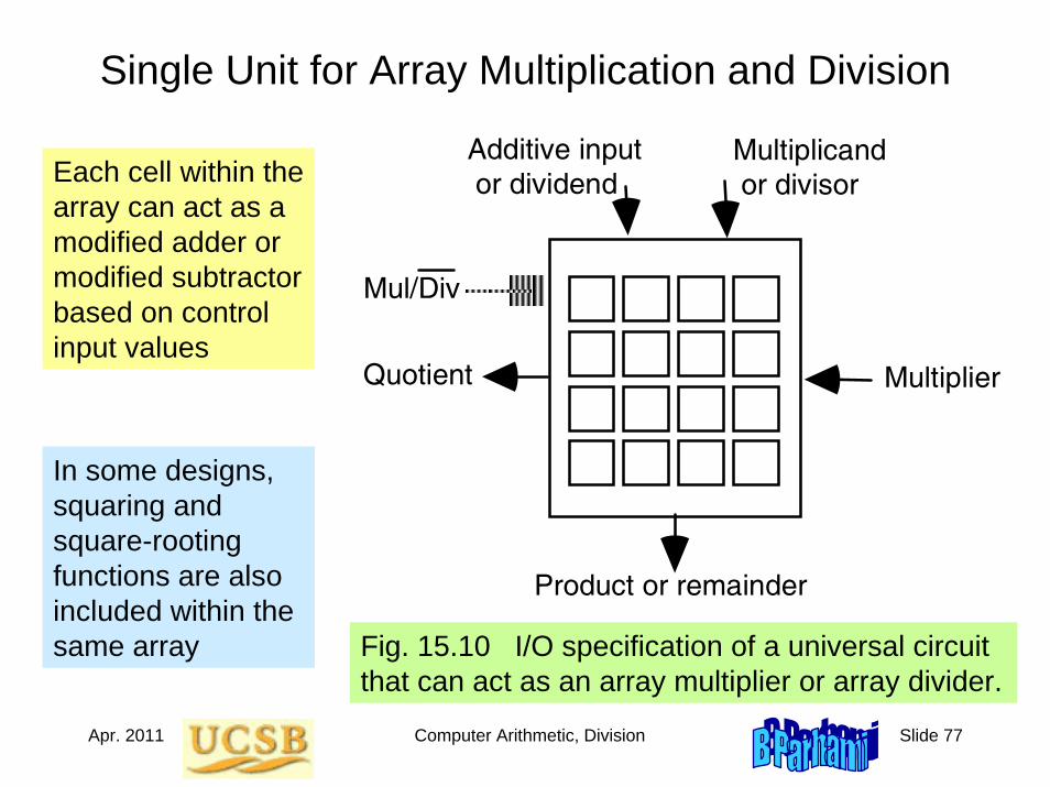
Single Unit for Array Multiplication and Division
Each cell within the array can act as a modified adder or modified subtractor based on control input values
Fig. 15.10 I/O specification of a universal circuit that can act as an array multiplier or array divider.
In some designs, squaring and square-rooting functions are also included within the same array
Multiplicand or divisor
Multiplier
Product or remainder
Quotient
Mul/Div
Additive input or dividend
Apr. 2011 Computer Arithmetic, Division Slide 78
16 Division by Convergence
Chapter GoalsShow how by using multiplication as thebasic operation in each division step,the number of iterations can be reduced
Chapter HighlightsDigit-recurrence as convergence methodConvergence by Newton-Raphson iterationComputing the reciprocal of a numberHardware implementation and fine tuning
Apr. 2011 Computer Arithmetic, Division Slide 79
Division by Convergence: Topics
Topics in This Chapter
16.1 General Convergence Methods
16.2 Division by Repeated Multiplications
16.3 Division by Reciprocation
16.4 Speedup of Convergence Division
16.5 Hardware Implementation
16.6 Analysis of Lookup Table Size
Apr. 2011 Computer Arithmetic, Division Slide 80
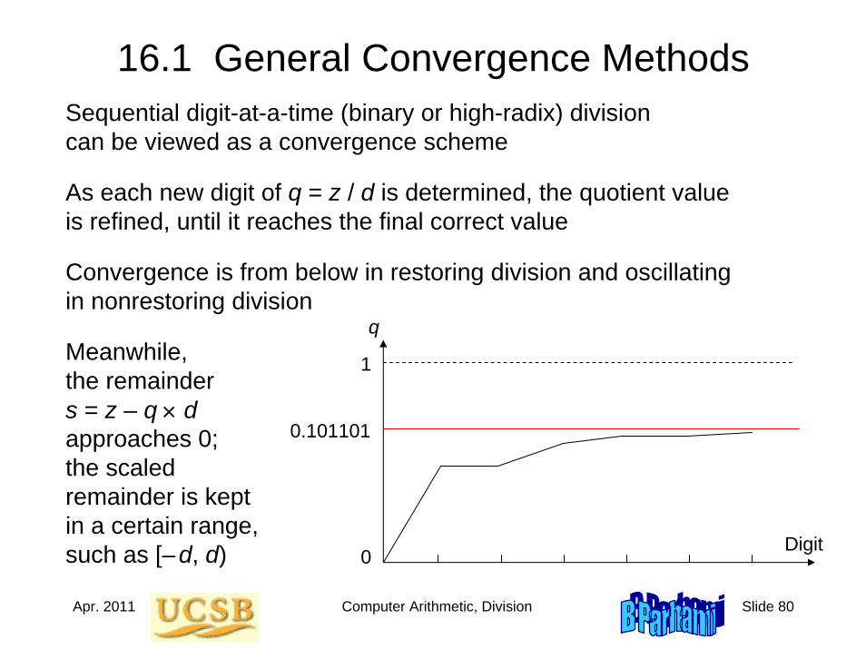
16.1 General Convergence MethodsSequential digit-at-a-time (binary or high-radix) division can be viewed as a convergence scheme
As each new digit of q = z / d is determined, the quotient value is refined, until it reaches the final correct value
Digit
0.101101
q
0
1
Convergence is from below in restoring division and oscillating in nonrestoring division
Meanwhile, the remainders = z – q × dapproaches 0; the scaled remainder is kept in a certain range, such as [–d, d)
Apr. 2011 Computer Arithmetic, Division Slide 81
Recurrence Formulas for Convergence Methods
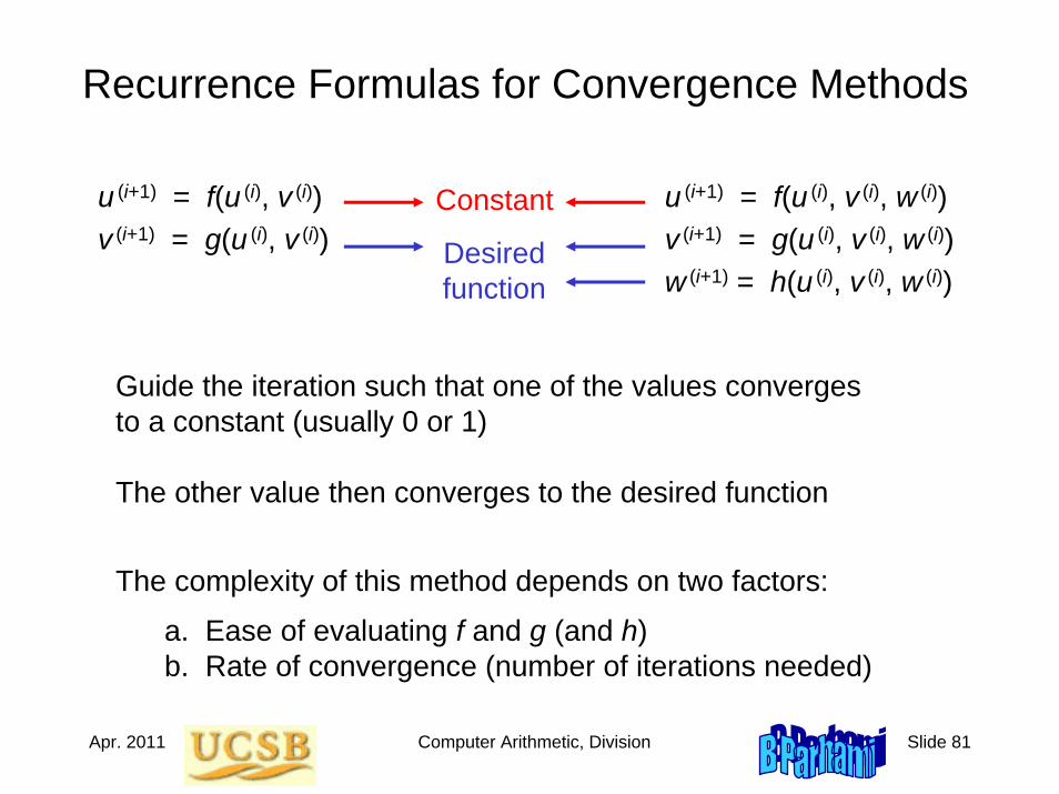
u (i+1) = f(u (i), v (i), w (i))v (i+1) = g(u (i), v (i), w (i))w (i+1) = h(u (i), v (i), w (i))
u (i+1) = f(u (i), v (i))v (i+1) = g(u (i), v (i))
The complexity of this method depends on two factors:
a. Ease of evaluating f and g (and h)b. Rate of convergence (number of iterations needed)
Constant
Desiredfunction
Guide the iteration such that one of the values converges to a constant (usually 0 or 1)
The other value then converges to the desired function
Apr. 2011 Computer Arithmetic, Division Slide 82
16.2 Division by Repeated Multiplications
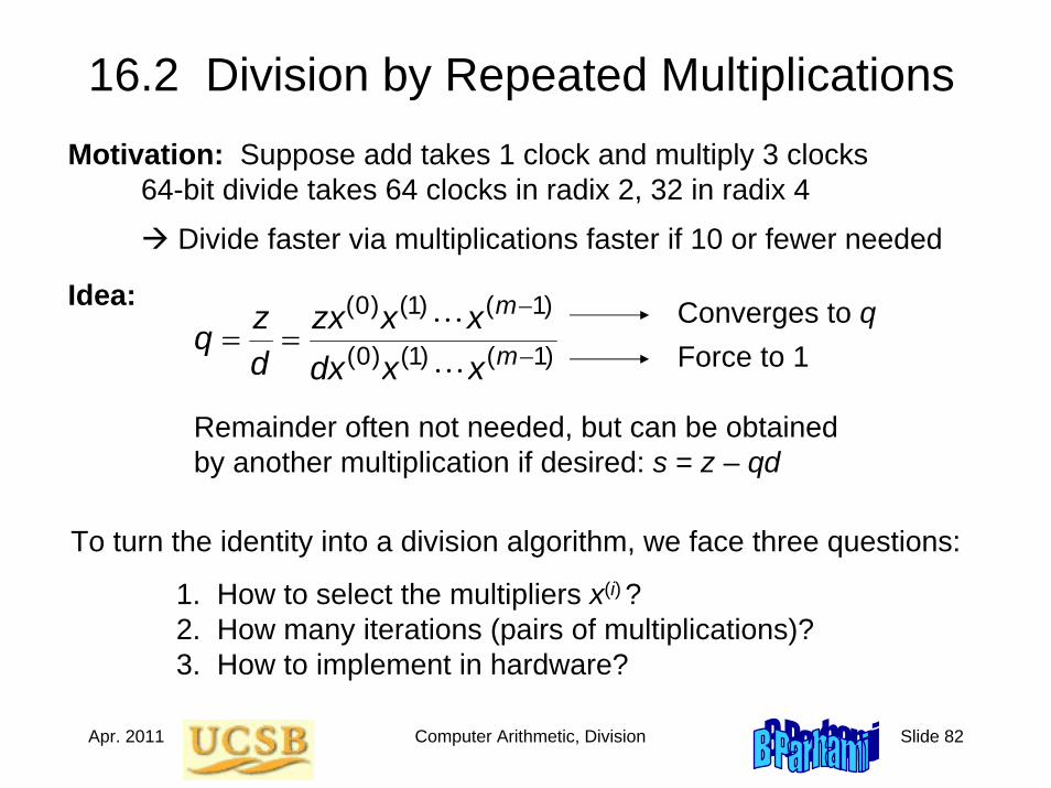
Remainder often not needed, but can be obtained by another multiplication if desired: s = z – qd
Motivation: Suppose add takes 1 clock and multiply 3 clocks64-bit divide takes 64 clocks in radix 2, 32 in radix 4
Divide faster via multiplications faster if 10 or fewer needed
)1()1()0(
)1()1()0(
−
−== m
m
xxdxxxzx
dzq
L
LIdea:
Force to 1Converges to q
To turn the identity into a division algorithm, we face three questions:
1. How to select the multipliers x(i) ?2. How many iterations (pairs of multiplications)? 3. How to implement in hardware?
Apr. 2011 Computer Arithmetic, Division Slide 83
Formulation as a Convergence Computation
)1()1()0(
)1()1()0(
−
−== m
m
xxdxxxzx
dzq
L
LIdea:
Force to 1Converges to q
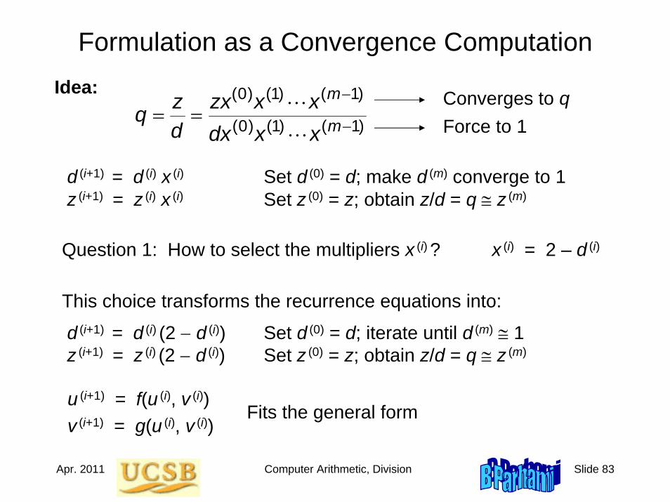
d (i+1) = d (i) x (i) Set d (0) = d; make d (m) converge to 1z (i+1) = z (i) x (i) Set z (0) = z; obtain z/d = q ≅ z (m)
Question 1: How to select the multipliers x (i) ? x (i) = 2 – d (i)
This choice transforms the recurrence equations into:
d (i+1) = d (i) (2 − d (i)) Set d (0) = d; iterate until d (m) ≅ 1z (i+1) = z (i) (2 − d (i)) Set z (0) = z; obtain z/d = q ≅ z (m)
u (i+1) = f(u (i), v (i))v (i+1) = g(u (i), v (i))
Fits the general form
Apr. 2011 Computer Arithmetic, Division Slide 84
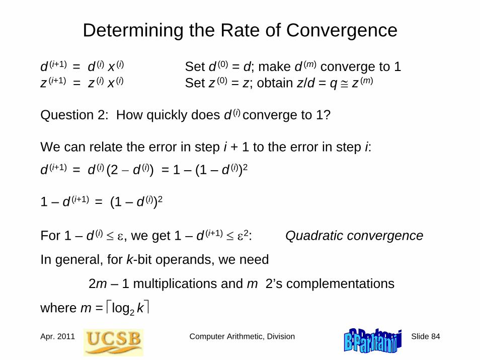
Determining the Rate of Convergence
d (i+1) = d (i) x (i) Set d (0) = d; make d (m) converge to 1z (i+1) = z (i) x (i) Set z (0) = z; obtain z/d = q ≅ z (m)
Question 2: How quickly does d (i) converge to 1?
We can relate the error in step i + 1 to the error in step i:
d (i+1) = d (i) (2 − d (i)) = 1 – (1 – d (i))2
1 – d (i+1) = (1 – d (i))2
For 1 – d (i) ≤ ε, we get 1 – d (i+1) ≤ ε2: Quadratic convergence
In general, for k-bit operands, we need
2m – 1 multiplications and m 2’s complementations
where m = ⎡log2 k⎤
Apr. 2011 Computer Arithmetic, Division Slide 85
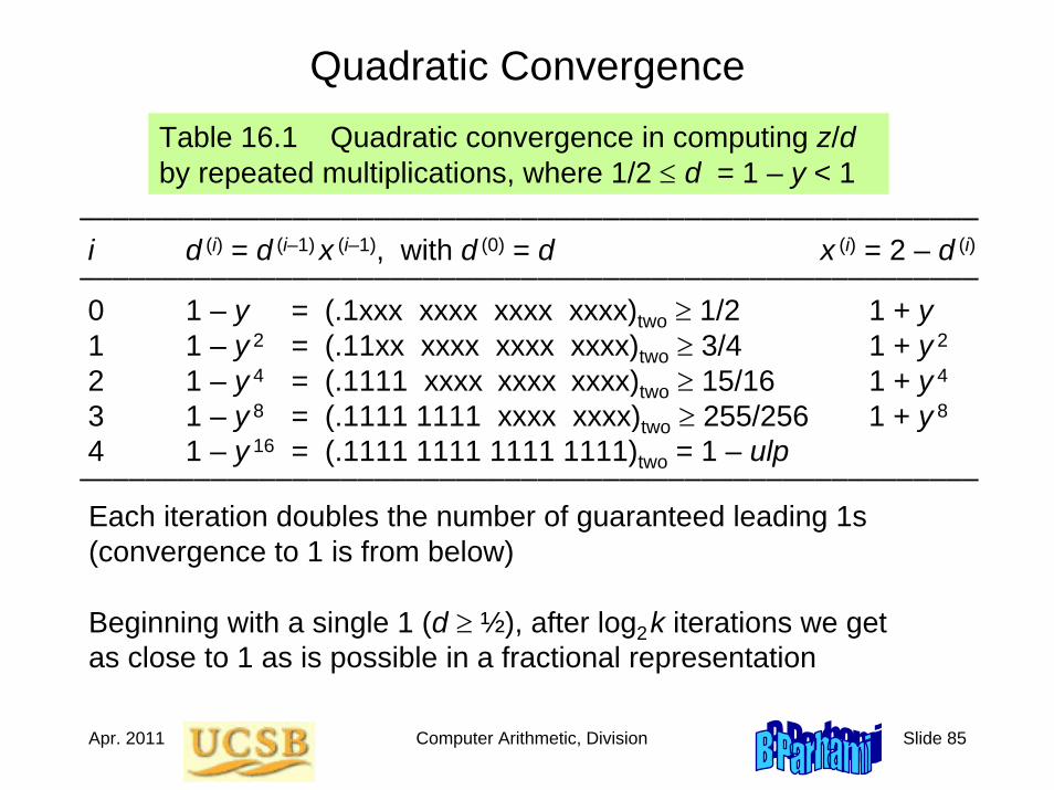
Quadratic ConvergenceTable 16.1 Quadratic convergence in computing z/dby repeated multiplications, where 1/2 ≤ d = 1 – y < 1
–––––––––––––––––––––––––––––––––––––––––––––––––––––––i d (i) = d (i–1) x (i–1), with d (0) = d x (i) = 2 – d (i)
–––––––––––––––––––––––––––––––––––––––––––––––––––––––0 1 – y = (.1xxx xxxx xxxx xxxx)two ≥ 1/2 1 + y1 1 – y 2 = (.11xx xxxx xxxx xxxx)two ≥ 3/4 1 + y 2
2 1 – y 4 = (.1111 xxxx xxxx xxxx)two ≥ 15/16 1 + y 4
3 1 – y 8 = (.1111 1111 xxxx xxxx)two ≥ 255/256 1 + y 8
4 1 – y 16 = (.1111 1111 1111 1111)two = 1 – ulp–––––––––––––––––––––––––––––––––––––––––––––––––––––––Each iteration doubles the number of guaranteed leading 1s (convergence to 1 is from below)
Beginning with a single 1 (d ≥ ½), after log2k iterations we get as close to 1 as is possible in a fractional representation
Apr. 2011 Computer Arithmetic, Division Slide 86
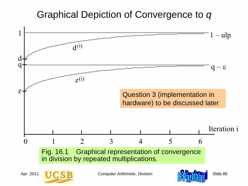
Graphical Depiction of Convergence to q
Fig. 16.1 Graphical representation of convergence in division by repeated multiplications.
1 1 – ulp
d
z
q –
Iteration i
d
z
0 1 2 3 4 5 6
(i)
(i)
q ε
Question 3 (implementation in hardware) to be discussed later
Apr. 2011 Computer Arithmetic, Division Slide 87
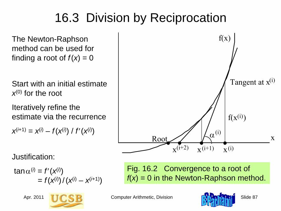
16.3 Division by Reciprocation
Fig. 16.2 Convergence to a root of f(x) = 0 in the Newton-Raphson method.
The Newton-Raphson method can be used for finding a root of f (x) = 0
f(x)
xx(i+1)x
f(x )
Tangent at x(i)
Root α x(i)(i+2)
(i)
(i)
Start with an initial estimate x(0) for the root
Iteratively refine the estimate via the recurrence
x(i+1) = x(i) – f (x(i)) / f ′(x(i))
Justification:
tan α(i) = f ′(x(i))= f (x(i)) / (x(i) – x(i+1))
Apr. 2011 Computer Arithmetic, Division Slide 88
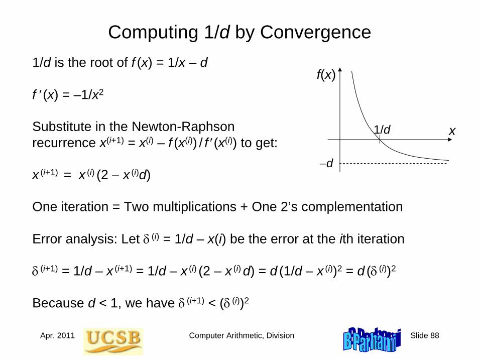
Computing 1/d by Convergence1/d is the root of f (x) = 1/x – d
f ′(x) = –1/x2
Substitute in the Newton-Raphson recurrence x(i+1) = x(i) – f (x(i)) / f ′(x(i)) to get:
x (i+1) = x (i) (2 − x (i)d)
One iteration = Two multiplications + One 2’s complementation
Error analysis: Let δ (i) = 1/d – x(i) be the error at the ith iteration
δ (i+1) = 1/d – x (i+1) = 1/d – x (i) (2 – x (i) d) = d (1/d – x (i))2 = d (δ (i))2
Because d < 1, we have δ (i+1) < (δ (i))2
−d
1/d x
f(x)
Apr. 2011 Computer Arithmetic, Division Slide 89
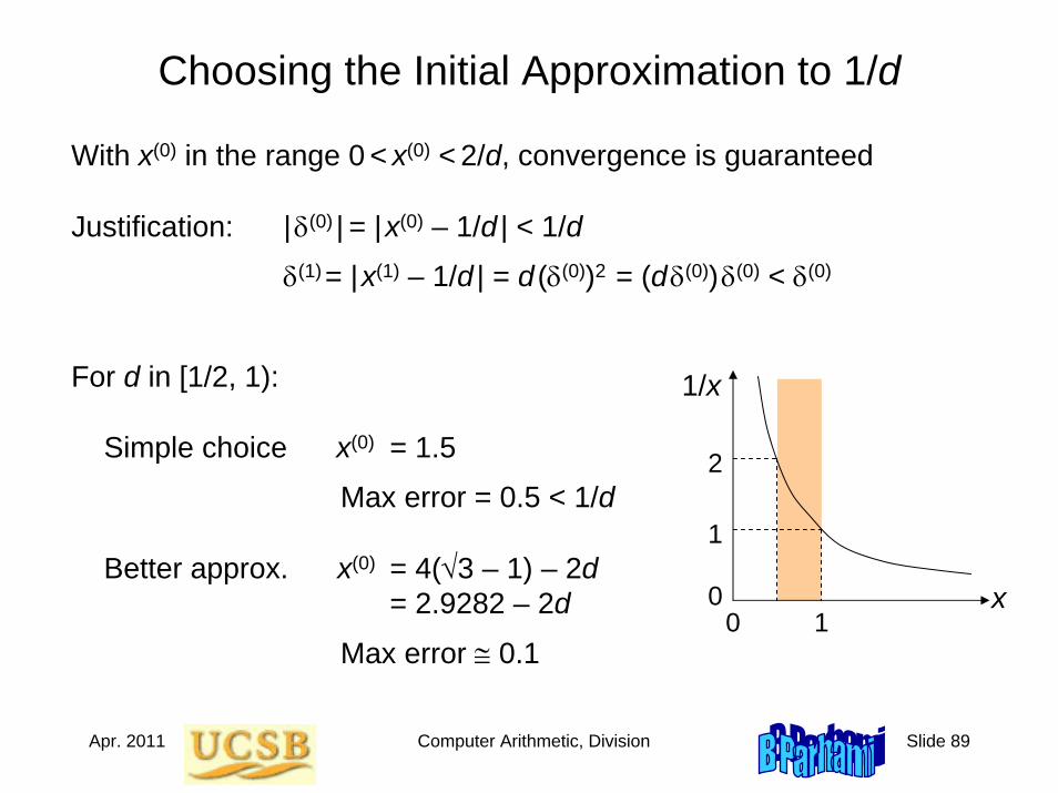
Choosing the Initial Approximation to 1/d
With x(0) in the range 0 < x(0) < 2/d, convergence is guaranteed
Justification: |δ(0) | = |x(0) – 1/d | < 1/d
δ(1)= |x(1) – 1/d | = d (δ(0))2 = (dδ(0))δ(0) < δ(0)
1
x
1/x
2
10
0
For d in [1/2, 1):
Simple choice x(0) = 1.5
Max error = 0.5 < 1/d
Better approx. x(0) = 4(√3 – 1) – 2d= 2.9282 – 2d
Max error ≅ 0.1
Apr. 2011 Computer Arithmetic, Division Slide 90
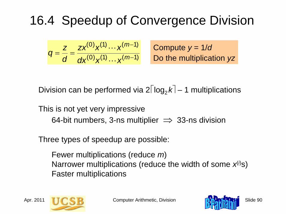
16.4 Speedup of Convergence Division
Division can be performed via 2 ⎡log2k⎤ – 1 multiplications
This is not yet very impressive64-bit numbers, 3-ns multiplier ⇒ 33-ns division
Three types of speedup are possible:
Fewer multiplications (reduce m) Narrower multiplications (reduce the width of some x(i)s)Faster multiplications
)1()1()0(
)1()1()0(
−
−== m
m
xxdxxxzx
dzq
L
L Compute y = 1/d Do the multiplication yz
Apr. 2011 Computer Arithmetic, Division Slide 91
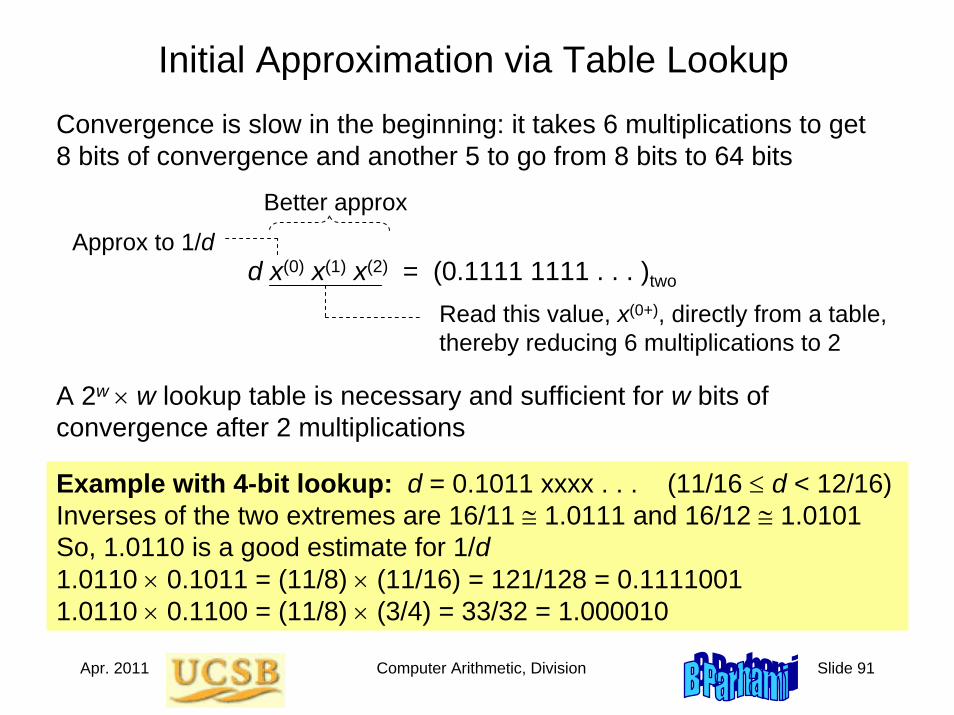
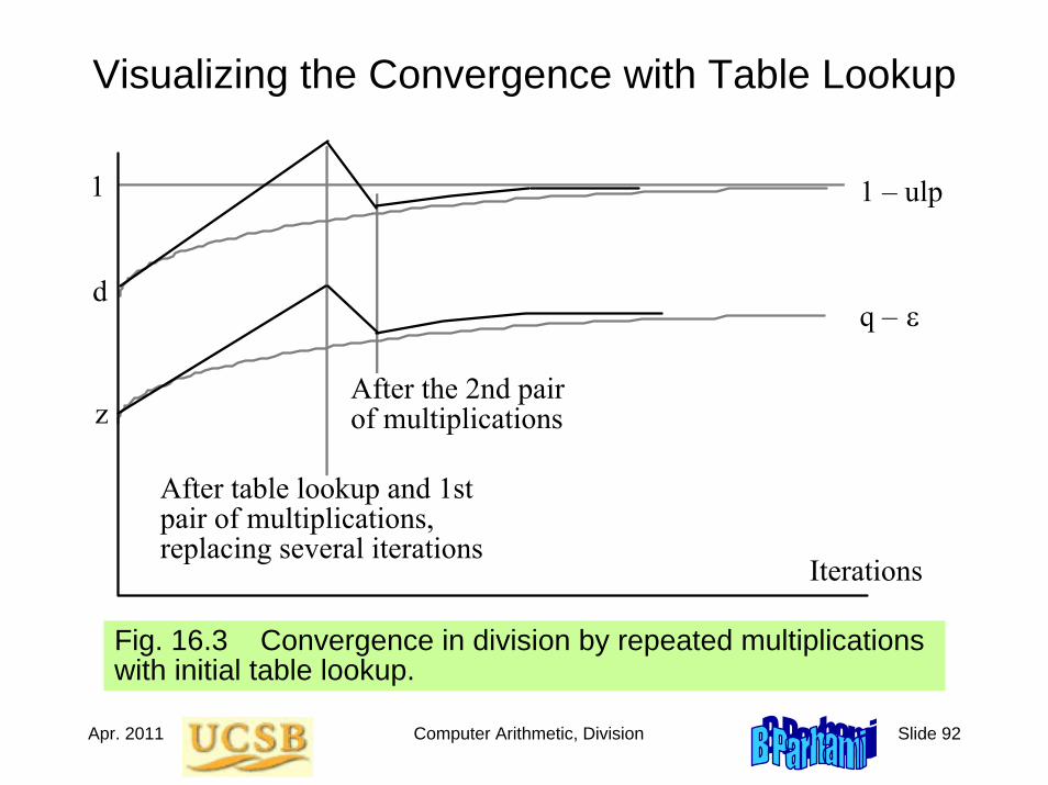
Initial Approximation via Table LookupConvergence is slow in the beginning: it takes 6 multiplications to get 8 bits of convergence and another 5 to go from 8 bits to 64 bits
d x(0) x(1) x(2) = (0.1111 1111 . . . )two
Approx to 1/d
Better approx
Read this value, x(0+), directly from a table, thereby reducing 6 multiplications to 2
A 2w × w lookup table is necessary and sufficient for w bits of convergence after 2 multiplications
Example with 4-bit lookup: d = 0.1011 xxxx . . . (11/16 ≤ d < 12/16)Inverses of the two extremes are 16/11 ≅ 1.0111 and 16/12 ≅ 1.0101 So, 1.0110 is a good estimate for 1/d1.0110 × 0.1011 = (11/8) × (11/16) = 121/128 = 0.1111001 1.0110 × 0.1100 = (11/8) × (3/4) = 33/32 = 1.000010
Apr. 2011 Computer Arithmetic, Division Slide 92
Visualizing the Convergence with Table Lookup
Fig. 16.3 Convergence in division by repeated multiplications with initial table lookup.
1 1 – ulp
d
z
q –
Iterations
After table lookup and 1st pair of multiplications, replacing several iterations
After the 2nd pair of multiplications
ε
Apr. 2011 Computer Arithmetic, Division Slide 93
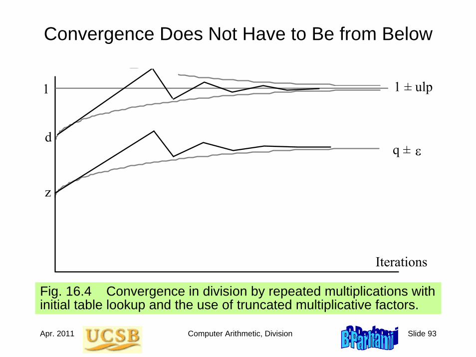
Convergence Does Not Have to Be from Below
Fig. 16.4 Convergence in division by repeated multiplications with initial table lookup and the use of truncated multiplicative factors.
1 1 ± ulp
d
z
q ±
Iterations
ε

Apr. 2011 Computer Arithmetic, Division Slide 94
Using Truncated Multiplicative Factors
Fig. 16.4 One step in convergence division with truncated multiplicative factors.
1
Approximate iteration
Precise iteration
B
A
i + 1 i
Iteration
(x (i+1)
d x (0) x (1) x (i) ... x (i+1)
) T
d x (0) x (1) x (i) ...
d x (0) x (1) x (i) ...
< 2 −a
Example (64-bit multiplication)Initial step: Table of size 256 × 8 = 2K bitsMiddle steps: Multiplication pairs, with 9-, 17-, and 33-bit multipliersFinal step: Full 64 × 64 multiplication
Problem 16.9aA truncated denominator d (i), with aidentical leading bits and b extra bits (b ≤ a), leads to a new denominator d (i+1) with a + b identical leading bits
Apr. 2011 Computer Arithmetic, Division Slide 95
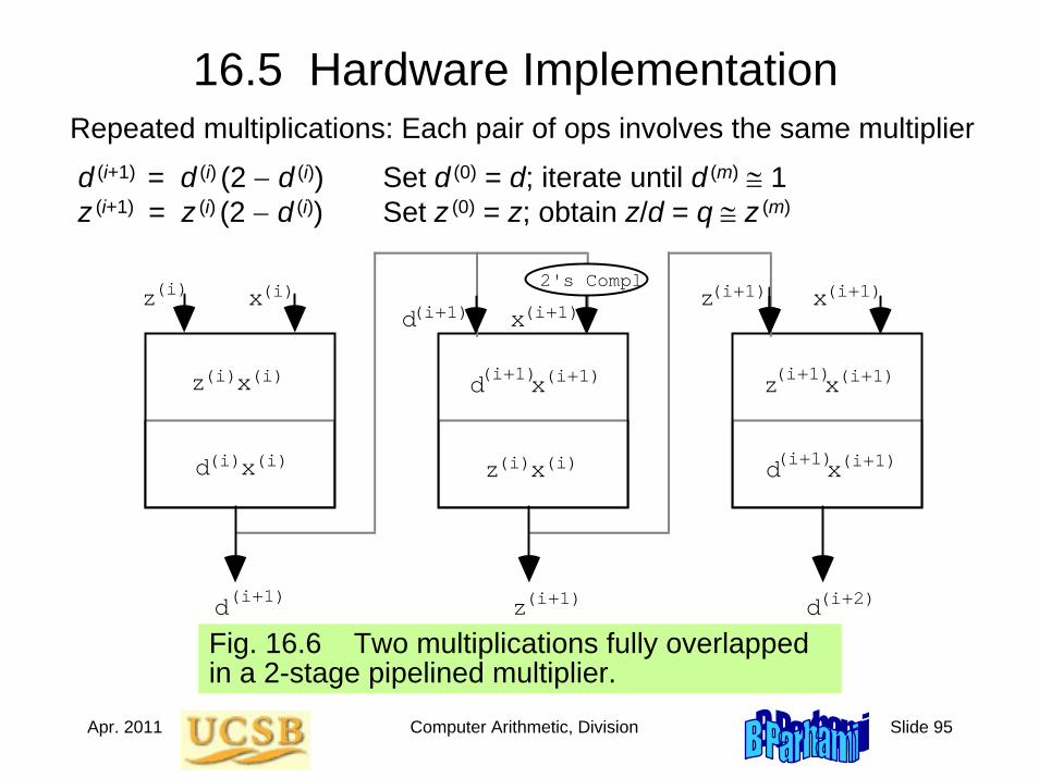
16.5 Hardware ImplementationRepeated multiplications: Each pair of ops involves the same multiplier
d (i+1) = d (i) (2 − d (i)) Set d (0) = d; iterate until d (m) ≅ 1z (i+1) = z (i) (2 − d (i)) Set z (0) = z; obtain z/d = q ≅ z (m)
Fig. 16.6 Two multiplications fully overlapped in a 2-stage pipelined multiplier.
z x(i)(i)
d x(i)(i)
x(i)z(i)d(i+1)
d(i+1)
x(i+1)
z x(i)(i)
d x(i+1)(i+1)
z(i+1)
2's Complz(i+1) x(i+1)
z x(i+1)(i+1)
d(i+2)
d x(i+1)(i+1)
Apr. 2011 Computer Arithmetic, Division Slide 96
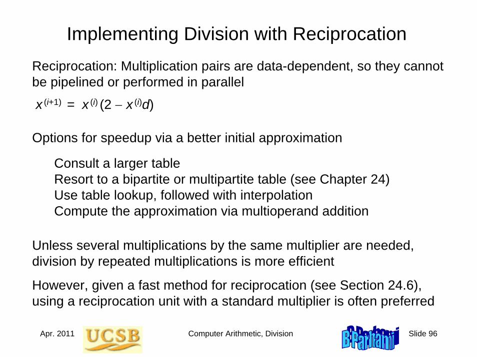
Implementing Division with ReciprocationReciprocation: Multiplication pairs are data-dependent, so they cannot be pipelined or performed in parallel
x (i+1) = x (i) (2 − x (i)d)
Options for speedup via a better initial approximation
Consult a larger tableResort to a bipartite or multipartite table (see Chapter 24) Use table lookup, followed with interpolationCompute the approximation via multioperand addition
Unless several multiplications by the same multiplier are needed, division by repeated multiplications is more efficient
However, given a fast method for reciprocation (see Section 24.6), using a reciprocation unit with a standard multiplier is often preferred
Apr. 2011 Computer Arithmetic, Division Slide 97
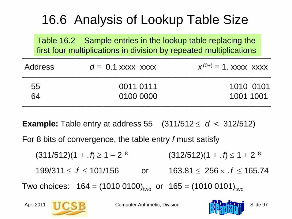
16.6 Analysis of Lookup Table SizeTable 16.2 Sample entries in the lookup table replacing the first four multiplications in division by repeated multiplications
–––––––––––––––––––––––––––––––––––––––––––––––––––––––Address d = 0.1 xxxx xxxx x (0+) = 1. xxxx xxxx
–––––––––––––––––––––––––––––––––––––––––––––––––––––––55 0011 0111 1010 010164 0100 0000 1001 1001
–––––––––––––––––––––––––––––––––––––––––––––––––––––––
Example: Table entry at address 55 (311/512 ≤ d < 312/512)
For 8 bits of convergence, the table entry f must satisfy
(311/512)(1 + . f) ≥ 1 – 2–8 (312/512)(1 + . f) ≤ 1 + 2–8
199/311 ≤ .f ≤ 101/156 or 163.81 ≤ 256 × . f ≤ 165.74
Two choices: 164 = (1010 0100)two or 165 = (1010 0101)two
Apr. 2011 Computer Arithmetic, Division Slide 98
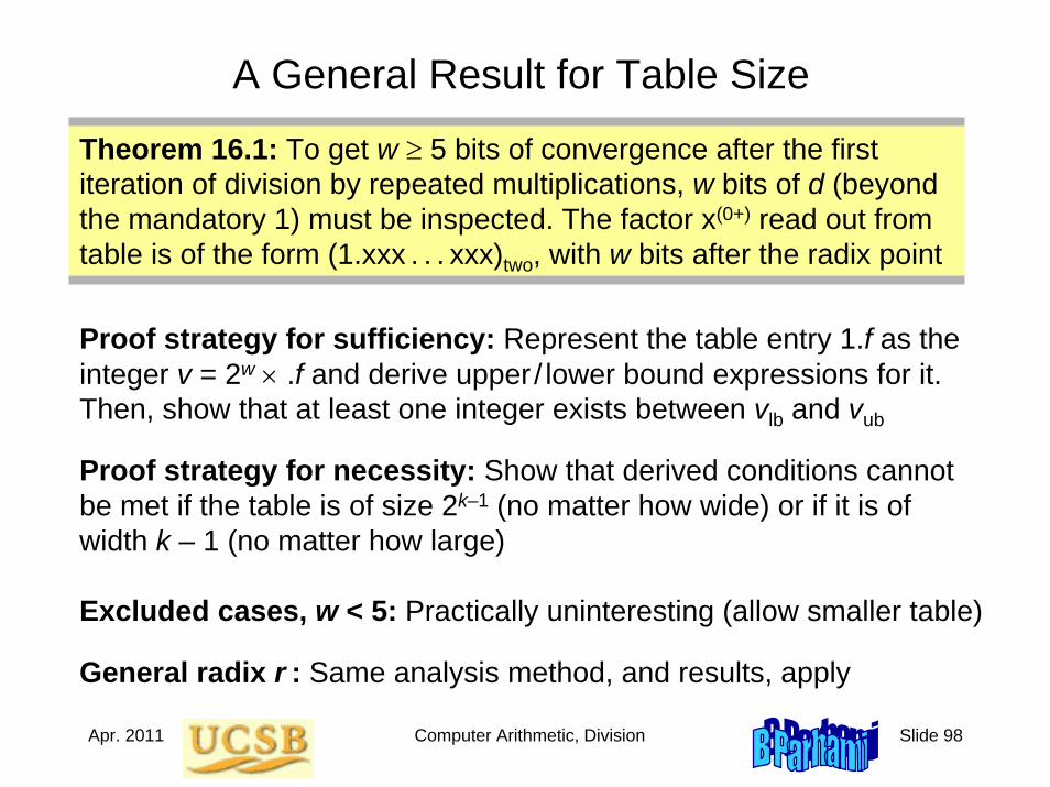
A General Result for Table Size
Proof strategy for sufficiency: Represent the table entry 1.f as the integer v = 2w × .f and derive upper / lower bound expressions for it. Then, show that at least one integer exists between vlb and vub
Theorem 16.1: To get w ≥ 5 bits of convergence after the first iteration of division by repeated multiplications, w bits of d (beyond the mandatory 1) must be inspected. The factor x(0+) read out from table is of the form (1.xxx . . . xxx)two, with w bits after the radix point
Proof strategy for necessity: Show that derived conditions cannot be met if the table is of size 2k–1 (no matter how wide) or if it is of width k – 1 (no matter how large)
Excluded cases, w < 5: Practically uninteresting (allow smaller table)
General radix r : Same analysis method, and results, apply