Computer Graphics MCA-203bvicam.in/sites/default/files/subject/LearningMannuals...MCA-203, Computer Graphics © Bharati Vidyapeeth’s Institute of Computer A pplications and Management,

MCA-203, Computer Graphics

© Bharati Vidyapeeth’s Institute of Computer Applications and Management, New Delhi-63, by Vaishali Joshi, Assistant Professor

U1.1

Computer Graphics

© Bharati Vidyapeeth’s Institute of Computer Applications and Management, New Delhi-63, by Vaishali Joshi, Assistant Professor – Unit 1 1

MCA-203

UNIT-I


Scan Conversion and Transformations

In this unit, we’ll cover the following:

• Graphics Primitives

• Display Devices

• Scan Conversion

Learning Objectives

© Bharati Vidyapeeth’s Institute of Computer Applications and Management, New Delhi-63, by Vaishali Joshi, Assistant Professor – Unit 1

– Point

– Line

– Circle etc.

– Filled-Area Primitives

• Transformations– Two Dimensional (2D)

– Three Dimensional (3D)

3



U1.2

G hi P i iti


Graphics Primitives

We’ll cover the following:• What is Computer Graphics

• Its Application

• What is Pixel

Contents


at s e

• Black & White and Colored images

• Display File

• Frame Buffer

• Aspect Ratio

• Resolution

• Color Models

5

• Refers to creation, storage and manipulation of pictures and drawings using a digital computer

• Effective tool for presenting information

What is Computer Graphics


• It increases the communication bandwidth between humans and machines

6



U1.3

• Science & engineering

• Medicine

• Business

• Government

Applications of Computer Graphics


• Art

• Entertainment

• Advertising

• Education and training

7


• Its Application

• What is Pixel

Contents


at s e


• Display File

• Frame Buffer

• Aspect Ratio

• Resolution

• Color Models

8


• Its Application

• What is Pixel

Contents


at s e


• Display File

• Frame Buffer

• Aspect Ratio

• Resolution

• Color Models

9



U1.4


• Its Application

• What is Pixel

Contents


What is Pixel


• Display File

• Frame Buffer

• Aspect Ratio

• Resolution

• Color Models

10

Frame Buffers

• A frame buffer may be thought of as computer memory organized as a two-dimensional array with each (x,y) addressable location corresponding to one pixel.

• Bit Planes or Bit Depth is the number of bits corresponding to each pixel


to each pixel.

• A typical frame buffer resolution might be

– 640 x 480 x 8

– 1280 x 1024 x 8

– 1280 x 1024 x 24

11


• Its Application

• What is Pixel

Contents


at s e


• Display File

• Frame Buffer

• Aspect Ratio

• Resolution

• Color Models

12



U1.5


• Its Application

• What is Pixel

Contents


What is Pixel


• Display File

• Frame Buffer

• Aspect Ratio

• Resolution

• Color Models

13

Color Models

There are two most common Color models :

• RGB Color Model (Red-Green-Blue)

Additive model Additive color models use light to display color


Additive color models use light to display color

Colors perceived in additive models are the result oftransmitted light

• CMYK Color Model (Cyan-Magenta-Yellow-blacK)

Subtractive model

subtractive models use printing inks.

Colors perceived in subtractive models are the result of reflected light

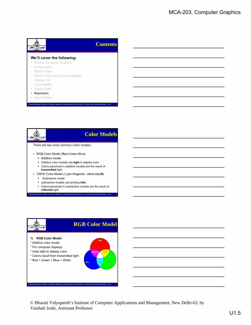
1) RGB Color Model:

* Additive color model.

* For computer displays.

* Uses light to display color.

RGB Color Model


Uses light to display color.

* Colors result from transmitted light.

* Red + Green + Blue = White.



U1.6

2) CMYK Color Model:

* Subtractive color model.

* For printed material.

* Uses ink to display color

CYMK Color Model


Uses ink to display color.

* Colors result from reflected light.

* Cyan + Magenta + Yellow = Black.



• Display Devices

• Scan Conversion

Learning Objectives


– Point

– Line

– Circle etc.




17

Di l D i


Display Devices



U1.7

• Refresh CRT

• Raster Scan Display

• Random Scan Display

• Color CRT Monitors

Contents


– Beam Penetration Method

– Shadow Mask Method

• Flat Panel Displays– Emissive Display

• Plasma Panels

• LED

– Nonemissie Display

• LCD

19

Base

Focusing system

Vertical deflecting plates Phosphor

coated screen

Refresh CRT


Connector Pins

Electron gun Horizontal

deflecting plates

Electron beam

Raster Scan Displays

• The most common type of monitor employing a CRT is raster scan display. • In Raster scan display the electron beam is swept across the screen one row at a time from top to bottom. • Raster: A rectangular array of points or dots• Pixel: One dot or picture element of the raster. Its intensity


range for pixels depends on capability of the system• Scan line: A row of pixels• Picture elements are stored in a memory called frame buffer• A special memory is used to store the image with scan-out synchronous to the raster. We call this the frame buffer

DisadvantageRaster system produces jagged lines that are plotted as discrete points

21



U1.8

Raster Scan Displays cont..


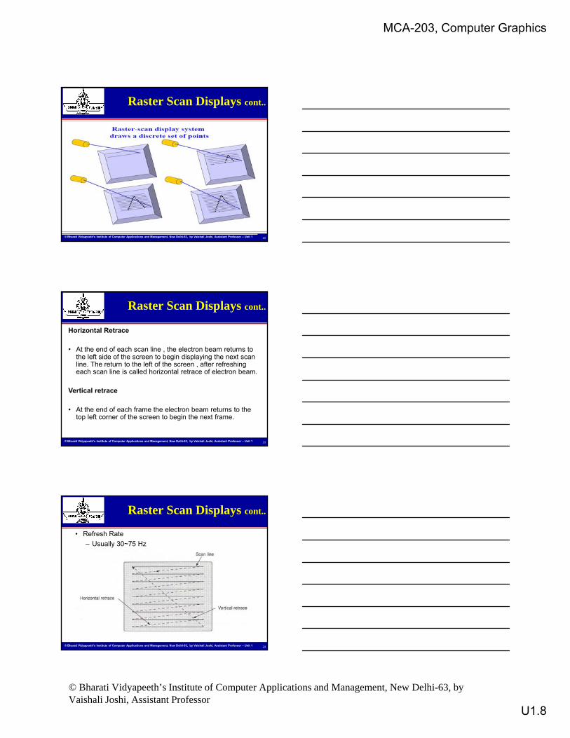
Horizontal Retrace

• At the end of each scan line , the electron beam returns to the left side of the screen to begin displaying the next scan line. The return to the left of the screen , after refreshing



each scan line is called horizontal retrace of electron beam.

Vertical retrace

• At the end of each frame the electron beam returns to the top left corner of the screen to begin the next frame.

23


• Refresh Rate

– Usually 30~75 Hz




U1.9


123456789

1011

Interlacing


1213141516171819202122

•First, all points on the even-numbered (solid) scan-lines are displayed•Then all points along odd-numbered (dashed) lines are displayed

Random Scan Display

•The electron beam is directed only to the parts of the screen where a picture is to be drawn.

•Picture definition is stored as a set of line drawing commands in an area of memory referred to as refresh display file.


•To display a specified picture ,the system cycles through a set of commands in the display file , drawing each component line after processing all lines drawing commands the s/m cycle back to the first line command in the list.

AdvantageHas high resolution since picture definition is stored as line drawing commands

26

Random Scan Display cont...




U1.10

2 Basic Techniques for Color Display

Color CRT Monitors


Beam Penetration Method

Shadow Mask Method

28

Beam-Penetration Method

•Used with random scan monitors

•The screen has two layers of phosphor: usually red and green

•The displayed color depends on how far the electron beam penetrates through the two layers


penetrates through the two layers.

•A beam of slow electrons excites only the outer of the red layer, a beam of fast electrons penetrates through the red layer and excites the inner green layer, and at intermediate beam speeds, combinations of the two colors are emitted to show other colors (yellow & orange)

29

Shadow-Mask Method

– Used with raster scan monitors

– Three electron guns

– A metal shadow mask to differentiate the beams




U1.11

•The Shadow mask in the previous image is known as the delta‐delta shadow‐mask.

•The 3 electron beams are deflected and focused as a group onto the shadow mask, which contains a series of holes aligned with the phosphor‐dot patterns.

Th 3 b h h h l i h h d k d

Shadow-Mask Method cont..


•The 3 beams pass through a hole in the shadow mask and activate a dot triangle, which appears as a small color spot on the screen.

•A second arrangement of the 3 electron guns is in‐line

Where the corresponding red‐green‐blue color dots on the screen are aligned along one scan – line instead of a triangular pattern.

31

Controlling Colors in shadow mask

•Different colors can be obtained by varying the intensity levels of the three electron beams.

•Example: Simply turning off the red and green guns, we get only the color coming from the blue phosphor.


•Yellow = Green + Red

•Magenta = Blue + Red

•Cyan = Blue + Green

•White is produced when all the 3 guns possess equal amount of intensity.

32

• Refresh CRT

• Raster Scan Display

• Random Scan Display

• Color CRT Monitors

Contents


– Beam Penetration Method

– Shadow Mask Method

• Flat Panel Displays– Emissive Display

• Plasma Panels

• LED

– Nonemissie Display

• LCD

33



U1.12



• Display Devices

• Scan Conversion

Learning Objectives


– Point

– Line

– Circle etc.




34

S C i


Scan Conversion

Scan Conversion

Output Primitives

• Basic geometric structures used to describe scenes.

•Can be grouped into more complex structures

•Example : Point, straight line segments, circles and other conic sections polygon color areas and character strings


sections, polygon color areas and character strings

•Construct the vector picture

Rasterization

The process of determining the appropriate pixels for representing picture or graphic object

Scan conversion

It is the final step of rasterization . It converts picture definition into a set of pixel-intensity values for storage in the frame buffer.

36



U1.13

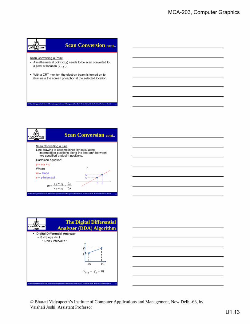
Scan Converting a Point

• A mathematical point (x,y) needs to be scan converted to a pixel at location (x´, y´).

Scan Conversion cont..


• With a CRT monitor, the electron beam is turned on to illuminate the screen phosphor at the selected location.

37

Scan Converting a LineLine drawing is accomplished by calculating

intermediate positions along the line path between two specified endpoint positions.

Cartesian equation:

Scan Conversion cont..


y = mx + c

Where

m – slope

c – y-intercept

x1

y1

x2

y2

x

y

xx

yym

12

12

38

The Digital Differential Analyzer (DDA) Algorithm

• Digital Differential Analyzer– 0 < Slope <= 1

• Unit x interval = 1

y2


x1

y1

x2

myy kk 1



U1.14

The DDA Algorithm cont..



– Slope > 1• Unit y interval = 1

y2


• Unit y interval = 1

x1

y1

x2

mxx kk

11





y1



– -1 <= Slope < 0• Unit x interval = -1

myy kk 1

x1

y2

x2





y2



– -1 <= Slope < 0• Unit x interval = -1

– Slope < -1• Unit y interval = -1 m

xx kk

11

x1

y1

x2



U1.15

DDA ALGORITHM

1. START 2. Get the values of the starting and ending co-ordinates i.e. ,(xa,ya) and (xb,yb). 3. Find the value of slope m



m=dy/dx=((yb-ya)/(xb-xa)) 4. If ImI ≤ 1 then Δx=1,Δy=mΔx

xk+1=xk+1,yk+1=yk+m 5. If ImI ≥ 1 then Δy=1,Δx=Δy/m

xk+1=xk+1/m,yk+1=yk+1 6. STOP


Desired line

(x +1 round(y +m))


(xi,round(yi))

(xi,yi)

(xi+1,round(yi+m))

(xi+1,yi+m)

44

Example (DDA)

31

1

131 1

10 1

ii

ii

yyxx

mxy

x y round(y)

0 1 11 4/3 1

8

7

y


1 4/3 12 5/3 23 2 24 7/3 25 8/3 36 3 37 10/3 38 11/3 4

6

5

4

3

2

1

0

0 1 2 3 4 5 6 7 8 x

45



U1.16

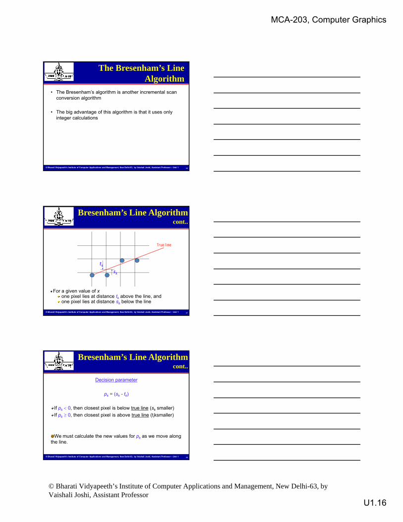
• The Bresenham’s algorithm is another incremental scan conversion algorithm

• The big advantage of this algorithm is that it uses only i t l l ti

The Bresenham’s Line Algorithm


integer calculations

46

Bresenham’s Line Algorithm cont..

True line


For a given value of xone pixel lies at distance tk above the line, andone pixel lies at distance sk below the line

sk

tk

47

Decision parameter

pk = (sk - tk)



If pk 0, then closest pixel is below true line (sk smaller)

If pk 0, then closest pixel is above true line (tiksmaller)

We must calculate the new values for pk as we move along the line.

48



U1.17

Algorithm1. Input line end points2. Load (x0,y0) to plot the first point.3. Calculate dx,dy, 2dy and 2dy-2dx and obtain the starting

value of the decision parameter as p0=2dy-dx



4. At each xk along the line, starting at k=0, perform the following test if pk <0, the next point plot is (xk+1, yk) and

pk+1=pk+2dyOther wise, the next point to pot is (xk+1, yk+1) and

pk+1=pk+2dy-2dx5. Repeat step-4 dx times.

49

Example (Bresenham’s Line Algorithm )

19

18

17

Draw a line from (20,10) to (30,18)dx = 10 dy = 8 initial decision d0 = 2dy – dx = 6Also 2dy = 16, 2(dy – dx) = ‐4

k pk (xk+1,yk+1)

0 6 (21,11) 1 2 (22 12)


17

16

15

14

13

12

11

10

20 21 22 23 24 25 26 27 28 29 30 31 32

1 2 (22,12) 2 -2 (23,12) 3 14 (24,13) 4 10 (25,14) 5 6 (26,15) 6 2 (27,16) 7 -2 (28,16) 8 14 (29,17) 9 10 (30,18)

50

Special cases•Special cases can be handled separately

– Horizontal lines (y = 0)

– Vertical lines (x = 0)



– Diagonal lines (|x| = |y|)

•directly into the frame-buffer without processing them through the line-plotting algorithms.

51



U1.18

Circle Equations Circle Equations ((Cartesian form)

The equation for a circle is:where r is the radius of the circleSo, we can write a simple circle drawing algorithm by solving the equation for y at unit x intervals using:

222 ryx

22 xry


y

x x

y

r 2 2,P x r x

xry

52

Circle Algorithms

•Use 8-fold symmetry and only compute pixel positions for the 45° sector.

(x, y)(‐x, y)


45° (y, x)

(y, ‐x)

(x, ‐y)(‐x, ‐y)

(‐y, x)

(‐y, ‐x)

53

Bresenham’s Circle Algorithm

General PrincipleGeneral Principle

•The circle function:

Consider only 45° ≤ ≤ 90°


•and

2 2 2( , )circlef x y x y r

if (x,y) is inside the circle boundary

if (x,y) is on the circle boundary

if (x,y) is outside the circle boundary

0

( , ) 0

0circlef x y

54



U1.19

p1 p3

p2

D(sk)D(tk)

yk

yk‐ 1

Bresenham’s Circle Algorithm Cont..


After point p1, do we choose p2 or p3?

xk xk+ 1

r

55

MID-POINT CIRCLE ALGORITHM

1. Input radius r and circle centre (xc, yc), then set the coordinates for the first point on the circumference of a circle centred on the origin as:

),0(),( 00 ryx

Mid-point Circle Algorithm


2. Calculate the initial value of the decision parameter as:

3. Starting with k = 0 at each position xk, perform the following test. If pk < 0, the next point along the circle centred on (0, 0) is (xk+1, yk) and:

12 11 kkk xpp

),0(),( 00 ryx

rp 45

0

56

Otherwise the next point along the circle is (xk+1, yk-1) and:

4. Determine symmetry points in the other seven octants

111 212 kkkk yxpp

Mid-point Circle AlgorithmCont..


5. Move each calculated pixel position (x, y) onto the circular path centred at (xc, yc) to plot the coordinate values:

6. Repeat steps 3 to 5 until x >= y

cxxx cyyy

57



U1.20

Example (Mid Point Circle Algorithm)

10

9

8

r = 10

p0 = 1 – r = ‐9 (if r is integer round p0 = 5/4 – r to integer)

Initial point (x0, y0) = (0, 10)

i pi xi+1, yi+1 2xi+1

2yi+1

0 9 (1 10) 2 20


7

6

5

4

3

2

1

0

0 1 2 3 4 5 6 7 8 9 10

0 -9 (1, 10) 2 20

1 -6 (2, 10) 4 20

2 -1 (3, 10) 6 20

3 6 (4, 9) 8 18

4 -3 (5, 9) 10 18

5 8 (6, 8) 12 16

6 5 (7, 7) 14 14

58

Ellipse-Generating Algorithms

•Ellipse – A modified circle whose radius varies from a maximum value in one direction (major axis) to a minimum value in the perpendicular direction (minor axis).


P=(x,y)F1

F2

d1

d2

The sum of the two distances d1 and d2, between the fixed positions F1 and F2 (called the foci of the ellipse) to any point P on the ellipse, is the same value, i.e.

d1 + d2 = constant

59

ry

rx

Minor

Major

Ellipse Properties

•Expressing distances d1 and d2 in terms of the focal coordinates F1 = (x1, x2) and F2 = (x2, y2), we have:

2 2 2 21 1 2 2( ) ( ) ( ) ( ) constantx x y y x x y y

Ellipse-Generating Algorithms Cont..


•Cartesian coordinates:

ry

rx

22

1c c

x y

x x y y

r r

60



U1.21

•Symmetry between quadrants

•Not symmetric between the two octants of a quadrant

•Thus, we must calculate pixel positions along the elliptical arc through one quadrant and then we obtain positions in the remaining 3 quadrants by symmetry



positions in the remaining 3 quadrants by symmetry

(x, y)(‐x, y)

(x, ‐y)(‐x, ‐y)

rx

ry

61

•Decision parameter:

2 2 2 2 2 2( , )ellipse y x x yf x y r x r y r r

0 i f ( , ) i s in s id e th e e llip s e

( , ) 0 i f ( , ) i s o n th e e llip s ee l l ip se

x y

f x y x y



1

Slope = ‐1

rx

ry 2

0 i f ( , ) i s o u ts id e th e e llip s ep

x y

2

2

2

2y

x

r xdySlope

dx r y

62

Midpoint Ellipse Algorithm

1. Input rx, ry, and ellipse center (xc, yc), and obtain the first point on an ellipse centered on the origin as

(x0, y0) = (0, ry)2. Calculate the initial parameter in region 1 as

2 2 210 41 y x y xp r r r r


3. At each xi position, starting at i = 0, if p1i < 0, the next point along the ellipse centered on (0, 0) is (xi + 1, yi) and

otherwise, the next point is (xi + 1, yi – 1) and

and continue until

2 21 11 1 2i i y i yp p r x r

2 2 21 1 11 1 2 2i i y i x i yp p r x r y r

2 22 2y xr x r y

63



U1.22

4. (x0, y0) is the last position calculated in region 1. Calculate the initial parameter in region 2 as

5. At each yi position, starting at i = 0, if p2i > 0, the next point along the ellipse centered on (0, 0) is (xi, yi – 1) and

2 2 2 2 2 210 0 022 ( ) ( 1)y x x yp r x r y r r

2 22 2 2p p r y r

Midpoint Ellipse Algorithm cont..


otherwise, the next point is (xi + 1, yi – 1) and

Use the same incremental calculations as in region 1. Continue until y = 0.

6. For both regions determine symmetry points in the other three quadrants.

7. Move each calculated pixel position (x, y) onto the elliptical path centered on (xc, yc) and plot the coordinate values

x = x + xc , y = y + yc

1 12 2 2i i x i xp p r y r

2 2 21 1 12 2 2 2i i y i x i xp p r x r y r

64

Example ((Midpoint Ellipse Algorithm)

rx = 8 , ry = 6

2ry2x = 0 (with increment 2ry

2 = 72)

2rx2y = 2rx

2ry (with increment ‐2rx2 = ‐128)

Region 1Region 1

(x0, y0) = (0, 6)2 2 21

0 41 332y x y xp r r r r


i pi xi+1, yi+1 2ry2xi+1 2rx

2yi+1

0 -332 (1, 6) 72 768

1 -224 (2, 6) 144 768

2 -44 (3, 6) 216 768

3 208 (4, 5) 288 640

4 -108 (5, 5) 360 640

5 288 (6, 4) 432 512

6 244 (7, 3) 504 384

Move out of region 1 since2ry

2x > 2rx2y

65

Example ((Midpoint Ellipse Algorithm) cont..

i p x y 2r 2x 2r 2y

Region 2Region 2

(x0, y0) = (7, 3) (Last position in region 1)1

0 22 (7 ,2) 151ellipsep f Stop at y = 0


6

5

4

3

2

1

0

0 1 2 3 4 5 6 7 8

i pi xi+1, yi+1 2ry xi+1 2rx yi+1

0 -151 (8, 2) 576 256

1 233 (8, 1) 576 128

2 745 (8, 0) - -

66



U1.23

Filled Area Primitives

•Polyline - A chain of connected line segments. •Polygon - When starting point and terminal point of any polyline is same, i,e when polyline is closed then it is called polygon


Two Basic approaches to Area-Filling –•Scan-line Method

Determine the overlap intervals for scan lines that cross the area. It is typically used in general graphics packages to fill polygons, circles, ellipses

Filled Area Primitives cont..


•Fill Method Start from a given interior position and paint outward from this point until we encounter the specified boundary conditions. Useful with more complex boundaries and in interactive painting systems.

1. Boundary Fill2. Flood Fill





U1.24


Boundary – Fill Algorithms

Start at a point inside a region and paint the interior outward toward the boundary. If the boundary is specified in a single color, the fill algorithm proceeds outward pixel by pixel until the boundary color is encountered


pixel until the boundary color is encountered.

It is useful in interactive painting packages, where interior points are easily selected.

The inputs of the this algorithm are:• Coordinates of the interior point (x, y) • Fill Color• Boundary Color


Sometimes we want to fill in (or recolor) an area that is not defined within a single color boundary. We can paint such areas by replacing a specified interior color instead of searching for a


gboundary color value. This approach is called a flood-fill algorithm.

We start from a specified interior point (x, y) and reassign all pixel values that are currently set to a given interior color with the desired fill color.



• Display Devices

• Scan Conversion

Learning Objectives


– Point

– Line

– Circle etc.




72



U1.25

2D T f ti


2D Transformations

2D Transformation

Given a 2D object, transformation is to change the object’s Position (translation)

Size (scaling)


Orientation (rotation)

Shapes (shear)

Reflection

74

•A translation moves all points in an object along the same straight-line path to new positions.

•The path is represented by a vector, called the translation or

?

Translation


,shift vector.

•We can write the components:

p'x = px + txp'y = py + ty

•or in matrix form:

P' = P + T

tx

ty

(2, 2)= 6

=4

x’

Y’

x

y

txty

= +

75



U1.26

Scaling

• Scaling changes the size of an object and involves two scale factors, Sx and Sy for the x- and y- coordinates respectively.

• Scales are about the origin.

P’


• We can write the components:p'x = sx • px

p'y = sy • py

or in matrix form:P' = S • P

Scale matrix as:

y

x

s

sS

0

0

P

76

Scaling cont..

• If the scale factors are in between 0 and 1 the points will be moved closer to the origin the object will be smaller.

•Example :


P(2, 5)

P’

•P(2, 5), Sx = 0.5, Sy = 0.5•Find P’ ?

77

• If the scale factors are in between 0 and 1 the points will be moved closer to the origin the object will be smaller.

• Example :•P(2 5) Sx = 0 5 Sy = 0 5

P’

Scaling cont..


P(2, 5)

P’

P(2, 5), Sx 0.5, Sy 0.5•Find P’ ?

•If the scale factors are larger than 1 the points will be moved away from the origin the object will be larger.• Example :

•P(2, 5), Sx = 2, Sy = 2•Find P’ ?

78



U1.27

• If the scale factors are the same, Sx = Sy uniform scaling• Only change in size (as previous example)

P’

Scaling cont..


P(1, 2)

•If Sx Sy differential scaling.•Change in size and shape•Example : square rectangle

•P(1, 3), Sx = 2, Sy = 5 , P’ ?

What does scaling by 1 do?

What is that matrix called?

What does scaling by a negative value do?

79

Rotation

•A rotation repositions all points in an object along a circular path in the plane centered at the pivot point. P’


•First, we’ll assume the pivot is at the origin.

P

80

Rotation cont..

P’(x’, y’)

• Review Trigonometry

=> cos = x/r , sin = y/r

• x = r. cos , y = r.sin => cos (+ ) = x’/r

•x’ = r cos (+ )


P(x,y)

x

yr

x’

y’

r•x = r. cos (+ )

•x’ = r.coscos -r.sinsin•x’ = x.cos – y.sin =>sin (+ ) = y’/r

y’ = r. sin (+ )

•y’ = r.cossin + r.sincos•y’ = x.sin + y.cos

Identity of Trigonometry

81



U1.28

• We can write the components:

p'x = px cos – py sin p'y = px sin + py cos

P’(x’, y’)

Rotation cont..


• or in matrix form:

P' = R • P

• can be clockwise (-ve) or counterclockwise (+ve as our example).

• Rotation matrix

P(x,y)

x

yr

x’

y’

cossin

sincosR

82

y y

x

x

w

Homogeneous Coordinates


•Let’s move our problem into 3D.

•Let point (x, y) in 2D be represented by point (x, y, 1) in the new space.

•Scaling our new point by any value a puts us somewhere along a particular line: (ax, ay, a).

•A point in 2D can be represented in many ways in the new space.

•(2, 4) ---------- (8, 16, 4) or (6, 12, 3) or (2, 4, 1) or etc.83

• We can always map back to the original 2D point by dividing by the last coordinate

• (15, 6, 3) --- (5, 2).

• (60, 40, 10) - ?.

Homogeneous Coordinates cont..


• Why do we use 1 for the last coordinate?

• The fact that all the points along each line can be mapped back to the same point in 2D gives this coordinate system its name – homogeneous coordinates.

84



U1.29

Homogeneous Coordinates cont..

•Translation

R t ti

1100

10

01

1

y

x

t

t

y

x

y

x

0sincos xx


•Rotation

•Scaling

1100

0cossin

0sincos

1

y

x

y

x

1100

00

00

1

y

x

s

s

y

x

y

x

85

x

y y

x

y

Reflection


x

x

x

1 0 0

0 1 0

0 0 1

1 0 0

0 1 0

0 0 1

1 0 0

0 1 0

0 0 1

86

y x y x

Reflection cont..


0 1 0

1 0 0

0 0 1

0 1 0

1 0 0

0 0 1

87



U1.30

The Shear Transformation cause the image to slant. X-Shear maintains the y-coordinates but changes x values which cause the vertical line to tilt left or right. The Y-shear preserves all the x coordinate values but shifts the y coordinate.

Shear Transformation


Transformations between coordinate systems

yThis is done in two steps :1. Translate the origin (x0,y0) of x’y’ y’system to origin of xy system2 Rotate the x’ axis onto the x-axis x’


2. Rotate the x axis onto the x axis xy0 θ

x0 xMxyx’y’ = R(-θ) . T(-x0,-y0)

Affine Transformations

Properties of affine transformations :

•Each of the transformed coordinates x’ and y’ is a linear function of the original coordinates x and y


•Parallel lines are transformed into parallel lines

•Finite points map to finite points

•An affine transformation involving only rotation, translation and reflection preserves angles and lengths, as well as parallel lines



U1.31

3D T f ti


3D Transformations

Everything we describe in our 3D worlds, e.g. vertices to describe objects, speed of objects, forces on objects, will be defined by

3D VECTORS i.e. triplets of 3 real values V = (x, y, z)

3D Euclidean Coordinate System( 3D C t i C di t S t )

3D Concepts


(or 3D Cartesian Coordinate System)

x

y

z

• To move/animate objects or to change the camera’s position we have to transform the vertices defining our objects.

• Homogeneous coordinates: (x,y,z)=(hx,hy,hz,h)

Basic 3D Transformations


• Transformations are now represented as 4x4 matrices

• Basic 3D transformations are – Translation– Rotation– Scaling



U1.32

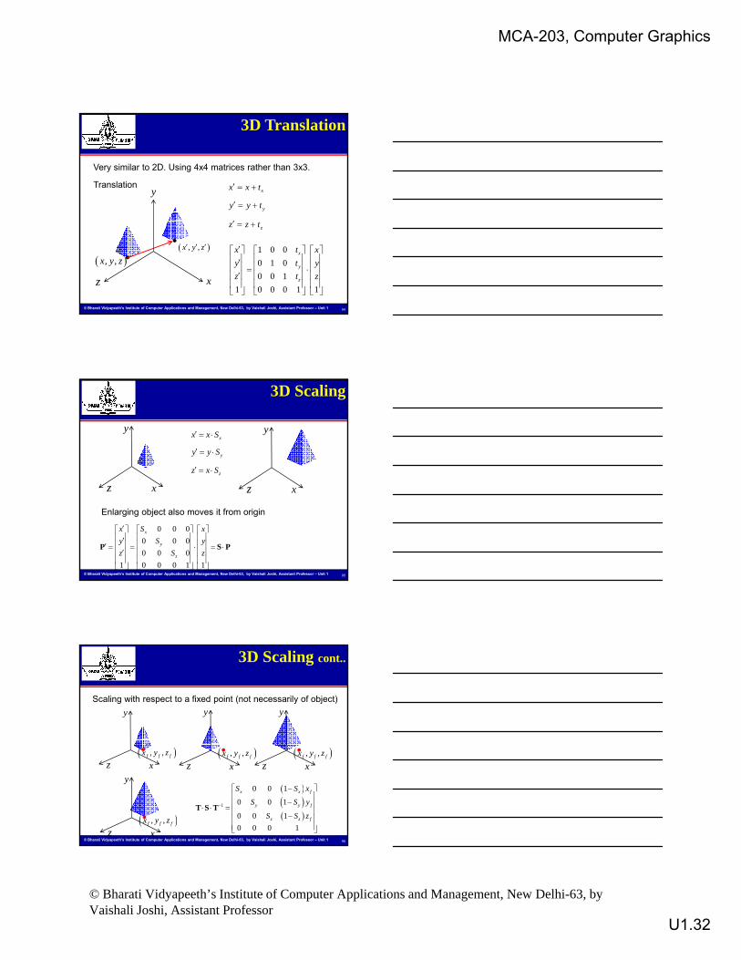
3D Translation

Translationy x

y

x x t

y y t

Very similar to 2D. Using 4x4 matrices rather than 3x3.


, ,x y z

, ,x y z

xz

zz z t

1 0 0

0 1 0

0 0 1

1 0 0 0 1 1

x

y

z

x t x

y t y

z t z

94

y yx

y

z

x x S

y y S

z x S

3D Scaling


xz xz

Enlarging object also moves it from origin

0 0 0

0 0 0

0 0 0

1 0 0 0 1 1

x

y

z

x S x

y S y

z S z

P S P

95

y

Scaling with respect to a fixed point (not necessarily of object)

y y

3D Scaling cont..


, ,f f fx y z

xz , ,f f fx y z

xz , ,f f fx y z

xz

, ,f f fx y z

x

y

z

1

0 0 1

0 0 1

0 0 1

0 0 0 1

x x f

y y f

z z f

S S x

S S y

S S z

T S T

96



U1.33

3D Rotation

• Coordinate-Axes Rotations

– X-axis rotation

– Y-axis rotation

– Z-axis rotation


• General 3D Rotations

– Rotation about an axis that is parallel to one of the coordinate axes

– Rotation about an arbitrary axis

• Positive Rotations are defined as follows:

Axis of rotation is Direction of positive rotation is

• x y to z

• y z to x

z x to y

3D Rotation

y


• z x to y

x

z

Right-hand rule for rotations by positive θ

3D Rotation cont..

Z-Axis Rotation X-Axis Rotation Y-Axis Rotation

0100

00cossin

00sincos

'

'

'

y

x

y

x

0i0

0sincos0

0001

'

'

'

y

x

y

x

00i

0010

0sin0cos

'

'

'

y

x

y

x


11000

0100

1

' zz

z

y

x

11000

0cossin0

1

' zz

11000

0cos0sin

1

' zz

z

y

xz

y

x



U1.34

• Rotation about an Axis that is Parallel to One of the Coordinate Axes– Translate the object so that the rotation axis

coincides with the parallel coordinate axis– Perform the specified rotation about that axis

T l t th bj t th t th t ti i i

General 3D Rotation


– Translate the object so that the rotation axis is moved back to its original position

3D Reflections

Reflection

Reflection relative to xy plane.


1 0 0 00 1 0 00 0 -1 00 0 0 1

x y z 1=x’ y’ z’ 1

Shearing

Z-axis shear

-Where a and b are the shear factors for x and y respectively

3D shears


1 0 0 00 1 0 0a b 1 00 0 0 1

x y z 1=x’ y’ z’ 1



U1.35

In this unit we discuss scan conversion for Point, Line, Circle and ellipse. Along with C Programs for the Scan conversion.

Conclusion


Secondly we under stands the 2D and 3D transformation with some examples.

103

Circles and Ellipses can be efficiently and accurately scan converted using midpoint methods and taking curve symmetry into account.

Summary


The basic geometric transformation are translation, rotation and scaling. Translation moves an object in a Straight line path from one position to another. Rotation movers an object from one position to another in a circular path around a specific rotation point. Scaling Changes the dimensions of an object relative to a specified fixed point.

104

Short answer type QuestionsQ1. Discuss Midpoint Circle Drawing algorithm with the help of an example.Q2. Discuss Bresenham’s algorithm for Scan converting a Line

Review Questions


Line.Q3. Discuss 2D Translation and Scaling with examples.Q4. Compute the intermediate prints on the line drawn from (0, 0) to (5, 10) using DDA algorithm.Q5. What is scan conversion?Q6. What do you mean by Composite transformations? Explain with the help of an example.

105



U1.36

Long answer type QuestionsQ1. Explain various 2D transformation with examplesQ2. Explain various 3D transformation with examplesQ3. Derive the 2D rotational transformation matrix.Q4.What do you mean by rotation in 3D.

Review Questions cont..


y yQ5.Find the matrix that represents rotation of an object by 30 degree about origin in 2D.Q6.Find the transformation that scales (with respect to origin)bya) ‘a’ units in the X-direction.b) ‘b’ units in the Y-direction and c) Simultaneously ‘a’ units in the X-direction and ‘b’ units

in the Y-direction.106

[1]. Donnald Hearn and M. Pauline Baker, “Computer Graphics”, PHI.

[2]. Foley James D, “Computer Graphics”, AW 2nd Ed.

Suggested Reading / References


Ed.

[3]. Rogers, “Procedural Element of Computer Graphics”, McGraw Hill.

[4]. Newman and Sproul, “Principal of to Interactive Computer Graphics”, McGraw Hill.

107

Documents

Computer Graphics MCA-203bvicam.in/sites/default/files/subject/LearningMannuals...MCA-203, Computer Graphics © Bharati Vidyapeeth’s Institute of Computer A pplications and Management,