COMPUTER MODELING OF STRUCTURAL INNOVATIONS IN BIOSENSORS

VILNIUS UNIVERSITY

Mantas Puida

COMPUTER MODELING OF STRUCTURAL INNOVATIONS IN BIOSENSORS

Summary of doctoral dissertation Physical Sciences, informatics (09 P)

Vilnius, 2009

The work presented in this doctoral dissertation has been carried out at the

faculty of Mathematics and Informatics of Vilnius University from 2004 to

2009

Scientific supervisor:

prof. habil. dr. Feliksas Ivanauskas (Vilnius University, Physical Sciences,

informatics – 09P)

The dissertation is defended at the Council of Scientific Field of Informatics of

Vilnius University:

Chairman: prof. dr. Romas Baronas (Vilnius University, Physical Sciences, Informatics – 09P)

Members:

prof. habil. dr. Mifodijus Sapagovas (Institute of mathematics and informatics, Physical Sciences, Informatics – 09P) prof. dr. Jurgis Barkauskas (Vilnius University, Physical Sciences, chemistry – 03P) prof. dr. Algimantas Juozapavičius (Vilnius University, Physical Sciences, Informatics – 09P) dr. Remigijus Šimkus (Institute of Biochemistry, Physical Sciences, Physics – 02P)

Official opponents:

prof. dr. Vytautas Kleiza (Kaunas university of technology, Physical Sciences, Informatics – 09P) doc. dr. Rimantas Vaicekauskas (Vilnius university, Physical Sciences, Informatics – 09P)

The thesis defense will take place at 3 p.m. on September 16, 2009, at the Distance Learning Centre of Vilnius University. Address: Šaltinių 1A, LT-03225, Vilnius, Lithuania. The summary of the thesis was mailed on the 1st of August, 2009. The thesis is available at the Library of Institute of Mathematics and Informatics and at the Library of Vilnius University.

VILNIAUS UNIVERSITETAS

Mantas Puida

KOMPIUTERINIS STRUKTŪRINIŲ INOVACIJŲ BIOJUTIKLIUOSE MODELIAVIMAS

Daktaro disertacija Fiziniai mokslai, informatika (09 P)

Vilnius, 2009

Disertacija rengta 2004–2009 metais Vilniaus universitete

Mokslinis vadovas:

prof. habil. dr. Feliksas Ivanauskas (Vilniaus universitetas, fiziniai mokslai,

informatika – 09P)

Disertacija ginama Vilniaus universiteto Informatikos mokslo krypties taryboje:

Pirmininkas: prof. dr. Romas Baronas (Vilniaus universitetas, fiziniai mokslai, informatika– 09 P)

Nariai:

prof. habil. dr. Mifodijus Sapagovas (Matematikos ir informatikos institutas, fiziniai mokslai, informatika – 09P) prof. dr. Jurgis Barkauskas (Vilniaus universitetas, fiziniai mokslai, chemija – 03P) prof. dr. Algimantas Juozapavičius (Vilniaus universitetas, fiziniai mokslai, informatika – 09P) dr. Remigijus Šimkus (Biochemijos institutas, fiziniai mokslai, fizika – 02P)

Oponentai:

prof. dr. Vytautas Kleiza (Kauno technologijos universitetas, fiziniai mokslai, informatika – 09 P) doc. dr. Rimantas Vaicekauskas (Vilniaus universitetas, fiziniai mokslai, informatika – 09P)

Disertacija bus ginama viešame Informatikos mokslo krypties tarybos pos÷dyje 2009 m. rugs÷jo m÷n. 16 d. 15 val. Vilniaus universiteto Nuotolinių studijų centre. Adresas: Šaltinių 1A, LT-03225, Vilnius, Lietuva Disertacijos santrauka išsiuntin÷ta 2009 m. rugpjūčio. 1 d. Disertaciją galima peržiūr÷ti Matematikos ir informatikos instituto ir Vilniaus universiteto bibliotekose.

5

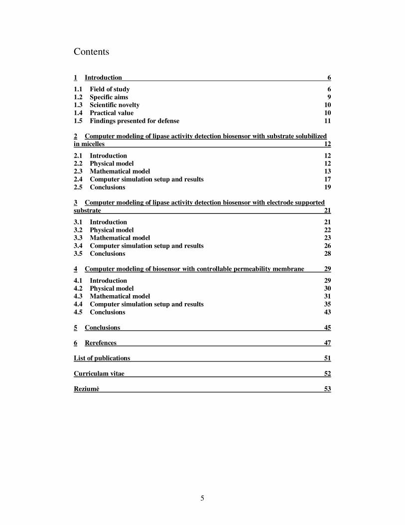
Contents

1 Introduction 6

1.1 Field of study 6 1.2 Specific aims 9 1.3 Scientific novelty 10 1.4 Practical value 10 1.5 Findings presented for defense 11

2 Computer modeling of lipase activity detection biosensor with substrate solubilized

in micelles 12

2.1 Introduction 12 2.2 Physical model 12 2.3 Mathematical model 13 2.4 Computer simulation setup and results 17 2.5 Conclusions 19

3 Computer modeling of lipase activity detection biosensor with electrode supported

substrate 21


4 Computer modeling of biosensor with controllable permeability membrane 29


5 Conclusions 45

6 Rerefences 47

List of publications 51

Curriculam vitae 52

Rezium÷ 53

6

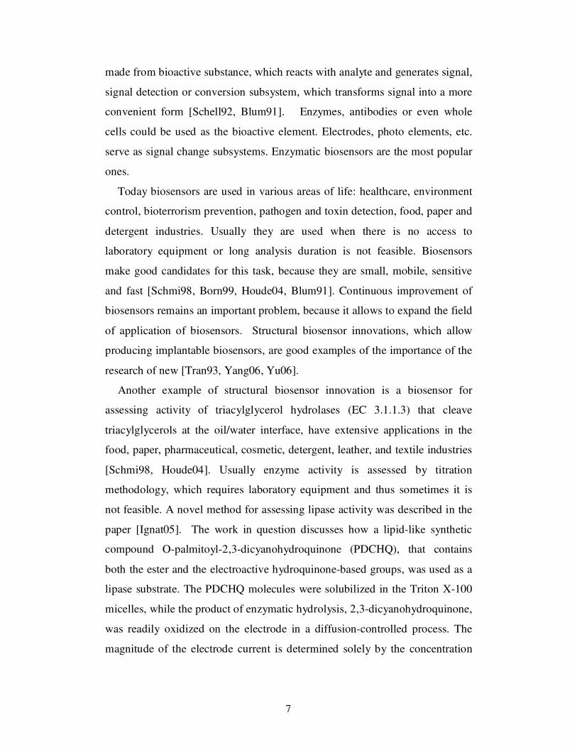
1 Introduction

Computer modeling is a very important method of scientific research. This

method plays an important role in the fields where several different disciplines

of science meet together. Multidisciplinary fields are the most suitable place to

reveal the best features of computer modeling. These best features include

saving human and physical resources, quantum improvement of system

knowledge, also discovery of new knowledge that sometimes cannot be

acquired by direct physical experiments. Biosensors are such multidisciplinary

field where computer modeling can speed up the research. Biosensors are

small analytical devices widely used for environment analysis and control of

complex biotechnological processes or even bioterrorism prevention.

Continuous extension of the field of their application and improvement of

existing biosensors allow to improve the quantity and quality of industrial

products, health care and security. As mentioned above, this is the field where

multiple disciplines are meeting together: physics, chemistry, mathematics and

informatics. Processes happening inside the biosensor, like electrical current

and diffusion, belong to the field of physics. Other processes, like enzyme

binding to the substrate and turning it into product, belong to field of

biochemistry. Mathematics is used to describe these processes in a language of

equations that describe the quantities and relationships among the reacting

components. Only simple cases of these equations could be solved analytically,

so these more complex cases need to be solved using numeric methods on

computers, in other words, computer modeling is performed. Close

collaboration of these sciences is a key to successful improvement of

biosensors.

1.1 Field of study

Biosensors are one of the rapidly changing fields of research and

application. As already mentioned above, biosensors are analytical devices

7

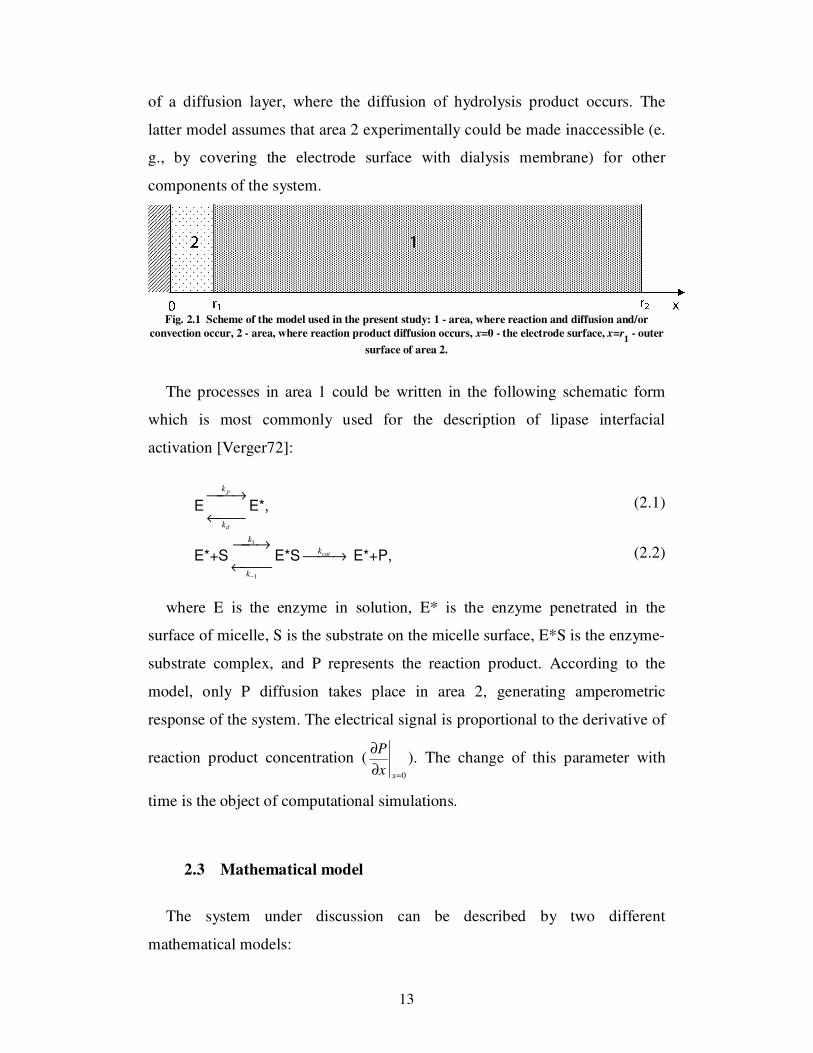
made from bioactive substance, which reacts with analyte and generates signal,

signal detection or conversion subsystem, which transforms signal into a more

convenient form [Schell92, Blum91]. Enzymes, antibodies or even whole

cells could be used as the bioactive element. Electrodes, photo elements, etc.

serve as signal change subsystems. Enzymatic biosensors are the most popular

ones.

Today biosensors are used in various areas of life: healthcare, environment

control, bioterrorism prevention, pathogen and toxin detection, food, paper and

detergent industries. Usually they are used when there is no access to

laboratory equipment or long analysis duration is not feasible. Biosensors

make good candidates for this task, because they are small, mobile, sensitive

and fast [Schmi98, Born99, Houde04, Blum91]. Continuous improvement of

biosensors remains an important problem, because it allows to expand the field

of application of biosensors. Structural biosensor innovations, which allow

producing implantable biosensors, are good examples of the importance of the

research of new [Tran93, Yang06, Yu06].

Another example of structural biosensor innovation is a biosensor for

assessing activity of triacylglycerol hydrolases (EC 3.1.1.3) that cleave

triacylglycerols at the oil/water interface, have extensive applications in the

food, paper, pharmaceutical, cosmetic, detergent, leather, and textile industries

[Schmi98, Houde04]. Usually enzyme activity is assessed by titration

methodology, which requires laboratory equipment and thus sometimes it is

not feasible. A novel method for assessing lipase activity was described in the

paper [Ignat05]. The work in question discusses how a lipid-like synthetic

compound O-palmitoyl-2,3-dicyanohydroquinone (PDCHQ), that contains

both the ester and the electroactive hydroquinone-based groups, was used as a

lipase substrate. The PDCHQ molecules were solubilized in the Triton X-100

micelles, while the product of enzymatic hydrolysis, 2,3-dicyanohydroquinone,

was readily oxidized on the electrode in a diffusion-controlled process. The

magnitude of the electrode current is determined solely by the concentration

8

and diffusion coefficient of the electroactive species, thus proportional to the

activity of the enzyme [Ignat05, Bard01].

Another novel electrochemical technique for the assay of lipase activity has

been described by [Valin05]. The method utilizes a solid supported lipase

substrate, which is formed by dripping and drying a small amount of an

ethanol solution of 9-(5’-ferrocenylpentanoyloxy)nonyl disulfide (FPONDS;

[Fc-(CH2)4COO(CH2)9S-]2, where Fc is the ferrocene) on the gold electrode

surface modified by a hexanethiol self-assembled monolayer. The redox-active

ferrocene group of FPONDS generates the amperometric signal, the intensity

of which is proportional to the number of FPONDS molecules at the interface.

Electrochemical signal decay rate is proportional to the enzyme activity.

Biosensors described above are distinguishable from other biosensors by use

of substrate as bioactive component instead of enzyme. This is a structural

innovation. Controllable permeability membrane could be seen as another

structural biosensor innovation. Theoretical premises for such biosensor do

exist, i.e. there are substances that change their permeability depending on

received charge or medium pH [Shimi88]. Such theoretical premises still need

to be verified. One of ways to perform such analysis is the application of

mathematical and computer modeling.

Computer modeling is one of most important tools used to continuously

create new and improve the already existing biosensors. The main goal of

computer modeling is to identify which factors (e.g. chemical reaction rate,

diffusion rate, activity of the bioactive element) are the most important for the

biosensor’s response to the concentration of analyte. A mathematical model

describes physical and chemical processes that happen inside of the biosensor.

Computer simulation performed according to this model allows to observe and

interact with these processes at a desired scale. Usually several processes are

happening inside a biosensor simultaneously, like the interaction of the enzyme

and the substrate, dissipation of the formed complex, the oxidation/reduction

of the reaction product on the electrode, diffusion of all acting substances.

Relative importance of each of these processes cannot be evaluated with single

9

experiment [Coop04]. Series of such experiments with variable parameters in

comparison to the kinetic model allows to obtain more extensive knowledge of

the system in question. Mathematical model and computer simulation are the

instruments that allow to plan the future experiments and improve biosensor

parameters so that they are better fitted specific application. If there were no

mathematical model, the researchers should perform massive amount of

physical experiments and go through trials and errors to achieve the same

amount of knowledge about how the system works [Coop04]. Computer

modeling saves time and resources required for physical experiments and

allows to expand the knowledge on how the system works, which is a key to

successful improvement of biosensors.

1.2 Specific aims

• Select and apply mathematical and computer models for a lipase

activity assessing biosensor with the substrate solubilized in micelles.

Verify applicability of the selected model. Analyze what would be

the biosensor response time if the sensor works under the selected

model.

• Select and apply mathematical and computer models for lipase

activity assessing biosensor with the electrode supported substrate.

Verify applicability of the selected model. Analyze what would be

specific biosensor features and parameters if it works under the

selected model.

• Perform computer modeling and analyze the effect of replacing the

static membrane with a controllable permeability membrane on

biosensor response.

10

1.3 Scientific novelty

The computer simulation was applied to evaluate the enzymatic reaction rate

constant for lipase (Thermomyces lanuginosus) activity assessing biosensor

with substrate (O-palmitoyl-2,3-dicyanohydroquinone) solubilized in micelles

basing on computer simulation results. It turned out that the constant substrate

concentration cannot be assumed, and the kinetic equation system described in

[Verger72] should be extended by adding the substrate kinetic equation.

The proposed original kinetic model extension with non-linear second order

term for lipase activity assessment biosensor with the electrode supported

substrate yielded better results than the classical one. By analyzing the results

of the physical experiment it was discovered that the substrate concentration on

the electrode decay is expressed in two types of dependencies on time, the

exponential one, and the one proportional to t-1.

A mathematical model for original biosensor with controllable permeability

membrane was proposed. The proposed original model takes into account

medium pH and temperature. It was discovered that using a membrane the

permeability of which nonlinearly changes depending on the medium pH, the

biosensor could easily be switched from kinetic to diffusion mode, and the

linear response range could be extended by several magnitudes. It was shown

that a membrane the permeability of which is controllable in time could be

superior to the static membrane when the biosensor operates in the

electrochemical stripping mode, and the reaction product inhibition to the

enzymatic reaction is low.

1.4 Practical value

Presented findings on the specific features of the two novel lipase activity

assessing biosensors make ground for the evaluation of the feasibility of the

production of such sensors . A detailed analysis of the innovative biosensor

11

with controllable permeability membrane shows that production of such

biosensors might be feasible in some specific cases.

1.5 Findings presented for defense

1. The constant substrate concentration on the micelle surface cannot be

assumed for the lipase activity assessing biosensor with the substrate

solubilized in micelles. The kinetic model originally described by

[Verger72] and extended with the substrate kinetic equation allows

for a good fit of physical experiment and computer simulation results

when it is assumed that the biosensor is a closed system.

2. The proposed original kinetic model extension with the second order

nonlinear substrate wash off term for the lipase activity assessing

biosensor with the electrode supported substrate yields better fitting

with physical experiment data than the classic reaction model.

3. By replacing the biosensor's static membrane with a membrane the

permeability of which nonlinearly depends on medium pH, it is

possible to produce a biosensor that would be easily reconfigurable

(by switching between kinetic and diffusion modes) between very

sensitive and wide linear response range modes.

4. The biosensor with a membrane that controllably changes its

permeability in time would be superior to a biosensor with a static

membrane, assuming that the biosensor operates in an

electrochemical stripping mode and the enzymatic reaction inhibition

by the reaction product is low.

12

2 Computer modeling of lipase activity detection

biosensor with substrate solubilized in micelles

2.1 Introduction

Recently, the amperometric detection method of Thermomyces lanuginosus

lipase activity has been published [Ignat05]. Lipases, triacylglycerol

hydrolases (EC 3.1.1.3) that cleave triacylglycerols at the oil/water interface,

have extensive applications in the food, paper, pharmaceutical, cosmetic,

detergent, leather, and textile industries [Schmi98, Houde04]. Widespread

practical use of these enzymes requires fast and reliable analytical routines to

assess their activity. The electrochemical technique, described in [Ignat05],

presents the method of this kind.

In the work under discussion, a lipid-like synthetic compound O-palmitoyl-

2,3-dicyanohydroquinone (PDCHQ), that contains both the ester and the

electroactive hydroquinone-based groups, was used as a lipase substrate. The

PDCHQ molecules were solubilized in the Triton X-100 micelles, while the

product of enzymatic hydrolysis, 2,3-dicyanohydroquinone, was readily

oxidized on the electrode in a diffusion-controlled process. Under the diffusion

control, the magnitude of the electrode current is determined solely by the

concentration and diffusion coefficient of the electroactive species (in the case

of work [Ignat05], 2,3-dicyanohydroquinone) and the effective thickness of the

diffusion layer [Bard01].

The authors of the paper [Ignat05] have performed experiments under the

steady-state conditions. The aim of the present work is computational

modeling of response kinetics of this bioelectroanalytical system.

2.2 Physical model

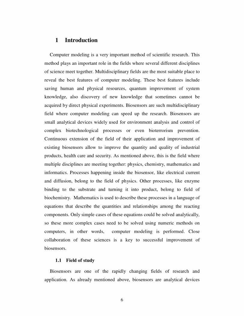
In a simplified one-dimension model (Fig. 2.), the working space of

bioelectroanalytical system described in [Ignat05] could be divided into two

parts: the first one - wide area, where enzymatic reaction and

molecular/particle (convective-)diffusion occur, the second one - narrow area

13

of a diffusion layer, where the diffusion of hydrolysis product occurs. The

latter model assumes that area 2 experimentally could be made inaccessible (e.

g., by covering the electrode surface with dialysis membrane) for other

components of the system.

Fig. 2.1 Scheme of the model used in the present study: 1 - area, where reaction and diffusion and/or

convection occur, 2 - area, where reaction product diffusion occurs, x=0 - the electrode surface, x=r1 - outer

surface of area 2.

The processes in area 1 could be written in the following schematic form

which is most commonly used for the description of lipase interfacial

activation [Verger72]:

E←

→

d

p

k

k

E*, (2.1)

E*+S

←

→

−1

1

k

k

E*S → catk E*+P, (2.2)

where E is the enzyme in solution, E* is the enzyme penetrated in the

surface of micelle, S is the substrate on the micelle surface, E*S is the enzyme-

substrate complex, and P represents the reaction product. According to the

model, only P diffusion takes place in area 2, generating amperometric

response of the system. The electrical signal is proportional to the derivative of

reaction product concentration (0=∂

∂

xx

P). The change of this parameter with

time is the object of computational simulations.

2.3 Mathematical model

The system under discussion can be described by two different

mathematical models:

14

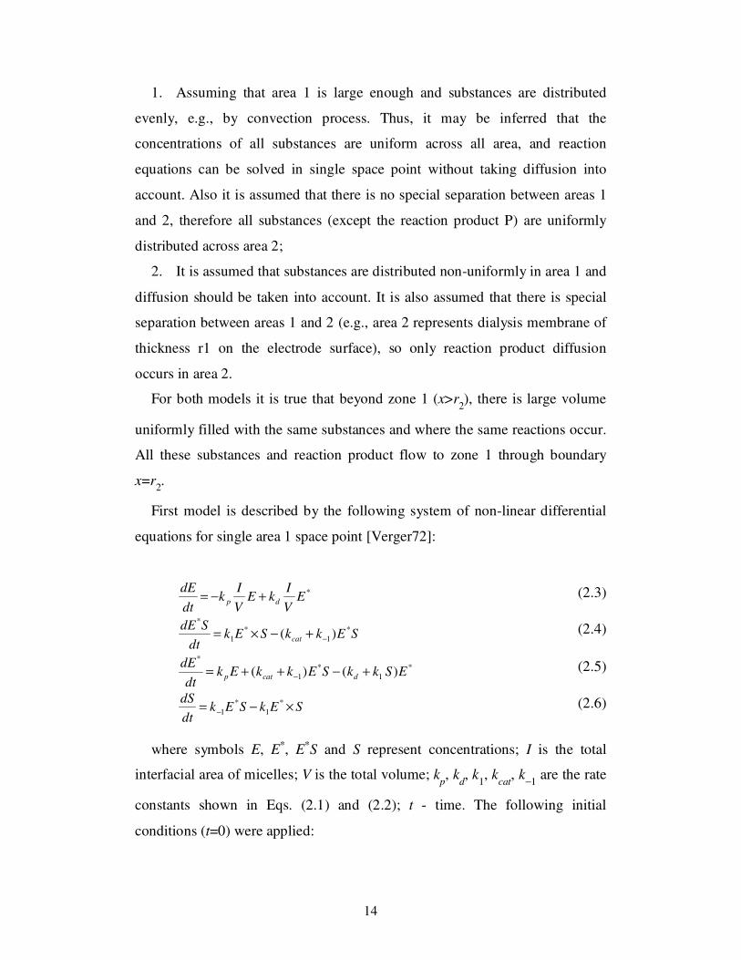
1. Assuming that area 1 is large enough and substances are distributed

evenly, e.g., by convection process. Thus, it may be inferred that the

concentrations of all substances are uniform across all area, and reaction

equations can be solved in single space point without taking diffusion into

account. Also it is assumed that there is no special separation between areas 1

and 2, therefore all substances (except the reaction product P) are uniformly

distributed across area 2;

2. It is assumed that substances are distributed non-uniformly in area 1 and

diffusion should be taken into account. It is also assumed that there is special

separation between areas 1 and 2 (e.g., area 2 represents dialysis membrane of

thickness r1 on the electrode surface), so only reaction product diffusion

occurs in area 2.

For both models it is true that beyond zone 1 (x>r2), there is large volume

uniformly filled with the same substances and where the same reactions occur.

All these substances and reaction product flow to zone 1 through boundary

x=r2.

First model is described by the following system of non-linear differential

equations for single area 1 space point [Verger72]:

*EV

IkE

V

Ik

dt

dEdp +−= (2.3)

SEkkSEk

dt

SdEcat

*1

*1

*

)( −+−×= (2.4)

*

1*

1

*

)()( ESkkSEkkEkdt

dEdcatp +−++= − (2.5)

SEkSEk

dt

dS×−= −

*1

*1 (2.6)

where symbols E, E*, E*S and S represent concentrations; I is the total

interfacial area of micelles; V is the total volume; kp, k

d, k

1, k

cat, k

−1 are the rate

constants shown in Eqs. (2.1) and (2.2); t - time. The following initial

conditions (t=0) were applied:

15

E(0) = E0,

E*(0) = 0, E

*S(0) = 0,

S(0) = S0

(2.7)

Additional equation for area 2 (product diffusion plus gain from reactions in

this area):

),0(, 1*

2

2

rxSEV

Ik

x

PD

t

Pcatp ∈+

∂

∂=

∂

∂, (2.8)

where symbol P represents reaction product concentration; d

p is the

diffusion coefficient of P; x - distance, E*S is calculated from solution of

equation system (2.3)-(2.6) . Initial condition (t=0) for the second part of

calculations:

P(0,x) = 0, x ∈ [0,r1], (2.9)

whereas boundary conditions:

P(t,0) = 0, t > 0 (2.10)

and

∂P

∂t= kcat

I

VE

*S, x = r1, t > 0, (2.11)

which is calculated from solution of equation system (2.3)-(2.6).

The second model is described by the system of non-linear partial differential equations [Verger72]:

2

2*

x

EDE

V

IkE

V

Ik

t

EEdp

∂

∂++−=

∂

∂

(2.12)

2

*2*

1*

1

*

*)(x

SEDSEkkSEk

t

SESEcat

∂

∂++−×=

∂

∂−

(2.13)

2

*2

1*

1

*

*)()(x

EDSkkSEkkEk

t

EEdcatp

∂

∂++−++=

∂

∂− (2.14)

2

2*

1*

1x

SDSEkSEk

t

SS

∂

∂+×−=

∂

∂− (2.15)

16

for area x ∈ (r1 , r2 ). Definitions are the same as for the first model, and dE,

dE

*S, d

E*, d

S are the diffusion coefficients of free enzyme, micellar enzyme-

substrate complex, micelle with penetrated enzyme (in fact, dE

*S=d

E*), and

substrate, respectively. Reaction product generation and diffusion equation is

as follows:

),0(, 2*

2

2

rxSEV

Iqk

x

PD

t

PcatP ∈+

∂

∂=

∂

∂,

∈

∈=

.),(,1

];,0(,0

21

1

rrx

rxq

(2.16)

Initial conditions (t=0):

E*(0, x) = 0,E *

S(0,x) = 0,

E(0,x) = E0,S(0, x) = S0, x ∈ [r1,r2];

P(0,x) = 0, x ∈ [0,r2].

(2.17)

Boundary conditions:

P(t,0) = 0, t > 0; (2.18)

no flow condition for subregions boundary point x = r1, t > 0:

0)(,0)(,0)(,0)(

1111

**

=∂

∂=

∂

∂=

∂

∂=

∂

∂

====

tx

Et

x

SEt

x

St

x

E

rxrxrxrx

(2.19)

and boundary condition for point x = r2 , t > 0:

).()(

),()(),()(

),()(),(Pr)(

2**

2**

2

22

2

22

22

trEtE

tSrEtSEtSrtS

tErtEttP

rx

rxrx

rxrx

=

==

==

=

==

==

(2.20)

Pr2 , Er2 , E*r2 , E*Sr2 are calculated from solution of equation system (2.3)-

(2.6).

17

2.4 Computer simulation setup and results

Dedicated software package was developed to automate computer modeling

of the system under study. Matlab was chosen as environment for such

software package development. Using this software package the series of

computational simulations were performed to investigate how electrode

readings would differ if bioelectroanalytical system worked under the first or

second model.

The first simulation experiment was designed according to the first model of

bioelectroanalytical system. Calculations were divided into two steps: in the

first step, calculations were performed according to Eqs. (2.3)-(2.6), and in

second step, the diffusion of P was calculated for area 2 according to Eq. (2.8).

The following values were used in calculations (all parameters, except kinetic

constants, are from [Ignat05]): DP = 5.49·10−5 cm2 s−1 , r1 = 4·10−3 cm, I =

7.5·105 cm2 , V = 10 cm3 , E0 = 2.35·10−8 mol cm−3 , kcat = 75 s−1 , k1 = 1.12·109

cm2 mol−1 s−1 , k−1 = 10 s−1 , kp = 100 cm s−1 , kd = 0.025 s−1 , S0 = 6.7·10−12

mol cm−2. First step calculations were performed using Matlab ODE solver for

stiff problems. For the second part of calculations the system of differential

equations was discretized using the implicit finite difference scheme

[Samar01], system of linear equations corresponding to this scheme was solved

using matrix solver for tridiagonal matrices. Integration steps in space and time

were as follows: hx=5⋅10−6cm, h

t=1s; integration in time interval was

T=[0..3000]. The results of computational experiment are presented in Fig. 2.2.

18

Fig. 2.2 △△△△ – recalculated experimental data points from [Ignat05] (

0=∂

∂

xx

P (in mol cm−4 ) dependency on

time); solid line - computed

0=∂

∂

xx

P (in mol cm−4 ) dependency on time (in seconds) according to the first

model of bioelectroanalytical system.

Fig. 2.2 also contains the recalculated data points from ref. [Ignat05]. For

the rotating disk electrode employed in [Ignat05], 0=∂

∂

xx

P= I/(nFAdP) [Bard01],

where I is the experimental current values, n=2 is the number of electrons

transferred during the oxidation of P, F is the Faraday constant, and

A=0.07 cm2 is the electrode surface area. As can be seen from Fig. 2.2, the

mathematical model (model 1) and a set of kinetic constants used in the

computational experiment enabled to attain good agreement between the

experimental and modeling results. It is believed that systematically slightly

higher values of experimental data points in Fig. 2.2 result from imperfect

subtraction of background current in work [Ignat05]. Unfortunately, because of

complexity of interfacial lipase action (see Eqs. (2.1) and (2.2)), individual

kinetic constants for this enzyme are not reported in the literature. This fact

presents difficulties to check the validity of the kinetic constants used in

calculations.

The second experiment was designed according to the second model of

amperometric system. Constant values were the same as for the first

experiment, additionally the second stagnant diffusion layer was defined:

cmr 32 108 −×= ; d

E*S=10−7 cm2 s−1, d

E*=10−7 cm2 s−1, d

E=10−6 cm2 s−1,

19

dS=10−6 cm2 s−1, when r

1≤x≤r

2 and, for the diffusion coefficients, zero in other

cases. Differential equation system was transformed into implicit finite

differences scheme and non-linear equation system corresponding to this

scheme was solved using simple iterations method [Samar01]. The results are

presented in Fig. 2.3 (continuous line). The same experiment was repeated two

more times with following boundary location pairs a) r1=8 10−4, r2=4.8 10−3; b)

r1=4 10−4, r2=4.4 10−3 (all values in cm).

Fig. 2.3 Solid line -

0=∂

∂

xx

P (in mol cm−4 ) dependency on time (in seconds) according to the second model

of analytical system and assuming r1=4⋅⋅⋅⋅10−−−−3 cm and r

2=8⋅⋅⋅⋅10−−−−3 cm; dashed line - r

1=8⋅⋅⋅⋅10−−−−4 cm and

r2=4.8⋅⋅⋅⋅10−−−−3 cm; and dotted line - r

1=4⋅⋅⋅⋅10−−−−4 cm and r

2=4.4⋅⋅⋅⋅10−−−−3 cm.

2.5 Conclusions

The results of foregoing computational experiments enable to make the

following conclusions:

1. Model described by [Verger72] cannot be applied directly for

Thermomyces lanuginosus lipase activity assessing biosensor. Constant

substrate concentration cannot be assumed thus model should be extended with

substrate kinetic equation. Such model extension allows obtaining good fit

between experimental and computer simulation results.

2. An enzymatic reaction rate constant for Thermomyces lanuginosus

lipase with respect to the synthetic substrate, O-palmitoyl-2,3-

dicyanohydroquinone, is suggested (in context of set of other individual kinetic

constants) in the computational experiments.

20

3. As expected, modeling of the analytical system with additional stagnant

diffusion layer (the diffusion layer in model 1 is replaced by the dialysis

membrane of the same thickness, and the second diffusion layer of constant

thickness in model 2 is formed, for instance, by electrode rotation)

demonstrates a decreased initial rate of system response (i.e., rate of current

increase upon enzyme injection in the system). Computational experiments

also show that significant decrease of dialysis membrane thickness and

increase of electrode rotation rate (leads to the decreased thickness of the

second diffusion layer) should improve the performance of the analytical

system. Electrochemical experiments along these lines are in progress.

21

3 Computer modeling of lipase activity detection

biosensor with electrode supported substrate

3.1 Introduction

Lipolytic enzymes are one of the most important components of the

biochemical processes. At the same time, triacylglycerol acylhydrolases (EC

3.1.1.3) that hydrolyze triacylglycerols at the oil/water interface have wide

applications as detergent additives, digestive aids, as well as in the paper and

food industries [Schmi98, Born99, Houde04]. Unlike other bond-cleaving

enzymes, e.g., proteases, hydrolysis by lipases is carried out in heterogeneous

multiphase systems. In many cases, the environment of the enzyme at the

substrate/liquid interface plays an important role for the overall enzymatic

activity of these proteins [Schmi98, Born99, Houde04, Beiss00]. Thus, the

ability to monitor enzymatic activity of lipases under these conditions is of

paramount importance.

Recently, a novel electrochemical technique for the assay of lipase activity

has been described [Valin05]. The method utilizes a solid supported lipase

substrate, which is formed by dripping and drying a small amount of an

ethanol solution of 9-(5’-ferrocenylpentanoyloxy)nonyl disulfide (FPONDS;

[Fc-(CH2)4COO(CH2)9S-]2, where Fc is the ferrocene) on the gold electrode

surface modified by a hexanethiol self-assembled monolayer. The redox-active

ferrocene group of FPONDS generates the amperometric signal, the intensity

of which is proportional to the number of FPONDS molecules at the interface.

Electrochemical and surface-enhanced infrared absorption spectroscopic data,

as well as control experiments with an engineered, deactivated mutant enzyme,

have demonstrated that the wild-type lipase from Thermomyces lanuginosus

(TLL) is capable of cleaving the ester bonds of FPONDS molecules via an

enzymatic hydrolysis mechanism, which includes the adsorption of the lipase

onto the substrate surface. The interfacial enzymatic process liberates

ferrocene groups from the electrode surface triggering a decay of the

22

electrochemical signal. The rate of the electrochemical signal decrease is

proportional to the lipase activity.

However, in exclusively experimental work [Valin05], no kinetic model has

been proposed to account for the features of amperometric biosensor response,

namely, current decay vs. time upon enzyme action. This paper is intended to

fill this gap.

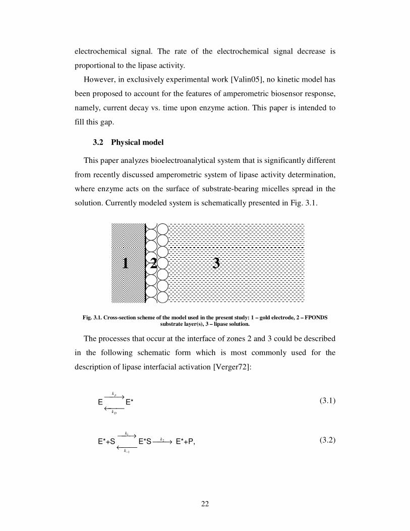
3.2 Physical model

This paper analyzes bioelectroanalytical system that is significantly different

from recently discussed amperometric system of lipase activity determination,

where enzyme acts on the surface of substrate-bearing micelles spread in the

solution. Currently modeled system is schematically presented in Fig. 3.1.

Fig. 3.1. Cross-section scheme of the model used in the present study: 1 – gold electrode, 2 – FPONDS

substrate layer(s), 3 – lipase solution.

The processes that occur at the interface of zones 2 and 3 could be described

in the following schematic form which is most commonly used for the

description of lipase interfacial activation [Verger72]:

E

←

→

D

p

k

k

E* (3.1)

E*+S

←

→

−1

1

k

k

E*S → 2k E*+P, (3.2)

1 2 3

23

where E is the enzyme in solution, E* is the enzyme attached to the surface

of substrate (at the interface of zones 2 and 3 in Fig. 3.1), S is the ferrocene-

based substrate FPONDS substrate on the gold electrode surface, E*S is the

enzyme-substrate complex, and P represents the reaction product. The change

of S concentration as a function time is the object of computational simulations

as it is directly proportional to experimentally registered electrode signal (see,

for instance, Fig. 1 in [Valin05]).

3.3 Mathematical model

It is assumed that lipase solution is distributed evenly and its diffusion could

be not taken into account. It is also assumed that the redox-active reaction

product (ferrocene-based) leaves sensor surface quite fast and its diffusion

could be estimated as instantaneous. The system under discussion can be

described by classical mathematical model of reaction kinetics:

−

=

=

×−=

−−×=

−+×−+=

−

−

−

EkV

IEk

V

I

dt

dE

SEkdt

dP

SEkSEkdt

dS

SEkSEkSEkdt

SdE

EkEkSEkSEkSEkdt

dE

pD

Dp

*

*2

*1

*1

*2

*1

*1

*

**1

*2

*1

*

(3.3)

where symbols in italics E, E*, E*S, P and S represent concentrations; I is

the interfacial area of electrode; V is the total volume of solution; kp is the rate

constant of enzyme adsorption at the electrode surface, kD is the enzyme

desorption rate constant, k1 is the rate constant of enzyme-substrate complex

(E*S) formation, k-1 is the rate constant of E*S dissociation, k2 is the catalytic

rate constant of enzymatic reaction, and t is time.

This model allowed good fitting only for a part of experimental data

available (data not shown), which had strongly expressed exponential character

24

of substrate concentration decrease (Fig. 3.2, experiment B; for the

characteristics of different experiments, see parameters in the table).

Fig. 3.2. Experiment A and B data analysis: ▲- 1/S dependency on time;▼- ln(S) dependency on time.

However, another part of experimental data exhibited S decrease

asymptotically proportional to t-1 (Fig. 3.2, experiment A). Thus, the model of

Eq. (3.3) was modified by adding a non-linear term of substrate wash off from

the electrode surface, which allowed much better fitting results. Here, it should

be noted that in work [Valin05] the wash off effect of substrate has been

observed experimentally in the solutions without added enzyme (see Fig. 1 in

paper [Valin05]). Therefore, we have reasonable grounds to believe that this

process also occurs in the solutions containing enzyme.

0 1000 2000 3000 4000 5000 6000 0

0.5

1

1.5

2

2.5

3

3.5

4

x 10 -11

t,s

S,

mol c

m

-2

Experiment D

0 1000 2000 3000 4000 5000 60000

0.5

1

1.5

2

2.5

3

3.5

x 10 -10

t,s

S,

mol cm

-2

Experiment A

0 1000 2000 3000 4000 5000 60000

1

2

3

4

5

6

7

8

9x 10

-10

t,s

S,

mol cm

-2

Experiment B

0 1000 2000 3000 4000 5000 0

0.5

1

1.5

2

2.5

3

3.5

x 10 -10

t,s

S,

mol c

m

-2

Experiment C

6000

25

Thus, slightly modified system of non-linear differential equations can be

written by Eq. (3.4):

−

=

=

−×−=

−−×=

−+×−+=

−

−

−

EkV

IEk

V

I

dt

dE

SEkdt

dP

S

SkSEkSEk

dt

dS

SEkSEkSEkdt

SdE

EkEkSEkSEkSEkdt

dE

pD

S

Dp

*

*2

2

0

*1

*1

*2

*1

*1

*

**1

*2

*1

*

(3.4)

where definitions are the same as for Eq. (3.3), and kS is the substrate wash

off rate constant and S0 is the initial substrate concentration on the electrode

surface.

Non-linear wash off term is quite unusual, but it could be explained in a

simplified way as complex outcome of two different linear wash off rates: one

for the electrode surface/substrate boundary (stronger bond, lower wash off

rate) and second (weaker attraction, much higher wash off rate) for, say,

substrate/substrate boundary. It is possible that during the process of modified

electrode preparation substrate forms only very few substrate/substrate

boundaries (pseudo-multilayer interfacial structure). Thus, initially wash off

rate could be seen as linearly (in respect to the substrate concentration)

dropping from high value for the substrate/substrate boundary, down to low

value for the electrode/ substrate boundary, and the whole process then

becomes second order with respect to the substrate concentration. By way of

illustration, let’s assume that the wash-off rate constant (k) changes linearly

with relative substrate concentration: k=a·S/S0+b, where a and b are the

constants, so non-linearity could be introduced by substituting the wash-off

rate constant in standard linear wash-off model: dS/dt = -kS.

26


Software package described in a chapter above was extended to support

extended variety of models, like models assuming additional intermeadiate

state in enzymatic reaction or models assuming nonlinear substrate wash off

terms. The series of computational simulations were performed using this

software package to investigate how electrode readings would differ if this

amperometric biosensor worked under presented model and how they would

match experimental data (experimental results were obtained as described in

[Valin05], converting the integrated electrode peak current of the FPONDS-

modified electrode to the surfaces concentration of ferrocene functional

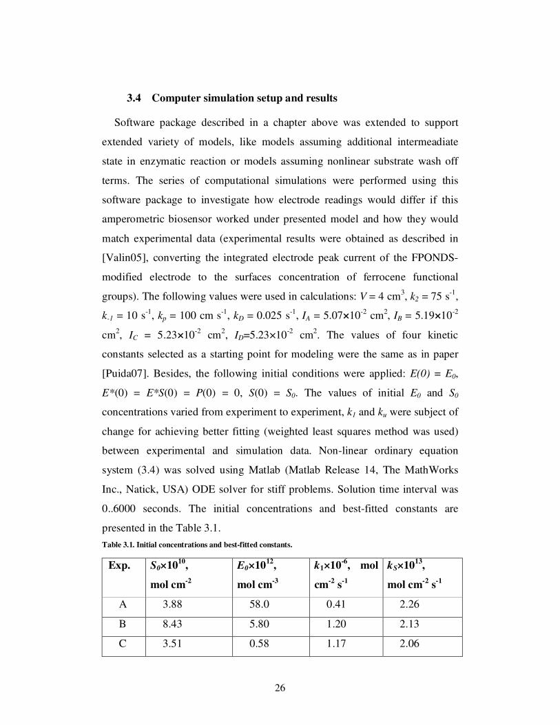
groups). The following values were used in calculations: V = 4 cm3, k2 = 75 s-1,

k-1 = 10 s-1, kp = 100 cm s-1, kD = 0.025 s-1, IA = 5.07×10-2 cm2, IB = 5.19×10-2

cm2, IC = 5.23×10-2 cm2, ID=5.23×10-2 cm2. The values of four kinetic

constants selected as a starting point for modeling were the same as in paper

[Puida07]. Besides, the following initial conditions were applied: E(0) = E0,

E*(0) = E*S(0) = P(0) = 0, S(0) = S0. The values of initial E0 and S0

concentrations varied from experiment to experiment, k1 and ku were subject of

change for achieving better fitting (weighted least squares method was used)

between experimental and simulation data. Non-linear ordinary equation

system (3.4) was solved using Matlab (Matlab Release 14, The MathWorks

Inc., Natick, USA) ODE solver for stiff problems. Solution time interval was

0..6000 seconds. The initial concentrations and best-fitted constants are

presented in the Table 3.1.

Table 3.1. Initial concentrations and best-fitted constants.

Exp. S0×1010

,

mol cm-2

E0×1012

,

mol cm-3

k1×10-6

, mol

cm-2

s-1

kS×1013

,

mol cm-2

s-1

A 3.88 58.0 0.41 2.26

B 8.43 5.80 1.20 2.13

C 3.51 0.58 1.17 2.06

27

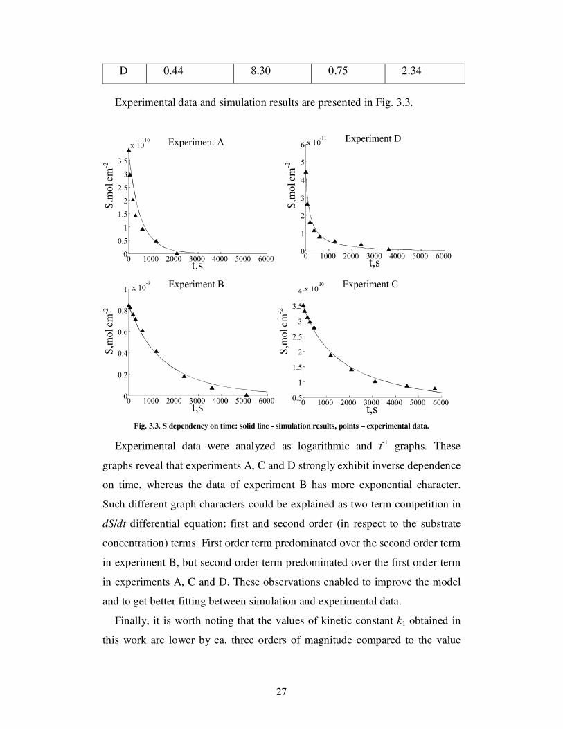
D 0.44 8.30 0.75 2.34

Experimental data and simulation results are presented in Fig. 3.3.

Fig. 3.3. S dependency on time: solid line - simulation results, points – experimental data.

Experimental data were analyzed as logarithmic and t-1 graphs. These

graphs reveal that experiments A, C and D strongly exhibit inverse dependence

on time, whereas the data of experiment B has more exponential character.

Such different graph characters could be explained as two term competition in

dS/dt differential equation: first and second order (in respect to the substrate

concentration) terms. First order term predominated over the second order term

in experiment B, but second order term predominated over the first order term

in experiments A, C and D. These observations enabled to improve the model

and to get better fitting between simulation and experimental data.

Finally, it is worth noting that the values of kinetic constant k1 obtained in

this work are lower by ca. three orders of magnitude compared to the value

S,m

ol cm

-2

S,m

ol cm

-2S

,mol

cm-2

S,m

ol cm

-2

28

reported in a study [Puida07]. Most likely, the difference is determined by

different chemical nature of substrate head-groups in work [Puida07]

(dicyanohydroquinone-based group) and the present study (ferrocene-based

group), since k1 reflects molecular event of substrate binding in the enzyme

active center.

3.5 Conclusions

The results of the foregoing computational experiments enable to make the

following conclusions:

1. The proposed reaction kinetic model of response of the FPONDS-based electrode, used for the electrochemical determination of Thermomyces

lanuginosus lipase activity, allows achieving a good fit between experimental data and simulation results.

2. According to the results of study, experimental data exhibit two distinct types of substrate (FPONDS) concentration decay: one exponential (in respect to time) and the other of t-1-type. This indicates that, in the dU/dt differential equation in system Eq (3.4), first and second order (in respect to the substrate concentration) terms are competing and should be taken into account in numeric modeling.

3. Numeric simulations have revealed that a good fitting might be obtained only taking into account non-linear substrate wash off process, which could be explained in a simplified way as a complex outcome of two different linear wash off rates: one for the electrode surface/substrate boundary (stronger bond, lower wash off rate) and the other (weaker attraction, much higher wash off rate) for the substrate/substrate layer boundary. In this model of interface, it is assumed that substrate forms only very few substrate/substrate boundaries (pseudo-multilayer interfacial structure), thus wash off rate could be seen as linearly (with respect to the substrate concentration) dropping from high value for substrate/substrate boundary, down to low value for electrode surface/substrate boundary, therefore the whole process then becomes second order with respect to the substrate concentration.

29

4 Computer modeling of biosensor with controllable

permeability membrane

4.1 Introduction The action of the biosensor is determined by a number of the parameters

attributed to the: (i) biological system, such as the catalytical capacity of the

biosensor, the rate of the bounding of the substrate, rate of the conversion of

the substrate; (ii) the transducer, such as the rate of the conversion of the

product of the enzymatic reaction, the rate of the regeneration of the

electrochemical system; (iii) diffusion parameters and the rates of the substrate

diffusion into active center, the rate of diffusion of the product to the

electrochemical system, the diffusion of the products of electrochemical

conversion [Turner87]. All these mentioned parameters are constant during the

considerable time of biosensor action. The slowest process is identified as a

rate limiting step and determines the parameters of the biosensor. The

electrochemical reactions are usually very fast compared to the enzymatic

process and diffusion parameters. Thereby, there are two groups of parameters,

responsible for biosensor action: biocatalytic - determined by the parameters of

enzymatic conversion, and diffusion - determined by the construction of the

biosensor. On the basis of these two groups of parameters two limiting

biosensor action modes were identified. The first one – the kinetic mode is

realized when the activity of the enzymatic conversion of the substrate is very

low in comparison with the diffusion parameters. In this case all parameters of

the biosensor are determined by the parameters of the catalytic process. It

means, that the pH dependence of the biosensor response will be the same as

the pH dependence of the enzyme activity, and the temperature dependence of

the response will be determined by activation energy of the catalytic process

(usually about 10 %/deg.) etc. The linearity of the biosensor response (linear

dependence of the biosensor response to the substrate concentration) is usually

30

determined by the value of KM and is very short. The sensitivity of the

response (response to concentration ratio) is quite high.

Another limiting mode – the diffusion mode, is realized when the catalytic

activity of the biosensor is very high and the slowest step is a substrate

diffusion to the active center of enzyme. At this mode the parameters of the

biosensor are determined by the diffusion parameters. If the pH change does

not affect diffusion parameters, it means that biosensor response is insensitive

to the pH fluctuations in the bulk. The influence of the temperature on the

diffusion is much lower (about 2-3 %/deg.). The sensitivity of the biosensor is

low. When the biosensor operates in the diffusion mode, a long linear

calibration curve of the biosensor can be expected. It is a good feature, because

biosensor can operate at high concentrations of the substrate. For example,

linearity of glucose biosensors, designed on glucose oxidase [Laurin89] or

PQQ glucose dehydrogenase [Laurin04] usually reach only few mM. Only in

some cases it can be extended up to 15 mM [Laurin04, Kanap92]. This can be

achieved by switching biosensor action into deep diffusion mode, or artificially

lowering the concentration of the substrate on the outer surface of the outer

membrane. These modes of the biosensor action were described in a (large)

number of papers [Mell75, Kulys86, Schul97, Baron02, Baron03, Baron04].

The possibility of switching the modes of action opens up a nice opportunity

to manage analytical parameters of the biosensor. Sometimes it is useful,

especially, when the biosensor operates in a system where the substrate

concentration varies on large scale.

The goal of this paper is the mathematical modeling of the biosensor action,

where the catalytic capacity of the biosensor is affected by the pH, and when

the diffusion parameters of the membrane can be regulated. The response time

and the linearity of the biosensor will also be analyzed.

4.2 Physical model The flat biosensor with the enzyme layer deposited on the flat electrode and

covered with the flat membrane has been investigated. A number of

31

electrochemical biosensors have such construction. Even if the outer

membrane is omitted, the thickness of enzymatic layer on the surface of the

electrode and non- mixing solvent layers act like the outer membrane. It is

assumed that the thickness of the enzyme layer is c and stable during all

procedure. Flat porous membrane of thickness δ=d-c possess flexible thickness

and permeability characterized by diffusion coefficients for substrate and

reaction product DSM = DPM = Dmembr.. The enzyme activity and the membrane

permeability are dependent on the pH. Currently modeled system is

schematically presented in Fig. 4.1.

Fig. 4.1. Cross-section scheme of the model used in the present study: 1 – electrode, 2 – enzyme layer, 3 – membrane.

4.3 Mathematical model It is assumed the classical scheme, where enzyme (E) converts substrate (S)

into reaction product (P):

PS E→ (4.1)

Such a biosensor mathematical model could be described by using two

dimensional reaction−diffusion equations containing a nonlinear term related

to the Michaelis−Menten kinetics with the reaction product inhibition. In this

case, it is additionally assumed that the diffusion coefficients and the enzyme

3 2

0 c d x

1

32

activity are dependent on the pH and the temperature. Equations governing the

processes occurring in area 2 (Fig. 4.1) are [Frey07]:

++⋅

⋅+

∂

∂=

∂

∂

++⋅

⋅−

∂

∂=

∂

∂

SKPK

STpHV

x

PTD

t

P

SKPK

STpHV

x

STD

t

S

PM

Max

PE

PM

Max

SE

)/1(

),()(

)/1(

),()(

2

2

2

2

, ),0( cx ∈ , (4.2)

Equations describing the processes occurring in area 3 are:

∂

∂=

∂

∂∂

∂=

∂

∂

2

2

2

2

),(

),(

x

PTpHD

t

Px

STpHD

t

S

PM

SM

, ),( dcx ∈ , (4.3)

where symbols in italics are S – substrate concentration, DSE, DPE – substrate

and reaction product diffusion coefficients inside area 2, DSM, DPM – substrate

and reaction product diffusion coefficients inside membrane (area 3), VMax –

maximum enzymatic rate, Km – Michaelis constant, KP – reaction product

inhibition constant, T – temperature, pH – pH inside membrane.

The maximum enzymatic rate dependence on the pH is modeled using the

Gauss function with the center pHV=6 and the dependency on temperature is

modeled by the linear function with 10%/degree rate and the center at 20°C:

2)6(0 10

10),( −−⋅

−⋅= pH

MaxMax eT

VTpHV (4.4)

where VMax0 – a typical maximum enzymatic rate at 20°C and the pH = 6.

The diffusion coefficients inside the enzymatic layer (area 2) are modeled

using the linear function with 3%/degree rate and the center at 20°C:

+⋅=

+⋅=

33

13)(

33

13)(

0

0

TDpHD

TDpHD

PEPE

SESE

(4.5)

where DSE0 and DPE0 – the substrate and the reaction product diffusion

coefficient inside the enzymatic layer (area 2) at 20°C temperature. The

33

diffusion coefficients dependency on time inside membranes modeled using

several different models – Gaussian, linear and constant:

⋅=

⋅=−−

−−

2

2

)(

)(

)(),(

)(),(M

M

pHpH

PEPM

pHpH

SESM

eTDTpHD

eTDTpHD, (4.6)

or

−⋅⋅=

−⋅⋅=

)7.02.0()(),(

)7.02.0()(),(

pHTDTpHD

pHTDTpHD

PEPM

SESM , (4.7)

or

⋅=

⋅=

2.0)(),(

2.0)(),(

TDTpHD

TDTpHD

PEPM

SESM . (4.8)

Initial conditions:

S(0,x) = 0, kai x<d; S(0,d) = S0; P(0,x) = 0. (4.9)

Boundary conditions:

( ) 0),(,00, SdtSt

x

S==

∂

∂, 0)0,( =tP , 0),( =dtP ,

( ) ( )0,),(0,)( +∂

∂=−

∂

∂ct

x

STpHDct

x

STD SMSE ,

( ) ( )0,),(0,)( +∂

∂=−

∂

∂ct

x

PTpHDct

x

PTD PMPE .

(4.10)

The observed sensor characteristics:

Reaction product gradient (proportional to sensor

amperometric response) i: 0

0 ),,,(=∂

∂=

xx

PtSTpHi

(4.11)

Sensor steady state response: ),,( 0STpHi fin . (4.12)

Sensor steady state achievement time tfin:

)},,(95.0),,,(:max{),,( 000 STpHitSTpHitSTpHt finfin ⋅<= . (4.13)

Sensor linear range Slinear_range:

<<= 05.1),,(

),,(95.0:max

0_0

_000_

SSTpHi

SSTpHiSS

initialfin

initialfin

rangelinear . (4.14)

Sensor sensitivity B: (4.15)

34

)}.,,(3.0),,,(:max{

)},,,(5.0),,,(:max{

,)(

),,,(),,,(

001

002

120

1020

STpHitSTpHitt

STpHitSTpHitt

ttS

tSTpHitSTpHiB

fin

fin

⋅<=

⋅<=

−⋅

−=

.

Model described above assumes that oxidation-reduction reaction on

electrode is instantaneous. This is true when membrane permeability is

changed before experiment and remaint constant during experiment and

electrode remains active for whole experiment. In case, when electrode is

switched on only after some time from start of experiment, electrode

electrochemical reaction rate should be taken into account. This method is

known as electrochemical stripping. Such technique could be improved by

combining it with controllable permeability membrane, i.e. by switch

membrane on/off only at some specially selected moment of time. Such

biosensor modeling requires model (4.1) update with electrode reaction:

PSE→ , (4.16)

*PP ek

→ , (4.17)

where P* - converted reaction product, which is formed by

oxidation/reduction of rection product on electrode.

Reaction (4.17) happens only on electrode surface, so it should be included

only into boundary condition.

( ) 0),(,00, SdtSt

x

S==

∂

∂,

)0,()()0,(

)()0,(2

2

tPctkx

tPTDt

t

PkePE −

∂

∂=

∂

∂, 0),( =dtP ,

( ) ( )0,),(0,)( +∂

∂=−

∂

∂ct

x

STpHDct

x

STD SMSE ,

( ) ( )0,),(0,)( +∂

∂=−

∂

∂ct

x

PTpHDct

x

PTD PMPE .

(4.18)

where ke(t) is electrochemical reaction rate on electrode, ck – dimension

settlement constant.

The observed sensor characteristics:

35

Reaction product conversion rate is proportional to the

generated biosensor current i: )0,()(),,,( 0 tPtktSTpHi e= . (4.19)

Maximum level of sensor response:

)},,,(max{),,( 00max tSTpHiSTpHi = . (4.20)


Semi universal software package was created to automate biosensor

computer modeling. This software package was created in Matlab

environment. Software package features possibility to change many parameters

of biosensor at same time, also it is taking into account membrane permeability

and enzyme activity dependence on temperature and medium pH, also it allows

to control time moment when electrode or membrane is witched on. The linear

part of (4.2)-(4.2) equation system was approximated and solved using Crank-

Nicolson finite differences scheme [Samar01]. The non-linear part of the

system was handled using a simple iteration method.

A series of computational simulations using software package described

above were performed to investigate how electrode readings would differ if

this amperometric biosensor worked under the presented model when: I) the

pH, the temperature and the membrane diffusion coefficients are constant, but

the maximum enzymatic rate Vmax is monotonously increased, the simulation

targets are sensitivity B eq. (4.15) and the linear range Slinear_range eq. (4.14); II)

the pH, the temperature and the maximum enzymatic rate Vmax are constant, but

the membrane diffusion coefficient is monotonously increased up to the

diffusion coefficients equal to the ones in area 2, the simulation targets are the

same as for exp. I); III) the pH and temperature are increased linearly through

the range, Vmax is calculated according to eq. (4.4), the 2nd area diffusion

coefficients are calculated according to eq. (4.5), the membrane diffusion

coefficients are calculated according to eq. (4.6), pHM > 6, the simulation

targets are the linear range Slinear_range eq. (4.14) and the sensor steady state

achievement time tfin eq. (4.13); IV) the same as III), but pHM < 6; V) the same

36

as III), but pHM=6; VI) the same as III, but the membrane diffusion coefficients

are constant with regard to pH, eq. (4.8); VII) the same as III, but the

membrane diffusion coefficients are calculated according to linear equation

system (4.7).

The following values were used in simulation for experiment I): S0

=1.46×10-6 mol m-3 (for sensitivity measurement and for linear range test

substrate concentration by 10% with each iteration, while condition (4.14) is

matched), S0_initial =1×10-6 mol m-3, DSE = DPE = DSM = DPM = 0.9×10-10

mol m-

3, VMax = [10-9..10] mol m-3 s-1, Km = 10-1 mol m-3, KP = 1019 mol m-3 (value big

enough to suppress the effect of inhibition for this experiment), T = 20°C, pH =

6, sensor thickness (including membrane) d = 2×10-4 m, sensor enzymatic layer

thickness c = 1.6×10-4 m, integration period tint = 15000 sec. The values used

for experiment II) were the same except: VMax= 1×10-6 mol m-3 s-1, DSM = DPM

= [8.79×10-9.. 0.9×10-10] mol m-3. The values used in experiment III) were the

same as for I) except, S0 =2.62×10-1 mol m-3 (for steady state time

measurement), DSM ,DPM calculated according to eq. (4.6), pHM = 7, VMax =

1×10-4 mol m-3 s-1, T = [15..25]°C, pH = [4..8], KP = 1×10-4 mol m-3. The

values used in experiment IV) were the same as for experiment III) except pHM

= 5. The values used in experiment V) were the same as for experiment III)

except pHM = 6. The values used in experiment VI) were the same as for

experiment III) except that the membrane diffusion coefficients substrate and

the reaction product were calculated according to eq. (4.8). The values used in

experiment VII) were the same as for experiment III) except that the

membrane diffusion coefficients substrate and the reaction product were

calculated according to linear equation system (4.7).

Using a combination of biosensor parameters and numerical simulation,

biosensor action was extended into kinetic and diffusion modes. As a measure

of the biosensor action, the linearity of the biosensor response was calculated.

As a criterion of the linearity the limit concentration of the substrate when the

biosensor response curve differs more than 5 % from the hypothetic linear

dependence was considered. The biosensor response time was also considered

37

as one of the important parameters. The response time was calculated as a time

when 95% of the steady state signal is achieved.

In the Fig. 4.2 the typical parameters of the biosensor, operating in the

kinetic and diffusion modes are presented. At the stable diffusion parameters

(Fig. 4.2A) and low activity of the biocatalytic layer, the limiting process is an

enzymatic conversion of the substrate, thereby, the concentration of the

substrate inside enzymatic layer and in the bulk will be the same. If to take into

account, that KM of the enzyme is stable, then the linearity of the biosensor is

stable and it is estimated about the third part from KM value. The sensitivity of

the biosensor (taking into account only linear part of the curve) increases with

the increase of the activity of the enzyme.

At the high activity of the enzyme, the limiting step becomes the diffusion

of the substrate through the enzymatic membrane. In this case the sensitivity of

the biosensor depends only on the substrate supply rate. At the stabile substrate

concentration, the sensitivity of the biosensor is also stable. In the diffusion

mode of action the actual concentration of the substrate close to the active

center of the enzyme will be much lower compared with the substrate

concentration in the bulk. This difference of the substrate concentrations will

increase increasing of the enzyme activity; thereby, the sensitivity of the

biosensor will increase with increasing the activity of the biocatalytic layer.

38

(A) (B)

Fig. 4.2. A. Dependence of the: sensor response linear range (left axis), and sensitivity (right axis) on

maximum enzymatic rate. Diffusion coefficient of the outer membrane DSM = DPM = 0.9×10-10 mol m-3. Substrate concentration S0 =1.46×10-6 mol m-3 (for sensitivity measurement).

B. Dependence of the: sensor response linear range (left axis) and sensitivity (right axis) on outer membrane diffusion coefficient. VMax= 1×10-6 mol m-3 s-1.

Legend: blue (solid) – linear response range, green (dashed) – sensitivity.

Analogous data can be observed when the sensor operates with a variable

permeability of the outer membrane (Fig. 4.2B). At high value of the DS, the

permeability of the membrane is high; thereby the limiting step is the activity

of the enzyme. At stable Vmax. and KM, both, linear response range of the

biosensor and the sensitivity are stable. At lower diffusion coefficient the

biosensor switches to the diffusion mode of action. It leads to the decrease of

the biosensor sensitivity, because the substrate concentration in the enzymatic

layer will be lower than in the bulk. This difference in the concentrations will

increase with decrease of the diffusion coefficient and it will reflect limited

substrate capability to reach the active center of the enzyme. Thereby, the

sensitivity of the biosensor will decrease, and linearity (linear response range)

will increase, as it can be seen in Fig. 4.2B.

These data indicate that the selected parameters of the biosensor action are

correct and they can be applied to further calculations. The curves obtained on

the basis of the mathematical simulations are close to the experimental data

obtained in experiments published by [Laurin89] where the behavior of the

electrochemical biosensors with outer membranes possessing different

-1

Sen

siti

vity

10 -310 -210 -110 010 110 210 310 4

V

Slin

ea

r ra

ng

e

10 -1010 -8 10 -6 10 -4 10 -2 10 0 10 2

10 -5 10 -4 10 -3 10 -2 10

10 0 10 110 210 3

Kinetic mode

Diffusion mode

10-13

10-12

10-11

10-10

10 -3

10 -2

10 -1

Ds

Slin

ea

r ra

ng

e

10-13

10-12

10-11

10-1010 -4

10 -3

10 -2

10 -1

Sensiti

vity

Kinetic mode

Diffusion mode

39

permeability has been investigated. A number of membranes with different

permeability have been obtained by acetylating of the cellulose membrane.

The activity of the enzyme is decreasing in time, and the outer membrane

can be glued with outside proteins, lipids, cells, etc. This often occurs during

a long time of exploitation of the biosensor. Lets consider the case when the

permeability of the membrane or the activity of the enzyme, or both could be

managed in the already prepared biosensor. This feature can be very useful

when there is a need to control the activity of the biosensor, or to use the

biosensor as a switcher. A very suitable instrument for this purpose can be the

pH factor. A number of artificial membranes possess different permeability to

the substrate with the pH. There can be several reasons of such behavior. Some

membranes (especially of the protein nature) have ionogenic groups, which can

be responsible for the charge of the membrane. The charge can influence the

shrinking of the membrane, thereby, the permeability and thickness can be

regulated by the pH. On the other hand, the charged substrate diffusion

capability through the charged membrane can also be regulated by the pH.

Several cases, including the different enzyme activity and membrane

permeability, and sensitivity to the temperature changes, have been modeled.

The results of the biosensor action are depicted in Figure 3. The parameters of

the biosensors have been selected so that in the case when the permeability of

the membrane does not depend on the pH, the biosensor will operate in the

kinetic mode. However, at high and low pH due to low activity of the enzyme,

the biosensor action will be switched into the diffusion mode. The response

time of the biosensor is mostly sensitive to this switch, and curve 5 of Fig. 4.3

A clearly indicates the boundary regions of both modes of action. The linear

range of the biosensor action expressed in the logarithm scale (Fig. 4.3B) is not

the best way to visualize boundary regions; however it is a good method for

the analysis of the deep diffusion mode.

Usually a membrane does not possess strongly expressed pH optima (like

enzyme), and change its permeability in the wide region of the pH. Suppose,

the permeability of the membrane depends linearly on the pH, is in the interval

40

pH 4-8 and increases 9 times. It is a typical case for membranes that can shrink

on the pH. (Fig. 4.3 A, curve 4) At high pH (pH 8) the permeability of the

membrane is high, however the activity of the enzyme is very low (pH optima

at 6) and the rate of the substrate supply is almost at the same value as the

substrate consumption that leads to the kinetic or boundary mode of action. At

pH 6 the activity of the enzyme is top high and the biosensor operates in the

deep kinetic mode possessing relatively fast signal and a short linear range

(Fig. 4.3B) At a lower pH both the enzyme activity and the membrane

permeability are low and the biosensor operates again in the boundary or

diffusion mode of the action.

Suppose the permeability of the membrane depends on the pH in the same

manner as the activity of the enzyme. Such a situation can be observed when

both the charge of the membrane and the charge of the substrate (or product)

depend on the pH. Let both enzyme activity and membrane permeability

dependency on pH be of the same Gaussian manner. Lets consider the

situation when the pH optima of the membrane and the enzyme are the same,

i.e. equal to pH 6. It means that the isoelectric point of the substrate and the

membrane are the same – pH 6. In this case a well expressed diffusion regime

of the action is observed (that indicates the increased time of the response (Fig.

4.3A, curve 3)) at low and high pH, and quite a wide region (around pH 6),

where the biosensor operates in the kinetic mode of action.

41

(A) (B)

Fig. 4.3. (A) Dependence of sensor response time on temperature (T) and pH. (B). Dependence of sensor

linear range length (logarithmic scale) on temperature and pH.

pH optima of the enzyme pHV = 6. 1 (blue) - membrane permeability depends on pH with pH optima at 7 (pHM = 7, eq. 4.6);

2 (black) - membrane permeability depends on pH with pH optima at 5 (pHM = 5, eq. 4.6); 3 (red) - membrane permeability depends on pH with pH optima at 6 (pHM = 6, eq. 4.6); 4 (magenta) - membrane permeability linearly depends on pH (DSM, DPM increases 9 times in the region

from pH 4 to pH 8, eq. 4.7); 5 (green) - membrane permeability does not depend on pH (eq. 4.8).

However, the diffusion regime is not very deep, and this could be seen from

the negligible increase of the linearity of the biosensor action (Fig. 4.3 B,

curves 3-5).

If the pH optima of the enzyme and the membrane are different, a

tremendous difference is observed on the biosensor action. When the pH

optima of the permeability of the membrane is higher than the enzyme activity

optima (Fig. 4.3, curve 1), the maximal permeability of the membrane is

shifted to the region with a higher pH. The kinetic mode of the action is also

42

shifted. In Fig. 4.3 only the left wing of the curve is visible. If the pH optimum

of the permeability of the membrane is lower than the enzyme (Fig. 4.3, curve

2), the same picture is observed, but it is shifted into the region with lower pH,

and only the right wings of the curves are visible in Fig. 4.3. Getting deeper

into the diffusion mode of the action of the biosensor, the response time is

increasing several times, however the linearity of the biosensor is increasing by

several magnitudes.

When biosensor operates in electrochemical stripping mode then several

magnitudes higher response signal level might be observed for short period of

time. Typical such sensor response is shown in Fig. 4.4, assuming that

electrode is witched on after 500 seconds after start of experiment.

0 100 200 300 400 500 6000

1000

2000

3000

4000

5000

6000

7000

t,s

gra

dP

(x=

0)

GradP(x=0,t=500.01)=6411.6→

Fig. 4.4. Biosensor response when sensor operates in electrochemical stripping mode and electrode is

switched on at t=500 sec, mebrane is switched off for whole experiment.

Switching membrane on at the beginning of experiment actually lowers

response level. But making this switch some time later (i.e. t=60 sec.) allows to

obtain much higher biosensor response. Details provided in Fig. 4.5.

43

0 100 200 300 400 500 6000

1000

2000

3000

4000

5000

6000

7000

8000

9000

10000

t,s

gra

dP

(x=

0)

GradP(x=0,t=500.01)=6035.6→

0 100 200 300 400 500 6000

1000

2000

3000

4000

5000

6000

7000

8000

9000

10000

t,s

gra

dP

(x=

0)

GradP(x=0,t=500.01)=9333.54→

(A) (B)

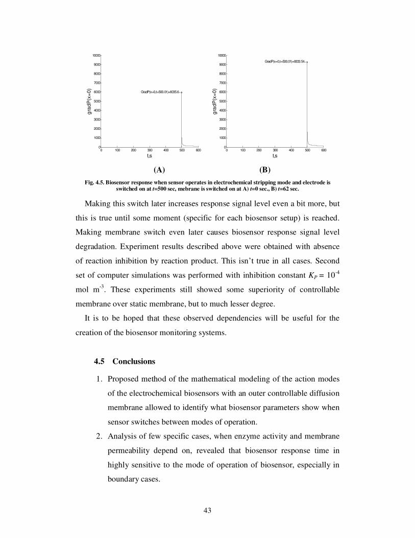
Fig. 4.5. Biosensor response when sensor operates in electrochemical stripping mode and electrode is switched on at t=500 sec, mebrane is switched on at A) t=0 sec., B) t=62 sec.

Making this switch later increases response signal level even a bit more, but

this is true until some moment (specific for each biosensor setup) is reached.

Making membrane switch even later causes biosensor response signal level

degradation. Experiment results described above were obtained with absence

of reaction inhibition by reaction product. This isn’t true in all cases. Second

set of computer simulations was performed with inhibition constant KP = 10-4

mol m-3. These experiments still showed some superiority of controllable

membrane over static membrane, but to much lesser degree.

It is to be hoped that these observed dependencies will be useful for the

creation of the biosensor monitoring systems.

4.5 Conclusions

1. Proposed method of the mathematical modeling of the action modes

of the electrochemical biosensors with an outer controllable diffusion

membrane allowed to identify what biosensor parameters show when

sensor switches between modes of operation.

2. Analysis of few specific cases, when enzyme activity and membrane

permeability depend on, revealed that biosensor response time in

highly sensitive to the mode of operation of biosensor, especially in

boundary cases.

44

3. Setting biosensor to deep diffusion mode allows achieving of

biosensor linear range expansion by several magnitudes.

4. Sensor could be easily switched to deep diffusion mode when

membrane permeability nonlinearly depends on medium pH and

permeability maximum is different from enzyme activity maximum.

5. Proposed and analyzed biosensor operating with controllable in time

permeability membrane yields higher response signal level compared

to biosensor with static membrane, when both biosensors are working

in electrochemical stripping regime, membrane of the first biosensor

is turned on at the selected moment of time, enzymatic reaction

inhibition by reaction product is low.

45

5 Conclusions

Basing on the results of the computer modeling of three biosensors with

innovative structure the following main conclusions were made:

1. Model described by [Verger72] cannot be applied directly for

Thermomyces lanuginosus lipase activity assessing biosensor.

Constant substrate concentration cannot be assumed thus model

should be extended with substrate kinetic equation. Such model

extension allows obtaining good fit between experimental and

computer simulation results. This computer modeling additionally

allows to evaluate enzymatic reaction rate constant.

2. According to the results of lipase activity assessment biosensor (with

substrate covered electrode) study, experimental data exhibit two

distinct types of substrate concentration decay: one exponential (in

respect to time) and the other of t-1-type. This indicates that, in the

dU/dt differential equation in system Eq (3.4), first and second order

(in respect to the substrate concentration) terms are competing and

should be taken into account in numeric modeling. Good fit between

experimental and computer simulation results could be obtained

when both terms are taken into account.

3. Biosensor with controllable permeability membrane could be easily

switched to deep diffusion mode when membrane permeability

nonlinearly depends on medium pH and permeability maximum is

different from enzyme activity maximum.

4. Biosensor operating with controllable in time permeability membrane

yields higher response signal level compared to biosensor with static

membrane, when both biosensors are working in electrochemical

stripping regime, membrane of the first biosensor is turned on at the

46

selected moment of time, enzymatic reaction inhibition by reaction

product is low.

47

6 Rerefences

[Bard01] A. J. Bard, L. R. Faulkner, Electrochemical Methods:

Fundamentals and Applications, second ed., Wiley, New York,

2001.

[Baron02] R. Baronas, F. Ivanauskas, J. Kulys, Modelling dynamics of

amperometric biosensors in batch and flow injection analysis.

J. Math. Chem. 32, 225-237, 2002.

[Baron03] R. Baronas, F. Ivanauskas, J. Kulys, and M. Sapagovas,

Modelling of amperometric biosensors with rough surface of

the enzyme membrane. J. Math. Chem., 34, 227, 2003.

[Baron04] R. Baronas, J. Kulys, F. Ivanauskas, Modelling

amperometric enzyme electrode with substrate cyclic

conversion. Biosens. Bioelectron., 19, 915, 2004.

[Beiss00] F. Beisson, A. Tiss, C. Riviere, R. Verger, Methods for

lipase detection and assay: a critical review. Eur. J. Lipid Sci.

Technol., 133-153, 2000.

[Blum91] L. J. Blum, P. R. Coulet, Biosensor Principles and

Applications, CRC Press, 1991.

[Born99] U.T. Bornscheuerand, R.J. Kazlauskas, Hydrolases in

Organic Synthesis Regio- and Stereoselective

Biotransformations, Wiley-VCH: Weinheim, 1999.

[Coop04] J. Cooper, A. E. G. Cass, Biosensors: A Practical Approach,

Oxford University Press, 2004.

[Frey07] P. A. Frey, A. D. Hegeman, Enzymatic Reaction

Mechanisms, Oxford University Press, Oxford, 2007.

48

[Houde04] A. Houde, A. Kademi, D. Leblanc, Lipases and their

industrial applications, Appl. Biochem. Biotechnol., 118(1–3),

pp. 155–170, 2004.

[Ignat05] I. Ignatjev, G. Valinčius, I. Švedait÷, E. Gaidamauskas, M.

Kažem÷kait÷, V. Razumas, A. Svendsen, Direct amperometric

determination of lipase activity, Anal. Biochem., 344(2), pp.

275–277, 2005.

[Kanap92] J.J. Kanapienene, A.A. Dedinaite and V. Laurinavicius,

Sens. & Actuators B. 10, 37, 1992.

[Kulys86] J. Kulys, V.V. Sorochinski and R.A. Vidziunaite, Transient

response of bienzyme electrodes. Biosensors, 2, 135, 1986.

[Laurin04] V. Laurinavicius, J. Razumiene, A. Ramanavicius, A.D.

Ryabov, Biosens. Bioelectron. 20, 1217, 2004.

[Laurin89] V.A. Laurinavicius, J.J. Kulys, V.V. Gureviciene and K.J.

Simonavicius, Biomed. Biochim. Acta. 48, 905, 1989.

[Mell75] L.D. Mell and J.T. Maloy, A model for the amperometric

enzyme electrode obtained through digital simulation and

applied to the glucose oxidase system. Anal. Chem., 47, 299,

1975.

[Puida07] M. Puida, F. Ivanauskas, I. Ignatjev, G. Valinčius, V.

Razumas, Computational modeling of the amperometric

bioanalytical system for lipase activity assay: a time-dependent

response. Nonlinear Analysis: Modelling and Control, 12 (3),

245–251, 2007.

[Puida08] M. Puida, F. Ivanauskas, I. Ignatjev, G. Valincius, V.

Razumas, Computational modeling of the electrochemical

system of lipase activity detection. Sensors, 8 (6), 2008.

[Samar01] A. A. Samarskii, The Theory of Difference Schemes, Marcel

49

Dekker, New York-Basel, 2001.

[Schell92] F. Scheller, F. Schubert, Biosensors, Elsevier, 1992.

[Schmi98] R. D. Schmid, R. Verger, Lipases: Interfacial enzymes with

attractive applications, Angew. Chem. Int. Ed., 37(12), pp.

1608–1633, 1998.

[Schul97] T. Schulmeister, J. Rose and F. Scheller, Mathematical

modelling of exponential amplification in membrane-based

enzyme sensors. Biosens. Bioelectron. 12, 1021, 1997.

[Shimi88] T. Shimidzu, A. Ohtani, K. Honda, Charge-previous

termcontrollablenext term poly pyrrole/poly electrolyte

composite previous termmembranes.next term Part III.

Electrochemical deionization system constructed by anion-

exchangeable and cation-exchangeable polypyrrole electrodes,

J. Electroanal. Chem., 251, 1988.

[Tran93] M. C. Tran, S. A. Jackson, Biosensors, Springer, 1993.

[Turner87] A.P.F. Turner, I. Karube and G.S. Wilson, Biosensors:

Fundamentals and Applications, Oxford University Press,

Oxford, 1987.

[Valin05] G. Valincius, I. Ignatjev, G. Niaura, M. Kažem÷kait÷, Z.

Talakait÷, V. Razumas, A. Svendsen, Electrochemical method

for the detection of lipase activity. Anal. Chem. 2005, 77 (8),

2632-2636.

[Verger72] R. Verger, M. C. E. Mieras, G. H. De Haas, Action of

phospholipase A at interfaces, J. Biol. Sci., 248(11), pp. 4023–

4034, 1972.R. Verger, M. C. E. Mieras, G. H. De Haas, Action

of phospholipase A at interfaces, J. Biol. Sci., 248(11), pp.

4023–4034, 1972.

[Yang06] G. Z. Yang, M. Yacoub, Body Sensor Networks, Birkhäuser,

50

2006

[Yu06] B. Yu, N. Long, Y. Moussy, F. Moussy, A long-term

flexible minimally-invasive implantable glucose biosensor

based on an epoxy-enhanced polyurethane membrane,

Biosensors and Bioelectronics, 21 (12), 2006.

51

List of publications

1. M. Puida, F. Ivanauskas, I. Ignatjev, G. Valinčius, V. Razumas,

Computational modeling of the amperometric bioanalytical system

for lipase activity assay: a time-dependent response. Nonlinear

Analysis: Modelling and Control, 12 (3), p. 245–251, 2007.

2. M. Puida, F. Ivanauskas, I. Ignatjev, G. Valincius, V. Razumas,

Computational modeling of the electrochemical system of lipase

activity detection, Sensors, 8 (6), p. 3873-3879, 2008.

3. M. Puida, F. Ivanauskas, V. Laurinavicius, Mathematical modeling

of the action of biosensor possessing variable parameters, (accepted

for publishing in Journal of Mathematical Chemistry on 17th April,

2009).

52

Curriculam vitae

Name: Mantas Puida Address: Department of Computer Science, Vilnius University, Naugarduko St. 24, LT-03225, Vilnius Phone: +370 682 43486 E-mail: [email protected] Education:

2002 B. Sc., Informatics, Kaunas University of Technology 2004 M. Sc., Informatics, Kaunas University of Technology 2004-2008 Doctoral studies, Vilnius university

53

Rezium÷

Kompiuterinis modeliavimas yra svarbus įrankis, kuriant naujus ir

tobulinant esamus biojutiklius. Tai tyrimo metodas, padedantis greitai ir

efektyviai ištirti, kokiomis savyb÷mis pasižym÷s naujai sukurti biojutikliai,

kokie procesai vyks juose ir kokie parametrai labiausiai lems šių jutiklių

atsaką. Šis metodas, sumažindamas fizinių eksperimentų poreikį iki

minimumo, padeda taupyti fizinius ir žmogiškuosius resursus. Biojutikliai yra

jautrūs, maži ir greiti analitiniai prietaisai, kasdien vis plačiau taikomi tokiose

srityse, kaip sveikatos priežiūra, aplinkosauga, maisto, popieriaus, tirpiklių

pramon÷. Struktūrin÷s ir kitos šių jutiklių inovacijos padeda pl÷sti jų taikymo

sritis bei gerinti jų analitines savybes. Kompiuterinis modeliavimas yra

priemon÷, kuri padeda iš anksti nusp÷ti, koks bus biojutiklio atsakas

konkrečiomis aplinkos sąlygomis, koks bus jo jautrumas, jautrumo ribos ar

greitaveika, kitaip tariant, padeda numatyti kiek praktiška būtų šio jutiklio

gamyba.

Šiame darbe nagrin÷jami trys struktūriniu požiūriu inovatyvūs biojutikliai:

lipaz÷s aktyvumo nustatymo biojutiklis su substratu, ištirpintu micel÷se,

lipaz÷s aktyvumo nustatymo biojutiklis su substratu, padengtu elektrodu bei

teorinis biojutiklis su valdomo laidumo (pavyzdžiui, keičiant terp÷s pH)

membrana. Šio darbo tikslai buvo parinkti tinkamus matematinius modelius šių

jutiklių kompiuteriniam modeliavimui. Taikant kompiuterinį modeliavimą,

siekta ištirti koks bus šių biojutiklių atsakas tam tikromis aplinkos sąlygomis,

kokie vidiniai bei išoriniai parametrai labiausiai lemia jų atsaką.

Šių biojutiklių tyrimui sukurta tokio tipo biojutiklių modeliavimą

automatizuojantis programin÷s įrangos paketas veikiantis Matlab aplinkoje.

Kompiuterinio modeliavimo būdu nustatyta, kad modeliuojant lipaz÷s

aktyvumo nustatymo biojutiklį su substratu, ištirpintu micel÷se, negalima

daryti prielaidos, jog viso eksperimento metu substrato koncentracija išlieka

pastovi, ir modelis turi būti papildytas substrato kinetine lygtimi. Taip pat

54

nustatyta fermentin÷s reakcijos greičio konstanta. Ištirta, kad papildomo

difuzinio sluoksnio įvedimas (kitus sluoksnius išlaikant tokio pat storio)

sumažina pradinį sistemos atsaką, o difuzinio sluoksnio siaurinimas didina

sistemos atsaką.

Kompiuterinio modeliavimo būdu nustatyta, kad klasikinis modelis tinka

paaiškinti tik daliai lipaz÷s aktyvumo nustatymo biojutiklio su substratu

padengtu elektrodu eksperimentinių duomenų. Taip pat tyrimai parod÷, kad

papildomos tarpin÷s būsenos įvedimas į fermentin÷s reakcijos mechanizmą

negali paaiškinti dalies fizinio eksperimento duomenų. Ištyrus fizinio

eksperimento duomenis pseudologaritmin÷se bei atvirkštin÷se skal÷se padaryta

prielaida, kad substrato kinetin÷je lygtyje gali konkuruoti du nariai (pirmos ir

antros eil÷s substrato atžvilgiu). Netiesiniu antros eil÷s substrato atžvilgiu

nusiplovimo nariu papildžius substrato kinetinę lygtį, gautas geras fizinio ir

skaitinio eksperimento duomenų sutapimas. Šis netipiškas nusiplovimo narys

gali būti paaiškintas tuo, kad elektrodas yra padengtas vos keliais substrato

sluoksniai, kurie susirišę tarpusavyje bei su elektrodu skirtingo stiprumo

ryšiais: stipresnis ryšys - substratas-elektrodas bei silpnesnis ryšys - substratas-

substratas. Tokiu atveju substrato nusiplovimo greitis būtų proporcingas

substrato koncentracijai ir tiesiškai su ja maž÷tų nuo didelio (kai vyrauja

substratas-substratas nusiplovimas) iki mažo (kai vyrauja substratas-elektrodas

nusiplovimas), o visas šis sud÷tingas procesas būtų matomas kaip antros eil÷s

nusiplovimo narys.

Kompiuterinio modeliavimo būdu nustatyta, kad biojutiklio atsako

nusistov÷jimo laikas itin jautrus biojutiklio darbo režimui ir gali būti

naudojamas kaip indikatorius, norint nustatyti, ar jutiklis dirba kinetiniu ar

difuziniu režimu. Perjungiant jutiklį į gilų difuzinį režimą, jo tiesinio atsako

diapazoną galima išpl÷sti keliomis eil÷mis. Biojutiklis su valdoma membrana,

kurios laidumas netiesiškai priklauso nuo terp÷s pH, o jos laidumo

maksimumas nesutampa su fermento aktyvumo maksimumu, lengvai gali būti

perjungiama iš kinetinio režimo į difuzinį ir atvirkščiai. Jutikliui dirbant

elektrocheminio stripingo režimu su laike valdoma membrana, tinkamai

55

parenkant membranos įjungimo laiką, galima gauti žymiai stipresnį sistemos

atsaką, nei tuo atveju, jei jutiklis tur÷tų statinę membraną. Šis atsako

sustiprinimas ryškiausias, kai reakcijos produktas silpnai inhibuoja fermentinę

reakciją.

Documents

COMPUTER MODELING OF STRUCTURAL INNOVATIONS IN BIOSENSORS