Computer Systems Modelling

Sam HainesClare College, University of Cambridge

1st March 2015

About the Course

• 12 lectures• 3 supervisions• 2 exam questions (Papers 8 and 9)

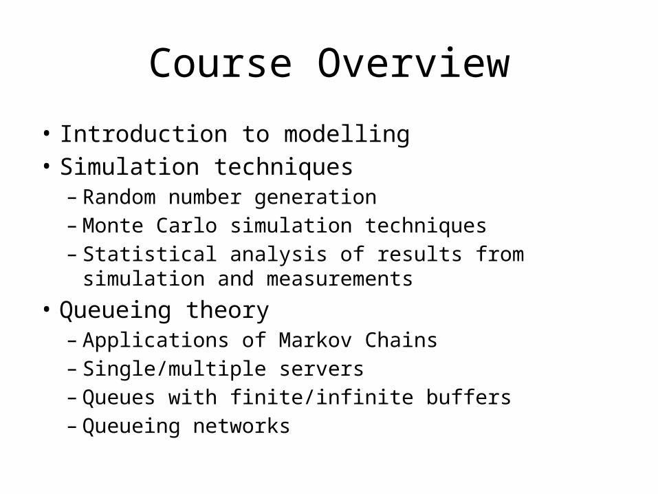
Course Overview

• Introduction to modelling• Simulation techniques

– Random number generation– Monte Carlo simulation techniques– Statistical analysis of results from simulation and

measurements• Queueing theory

– Applications of Markov Chains– Single/multiple servers– Queues with finite/infinite buffers– Queueing networks

Why model?

• Fundamental design decisions to help quantify a cost/benefit analysis

• A system is performing poorly – which problem should be tackled first?

• How long will a database request wait for before receiving CPU service?

• What is the utilization of a resource?

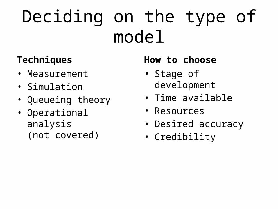
Deciding on the type of model

Techniques• Measurement• Simulation• Queueing theory• Operational analysis

(not covered)

How to choose• Stage of development• Time available• Resources• Desired accuracy• Credibility

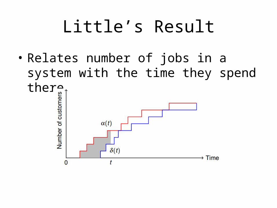
Little’s Result

• Relates number of jobs in a system with the time they spend there

Little’s Result (contd.)

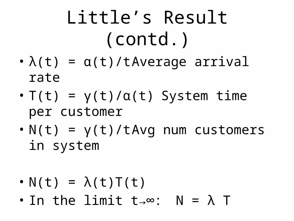
• λ(t) = α(t)/t Average arrival rate• T(t) = γ(t)/α(t) System time per customer• N(t) = γ(t)/t Avg num customers in system

• N(t) = λ(t)T(t)• In the limit t→∞: N = λ T

Recap from MMfCS

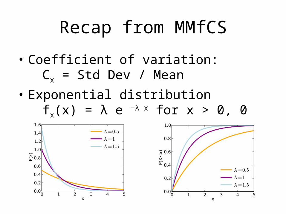
• Coefficient of variation:Cx = Std Dev / Mean

• Exponential distributionfx(x) = λ e −λ x for x > 0, 0 otherwise

Memoryless Property

• Exponential distribution is the only distribution with the Memoryless property

• P(X > t+s | X > t) = P(X > s)

• Intuitively, its used to model the inter-event times in which the time until the next event does not depend on the time that has already elapsed

• If inter-event times are IID RVs with Exp(λ),then λ is the mean event rate

Poisson Process

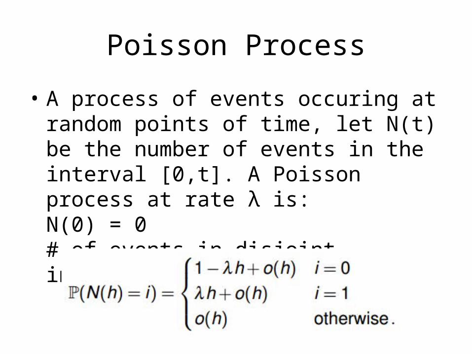
• A process of events occuring at random points of time, let N(t) be the number of events in the interval [0,t]. A Poisson process at rate λ is:N(0) = 0# of events in disjoint intervals is independent

Poisson Process (contd.)

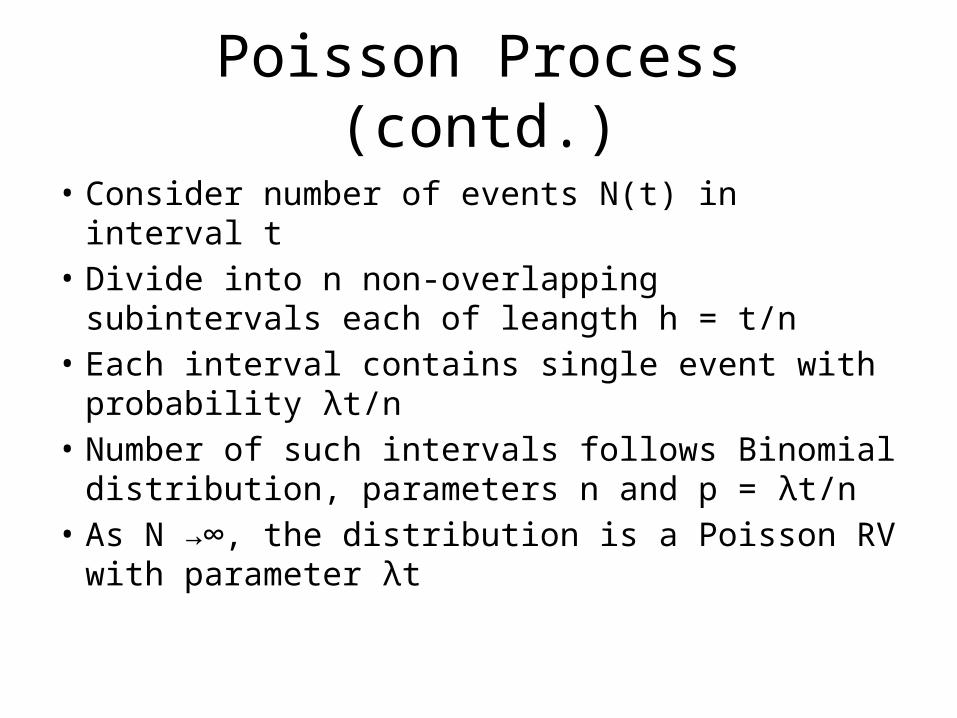
• Consider number of events N(t) in interval t• Divide into n non-overlapping subintervals each

of leangth h = t/n• Each interval contains single event with

probability λt/n• Number of such intervals follows Binomial

distribution, parameters n and p = λt/n• As N →∞, the distribution is a Poisson RV

with parameter λt

Poisson Process (contd.)

• For a Poisson process, let Xn be the time between the (n-1)st and nth events

• The sequence X1, X2,... gives the sequence of inter-event times

• P(X1 > t) = P(N(t) = 0) = e-λt

• So X1 (and hence the inter-event times) are random variables with Exp(λ)

Exam Question Structure

• Typically broken down into many smaller sections, each worth between 2 and 5 marks

• Typically one question each on:– Queueing– Simulation

Any Question

s?

Pub?