Embed Size (px)
Citation preview
Computer Aided Geometric Design 25 (2008) 503–522
Contents lists available at ScienceDirect
Computer Aided Geometric Design
www.elsevier.com/locate/cagd
Approximate convex decomposition of polyhedra and its applications
Jyh-Ming Lien a,∗, Nancy M. Amato b
a Department of Computer Science, George Mason University, USAb Department of Computer Science, Texas A&M University, USA
a r t i c l e i n f o a b s t r a c t
Article history:Received 21 August 2007Received in revised form 9 May 2008Accepted 9 May 2008Available online 17 June 2008
PACS:02.40.Dr
Keywords:Concavity measurementConvex decompositionFeature grouping
Decomposition is a technique commonly used to partition complex models into simplercomponents. While decomposition into convex components results in pieces that are easyto process, such decompositions can be costly to construct and can result in representationswith an unmanageable number of components. In this paper we explore an alternativepartitioning strategy that decomposes a given model into “approximately convex” piecesthat may provide similar benefits as convex components, while the resulting decompositionis both significantly smaller (typically by orders of magnitude) and can be computed moreefficiently. Indeed, for many applications, an approximate convex decomposition (acd) canmore accurately represent the important structural features of the model by providinga mechanism for ignoring less significant features, such as surface texture. We describea technique for computing acds of three-dimensional polyhedral solids and surfaces ofarbitrary genus. We provide results illustrating that our approach results in high qualitydecompositions with very few components and applications showing that comparableor better results can be obtained using acd decompositions in place of exact convexdecompositions (ecd) that are several orders of magnitude larger.
© 2008 Elsevier B.V. All rights reserved.
1. Introduction
One common strategy for dealing with large, complex models is to decompose them into components that are easierto process. Many different decomposition methods have been proposed—see, e.g., Chazelle and Palios (1994) for a briefreview of some common strategies. Of these, decomposition into convex components has been of great interest becausemany algorithms, such as collision detection and mesh generation, perform more efficiently on convex objects. Convexdecomposition of polygons is a well studied problem and has optimal solutions under different criteria; see Keil (2000)for a good survey. In contrast, convex decomposition in three-dimensions is far less understood and, despite the practicalmotivation, little research on convex decomposition of polyhedra has gone beyond the theoretical stage (Chazelle et al.,1995).
A major reason that convex decompositions of polyhedra are not used more extensively is that they are not practicalfor complex models—an exact convex decomposition (ecd) (Chazelle, 1981; Chazelle et al., 1995) can be costly to constructand can result in a representation with an unmanageable number of components. This is true for both solid decompositions(Chazelle, 1981), which consist of a collection of convex volumes whose union equals the original polyhedron, and surfacedecompositions (Chazelle et al., 1995), which partition the surface of the polyhedron into a collection of convex surfacepatches. For example, a solid ecd of the Armadillo model has more than 726 240 components and a surface ecd of theDavid model has 85 132 components (see Fig. 1). Similar statistics for additional models are show in Table 1 in Section 6.
* Corresponding author at: MSN 4A5, 4400 University Drive, Fairfax, Virginia, 22030, USA. Tel.: +1 703 993 9546.E-mail addresses: [email protected] (J.-M. Lien), [email protected] (N.M. Amato).
0167-8396/$ – see front matter © 2008 Elsevier B.V. All rights reserved.doi:10.1016/j.cagd.2008.05.003
504 J.-M. Lien, N.M. Amato / Computer Aided Geometric Design 25 (2008) 503–522
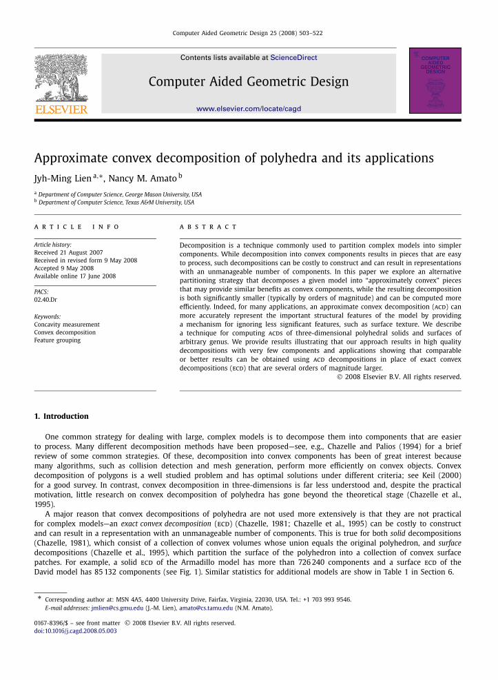
Fig. 1. The approximate convex decompositions (acd) of the Armadillo and the David models consist of a small number of nearly convex components thatcharacterize the important features of the models better than the exact convex decompositions (ecd) that have orders of magnitude more components. TheArmadillo model (500 K edges, 12.1 MB) has a solid acd with 98 components (14.2 MB) that can be computed in 232 seconds while the solid ecd has morethan 726 240 components (20+ GB) and could not be completed because the disk space was exhausted after nearly 4 hours of computation. The Davidmodel (750 K edges, 18 MB) has a surface acd with 66 components (18.1 MB) while the surface ecd has 85 132 components (20.1 MB).
1.1. An overview of our approach
In this work, we explore a partitioning strategy that decomposes a polyhedron into “approximately convex” pieces. Ourmotivation is that for many applications, the approximately convex components of this decomposition provide similar ben-efits as convex components, while the resulting decomposition is both significantly smaller (typically by several orders ofmagnitude) and can be computed more efficiently. These advantages have been proven theoretically and experimentally forplanar polygons in our previous work (Lien and Amato, 2004). In this paper we show that, unlike ecd, it is feasible to applythe concept of approximate convex decomposition (acd) to three-dimensional polyhedra. In particular, we describe
• practical methods for computing a solid or surface acd of a polyhedron of arbitrary genus.
Our general strategy is to iteratively identify the most concave feature(s) in the current decomposition, and then to par-tition the polyhedron so that the concavity of the identified features is reduced. This process continues until all componentsin the decomposition have acceptable concavity, i.e., until they are convex ‘enough’, which is a tunable parameter. Whilethis follows the general approach used successfully for polygons (Lien and Amato, 2004), there are several operations thatwere straight forward for polygons but which become nontrivial for polyhedra. The main challenges include computing theconcavity of a feature for a polyhedron and resolving concave features to generate small and high quality decomposition. Todeal with these technical challenges in 3D, we introduce a new technique:
• approximate feature grouping, that enables sets of features to be processed together, which is both more efficient andproduces better results.
We demonstrate the feasibility of our approach by applying it to a number of complex models. In general, even for verycomplex models, the acds have very few components, typically several orders of magnitude fewer than the ecds. The size(memory) and computational time are also significantly less, particularly for the solid acds; see Fig. 1.
We would like to emphasize that acd aims to provide an approximate representation of the original shape using aset of convex components. Thus, unlike the part-based segmentations using automatic (Rom and Medioni, 1994; Wu andLevine, 1997; Mangan and Whitaker, 1999; Li et al., 2001; Dey et al., 2003; Katz and Tal, 2003; Goswami et al., 2006;Lai et al., 2006) or (semi-)interactive (Funkhouser et al., 2004; Lee et al., 2005; Liu et al., 2006) approaches, the main goal ofacd is in fact closer to that of the work on shape approximation (Wu and Levine, 1994; Cohen-Steiner et al., 2004; Yamauchiet al., 2005). While most shape approximations focused on surfaces, acd provides both solid and surface approximations.
1.2. Applications of acd
In many applications, the detailed features of the model are not crucial and in fact considering them could serve toobscure important structural features and add to the processing cost. In such cases, an approximate representation of themodel, such as our proposed acd, that captures the key structural features would be preferable. For example, the acds ofthe Armadillo and the David models in Fig. 1 identify anatomical features much better than the ecds. Other applications ofacd include shape representation (Fig. 2), motion planning (Fig. 3), mesh generation (Fig. 4), and point location (Fig. 5).
J.-M. Lien, N.M. Amato / Computer Aided Geometric Design 25 (2008) 503–522 505
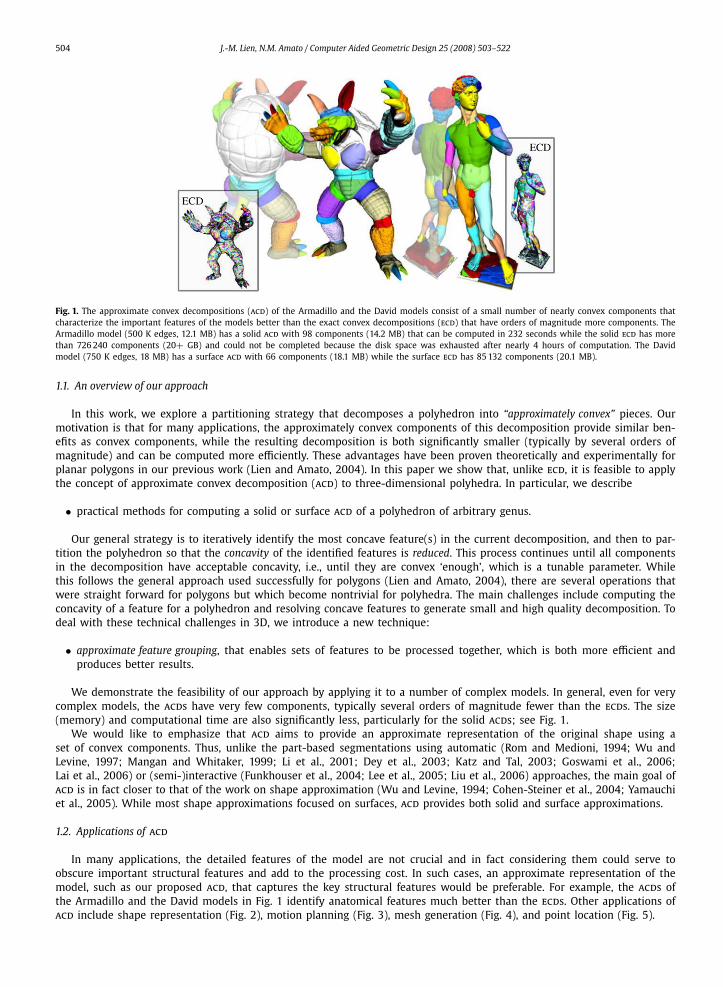
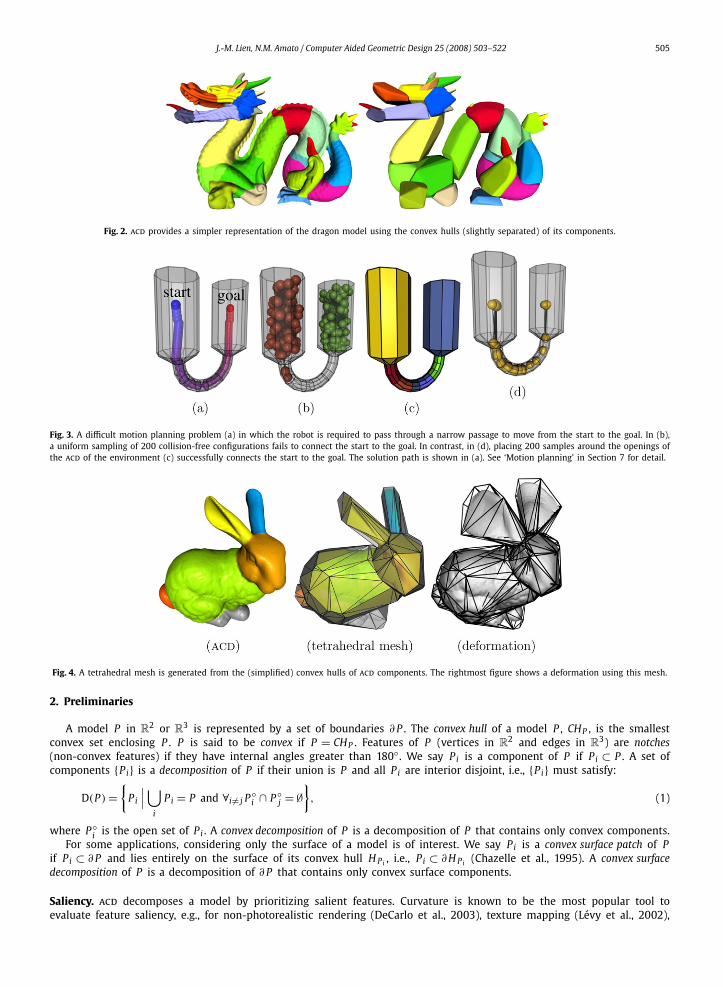
Fig. 2. acd provides a simpler representation of the dragon model using the convex hulls (slightly separated) of its components.
Fig. 3. A difficult motion planning problem (a) in which the robot is required to pass through a narrow passage to move from the start to the goal. In (b),a uniform sampling of 200 collision-free configurations fails to connect the start to the goal. In contrast, in (d), placing 200 samples around the openings ofthe acd of the environment (c) successfully connects the start to the goal. The solution path is shown in (a). See ‘Motion planning’ in Section 7 for detail.
Fig. 4. A tetrahedral mesh is generated from the (simplified) convex hulls of acd components. The rightmost figure shows a deformation using this mesh.
2. Preliminaries
A model P in R2 or R
3 is represented by a set of boundaries ∂ P . The convex hull of a model P , CHP , is the smallestconvex set enclosing P . P is said to be convex if P = CHP . Features of P (vertices in R
2 and edges in R3) are notches
(non-convex features) if they have internal angles greater than 180◦ . We say Pi is a component of P if Pi ⊂ P . A set ofcomponents {Pi} is a decomposition of P if their union is P and all Pi are interior disjoint, i.e., {Pi} must satisfy:
D(P ) ={
Pi
∣∣∣ ⋃i
P i = P and ∀i �= j P ◦i ∩ P ◦
j = ∅}, (1)
where P ◦i is the open set of Pi . A convex decomposition of P is a decomposition of P that contains only convex components.
For some applications, considering only the surface of a model is of interest. We say Pi is a convex surface patch of Pif Pi ⊂ ∂ P and lies entirely on the surface of its convex hull H Pi , i.e., Pi ⊂ ∂ H Pi (Chazelle et al., 1995). A convex surfacedecomposition of P is a decomposition of ∂ P that contains only convex surface components.
Saliency. acd decomposes a model by prioritizing salient features. Curvature is known to be the most popular tool toevaluate feature saliency, e.g., for non-photorealistic rendering (DeCarlo et al., 2003), texture mapping (Lévy et al., 2002),
506 J.-M. Lien, N.M. Amato / Computer Aided Geometric Design 25 (2008) 503–522
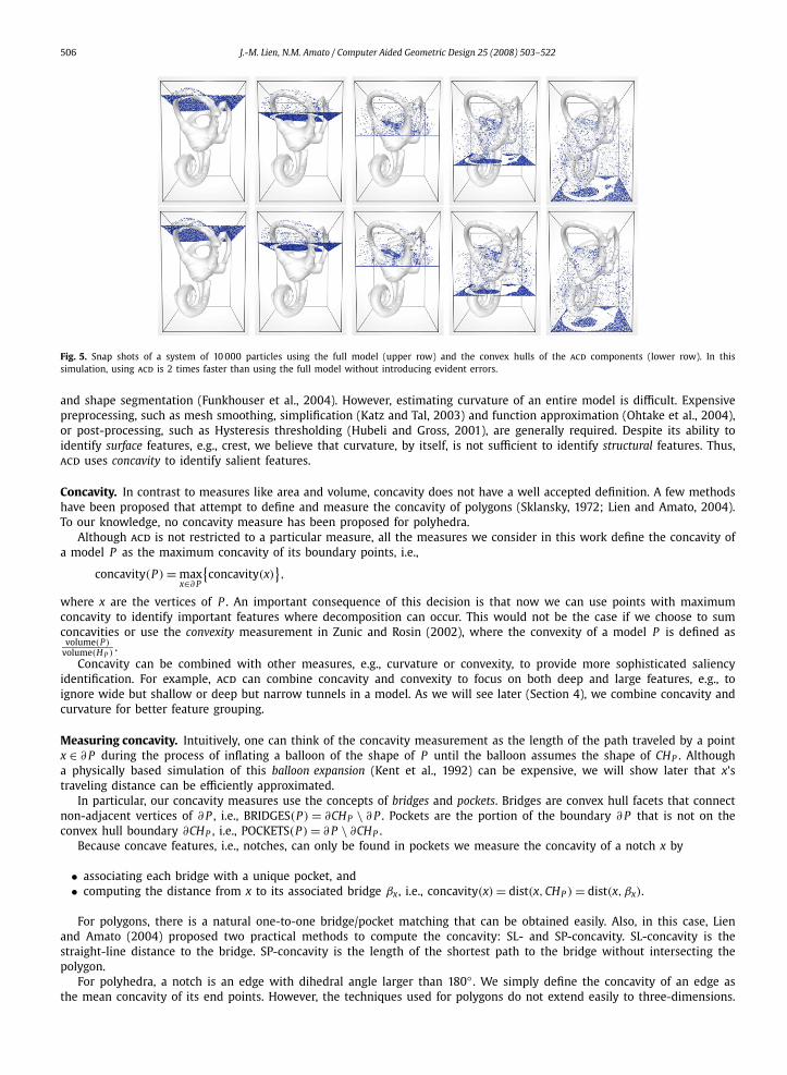
Fig. 5. Snap shots of a system of 10 000 particles using the full model (upper row) and the convex hulls of the acd components (lower row). In thissimulation, using acd is 2 times faster than using the full model without introducing evident errors.
and shape segmentation (Funkhouser et al., 2004). However, estimating curvature of an entire model is difficult. Expensivepreprocessing, such as mesh smoothing, simplification (Katz and Tal, 2003) and function approximation (Ohtake et al., 2004),or post-processing, such as Hysteresis thresholding (Hubeli and Gross, 2001), are generally required. Despite its ability toidentify surface features, e.g., crest, we believe that curvature, by itself, is not sufficient to identify structural features. Thus,acd uses concavity to identify salient features.
Concavity. In contrast to measures like area and volume, concavity does not have a well accepted definition. A few methodshave been proposed that attempt to define and measure the concavity of polygons (Sklansky, 1972; Lien and Amato, 2004).To our knowledge, no concavity measure has been proposed for polyhedra.
Although acd is not restricted to a particular measure, all the measures we consider in this work define the concavity ofa model P as the maximum concavity of its boundary points, i.e.,
concavity(P ) = maxx∈∂ P
{concavity(x)
},
where x are the vertices of P . An important consequence of this decision is that now we can use points with maximumconcavity to identify important features where decomposition can occur. This would not be the case if we choose to sumconcavities or use the convexity measurement in Zunic and Rosin (2002), where the convexity of a model P is defined as
volume(P )volume(H P )
.Concavity can be combined with other measures, e.g., curvature or convexity, to provide more sophisticated saliency
identification. For example, acd can combine concavity and convexity to focus on both deep and large features, e.g., toignore wide but shallow or deep but narrow tunnels in a model. As we will see later (Section 4), we combine concavity andcurvature for better feature grouping.
Measuring concavity. Intuitively, one can think of the concavity measurement as the length of the path traveled by a pointx ∈ ∂ P during the process of inflating a balloon of the shape of P until the balloon assumes the shape of CHP . Althougha physically based simulation of this balloon expansion (Kent et al., 1992) can be expensive, we will show later that x’straveling distance can be efficiently approximated.
In particular, our concavity measures use the concepts of bridges and pockets. Bridges are convex hull facets that connectnon-adjacent vertices of ∂ P , i.e., BRIDGES(P ) = ∂CHP \ ∂ P . Pockets are the portion of the boundary ∂ P that is not on theconvex hull boundary ∂CHP , i.e., POCKETS(P ) = ∂ P \ ∂CHP .
Because concave features, i.e., notches, can only be found in pockets we measure the concavity of a notch x by
• associating each bridge with a unique pocket, and• computing the distance from x to its associated bridge βx , i.e., concavity(x) = dist(x,CHP ) = dist(x, βx).
For polygons, there is a natural one-to-one bridge/pocket matching that can be obtained easily. Also, in this case, Lienand Amato (2004) proposed two practical methods to compute the concavity: SL- and SP-concavity. SL-concavity is thestraight-line distance to the bridge. SP-concavity is the length of the shortest path to the bridge without intersecting thepolygon.
For polyhedra, a notch is an edge with dihedral angle larger than 180◦ . We simply define the concavity of an edge asthe mean concavity of its end points. However, the techniques used for polygons do not extend easily to three-dimensions.
J.-M. Lien, N.M. Amato / Computer Aided Geometric Design 25 (2008) 503–522 507
In particular, there is no trivial one-to-one bridge/pocket matching. In addition, while SL-concavity can still be computedefficiently, the best known methods for computing shortest paths on polyhedra require exponential time (Sharir and Schorr,1986). We will address these issues later in this paper.
3. Approximate convex decomposition
The goal of approximate convex decomposition (acd) is to generate decompositions whose components are approxi-mately convex. We estimate how convex a component is using the concavity of the component. For a given model P , P issaid to be τ -approximate convex if concavity(P ) < τ , where concavity(ρ) denotes the concavity measurement of ρ and τ isa tunable parameter denoting the non-concavity tolerance of the application. A τ -approximate convex decomposition of P ,ACDτ (P ), is defined as a decomposition that contains only τ -approximate convex components; i.e.,
ACDτ (P ) = {Pi
∣∣ Pi ∈ D(P ) and concavity(Pi) � τ}. (2)
Thus, an acd0 is simply an exact convex decomposition.Our general strategy for computing acds follows the approach for polygons. Briefly, an acd is generated by recursively
removing (resolving) concave features in order of decreasing significance, i.e., concavity, until all remaining components haveconcavity less than some desired bound. This strategy is outlined in Algorithm 1.
The two main operations required in Algorithm 1 for acd are:
• measuring the concavity of a feature(s), and• resolving specified concave feature(s).
The approach outlined above is the same strategy applied to compute acds for polygons (Lien and Amato, 2004). For agiven polygon P , the concavity of notches x of the polygon P are computed using SL- or SP-concavity described in Section 2.Then, a notch x is resolved by adding a diagonal from x to ∂ P such that the dihedral angle of x is less than 180◦ . Fig. 6shows an acd of a polygon.
3.1. Issue: Measuring concave features
acd measures the concavity as the distance from a feature to its associated bridge. Unfortunately, unlike polygons, thereis no trivial one-to-one bridge/pocket matching for polyhedra. The problem of obtaining the bridge/pocket relationship isclosely related to the problem of spherical (Praun and Hoppe, 2003) and simplical (Khodakovsky et al., 2003) parameteriza-tion. However, mesh parameterization is costly to compute. Polyhedron realization (Shapiro and Tal, 1998) that transforms
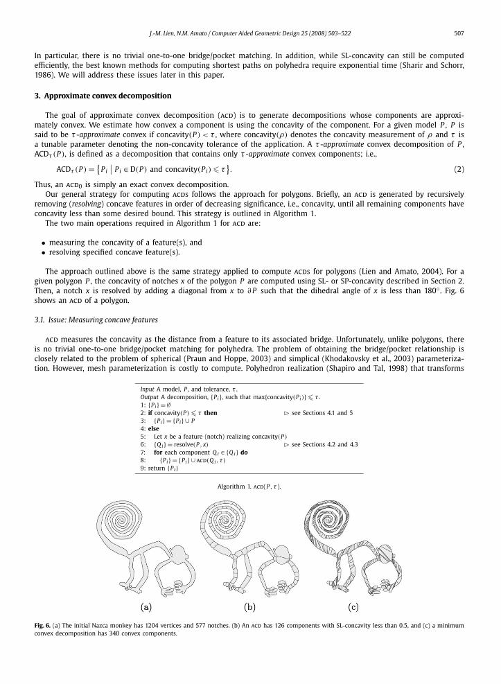
Input A model, P , and tolerance, τ .Output A decomposition, {Pi}, such that max{concavity(Pi)} � τ .1: {Pi} = ∅2: if concavity(P ) � τ then � see Sections 4.1 and 53: {Pi} = {Pi} ∪ P4: else5: Let x be a feature (notch) realizing concavity(P )
6: {Q i} = resolve(P , x) � see Sections 4.2 and 4.37: for each component Q i ∈ {Q i} do8: {Pi} = {Pi} ∪ acd(Q i , τ )
9: return {Pi}
Algorithm 1. acd(P , τ ).
Fig. 6. (a) The initial Nazca monkey has 1204 vertices and 577 notches. (b) An acd has 126 components with SL-concavity less than 0.5, and (c) a minimumconvex decomposition has 340 convex components.

508 J.-M. Lien, N.M. Amato / Computer Aided Geometric Design 25 (2008) 503–522
Fig. 7. Resolving concavity (a) using a cut plane that bisects a dihedral angle results in (b) a decomposition with 10 components with concavity � 0.1. Incontrast, (c) carefully selected cut planes generate only 4 components with concavity � 0.1.
a polyhedron P to a convex object H can be computed efficiently, but H is generally not the convex hull of P and cannotbe determined before performing the transformation. To address this difficulty, we propose a less expensive method that“projects” facets of ∂CHP to ∂ P instead of retracting ∂ P to ∂CHP .
As we mentioned earlier, while SL-concavity can still be computed efficiently, the best known methods for computingshortest paths on polyhedra require exponential time (Sharir and Schorr, 1986) and even methods (Choi et al., 1997) thatapproximate the shortest paths are too inefficient to be used in our approach. We use only SL-concavity in this paper.
3.2. Issue: Resolving concave features
Notch-cutting (Chazelle, 1981) is a strategy that splits a polyhedron with a cut plane. This strategy can be used to resolvenotches in Algorithm 1. The details of this notch-cutting strategy are discussed in (Bajaj and Dey, 1992). Figs. 7(a)(b) illustratean acd using cut planes that bisect dihedral angles.
A difficulty of this approach is selecting “good” cut planes. For example, in Fig. 7(c), carefully selected cut planes cangenerate fewer components than cut planes that simply bisect the dihedral angles of notches. Unfortunately, good strategiesfor finding such good cut planes are not well known. Joe (1994) proposed an approach to postpone processing notcheswhose resolution would produce small components, but this strategy still produces many small components with sharpedges for large models, especially for more complicated models that are commonly seen nowadays.
We address this difficulty by identifying concave features that can potentially be resolved together. Intuitively, these features area connected set of edges lying in highly concave areas.
3.3. General strategy: Feature grouping
To address issues of measuring and resolving concavities, we use a technique we call feature grouping to collect sets ofsimilar and adjacent features that can be processed together.
For measuring concavity, by allowing bridges to be formed from convex hull patches instead of a single convex hullfacet, we can both dramatically reduce the number of bridges as well as decrease the cost of computing the pocket tobridge matching. Fig. 8 shows an example of the bridge/pocket relationship with and without grouping. As we will see inSection 4.1, bridge patches can be used to provide a conservative measure of concavity.
Resolution of concavity can also be improved by considering feature sets rather than individual features and by forcingthe cut plane to be defined with respect to a feature set. Unlike the existing curvature-based methods (Hubeli and Gross,2001; DeCarlo et al., 2003; Ohtake et al., 2004; Rusinkiewicz, 2004; Yoshizawa et al., 2005), our feature grouping is basedon concavity.
4. ACD of polyhedra without handles
We first discuss our strategy for computing an acd of a genus zero polyhedron. This strategy will be extended to handlepolyhedra with non-zero genus in the next section.
4.1. Measuring concave features
Recall that we define the concavity of a vertex x as the distance from ∂ P to the convex hull boundary. Since there is nounambiguous mapping from notches to convex hull facets in 3D as there was in 2D, we first must define one.
Our strategy to match bridges with pockets is to identify pockets by projecting convex hull edges to the polyhedron’ssurface. The “projection” of a convex hull edge e is a path on the polyhedron’s surface ∂ P connecting the end points of e;we compute the paths on ∂ P using a modified Dijkstra’s algorithm. The main modification is to ensure that the paths foundon ∂ P do not cross each other. More specifically, we call Dijkstra’s algorithm twice for all convex hull edges. In the firstround, each path is independent thus may have intersections. The main goal of the first round is to estimate the lengthof each projection. In the second round, convex hull edges are projected in the order of estimated projection lengths from
J.-M. Lien, N.M. Amato / Computer Aided Geometric Design 25 (2008) 503–522 509
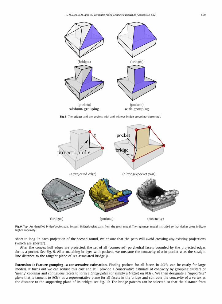
Fig. 8. The bridges and the pockets with and without bridge grouping (clustering).
Fig. 9. Top: An identified bridge/pocket pair. Bottom: Bridge/pocket pairs from the teeth model. The rightmost model is shaded so that darker areas indicatehigher concavity.
short to long. In each projection of the second round, we ensure that the path will avoid crossing any existing projections(which are shorter).
After the convex hull edges are projected, the set of all (connected) polyhedral facets bounded by the projected edgesforms a pocket. See Fig. 9. After matching bridges with pockets, we measure the concavity of x in pocket ρ as the straightline distance to the tangent plane of ρ ’s associated bridge β .
Extension 1: Feature grouping—a conservative estimation. Finding pockets for all facets in ∂CHP can be costly for largemodels. It turns out we can reduce this cost and still provide a conservative estimate of concavity by grouping clusters of‘nearly’ coplanar and contiguous facets to form a bridge patch (or simply a bridge) on ∂CHP . We then designate a “supporting”plane that is tangent to ∂CHP as a representative plane for all facets in the bridge and compute the concavity of a vertex asthe distance to the supporting plane of its bridge; see Fig. 10. The bridge patches can be selected so that the distance from
510 J.-M. Lien, N.M. Amato / Computer Aided Geometric Design 25 (2008) 503–522
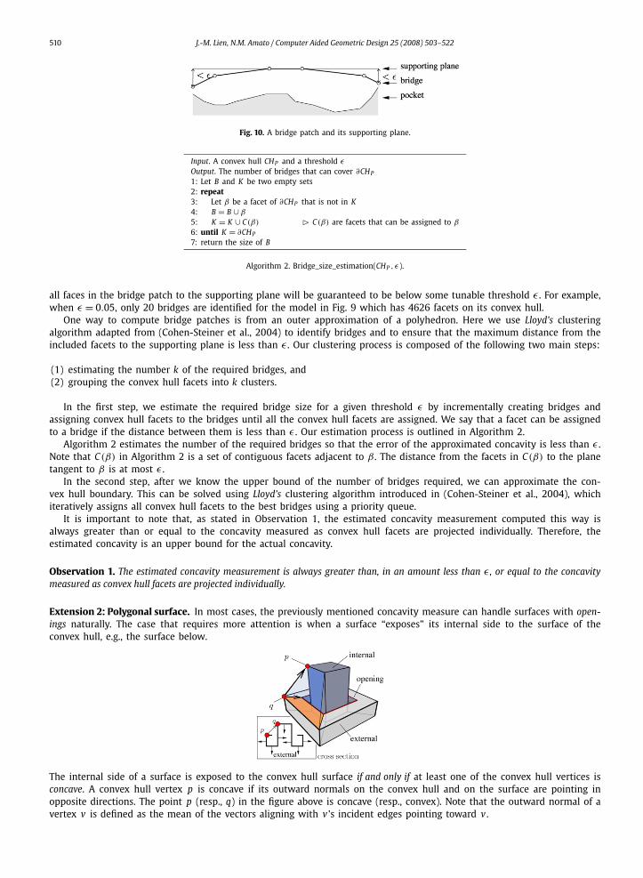
Fig. 10. A bridge patch and its supporting plane.
Input. A convex hull CHP and a threshold εOutput. The number of bridges that can cover ∂CHP
1: Let B and K be two empty sets2: repeat3: Let β be a facet of ∂CHP that is not in K4: B = B ∪ β
5: K = K ∪ C(β) � C(β) are facets that can be assigned to β
6: until K = ∂CHP
7: return the size of B
Algorithm 2. Bridge_size_estimation(CHP , ε).
all faces in the bridge patch to the supporting plane will be guaranteed to be below some tunable threshold ε . For example,when ε = 0.05, only 20 bridges are identified for the model in Fig. 9 which has 4626 facets on its convex hull.
One way to compute bridge patches is from an outer approximation of a polyhedron. Here we use Lloyd’s clusteringalgorithm adapted from (Cohen-Steiner et al., 2004) to identify bridges and to ensure that the maximum distance from theincluded facets to the supporting plane is less than ε . Our clustering process is composed of the following two main steps:
(1) estimating the number k of the required bridges, and(2) grouping the convex hull facets into k clusters.
In the first step, we estimate the required bridge size for a given threshold ε by incrementally creating bridges andassigning convex hull facets to the bridges until all the convex hull facets are assigned. We say that a facet can be assignedto a bridge if the distance between them is less than ε . Our estimation process is outlined in Algorithm 2.
Algorithm 2 estimates the number of the required bridges so that the error of the approximated concavity is less than ε .Note that C(β) in Algorithm 2 is a set of contiguous facets adjacent to β . The distance from the facets in C(β) to the planetangent to β is at most ε .
In the second step, after we know the upper bound of the number of bridges required, we can approximate the con-vex hull boundary. This can be solved using Lloyd’s clustering algorithm introduced in (Cohen-Steiner et al., 2004), whichiteratively assigns all convex hull facets to the best bridges using a priority queue.
It is important to note that, as stated in Observation 1, the estimated concavity measurement computed this way isalways greater than or equal to the concavity measured as convex hull facets are projected individually. Therefore, theestimated concavity is an upper bound for the actual concavity.
Observation 1. The estimated concavity measurement is always greater than, in an amount less than ε , or equal to the concavitymeasured as convex hull facets are projected individually.
Extension 2: Polygonal surface. In most cases, the previously mentioned concavity measure can handle surfaces with open-ings naturally. The case that requires more attention is when a surface “exposes” its internal side to the surface of theconvex hull, e.g., the surface below.
The internal side of a surface is exposed to the convex hull surface if and only if at least one of the convex hull vertices isconcave. A convex hull vertex p is concave if its outward normals on the convex hull and on the surface are pointing inopposite directions. The point p (resp., q) in the figure above is concave (resp., convex). Note that the outward normal of avertex v is defined as the mean of the vectors aligning with v ’s incident edges pointing toward v .
J.-M. Lien, N.M. Amato / Computer Aided Geometric Design 25 (2008) 503–522 511
Now, we can compute the pocket of a bridge β from the projection of β ’s boundary ∂β . Let e be an edge of ∂β . If e’svertices are
• both convex, then project e as before,• both concave, then e has no projection,• one convex and one concave (e.g., the edge pq in the figure), then e’s projection is the path connecting the convex end to
the opening.
4.2. Resolving concave features
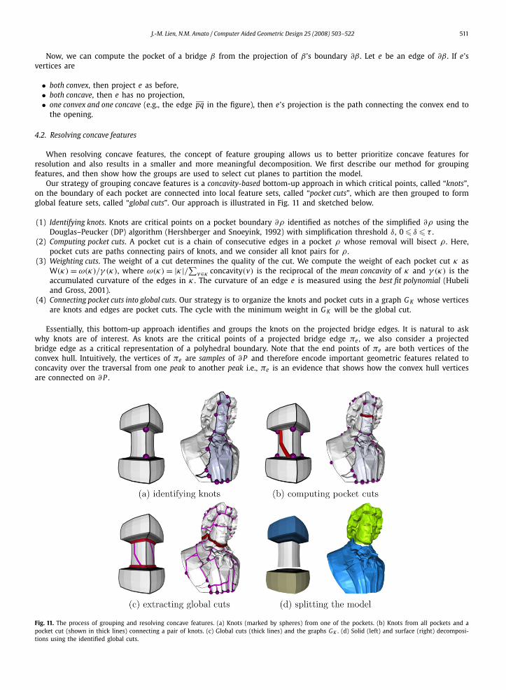
When resolving concave features, the concept of feature grouping allows us to better prioritize concave features forresolution and also results in a smaller and more meaningful decomposition. We first describe our method for groupingfeatures, and then show how the groups are used to select cut planes to partition the model.
Our strategy of grouping concave features is a concavity-based bottom-up approach in which critical points, called “knots”,on the boundary of each pocket are connected into local feature sets, called “pocket cuts”, which are then grouped to formglobal feature sets, called “global cuts”. Our approach is illustrated in Fig. 11 and sketched below.
(1) Identifying knots. Knots are critical points on a pocket boundary ∂ρ identified as notches of the simplified ∂ρ using theDouglas–Peucker (DP) algorithm (Hershberger and Snoeyink, 1992) with simplification threshold δ, 0 � δ � τ .
(2) Computing pocket cuts. A pocket cut is a chain of consecutive edges in a pocket ρ whose removal will bisect ρ . Here,pocket cuts are paths connecting pairs of knots, and we consider all knot pairs for ρ .
(3) Weighting cuts. The weight of a cut determines the quality of the cut. We compute the weight of each pocket cut κ asW(κ) = ω(κ)/γ (κ), where ω(κ) = |κ |/∑v∈κ concavity(v) is the reciprocal of the mean concavity of κ and γ (κ) is theaccumulated curvature of the edges in κ . The curvature of an edge e is measured using the best fit polynomial (Hubeliand Gross, 2001).
(4) Connecting pocket cuts into global cuts. Our strategy is to organize the knots and pocket cuts in a graph G K whose verticesare knots and edges are pocket cuts. The cycle with the minimum weight in G K will be the global cut.
Essentially, this bottom-up approach identifies and groups the knots on the projected bridge edges. It is natural to askwhy knots are of interest. As knots are the critical points of a projected bridge edge πe , we also consider a projectedbridge edge as a critical representation of a polyhedral boundary. Note that the end points of πe are both vertices of theconvex hull. Intuitively, the vertices of πe are samples of ∂ P and therefore encode important geometric features related toconcavity over the traversal from one peak to another peak i.e., πe is an evidence that shows how the convex hull verticesare connected on ∂ P .
Fig. 11. The process of grouping and resolving concave features. (a) Knots (marked by spheres) from one of the pockets. (b) Knots from all pockets and apocket cut (shown in thick lines) connecting a pair of knots. (c) Global cuts (thick lines) and the graphs G K . (d) Solid (left) and surface (right) decomposi-tions using the identified global cuts.
512 J.-M. Lien, N.M. Amato / Computer Aided Geometric Design 25 (2008) 503–522
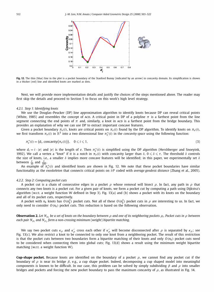
Fig. 12. The thin (blue) line in the plot is a pocket boundary of the Stanford Bunny (indicated by an arrow) in concavity domain. Its simplification is shownin a thicker (red) line and identified knots are marked as dots.
Next, we will provide more implementation details and justify the choices of the steps mentioned above. The reader mayfirst skip the details and proceed to Section 5 to focus on this work’s high level strategy.
4.2.1. Step 1: Identifying knotsWe use the Douglas–Peucker (DP) line approximation algorithm to identify knots because DP can reveal critical points
(White, 1985) and resembles the concept of acd. A critical point in DP of a polyline π is a farthest point from the linesegment connecting the end points of π and, similarly, a knot in acd is a farthest point from the bridge boundary. Thisprovides an explanation of why we can use DP to extract important concave features.
Given a pocket boundary πe(i), knots are critical points on πe(i) found by the DP algorithm. To identify knots on πe(i),we first transform πe(i) in R
3 into a two dimensional line π∗e (i) in the concavity space using the following function:
π∗e (i) = (
di, concavity(πe(i)
)), 0 � i � 1, (3)
where di = i · |e| and |e| is the length of e. Then π∗e (i) is simplified using the DP algorithm (Hershberger and Snoeyink,
1992). We call a vertex a “knot” if it is a notch in πe(i) with concavity larger than δ, 0 � δ � τ . The threshold δ controlsthe size of knots, i.e., a smaller δ implies more concave features will be identified; in this paper, we experimentally set δ
between τ10 and τ
100 .An example of π∗
e (i) and identified knots are shown in Fig. 12. We note that these pocket boundaries have similarfunctionality as the exoskeleton that connects critical points on ∂ P coded with average geodesic distance (Zhang et al., 2005).
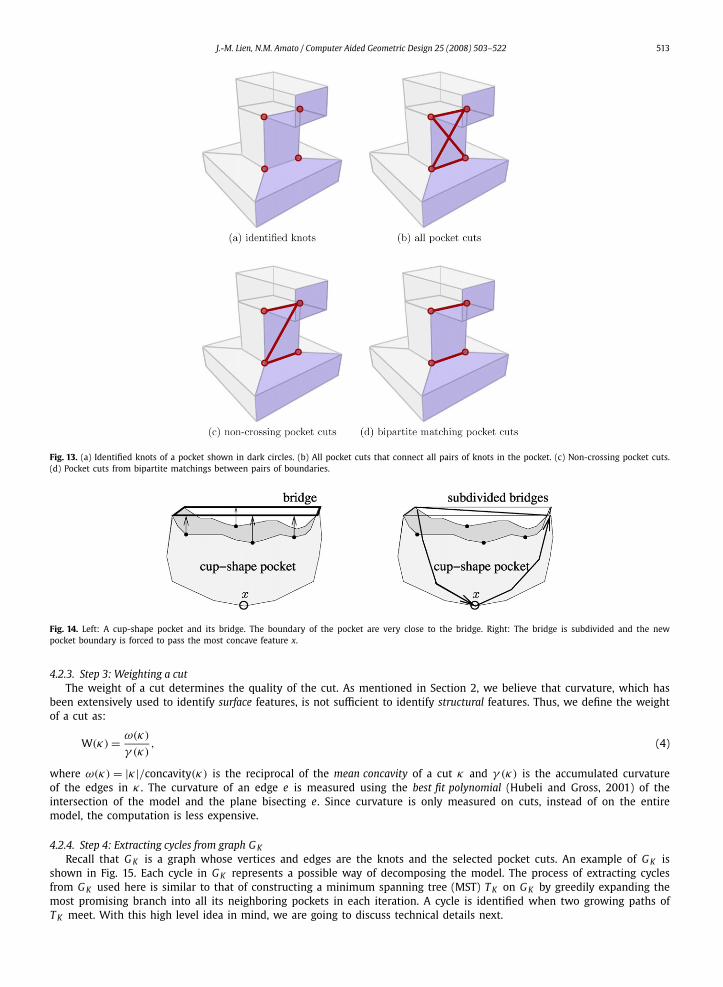
4.2.2. Step 2: Computing pocket cutsA pocket cut is a chain of consecutive edges in a pocket ρ whose removal will bisect ρ . In fact, any path in ρ that
connects any two knots is a pocket cut. For a given pair of knots, we form a pocket cut by computing a path using Dijkstra’salgorithm (w.r.t. a weight function W defined in Step 3). Fig. 13(a) and (b) shows a pocket with its knots on the boundaryand all of its pocket cuts, respectively.
A pocket with nk knots has O (n2k ) pocket cuts. Not all of these O (n2
k ) pocket cuts in ρ are interesting to us. In fact, weonly need to consider O (nk) pocket cuts. This reduction is based on the following observation.
Observation 2. Let Nρi be a set of knots on the boundary between ρ and one of its neighboring pockets ρi . Pocket cuts in ρ betweeneach pair Nρi and Nρ j form a non-crossing minimum (weight) bipartite matching.
We say two pocket cuts κρ and κ ′ρ cross each other if κ ′
ρ will become disconnected after ρ is separated by κρ ; seeFig. 13(c). We also restrict a knot to be connected to only one knot from a neighboring pocket. The result of this restrictionis that the pocket cuts between two boundaries form a bipartite matching of their knots and only O (nk) pocket cuts needto be considered when connecting them into global cuts; Fig. 13(d) shows a result using the minimum weight bipartitematching (w.r.t. a weight function W).
Cup-shape pocket. Because knots are identified on the boundary of a pocket ρ , we cannot find any pocket cut if theboundary of ρ is near its bridge β , e.g., a cup shape pocket. Indeed, decomposing a cup shaped model into meaningfulcomponents is known to be difficult. In our case, this problem can be solved by simply subdividing β and ρ into smallerbridges and pockets and forcing the new pocket boundary to pass the maximum concavity of ρ , as illustrated in Fig. 14.
J.-M. Lien, N.M. Amato / Computer Aided Geometric Design 25 (2008) 503–522 513
Fig. 13. (a) Identified knots of a pocket shown in dark circles. (b) All pocket cuts that connect all pairs of knots in the pocket. (c) Non-crossing pocket cuts.(d) Pocket cuts from bipartite matchings between pairs of boundaries.
Fig. 14. Left: A cup-shape pocket and its bridge. The boundary of the pocket are very close to the bridge. Right: The bridge is subdivided and the newpocket boundary is forced to pass the most concave feature x.
4.2.3. Step 3: Weighting a cutThe weight of a cut determines the quality of the cut. As mentioned in Section 2, we believe that curvature, which has
been extensively used to identify surface features, is not sufficient to identify structural features. Thus, we define the weightof a cut as:
W(κ) = ω(κ)
γ (κ), (4)
where ω(κ) = |κ |/concavity(κ) is the reciprocal of the mean concavity of a cut κ and γ (κ) is the accumulated curvatureof the edges in κ . The curvature of an edge e is measured using the best fit polynomial (Hubeli and Gross, 2001) of theintersection of the model and the plane bisecting e. Since curvature is only measured on cuts, instead of on the entiremodel, the computation is less expensive.
4.2.4. Step 4: Extracting cycles from graph G K
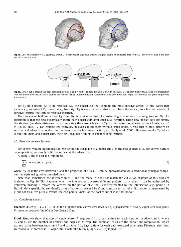
Recall that G K is a graph whose vertices and edges are the knots and the selected pocket cuts. An example of G K isshown in Fig. 15. Each cycle in G K represents a possible way of decomposing the model. The process of extracting cyclesfrom G K used here is similar to that of constructing a minimum spanning tree (MST) T K on G K by greedily expanding themost promising branch into all its neighboring pockets in each iteration. A cycle is identified when two growing paths ofT K meet. With this high level idea in mind, we are going to discuss technical details next.
514 J.-M. Lien, N.M. Amato / Computer Aided Geometric Design 25 (2008) 503–522
Fig. 15. Left: An example of G K (partially shown). Thicker pocket cuts have smaller weights. Right: An extracted tree from G K . The boldest line is the bestglobal cut for the root.
Fig. 16. Left: A cut κ around the neck connecting points a and b. Mid: The best fit plane E of κ . In this case, E is slightly higher than a and E ’s intersectionwith the model does not match κ . Lighter and darker shades indicate different components after decomposition. Right: An improved cut plane by pushingE towards a.
Let κρ be a pocket cut to be resolved, e.g., the pocket cut that contains the most concave vertex. To find cycles thatinclude κρ , we extract T K rooted at κρ from G K . T K is constructed so that a path from the root κρ to a leaf will consist ofconcave features that can be resolved together.
The process of building a tree T K from G K is similar to that of constructing a minimum spanning tree on G K . Anexception is that we also dynamically create new pocket cuts after each MST iteration. These new pocket cuts are simplythe shortest (geodesic distance) paths connecting the current leaves of T K to the pocket boundaries without knots, e.g., κ ′in Fig. 15. Thus, T K can explore low concavity or even convex areas without using knots. A MST that is built directly onvertices and edges of a polyhedron has been used for feature extraction, e.g. (Pauly et al., 2003). However, unlike T K whichis built on knots and pocket cuts, their MST requires pruning to enhance long features.
4.3. Resolving concave features
For convex volume decomposition, we define the cut plane of a global cut κ as the best fit plane of κ . For convex surfacedecomposition, we simply split the surface at the edges of κ .
A plane E fits κ best if E minimizes∑e∈κ
concavity(e) · μE(e), (5)
where μE(e) is the area between e and the projection of e to E . E can be approximated via a traditional principal compo-nent analysis using points sampled on κ .
Note that, sometimes, the intersection of E and the model P does not match the cut κ . An example of this problemis shown in Fig. 16. This happens when the intersection traverses different pockets that κ does. It can be addressed byiteratively pushing E toward the vertices on the portion of κ that is misrepresented by the intersection, e.g., point a inFig. 16. More specifically, we identify a set of pockets traversed by E and compare to that of κ . If a pocket is intersected byκ but not by E , we push E toward the end points (knots) of the pocket cut of κ in that pocket.
4.4. Complexity analysis
Theorem 3. Let {Ci}, i = 1, . . . ,m, be the τ -approximate convex decomposition of a polyhedron P with ne edges with zero genus.P can be decomposed into {Ci} in O (n3
e log ne) time.
Proof. First, we show that acd of a polyhedron P requires O (nvne log nv) time for each iteration in Algorithm 1, wherenv and ne are the number of vertices and edges in P , resp. The dominant costs are the pocket cut computation, whichextracts paths between knots on ∂ P and can take O (ne lognv ) time for each path extracted time using Dijkstra’s algorithm.To resolve all r notches in P , Algorithm 1 will take O (rnvne log nv) = O (n3
e log ne). �
J.-M. Lien, N.M. Amato / Computer Aided Geometric Design 25 (2008) 503–522 515
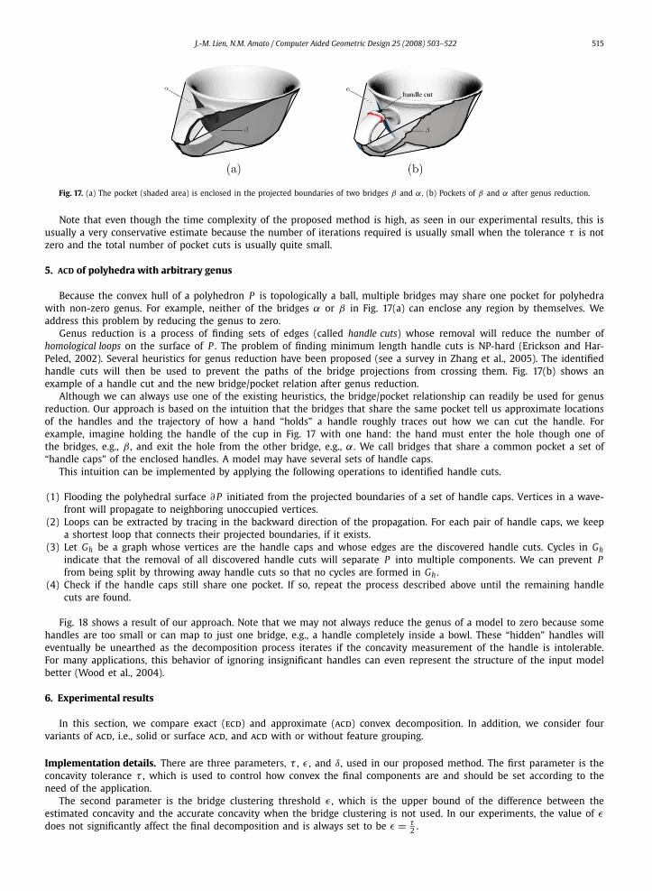
Fig. 17. (a) The pocket (shaded area) is enclosed in the projected boundaries of two bridges β and α. (b) Pockets of β and α after genus reduction.
Note that even though the time complexity of the proposed method is high, as seen in our experimental results, this isusually a very conservative estimate because the number of iterations required is usually small when the tolerance τ is notzero and the total number of pocket cuts is usually quite small.
5. ACD of polyhedra with arbitrary genus
Because the convex hull of a polyhedron P is topologically a ball, multiple bridges may share one pocket for polyhedrawith non-zero genus. For example, neither of the bridges α or β in Fig. 17(a) can enclose any region by themselves. Weaddress this problem by reducing the genus to zero.
Genus reduction is a process of finding sets of edges (called handle cuts) whose removal will reduce the number ofhomological loops on the surface of P . The problem of finding minimum length handle cuts is NP-hard (Erickson and Har-Peled, 2002). Several heuristics for genus reduction have been proposed (see a survey in Zhang et al., 2005). The identifiedhandle cuts will then be used to prevent the paths of the bridge projections from crossing them. Fig. 17(b) shows anexample of a handle cut and the new bridge/pocket relation after genus reduction.
Although we can always use one of the existing heuristics, the bridge/pocket relationship can readily be used for genusreduction. Our approach is based on the intuition that the bridges that share the same pocket tell us approximate locationsof the handles and the trajectory of how a hand “holds” a handle roughly traces out how we can cut the handle. Forexample, imagine holding the handle of the cup in Fig. 17 with one hand: the hand must enter the hole though one ofthe bridges, e.g., β , and exit the hole from the other bridge, e.g., α. We call bridges that share a common pocket a set of“handle caps” of the enclosed handles. A model may have several sets of handle caps.
This intuition can be implemented by applying the following operations to identified handle cuts.
(1) Flooding the polyhedral surface ∂ P initiated from the projected boundaries of a set of handle caps. Vertices in a wave-front will propagate to neighboring unoccupied vertices.
(2) Loops can be extracted by tracing in the backward direction of the propagation. For each pair of handle caps, we keepa shortest loop that connects their projected boundaries, if it exists.
(3) Let Gh be a graph whose vertices are the handle caps and whose edges are the discovered handle cuts. Cycles in Ghindicate that the removal of all discovered handle cuts will separate P into multiple components. We can prevent Pfrom being split by throwing away handle cuts so that no cycles are formed in Gh .
(4) Check if the handle caps still share one pocket. If so, repeat the process described above until the remaining handlecuts are found.
Fig. 18 shows a result of our approach. Note that we may not always reduce the genus of a model to zero because somehandles are too small or can map to just one bridge, e.g., a handle completely inside a bowl. These “hidden” handles willeventually be unearthed as the decomposition process iterates if the concavity measurement of the handle is intolerable.For many applications, this behavior of ignoring insignificant handles can even represent the structure of the input modelbetter (Wood et al., 2004).
6. Experimental results
In this section, we compare exact (ecd) and approximate (acd) convex decomposition. In addition, we consider fourvariants of acd, i.e., solid or surface acd, and acd with or without feature grouping.
Implementation details. There are three parameters, τ , ε , and δ, used in our proposed method. The first parameter is theconcavity tolerance τ , which is used to control how convex the final components are and should be set according to theneed of the application.
The second parameter is the bridge clustering threshold ε , which is the upper bound of the difference between theestimated concavity and the accurate concavity when the bridge clustering is not used. In our experiments, the value of εdoes not significantly affect the final decomposition and is always set to be ε = τ .
2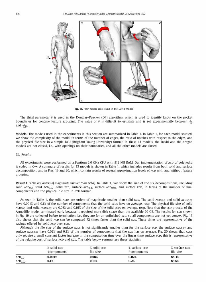
516 J.-M. Lien, N.M. Amato / Computer Aided Geometric Design 25 (2008) 503–522
Fig. 18. Four handle cuts found in the David model.
The third parameter δ is used in the Douglas–Peucker (DP) algorithm, which is used to identify knots on the pocketboundaries for concave feature grouping. The value of δ is difficult to estimate and is set experimentally between τ
10and τ
100 .
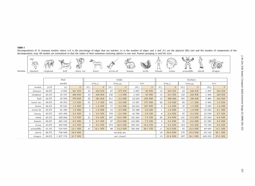
Models. The models used in the experiments in this section are summarized in Table 1. In Table 1, for each model studied,we show the complexity of the model in terms of the number of edges, the ratio of notches with respect to the edges, andthe physical file size in a simple BYU (Brigham Young University) format. In these 13 models, the David and the dragonmodels are not closed, i.e., with openings on their boundaries, and all the other models are closed.
6.1. Results
All experiments were performed on a Pentium 2.0 GHz CPU with 512 MB RAM. Our implementation of acd of polyhedrais coded in C++. A summary of results for 13 models is shown in Table 1, which includes results from both solid and surfacedecomposition, and in Figs. 19 and 20, which contain results of several approximation levels of acd with and without featuregrouping.
Result 1 (acds are orders of magnitude smaller than ecds). In Table 1, We show the size of the six decompositions, includingsolid acd0.2, solid acd0.02, solid ecd, surface acd0.2, surface acd0.02, and surface ecd, in terms of the number of finalcomponents and the physical file size in BYU format.
As seen in Table 1, the solid acds are orders of magnitude smaller than solid ecd. The solid acds0.2 and solid acds0.02have 0.001% and 0.1% of the number of components that the solid ecds have on average, resp. The physical file size of solidacds0.2 and solid acds0.02 are 0.08% and 0.16% of the size of the solid ecds on average, resp. Note that the ecd process of theArmadillo model terminated early because it required more disk space than the available 20 GB. The results for ecd shownin Fig. 19 are collected before termination, i.e., they are for an unfinished ecd, so all components are not yet convex. Fig. 19also shows that the solid acd can be computed 72 times faster than the solid ecd. These times are representative of thesavings offered by solid acd over ecd.
Although the file size of the surface acds is not significantly smaller than for the surface ecd, the surface acds0.2 andsurface acds0.02 have 0.02% and 0.2% of the number of components that the ecd has on average. Fig. 20 shows that acdsonly require a small constant factor increase in the computation time over the linear time surface ecd; this is representativeof the relative cost of surface acd and ecd. The table below summarizes these statistics.
% solid ecd
#components% solid ecd
file size% surface ecd
#components% surface ecd
file size
acd0.2 0.001% 0.08% 0.02% 88.3%acd0.02 0.1% 0.16% 0.2% 89.6%
J.-M.Lien,N
.M.A
mato
/Computer
Aided
Geom
etricD
esign25
(2008)503–522
517
physical (file) size and the number of components of the
Table 1Decompositions of 13 common models, where |r|% is the percentage of edges that are notches, |e| is the number of edges, and S and |Pi | are thedecomposition, resp. All models are normalized so that the radius of their minimum enclosing spheres is one unit. Feature grouping is used for acds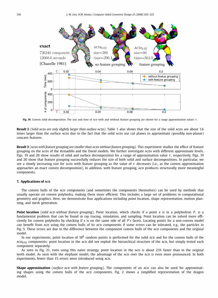
518 J.-M. Lien, N.M. Amato / Computer Aided Geometric Design 25 (2008) 503–522
Fig. 19. Convex solid decomposition. The size and time of acd with and without feature grouping are shown for a range approximation values τ .
Result 2 (Solid acds are only slightly larger than surface acds). Table 1 also shows that the size of the solid acds are about 1.6times larger than the surface acds due to the fact that the solid acds use cut planes to approximate (possibly non-planar)concave features.
Result 3 (acds with feature grouping are smaller than acds without feature grouping). This experiment studies the effect of featuregrouping on the acds of the Armadillo and the David models. We further investigate acds with different approximate levels.Figs. 19 and 20 show results of solid and surface decomposition for a range of approximation value τ , respectively. Figs. 19and 20 show that feature grouping successfully reduces the size of both solid and surface decompositions. In particular, wesee a slowly increasing size for acds with feature grouping as the value of τ decreases (i.e., as the convex approximationapproaches an exact convex decomposition). In addition, with feature grouping, acd produces structurally more meaningfulcomponents.
7. Applications of ACD
The convex hulls of the acd components (and sometimes the components themselves) can be used by methods thatusually operate on convex polyhedra, making them more efficient. This includes a large set of problems in computationalgeometry and graphics. Here, we demonstrate four applications including point location, shape representation, motion plan-ning, and mesh generation.
Point location (solid acd without feature grouping). Point location, which checks if a point x is in a polyhedron P , is afundamental problem that can be found in ray tracing, simulation, and sampling. Point location can be solved more effi-ciently for convex polyhedra by checking if x is on the same side of all P ’s facets. Locating points for a non-convex modelcan benefit from acd using the convex hulls of its acd components if some errors can be tolerated, e.g., the particles inFig. 5. These errors are due to the difference between the component convex hulls of the acd components and the originalmodel.
In our experiments, point location of 108 random points is performed for the solid ecd and for the convex hulls of theacd0.02 components; point location in the acd did not exploit the hierarchical structure of the acd, but simply tested eachcomponent separately.
As seen in Fig. 21, even using this naive strategy, point location in the acd is about 23% faster than in the originalteeth model. As seen with the elephant model, the advantage of the acd over the ecd is even more pronounced. In bothexperiments, fewer than 1% errors were introduced using acd.
Shape approximation (surface acd with feature grouping). The components of an acd can also be used for approximat-ing shapes using the convex hulls of the acd components. Fig. 2 shows a simplified representation of the dragonmodel.
J.-M. Lien, N.M. Amato / Computer Aided Geometric Design 25 (2008) 503–522 519
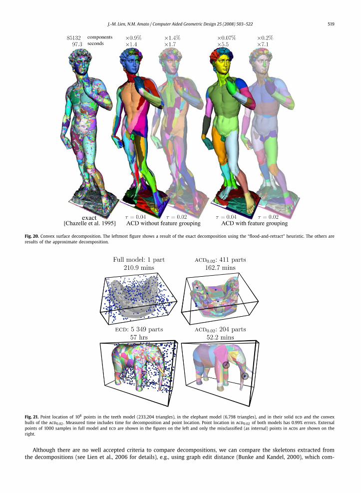
Fig. 20. Convex surface decomposition. The leftmost figure shows a result of the exact decomposition using the “flood-and-retract” heuristic. The others areresults of the approximate decomposition.
Fig. 21. Point location of 108 points in the teeth model (233,204 triangles), in the elephant model (6,798 triangles), and in their solid ecd and the convexhulls of the acd0.02. Measured time includes time for decomposition and point location. Point location in acd0.02 of both models has 0.99% errors. Externalpoints of 1000 samples in full model and ecd are shown in the figures on the left and only the misclassified (as internal) points in acds are shown on theright.
Although there are no well accepted criteria to compare decompositions, we can compare the skeletons extracted fromthe decompositions (see Lien et al., 2006 for details), e.g., using graph edit distance (Bunke and Kandel, 2000), which com-
520 J.-M. Lien, N.M. Amato / Computer Aided Geometric Design 25 (2008) 503–522
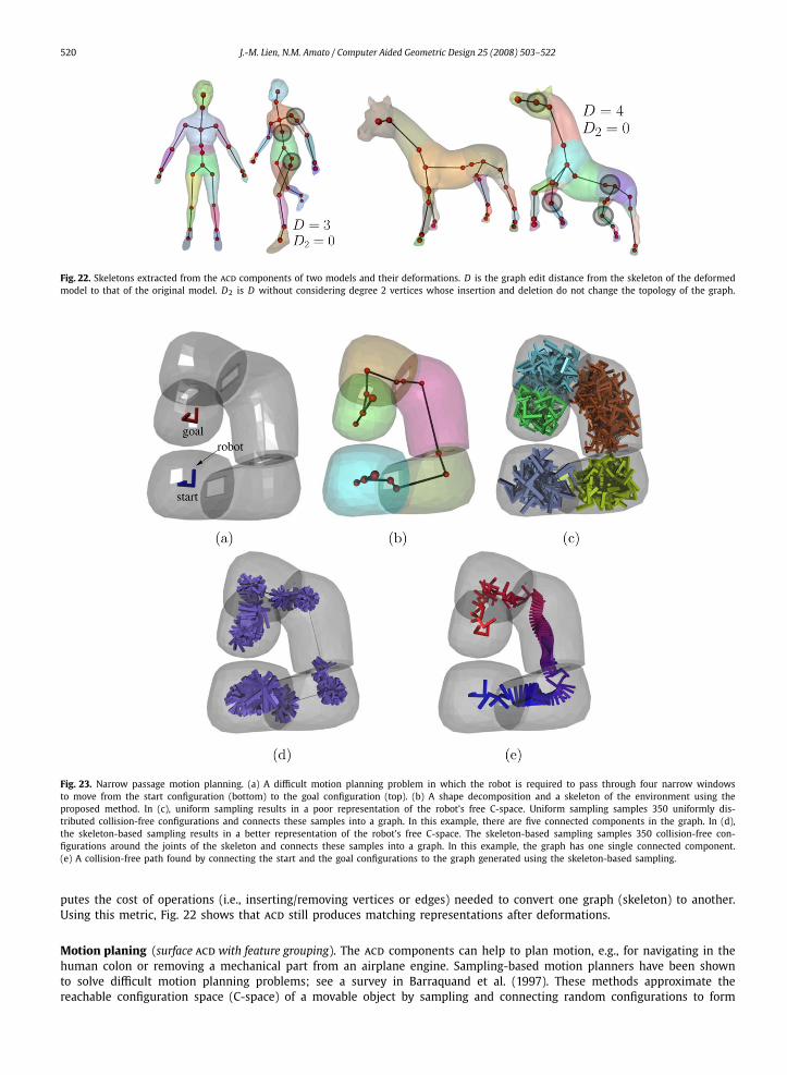
Fig. 22. Skeletons extracted from the acd components of two models and their deformations. D is the graph edit distance from the skeleton of the deformedmodel to that of the original model. D2 is D without considering degree 2 vertices whose insertion and deletion do not change the topology of the graph.
Fig. 23. Narrow passage motion planning. (a) A difficult motion planning problem in which the robot is required to pass through four narrow windowsto move from the start configuration (bottom) to the goal configuration (top). (b) A shape decomposition and a skeleton of the environment using theproposed method. In (c), uniform sampling results in a poor representation of the robot’s free C-space. Uniform sampling samples 350 uniformly dis-tributed collision-free configurations and connects these samples into a graph. In this example, there are five connected components in the graph. In (d),the skeleton-based sampling results in a better representation of the robot’s free C-space. The skeleton-based sampling samples 350 collision-free con-figurations around the joints of the skeleton and connects these samples into a graph. In this example, the graph has one single connected component.(e) A collision-free path found by connecting the start and the goal configurations to the graph generated using the skeleton-based sampling.
putes the cost of operations (i.e., inserting/removing vertices or edges) needed to convert one graph (skeleton) to another.Using this metric, Fig. 22 shows that acd still produces matching representations after deformations.
Motion planing (surface acd with feature grouping). The acd components can help to plan motion, e.g., for navigating in thehuman colon or removing a mechanical part from an airplane engine. Sampling-based motion planners have been shownto solve difficult motion planning problems; see a survey in Barraquand et al. (1997). These methods approximate thereachable configuration space (C-space) of a movable object by sampling and connecting random configurations to form
J.-M. Lien, N.M. Amato / Computer Aided Geometric Design 25 (2008) 503–522 521
a graph (or a tree). However, they also have several technical issues limiting their success on some important types ofproblems, such as the difficulty of finding paths that are required to pass through narrow passages.
acd can address the so called “narrow passage” problem for some problems by sampling with a bias toward cuts betweenthe acd components of a workspace (for rigid or articulated robots). Fig. 3 illustrates the advantage of this sampling strategyover uniform sampling (Kavraki et al., 1996). Advantages of the acd-based sampling are that more samples are placed inthe narrower (difficult) regions and also the connections between the samples can be made more easily due to the nearlyconvex components.
Moreover, the acd components provide a mechanism for extracting skeletons (Lien et al., 2006), which are natural struc-ture for planning motion. Fig. 23 shows that the graph constructed using skeleton can better represent the free C-spacethan using the uniform sampling (Kavraki et al., 1996) with the same number of samples.
Mesh generation (solid acd with feature grouping). The acd components can be used to generate tetrahedral meshes fromthe convex hulls of the acd components using Delaunay triangulation. The convex hulls may further simplified, e.g., usingtriboxes (Crosnier and Rossignac, 1999), to generate even coarser meshes. These meshes can later be used for, e.g., surfacedeformation. An illustration of this application is shown in Fig. 4.
8. Discussion and future work
We have presented a framework for decomposing a given polyhedron of arbitrary genus into nearly convex components.This provides a mechanism by which significant features are removed and insignificant features can be allowed to remainin the final approximate convex decomposition (acd). We have also demonstrated that the acd framework is flexible—bysimply changing the decomposition criterion from concavity to convexity, the acd can be used as a shape descriptor of theinput model.
Despite our promising results, our current implementation has some limitations which we plan to address in future work,some of which can be solved without too much difficulty. For example, some uncommon types of open surfaces with non-zero genus, whose vertices on the convex hull are all convex, cannot be handled correctly by the proposed method. Also,splitting non-linearly separable features using a best fit cut plane can still generate a visually unpleasant decomposition.One possible way to address this problem is to use curved cut surfaces.
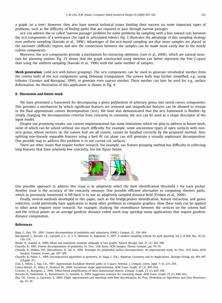
There are other issues that require further research. For example, our feature grouping method has difficulty in collectinglong features that have relatively low concavity. See the figure below.
One possible approach to address this issue is to adaptively select the knot identification threshold δ for each pocket.Another issue is the accuracy of the concavity measure. One possible efficient alternative to computing shortest paths,which as previously mentioned is NP-hard, is to use an adaptively sampled distance field (Frisken et al., 2000).
Finally, several methods developed in this paper, such as the bridge/pocket identification, feature extraction, and genusreduction, could potentially have application to many other problems in computer graphics. How these tools can be appliedto other areas requires more research. For example, studying the resemblance between the vertices on the convex hulland the critical points on an average geodesic distance coded mesh may speedup many applications that require geodesicdistance computation.
References
Bajaj, C., Dey, T.K., 1992. Convex decomposition of polyhedra and robustness. SIAM J. Comput. 21, 339–364.Barraquand, J., Kavraki, L.E., Latombe, J.-C., Li, T.-Y., Motwani, R., Raghavan, P., 1997. A random sampling scheme for path planning. Int. J. of Rob. Res. 16 (6),
759–774.Bunke, H., Kandel, A., 2000. Mean and maximum common subgraph of two graphs. Pattern Recogn. Lett. 21 (2), 163–168.Chazelle, B., 1981. Convex decompositions of polyhedra. In: Proc. 13th Annu. ACM Sympos. Theory Comput., pp. 70–79.Chazelle, B., Dobkin, D.P., Shouraboura, N., Tal, A., 1995. Strategies for polyhedral surface decomposition: An experimental study. In: Proc. 11th Annu. ACM
Sympos. Comput. Geom., pp. 297–305.Chazelle, B., Palios, L., 1994. Decomposition algorithms in geometry. In: Bajaj, C. (Ed.), Algebraic Geometry and its Applications. Springer-Verlag, pp. 419–447
(Chapter 27).Choi, J., Sellen, J., Yap, C.K., 1997. Approximate Euclidean shortest paths in 3-space. Internat. J. Comput. Geom. Appl. 7 (4), 271–295.Cohen-Steiner, D., Alliez, P., Desbrun, M., 2004. Variational shape approximation. ACM Trans. Graph. 23 (3), 905–914.Crosnier, A., Rossignac, J., 1999. Tribox-based simplification of three-dimensional objects. Comput. Graph. 23 (3), 429–438.DeCarlo, D., Finkelstein, A., Rusinkiewicz, S., Santella, A., 2003. Suggestive contours for conveying shape. ACM Trans. Graph. 22 (3), 848–855.Dey, T.K., Giesen, J., Goswami, S., 2003. Shape segmentation and matching with flow discretization. In: Proc. Workshop on Algorithms and Data Structures,
pp. 25–36.
522 J.-M. Lien, N.M. Amato / Computer Aided Geometric Design 25 (2008) 503–522
Erickson, J., Har-Peled, S., 2002. Optimally cutting a surface into a disk. In: Proceedings of the Eighteenth Annual Symposium on Computational Geometry.ACM Press, pp. 244–253.
Frisken, S.F., Perry, R.N., Rockwood, A.P., Jones, T.R., 2000. Adaptively sampled distance fields: a general representation of shape for computer graphics. In:Proc. ACM SIGGRAPH, pp. 249–254.
Funkhouser, T., Kazhdan, M., Shilane, P., Min, P., Kiefer, W., Tal, A., Rusinkiewicz, S., Dobkin, D., 2004. Modeling by example. ACM Trans. Graph. 23 (3),652–663.
Goswami, S., Dey, T.K., Bajaj, C.L., 2006. Identifying flat and tubular regions of a shape by unstable manifolds. In: SPM ’06: Proceedings of the 2006 ACMSymposium on Solid and Physical Modeling. ACM Press, New York, NY, USA, pp. 27–37.
Hershberger, J., Snoeyink, J., 1992. Speeding up the Douglas–Peucker line simplification algorithm. In: Proc. 5th Internat. Sympos. Spatial Data Handling, pp.134–143.
Hubeli, A., Gross, M., 2001. Multiresolution feature extraction for unstructured meshes. In: Proceedings of the conference on Visualization ’01, pp. 287–294.Joe, B., 1994. Tetrahedral mesh generation in polyhedral regions based on convex polyhedron decompositions. Internat. J. Numer. Methods Engrg. 37, 693–
713.Katz, S., Tal, A., 2003. Hierarchical mesh decomposition using fuzzy clustering and cuts. ACM Trans. Graph. 22 (3), 954–961.Kavraki, L.E., Svestka, P., Latombe, J.C., Overmars, M.H., 1996. Probabilistic roadmaps for path planning in high-dimensional configuration spaces. IEEE Trans.
Robot. Automat. 12 (4), 566–580.Keil, J.M., 2000. Polygon decomposition. In: Sack, J.-R., Urrutia, J. (Eds.), Handbook of Computational Geometry. Elsevier Science Publishers B.V. North-
Holland, Amsterdam, pp. 491–518.Kent, J.R., Carlson, W.E., Parent, R.E., 1992. Shape transformation for polyhedral objects. SIGGRAPH Comput. Graph. 26 (2), 47–54.Khodakovsky, A., Litke, N., Schröder, P., 2003. Globally smooth parameterizations with low distortion. ACM Trans. Graph. 22 (3), 350–357.Lai, Y.-K., Zhou, Q.-Y., Hu, S.-M., Martin, R.R., 2006. Feature sensitive mesh segmentation. In: SPM ’06: Proceedings of the 2006 ACM Symposium on Solid
and Physical Modeling. ACM Press, New York, NY, USA, pp. 17–25.Lee, Y., Lee, S., Shamir, A., Cohen-Or, D., Seidel, H.-P., 2005. Mesh scissoring with minima rule and part salience. Comput. Aided Geom. Des. 22 (5), 444–465.Lévy, B., Petitjean, S., Ray, N., Maillot, J., 2002. Least squares conformal maps for automatic texture atlas generation. In: Proceedings of the 29th Annual
Conference on Computer Graphics and Interactive Techniques, pp. 362–371.Li, X., Toon, T.W., Huang, Z., 2001. Decomposing polygon meshes for interactive applications. In: Proceedings of the 2001 Symposium on Interactive 3D
Graphics, pp. 35–42.Lien, J.-M., Amato, N.M., 2004. Approximate convex decomposition of polygons. In: Proc. 20th Annual ACM Symp. Computat. Geom. (SoCG), pp. 17–26.Lien, J.-M., Keyser, J., Amato, N.M., 2006. Simultaneous shape decomposition and skeletonization. In: SPM ’06: Proceedings of the 2006 ACM Symposium on
Solid and Physical Modeling. ACM Press, New York, NY, USA, pp. 219–228.Liu, S., Martin, R.R., Langbein, F.C., Rosin, P.L., 2006. Segmenting reliefs on triangle meshes. In: SPM ’06: Proceedings of the 2006 ACM Symposium on Solid
and Physical Modeling. ACM Press, New York, NY, USA, pp. 7–16.Mangan, A.P., Whitaker, R.T., 1999. Partitioning 3d surface meshes using watershed segmentation. IEEE Trans. Vis. Comput. Graph. 5 (4), 308–321.Ohtake, Y., Belyaev, A., Seidel, H.-P., 2004. Ridge-valley lines on meshes via implicit surface fitting. ACM Trans. Graph. 23 (3), 609–612.Pauly, M., Keiser, R., Gross, M., 2003. Multi-scale feature extraction on point-sampled surfaces. In: Proceedings of the Eurographics/ACM SIGGRAPH Sympo-
sium on Geometry Processing, pp. 281–289.Praun, E., Hoppe, H., 2003. Spherical parametrization and remeshing. ACM Trans. Graph. 22 (3), 340–349.Rom, H., Medioni, G., 1994. Part decomposition and description of 3d shapes. In: Proc. International Conference of Pattern Recognition, pp. 629–632.Rusinkiewicz, S., 2004. Estimating curvatures and their derivatives on triangle meshes. In: 3D Data Processing, Visualization, and Transmission, 2nd Inter-
national Symposium on (3DPVT’04), pp. 486–493.Shapiro, A., Tal, A., 1998. Polyhedron realization for shape transformation. Vis. Comput. 14 (8/9), 429–444.Sharir, M., Schorr, A., 1986. On shortest paths in polyhedral spaces. SIAM J. Comput. 15, 193–215.Sklansky, J., 1972. Measuring concavity on rectangular mosaic. IEEE Trans. Comput. C-21, 1355–1364.White, E.R., 1985. Assessment of line-generalization algorithms using characteristic points. Amer. Cartographer 12 (1), 17–27.Wood, Z., Hoppe, H., Desbrun, M., Schröder, P., 2004. Removing excess topology from isosurfaces. ACM Trans. Graph. 23 (2), 190–208.Wu, K., Levine, M.D., 1994. Recovering parametric geons from multiview range data. In: Proc. International Conference of Pattern Recognition, pp. 159–166.Wu, K., Levine, M.D., 1997. 3d part segmentation using simulated electrical charge distributions. IEEE Trans. Pattern Anal. Machine Intell. 19 (11), 1223–1235.Yamauchi, H., Lee, S., Lee, Y., Ohtake, Y., Belyaev, A., Seidel, H.-P., 2005. Feature sensitive mesh segmentation with mean shift. In: SMI ’05: Proceedings of
the International Conference on Shape Modeling and Applications 2005 (SMI’ 05). IEEE Computer Society, Washington, DC, USA, pp. 238–245.Yoshizawa, S., Belyaev, A., Seidel, H.-P., 2005. Fast and robust detection of crest lines on meshes. In: SPM ’05: Proceedings of the 2005 ACM Symposium on
Solid and Physical Modeling. ACM Press, New York, NY, USA, pp. 227–232.Zhang, E., Mischaikow, K., Turk, G., 2005. Feature-based surface parameterization and texture mapping. ACM Trans. Graph. 24 (1), 1–27.Zunic, J., Rosin, P.L., 2002. A convexity measurement for polygons. In: British Machine Vision Conference, pp. 173–182.