Embed Size (px)
Citation preview
RESEARCH ARTICLE
Concerning the matching of magnetic
susceptibility differences for the
compensation of background gradients in
anisotropic diffusion fibre phantoms
Ezequiel Farrher1☯*, Johannes Lindemeyer1☯, Farida Grinberg1,2, Ana-Maria Oros-
Peusquens1, N. Jon Shah1,2,3,4,5
1 Institute of Neuroscience and Medicine – 4, Forschungszentrum Julich GmbH, Julich, Germany,
2 Department of Neurology, Faculty of Medicine, RWTH Aachen University, Aachen, Germany, 3 JARA –
BRAIN – Translational Medicine, RWTH Aachen University, Aachen, Germany, 4 Institute of Neuroscience
and Medicine – 11, Forschungszentrum Julich GmbH, Julich, Germany, 5 Department of Electrical and
Computer Systems Engineering, and Monash Biomedical Imaging, School of Psychological Sciences,
Monash University, Melbourne, Victoria, Australia
☯ These authors contributed equally to this work.
Abstract
Artificial, anisotropic fibre phantoms are nowadays increasingly used in the field of diffusion-
weighted MRI. Such phantoms represent useful tools for, among others, the calibration of
pulse sequences and validation of diffusion models since they can mimic well-known struc-
tural features of brain tissue on the one hand, but exhibit a reduced complexity, on the other.
Among all materials, polyethylene fibres have been widely used due to their excellent prop-
erties regarding the restriction of water diffusion and surface relaxation properties. Yet the
magnetic susceptibility of polyethylene can be distinctly lower than that of distilled water.
This difference produces strong microscopic, background field gradients in the vicinity of
fibre bundles which are not parallel to the static magnetic field. This, in turn, modulates the
MRI signal behaviour. In the present work we investigate an approach to reduce the suscep-
tibility-induced background gradients via reducing the heterogeneity in the internal magnetic
susceptibility. An aqueous solution of magnesium chloride hexahydrate (MgCl2�6H2O) is
used for this purpose. Its performance is demonstrated in dedicated anisotropic fibre phan-
toms with different geometrical configurations.
Introduction
Diffusion phantoms are highly demanded devices for a broad set of applications in diffusion-
weighted (DW) MRI. These applications include the design and calibration of DW MRI
experiments [1–5], validation and optimisation of high angular resolution diffusion imaging
(HARDI) methods [6–10], tractography algorithms [11–13], validation of diffusion models
[14,15] and results from multi-centre studies [16,17]. Artificial, anisotropic diffusion
PLOS ONE | https://doi.org/10.1371/journal.pone.0176192 May 3, 2017 1 / 20
a1111111111
a1111111111
a1111111111
a1111111111
a1111111111
OPENACCESS
Citation: Farrher E, Lindemeyer J, Grinberg F,
Oros-Peusquens A-M, Shah NJ (2017) Concerning
the matching of magnetic susceptibility differences
for the compensation of background gradients in
anisotropic diffusion fibre phantoms. PLoS ONE 12
(5): e0176192. https://doi.org/10.1371/journal.
pone.0176192
Editor: Quan Jiang, Henry Ford Health System,
UNITED STATES
Received: January 27, 2017
Accepted: April 6, 2017
Published: May 3, 2017
Copyright: © 2017 Farrher et al. This is an open
access article distributed under the terms of the
Creative Commons Attribution License, which
permits unrestricted use, distribution, and
reproduction in any medium, provided the original
author and source are credited.
Data Availability Statement: All relevant data are
within the paper and its Supporting Information
files.
Funding: The authors received no specific funding
for this work.
Competing interests: The authors have declared
that no competing interests exist.
phantoms found in the literature are made of a large variety of materials, e.g., rayon [6,18],
hemp [18], polyester [1,5], acrylic fibres [13], glass capillaries [19], plastic capillaries [3,9], hol-
low fibres produced by co-electrospinning [2,12] and polyamide fibres [4,10]. One of the most
frequently used materials is Dyneema1 [14,15,18,20,21] (Dyneema1 SK75 dtex1760, DSM,
Geleen, The Netherlands). These rod-like, hydrophobic, polyethylene fibres have several
advantages concerning physical properties compared to other synthetic materials such as
nylon and fibre glass, particularly its lower surface relaxivity that results in overall longer
relaxation times [20]. This enables diffusion measurements to be performed with higher sig-
nal-to-noise ratio (SNR) or longer echo times, which is especially important in the case of
strong diffusion weightings and time-dependent studies. Mechanical flexibility is also an
advantage when compared to, for instance, rigid capillaries, given that this flexibility facilitates
manufacturing of phantoms with a wide range of geometrical configurations. Another advan-
tage of Dyneema1 fibres is that they are available with radii below 10 microns, which makes
them well-suited for producing phantoms with sufficiently dense diffusion barriers, compara-
ble to that of cellular structures.
Magnetostatic theory predicts that two media of different magnetic susceptibility, χ, placed
in an external magnetic field introduce distortions to the field distribution in the vicinity of
their interface [22]. These distortions, i.e., magnetic field gradients, depend on the difference
in magnetic susceptibility, Δχ = χ2 - χ1, as well as on the geometric configuration of the media
(curvature radii, interface orientation relative to the magnetic field, etc.). Thus, microscopic,
susceptibility-induced magnetic field gradients (further on referred to as background gradi-
ents) are ubiquitous in NMR and MRI experiments involving magnetically heterogeneous
media such as, among others, porous materials [23–25] and biological tissues [26–29]. In par-
ticular, background gradients appear as a common feature in anisotropic diffusion phantoms
where the magnetic susceptibility of the diffusing liquid is a priori different from that of the
diffusion-restricting material [4,20,21,30].
As initially demonstrated by Stejskal and Tanner [31], the DW NMR signal in an infinite
medium as measured using conventional pulsed gradient spin-echo (PGSE) sequences in the
presence of constant background gradients, is influenced by three distinct terms: i) a term
dependent on the externally applied field gradient g, ii) a term purely dependent on the
background gradients g0, and iii) an interference, cross-term resulting from the interaction
between the background and the externally applied gradients. In SE experiments without
externally applied field gradients, background gradients act, in the interplay with the diffusion
process, as an extra mechanism reducing the measured transverse relaxation time, T2 [24].
This feature has been successfully used to provide biomarkers of trabecular bone density
[27,32,33] or muscle microstructure [34], for example. Recently, computer simulations were
used [35] to study the orientation-dependence of T2 due to background gradients in an array
of cylinders under different configurations of Δχ, cylinder packing density and order.
In conventional PGSE, experiments are carried out by measuring the echo attenuation for
several strengths of the diffusion-sensitising field gradient g, while keeping the sequence tim-
ing constant [36]. As a consequence, the signal attenuation due to g0 becomes merely a multi-
plicative factor. Special care must be taken though when the strength of g0 is so large that the
signal-to-noise ratio (SNR) becomes critically low for a given echo-time. It has been shown
that low values of the SNR in the magnitude signal can lead to a strong underestimation of the
apparent diffusion coefficient [37]. On the other hand, the cross-term can lead to more com-
plex implications. It is a priori spatially dependent, and therefore it may be cancelled in some
regions whereas it may be greatly enhanced in others, even for small g0 strengths. The effect of
the cross-term has previously been measured and empirically modelled by Zhong et al. [38,39]
in artificial samples, post mortem and in rat tissue in vivo. Their results demonstrate an
Matching magnetic susceptibility in diffusion MRI phantoms
PLOS ONE | https://doi.org/10.1371/journal.pone.0176192 May 3, 2017 2 / 20
increase in the echo amplitude for increasing g0 strengths. This was interpreted as an effect of
the regions where g was compensated by g0. The same empirical model was later used by Clark
et al. [28] for the analysis of in vivo human brain data, showing similar results. In this context,
the same increase in the echo amplitude due to background gradients introduced by the
microvessels in the human brain was predicted by Kiselev [40], employing a more realistic
model for brain microvasculature.
While background gradients can be exploited to obtain additional structural information
on tissue microstructure and orientation [41–45], they can lead to misinterpretation of the
results, if they are not properly taken into account in the context of most DW MRI measure-
ments [28,38–40]. Therefore, in many DW MRI experiments, background gradients represent
unwanted entities which need to be cancelled. A reduction of the effect of background gradi-
ents has been achieved via the design of advanced pulse sequences, as an alternative to the con-
ventional Stejskal-Tanner PGSE sequence [31]. Some of the sequences attempt to reduce the
effect of the g0 term [46,47], whereas others are meant to suppress the effect of the cross-term
[46,48]. Nevertheless, a strong underlying assumption in these methods is that the background
gradients change slowly throughout space, meaning that each diffusing molecule experiences
the same constant background gradient during the observation time. Ref. [46] provides a com-
prehensive review on this topic.
A different approach for the suppression of background gradients is susceptibility match-
ing. Its aim is to reduce, or ideally entirely eliminate, the difference in magnetic susceptibilities
within the sample. This approach has been previously used in NMR spectroscopy studies [49]
to reduce the line broadening in NMR spectra. More recently susceptibility matching was car-
ried out in a polyamide fibre phantom. In their work, Laun et al. [4] used a solution of 83
grams of sodium chloride (NaCl) per kilogram of distilled water, in order to match the suscep-
tibility of the solution to that of the polyamide fibres, which is 0.37 ppm more diamagnetic
than distilled water.
The aim of this work is to design a strategy to suppress unwanted background gradients by
matching the susceptibility of the liquid to that of the fibre material. In order to achieve this,
the effects of background gradients on diffusion metrics in anisotropic phantoms constructed
with Dyneema1 fibres and different fibre configurations are assessed. We investigate the influ-
ence of background gradients on diffusion tensor imaging (DTI) invariant metrics, as well as
on two methods for the analysis of HARDI data, namely constrained spherical deconvolution
(CSD) [50] and q-ball imaging (QBI) [51]. Three types of dedicated phantoms were used for
this purpose: i) bulk phantoms, i.e., test vials containing the solution of interest embedded in a
cylindrical phantom; ii) parallel-fibre phantoms, i.e., showing single-modal diffusion profiles;
iii) a phantom with two fibre populations crossing at the right angle, i.e., showing multi-modal
diffusion profiles.
Theory
The PGSE signal attenuation for an infinite, homogeneous and anisotropic medium with uni-
form background gradients g0 = g0n0, in the presence of a diffusion sensitising, pulsed field
gradient g = gn, is given by [24,36]
Sðb;nÞ ¼ S0exp � b � nTDn|fflfflfflfflffl{zfflfflfflfflffl}
external
þ bc � nTDn0|fflfflfflfflfflfflffl{zfflfflfflfflfflfflffl}
cross term
0
@
1
A
2
4
3
5; ð1Þ
where S0 is the DW signal in the absence of diffusion weighting, D is the symmetric, positive-
definite diffusion tensor, and n and n0 are the unit vectors along the diffusion sensitising and
Matching magnetic susceptibility in diffusion MRI phantoms
PLOS ONE | https://doi.org/10.1371/journal.pone.0176192 May 3, 2017 3 / 20
background gradients, respectively. The b-value due to the applied gradient is given by
b ¼ g2
ðTE
0
ðt
0
gðt0Þdt0� �2
dt, whereas the b-value related to the cross-term can be shown to be
bc ¼ 2g2
ðTE
0
ðt
0
gðt0Þdt0� � ðt
0
g0ðt0Þdt0
� �
dt, with g(t) and g0(t) denoting the gradients wave-
forms, TE the echo time and γ the gyromagnetic ratio. For the conventional Stejskal-Tanner
PGSE sequence b = γ2g2δ2(Δ − δ/3) and bc = γ2gg0δ(Δ − δ/3)[TE − (Δ − δ)/2], where δ and Δ are
the time duration and separation of the field gradient pulses, respectively [40]. Eq (1) corre-
sponds to the conventional case in which the DW signal is acquired for several strengths of
the field gradient while keeping the sequence timing constant. Thus, S0 includes a diffusion
weighting term that is purely dependent on the background gradients, which effectively acts as
an extra mechanism inducing transverse relaxation.
In the framework of DTI analysis, estimation of tensor elements is performed by regressing
Sðb;nÞ ¼ S0exp � ðbnTDappnÞ
h i; ð2Þ
to the measured DW signal. In Eq (2) the apparent diffusion tensor, Dapp, is introduced to
emphasize the possible bias in D arising as a consequence of neglecting the cross term and the
dependence on the pulse sequence and timing parameters employed. It is worth noticing that
the diffusion weighting term related to background gradients only will not significantly bias
the estimation, provided that the SNR is high enough. In case S0 is close to the noise floor,
special care must be taken in order to avoid bias in the tensor elements. Conventionally,
regression of Eq (2) to the experimental data is performed via a least-squares minimisation
approach. However, for low SNR experiments the maximum likelihood estimator is preferred
in order to ensure unbiased estimation [52].
System with cylindrical geometry
For a system of perfectly aligned cylinders, the background gradients only have components in
the radial direction, i.e., perpendicular to the axis of symmetry [40]. Therefore, the DW signals
acquired utilising gradient directions parallel (n||) and perpendicular (n?) to the axis of sym-
metry can be calculated using Eq (1), yielding
Sðb;njjÞ ¼ S0exp � bDjjh i
and
Sðb;n?Þ ¼ S0exp � ðbþ bcnT?n0ÞD?
� �;
ð3Þ
where D|| and D? denote the diffusivities in the direction parallel and perpendicular to the axis
of symmetry, respectively. While the estimation of D|| using Eq (2) would remain unbiased,
the dot product nT?n0 can take positive (parallel), negative (anti-parallel) or zero values. In
such systems, this term may also vary throughout space. More importantly, for densely packed
systems the gradient may be non-linear in the length-scale of the molecular root mean square
displacement. Hence, the estimation of D? via Eq (2) can potentially be biased.
Material and methods
Selection of the appropriate compound
Pure water is diamagnetic with a magnetic susceptibility of about χwater = -9.05ppm [53]. The
susceptibility values of typical compounds range from strong paramagnetism (positive values)
Matching magnetic susceptibility in diffusion MRI phantoms
PLOS ONE | https://doi.org/10.1371/journal.pone.0176192 May 3, 2017 4 / 20
to comparably small diamagnetism (negative values). In particular, materials soluble in water
with a magnetic susceptibility lower than that of water are rare. The susceptibility of the fibre
material Dyneema1 is approximately -10ppm [20], which is about 1ppm below water. Promis-
ing candidates for lowering the susceptibility value of aqueous solutions are salts since they are
typically good solutes in water and many of them are strongly diamagnetic. Unfortunately,
numerous salts also exhibit high electrical conductivity [54]. Hence compounds such as NaCl
or KCl are poor candidates for approaching high susceptibility differences due to their high
electrical conductivity and their consequently high radiofrequency absorption. Magnesium
Chloride (MgCl2) is diamagnetic with a susceptibility of χ = 4π � (ρ/M) � χm(cgs) = −14.6ppm,
χm(cgs) = -47.4cm3/mol [55], where ρ is the density and M represents the molar mass. It is also
highly soluble in water with up to 552 g/l at 20˚C [55] and its conductivity at a mass percentage
of 25% is roughly half that of e.g. NaCl [54]. The hydrated form, magnesium chloride hexahy-
drate (MgCl2�6H2O) can be easily mixed with water. Accurate values of the magnetic suscepti-
bility of different MgCl2�6H2O concentrations in distilled water are to our knowledge not
reported in literature.
Bulk experiments
All MRI experiments were carried out in a whole-body 3T Siemens MAGNETOM Trio scan-
ner (Siemens Medical Systems, Erlangen, Germany). The body coil was used for radiofre-
quency transmission and a 12-channel phased-array head coil was used for signal reception.
All experiments were performed at room temperature. The gradient system provided a maxi-
mal gradient strength of 40 mT/m.
A set of 9 solutions was prepared with increasing MgCl2�6H2O concentrations, cv (v = 0,. . .,8),
in distilled water in order to assess bulk NMR properties (Table 1). Test vials were filled with
these solutions and embedded, one at a time, into a cylindrical polyethylene terephthalate (PET)
plastic phantom (10 cm diameter, 14 cm height) filled with distilled water (Fig 1a).
Magnetic susceptibility is assessed via the field distortions generated by the cylindrical tube
in the surrounding water as in quantitative susceptibility imaging (QSM, [56,57]). The stron-
gest distortions can be achieved with the cylinder orientation perpendicular to the static mag-
netic field [58]. The field distribution inside the phantom is estimated by linear regression on
the phase data acquired with a multiple-echo, gradient-echo (GRE) sequence at 1mm isotropic
resolution; matrix-size, 128×128×160; flip-angle, 14˚; TE = 3ms (8 echoes, ΔTE = 4ms; band-
width, BW = 501 Hz/pixel); repetition time, TR = 60ms; using monopolar readout. Automated
threshold- and morphology-based segmentation is applied to the signal magnitude in order
to generate masks for the vial content, mv, and the water volume, mw. An evaluation area
surrounding the vial, me, is defined by expanding the vial mask. Our in-house software,
MUBAFIRE [59], is used to correct for field distortions originating from sources outside of the
phantom. The susceptibility distribution χv inside the vial is assumed to be constant as the liq-
uid is homogeneous. Furthermore, setting χ to 0 within the water mask defines χwater as the
reference offset. The difference between the measured field and the one generated by dipole
convolution [60] of χv within a cylindrical water mask, me, around the test vial is evaluated
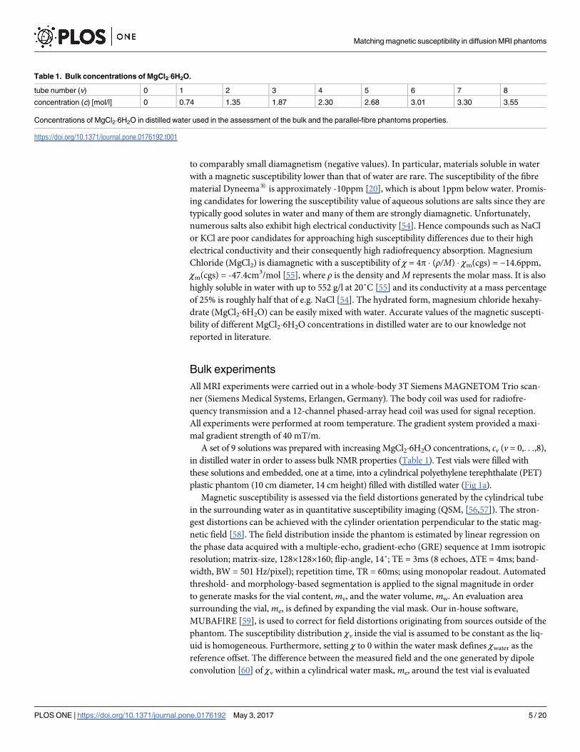
Table 1. Bulk concentrations of MgCl2�6H2O.
tube number (v) 0 1 2 3 4 5 6 7 8
concentration (c) [mol/l] 0 0.74 1.35 1.87 2.30 2.68 3.01 3.30 3.55
Concentrations of MgCl2�6H2O in distilled water used in the assessment of the bulk and the parallel-fibre phantoms properties.
https://doi.org/10.1371/journal.pone.0176192.t001
Matching magnetic susceptibility in diffusion MRI phantoms
PLOS ONE | https://doi.org/10.1371/journal.pone.0176192 May 3, 2017 5 / 20
(Fig 2) and minimised for χv:
minwvkme � ðBmeas � B0 � ½wvmv d�Þk2; ð4Þ
where d is the appropriate dipole kernel [61]. The internal stray field of the vial can bias the
background field correction. In order to compensate for this effect, background correction
and susceptibility estimation are iterated three times. In each iteration, the estimated vial field
of the previous iteration is subtracted during background correction. The whole procedure is
illustrated in Fig 2. The accuracy of the susceptibility estimate is indicated by the relative differ-
ence between background-corrected field and the field generated by the determined suscepti-
bility χv, evaluated within me. Error values are defined as the mean-corrected field difference
divided by the mean-corrected measured field.
For the measurement of the bulk T1 relaxation times all vials were placed in the so-called
“revolver phantom”. Measurements were performed with the TAPIR sequence [62]. Protocol
parameters were: TR = 25 ms; flip-angle, 20˚, inversion-times, 20� TI� 4180 ms; BW = 320
Hz/pixel; voxel size, 1×1×4 mm3; matrix-size, 200×200×1. Data were processed using in-house
Matlab scripts (Matlab 2015a, The MathWorks, Natick, MA, USA).
The bulk T2 and proton density (PD) for all vials are estimated with the help of a 2D spin-
echo multi-contrast sequence provided by the manufacturer, using the following protocol
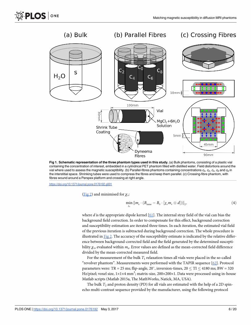
Fig 1. Schematic representation of the three phantom types used in this study. (a) Bulk phantoms, consisting of a plastic vial
containing the concentration of interest, embedded in a cylindrical PET phantom filled with distilled water. Field distortions around the
vial where used to assess the magnetic susceptibility. (b) Parallel-fibres phantoms containing concentrations c0, c2, c4, c6 and c8 in
the interstitial space. Shrinking tubes were used to compress the fibres and keep them parallel. (c) Crossing-fibre phantom, with
fibres wound around a Perspex platform and crossing at right angle.
https://doi.org/10.1371/journal.pone.0176192.g001
Matching magnetic susceptibility in diffusion MRI phantoms
PLOS ONE | https://doi.org/10.1371/journal.pone.0176192 May 3, 2017 6 / 20

parameters: 32 contrasts with an inter-echo time spacing of 50 ms; TR = 104 ms; number of
averages, AVGs = 3; BW = 781 Hz/pixel; voxel size, 2×2×10 mm3 and matrix-size, 96×128×1.
The echo attenuation, S(TE), is assumed to be monoexponential
SðTEÞ ¼ S0exp �TE
T2
� �
; ð5Þ
where S0 is the signal at TE = 0. S0 and T2 are estimated voxel-wise via non-linear least-squares
using the Nelder-Mead algorithm with in-house Matlab scripts. Finally the PD for each con-
centration cv is evaluated as PDv = S0,v/S0,0, with S0,v being the corresponding signal at TE = 0
[14,21].
Measurement of the bulk diffusion coefficient, D, for all concentrations cv, was carried
out using a 2D twice-refocused SE (TRSE) EPI sequence with bipolar diffusion weighting gra-
dients provided by the manufacturer [63]. Protocol parameters were: TR/TE = 8000/112 ms;
AVGs = 16; BW = 1628 Hz/pixel; voxel-size, 2×2×10 mm3; matrix-size, 96×128×1; 16 b-values,
[0:0.2:3.0] ms/μm2 along a single gradient direction; GRAPPA acceleration factor 2, with 24
reference lines. All DW MRI experiments in this work are performed such that different b-val-
ues are achieved by varying the gradient strength g while keeping the timing parameters δ and
Δ constant. Considering the isotropic diffusion of this case, S0 and D are estimated voxel-wise
via non-linear maximisation of the log-likelihood function as described in the section Maxi-mum likelihood estimation of diffusion parameters.
Parallel-fibre phantom
All fibre phantoms were constructed using Dyneema1 fibres (rod-like fibres with a radius of
approximately 8 μm) [14,20,21]. Five parallel-fibre phantoms were built using bundles of
Fig 2. Data processing workflow for the assessment of the bulk magnetic susceptibility values.
Starting from the top left, the raw phase is spatially unwrapped, the echoes are realigned and the field map is
estimated by linear regression; background fields are removed using MUBAFIRE and a reduced ROI for
evaluation is selected; setting a constant susceptibility value inside of the vial volume, the difference between
the hereby generated and the measured field distortion is minimised; the process is iterated three times in
order to take the estimated vial field into account in the background correction.
https://doi.org/10.1371/journal.pone.0176192.g002
Matching magnetic susceptibility in diffusion MRI phantoms
PLOS ONE | https://doi.org/10.1371/journal.pone.0176192 May 3, 2017 7 / 20
Dyneema1 fibres aligned in parallel. Each bundle was placed inside a shrinking tube approxi-
mately 5 centimetres wide [14,20] and afterwards heated to shrink it to a final diameter of
about 2.5 centimetres. The fibre density for each phantom was 0.64 ± 0.02. Each phantom was
then embedded in plastic vials that were filled with MgCl2�6H2O concentrations c0, c2, c4, c6
and c8 (Table 1), in such a way that the interstitial space between the fibres was filled via capil-
lary force. Finally, all vials were assembled in a cylindrical PET plastic container (10 cm diame-
ter, 14 cm height) filled with distilled water for the subsequent MRI experiments (Fig 1b).
Experiments were carried out for five different orientations of the fibre bundles with respect
to the static field B0 at θ = 0˚, 22.5˚, 45˚, 67.5˚ and 90˚. The TRSE sequence was used. Protocol
parameters were: TR/TE = 4200/82 ms; AVGs = 10; BW = 1563 Hz/pixel; voxel-size, 2×2×2
mm3; matrix-size, 80×128×36; 5 b-values, [0:0.25:1.0] ms/μm2 along 30 gradient directions;
GRAPPA acceleration factor 2, with 24 reference lines; phase-encoding direction right-to-left.
An extra non-DW volume with opposite phase-encoding direction was acquired for the cor-
rection of EPI distortions.
Eddy-current and EPI distortion correction is applied to all volumes with the help of the
EDDY tool available in FSL [64–66]. Subsequently, the diffusion weighting directions are
reoriented according to the transformation matrices obtained in the former step [67]. Spatial
smoothing with a Gaussian convolution kernel (full-width-half-maximum 2.3 mm) is applied
to the images. Given the anisotropic nature of diffusion in this case, S0 and the apparent diffu-
sion tensor Dapp are estimated as described in the section Maximum likelihood estimation ofdiffusion parameters.
Crossing-fibre phantom
The crossing-fibre phantom was built by tightly winding the fibres around a Perspex support
(Plexiglas1) in order to keep the geometrical shape (Fig 1c). Several layers of fibres were
stacked in perpendicularly alternating directions in such a way that the resulting thickness was
approximately 10 mm [21]. The fibre density for this phantom was 0.68 ± 0.02. The whole
setup was immersed in a PET plastic cylindrical container (10 cm diameter, 4 cm height). In
order to assess the effect of internal gradients, two different cases were considered:
1. Unmatched case. The phantom was first filled with distilled water and the whole set of MRI
experiments was carried out.
2. Matched case. The phantom was drained and refilled with the matching MgCl2�6H2O con-
centration (see section Results: c3 = 1.87 mol/l with χ3� -1.01 ppm), repeating the same
MRI experiments.
In both cases the phantom was placed in a vacuum chamber for four hours in order to
remove remaining air bubbles.
Experiments were carried out for three orientations of the phantom such that the angle, θ,
between one of the fibre populations and B0 was θ = 0˚, 22.5˚ and 45˚. Thus, the angle between
the remaining fibre population and B0 was 90˚–θ = 90˚, 67.5˚ and 45˚, respectively. Protocol
parameters were: TR/TE = 5000/113 ms; AVGs = 8; BW = 1563 Hz/pixel; voxel size, 2×2×2
mm3; matrix size, 88×128×14; GRAPPA acceleration factor 2, with 24 reference lines; phase-
encoding direction right-to-left. An extra non-DW volume with the opposite phase-encoding
direction was acquired for the correction of EPI distortions. The applied b-values were: b = 0,
1.0 ms/μm2 (unmatched) and b = 0, 2.0 ms/μm2 (matched) along 64 gradient directions. The
different b-values for the unmatched and the matched cases were chosen so as to maintain the
comparability of the products (bD)unmatched and (bD)matched. The non-DW signal, S0, and the
Matching magnetic susceptibility in diffusion MRI phantoms
PLOS ONE | https://doi.org/10.1371/journal.pone.0176192 May 3, 2017 8 / 20
apparent diffusion tensor Dapp are estimated voxel-wise as described in the section Maximumlikelihood estimation of diffusion parameters.
An evaluation of the performance of the CSD and QBI methods in assessing fibre direction-
ality is also carried out. The normalised fibre orientation distribution (FOD) defined in the
framework of CSD and the orientation density function (ODF) in the case of QBI are obtained
voxel-wise using the toolbox ExploreDTI [68]. Results are generated using maximum spheri-
cal-harmonic order lmax = 6. Fibre orientations are assessed via the local maxima of the FOD
and ODF, using a Newton optimisation algorithm [69]. A threshold equal to 10% of the maxi-
mum peak is used to reject spurious peaks. The deviation angle, Δα, between the predicted and
the underlying, mean fibre direction is evaluated as
Dap ¼1
N
XN
i¼1
cos� 1Mp �mp;i
jMpj
!�����
�����; ð6Þ
where p = 1, 2 denotes the peak number, N is the number of voxels in the ROI, mp,i is the
voxel-wise unit vector pointing in the pth fibre direction and Mp is a vector pointing along the
average pth fibre direction, Mp¼XN
j¼1mp;j.
Maximum likelihood estimation of diffusion parameters
The maximum likelihood estimator (ML) is used in order to avoid bias in the diffusion param-
eters due to the low SNR observed in some of the DW experiments described above [52]. The
ML estimator is written as:
arg maxβ½logpXðXjSðβÞ;sÞ�; ð7Þ
where S(β) is the signal model (Eq (2)), β is a vector containing all parameters of interest, X is
a vector containing the measured signals xi, px = ∏ip(xi|S(β), σ) denotes the joint probability
density function for xi, and p(xi|S(β), σ) is the Rice distribution with background noise param-
eter σ [52]. Here, the parameter σ is estimated following the method proposed by Aja-Fernan-
dez et al. [70]. For each case, maximisation of Eq (7) is performed using the Nelder-Mead
algorithm with in-house Matlab scripts.
Further evaluation of the DTI invariant scalar maps, namely axial (AD), representing D||,
radial (RD), representing D?, and mean (MD) apparent diffusivities as well as fractional
anisotropy (FA), is performed as described elsewhere [36]. Furthermore, a ROI analysis is car-
ried out for all metrics. The brackets hAi denote the average of a given parameter A over a
ROI, whereas the standard deviation is calculated as sA ¼
ffiffiffiffiffiffiffiffiffiffiffiffiffiffiffiffiffiffiffiffiffiffiffiffiffiffiffiffiffiffiffiffiffiffiffiffiffiffiffiffiffiffiffiffiffiffiffiffiffiffiffiffiffiXN
i¼1ðAi � hAiÞ
2=ðN � 1Þ
q
,
where N is the number of voxels in the ROI.
Results
Bulk experiments
Fig 3 illustrates the bulk magnetic susceptibility difference with respect to distilled water, χ (a),
the relative proton density PD (b), the relaxation times T1 and T2 (c), and the bulk diffusion
coefficient D (d), for the 9 concentrations of MgCl2�6H2O (Table 1). The susceptibility estima-
tion shows high precision with a relative field error of around 2%. Increasing the concentra-
tion of MgCl2�6H2O leads to a monotonous decrease of all parameters. In particular, for the
concentration c3 (1.87 mol/l) the magnetic susceptibility is χ3� -1.01 ppm, which practically
matches the susceptibility of the Dyneema fibres (Fig 3a) [20]. Concomitant with that change
Matching magnetic susceptibility in diffusion MRI phantoms
PLOS ONE | https://doi.org/10.1371/journal.pone.0176192 May 3, 2017 9 / 20
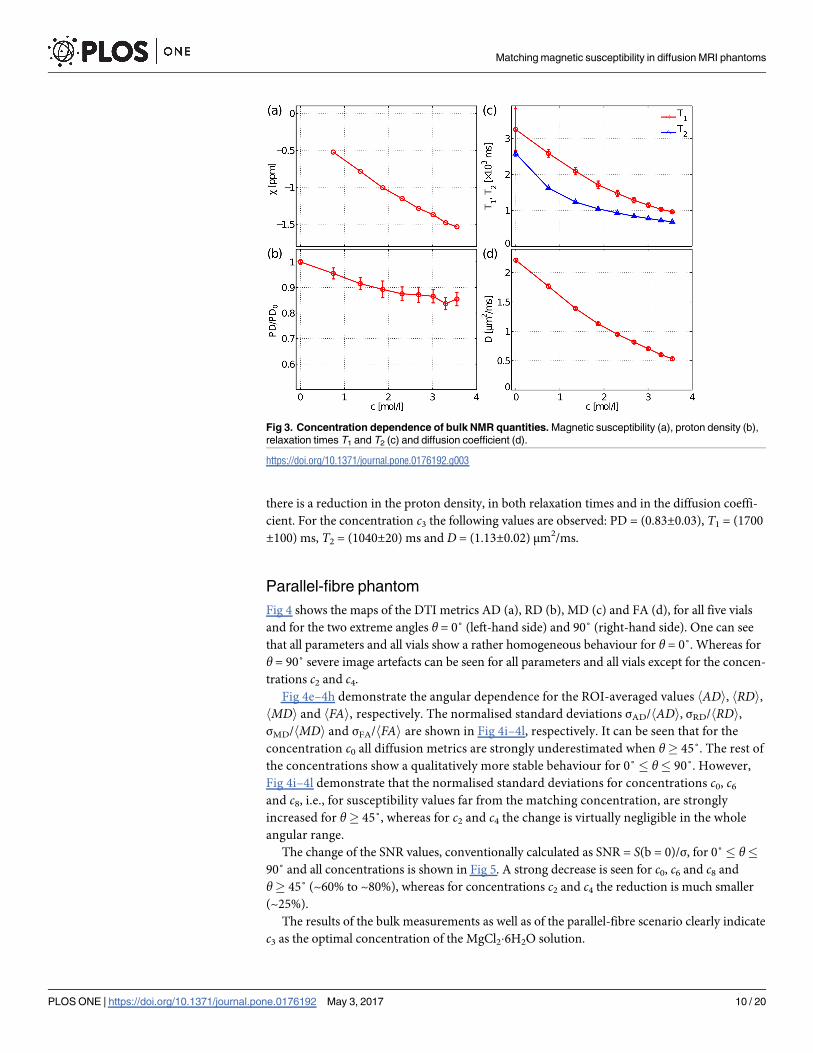
there is a reduction in the proton density, in both relaxation times and in the diffusion coeffi-
cient. For the concentration c3 the following values are observed: PD = (0.83±0.03), T1 = (1700
±100) ms, T2 = (1040±20) ms and D = (1.13±0.02) μm2/ms.
Parallel-fibre phantom
Fig 4 shows the maps of the DTI metrics AD (a), RD (b), MD (c) and FA (d), for all five vials
and for the two extreme angles θ = 0˚ (left-hand side) and 90˚ (right-hand side). One can see
that all parameters and all vials show a rather homogeneous behaviour for θ = 0˚. Whereas for
θ = 90˚ severe image artefacts can be seen for all parameters and all vials except for the concen-
trations c2 and c4.
Fig 4e–4h demonstrate the angular dependence for the ROI-averaged values hADi, hRDi,hMDi and hFAi, respectively. The normalised standard deviations σAD/hADi, σRD/hRDi,σMD/hMDi and σFA/hFAi are shown in Fig 4i–4l, respectively. It can be seen that for the
concentration c0 all diffusion metrics are strongly underestimated when θ� 45˚. The rest of
the concentrations show a qualitatively more stable behaviour for 0˚ � θ� 90˚. However,
Fig 4i–4l demonstrate that the normalised standard deviations for concentrations c0, c6
and c8, i.e., for susceptibility values far from the matching concentration, are strongly
increased for θ� 45˚, whereas for c2 and c4 the change is virtually negligible in the whole
angular range.
The change of the SNR values, conventionally calculated as SNR = S(b = 0)/σ, for 0˚� θ�90˚ and all concentrations is shown in Fig 5. A strong decrease is seen for c0, c6 and c8 and
θ� 45˚ (~60% to ~80%), whereas for concentrations c2 and c4 the reduction is much smaller
(~25%).
The results of the bulk measurements as well as of the parallel-fibre scenario clearly indicate
c3 as the optimal concentration of the MgCl2�6H2O solution.
Fig 3. Concentration dependence of bulk NMR quantities. Magnetic susceptibility (a), proton density (b),
relaxation times T1 and T2 (c) and diffusion coefficient (d).
https://doi.org/10.1371/journal.pone.0176192.g003
Matching magnetic susceptibility in diffusion MRI phantoms
PLOS ONE | https://doi.org/10.1371/journal.pone.0176192 May 3, 2017 10 / 20
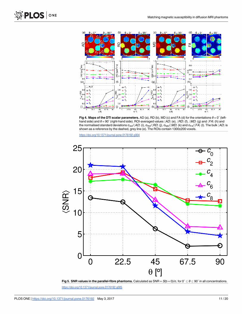
Fig 4. Maps of the DTI scalar parameters. AD (a), RD (b), MD (c) and FA (d) for the orientations θ = 0˚ (left-
hand side) and θ = 90˚ (right-hand side). ROI-averaged values hADi (e), hRDi (f), hMDi (g) and hFAi (h) and
the normalised standard deviations σAD/hADi (i), σRD/hRDi (j), σMD/hMDi (k) and σFA/hFAi (l). The bulk hADi is
shown as a reference by the dashed, grey line (e). The ROIs contain 1300±200 voxels.
https://doi.org/10.1371/journal.pone.0176192.g004
Fig 5. SNR values in the parallel-fibre phantoms. Calculated as SNR = S(b = 0)/σ, for 0˚� θ� 90˚ in all concentrations.
https://doi.org/10.1371/journal.pone.0176192.g005
Matching magnetic susceptibility in diffusion MRI phantoms
PLOS ONE | https://doi.org/10.1371/journal.pone.0176192 May 3, 2017 11 / 20
Crossing-fibre phantom
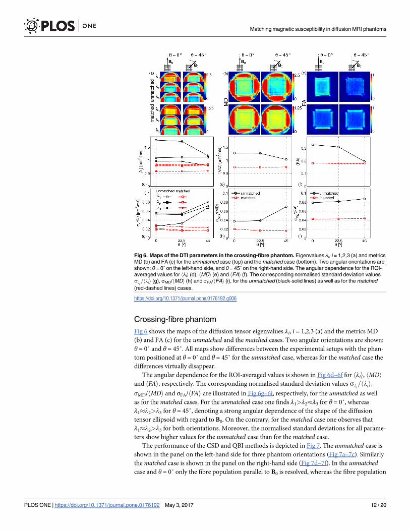
Fig 6 shows the maps of the diffusion tensor eigenvalues λi, i = 1,2,3 (a) and the metrics MD
(b) and FA (c) for the unmatched and the matched cases. Two angular orientations are shown:
θ = 0˚ and θ = 45˚. All maps show differences between the experimental setups with the phan-
tom positioned at θ = 0˚ and θ = 45˚ for the unmatched case, whereas for the matched case the
differences virtually disappear.
The angular dependence for the ROI-averaged values is shown in Fig 6d–6f for hλii, hMDiand hFAi, respectively. The corresponding normalised standard deviation values sli
=hlii,
σMD/hMDi and σFA/hFAi are illustrated in Fig 6g–6i, respectively, for the unmatched as well
as for the matched cases. For the unmatched case one finds λ1>λ2�λ3 for θ = 0˚, whereas
λ1�λ2>λ3 for θ = 45˚, denoting a strong angular dependence of the shape of the diffusion
tensor ellipsoid with regard to B0. On the contrary, for the matched case one observes that
λ1�λ2>λ3 for both orientations. Moreover, the normalised standard deviations for all parame-
ters show higher values for the unmatched case than for the matched case.
The performance of the CSD and QBI methods is depicted in Fig 7. The unmatched case is
shown in the panel on the left-hand side for three phantom orientations (Fig 7a–7c). Similarly
the matched case is shown in the panel on the right-hand side (Fig 7d–7f). In the unmatchedcase and θ = 0˚ only the fibre population parallel to B0 is resolved, whereas the fibre population
Fig 6. Maps of the DTI parameters in the crossing-fibre phantom. Eigenvalues λi, i = 1,2,3 (a) and metrics
MD (b) and FA (c) for the unmatched case (top) and the matched case (bottom). Two angular orientations are
shown: θ = 0˚ on the left-hand side, and θ = 45˚ on the right-hand side. The angular dependence for the ROI-
averaged values for hλii (d), hMDi (e) and hFAi (f). The corresponding normalised standard deviation values
sli=hlii (g), σMD/hMDi (h) and σFA/hFAi (i), for the unmatched (black-solid lines) as well as for the matched
(red-dashed lines) cases.
https://doi.org/10.1371/journal.pone.0176192.g006
Matching magnetic susceptibility in diffusion MRI phantoms
PLOS ONE | https://doi.org/10.1371/journal.pone.0176192 May 3, 2017 12 / 20
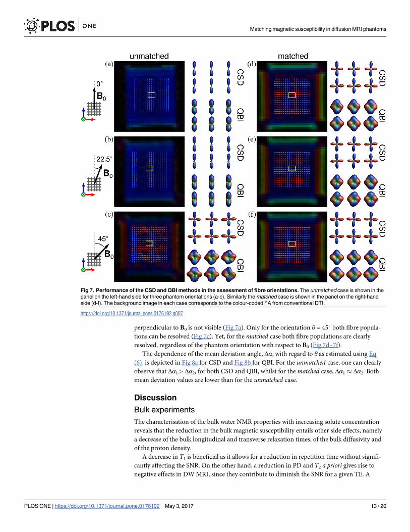
perpendicular to B0 is not visible (Fig 7a). Only for the orientation θ = 45˚ both fibre popula-
tions can be resolved (Fig 7c). Yet, for the matched case both fibre populations are clearly
resolved, regardless of the phantom orientation with respect to B0 (Fig 7d–7f).
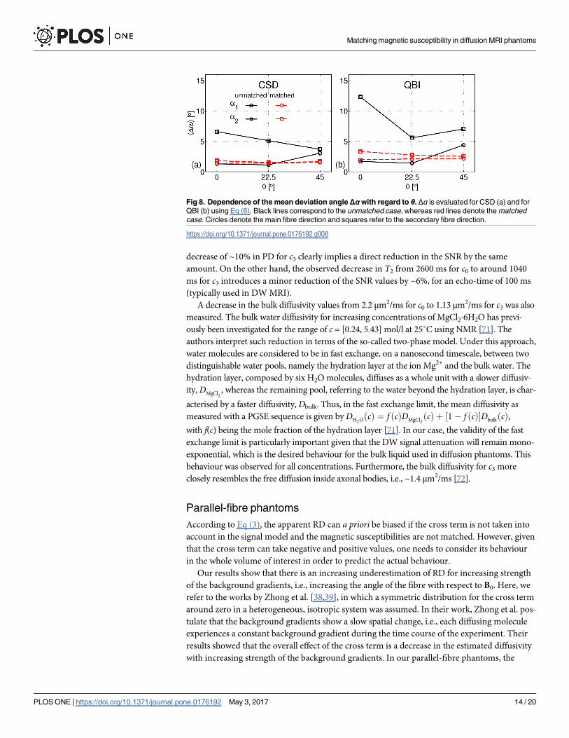
The dependence of the mean deviation angle, Δα, with regard to θ as estimated using Eq
(6), is depicted in Fig 8a for CSD and Fig 8b for QBI. For the unmatched case, one can clearly
observe that Δα1> Δα2, for both CSD and QBI, whilst for the matched case, Δα1� Δα2. Both
mean deviation values are lower than for the unmatched case.
Discussion
Bulk experiments
The characterisation of the bulk water NMR properties with increasing solute concentration
reveals that the reduction in the bulk magnetic susceptibility entails other side effects, namely
a decrease of the bulk longitudinal and transverse relaxation times, of the bulk diffusivity and
of the proton density.
A decrease in T1 is beneficial as it allows for a reduction in repetition time without signifi-
cantly affecting the SNR. On the other hand, a reduction in PD and T2 a priori gives rise to
negative effects in DW MRI, since they contribute to diminish the SNR for a given TE. A
Fig 7. Performance of the CSD and QBI methods in the assessment of fibre orientations. The unmatched case is shown in the
panel on the left-hand side for three phantom orientations (a-c). Similarly the matched case is shown in the panel on the right-hand
side (d-f). The background image in each case corresponds to the colour-coded FA from conventional DTI.
https://doi.org/10.1371/journal.pone.0176192.g007
Matching magnetic susceptibility in diffusion MRI phantoms
PLOS ONE | https://doi.org/10.1371/journal.pone.0176192 May 3, 2017 13 / 20
decrease of ~10% in PD for c3 clearly implies a direct reduction in the SNR by the same
amount. On the other hand, the observed decrease in T2 from 2600 ms for c0 to around 1040
ms for c3 introduces a minor reduction of the SNR values by ~6%, for an echo-time of 100 ms
(typically used in DW MRI).
A decrease in the bulk diffusivity values from 2.2 μm2/ms for c0 to 1.13 μm2/ms for c3 was also
measured. The bulk water diffusivity for increasing concentrations of MgCl2�6H2O has previ-
ously been investigated for the range of c = [0.24, 5.43] mol/l at 25˚C using NMR [71]. The
authors interpret such reduction in terms of the so-called two-phase model. Under this approach,
water molecules are considered to be in fast exchange, on a nanosecond timescale, between two
distinguishable water pools, namely the hydration layer at the ion Mg2+ and the bulk water. The
hydration layer, composed by six H2O molecules, diffuses as a whole unit with a slower diffusiv-
ity, DMgCl2, whereas the remaining pool, referring to the water beyond the hydration layer, is char-
acterised by a faster diffusivity, Dbulk. Thus, in the fast exchange limit, the mean diffusivity as
measured with a PGSE sequence is given by DH2OðcÞ ¼ f ðcÞDMgCl2
ðcÞ þ ½1 � f ðcÞ�DbulkðcÞ,with f(c) being the mole fraction of the hydration layer [71]. In our case, the validity of the fast
exchange limit is particularly important given that the DW signal attenuation will remain mono-
exponential, which is the desired behaviour for the bulk liquid used in diffusion phantoms. This
behaviour was observed for all concentrations. Furthermore, the bulk diffusivity for c3 more
closely resembles the free diffusion inside axonal bodies, i.e., ~1.4 μm2/ms [72].
Parallel-fibre phantoms
According to Eq (3), the apparent RD can a priori be biased if the cross term is not taken into
account in the signal model and the magnetic susceptibilities are not matched. However, given
that the cross term can take negative and positive values, one needs to consider its behaviour
in the whole volume of interest in order to predict the actual behaviour.
Our results show that there is an increasing underestimation of RD for increasing strength
of the background gradients, i.e., increasing the angle of the fibre with respect to B0. Here, we
refer to the works by Zhong et al. [38,39], in which a symmetric distribution for the cross term
around zero in a heterogeneous, isotropic system was assumed. In their work, Zhong et al. pos-
tulate that the background gradients show a slow spatial change, i.e., each diffusing molecule
experiences a constant background gradient during the time course of the experiment. Their
results showed that the overall effect of the cross term is a decrease in the estimated diffusivity
with increasing strength of the background gradients. In our parallel-fibre phantoms, the
Fig 8. Dependence of the mean deviation angleΔαwith regard to θ. Δα is evaluated for CSD (a) and for
QBI (b) using Eq (6). Black lines correspond to the unmatched case, whereas red lines denote the matched
case. Circles denote the main fibre direction and squares refer to the secondary fibre direction.
https://doi.org/10.1371/journal.pone.0176192.g008
Matching magnetic susceptibility in diffusion MRI phantoms
PLOS ONE | https://doi.org/10.1371/journal.pone.0176192 May 3, 2017 14 / 20
diffusion length ld, i.e., the root mean square displacements during TE = 82 ms, was approxi-
mately 12 μm for c0 and 7.5 μm for c8 in the radial direction. On the other hand, considering
the observed mean volume fibre fraction of ~0.64, one can estimate the structural length ls, i.e.,
the distances between the fibres in the interstitial space, to be in the order of 3 μm (assuming a
simple hexagonal arrangement of the lattice as an example). Therefore given that ls is shorter,
the spins cross the pores (structural lengths) many times before dephasing and the magnetic
field inhomogeneities are motionally averaged [73,74]. In other words, the water molecules
experience a mean background gradient with slow spatial change and therefore, a similar argu-
ment to the one utilised by Zhong et al. can be used to explain the observed underestimation
in RD in our work.
The apparent AD should instead ideally remain independent of the orientation as predicted
by Eq (3). This can be observed for concentrations c2-c8. However, AD exhibits a strong under-
estimation for c0 at θ> 45˚, as shown in Fig 4a and 4e. A possible explanation for that could be
the fact that as a result of the strong reduction in T2 due to the strong background gradients,
the SNR reaches very low values (Fig 5). As a consequence, the relative standard deviation
σAD/hADi reaches values of the order of 0.6 to 0.8 (Fig 4i), turning the estimation unreliable.
However, given that all tensor elements were assessed using the asymptotically unbiased ML
estimator, one can expect only a marginal influence of the low SNR in AD. On the other hand,
a stronger influence is expected by the likely presence of some imperfections in the intra-voxel
fibre alignment, which would result in an axial component of the background gradients. More-
over, the difference in magnetic susceptibility between the liquid inside the vial and the sur-
rounding distilled water (see Fig 1, middle phantom), can create long-range field gradients
that can a priori affect the estimation of AD.
Despite the aforementioned results, all parameters remained practically unchanged for the
concentrations c2 and c4. Moreover, as a consequence of the minor reduction in the SNR values,
the relative standard deviation for all parameters remains low across the whole angular range.
Crossing-fibre phantoms
DTI analysis demonstrates that the ellipsoid representation of the diffusion tensor can appear
strongly changed in the presence of background gradients. For the unmatched case and the ori-
entation for θ = 0˚, the tensor eigenvalues follow the relation λ1>λ2�λ3 with λ1 being the diffu-
sivity along the fibre population parallel to B0 (Fig 6a). This relation corresponds to the prolate
shape of the ellipsoid, observed in systems with cylindrical geometry. In other words, only the
fibre population parallel to B0 is observable. This result can be explained by the fact that the
remaining fibre population suffers from a strong reduction in the SNR leading to a strong
underestimation in the diffusivities, similar to that observed in the parallel-fibre phantom for
θ = 90˚ (Fig 4e and 4f). Although the expected oblate shape of the ellipsoid for such fibre con-
figuration, i.e., λ1�λ2>λ3, is recovered for the orientation θ = 45˚, the absolute values of λi are
still biased by the background gradients. The effect on the estimation of the fibre populations
can be more clearly observed in the CSD and QBI analysis in Fig 7a–7c, where both fibre pop-
ulations are recovered only for θ = 45˚.
On the other hand, the dependence of the tensor eigenvalues on the orientation with
respect to B0 is completely suppressed in the matched case, as shown in Fig 6. Similarly, both
fibre populations are clearly identified using CSD and QBI, independently of the phantom ori-
entation. This is even more emphasised by Fig 8, showing that the angular deviations for both
populations are similar and practically independent of the phantom orientation.
Notwithstanding the advantages of the improved design of the phantom, one recognises
several limitations of the fibres themselves regarding their capability for mimicking white
Matching magnetic susceptibility in diffusion MRI phantoms
PLOS ONE | https://doi.org/10.1371/journal.pone.0176192 May 3, 2017 15 / 20
matter tissue properties. One of their intrinsic limitations is that, being rod-like fibres, they
resemble the diffusion properties of only the extracellular space in the white matter tissue.
Moreover, white matter fibres are not perfect cylinders, but their profile is modulated by the
Ranvier nodes, a fact that is not reflected in Dyneema fibres.
Conclusions
In this work we have assessed one of the crucial points in the construction of anisotropic diffu-
sion fibre phantom, namely the necessary independence of the diffusion metrics on the orien-
tation of the phantom in the static magnetic field. We showed that susceptibility differences
between fibre and liquid are responsible for the angular dependence of the diffusion response
signal and consequently of the diffusion parameters and the reconstruction of fibre tracts.
It is demonstrated that an experimentally determined concentration of 1.87 mol/l
MgCl2�6H2O dissolved in distilled water removes the susceptibility difference between the
liquid and the fibres, and hence eliminates the microscopic gradient fields in the interstitial
space. Susceptibility matching leads to complete angular independence of the diffusion metrics
in complex anisotropic diffusion phantoms. This, in turn, allows one to conduct DW MRI
experiments without the need to consider the geometric alignment of the involved structures
with respect to the direction of static magnetic field. Moreover, our findings are of further
interest for the investigation of diffusion in complex scenarios involving susceptibility differ-
ences and local microscopic field gradients.
Supporting information
S1 File. Archive containing results. Datasets are indexed and described in CONTENTS.txt.
(ZIP)
Acknowledgments
The authors thank Mr Michael Schoneck for assistance in the preparation of solutions and Dr.
Nazim Lechea for his help in data processing.
Author Contributions
Conceptualization: EF JL FG AMOP NJS.
Formal analysis: EF JL.
Funding acquisition: NJS.
Investigation: EF JL.
Methodology: EF JL FG AMOP NJS.
Project administration: EF JL.
Resources: EF JL FG NJS.
Software: EF JL.
Supervision: EF JL NJS.
Visualization: EF JL.
Writing – original draft: EF JL.
Writing – review & editing: EF JL FG AMOP NJS.
Matching magnetic susceptibility in diffusion MRI phantoms
PLOS ONE | https://doi.org/10.1371/journal.pone.0176192 May 3, 2017 16 / 20
References1. Bach M, Fritzsche KH, Stieltjes B, Laun FB. Investigation of resolution effects using a specialized diffu-
sion tensor phantom. Magn Reson Med. 2014; 71: 1108–1116. https://doi.org/10.1002/mrm.24774
PMID: 23657980
2. Hubbard PL, Zhou F-L, Eichhorn SJ, Parker GJM. Biomimetic phantom for the validation of diffusion
magnetic resonance imaging. Magn Reson Med. 2015; 73: 299–305. https://doi.org/10.1002/mrm.
25107 PMID: 24469863
3. Lin C-P, Wedeen VJ, Chen J-H, Yao C, Tseng W-YI. Validation of diffusion spectrum magnetic reso-
nance imaging with manganese-enhanced rat optic tracts and ex vivo phantoms. Neuroimage. 2003;
19: 482–495. http://dx.doi.org/10.1016/S1053-8119(03)00154-X PMID: 12880782
4. Laun FB, Huff S, Stieltjes B. On the effects of dephasing due to local gradients in diffusion tensor imag-
ing experiments: relevance for diffusion tensor imaging fiber phantoms. Magn Reson Imaging. 2009;
27: 541–548. http://dx.doi.org/10.1016/j.mri.2008.08.011 PMID: 18977104
5. Watanabe M, Aoki S, Masutani Y, Abe O, Hayashi N, Masumoto T, et al. Flexible ex vivo phantoms for
validation of diffusion tensor tractography on a clinical scanner. Radiat Med. 2006; 24: 605–609. https://
doi.org/10.1007/s11604-006-0076-4 PMID: 17111268
6. Perrin M, Poupon C, Rieul B, Leroux P, Constantinesco A, Mangin J-F, et al. Validation of q-ball imaging
with a diffusion fibre-crossing phantom on a clinical scanner. Philos Trans R Soc London B Biol Sci. The
Royal Society; 2005; 360: 881–891.
7. Descoteaux M, Deriche R, Le Bihan D, Mangin J-F, Poupon C. Multiple q-shell diffusion propagator
imaging. Med Image Anal. 2011; 15: 603–621. http://dx.doi.org/10.1016/j.media.2010.07.001 PMID:
20685153
8. Poupon C, Rieul B, Kezele I, Perrin M, Poupon F, Mangin J-F. New diffusion phantoms dedicated to the
study and validation of high-angular-resolution diffusion imaging (HARDI) models. Magn Reson Med.
2008; 60: 1276–1283. https://doi.org/10.1002/mrm.21789 PMID: 19030160
9. Tournier J-D, Yeh C-H, Calamante F, Cho K-H, Connelly A, Lin C-P. Resolving crossing fibres using
constrained spherical deconvolution: Validation using diffusion-weighted imaging phantom data. Neuro-
image. 2008; 42: 617–625. http://dx.doi.org/10.1016/j.neuroimage.2008.05.002 PMID: 18583153
10. Moussavi-Biugui A, Stieltjes B, Fritzsche K, Semmler W, Laun FB. Novel spherical phantoms for Q-ball
imaging under in vivo conditions. Magn Reson Med. 2011; 65: 190–194. https://doi.org/10.1002/mrm.
22602 PMID: 20740652
11. Wilkins B, Lee N, Gajawelli N, Law M, Lepore N. Fiber estimation and tractography in diffusion MRI:
Development of simulated brain images and comparison of multi-fiber analysis methods at clinical b-val-
ues. Neuroimage. 2015; 109: 341–356. http://dx.doi.org/10.1016/j.neuroimage.2014.12.060 PMID:
25555998
12. Hubbard PL, Parker GJM. Validation of Tractography. In: Johansen-Berg H, Behrens TEJ, editors. Dif-
fusion MRI. Second Edi. San Diego: Academic Press; 2014. pp. 453–480. http://dx.doi.org/10.1016/
B978-0-12-396460-1.00020-2
13. Fillard P, Descoteaux M, Goh A, Gouttard S, Jeurissen B, Malcolm J, et al. Quantitative evaluation of 10
tractography algorithms on a realistic diffusion MR phantom. Neuroimage. 2011; 56: 220–234. http://dx.
doi.org/10.1016/j.neuroimage.2011.01.032 PMID: 21256221
14. Fieremans E, De Deene Y, Delputte S, Ozdemir MS, D’Asseler Y, Vlassenbroeck J, et al. Simulation
and experimental verification of the diffusion in an anisotropic fiber phantom. J Magn Reson. 2008; 190:
189–199. http://dx.doi.org/10.1016/j.jmr.2007.10.014 PMID: 18023218
15. Reischauer C, Staempfli P, Jaermann T, Boesiger P. Construction of a temperature-controlled diffusion
phantom for quality control of diffusion measurements. J Magn Reson Imaging. 2009; 29: 692–698.
https://doi.org/10.1002/jmri.21665 PMID: 19243053
16. Zhu T, Hu R, Qiu X, Taylor M, Tso Y, Yiannoutsos C, et al. Quantification of accuracy and precision of
multi-center DTI measurements: A diffusion phantom and human brain study. Neuroimage. 2011; 56:
1398–1411. http://dx.doi.org/10.1016/j.neuroimage.2011.02.010 PMID: 21316471
17. Chenevert TL, Galban CJ, Ivancevic MK, Rohrer SE, Londy FJ, Kwee TC, et al. Diffusion coefficient
measurement using a temperature-controlled fluid for quality control in multicenter studies. J Magn
Reson Imaging. 2011; 34: 983–987. https://doi.org/10.1002/jmri.22363 PMID: 21928310
18. Lorenz R, Bellemann EM, Hennig J, Il’yasov AK. Anisotropic Phantoms for Quantitative Diffusion Ten-
sor Imaging and Fiber-Tracking Validation. Appl Magn Reson. 2008; 33: 419–429.
19. Yanasak N, Allison J. Use of capillaries in the construction of an MRI phantom for the assessment of dif-
fusion tensor imaging: demonstration of performance. Magn Reson Imaging. 2006; 24: 1349–1361.
http://dx.doi.org/10.1016/j.mri.2006.08.001 PMID: 17145407
Matching magnetic susceptibility in diffusion MRI phantoms
PLOS ONE | https://doi.org/10.1371/journal.pone.0176192 May 3, 2017 17 / 20
20. Fieremans E, De Deene Y, Delputte S, Ozdemir MS, Achten E, Lemahieu I. The design of anisotropic
diffusion phantoms for the validation of diffusion weighted magnetic resonance imaging. Phys Med Biol.
2008; 53: 5405. https://doi.org/10.1088/0031-9155/53/19/009 PMID: 18765890
21. Farrher E, Kaffanke J, Celik AA, Stocker T, Grinberg F, Shah NJ. Novel multisection design of aniso-
tropic diffusion phantoms. Magn Reson Imaging. 2012; 30: 518–526. https://doi.org/10.1016/j.mri.2011.
12.012 PMID: 22285876
22. Jackson JD. Classical electrodynamics. 3rd ed. New York, NY: Wiley; 1999.
23. Majumdar S, Gore JC. Studies of diffusion in random fields produced by variations in susceptibility. J
Magn Reson. 1988; 78: 41–55. http://dx.doi.org/10.1016/0022-2364(88)90155-2
24. Karger J, Pfeifer H, Heink W. Principles and applications of self-diffusion measurements by nuclear
magnetic resonance. In: Waugh J, editor. Advances in Magnetic Resonance. 1250 Sixth Avenue San
Diego, California 92101: Academic Press, Inc.; 1988. pp. 1–89.
25. Goelman G, Prammer MG. The CPMG Pulse Sequence in Strong Magnetic Field Gradients with Appli-
cations to Oil-Well Logging. J Magn Reson Ser A. 1995; 113: 11–18. http://dx.doi.org/10.1006/jmra.
1995.1050
26. Beaulieu C, Allen PS. An in vitro evaluation of the effects of local magnetic-susceptibility-induced gradi-
ents on anisotropic water diffusion in nerve. Magn Reson Med. 1996; 36: 39–44. PMID: 8795018
27. De Santis S, Rebuzzi M, Di Pietro G, Fasano F, Maraviglia B, Capuani S. In vitro and in vivo MR evalua-
tion of internal gradient to assess trabecular bone density. Phys Med Biol. 2010; 55: 5767. https://doi.
org/10.1088/0031-9155/55/19/010 PMID: 20844335
28. Clark CA, Barker GJ, Tofts PS. An in Vivo Evaluation of the Effects of Local Magnetic Susceptibility-
Induced Gradients on Water Diffusion Measurements in Human Brain. J Magn Reson. 1999; 141: 52–
61. http://dx.doi.org/10.1006/jmre.1999.1872 PMID: 10527743
29. Palombo M, Gentili S, Bozzali M, Macaluso E, Capuani S. New insight into the contrast in diffusional
kurtosis images: Does it depend on magnetic susceptibility? Magn Reson Med. 2015; 73: 2015–2024.
https://doi.org/10.1002/mrm.25308 PMID: 24894844
30. Lindemeyer J, Oros-Peusquens A-M, Farrher E, Grinberg F, Shah NJ. Orientation and Microstructure
Effects on Susceptibility Reconstruction: a Diffusion Phantom Study. Proceedings of the International
Society for Magnetic Resonance in Medicine. 2011. p. 4516.
31. Stejskal EO, Tanner JE. Spin Diffusion Measurements: Spin Echoes in the Presence of a Time Depen-
dent Field Gradient. J Chem Phys. 1965; 42.
32. Capuani S, Piccirilli E, Di Pietro G, Celi M, Tarantino U. Microstructural differences between osteopo-
rotic and osteoarthritic femoral cancellous bone: an in vitro magnetic resonance micro-imaging investi-
gation. Aging Clin Exp Res. 2013; 25: 51–54.
33. Rebuzzi M, Vinicola V, Taggi F, Sabatini U, Wehrli FW, Capuani S. Potential diagnostic role of the MRI-
derived internal magnetic field gradient in calcaneus cancellous bone for evaluating postmenopausal
osteoporosis at 3 T. Bone. 2013; 57: 155–163. http://dx.doi.org/10.1016/j.bone.2013.07.027 PMID:
23899635
34. Packer KJ. The effects of diffusion through locally inhomogeneous magnetic fields on transverse
nuclear spin relaxation in heterogeneous systems. Proton transverse relaxation in striated muscle tis-
sue. J Magn Reson. 1973; 9: 438–443. http://dx.doi.org/10.1016/0022-2364(73)90186-8
35. Knight MJ, Kauppinen RA. Diffusion-mediated nuclear spin phase decoherence in cylindrically porous
materials. J Magn Reson. 2016; 269: 1–12. http://dx.doi.org/10.1016/j.jmr.2016.05.007 PMID:
27208416
36. Le Bihan D, Mangin J-F, Poupon C, Clark CA, Pappata S, Molko N, et al. Diffusion tensor imaging: Con-
cepts and applications. J Magn Reson Imaging. John Wiley & Sons, Inc.; 2001; 13: 534–546.
37. Miller AJ, Joseph PM. The use of power images to perform quantitative analysis on low SNR MR
images. Magn Reson Imaging. 1993; 11: 1051–1056. PMID: 8231670
38. Zhong J, Gore JC. Studies of restricted diffusion in heterogeneous media containing variations in sus-
ceptibility. Magn Reson Med. 1991; 19: 276–284. PMID: 1881316
39. Zhong J, Kennan RP, Gore JC. Effects of susceptibility variations on NMR measurements of diffusion. J
Magn Reson. 1991; 95: 267–280. http://dx.doi.org/10.1016/0022-2364(91)90217-H
40. Kiselev VG. Effect of magnetic field gradients induced by microvasculature on NMR measurements of
molecular self-diffusion in biological tissues. J Magn Reson. 2004; 170: 228–235. http://dx.doi.org/10.
1016/j.jmr.2004.07.004 PMID: 15388085
41. Chen WC, Foxley S, Miller KL. Detecting microstructural properties of white matter based on compart-
mentalization of magnetic susceptibility. Neuroimage. Elsevier Inc.; 2013; 70: 1–9.
Matching magnetic susceptibility in diffusion MRI phantoms
PLOS ONE | https://doi.org/10.1371/journal.pone.0176192 May 3, 2017 18 / 20
42. Lee J, Shmueli K, Fukunaga M, van Gelderen P, Merkle H, Silva AC, et al. Sensitivity of MRI resonance
frequency to the orientation of brain tissue microstructure. Proc Natl Acad Sci U S A. 2010; 107: 5130–
5135. https://doi.org/10.1073/pnas.0910222107 PMID: 20202922
43. Caporale A, Palombo M, Macaluso E, Guerreri M, Bozzali M, Capuani S. The γ-parameter of anoma-
lous diffusion quantified in human brain by MRI depends on local magnetic susceptibility differences.
Neuroimage. 2017; 147: 619–631. http://dx.doi.org/10.1016/j.neuroimage.2016.12.051 PMID:
28011255
44. Duyn JH, van Gelderen P, Li T-Q, de Zwart J a, Koretsky AP, Fukunaga M. High-field MRI of brain corti-
cal substructure based on signal phase. Proc Natl Acad Sci U S A. 2007; 104: 11796–11801. https://
doi.org/10.1073/pnas.0610821104 PMID: 17586684
45. Liu C. Susceptibility tensor imaging. Magn Reson Med. 2010; 63: 1471–1477. https://doi.org/10.1002/
mrm.22482 PMID: 20512849
46. Zheng G, Price WS. Suppression of background gradients in (B0 gradient-based) NMR diffusion experi-
ments. Concepts Magn Reson Part A. 2007; 30A: 261–277.
47. Meiboom S, Gill D. Modified Spin Echo Method for Measuring Nuclear Relaxation Times. Rev Sci
Instrum. 1958; 29.
48. Sun PZ, Seland JG, Cory D. Background gradient suppression in pulsed gradient stimulated echo mea-
surements. J Magn Reson. 2003; 161: 168–173. PMID: 12713966
49. Ballon D, Mahmood U, Jakubowski A, Koutcher JA. Resolution enhanced NMR spectroscopy in biologi-
cal systems via magnetic susceptibility matched sample immersion chambers. Magn Reson Med.
1993; 30: 754–758. PMID: 8139459
50. Tournier J-D, Calamante F, Connelly A. Robust determination of the fibre orientation distribution in diffu-
sion MRI: Non-negativity constrained super-resolved spherical deconvolution. Neuroimage. 2007; 35:
1459–1472. http://dx.doi.org/10.1016/j.neuroimage.2007.02.016 PMID: 17379540
51. Tuch DS. Q-ball imaging. Magn Reson Med. Wiley Subscription Services, Inc., A Wiley Company;
2004; 52: 1358–1372.
52. Sijbers J, den Dekker AJ. Maximum likelihood estimation of signal amplitude and noise variance from
MR data. Magn Reson Med. 2004; 51: 586–594. https://doi.org/10.1002/mrm.10728 PMID: 15004801
53. Schenck JF. The role of magnetic susceptibility in magnetic resonance imaging: MRI magnetic compati-
bility of the first and second kinds. Med Phys. 1996; 23.
54. Haynes WM, editor. CRC Handbook of Chemistry and Physics—Electrical Conductivity of Aqueous
Solutions. 70th ed. CRC Press, Boca Raton; 1989.
55. Lide DR, editor. CRC Handbook of Chemistry and Physics, Internet Version 2005 [Internet]. CRC
Press, Boca Raton, FL; 2005. http://www.hbcpnetbase.com
56. Reichenbach JR. The future of susceptibility contrast for assessment of anatomy and function. Neuro-
image. 2012; 62: 1311–1315. http://dx.doi.org/10.1016/j.neuroimage.2012.01.004 PMID: 22245644
57. Wang Y, Liu T. Quantitative susceptibility mapping (QSM): Decoding MRI data for a tissue magnetic
biomarker. Magn Reson Med. 2015; 73: 82–101. https://doi.org/10.1002/mrm.25358 PMID: 25044035
58. Haacke EM, Brown RW, Thompson MR, Venkatesan R, others. Magnetic resonance imaging: physical
principles and sequence design. New York: Wiley; 1999.
59. Lindemeyer J, Oros-Peusquens A-M, Shah NJ. Multistage Background Field Removal (MUBAFIRE)—
Compensating for B0 Distortions at Ultra-High Field. PLoS One. 2015; 10: e0138325. https://doi.org/10.
1371/journal.pone.0138325 PMID: 26393515
60. Koch KM, Papademetris X, Rothman DL, de Graaf RA. Rapid calculations of susceptibility-induced
magnetostatic field perturbations for in vivo magnetic resonance. Phys Med Biol. 2006; 51: 6381.
https://doi.org/10.1088/0031-9155/51/24/007 PMID: 17148824
61. Marques JP, Bowtell R. Application of a Fourier-based method for rapid calculation of field inhomogene-
ity due to spatial variation of magnetic susceptibility. Concepts Magn Reson Part B Magn Reson Eng.
2005; 25B: 65–78.
62. Shah NJ, Zaitsev M, Steinhoff S, Zilles K. A New Method for Fast Multislice T1 Mapping. Neuroimage.
2001; 14: 1175–1185. http://dx.doi.org/10.1006/nimg.2001.0886 PMID: 11697949
63. Reese TG, Heid O, Weisskoff RM, Wedeen VJ. Reduction of eddy-current-induced distortion in diffu-
sion MRI using a twice-refocused spin echo. Magn Reson Med. 2003; 49: 177–182. https://doi.org/10.
1002/mrm.10308 PMID: 12509835
64. Smith SM, Jenkinson M, Woolrich MW, Beckmann CF, Behrens TEJ, Johansen-Berg H, et al.
Advances in functional and structural MR image analysis and implementation as FSL. Neuroimage.
2004; 23, Supple: S208–S219. http://dx.doi.org/10.1016/j.neuroimage.2004.07.051
Matching magnetic susceptibility in diffusion MRI phantoms
PLOS ONE | https://doi.org/10.1371/journal.pone.0176192 May 3, 2017 19 / 20
65. Woolrich MW, Jbabdi S, Patenaude B, Chappell M, Makni S, Behrens T, et al. Bayesian analysis of neu-
roimaging data in FSL. Neuroimage. 2009; 45: S173–S186. http://dx.doi.org/10.1016/j.neuroimage.
2008.10.055 PMID: 19059349
66. Jenkinson M, Smith S. A global optimisation method for robust affine registration of brain images. Med
Image Anal. 2001; 5: 143–156. http://dx.doi.org/10.1016/S1361-8415(01)00036-6 PMID: 11516708
67. Leemans A, Jones DK. The B-matrix must be rotated when correcting for subject motion in DTI data.
Magn Reson Med. 2009; 61: 1336–1349. https://doi.org/10.1002/mrm.21890 PMID: 19319973
68. Leemans A, Jeurissen B, Sijbers J, Jones DK. ExploreDTI: a graphical toolbox for processing, analyz-
ing, and visualizing diffusion MR data. Proc Intl Soc Mag Reson Med. 2009. p. 3537.
69. Jeurissen B, Leemans A, Tournier J-D, Jones DK, Sijbers J. Investigating the prevalence of complex
fiber configurations in white matter tissue with diffusion magnetic resonance imaging. Hum Brain Mapp.
2013; 34: 2747–2766. https://doi.org/10.1002/hbm.22099 PMID: 22611035
70. Aja-Fernandez S, Tristan-Vega A, Alberola-Lopez C. Noise estimation in single- and multiple-coil mag-
netic resonance data based on statistical models. Magn Reson Imaging. 2009; 27: 1397–1409. http://
dx.doi.org/10.1016/j.mri.2009.05.025 PMID: 19570640
71. Struis RPWJ, De Bleijser J, Leyte JC. An NMR contribution to the interpretation of the dynamical behav-
ior of water molecules as a function of the magnesium chloride concentration at 25.degree.C. J Phys
Chem. 1987; 91: 6309–6315.
72. Barazany D, Basser PJ, Assaf Y. In vivo measurement of axon diameter distribution in the corpus callo-
sum of rat brain. Brain. 2009; 132: 1210–1220. Available: http://dx.doi.org/10.1093/brain/awp042
PMID: 19403788
73. Mitchell J, Chandrasekera TC, Johns ML, Gladden LF, Fordham EJ. Nuclear magnetic resonance
relaxation and diffusion in the presence of internal gradients: The effect of magnetic field strength. Phys
Rev E. American Physical Society; 2010; 81: 26101.
74. Di Pietro G, Palombo M, Capuani S. Internal Magnetic Field Gradients in Heterogeneous Porous Sys-
tems: Comparison Between Spin-Echo and Diffusion Decay Internal Field (DDIF) Method. Appl Magn
Reson. 2014; 45: 771–784.
Matching magnetic susceptibility in diffusion MRI phantoms
PLOS ONE | https://doi.org/10.1371/journal.pone.0176192 May 3, 2017 20 / 20