Concrete Semanticsconcrete-semantics.org/slides-isabelle.pdf · 2019-10-14 · Why Semantics? Without semantics, we do not really know what our programs mean. We merely have a good

Concrete Semanticswith Isabelle/HOL

Tobias Nipkow

Fakultat fur InformatikTechnische Universitat Munchen

2019-10-14

1

Chapter 1

Introduction

2

1 Background

2 This Course

3

1 Background

2 This Course

4

Why Semantics?

Without semantics,we do not really know what our programs mean.

We merely have a good intuition and a warm feeling.

Like the state of mathematics in the 19th century— before set theory and logic entered the scene.

5

Intuition is important!

• You need a good intuition to get your work doneefficiently.

• To understand the average accounting program,intuition suffices.

• To write a bug-free accounting program may requiremore than intuition!

• I assume you have the necessary intuition.

• This course is about “beyond intuition”.

6

Intuition is not sufficient!

Writing correct language processors (e.g. compilers,refactoring tools, . . . ) requires

• a deep understanding of language semantics,

• the ability to reason (= perform proofs) about thelanguage and your processor.

Example:What does the correctness of a type checker even mean?How is it proved?

7

Why Semantics??

We have a compiler — that is the ultimate semantics!!

• A compiler gives each individual program asemantics.

• It does not help with reasoning about the PL orindividual programs.

• Because compilers are far too complicated.

• They provide the worst possible semantics.

• Moreover: compilers may differ!

8

The sad facts of life

• Most languages have one or more compilers.

• Most compilers have bugs.

• Few languages have a (separate, abstract)semantics.

• If they do, it will be informal (English).

9

Bugs

• Google “compiler bug”

• Google “hostile applet”Early versions of Java had various security holes.Some of them had to do with an incorrectbytecode verifier.

GI Dissertationspreis 2003:Gerwin Klein: Verified Java Bytecode Verification

10

Standard ML (SML)First real language with a mathematical semantics:Milner, Tofte, Harper:The Definition of Standard ML. 1990.

Robin Milner (1934–2010)Turing Award 1991.

Main achievements: LCF (theorem proving)SML (functional programming)CCS, pi (concurrency)

11

The sad fact of life

SML semantics hardly used:

• too difficult to read to answer simple questionsquickly

• too much detail to allow reliable informal proof

• not processable beyond LATEX, not even executable

12

More sad facts of life

• Real programming languages are complex.

• Even if designed by academics, not industry.

• Complex designs are error-prone.

• Informal mathematical proofs of complex designsare also error-prone.

13

The solution

Machine-checked language semantics and proofs

• Semantics at least type-correct

• Maybe executable

• Proofs machine-checked

The tool:

Proof Assistant (PA)or

Interactive Theorem Prover (ITP)

14

Proof Assistants

• You give the structure of the proof

• The PA checks the correctness of each step

• Can prove hard and huge theorems

Government health warnings:

Time consumingPotentially addictive

Undermines your naive trust in informal proofs

15

Terminology

This lecture course:

Formal = machine-checkedVerification = formal correctness proof

Traditionally:

Formal = mathematical

16

Two landmark verifications

C compilerCompetitive with gcc -O1

Xavier LeroyINRIA Parisusing Coq

Operating systemmicrokernel (L4)

Gerwin Klein (& Co)NICTA Sydneyusing Isabelle

17

A happy fact of life

Programming language researchersare increasingly using PAs

18

Why verification pays off

Short term: The software works!

Long term:

Tracking effects of changes by rerunning proofs

Incremental changes of the softwaretypically require only incremental changes of the proofs

Long term much more important than short term:

Software Never Dies

19

1 Background

2 This Course

20

What this course is not about

• Hot or trendy PLs

• Comparison of PLs or PL paradigms

• Compilers (although they will be one application)

21

What this course is about

• Techniques for the description and analysis of• PLs• PL tools• Programs

• Description techniques: operational semantics

• Proof techniques: inductions

Both informally and formally (PA!)

22

Our PA: Isabelle/HOL

• Started 1986 by Paulson (U of Cambridge)

• Later development mainly byNipkow & Co (TUM) and Wenzel

• The logic HOL is ordinary mathematics

Learning to use Isabelle/HOLis an integral part of the course

All exercises require the use of Isabelle/HOL

23

Why I am so passionateabout the PA part

• It is the future

• It is the only way to deal with complex languagesreliably

• I want students to learn how to write correct proofs

• I have seen too many proofs that look more likeLSD trips than coherent mathematical arguments

24

Overview of course

• Introduction to Isabelle/HOL

• IMP (assignment and while loops) and its semantics

• A compiler for IMP

• Hoare logic for IMP

• Type systems for IMP

• Program analysis for IMP

25

The semantics part of the course is mostly traditional

The use of a PA is leading edge

A growing number of universities offer related course

26

What you learn in this course goes far beyond PLs

It has applications in compilers, security,software engineering etc.

It is a new approach to informatics

27

Part I

Isabelle

29

Chapter 2

Programming and Proving

30

3 Overview of Isabelle/HOL

4 Type and function definitions

5 Induction Heuristics

6 Simplification

31

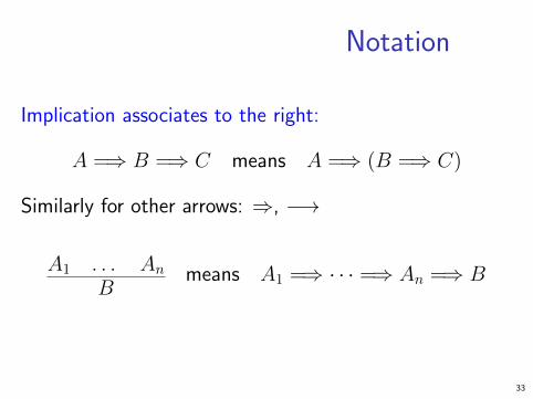
Notation

Implication associates to the right:

A =⇒ B =⇒ C means A =⇒ (B =⇒ C)

Similarly for other arrows: ⇒, −→

A1 . . . An

Bmeans A1 =⇒ · · · =⇒ An =⇒ B

33




6 Simplification

34

HOL = Higher-Order LogicHOL = Functional Programming + Logic

HOL has• datatypes• recursive functions• logical operators

HOL is a programming language!

Higher-order = functions are values, too!

HOL Formulas:• For the moment: only term = term,

e.g. 1 + 2 = 4• Later: ∧, ∨, −→, ∀, . . .

35

3 Overview of Isabelle/HOLTypes and termsInterfaceBy example: types bool, nat and listSummary

36

Types

Basic syntax:

τ ::= (τ)| bool | nat | int | . . . base types| ′a | ′b | . . . type variables| τ ⇒ τ functions| τ × τ pairs (ascii: *)| τ list lists| τ set sets| . . . user-defined types

Convention: τ 1 ⇒ τ 2 ⇒ τ 3 ≡ τ 1 ⇒ (τ 2 ⇒ τ 3)

37

Terms

Terms can be formed as follows:

• Function application: f tis the call of function f with argument t.If f has more arguments: f t1 t2 . . .Examples: sin π, plus x y

• Function abstraction: λx. tis the function with parameter x and result t,i.e. “x 7→ t ”.Example: λx. plus x x

38

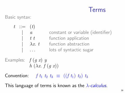
TermsBasic syntax:

t ::= (t)| a constant or variable (identifier)| t t function application| λx. t function abstraction| . . . lots of syntactic sugar

Examples: f (g x) yh (λx. f (g x))

Convention: f t1 t2 t3 ≡ ((f t1) t2) t3

This language of terms is known as the λ-calculus.39

The computation rule of the λ-calculus is thereplacement of formal by actual parameters:

(λx. t) u = t[u/x]

where t[u/x] is “t with u substituted for x”.

Example: (λx. x + 5) 3 = 3 + 5

• The step from (λx. t) u to t[u/x] is calledβ-reduction.

• Isabelle performs β-reduction automatically.

40

Terms must be well-typed

(the argument of every function call must be of the right type)

Notation:t :: τ means “t is a well-typed term of type τ”.

t :: τ 1 ⇒ τ 2 u :: τ 1t u :: τ 2

41

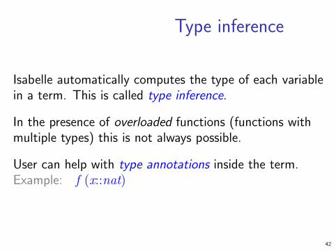
Type inference

Isabelle automatically computes the type of each variablein a term. This is called type inference.

In the presence of overloaded functions (functions withmultiple types) this is not always possible.

User can help with type annotations inside the term.Example: f (x::nat)

42

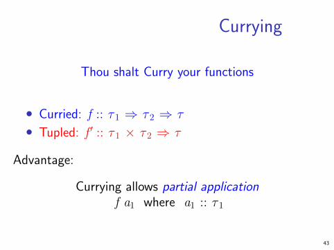
Currying

Thou shalt Curry your functions

• Curried: f :: τ 1 ⇒ τ 2 ⇒ τ

• Tupled: f ′ :: τ 1 × τ 2 ⇒ τ

Advantage:

Currying allows partial applicationf a1 where a1 :: τ 1

43

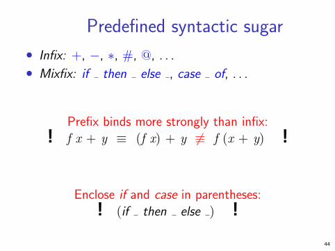
Predefined syntactic sugar

• Infix: +, −, ∗, #, @, . . .

• Mixfix: if then else , case of, . . .

Prefix binds more strongly than infix:

! f x + y ≡ (f x) + y 6≡ f (x + y) !

Enclose if and case in parentheses:

! (if then else ) !

44

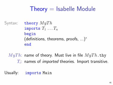
Theory = Isabelle Module

Syntax: theory MyThimports T1 . . .Tnbegin

(definitions, theorems, proofs, ...)∗

end

MyTh: name of theory. Must live in file MyTh.thy

Ti: names of imported theories. Import transitive.

Usually: imports Main

45

Concrete syntax

In .thy files:Types, terms and formulas need to be inclosed in "

Except for single identifiers

" normally not shown on slides

46


47

isabelle jedit

• Based on jEdit editor

• Processes Isabelle text automaticallywhen editing .thy files (like modern Java IDEs)

48

Overview_Demo.thy

49


50

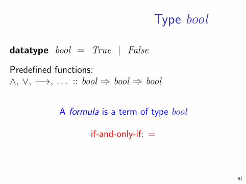
Type bool

datatype bool = True | False

Predefined functions:∧, ∨, −→, . . . :: bool ⇒ bool ⇒ bool

A formula is a term of type bool

if-and-only-if: =

51

Type nat

datatype nat = 0 | Suc nat

Values of type nat: 0, Suc 0, Suc(Suc 0), . . .

Predefined functions: +, ∗, ... :: nat ⇒ nat ⇒ nat

! Numbers and arithmetic operations are overloaded:0,1,2,... :: ′a, + :: ′a ⇒ ′a ⇒ ′a

You need type annotations: 1 :: nat, x + (y::nat)unless the context is unambiguous: Suc z

52

Nat_Demo.thy

53

An informal proof

Lemma add m 0 = mProof by induction on m.

• Case 0 (the base case):add 0 0 = 0 holds by definition of add.

• Case Suc m (the induction step):We assume add m 0 = m,the induction hypothesis (IH).We need to show add (Suc m) 0 = Suc m.The proof is as follows:add (Suc m) 0 = Suc (add m 0) by def. of add

= Suc m by IH

54

Type ′a list

Lists of elements of type ′a

datatype ′a list = Nil | Cons ′a ( ′a list)

Some lists: Nil, Cons 1 Nil, Cons 1 (Cons 2 Nil), . . .

Syntactic sugar:

• [] = Nil: empty list

• x # xs = Cons x xs:list with first element x (“head”) and rest xs (“tail”)

• [x1, . . . , xn] = x1 # . . . xn # []

55

Structural Induction for lists

To prove that P(xs) for all lists xs, prove

• P([]) and

• for arbitrary but fixed x and xs,P(xs) implies P(x#xs).

P([])∧x xs. P(xs) =⇒ P(x#xs)

P(xs)

56

List_Demo.thy

57

An informal proofLemma app (app xs ys) zs = app xs (app ys zs)Proof by induction on xs.• Case Nil: app (app Nil ys) zs = app ys zs =app Nil (app ys zs) holds by definition of app.• Case Cons x xs: We assume app (app xs ys) zs =app xs (app ys zs) (IH), and we need to showapp (app (Cons x xs) ys) zs =app (Cons x xs) (app ys zs).The proof is as follows:app (app (Cons x xs) ys) zs= Cons x (app (app xs ys) zs) by definition of app= Cons x (app xs (app ys zs)) by IH= app (Cons x xs) (app ys zs) by definition of app

58

Large library: HOL/List.thy

Included in Main.

Don’t reinvent, reuse!

Predefined: xs @ ys (append), length, and map

59


60

• datatype defines (possibly) recursive data types.

• fun defines (possibly) recursive functions bypattern-matching over datatype constructors.

61

Proof methods

• induction performs structural induction on somevariable (if the type of the variable is a datatype).

• auto solves as many subgoals as it can, mainly bysimplification (symbolic evaluation):

“=” is used only from left to right!

62

Proofs

General schema:

lemma name: "..."

apply (...)

apply (...)...done

If the lemma is suitable as a simplification rule:

lemma name[simp]: "..."

63

Top down proofs

Command

sorry

“completes” any proof.

Allows top down development:

Assume lemma first, prove it later.

64

The proof state

1.∧

x1 . . . xp. A =⇒ B

x1 . . . xp fixed local variablesA local assumption(s)B actual (sub)goal

65

Multiple assumptions

[[ A1; . . . ; An ]] =⇒ B

abbreviates

A1 =⇒ . . . =⇒ An =⇒ B

; ≈ “and”

66




6 Simplification

67

4 Type and function definitionsType definitionsFunction definitions

68

Type synonymstype_synonym name = τ

Introduces a synonym name for type τ

Examples

type_synonym string = char list

type_synonym ( ′a, ′b)foo = ′a list × ′b list

Type synonyms are expanded after parsingand are not present in internal representation and output

69

datatype — the general casedatatype (α1, . . . , αn)t = C1 τ1,1 . . . τ1,n1

| . . .| Ck τk,1 . . . τk,nk

• Types: Ci :: τi,1 ⇒ · · · ⇒ τi,ni⇒ (α1, . . . , αn)t

• Distinctness: Ci . . . 6= Cj . . . if i 6= j

• Injectivity: (Ci x1 . . . xni= Ci y1 . . . yni

) =(x1 = y1 ∧ · · · ∧ xni

= yni)

Distinctness and injectivity are applied automaticallyInduction must be applied explicitly

70

Case expressionsDatatype values can be taken apart with case:

(case xs of [] ⇒ . . . | y#ys ⇒ ... y ... ys ...)

Wildcards:

(case m of 0 ⇒ Suc 0 | Suc ⇒ 0)

Nested patterns:

(case xs of [0] ⇒ 0 | [Suc n] ⇒ n | ⇒ 2)

Complicated patterns mean complicated proofs!

Need ( ) in context

71

Tree_Demo.thy

72

The option type

datatype ′a option = None | Some ′a

If ′a has values a1, a2, . . .then ′a option has values None, Some a1, Some a2, . . .

Typical application:

fun lookup :: ( ′a × ′b) list ⇒ ′a ⇒ ′b option wherelookup [] x = None |lookup ((a, b) # ps) x =

(if a = x then Some b else lookup ps x)

73

4 Type and function definitionsType definitionsFunction definitions

74

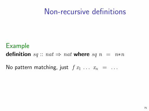
Non-recursive definitions

Exampledefinition sq :: nat ⇒ nat where sq n = n∗n

No pattern matching, just f x1 . . . xn = . . .

75

The danger of nontermination

How about f x = f x + 1 ?

Subtract f x on both sides.=⇒ 0 = 1

! All functions in HOL must be total !

76

Key features of fun

• Pattern-matching over datatype constructors

• Order of equations matters

• Termination must be provable automaticallyby size measures

• Proves customized induction schema

77

Example: separation

fun sep :: ′a ⇒ ′a list ⇒ ′a list wheresep a (x#y#zs) = x # a # sep a (y#zs) |sep a xs = xs

78

Example: Ackermann

fun ack :: nat ⇒ nat ⇒ nat whereack 0 n = Suc n |ack (Suc m) 0 = ack m (Suc 0) |ack (Suc m) (Suc n) = ack m (ack (Suc m) n)

Terminates because the arguments decreaselexicographically with each recursive call:

• (Suc m, 0) > (m, Suc 0)

• (Suc m, Suc n) > (Suc m, n)

• (Suc m, Suc n) > (m, )

79

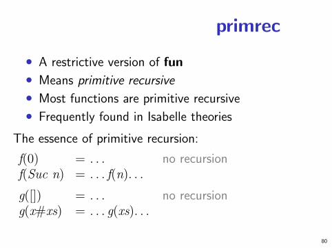
primrec

• A restrictive version of fun

• Means primitive recursive

• Most functions are primitive recursive

• Frequently found in Isabelle theories

The essence of primitive recursion:

f(0) = . . . no recursionf(Suc n) = . . . f(n). . .

g([]) = . . . no recursiong(x#xs) = . . . g(xs). . .

80




6 Simplification

81

Basic induction heuristics

Theorems about recursive functionsare proved by induction

Induction on argument number i of fif f is defined by recursion on argument number i

82

A tail recursive reverse

Our initial reverse:

fun rev :: ′a list ⇒ ′a list whererev [] = [] |rev (x#xs) = rev xs @ [x]

A tail recursive version:

fun itrev :: ′a list ⇒ ′a list ⇒ ′a list whereitrev [] ys = ys |itrev (x#xs) ys =

itrev xs (x#ys)

lemma itrev xs [] = rev xs

83

Induction_Demo.thy

Generalisation

84

Generalisation

• Replace constants by variables

• Generalize free variables• by arbitrary in induction proof• (or by universal quantifier in formula)

85

So far, all proofs were by structural inductionbecause all functions were primitive recursive.

In each induction step, 1 constructor is added.In each recursive call, 1 constructor is removed.

Now: induction for complex recursion patterns.

86

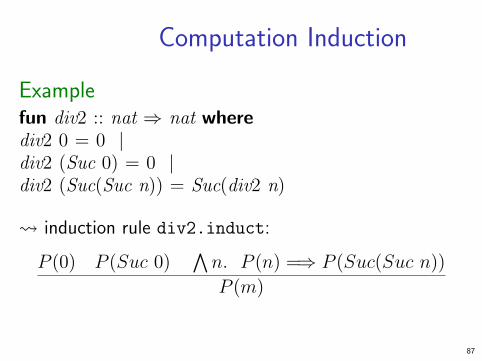
Computation Induction

Examplefun div2 :: nat ⇒ nat wherediv2 0 = 0 |div2 (Suc 0) = 0 |div2 (Suc(Suc n)) = Suc(div2 n)

induction rule div2.induct:

P (0) P (Suc 0)∧n. P (n) =⇒ P (Suc(Suc n))

P (m)

87


If f :: τ ⇒ τ ′ is defined by fun, a special inductionschema is provided to prove P (x) for all x :: τ :

for each defining equation

f(e) = . . . f(r1) . . . f(rk) . . .

prove P (e) assuming P (r1), . . . , P (rk).

Induction follows course of (terminating!) computationMotto: properties of f are best proved by rule f.induct

88

How to apply f.induct

If f :: τ1 ⇒ · · · ⇒ τn ⇒ τ ′:

(induction a1 . . . an rule: f.induct)

Heuristic:

• there should be a call f a1 . . . an in your goal

• ideally the ai should be variables.

89

Induction_Demo.thy


90




6 Simplification

91

Simplification means . . .

Using equations l = r from left to right

As long as possible

Terminology: equation simplification rule

Simplification = (Term) Rewriting

92

An example

Equations:

0 + n = n (1)(Suc m) + n = Suc (m+ n) (2)

(Suc m ≤ Suc n) = (m ≤ n) (3)(0 ≤ m) = True (4)

Rewriting:

0 + Suc 0 ≤ Suc 0 + x(1)=

Suc 0 ≤ Suc 0 + x(2)=

Suc 0 ≤ Suc (0 + x)(3)=

0 ≤ 0 + x(4)=

True93

Conditional rewriting

Simplification rules can be conditional:

[[ P1; . . . ; Pk ]] =⇒ l = r

is applicable only if all Pi can be proved first,again by simplification.

Examplep(0) = True

p(x) =⇒ f(x) = g(x)

We can simplify f(0) to g(0) butwe cannot simplify f(1) because p(1) is not provable.

94

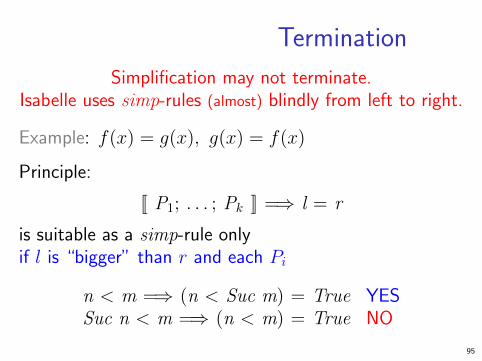
Termination

Simplification may not terminate.Isabelle uses simp-rules (almost) blindly from left to right.

Example: f(x) = g(x), g(x) = f(x)

Principle:

[[ P1; . . . ; Pk ]] =⇒ l = r

is suitable as a simp-rule onlyif l is “bigger” than r and each Pi

n < m =⇒ (n < Suc m) = True YESSuc n < m =⇒ (n < m) = True NO

95

Proof method simpGoal: 1. [[ P1; . . . ; Pm ]] =⇒ C

apply(simp add: eq1 . . . eqn)

Simplify P1 . . . Pm and C using

• lemmas with attribute simp

• rules from fun and datatype

• additional lemmas eq1 . . . eqn• assumptions P1 . . . Pm

Variations:

• (simp . . . del: . . . ) removes simp-lemmas

• add and del are optional96

auto versus simp

• auto acts on all subgoals

• simp acts only on subgoal 1

• auto applies simp and more

• auto can also be modified:(auto simp add: . . . simp del: . . . )

97

Rewriting with definitions

Definitions (definition) must be used explicitly:

(simp add: f def . . . )

f is the function whose definition is to be unfolded.

98

Case splitting with simp/autoAutomatic:

P (if A then s else t)=

(A −→ P(s)) ∧ (¬A −→ P(t))

By hand:

P (case e of 0 ⇒ a | Suc n ⇒ b)=

(e = 0 −→ P(a)) ∧ (∀ n. e = Suc n −→ P(b))

Proof method: (simp split: nat.split)Or auto. Similar for any datatype t: t.split

99

Simp_Demo.thy

100

Chapter 3

Case Study: IMP Expressions

101

7 Case Study: IMP Expressions

102

7 Case Study: IMP Expressions

103

This section introduces

arithmetic and boolean expressions

of our imperative language IMP.

IMP commands are introduced later.

104

7 Case Study: IMP ExpressionsArithmetic ExpressionsBoolean ExpressionsStack Machine and Compilation

105

Concrete and abstract syntax

Concrete syntax: strings, eg "a+5*b"

Abstract syntax: trees, eg+@@@

��a *

AAA

��

5 b

Parser: function from strings to trees

Linear view of trees: terms, eg Plus a (Times 5 b)

Abstract syntax trees/terms are datatype values!

106

Concrete syntax is defined by a context-free grammar, eg

a ::= n | x | (a) | a+ a | a ∗ a | . . .

where n can be any natural number and x any variable.

We focus on abstract syntaxwhich we introduce via datatypes.

107

Datatype aexp

Variable names are strings, values are integers:

type_synonym vname = stringdatatype aexp = N int | V vname | Plus aexp aexp

Concrete Abstract5 N 5x V ′′x ′′

x+y Plus (V ′′x ′′) (V ′′y ′′)2+(z+3) Plus (N 2) (Plus (V ′′z ′′) (N 3))

108

Warning

This is syntax, not (yet) semantics!

N 0 6= Plus (N 0) (N 0)

109

The (program) state

What is the value of x+1?

• The value of an expressiondepends on the value of its variables.

• The value of all variables is recorded in the state.

• The state is a function from variable names tovalues:

type_synonym val = inttype_synonym state = vname ⇒ val

110

Function update notation

If f :: τ 1 ⇒ τ 2 and a :: τ 1 and b :: τ 2 then

f(a := b)

is the function that behaves like fexcept that it returns b for argument a.

f(a := b) = (λx. if x = a then b else f x)

111

How to write down a state

Some states:

• λx. 0

• (λx. 0)( ′′a ′′ := 3)

• ((λx. 0)( ′′a ′′ := 5))( ′′x ′′ := 3)

Nicer notation:

< ′′a ′′ := 5, ′′x ′′ := 3, ′′y ′′ := 7>

Maps everything to 0, but ′′a ′′ to 5, ′′x ′′ to 3, etc.

112

AExp.thy

113


114

BExp.thy

115


116

ASM.thy

117

This was easy.Because evaluation of expressions always terminates.But execution of programs may not terminate.Hence we cannot define it by a total recursive function.

We need more logical machineryto define program execution and reason about it.

118

Chapter 4

Logic and ProofBeyond Equality

119

8 Logical Formulas

9 Proof Automation

10 Single Step Proofs

11 Inductive Definitions

120

8 Logical Formulas

9 Proof Automation



121

Syntax (in decreasing precedence):

form ::= (form) | term = term | ¬form| form ∧ form | form ∨ form | form −→ form| ∀x. form | ∃x. form

Examples:¬ A ∧ B ∨ C ≡ ((¬ A) ∧ B) ∨ C

s = t ∧ C ≡ (s = t) ∧ CA ∧ B = B ∧ A ≡ A ∧ (B = B) ∧ A∀ x. P x ∧ Q x ≡ ∀ x. (P x ∧ Q x)

Input syntax: ←→ (same precedence as −→)

122

Variable binding convention:

∀ x y. P x y ≡ ∀ x. ∀ y. P x y

Similarly for ∃ and λ.

123

Warning

Quantifiers have low precedenceand need to be parenthesized (if in some context)

! P ∧ ∀ x. Q x P ∧ (∀ x. Q x) !

124

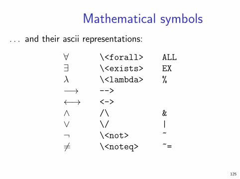
Mathematical symbols

. . . and their ascii representations:

∀ \<forall> ALL

∃ \<exists> EX

λ \<lambda> %

−→ -->

←→ <->

∧ /\ &

∨ \/ |

¬ \<not> ~

6= \<noteq> ~=

125

Sets over type ′a

′a set

• {}, {e1,. . . ,en}• e ∈ A, A ⊆ B• A ∪ B, A ∩ B, A − B, − A• . . .

∈ \<in> :

⊆ \<subseteq> <=

∪ \<union> Un

∩ \<inter> Int

126

Set comprehension

• {x. P} where x is a variable

• But not {t. P} where t is a proper term

• Instead: {t |x y z. P}is short for {v. ∃ x y z. v = t ∧ P}where x, y, z are the free variables in t

127

8 Logical Formulas

9 Proof Automation



128

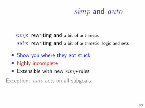
simp and auto

simp: rewriting and a bit of arithmetic

auto: rewriting and a bit of arithmetic, logic and sets

• Show you where they got stuck

• highly incomplete

• Extensible with new simp-rules

Exception: auto acts on all subgoals

129

fastforce

• rewriting, logic, sets, relations and a bit of arithmetic.

• incomplete but better than auto.

• Succeeds or fails

• Extensible with new simp-rules

130

blast

• A complete proof search procedure for FOL . . .

• . . . but (almost) without “=”

• Covers logic, sets and relations

• Succeeds or fails

• Extensible with new deduction rules

131

Automating arithmetic

arith:

• proves linear formulas (no “∗”)

• complete for quantifier-free real arithmetic

• complete for first-order theory of nat and int(Presburger arithmetic)

132

Sledgehammer

133

Architecture:

Isabelle

Goal& filtered library

↓ ↑ Proof

externalATPs1

Characteristics:

• Sometimes it works,

• sometimes it doesn’t.

Do you feel lucky?

1Automatic Theorem Provers134

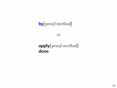
by(proof-method)

≈

apply(proof-method)done

135

Auto_Proof_Demo.thy

136

8 Logical Formulas

9 Proof Automation



137

Step-by-step proofs can be necessary if automation failsand you have to explore where and why it failed bytaking the goal apart.

138

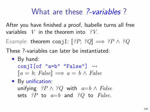
What are these ?-variables ?

After you have finished a proof, Isabelle turns all freevariables V in the theorem into ?V.

Example: theorem conjI: [[?P; ?Q]] =⇒ ?P ∧ ?Q

These ?-variables can later be instantiated:

• By hand:conjI[of "a=b" "False"] [[a = b; False]] =⇒ a = b ∧ False

• By unification:unifying ?P ∧ ?Q with a=b ∧ Falsesets ?P to a=b and ?Q to False.

139

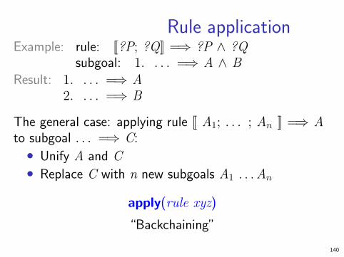
Rule applicationExample: rule: [[?P; ?Q]] =⇒ ?P ∧ ?Q

subgoal: 1. . . . =⇒ A ∧ BResult: 1. . . . =⇒ A

2. . . . =⇒ B

The general case: applying rule [[ A1; . . . ; An ]] =⇒ Ato subgoal . . . =⇒ C:• Unify A and C• Replace C with n new subgoals A1 . . .An

apply(rule xyz)

“Backchaining”

140

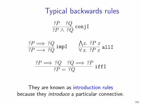
Typical backwards rules

?P ?Q?P ∧ ?Q

conjI

?P =⇒ ?Q?P −→ ?Q

impI

∧x. ?P x∀ x. ?P x

allI

?P =⇒ ?Q ?Q =⇒ ?P?P = ?Q

iffI

They are known as introduction rulesbecause they introduce a particular connective.

141

Automating intro rulesIf r is a theorem [[ A1; . . . ; An ]] =⇒ A then

(blast intro: r)

allows blast to backchain on r during proof search.

Example:

theorem le trans: [[ ?x ≤ ?y; ?y ≤ ?z ]] =⇒ ?x ≤ ?z

goal 1. [[ a ≤ b; b ≤ c; c ≤ d ]] =⇒ a ≤ d

proof apply(blast intro: le trans)

Also works for auto and fastforce

Can greatly increase the search space!

142

Forward proof: OF

If r is a theorem A =⇒ Band s is a theorem that unifies with A then

r[OF s]

is the theorem obtained by proving A with s.

Example: theorem refl: ?t = ?t

conjI[OF refl[of "a"]]

?Q =⇒ a = a ∧ ?Q

143

The general case:

If r is a theorem [[ A1; . . . ; An ]] =⇒ Aand r1, . . . , rm (m≤n) are theorems then

r[OF r1 . . . rm]

is the theorem obtainedby proving A1 . . . Am with r1 . . . rm.

Example: theorem refl: ?t = ?t

conjI[OF refl[of "a"] refl[of "b"]]

a = a ∧ b = b

144

From now on: ? mostly suppressed on slides

145

Single_Step_Demo.thy

146

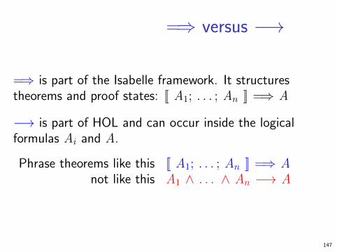
=⇒ versus −→

=⇒ is part of the Isabelle framework. It structurestheorems and proof states: [[ A1; . . . ; An ]] =⇒ A

−→ is part of HOL and can occur inside the logicalformulas Ai and A.

Phrase theorems like this [[ A1; . . . ; An ]] =⇒ Anot like this A1 ∧ . . . ∧ An −→ A

147

8 Logical Formulas

9 Proof Automation



148

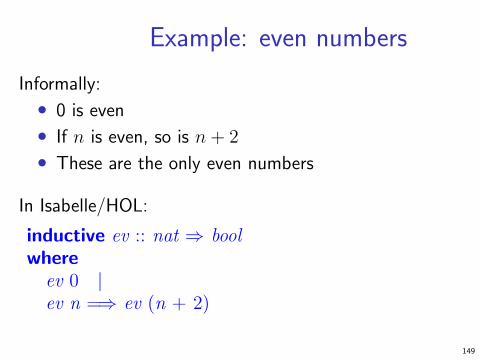
Example: even numbers

Informally:

• 0 is even

• If n is even, so is n+ 2

• These are the only even numbers

In Isabelle/HOL:

inductive ev :: nat ⇒ boolwhereev 0 |ev n =⇒ ev (n + 2)

149

An easy proof: ev 4

ev 0 =⇒ ev 2 =⇒ ev 4

150

Consider

fun evn :: nat ⇒ bool whereevn 0 = True |evn (Suc 0) = False |evn (Suc (Suc n)) = evn n

A trickier proof: ev m =⇒ evn m

By induction on the structure of the derivation of ev m

Two cases: ev m is proved by

• rule ev 0=⇒ m = 0 =⇒ evn m = True

• rule ev n =⇒ ev (n+2)=⇒ m = n+2 and evn n (IH)=⇒ evn m = evn (n+2) = evn n = True

151

Rule induction for evTo prove

ev n =⇒ P n

by rule induction on ev n we must prove

• P 0

• P n =⇒ P(n+2)

Rule ev.induct:

ev n P 0∧n. [[ ev n; P n ]] =⇒ P(n+2)

P n

152

Format of inductive definitions

inductive I :: τ ⇒ bool where[[ I a1; . . . ; I an ]] =⇒ I a |...

Note:

• I may have multiple arguments.

• Each rule may also contain side conditions notinvolving I.

153

Rule induction in general

To prove

I x =⇒ P x

by rule induction on I xwe must prove for every rule

[[ I a1; . . . ; I an ]] =⇒ I a

that P is preserved:

[[ I a1; P a1; . . . ; I an; P an ]] =⇒ P a

154

!Rule induction is absolutely central

to (operational) semanticsand the rest of this lecture course

!

155

Inductive_Demo.thy

156

Inductively defined sets

inductive_set I :: τ set where[[ a1 ∈ I; . . . ; an ∈ I ]] =⇒ a ∈ I |...

Difference to inductive:

• arguments of I are tupled, not curried

• I can later be used with set theoretic operators,eg I ∪ . . .

157

Chapter 5

Isar: A Language forStructured Proofs

158

12 Isar by example

13 Proof patterns

14 Streamlining Proofs

15 Proof by Cases and Induction

159

Apply scripts

• unreadable

• hard to maintain

• do not scale

No structure!

160

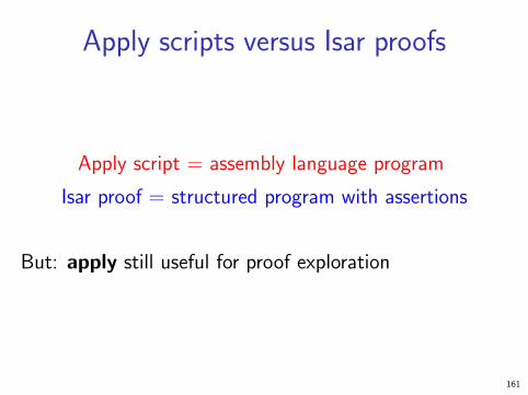
Apply scripts versus Isar proofs

Apply script = assembly language program

Isar proof = structured program with assertions

But: apply still useful for proof exploration

161

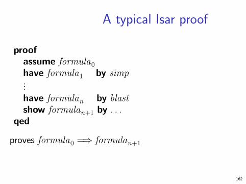
A typical Isar proof

proofassume formula0

have formula1 by simp...have formulan by blastshow formulan+1 by . . .

qed

proves formula0 =⇒ formulan+1

162

Isar core syntaxproof = proof [method] step∗ qed

| by method

method = (simp . . . ) | (blast . . . ) | (induction . . . ) | . . .

step = fix variables (∧

)| assume prop (=⇒)| [from fact+] (have | show) prop proof

prop = [name:] ”formula”

fact = name | . . .

163

12 Isar by example

13 Proof patterns



164

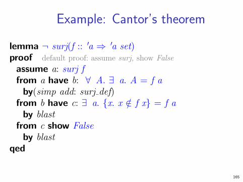
Example: Cantor’s theorem

lemma ¬ surj(f :: ′a ⇒ ′a set)proof default proof: assume surj, show False

assume a: surj ffrom a have b: ∀ A. ∃ a. A = f a

by(simp add: surj def)from b have c: ∃ a. {x. x /∈ f x} = f a

by blastfrom c show False

by blastqed

165

Isar_Demo.thy

Cantor and abbreviations

166

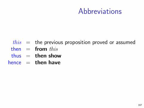
Abbreviations

this = the previous proposition proved or assumedthen = from thisthus = then show

hence = then have

167

using and with

(have|show) prop using facts=

from facts (have|show) prop

with facts=

from facts this

168

Structured lemma statement

lemmafixes f :: ′a ⇒ ′a setassumes s: surj fshows False

proof − no automatic proof step

have ∃ a. {x. x /∈ f x} = f a using sby(auto simp: surj def)

thus False by blastqed

Proves surj f =⇒ Falsebut surj f becomes local fact s in proof.

169

The essence of structured proofs

Assumptions and intermediate factscan be named and referred to explicitly and selectively

170

Structured lemma statements

fixes x :: τ1 and y :: τ2 . . .assumes a: P and b: Q . . .shows R

• fixes and assumes sections optional

• shows optional if no fixes and assumes

171

12 Isar by example

13 Proof patterns



172

Case distinction

show Rproof cases

assume P...show R 〈proof 〉

nextassume ¬ P...show R 〈proof 〉

qed

have P ∨ Q 〈proof 〉then show Rproof

assume P...show R 〈proof 〉

nextassume Q...show R 〈proof 〉

qed

173

Contradiction

show ¬ Pproof

assume P...show False 〈proof 〉

qed

show Pproof (rule ccontr)

assume ¬P...show False 〈proof 〉

qed

174

←→

show P ←→ Qproof

assume P...show Q 〈proof 〉

nextassume Q...show P 〈proof 〉

qed

175

∀ and ∃ introduction

show ∀ x. P(x)proof

fix x local fixed variable

show P(x) 〈proof 〉qed

show ∃ x. P(x)proof...show P(witness) 〈proof 〉

qed

176

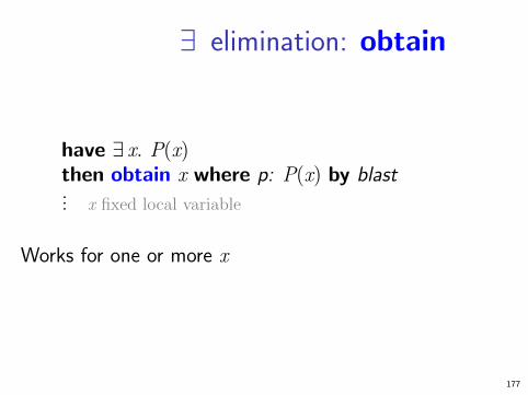
∃ elimination: obtain

have ∃ x. P(x)then obtain x where p: P(x) by blast... x fixed local variable

Works for one or more x

177

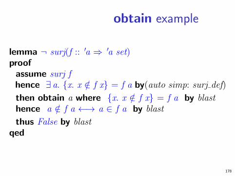
obtain example

lemma ¬ surj(f :: ′a ⇒ ′a set)proof

assume surj fhence ∃ a. {x. x /∈ f x} = f a by(auto simp: surj def)

then obtain a where {x. x /∈ f x} = f a by blasthence a /∈ f a ←→ a ∈ f a by blast

thus False by blastqed

178

Set equality and subset

show A = Bproof

show A ⊆ B 〈proof 〉next

show B ⊆ A 〈proof 〉qed

show A ⊆ Bproof

fix xassume x ∈ A...show x ∈ B 〈proof 〉

qed

179

Isar_Demo.thy

Exercise

180

12 Isar by example

13 Proof patterns



181

14 Streamlining ProofsPattern Matching and QuotationsTop down proof developmentmoreoverLocal lemmas

182

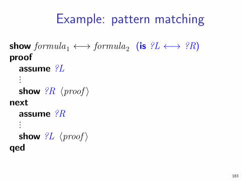
Example: pattern matching

show formula1 ←→ formula2 (is ?L ←→ ?R)proof

assume ?L...show ?R 〈proof 〉

nextassume ?R...show ?L 〈proof 〉

qed

183

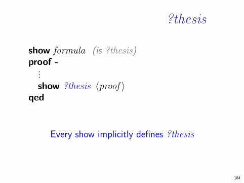
?thesis

show formula (is ?thesis)proof -

...show ?thesis 〈proof 〉

qed

Every show implicitly defines ?thesis

184

let

Introducing local abbreviations in proofs:

let ?t = "some-big-term"...have ". . . ?t . . . "

185

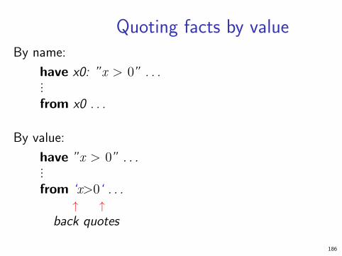
Quoting facts by valueBy name:

have x0: ”x > 0” . . ....from x0 . . .

By value:

have ”x > 0” . . ....from ‘x>0‘ . . .

↑ ↑back quotes

186

Isar_Demo.thy

Pattern matching and quotations

187


188

Example

lemma∃ ys zs. xs = ys @ zs ∧(length ys = length zs ∨ length ys = length zs + 1)

proof ???

189

Isar_Demo.thy

Top down proof development

190

When automation failsSplit proof up into smaller steps.

Or explore by apply:

have . . . using . . .apply - to make incoming facts

part of proof stateapply auto or whateverapply . . .

At the end:

• done

• Better: convert to structured proof191


192

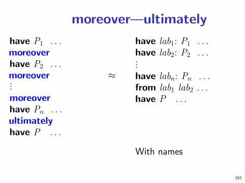
moreover—ultimately

have P1 . . .moreoverhave P2 . . .moreover...moreoverhave Pn . . .ultimatelyhave P . . .

≈

have lab1: P1 . . .have lab2: P2 . . ....have labn: Pn . . .from lab1 lab2 . . .have P . . .

With names

193


194

Local lemmas

have B if name: A1 . . . Am for x1 . . . xn〈proof 〉

proves [[ A1; . . . ; Am ]] =⇒ Bwhere all xi have been replaced by ?xi.

195

Proof state and Isar text

In general: proof method

Applies method and generates subgoal(s):∧x1 . . . xn. [[ A1; . . . ; Am ]] =⇒ B

How to prove each subgoal:

fix x1 . . . xnassume A1 . . . Am...show B

Separated by next

196

12 Isar by example

13 Proof patterns



197

Isar_Induction_Demo.thy

Proof by cases

198

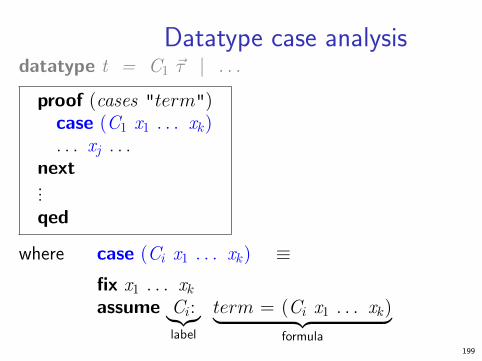
Datatype case analysisdatatype t = C1 ~τ | . . .

proof (cases "term")case (C1 x1 . . . xk). . . xj . . .

next...qed

where case (Ci x1 . . . xk) ≡fix x1 . . . xkassume Ci:︸︷︷︸

label

term = (Ci x1 . . . xk)︸︷︷︸formula

199


Structural induction for nat

200

Structural induction for nat

show P(n)proof (induction n)

case 0 ≡ let ?case = P (0)...show ?case

nextcase (Suc n) ≡ fix n assume Suc: P (n)... let ?case = P (Suc n)...show ?case

qed

201

Structural induction with =⇒show A(n) =⇒ P(n)proof (induction n)

case 0 ≡ assume 0: A(0)... let ?case = P(0)show ?case

nextcase (Suc n) ≡ fix n... assume Suc: A(n) =⇒ P(n)

A(Suc n)... let ?case = P(Suc n)show ?case

qed

202

Named assumptions

In a proof of

A1 =⇒ . . . =⇒ An =⇒ B

by structural induction:

In the context ofcase C

we have

C.IH the induction hypotheses

C.prems the premises Ai

C C.IH + C.prems

203

A remark on style

• case (Suc n) . . . show ?caseis easy to write and maintain

• fix n assume formula . . . show formula ′

is easier to read:• all information is shown locally• no contextual references (e.g. ?case)

204

15 Proof by Cases and InductionRule InductionRule Inversion

205


Rule induction

206

Rule induction

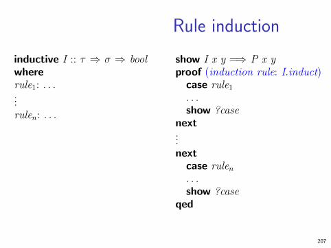
inductive I :: τ ⇒ σ ⇒ boolwhererule1: . . ....rulen: . . .

show I x y =⇒ P x yproof (induction rule: I.induct)

case rule1. . .show ?case

next...next

case rulen. . .show ?case

qed

207

Fixing your own variable names

case (rulei x1 . . . xk)

Renames the first k variables in rulei (from left to right)to x1 . . . xk.

208

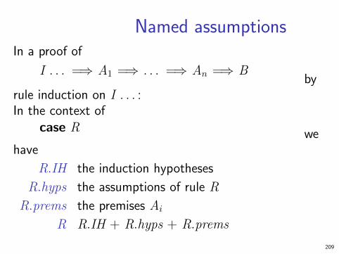
Named assumptionsIn a proof of

I . . . =⇒ A1 =⇒ . . . =⇒ An =⇒ Bby

rule induction on I . . . :In the context of

case R wehave

R.IH the induction hypotheses

R.hyps the assumptions of rule R

R.prems the premises Ai

R R.IH + R.hyps + R.prems

209

15 Proof by Cases and InductionRule InductionRule Inversion

210

Rule inversion

inductive ev :: nat ⇒ bool whereev0: ev 0 |evSS: ev n =⇒ ev(Suc(Suc n))

What can we deduce from ev n ?That it was proved by either ev0 or evSS !

ev n =⇒ n = 0 ∨ (∃ k. n = Suc (Suc k) ∧ ev k)

Rule inversion = case distinction over rules

211


Rule inversion

212

Rule inversion templatefrom ‘ev n‘ have Pproof cases

case ev0 n = 0...show ?thesis . . .

nextcase (evSS k) n = Suc (Suc k), ev k...show ?thesis . . .

qed

Impossible cases disappear automatically

213

Documents

Concrete Semanticsconcrete-semantics.org/slides-isabelle.pdf · 2019-10-14 · Why Semantics? Without semantics, we do not really know what our programs mean. We merely have a good