Conditional Credences - Fitelson

Chapter 3

Conditional Credences

Chapter 2’s discussion was confined to unconditional credence, an agent’soutright degree of confidence that a particular proposition is true. Thischapter takes up conditional credence, an agent’s credence that one propo-sition is true on the supposition that another is.

The main focus of this chapter is our fourth core Bayesian rule: theRatio Formula. This rational constraint on conditional credences has anumber of important consequences, including Bayes’ Theorem (which givesBayesianism its name).

Conditional credences are also central to the way Bayesians understandevidential relevance. I will define relevance as positive correlation, thenexplain how this notion has been used to investigate causal relations throughthe concept of screening off.

Having achieved a deeper understanding of the mathematics of condi-tional credences, I return at the end of the chapter to what exactly a condi-tional credence is. In particular, I discuss an argument by David Lewis thata conditional credence can’t be understood as an unconditional credence ina conditional.

3.1 Conditional credences and the Ratio Formula

Andy and Bob know that two events will occur simultaneously in separaterooms: a fair coin will be flipped, and a clairvoyant will predict how it willland. Let H represent the proposition that the coin comes up heads, andC represent the proposition that the clairvoyant predicts heads. SupposeAndy and Bob each assign an unconditional credence of 1{2 to H and anunconditional credence of 1{2 to C.

51

52 CHAPTER 3. CONDITIONAL CREDENCES

Although Andy and Bob assign the same unconditional credences aseach other to H and C, they still might take these propositions to be relatedin different ways. We could tease tease out those differences by saying toeach agent, “I have no idea how the coin is going to come up or whatthe clairvoyant is going to say. But suppose for a moment the clairvoyantpredicts heads. On this supposition, how confident are you that the coinwill come up heads?” If Andy says 1{2 and Bob says 99{100, that’s a goodindication that Bob has more faith in the mystical than Andy.

The quoted question in the previous paragraph elicits Andy and Bob’sconditional credences, as opposed to the unconditional credences discussedin Chapter 2. An unconditional credence is a degree of belief assigned to asingle proposition, indicating how confident the agent is that that proposi-tion is true. A conditional credence is a degree of belief assigned to anordered pair of propositions, indicating how confident the agent is that thefirst proposition is true on the supposition that the second is. We symbolizeconditional credences as follows:

crpH |Cq “ 1{2 (3.1)

This equation says that a particular agent (in this case, Andy) has a 1{2credence that the coin comes up heads conditional on the supposition thatthe clairvoyant predicts heads. The vertical bar indicates a conditional cre-dence; to the right of the bar is the proposition supposed; to the left of thebar is the proposition evaluated in light of that supposition. The propositionto the right of the bar is sometimes called the condition; I am not awareof any generally-accepted name for the proposition on the left.

Note that a conditional credence is assigned to an ordered pair of propo-sitions. It makes a difference which proposition is supposed and which isevaluated. Consider a case in which I’m going to roll a fair die and you havevarious credences involving the proposition E that it comes up even and theproposition 6 that it comes up six. Compare:

crp6 |Eq “ 1{3 (3.2)

crpE | 6q “ 1 (3.3)

3.1.1 The Ratio Formula

Section 2.2 described Kolmogorov’s probability axioms, which Bayesianstake to represent rational constraints on an agent’s unconditional credences.Bayesians then add a constraint relating conditional to unconditional cre-dences:

3.1. CONDITIONAL CREDENCES AND THE RATIO FORMULA 53

Figure 3.1: crpP |Qq

P

Q

Ratio Formula: For any P and Q in L, if crpQq ą 0 then

crpP |Qq “crpP & Qq

crpQq

Stated this way, the Ratio Formula remains silent on the value of crpP |Qqwhen crpQq “ 0. There are various positions on how one should assignconditional credences when the condition has credence 0; we’ll cover someof them in our discussion of the infinite in Chapter 5.

Why should an agent’s conditional credences equal the ratio of thoseunconditionals? Consider Figure 3.1. The rectangle represents all the pos-sible worlds the agent entertains. The agent’s unconditional credence in Pis the fraction of that rectangle taken up by the P -circle. (The area of therectangle is stipulated to be 1, so that fraction is the area of the P -circledivided by 1, which is just the area of the P -circle.) When we ask the agentto evaluate a credence conditional on the supposition that Q, she temporar-ily narrows her focus to just those possibilities that make Q true. In otherwords, she excludes from her attention the worlds I’ve shaded in the dia-gram, and considers only what’s in the Q-circle. The agent’s credence in Pconditional on Q is the fraction of the Q-circle occupied by P -worlds. Soit’s the area of the PQ overlap divided by the area of the entire Q-circle,which is crpP & Qq{crpQq.

In the scenario in which I roll a fair die, your initial doxastic possibilitiesinclude all six outcomes of the die roll. If I ask you to evaluate crp6 |Eq,you exclude from consideration all the odd outcomes. That doesn’t meanyou’ve actually learned that the die outcome is even; I’ve just asked youto suppose momentarily that it comes up even and assign a confidence to


other propositions in light of that supposition. You distribute your credenceequally over the outcomes that remain under consideration (2, 4, and 6), soyour credence in 6 conditional on even is 1{3.

We get the same result from the Ratio Formula:

crp6 |Eq “crp6 & Eq

crpEq“

1{6

1{2“

1

3(3.4)

The Ratio Formula allows us to calculate your conditional credences (confi-dences under a supposition) in terms of your unconditional credences (con-fidences assigned when no suppositions are made). Hopefully it’s obviouswhy E gets an unconditional credence of 1{2 in this case; as for 6&E, that’sequivalent to just 6, so it gets an unconditional credence of 1{6.1

Warning: Mathematicians often take the Ratio Formula to be adefinition of conditional probability. From their point of view, aconditional probability has the value it does in virtue of two uncon-ditional probabilities’ standing in a certain ratio. But I do not wantto reduce the possession of a conditional credence to the possessionof two unconditional credences standing in a particular relation. Itake a conditional credence to be a genuine mental state (an attitudetowards an ordered pair of propositions) capable of being elicited invarious ways, such as by asking an agent her confidence in a proposi-tion given a supposition. The Ratio Formula is a rational constrainton how an agent’s conditional credences should relate to her un-conditional credences, and as a normative constraint (rather than adefinition) it can be violated—by assigning a conditional credencethat doesn’t equal the specified ratio.

The point of the previous warning is that the Ratio Formula is a rationalconstraint, and not all agents meet all the rational constraints on theircredences. Yet for an agent who does satisfy the Ratio Formula, there canbe no difference in her conditional credences without a difference in herunconditional credences as well. (We say that a rational agent’s conditionalcredences supervene on her unconditional credences.) Fully specifying anagent’s unconditional credence distribution suffices to specify her conditionalcredences as well. For instance, we might specify Andy’s and Bob’s credencedistributions using the following stochastic truth-table:


C H crA crBT T 1{4 99{200

T F 1{4 1{200

F T 1{4 1{200

F F 1{4 99{200

Here crA represents Andy’s credences and crB represents Bob’s. Andy’sunconditional credence in C is identical to Bob’s—the values on the firsttwo rows sum to 1{2 for each of them. Similarly, Andy and Bob have thesame unconditional credence in H (the sum of the first and third rows).Yet Andy and Bob disagree in their confidence that the coin will come upheads given that the clairvoyant predicts heads. Using the Ratio Formula,we calculate this conditional credence by dividing the value on the first rowof the table by the sum of the values on the first two rows. This yields:

crApH |Cq “1{4

1{2“

1

2‰

99

100“

99{200

100{200“ crBpH |Cq (3.5)

Bob has high confidence in the clairvoyant’s abilities. So on the suppositionthat the clairvoyant predicts heads, Bob is almost certain that heads willcome up on the flip. Andy, on the other hand, is skeptical, so supposingthat the clairvoyant predicts heads leaves his opinions about the flip outcomeunchanged.

3.1.2 Consequences of the Ratio Formula

Combining the Ratio Formula with the probability axioms yields furtheruseful probability rules. First we have the

Law of Total Probability: For any finite partition Q1, Q2, . . . , Qn in L,

crpP q “ crpP |Q1q ¨ crpQ1q ` crpP |Q2q ¨ crpQ2q`

. . .` crpP |Qnq ¨ crpQnq

Suppose you’re trying to predict whether I will bike to work tomorrow,but you’re unsure if the weather will rain, hail, or be clear. The Law ofTotal Probability allows you to systematically work through the possibilitiesin that partition. You multiply your confidence that it will rain by yourconfidence that I’ll bike should it rain. Then you multiply your confidencethat it’ll hail by your confidence in my biking given hail. Finally you multiplyyour unconditional credence that it’ll be clear by your conditional credencethat I’ll bike given that it’s clear. Adding these three products together gives


your unconditional credence that I’ll bike. (In the formula the propositionthat I’ll bike plays the role of P and the three weather possibilities are Q1,Q2, and Q3.)

Next, the Ratio Formula makes any conditional credence distributionitself a probability distribution. To understand what that means and howit works in general, we’ll start with a very special example. Let’s say I askyou to report your unconditional credences in some propositions. Then I askyou to assign credences to those propositions conditional on the suppositionof. . . nothing. I give you nothing more to suppose. Clearly you’ll just reportback to me the same credences. Bayesians represent vacuous informationas a tautology, so what we’ve just seen is that a rational agent’s credencesconditional on a tautology equal her unconditional credences.2 In otherwords, for any P in L

crpP |Tq “ crpP q (3.6)

Since we’re assuming the agent’s unconditional credences satisfy theprobability axioms, the credences that result if we ask her to suppose a tau-tology also satisfy the probability axioms. The distribution crp¨ |Tq (wherethe “¨” is a blank to be filled by a proposition) must be a probability distri-bution. Remarkably, this turns out to be true for non-tautologous conditionsas well. Pick any proposition R in L such that crpRq ą 0, and the functionyou get by taking various credences conditional on the supposition of R willsatisfy the probability axioms. That is,

• For any proposition P in L, crpP |Rq ě 0.

• For any tautology T in L, crpT |Rq “ 1.

• For any mutually exclusive propositions P and Q in L,crpP _Q |Rq “ crpP |Rq ` crpQ |Rq.

In other words, crp¨ |Rq satisfies Kolmogorov’s probability axioms. (You’llprove this in Exercise 3.3.)

Knowing that a conditional credence distribution is a probability dis-tribution can be a handy shortcut. (It also has a significance for updat-ing credences that we’ll discuss in Chapter 4.) Because it’s a probabilitydistribution, a conditional credence distribution must satisfy all the conse-quences of the probability axioms we saw in Section 2.2.1. If I tell you thatcrpP |Rq “ 0.7, you know that crp„P |Rq “ 0.3, by the following implemen-tation of the Negation rule:

crp„P |Rq “ 1´ crpP |Rq (3.7)

Similarly, by Entailment if P ( Q then crpP |Rq ď crpQ |Rq.


3.1.3 Bayes’ Theorem

The most famous consequence of the Ratio Formula and Kolmogorov’s ax-ioms is

Bayes’ Theorem: For any H and E in L,

crpH |Eq “crpE |Hq ¨ crpHq

crpEq

The first thing to say about Bayes’ Theorem is that it is a theorem—it canbe proven straightforwardly from the axioms and Ratio Formula. This isworth remembering, because there is a great deal of controversy about howBayesians apply the theorem. (The significance they attach to this theoremis how Bayesians came to be called “Bayesians”.)

What philosophical significance could attach to an equation that is, inthe end, just a truth of mathematics? The theorem was first articulated bythe Reverend Thomas Bayes in the 1700s.3 Prior to Bayes, much of prob-ability theory was concerned with problems of direct inference. Directinference starts with the supposition of some probabilistic hypothesis, thenasks how likely that hypothesis makes a particular experimental result. Youprobably learned to solve many direct inference problems in school, such as“Suppose I flip a fair coin 20 times; how likely am I to get exactly 19 heads?”Here the probabilistic hypothesis H is that the coin is fair, and the exper-imental result E is exactly 19 heads. Your credence that the experimentalresult will occur on the supposition that the hypothesis is true—crpE |Hq—is called the likelihood.4

Yet Bayes was also interested in inverse inference. Instead of makingsuppositions about hypotheses and determining probabilities of courses ofevidence, his theorem allows us to calculate probabilities of hypotheses fromsuppositions about evidence. Instead of calculating the likelihood crpE |Hq,Bayes’ Theorem shows us how to calculate crpH |Eq. A problem of inverseinference might ask, “Suppose a coin comes up heads on exactly 19 of 20flips; how probable is it that the coin is fair?”

Assessing the significance of Bayes’ Theorem, Hans Reichenbach wrote,

The method of indirect evidence, as this form of inquiry is called,consists of inferences that on closer analysis can be shown tofollow the structure of the rule of Bayes. The physician’s infer-ences, leading from the observed symptoms to the diagnosis ofa specified disease, are of this type; so are the inferences of thehistorian determining the historical events that must be assumed


for the explanation of recorded observations; and, likewise, theinferences of the detective concluding criminal actions from in-conspicuous observable data. . . . Similarly, the general inductiveinference from observational data to the validity of a given scien-tific theory must be regarded as an inference in terms of Bayes’rule. (Reichenbach 1935/1949, pp. 94–5)5

Here’s an example of inverse inference: You’re a biologist studying aparticular species of fish, and you want to know whether the genetic allelecoding for blue fins is dominant or recessive. Intially you assign 50-50 cre-dence to each possibility. A simple direct inverse from the theory of geneticstells you that if the allele is dominant, roughly 3 out of 4 species memberswill have blue fins; if the allele is recessive blue fins will appear on roughly25% of the fish. But you’re going to perform an inverse inference, mak-ing experimental observations to decide between genetic hypotheses. Youwill capture fish from the species at random and examine their fins. Howsignificant will your first observation be to your credences in dominant vs.recessive? When you contemplate various ways that observation might turnout, how should supposing one outcome or the other affect your credencesabout the allele? Before we do the calculation, try estimating how confidentyou should be that the allele is dominant on the supposition that the firstfish you observe has blue fins.

In this example our hypothesis H will be that the blue-fin allele is dom-inant. The evidence E to be supposed is that a randomly-drawn fish hasblue fins. We want to calculate the posterior value crpH |Eq. This valueis called the “posterior” because it’s your credence in the hypothesis H af-ter the evidence E has been supposed. In order to calculate this posterior,Bayes’ Theorem requires the values of crpE |Hq, crpHq, and crpEq.

crpE |Hq is the likelihood of drawing a blue-finned fish on the hypothesisthat the allele is dominant. On the supposition that the allele is dominant,75% of the fish have blue fins, so your crpE |Hq value should be 0.75. Theother two values are known as priors; they are your unconditional credencesin the hypothesis and the evidence before anything is supposed. The priorin the hypothesis H is easy—we said you initially split your credence 50-50between dominant and recessive. So crpHq is 0.5. But what about the priorin the evidence? How confident are you before observing any fish that thefirst one you draw will have blue fins?

Here we can apply the Law of Total Probability to the partition consist-ing of H and „H. This yields:

crpEq “ crpE |Hq ¨ crpHq ` crpE | „Hq ¨ crp„Hq (3.8)


The values on the righthand side are all either priors in the hypothesis orlikelihoods. These values we can easily calculate. So

crpEq “ 0.75 ¨ 0.5` 0.25 ¨ 0.5 “ 0.5 (3.9)

Plugging all these values into Bayes’ Theorem gives us


crpEq“

0.75 ¨ 0.5

0.5“ 0.75 (3.10)

Observing a single fish has the potential to change your credences sub-stantially. On the supposition that the fish you draw has blue fins, yourcredence that the blue-fin allele is dominant goes from its prior value of 1{2to a posterior of 3{4.

Again, all of this is strictly mathematics from a set of axioms that arerarely disputed. So why has Bayes’ Theorem been the focus of controversy?One issue is the role Bayesians see the theorem playing in updating our atti-tudes over time; we’ll return to that application of the theorem in Chapter4. But the main idea that Bayesians take from Bayes—and that has provencontroversial—is that probabilistic inverse inference is the key to induction.Bayesians think the primary way we ought to draw conclusions from data—how we ought to reason about scientific hypotheses, say, on the basis ofexperimental evidence—is by calculating posterior credences using Bayes’Theorem. This view stands in direct conflict with other statistical methods,such as frequentism and likelihoodism. Once we have considerably deepenedour understanding of Bayesian Epistemology, we will discuss this conflict inChapter XXX.

Before moving on, I’d like to highlight two useful alternative forms ofBayes’ Theorem. We’ve just seen that calculating the prior of the evidence—crpEq—can be easier if we break it up using the Law of Total Probability.Incorporating that manuever into Bayes’ Theorem yields


crpE |Hq ¨ crpHq ` crpE | „Hq ¨ crp„Hq(3.11)

When a particular hypothesis H is under consideration, its negation „H isknown as the catchall hypothesis. So this form of Bayes’ Theorem calcu-lates the posterior in the hypothesis from the priors and likelihoods of thehypothesis and its catchall.

In other situations we have multiple hypotheses under consideration in-stead of just one. Given a finite partition of n hypotheses H1, H2, . . . ,Hn,


the Law of Total Probability transforms the denominator of Bayes’ Theoremto yield

crpHi |Eq “crpE |Hiq ¨ crpHiq

crpE |H1q ¨ crpH1q ` crpE |H2q ¨ crpH2q ` . . .` crpE |Hnq ¨ crpHnq

(3.12)This version allows you to calculate the posterior of one particular hypothesisHi in the partition from the priors and likelihoods of all the hypotheses.

3.2 Relevance and independence

Andy doesn’t believe in hocus pocus; from his point of view, informationabout what a clairvoyant predicts is irrelevant to determining how a coinflip will come out. So supposing that a clairvoyant predicts heads makes nodifference to Andy’s confidence in a heads outcome. If C says the clairvoyantpredicts heads, H says the coin lands heads, and crA is Andy’s credencedistribution, we have

crApH |Cq “ 1{2 “ crApHq (3.13)

Generalizing this idea yields a key definition: Proposition P is proba-bilistically independent of proposition Q relative to distribution cr justin case

crpP |Qq “ crpP q (3.14)

In this case Bayesians also say that Q is irrelevant to P . When Q isirrelevant to P , supposing Q leaves an agent’s credence in P unchanged.

Notice that probabilistic independence is always relative to a credencedistribution cr. The very same propositions P and Q might be independentrelative to one credence distribution but dependent relative to another. (Rel-ative to Andy’s credences the clairvoyant’s prediction is irrelevant to the flipoutcome, but relative to the credences of his friend Bob—who believes inpsychic powers—it is not.) In what follows I may omit reference to a par-ticular credence function when context makes it clear, but you should keepthe relativity of independence to probability distribution in the back of yourmind.

While Equation (3.14) will be our official definition of probabilistic in-dependence, there are many equivalent tests for independence. Given theprobability axioms and Ratio Formula, the following equations are all true

3.2. RELEVANCE AND INDEPENDENCE 61

just when Equation (3.14) is:6

crpP q “ crpP | „Qq (3.15)

crpP |Qq “ crpP | „Qq (3.16)

crpQ |P q “ crpQq “ crpQ | „P q (3.17)

crpP & Qq “ crpP q ¨ crpQq (3.18)

The equivalence of Equations (3.14) and (3.15) tells us that if supposingQ makes no difference to an agent’s confidence in P , then supposing „Qmakes no difference as well. The equivalence of (3.14) and (3.17) showsus that independence is symmetric: if supposing Q makes no difference toan agent’s credence in P , supposing P won’t change the agent’s attitudetowards Q either. Finally, Equation (3.18) embodies a useful probabilityrule:

Multiplication: P and Q are probabilistically independent relative to crif and only if crpP & Qq “ crpP q ¨ crpQq.

(Some authors define probabilistic independence using this biconditional,but we will define independence using Equation (3.14) and then treat Mul-tiplication as a consequence.)

Notice that we can calculate the credence of a conjunction by multiplyingthe credences of its conjuncts only when those conjuncts are independent.This trick will not work for any arbitrary propositions. The general formulafor credence in a conjunction can be derived quickly from the Ratio Formula:

crpP & Qq “ crpP |Qq ¨ crpQq (3.19)

When P and Q are probabilistically independent, the first term on the right-hand side equals crpP q.

It’s important not to get Multiplication and Finite Additivity confused.Finite Additivity says that the credence of a disjunction is the sum of thecredences of its mutually exclusive disjuncts. Multiplication says that thecredence of a conjunction is the product of the credences of its independentconjuncts. If I flip two fair coins in succession, heads on the first and headson the second are independent, while heads on the first and tails on the firstare mutually exclusive.

Probabilistic independence fails to hold when one proposition is relevantto the other. Replace the ““” signs in Equations (3.14) through (3.18) with“ą” signs and you have tests for Q’s being positively relevant to P . Oncemore the tests are equivalent—if any of the resulting inequalities is true, all


of them are. Q is positively relevant to P when assuming Q makes you moreconfident in P . For example, since Bob believes in mysticism he takes theclairvoyant’s predictions to be highly relevant to the outcome of the coinflip—supposing that the clairvoyant has predicted heads takes him fromequanimity to near-certainty in a heads outcome. Bob assigns

crBpH |Cq “ 99{100 ą 1{2 “ crBpHq (3.20)

Like independence, positive relevance is symmetric. Given his high confi-dence in the clairvoyant’s accuracy, supposing that the coin came up headswill make Bob highly confident that the clairvoyant predicted it would.

Similarly, replacing the ““” signs with “ă” signs above yields tests fornegative relevance. For Bob, the clairvoyant’s predicting heads is nega-tively relevant to the coin’s coming up tails. Like positive correlation, nega-tive correlation is symmetric (supposing a tails outcome makes Bob less con-fident in a heads prediction). “Relevance” terms have a number of synonyms.Instead of finding “positively/negatively relevant” terminology, you’ll some-times find “positively/negatively dependent”, “positively/negatively corre-lated”, or even “correlated/anti-correlated” used.

The strongest forms of positive and negative relevance are entailmentand refutation. Suppose a hypothesis H has nonextreme prior credence.If a particular piece of evidence E entails the hypothesis, the probabilityaxioms and Ratio Formula tell us

crpH |Eq “ 1 (3.21)

Supposing E takes H from a middling credence to the highest credenceallowed. Similarly, if E refutes H (what philosophers of science call falsifi-cation), then

crpH |Eq “ 0 (3.22)

Relevance will be most important to us because of its connection toconfirmation, the Bayesian notion of evidential support. A piece of evidenceconfirms a hypothesis only if it’s relevant to that hypothesis. Put anotherway, learning a piece of evidence changes a rational agent’s credence in ahypothesis only if that evidence is relevant to the hypothesis. (Much moreon all this later.)

3.2.1 Conditional independence and screening off

The definition of probabilistic independence compares an agent’s conditionalcredence in a proposition to her unconditional credence in that proposition.


But we can also compare conditional credences. When Bob, who believesin the occult, hears a clairvoyant’s prediction about the outcome of a faircoin flip, he takes it to be highly correlated with the true flip outcome.But what if we ask Bob to suppose that this particular clairvoyant is animpostor? Once he supposes the clairvoyant is an impostor, Bob may seethe clairvoyant’s predictions as completely irrelevant to the flip outcome.Let C be the proposition that the clairvoyant predicts heads, H be theproposition that the coin comes up heads, and I be the proposition that theclairvoyant is an impostor. It’s possible for Bob’s credences to satisfy bothof the following equations at once:

crpH |Cq ą crpHq (3.23)

crpH |C & Iq “ crpH | Iq (3.24)

Equation (3.23) tells us that unconditionally, Bob takes C to be relevant toH. But conditional on the supposition of I, C becomes independent of H;supposing C & I gives Bob the same confidence in H as supposing I alone.

Generalizing this idea yields the following definition of conditional in-dependence: P is probabilistically independent of Q conditional on R justin case

crpP |Q & Rq “ crpP |Rq (3.25)

If this equality fails to hold, we say that P is relevant to (or dependent on)Q conditional on R.

One more piece of terminology: We will say that R screens off P fromQ when P is unconditionally dependent on Q but independent of Q condi-tional on R. In other words, supposing R makes the correlation between Pand Q disappear. Equations (3.23) and (3.24) demonstrate that for Bob,I screens off H from C.7 We’ll now consider a number of challenging andpuzzling probabilistic phenomena whose explanations involve the notions ofconditional dependence and screening off.

3.2.2 The Gambler’s Fallacy

People often act as if future chancy events will “compensate” for unexpectedpast results. When a good hitter strikes out many times in a row, someonewill say he’s “due” for a hit. If a fair coin comes up heads 19 times in a row,many people become more confident that the next outcome will be tails.

This mistake is known as the Gambler’s Fallacy.8 A person who makesthe mistake is thinking along something like the following lines: In twentyflips of a fair coin, it’s more probable to get 19 heads and 1 tail than it is to


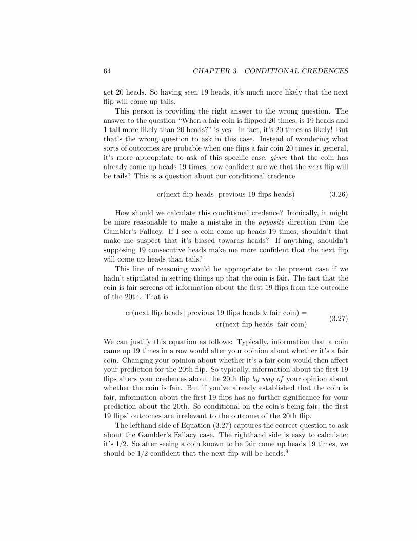
get 20 heads. So having seen 19 heads, it’s much more likely that the nextflip will come up tails.

This person is providing the right answer to the wrong question. Theanswer to the question “When a fair coin is flipped 20 times, is 19 heads and1 tail more likely than 20 heads?” is yes—in fact, it’s 20 times as likely! Butthat’s the wrong question to ask in this case. Instead of wondering whatsorts of outcomes are probable when one flips a fair coin 20 times in general,it’s more appropriate to ask of this specific case: given that the coin hasalready come up heads 19 times, how confident are we that the next flip willbe tails? This is a question about our conditional credence

crpnext flip heads |previous 19 flips headsq (3.26)

How should we calculate this conditional credence? Ironically, it mightbe more reasonable to make a mistake in the opposite direction from theGambler’s Fallacy. If I see a coin come up heads 19 times, shouldn’t thatmake me suspect that it’s biased towards heads? If anything, shouldn’tsupposing 19 consecutive heads make me more confident that the next flipwill come up heads than tails?

This line of reasoning would be appropriate to the present case if wehadn’t stipulated in setting things up that the coin is fair. The fact that thecoin is fair screens off information about the first 19 flips from the outcomeof the 20th. That is

crpnext flip heads |previous 19 flips heads & fair coinq “

crpnext flip heads | fair coinq(3.27)

We can justify this equation as follows: Typically, information that a coincame up 19 times in a row would alter your opinion about whether it’s a faircoin. Changing your opinion about whether it’s a fair coin would then affectyour prediction for the 20th flip. So typically, information about the first 19flips alters your credences about the 20th flip by way of your opinion aboutwhether the coin is fair. But if you’ve already established that the coin isfair, information about the first 19 flips has no further significance for yourprediction about the 20th. So conditional on the coin’s being fair, the first19 flips’ outcomes are irrelevant to the outcome of the 20th flip.

The lefthand side of Equation (3.27) captures the correct question to askabout the Gambler’s Fallacy case. The righthand side is easy to calculate;it’s 1{2. So after seeing a coin known to be fair come up heads 19 times, weshould be 1{2 confident that the next flip will be heads.9


3.2.3 Probabilities are weird! Simpson’s Paradox

Perhaps you’re too much of a probabilistic sophisticate to ever commit theGambler’s Fallacy. Perhaps you successfully navigated Tversky and Kah-neman’s Conjunction Fallacy (Section 2.2.3) as well. But even probabilityexperts sometimes have trouble with countertuitive relations between con-ditional and unconditional dependence.

Here’s an example of how odd things can get: In a famous case, the Uni-versity of California, Berkeley’s graduate departments were investigated forgender bias in admissions. The concern arose because in 1973 about 44% ofoverall male applicants were admitted to graduate school at Berkeley, whileonly 35% of female applicants were. Yet when the graduate departments(where admissions decisions are made) were studied one at a time, it turnedout that individual departments either were admitting men and women atroughly equal rates, or in some cases were admitting a higher percentage offemale applicants.

This is an example of Simpson’s Paradox, in which probabilistic de-pendencies (or independencies) that hold conditional on each member of apartition nevertheless fail to hold unconditionally. A Simpson’s Paradoxcase involves a collection with a number of subgroups. Each of the sub-groups displays the same probabilistic correlation between two traits. Yetwhen we examine the collection as a whole that correlation disappears—oris even reversed!

To see how this can happen, consider another example: In 1995, DavidJustice had a higher batting average than Derek Jeter. In 1996, Justice alsohad a higher average than Jeter. Yet over that entire two-year span, Jeter’saverage was better than Justice’s.10

Here are the data for the two hitters:

1995 1996 Combined

Jeter 12{48 .250 183{582 .314 195{630 .310

Justice 104{411 .253 45{140 .321 149{551 .270

The first number in each box is the number of hits; the second is thenumber of at-bats; the third is the batting average (hits divided by at-bats).Looking at the table, you can see how Justice managed to beat Jeter foraverage in each individual year yet lose to him overall. In 1995 Justicebeat Jeter but both batters hit in the mid-.200s; in 1996 Justice beat Jeterwhile both hitters had a much better year. Jeter’s trick was to have fewerat-bats than Justice during the off year and many more at-bats when bothhitters were going well. Totaling the two years, many more of Jeter’s at-


bats produced hits at the over-.300 rate, while the preponderance of Justice’sat-bats came while he was toiling in the .200s.11

Scrutiny revealed a similar effect in Berkeley’s 1973 admissions data.Bickel, Hammel, and O’Connell (1975) concluded, “The proportion of womenapplicants tends to be high in departments that are hard to get into and lowin those that are easy to get into.” Although individual departments werejust as willing to admit women as men, female applications were less success-ful overall because more were directed at departments with low admissionrates.

How can we express these examples using conditional probabilities? Sup-pose you select a Jeter or Justice at-bat at random from the 1,181 at-batsin the combined 1995 and 1996 pool, making your selection so that each ofthe 1,181 at-bats is equally likely to be selected. How confident should yoube that the selected at-bat is a hit? How should that confidence change ifyou suppose a Jeter at-bat is selected, or an at-bat from 1995?

Below is a stochastic truth-table for your credences, assembled from thereal-life statistics above. Here E says that it’s a Jeter at-bat; 5 says it’s from1995; and H says it’s a hit. (Given the pool from which we’re sampling, „Emeans a Justice at-bat and „5 means it’s from 1996.)

E 5 H cr

T T T 12{1181

T T F 36{1181

T F T 183{1181

T F F 399{1181

F T T 104{1181

F T F 307{1181

F F T 45{1181

F F F 95{1181

A bit of calculation with this stochastic truth-table reveals the following:

crpH |Eq ą crpH | „Eq (3.28)

crpH |E & 5q ă crpH | „E & 5q (3.29)

crpH |E &„5q ă crpH | „E &„5q (3.30)

If you’re selecting an at-bat from the total sample, Jeter is more likely to getyou a hit than Justice. Put another way, Jeter batting is unconditionallypositively relevant to an at-bat’s being a hit. But Jeter batting is negativelyrelevant to a hit conditional on each of the two years in the sample. If you’reselecting from only the at-bats associated with a particular year, you’re morelikely to get a hit if you go with Justice.


3.2.4 Correlation and causation

You may have heard the expression “correlation is not causation.” Peopletypically use this expression to point out that just because two events haveboth occurred—and maybe occurred in close spatio-temporal proximity—that doesn’t mean they had anything to do with each other. But “cor-relation” is a technical term in probability discussions. The propositionsdescribing two events may both be true, or you might have high credencein both of them, yet they still might not be probabilistically correlated. Forthe propositions to be correlated, supposing one to be true must increasethe probability of the other. I’m confident that I’m under 6 feet tall andthat my eyes are blue, but that doesn’t mean I see those facts as correlated.

So does probabilistic correlation always indicate a causal relationship?Perhaps not. If I suppose that the fiftieth Fibonacci number is even, thatmakes me highly confident that it’s the sum of two primes. But being evenand being the sum of two primes are not causally related; Goldbach’s Con-jecture that every even number greater than 2 is the sum of two primes is anarithmetic fact (if it’s a fact at all).12 On the other hand, most correlationswe encounter in everyday life are due to empirical conditions. When twopropositions are correlated due to empirical facts, must the event describedby one cause the event described by the other?

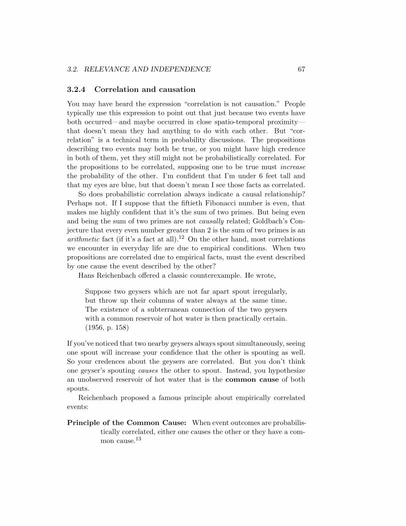
Hans Reichenbach offered a classic counterexample. He wrote,

Suppose two geysers which are not far apart spout irregularly,but throw up their columns of water always at the same time.The existence of a subterranean connection of the two geyserswith a common reservoir of hot water is then practically certain.(1956, p. 158)

If you’ve noticed that two nearby geysers always spout simultaneously, seeingone spout will increase your confidence that the other is spouting as well.So your credences about the geysers are correlated. But you don’t thinkone geyser’s spouting causes the other to spout. Instead, you hypothesizean unobserved reservoir of hot water that is the common cause of bothspouts.

Reichenbach proposed a famous principle about empirically correlatedevents:

Principle of the Common Cause: When event outcomes are probabilis-tically correlated, either one causes the other or they have a com-mon cause.13


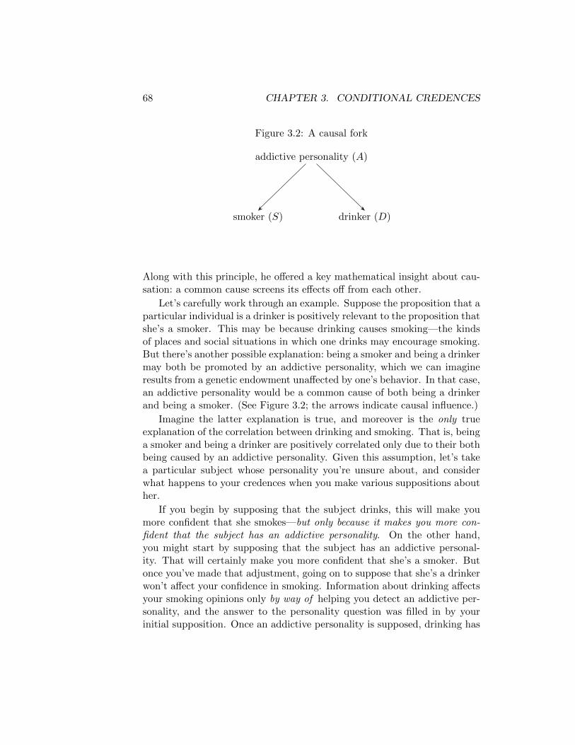
Figure 3.2: A causal fork

smoker (S) drinker (D)

addictive personality (A)

Along with this principle, he offered a key mathematical insight about cau-sation: a common cause screens its effects off from each other.

Let’s carefully work through an example. Suppose the proposition that aparticular individual is a drinker is positively relevant to the proposition thatshe’s a smoker. This may be because drinking causes smoking—the kindsof places and social situations in which one drinks may encourage smoking.But there’s another possible explanation: being a smoker and being a drinkermay both be promoted by an addictive personality, which we can imagineresults from a genetic endowment unaffected by one’s behavior. In that case,an addictive personality would be a common cause of both being a drinkerand being a smoker. (See Figure 3.2; the arrows indicate causal influence.)

Imagine the latter explanation is true, and moreover is the only trueexplanation of the correlation between drinking and smoking. That is, beinga smoker and being a drinker are positively correlated only due to their bothbeing caused by an addictive personality. Given this assumption, let’s takea particular subject whose personality you’re unsure about, and considerwhat happens to your credences when you make various suppositions abouther.

If you begin by supposing that the subject drinks, this will make youmore confident that she smokes—but only because it makes you more con-fident that the subject has an addictive personality. On the other hand,you might start by supposing that the subject has an addictive personal-ity. That will certainly make you more confident that she’s a smoker. Butonce you’ve made that adjustment, going on to suppose that she’s a drinkerwon’t affect your confidence in smoking. Information about drinking affectsyour smoking opinions only by way of helping you detect an addictive per-sonality, and the answer to the personality question was filled in by yourinitial supposition. Once an addictive personality is supposed, drinking has


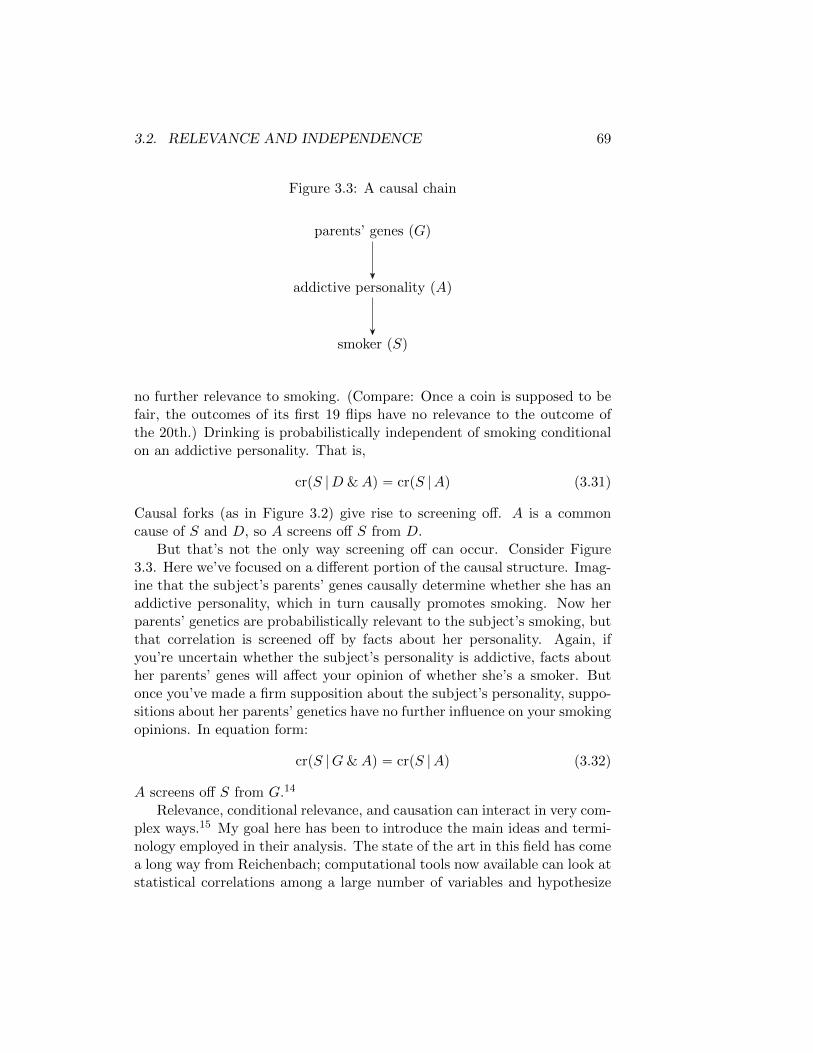
Figure 3.3: A causal chain

addictive personality (A)

smoker (S)

parents’ genes (G)

no further relevance to smoking. (Compare: Once a coin is supposed to befair, the outcomes of its first 19 flips have no relevance to the outcome ofthe 20th.) Drinking is probabilistically independent of smoking conditionalon an addictive personality. That is,

crpS |D & Aq “ crpS |Aq (3.31)

Causal forks (as in Figure 3.2) give rise to screening off. A is a commoncause of S and D, so A screens off S from D.

But that’s not the only way screening off can occur. Consider Figure3.3. Here we’ve focused on a different portion of the causal structure. Imag-ine that the subject’s parents’ genes causally determine whether she has anaddictive personality, which in turn causally promotes smoking. Now herparents’ genetics are probabilistically relevant to the subject’s smoking, butthat correlation is screened off by facts about her personality. Again, ifyou’re uncertain whether the subject’s personality is addictive, facts abouther parents’ genes will affect your opinion of whether she’s a smoker. Butonce you’ve made a firm supposition about the subject’s personality, suppo-sitions about her parents’ genetics have no further influence on your smokingopinions. In equation form:

crpS |G & Aq “ crpS |Aq (3.32)

A screens off S from G.14

Relevance, conditional relevance, and causation can interact in very com-plex ways.15 My goal here has been to introduce the main ideas and termi-nology employed in their analysis. The state of the art in this field has comea long way from Reichenbach; computational tools now available can look atstatistical correlations among a large number of variables and hypothesize


a causal structure lying beneath them. The resulting causal diagrams areknown as Bayes Nets, and have practical applications from satellites tohealth care to car insurance to college admissions.

And as for Reichenbach’s Principle of the Common Cause? It remainshighly controversial.

3.3 Conditional credences and conditionals

I want to circle back and get clearer on the nature of conditional credence.First, it’s important to note that the conditional credences we’ve been dis-cussing are indicative, not subjunctive. The distinction is familiar from thetheory of conditional propositions. Compare:

If Shakespeare didn’t write Hamlet, someone else did.If Shakespeare hadn’t written Hamlet, someone else would have.

The former conditional is indicative, while the latter is subjunctive. Typi-cally one evaluates the truth of a conditional by considering possible worldsin which the antecedent is satisfied, then seeing if those worlds make the con-sequent true as well. When you evaluate an indicative conditional, you’rerestricted to considering worlds among your doxastic possibilities. Evalu-ating a subjunctive conditional, on the other hand, permits you to engagein counterfactual reasoning involving worlds you’ve actually ruled out. Sofor the subjunctive conditional above, you can consider worlds that makethe antecedent true because Hamlet never exists. But for the indicativeconditional, you have to take into account that Hamlet does exist, andentertain only worlds in which that’s true. So you consider bizarre “author-conspiracy” worlds which, while far-fetched, satisfy the antecedent and areamong your current doxastic possibilities. In the end, I’m guessing you takethe indicative conditional to be true but the subjunctive to be false.

Now suppose I ask for your credence in the proposition that someonewrote Hamlet, conditional on the supposition that Shakespeare didn’t. Thisvalue will be high, again because Hamlet exists. In assigning this condi-tional credence, you aren’t bringing into consideration possible worlds you’dotherwise ruled out (such as Hamlet-free worlds). Instead, you’re focusingin on the narrow set of author-conspiracy worlds you currently entertain. Aswe saw in Figure 3.1, assigning a conditional credence strictly narrows theworlds under consideration; it’s doesn’t expand your attention to worlds pre-viously ruled out. Thus the conditional credences discussed in this book—and typically discussed in the Bayesian literature—are indicative rather thansubjunctive.16

3.3. CONDITIONAL CREDENCES AND CONDITIONALS 71

Are there more features of conditional propositions that can help us un-derstand conditional credences? Might we understand conditional credencesin terms of conditionals? Initiating his study of conditional degrees of belief,F.P. Ramsey warned against assimilating them to conditional propositions:

We are also able to define a very useful new idea—“the degree ofbelief in p given q”. This does not mean the degree of belief in“If p then q”, or that in “p entails q”, or that which the subjectwould have in p if he knew q, or that which he ought to have.(1931, p. 82)

Yet many authors failed to heed Ramsey’s warning. It’s very temptingto equate conditional credences with some simple combination of conditionalpropositions and unconditional credences. For example, when I ask, “Howconfident are you in P given Q?”, it’s easy to hear that as “Given Q, howconfident are you in P?” or just “If Q is true, how confident are you in P?”This simple slide might suggest that

crpP |Qq “ r is equivalent to QÑ crpP q “ r (3.33)

Here I’m using the symbol “Ñ” to represent some kind of conditional. Forthe reasons discussed above, it should be an indicative conditional. Butit need not be the material conditional symbolized by “Ą”; many authorsthink the material conditional’s truth-function fails to accurately representthe meaning of natural-language indicative conditionals.

There are two problems with the proposal of Equation (3.33). First,it gets the logic of conditional credences wrong. On most theories of theindicative conditional (and certainly if Ñ is the material conditional),

X Ñ Z and Y Ñ Z jointly entail pX _ Y q Ñ Z (3.34)

for any propositions X, Y , and Z. Thus for any propositions A, B, and Cand constant k we have

AÑ rcrpCq “ ks and B Ñ rcrpCq “ ks entail pA_Bq Ñ rcrpCq “ ks(3.35)

Combining Equations (3.33) and (3.35) yields

crpC |Aq “ k and crpC |Bq “ k entail crpC |A_Bq “ k (3.36)

which is false. Not only can one design a credence distribution satisfy-ing the probability axioms and Ratio Formula such that crpC |Aq “ k and


crpC |Bq “ k but crpC |A_Bq ‰ k; one can even describe real-life examplesin which it’s rational for an agent to assign such a distribution. (See Exercise3.12.) The failure of Equation (3.36) is another case in which credences con-found expectations developed by our experiences with classificatory terms.

The second problem with the equivalence proposed by Equation (3.33)is that it’s just bizarre. crpP |Qq “ r says that when the agent supposesproposition Q is true, her confidence in P is r. Q Ñ crpP q “ r says thatif Q is actually true, the agent’s unconditional credence in P is actuallyr. These claims are oddly mismatched, as brought out by the followingexample: Right now you’re highly confident that you’ll live for the nextyear (proposition P ). Conditional on the supposition that the sun explodedten seconds ago (proposition Q), you are considerably less confident aboutyour life expectancy. But this doesn’t mean that if (unbeknownst to you)the sun did explode ten seconds ago, you are right now unconfident thatyou’ll be alive in a year.

Perhaps we’ve mangled the transition from conditional credences to con-ditional propositions. Perhaps we should hear “How confident are you inP given Q?” as “How confident are you in ‘P , given Q’?” which is in turn“How confident are you in ‘If Q, then P ’?” Maybe a conditional credenceis a credence in a conditional. Or perhaps more weakly: an agent assigns aparticular conditional credence value whenever she unconditionally assignsthat value to a conditional. In symbols, the proposal is

crpP |Qq “ r is equivalent to crpQÑ P q “ r (3.37)

for any propositions P and Q, any credence distribution cr, and some indica-tive conditional Ñ. Reading Equation (3.37) left-to-right offers a possibleanalysis of conditional credences. On the other hand, some philosophers oflanguage have read the right-to-left direction as a key to analyzing indicativeconditionals.17

We can quickly show that Equation (3.37) fails if “Ñ” is read as thematerial conditional Ą. Under the material reading, the proposal entailsthat

crpP |Qq “ crpQ Ą P q (3.38)

Using the probability calculus and Ratio Formula, we can show that Equa-tion (3.38) holds only when crpP q “ 1 (and Q is nonzero). This is a trivialityresult : it shows that Equation (3.38) can hold only for the narrow range ofpropositions P of which the agent is absolutely certain. Equation (3.38) doesnot express a truth that holds for all conditional credences in all proposi-tions; nor does Equation (3.37) when “Ñ” is read materially.

3.3. CONDITIONAL CREDENCES AND CONDITIONALS 73

Equation (3.37) can be saved from this objection by construing its “Ñ”as something other than a material conditional. But Lewis (1976) provideda clever objection that works whichever conditional Ñ we choose. Begin byselecting arbitrary propositions P and Q. We then derive the following fromthe proposal on the table:

crpQÑ P q “ crpP |Qq rfrom Equation (3.37)s (3.39)

crpQÑ P |P q “ crpP |Q & P q rsee belows (3.40)

crpQÑ P |P q “ 1 rQ & P entails P s (3.41)

crpQÑ P | „P q “ crpP |Q &„P q rsee belows (3.42)

crpQÑ P | „P q “ 0 rQ &„P refutes P s (3.43)

crpQÑ P q “ crpQÑ P |P q ¨ crpP q `

crpQÑ P | „P q ¨ crp„P q rLaw of Tot. Prob.s (3.44)

crpQÑ P q “ 1 ¨ crpP q ` 0 ¨ crp„P q [(3.41), (3.43), (3.44)] (3.45)

crpQÑ P q “ crpP q (3.46)

crpP |Qq “ crpP q [(3.39)] (3.47)

Some of these lines require explanation. The idea of lines (3.40) and (3.42)is this: We’ve already seen that a credence distribution conditional on aparticular proposition satisfies the probability axioms. This suggests thatwe should think of a distribution conditional on a proposition as being justlike any other credence distribution. (We’ll see more reason to think this inChapter 4, note 3.) So a distribution conditional on a proposition shouldsatisfy the proposal of Equation (3.37) as well. If you conditionally supposeX, then under that supposition you should assign Y Ñ Z the same credenceyou would assign Z were you to further suppose Y . In other words,

crpY Ñ Z |Xq “ crpZ |Y & Xq (3.48)

In line (3.40) the roles of X, Y , and Z are played by P , Q, and P ; in line(3.42) it’s „P , Q, and P .

Lewis has offered us another triviality result. Assuming the probabilityaxioms and Ratio Formula, the proposal in Equation (3.37) can hold onlyfor propositions P and Q such that crpP |Qq “ crpP q. In other words,it can hold only for propositions the agent takes to be independent. Or(taking things from the other end), the proposed equivalence can hold forall the conditionals an agent entertains only if the agent takes every pair ofpropositions in L to be independent!

So a rational agent’s conditional credence will not in general equal herunconditional credence in a conditional. This is not to say that conditional


credences have nothing to do with conditionals. A popular idea now usuallycalled “Adams’ Thesis” (Adams 1965) holds that an indicative conditionalQÑ P is acceptable to a degree equal to crpP |Qq.18 But we cannot main-tain that an agent’s conditional credence is equal to her credence that someconditional is true.

This brings us back to a proposal I discussed in Chapter 1. One mighttry to relate degrees of belief to binary beliefs by suggesting that wheneveran agent has an r-valued credence, she has a (binary) belief with r as part ofits content. Working out this proposal for conditional credences reveals howhopeless it is. Suppose an agent assigns crpP |Qq “ r. Would we suggestthat the agent believes that if Q, then the probability of P is r? This getsthe logic of conditional credences wrong. Perhaps the agent believes thatthe probability of “if P , then Q” is r? Lewis’s argument dooms this idea.

I said in Chapter 1 that the numerical value of an unconditional degree ofbelief is an attribute of the attitude taken towards the proposition, not a con-stituent of that proposition itself. As for conditional credences, crpP |Qq “ rdoes not say that an agent takes some attitude towards a conditional witha probability value in its consequent. Nor does it say that the agent takessome attitude towards a single, conditional proposition composed of P andQ. crpP |Qq “ r says that the agent takes an r-valued attitude towards anordered pair of propositions—neither of which need refer to the number r.

3.4 Exercises

Unless otherwise noted, you should assume when completing these exercisesthat the cr-distributions under discussion satisfy the probability axioms andRatio Formula. You may also assume that whenever a conditional cr ex-pression occurs, the condition has a nonzero unconditional credence so thatthe conditional credence is well-defined.

Problem 3.1. Suppose there are 30 people in a room. For each person,you’re equally confident that their birthday falls on any of the 365 days in ayear. (You’re certain none of them was born in a leapyear.) Your credencesabout each person’s birthday are independent of your credences about allthe other people’s birthdays. How confident are you that at least two peoplein the room share a birthday? (Hint: First calculate your credence that notwo people in the room share a birthday.)

Problem 3.2. One might think that real humans only assign credences thatare rational numbers—and perhaps only rational numbers involving rela-tively small whole-number numerators and denominators. But we can write

3.4. EXERCISES 75

down simple conditions that require an irrational-valued credence function.For example, take these three conditions:

1. crpY |Xq “ crpX _ Y q

2. crpX & Y q “ 1{4

3. crp„X & Y q “ 1{4

Show that there is exactly one credence distribution over language L withatomic propositions X and Y that satisfies all three of these conditions, andthat that distribution contains irrational-valued credences.˚

Problem 3.3. Prove that credences conditional on a particular propositionform a probability distribution. That is, prove that for any proposition Rin L such that crpRq ą 0, the following three conditions hold:

(a) For any proposition P in L, crpP |Rq ě 0.

(b) For any tautology T in L, crpT |Rq “ 1.

(c) For any mutually exclusive propositions P and Q in L,crpP _Q |Rq “ crpP |Rq ` crpQ |Rq.

Problem 3.4. Pink gumballs always make my sister sick. (They remind herof Pepto Bismol.) Blue gumballs make her sick half of the time (they justlook unnatural), while white gumballs make her sick only one-tenth of thetime. Yesterday, my sister bought a single gumball from a machine that’sone-third pink gumballs, one-third blue, and one-third white. The gumballmade her sick. Applying the version of Bayes’ Theorem in Equation (3.12),how confident should I be that my sister got a pink gumball yesterday?

Problem 3.5. (a) Prove Bayes’ Theorem from the probability axioms andRatio Formula. (Hint: Start by using the Ratio Formula to write downexpressions involving crpH & Eq and crpE & Hq.)

(b) Exactly which unconditional credences must we assume to be positivein order for your proof to go through?

(c) Where exactly does your proof rely on the probability axioms (and notjust the Ratio Formula)?

˚I owe this problem to Branden Fitelson.


Problem 3.6. Once more, consider the probabilistic credence distributionspecified by this stochastic truth-table (from Exercise 2.5):

P Q R cr

T T T 0.1

T T F 0.2

T F T 0

T F F 0.3

F T T 0.1

F T F 0.2

F F T 0

F F F 0.1

Answer the following questions about this distribution:

(a) What is crpP |Qq?

(b) Is Q positively relevant to P , negatively relevant to P , or probabilisti-cally independent of P?

(c) What is crpP |Rq?

(d) What is crpP |Q & Rq?

(e) Conditional on R, is Q positively relevant to P , negatively relevant toP , or probabilistically independent of P?

(f) Does R screen off P from Q? Explain why or why not.

Problem 3.7. Prove that all the alternative statements of probabilisticindependence in Equations (3.15) through (3.18) follow from our originalindependence definition. That is, prove that each Equation (3.15) through(3.18) follows from Equation (3.14). (Hint: Once you prove that a particularequation follows from Equation (3.14), you may use it in subsequent proofs.)

Problem 3.8. Show that probabilistic independence is not transitive. Thatis, provide a single probability distribution on which all of the following aretrue: X is independent of Y , and Y is independent of Z, but X is not inde-pendent of Z. Show that your distribution satisfies all three conditions. (Foran added challenge, have your distribution assign every state-description anonzero unconditional credence.)

3.4. EXERCISES 77

Problem 3.9. In the text we discussed what makes a pair of propositionsprobabilistically independent. If we have a larger collection of propositions,what does it take to make them all independent of each other? You mightthink all that’s necessary is pairwise independence—for each pair within theset of propositions to be independent. But pairwise independence doesn’tguarantee that each proposition will be independent of combinations of theothers.

To demonstrate this fact, describe a real-world example (spelling out thepropositions represented by X, Y , and Z) in which it would be rational foran agent to assign credences meeting all four of the following conditions:

1. crpX |Y q “ crpXq

2. crpX |Zq “ crpXq

3. crpY |Zq “ crpY q

4. crpX |Y & Zq ‰ crpXq

Show that your example satisfies all four conditions.

Problem 3.10. Using the program PrSAT referenced in the Further Read-ings for Chapter 2, find a probability distribution satisfying all the condi-tions in Exercise 3.9, plus the following additional condition: Every state-description expressible in terms of X, Y , and Z must have a non-zero un-conditional probability.

Problem 3.11. After laying down probabilistic conditions for a causal fork,Reichenbach demonstrated that a causal fork induces correlation. Considerthe following four conditions:

1. crpA |Cq ą crpA | „Cq

2. crpB |Cq ą crpB | „Cq

3. crpA & B |Cq “ crpA |Cq ¨ crpB |Cq

4. crpA & B | „Cq “ crpA | „Cq ¨ crpB | „Cq

(a) Assuming C is the common cause of A and B, explain what each of thefour conditions means in terms of relevance, independence, conditionalrelevance, or conditional independence.

(b) Prove that if all four conditions hold, then crpA & Bq ą crpAq ¨ crpBq.(This is a tough one!)


Problem 3.12. In Section 3.3 I pointed out that the following statement(labeled Equation (3.36) there) is false:

crpC |Aq “ k and crpC |Bq “ k entail crpC |A_Bq “ k

(a) Describe a real-world example (involving dice, or cards, or somethingmore interesting) in which it’s rational for an agent to assign crpC |Aq “k and crpC |Bq “ k but crpC |A _ Bq ‰ k. Show that your examplemeets this description.

(b) Prove that if A and B are mutually exclusive, then whenever crpC |Aq “k and crpC |Bq “ k it’s also the case that crpC |A_Bq “ k.

Problem 3.13. Fact: For any propositions P and Q, if crpQq ą 0 thencrpQ Ą P q ě crpP |Qq.

(a) Use a stochastic truth-table built on propositions P and Q to prove thisfact.

(b) Show that Equation (3.38) in Section 3.3 entails that crpP q “ 1.

3.5 Further reading

Introductions and Overviews

Todd A. Stephenson (2000). An Introduction to Bayesian Net-work Theory and Usage. Tech. rep. 03. IDIAP

Section 1 provides a nice, concise overview of what a Bayes Net is and how itinteracts with conditional probabilities. (Note that the author uses A,B toexpress the conjunction of A and B.) Things get fairly technical after thatas he covers algorithms for creating and using Bayes Nets. Sections 6 and7, though, contain real-life examples of Bayes Nets for speech recognition,Microsoft Windows troubleshooting, and medical diagnosis.

Classic Texts

Hans Reichenbach (1956). The Principle of Common Cause.In: The Direction of Time. University of California Press,pp. 157–160

Article in which Reichenbach introduces his account of common causesin terms of screening off. (Note that Reichenbach uses a period to ex-press conjunction, and a comma rather than a vertical bar for conditionalprobabilities—what we would write as crpA |Bq he writes as PpB,Aq.)

NOTES 79

David Lewis (1976). Probabilities of Conditionals and Condi-tional Probabilities. The Philosophical Review 85, pp. 297–315

Article in which Lewis presents his triviality argument concerning probabil-ities of conditionals.

Extended Discussion

Frank Arntzenius (1993). The Common Cause Principle. PSA1992 2, pp. 227–237

Presents a number of objections to Reichenbach’s Principle of the CommonCause, with citations (when the objections aren’t original to Arntzeniushimself).

Alan Hajek and Ned Hall (1994). The Hypothesis of the Con-ditional Construal of Conditional Probability. In: Probabil-ity and Conditionals: Belief Revision and Rational Decision.Ed. by Ellery Eells and Brian Skyrms. Cambridge Studiesin Probability, Induction, and Decision Theory. CambridgeUniversity Press, pp. 75–112

Hajek and Hall extensively assess views about conditional credences andcredences in conditionals in light of Lewis’s and other triviality results.

Notes

1Here’s a good way to double-check that 6 & E is equivalent to 6: Remember thatequivalence is mutual entailment. Clearly 6 & E entails 6. Going in the other direction, 6entails 6, but 6 also entails E. So 6 entails 6 &E. When evaluating conditional credencesusing the Ratio Formula we’ll often find ourselves simplifying a conjunction down to justone or two of its conjuncts. To make this work, the conjunct that remains has to entaileach of the conjuncts that was removed.

2Some authors take advantage of this fact to formalize probability theory in exactlythe opposite order from what I’ve pursued here. They begin by introducing conditionalprobabilites or credences and subject them to a number of constraints somewhat like Kol-mogorov’s axioms. All the desired rules for unconditional credences are then obtainedby introducing the single constraint that crpP q “ crpP |Tq. Just as the Ratio Formulahelps us transform constraints on unconditional credences into constraints on conditionalcredences, this rule transforms constraints on conditionals into constraints on uncondi-tionals. For examples of this conditional-probability-first approach, see (Popper 1955),(Renyi 1970), and (Roeper and Leblanc 1999).

80 NOTES

3Bayes never published the theorem; Richard Price found it in Bayes’ notes and pub-lished it after Bayes’ death in 1761. Pierre-Simon Laplace independently rediscovered thetheorem later on and was responsible for much of its early popularization.

4In everyday English “likely” is a synonym for “probable”. Yet R.A. Fisher intro-duced the technical term “likelihood” to represent a particular kind of probability—theprobability of some evidence given a hypothesis. This somewhat peculiar terminology hasstuck.

5Quoted in (Galavotti 2005, p. 51).6I’m assuming throughout this discussion that P , „P , Q, and „Q all have non-zero

unconditional credences so that the relevant conditional credences are well-defined.7Different authors define “screening off” in different ways. For example, while condi-

tional independence is interesting only when the propositions in question are uncondition-ally correlated, most authors leave out the requirement that P be unconditionally relevantto Q. (I suppose one could alter my definition so that unconditionally-independent P andQ would count as trivially screened off by anything.)

Many authors will say that R screens off P and Q only when P and Q are independentnot only conditionally on R but also conditionally on „R. This is part of a more generalview on which propositions are simply dichotomous random variables (see Chapter 2,note 6) and a random variable X screens off Y from Z only if Y and Z are independentconditional on every possible value of X. If one takes this kind of position, then in Bob’scredence function I does not count as screening H off from C, because H and C arecorrelated conditional on „I. Adopting this alternate definition would lead us to re-characterize some of the examples I’ll soon discuss, but would not make any difference tothe causal examples we’ll eventually consider.

8Not to be confused with the Rambler’s Fallacy: I’ve said so many false things in arow, the next one must be true!

920 flips of a fair coin provide a good example of what statisticians call IID trials.“IID” stands for “independent, identically distributed.” Each of the coin flips is proba-bilistically independent of all the others; information about the outcomes of other coinflips doesn’t change the probability that a particular flip will come up heads. The flipsare identically distributed because each has the same probability of producing a headsoutcome.

Anyone who goes in for the Gambler’s Fallacy and thinks that future flips will makeup for past outcomes is committed to the existence of some mechanism by which futureflips can respond to what happened in the past. Understanding that no such mechanismexists leads one to treat repeated flips of the same coin as IID.

10I learned about the Jeter/Justice example from the Wikipedia page on Simpson’sParadox. (The batting data for the two hitters is widely available.) The UC Berkeleyexample was brought to the attention of philosophers by (Cartwright 1979).

11An analogy: Suppose we each have some gold bars and some silver bars. Each goldbar you’re holding is heavier (and therefore more valuable) than each of my gold bars.Each silver bar you’re holding is heavier (and more valuable) than each of my silver bars.Then how could I possibly be richer than you? If I have many more gold bars than you,while you have more silver than I.

12You may be concerned that arithmetic facts are true in every possible world, andso cannot rationally receive nonextreme credences, and so cannot be probabilisticallycorrelated. We’ll come back to that concern in Chapter XXX.

13I’m playing a bit fast and loose with the objects of discussion here. Throughout thischapter we’re considering correlations in an agent’s credence distribution. Reichenbach

NOTES 81

was concerned not with probabilistic correlations in an agent’s credences but instead withcorrelations in objective frequency or chance distributions (more about which in Chapter5). But presumably if the Principle of the Common Cause holds for objective probabilitydistributions, that provides an agent who views particular propositions as empiricallycorrelated some reason to suppose that the events described in those propositions eitherstand as cause to effect or share a common cause.

14You might worry that Figure 3.3 presents a counterexample to Reichenbach’s Principleof the Common Cause, because G and S are unconditionally correlated yet G doesn’t causeS and they have no common cause. It’s important to the principle that the causal relationsneed not be direct ; for Reichenbach’s purposes G counts as a cause of S even though it’snot the immediate cause of S.

15Just to indicate a few more complexities that can arise: One can have a common cause(an “indirect” common cause) that doesn’t screen off its effects from each other. For ex-ample, if we imagine merging Figures 3.2 and 3.3 to show how the subject’s parents’ genesare a common cause of both smoking and drinking by way of her addictive personality, itis possible to arrange the numbers so that her parents’ genetics don’t screen off smokerfrom drinker. Even more complications arise if some causal arrows do end-arounds pastothers—what if in addition to the causal structure just described, the parents’ geneticstend to make them smokers which in turn influences the subject’s smoking behavior?

16One could study a kind of attitude different from the conditional credences in thisbook, and to which the Ratio Formula applies—something like a subjunctive degree ofbelief. Joyce (1999) does exactly that, but is careful to distinguish his analysandum fromstandard conditional degrees of belief.

17While Equation (3.37) has often been read as an analysis in one direction or another,it could also be read as a normative constraint: If an agent is rational, she will assign thesame value to crpP |Qq as she does to crpQÑ P q for any P and Q. Since our argumentsagainst Equation (3.37) will be based on the probability axioms and Ratio Formula, andsince we assume that rational credences also satisfy those constraints, such a normativeinterpretation would ultimately be vulnerable to our arguments as well.

18Interestingly, this idea is often traced back to a suggestion in Ramsey, known as“Ramsey’s test”. (Ramsey 1929/1990, p. 155n)

Documents

Conditional Credences - Fitelson