RISK SENSITIVITY Lara Buchak, Princeton University

Abstract: In this paper, I explore the question of whether decision theory overly constrains the attitudes that agents can take towards risk. In the first section, I show that agents with a certain sensitivity to risk cannot be represented by classical decision theory. The standard notion of risk aversion (i.e. diminishing marginal utility) fails to account for the preferences of these “risk sensitive” agents, and although the method of the Representation Theorem appears to yield a representation of their preferences, it gives the wrong answers in certain cases. I then show that these agents fail to satisfy a certain axiom of decision theory – the “sure thing principle” – and thus their preferences are incoherent on the standard framework. In the second section, I consider arguments purporting to show that risk sensitive agents should count as irrational. In particular, I present Dutch-book-style arguments against risk sensitivity. However, these arguments fail for two important reasons: they assume symmetry between gain and loss, and they assume that the Dutch bookie has information that the agent does not have. I conclude that although risk sensitive agents have incoherent preferences, they are not thereby irrational. Therefore, agents can have certain sets of intuitively plausible, rational preferences and yet not be representable on the standard decision-theoretic framework.

Introduction

The Representation Theorem is a useful tool in decision theory: it provides a way

by which we can take an agent’s preferences over certain prospects, and arrive at a utility

function that accurately reflects those preferences; a function such that a prospect will

have a higher expected utility value than another prospect if and only if the agent prefers

the former prospect to the latter. Ingeniously, it takes us from ordinal preferences to

cardinal utilities.i In order to do this, it relies on several basic axioms. Sets of

preferences that do not obey all the axioms are incoherent on the theorem, and agents

holding these preferences cannot be represented using the theorem.

Certainly no decision theorist would claim that decision theory is descriptively

adequate; there are many examples of experimental situations in which people make

choices that reveal preferences that violate these basic axioms. However, decision theory

is supposed to describe ideally rational agents: agents whose preferences satisfy certain

axioms that are constitutive of rationality. Lest this sound like an empty theory, it is

i Richard Jeffrey uses the term “desirability” in place of “utility.” I will use the two terms interchangeably.

2

worth pointing out that the axioms are supposed to be intuitively plausible, and are

supposed to be such that thoughtful agents would subscribe to them if they were

presented with decisions in a clear enough light, when the agents are in a discerning

frame of mind and in possession of perfect mathematical knowledge, and so forth. In

other words, the agents that decision theory describes are supposed to have some claim to

being rational that other agents do not; it is incumbent on rational agents – insofar as they

can claim to be rational – to adjust their preferences to satisfy the axioms of decision

theory.

In this paper, I will explore the question of whether people with certain

(intuitively plausible) attitudes towards risk can be represented by classical decision

theory. In the first section, I will show that they cannot be so represented; the standard

notion of diminishing marginal utility fails to account for the preferences of these agents,

and although the method of the Representation Theorem appears to yield a representation

of their preferences, it gives the wrong answers in certain cases. I will then show that

these agents fail to satisfy a certain axiom of decision theory. Thus, their preferences are

incoherent. In the second section, I will explore arguments that claim to show that

rational agents should satisfy this axiom; that is, that risk sensitive people are irrational.

However, I claim that these arguments fail. Thus, although risk sensitive agents have

incoherent preferences, they are not thereby irrational.

Can risk sensitive people be represented?

Different agents take different attitudes towards risk, and on the face of it, there is

nothing irrational about preferring to avoid risk. It is a generally uncontroversial

phenomenon that for many people, gambles are worth less than their expected monetary

value; that is, that if a gamble between $x and $y is expected to yield $z on average, then

an agent may prefer simply receiving $z to taking that gamble. For example, an agent

may be willing to pay only $25 for a gamble that yields $0 if a fair coin lands heads and

$100 if the coin lands tails, even though the gamble will yield $50 on average.

This phenomenon could admit of two very different psychological explanations.

The standard explanation is that of diminishing marginal utility. This explanation holds

that, as some people think about the prospect of having more money, additional amounts

3

of money add less value. For example, if I am going to get $50, then getting an extra $50

doesn’t increase the value of the prospect as much as it does when I am initially not going

to get anything. Put another way, I assign value not to increments of money, but to final

dollar amounts, and as the dollar amounts increase, each increment adds less value.

I will call the second explanation the risk sensitivity explanation. This

explanation holds that one possible reason that the utility of a gamble expected to yield

$50 on average is less than the utility of $50 is that when an agent evaluates the

attractiveness of a gamble, he attaches value not just to the final dollar amounts he might

receive, but to the probability he has of receiving each amount. In general, a sure thing is

worth more to him than a gamble that will yield the same utility on average; roughly

speaking, the fact that he might get the higher outcome does not entirely make up for the

fact that he might get the lower outcome. On the risk sensitivity explanation, an agent

could still have a diminishing marginal utility function, or not value money in a linear

way; what the risk sensitivity explanation entails is that diminishing marginal utility does

not provide the whole explanation.

Of course, decision theory is not necessarily interested in psychological facts

about the agents it describes; in particular, neither the Representation Theorem nor its

axioms need rely on these types of facts. It merely shows that, given an agent’s

preferences over prospects, we can arrive at a utility function that accords with – or

correctly predicts – the way an agent (or an idealized version of that agent) makes

decisions. So if the two different psychological explanations map onto the same data,

then for our purposes, they are the same, and it does not matter which one accords better

with human psychology. If they map onto the same data, then even if some people

experience themselves as risk sensitive – and find the diminishing marginal utility

explanation counterintuitive – these people can still be represented as standard decision

theoretic agents. In other words, if we can use diminishing marginal utility functions to

capture the way so-called risk sensitive people make decisions, then that is all we need;

risk sensitive people will obey the axioms of standard decision theory, and consequently

will have preferences that are accurately and adequately represented by the

Representation Theorem. We will be able to take their preferences over gambles and

arrive at a utility function that will accord with their preferences. So our first task is

4

determining whether the preferences of risk-sensitive people can be captured using

diminishing marginal utility functions.

To see whether our intuitive notion of risk sensitivity can be fully captured by the

notion of diminishing marginal utility, let me first explain formally how a risk sensitive

agent might value gambles. On Ramsey’s and Jeffrey’s decision theory, the desirability

of a gamble between two options is a weighted average of the desirability of those

options. Thus, the desirability of the gamble between A and B is p(des(A)) + (1 –

p)(des(B)) or, equivalently, des(B) + p[des(A) – des(B)]. Taking B to be the less (or

equally) desirable option, this second formulation merely says that the desirability of the

gamble will be the minimum desirability guaranteed plus the amount by which the agent

could do better, weighted by the probability of doing that much better. I will call an

agent risk sensitive if the chance of getting the better option will not be weighted quite as

highly; that is, if the weight she gives to how much she might improve her chances will

be a function of the probability of improving her chances. One way to formulate this

mathematically, put forth by Kahneman and Tversky, is to say that the desirability of {pA

⊕ (1 – p)B}ii will be des(B) + f(p)(des(A) – des(B)), where f is an agent’s “probability

function” adhering to the parameters f(0) = 0, f(1) = 1, f is non-decreasing, and 0 ≤ f(p) ≤

1 for all p.iii The standard (risk insensitive) agent will just be a special case of this

formula with f(p) = p, and for a risk sensitive agent, we will always have f(p) ≤ p (with

f(p) < p for some p). Put loosely, the uncertainty itself decreases the desirability of a

gamble for a risk sensitive agent. In effect, the interval by which the agent might

improve her lot shrinks not merely by her chance of getting the better prize, but by a

function of this chance, which reflects her attitude towards probabilities.

We can see why this formulation is intuitively plausible. As an agent approaches

a gamble, she is likely to think about the three factors which define the gambleiv: the

ii To avoid confusion, I will use the ⊕ symbol between the component parts of a gamble and the + symbol between expressions that stand for numbers. iii Kahneman, Daniel and Tversky, Amos. Prospect Theory: An Analysis of Decision under Risk. Econometrica, Vol. 42, No. 2 (March 1979). Pg. 276. Although I use the same equation as Kahneman and Tversky, I do not focus on the empirical work related to the equation; I only need the assumption that this is a plausible way for agents to calculate the desirability of gambles, which the empirical work supports. Thus, the reader should not take what I say to have too much direct connection with the work of Kahneman and Tversky. iv For the moment, I am only speaking of gambles between two options.

5

worst she can do, how much she stands to gain over the minimum amount, and her

chances of improving over the minimum. It is plausible that different agents have

different attitudes towards each of these factors, not just towards the first two. For

example, it is plausible that two agents who both attach a certain value to $100 and a

certain value to $0 will not both attach the same value to a coin flip between $0 and $100;

one may think the fact that he only has a 50% chance of winning the better prize

diminishes the worth of the gamble more than the other does.

Let me clear up a possible misunderstanding by answering an immediate

objection. The objection points out that, even for agents who are sensitive to risk, the

fact that outcomes are offered as the result of gambles need not always affect the

desirabilities of those outcomes, particularly if the outcomes are more fine-grained than

the agent’s preferences. Consider the gamble that yields a 2003 dollar bill if a fair coin

lands heads and a 2004 dollar bill if a fair coin lands tails. Assuming there is nothing

special about either bill, it would seem irrational to value this gamble less than receiving

either dollar bill (or a nondescript dollar bill) for certain. And it seems that my risk-

sensitive agents must be committed to discounting both possible outcomes simply

because the outcomes are not guaranteed.

This objection is wrong-headed, however. In this case, since both the 2003 dollar

bill and the 2004 dollar bill have the same desirability as $1, the gamble {½(2003 dollar)

⊕ ½(2004 dollar)} will have a desirability of des(2003 dollar) + f(½)[des(2004 dollar) –

des(2003 dollar)]. This is equivalent to des($1) + f(½)(des($1) – des($1)) = des($1) + 0 =

des($1). Thus, the gamble will have the same desirability as the sure-thing dollar. This

holds because it is not the values of the outcomes themselves that a risk-sensitive agent

discounts, but rather the intervals between the values. In this case, there is no difference

in value between the two possible outcomes, so the interval that gets discounted has

length zero. Any gamble whose outcomes all have the same value must necessarily have

that value itself. Furthermore, because of the constraint that 0 ≤ f(p) ≤ 1, the desirability

of a gamble will never be less than the desirability of all of its constituent outcomes, and

it will never be greater than the desirability of all of its constituent outcomes; the best and

worst possible outcomes are upper and lower bounds on the desirability of a gamble.

6

To further flesh out the proposal, let’s consider another example of how a risk

sensitive agent could value some gambles. Assume that her f-function is f(p) = p2, and

that she values money linearly (for the sake of simplicity, we will assume that $x has a

value of x). Then a coin flip between $0 and $4 will be worth des($0) + (½)2[des($4) –

des($0)] = 0 + ¼(4 – 0) = 1. That is, it will have the same desirability as $1. Similarly, a

coin flip between $0 and $1 will be worth 25 cents. A coin flip between $1 and $4 will

be worth $1.75. A gamble that yields $1 with probability 2/3 and $10 will probability 1/3

will be worth des($1) + (1/3)2[des($10) – des($1)] = des($2). And so on. Note that,

since the numerical values themselves are not meaningful except insofar as they relate

various prospects to other prospects, I am identifying gambles with the sure-thing dollar

amounts that share their value; the numerical values are merely used to simplify the

calculations. The important fact – the fact that will show up in how an agent behaves – is

that the coin flip between $0 and $4 will be worth $1, and so forth.

At first glance, it seems that a person who values gambles in this way will be

capturable by the Representation Theorem as an agent with diminishing marginal utility.

The fact that an agent assigns the same value to a coin flip between $0 and $4 as she does

to $1, and that she assigns the same value to a coin flip between $0 and $1 as she does to

$0.25, etc., just means that she assigns twice as much utility to $4 as she does to $1, twice

as much utility to $1 as she does to $0.25, etc.v This is compatible with a utility

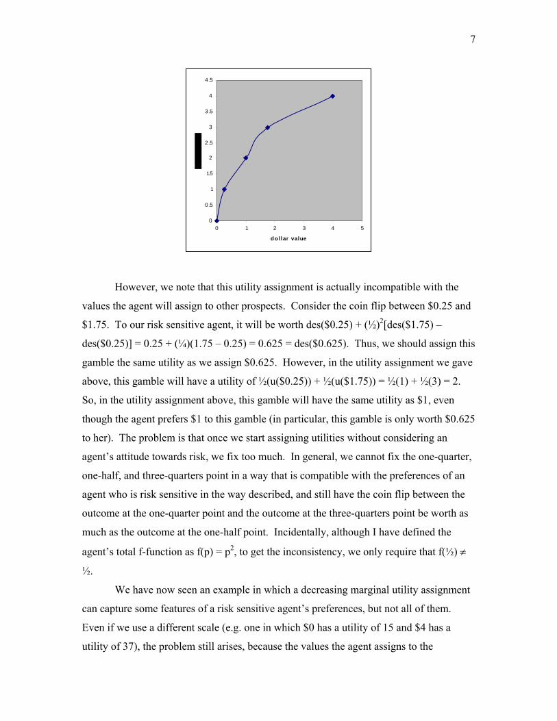
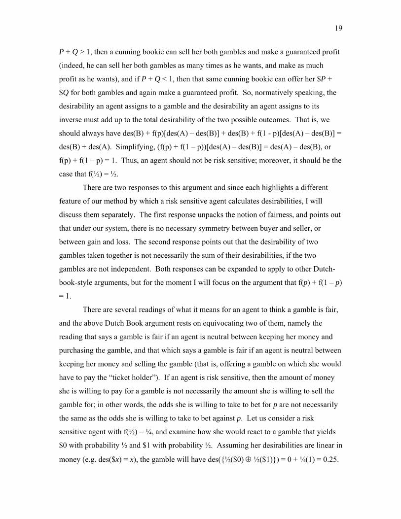
assignment of, say, 0 to $0, 1 to $0.25, 2 to $1, 3 to $1.75 and 4 to $4. In fact, this is

exactly the type of utility assignment we would expect for an agent whose preferences

over money exhibit diminishing marginal utility. Connecting these five points in a

smooth curve, her utility graph might look something like this:

v Strictly speaking, the utility she assigns to $1 falls halfway between the utility she assigns to $0 and $4, and the utility she assigns to $0.25 falls halfway between the utility she assigns to $0 and $1, but for ease of exposition and without loss of generality I am assuming that $0 has a utility of 0. Assigning some other arbitrary utility to $0 will not affect the calculations or the existence of the problem.

7

0

0.5

1

1.5

2

2.5

3

3.5

4

4.5

0 1 2 3 4 5

d o llar value

However, we note that this utility assignment is actually incompatible with the

values the agent will assign to other prospects. Consider the coin flip between $0.25 and

$1.75. To our risk sensitive agent, it will be worth des($0.25) + (½)2[des($1.75) –

des($0.25)] = 0.25 + (¼)(1.75 – 0.25) = 0.625 = des($0.625). Thus, we should assign this

gamble the same utility as we assign $0.625. However, in the utility assignment we gave

above, this gamble will have a utility of ½(u($0.25)) + ½(u($1.75)) = ½(1) + ½(3) = 2.

So, in the utility assignment above, this gamble will have the same utility as $1, even

though the agent prefers $1 to this gamble (in particular, this gamble is only worth $0.625

to her). The problem is that once we start assigning utilities without considering an

agent’s attitude towards risk, we fix too much. In general, we cannot fix the one-quarter,

one-half, and three-quarters point in a way that is compatible with the preferences of an

agent who is risk sensitive in the way described, and still have the coin flip between the

outcome at the one-quarter point and the outcome at the three-quarters point be worth as

much as the outcome at the one-half point. Incidentally, although I have defined the

agent’s total f-function as f(p) = p2, to get the inconsistency, we only require that f(½) ≠

½.

We have now seen an example in which a decreasing marginal utility assignment

can capture some features of a risk sensitive agent’s preferences, but not all of them.

Even if we use a different scale (e.g. one in which $0 has a utility of 15 and $4 has a

utility of 37), the problem still arises, because the values the agent assigns to the

8

aforementioned gambles fix the dollar amounts that must correspond to the one-quarter

point, halfway point, and three-quarters point on the scale. So we see that once we are

assigning utilities to gambles, we have already made the assumption that agents are not

risk sensitive.

Now, a question arises about when exactly the assumption of risk insensitivity

comes into play in decision theory. In particular, we want to examine the extent to which

the process of establishing utilities, using the Representation Theorem, relies on the

assumption that people are not risk sensitive. After all, if the assumption is not that

crucial, or comes into play late in the game, then it may not be too difficult to account for

risk sensitive people. And if the assumption is crucial to the process and generally not

true of people, then it seems that decision theory should be extremely bad at describing

people’s preferences. And while we have evidence that the assumption is false in

“fringe” cases (one of which I will discuss later), no one protests that a standard utility

function is way off the mark.

We will see that the assumption comes into play in the early stages of the process

– in particular, in how an agent’s desirability scale is calibrated – but that the resulting

utility function is actually similar enough to the utility function of a risk averse agent (in

the diminishing marginal utility function sense) to make the differences only apparent in

certain cases. In other words, although the assumption is crucial to the process by which

utilities are extracted from preferences, the behavior of risk sensitive people does not

diverge widely from the behavior that the Representation Theorem predicts except in a

certain set of cases – though in these cases, it diverges very widely. Thus, even if it turns

out that the assumption is false for most people, the process of the Representation

Theorem produces results that are not far off the mark in many cases, and thus results that

(taken modulo experimental error) would not immediately reveal gross inadequacies in

classical decision theory. So we have a sneaky problem: the effects of the assumption are

not immediately noticeable, but the assumption leads to a host of problems in predicting

behavior.

In order to see how crucial the assumption is, let us go through the process by

which we use the Representation Theorem to take in ordinal preferences and output

9

cardinal utilities. vi This is called the Ramsey method. The first step in the process is

calibrating the desirability scale. Choosing two conditions A and B, such that B is

preferred to A, Ramsey “finds an ethically neutral condition N which has a probability of

½ and identifies the midpoint of the scale as the estimated desirability of the gamble {A if

N, B if not}.”vii The ethically neutral condition is any condition such that the agent is

indifferent between {B if N, A if not} and {A if N, B if not}, and thus any condition that

has subjective probability ½.viii Note that N is chosen in such a way that it will still have

probability ½ if the agent is risk sensitive: both {B if N, A if not} and {A if N, B if not}

will have a lower desirability than they will for a risk insensitive agent, but they will be

equal just in case the probability of N is equal to the probability of ~N, and therefore just

in case the subjective probability of N is ½. So far the process is not affected by the risk

sensitivity of an agent; the chosen condition will meet the requirements of ethical

neutrality regardless.

Once the ethically neutral condition is chosen, we identify three points on the

scale: a point A on the lower end of the scale, a point B on the higher end of the scale,

and the point which corresponds to the desirability of {A if N, B if not} – that is,

{½A⊕½B} – as the midpoint of the scale. For a risk insensitive agent, this is an accurate

representation of how he feels about the gamble; he will actually desire B twice as much

as the gamble, where A is the default option. For a risk sensitive agent, this midpoint will

not correspond to how she actually feels about the gamble; if, for example, an agent has a

probability weighting function with f(½) = ¼ (like our earlier agent), then she would

actually place this “midpoint” only one-quarter of the way up the scale.ix Thus the

Ramsey method will make the gamble appear more desirable than it is. Of course, the

scale does not yet correspond to anything, so the fact that it is not “to scale,” so to speak,

may be irrelevant to whether the resulting utility function will actually represent the

vi Jeffrey, Richard C. The Logic of Decision, second edition. Chicago: The University of Chicago Press, 1983. Pg, 41 – 58. vii Jeffrey, 49. viii Note the further constraint that the condition is independent from A and B. The exact way in which this is spelled out is not relevant to our discussion. ix If A and B are consequences such that B is preferred to A, then the desirability of C = ½B ⊕ ½A will be des(A) + f(½)[des(B) – des(A)] = des(A) + (¼)[des(B) – des(A)]. This is ¼ when des(A) = 0 and des(B) = 1. Furthermore, she would actually place the ‘midpoint’ of A and C only one-sixteenth of the way up the scale, or one-fourth of the way between A and C.

10

preferences of the agent. So at the moment all we have is an aesthetic failing of the

procedure when it is applied to risk sensitive agents.

The next step in the process is finding a sure-thing amount C such that the agent is

indifferent between C and the gamble {A if N, B if not}. This prospect has the same

desirability as {A if N, B if not}, and thus is also placed at the midpoint of the scale. For

our agent in question, the gamble {$0 if N, $4 if not} will be worth $1, so $1 will be

placed on the midpoint of the scale, even though she will intuitively think that $1 is only

one-quarter as desirable as $4. After this, the process is repeated on each half of the

scale: the gambles {A if N, C if not} and {C if N, B if not} are placed at the one-quarter

and three-quarters points on the scale, respectively, and sure-thing amounts D and E are

chosen such that the agent is indifferent between {A if N, C if not} and D and between

{C if N, B if not} and E. And so it goes with each successive division of the desirability

scale. We then assign (arbitrary)x utility values to the upper and lower endpoint of the

scale, and calculate the utility values of the plotted points accordingly, so that the scale

just described is linear.

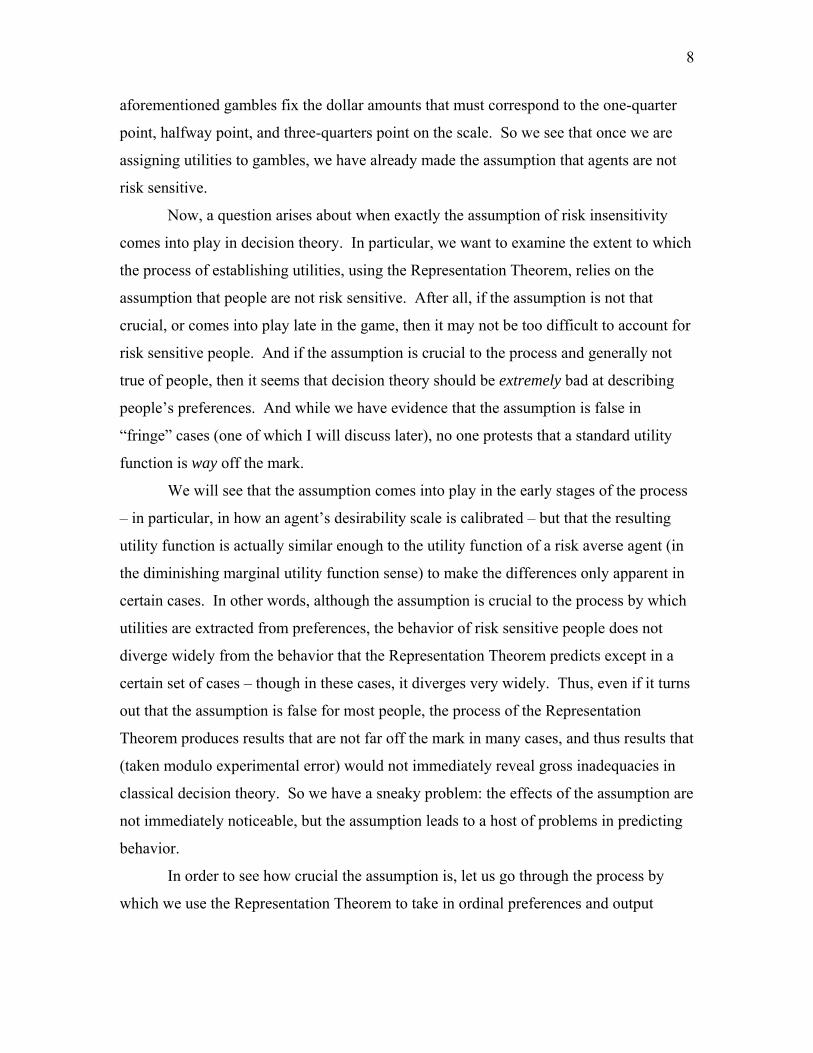
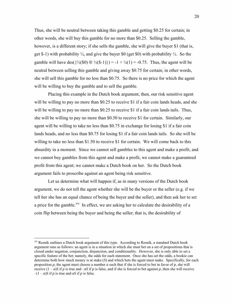
Let us see what would result for our sample risk sensitive agent. Going through

the process laid out above, we place $0 at the bottom of the scale with a utility value of 0,

and $4 at the top of the scale with utility 4. We then find an ethically neutral condition N,

discover that the agent is indifferent between {$0 if N, $4 if not} and $1, and

consequently we place $1 at the midpoint of the scale, thus assigning to $1 a utility value

of 2. Similarly, we find she is indifferent between {$0 if N, $1 if not} and $0.25, so we

place $0.25 at the midpoint of the lower interval, assigning to it a utility value of 1;

likewise we place $1.75 at the midpoint of the upper interval with utility value 3. And so

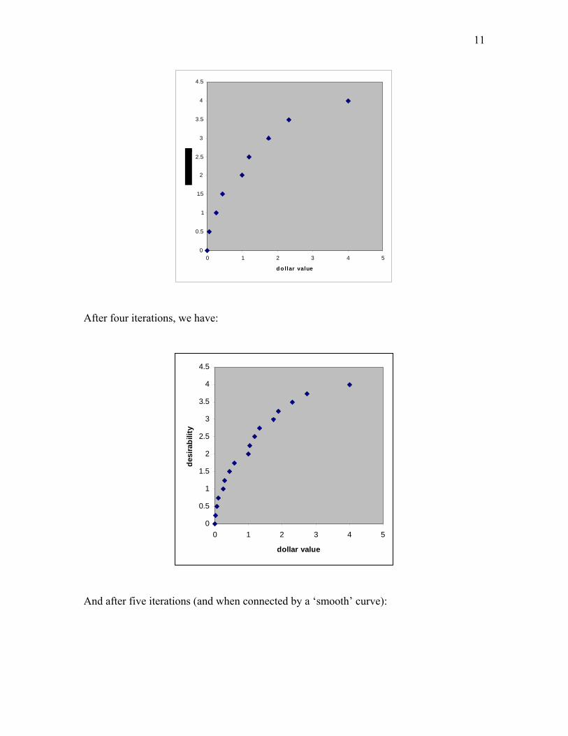
on. After three iterations of this process, we have the following utility assignment:

x In Ramsey’s theory, this assignment must be unique up to linear transformation. In Jeffrey’s theory, this is somewhat more complicated, but beyond the scope of this paper.

11

0

0.5

1

1.5

2

2.5

3

3.5

4

4.5

0 1 2 3 4 5

d o llar value

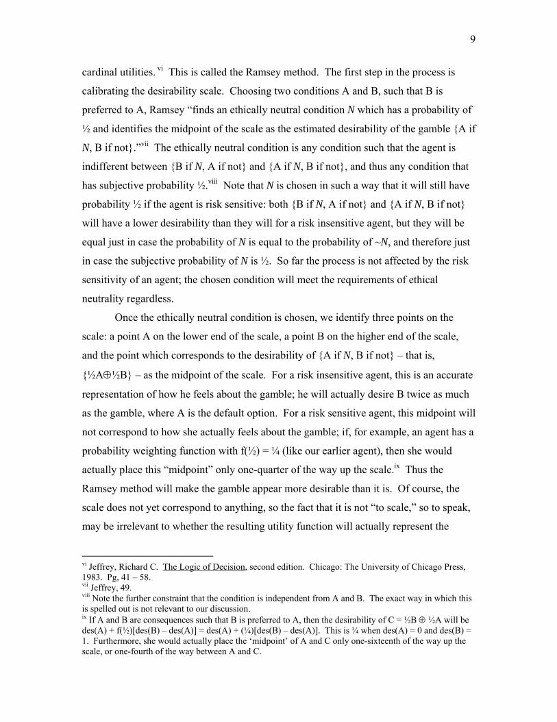
After four iterations, we have:

0

0.5

1

1.5

2

2.5

3

3.5

4

4.5

0 1 2 3 4 5

dollar value

desi

rabi

lity

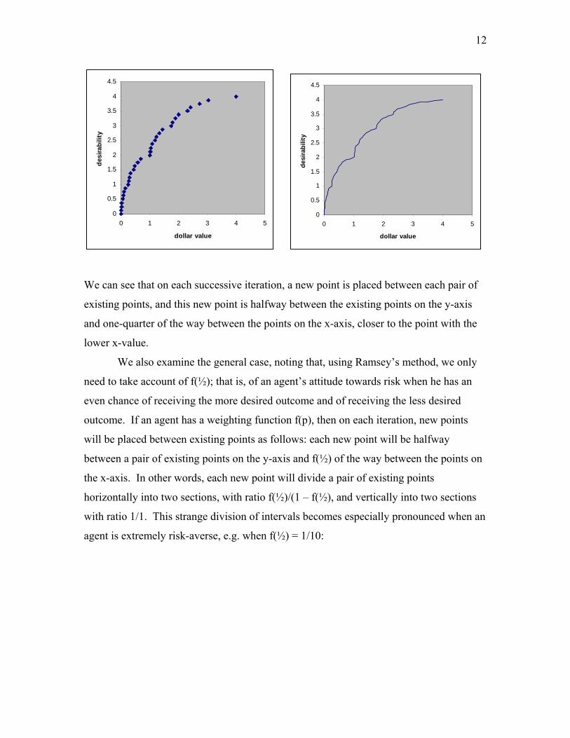
And after five iterations (and when connected by a ‘smooth’ curve):

12

0

0.5

1

1.5

2

2.5

3

3.5

4

4.5

0 1 2 3 4 5

dollar value

desi

rabi

lity

0

0.5

1

1.5

2

2.5

3

3.5

4

4.5

0 1 2 3 4 5

dollar value

desi

rabi

lity

We can see that on each successive iteration, a new point is placed between each pair of

existing points, and this new point is halfway between the existing points on the y-axis

and one-quarter of the way between the points on the x-axis, closer to the point with the

lower x-value.

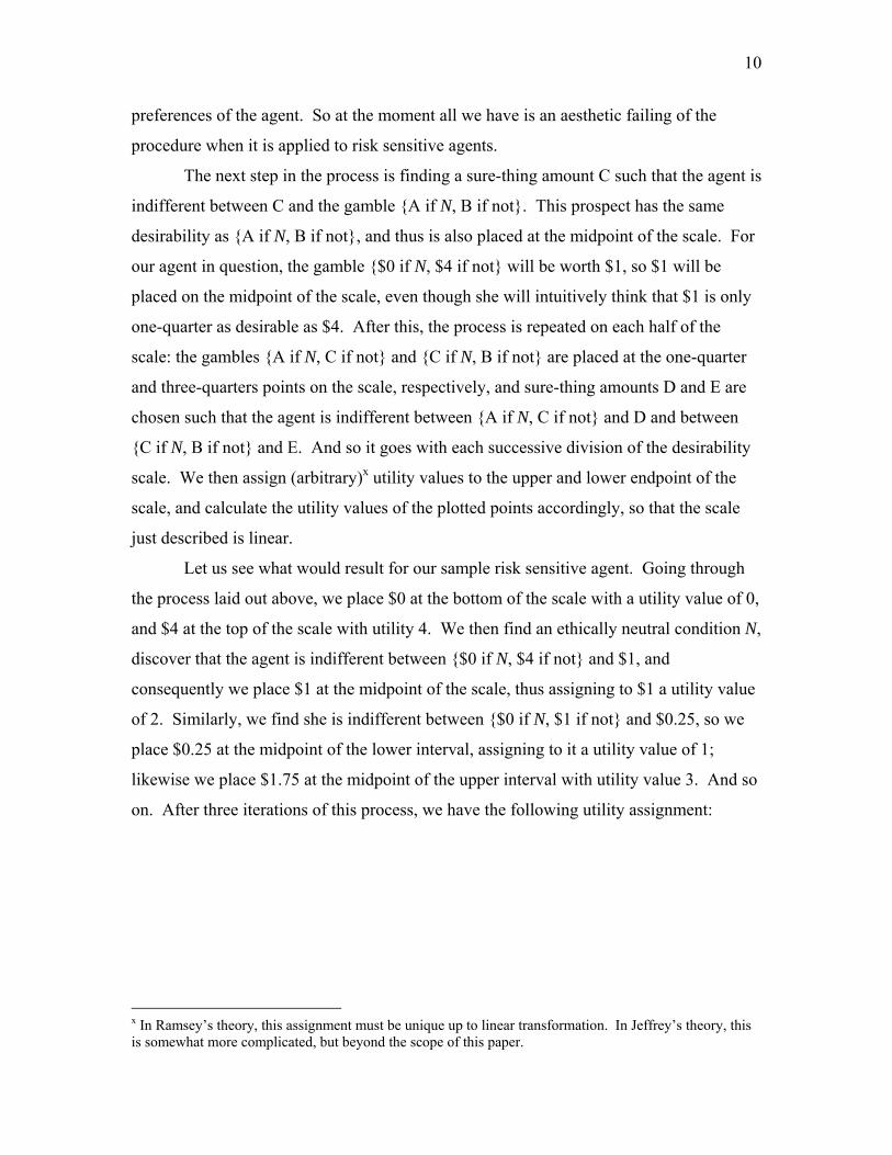
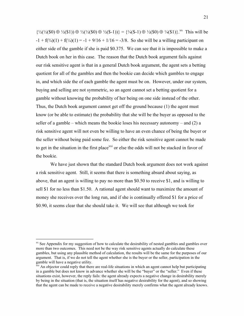
We also examine the general case, noting that, using Ramsey’s method, we only

need to take account of f(½); that is, of an agent’s attitude towards risk when he has an

even chance of receiving the more desired outcome and of receiving the less desired

outcome. If an agent has a weighting function f(p), then on each iteration, new points

will be placed between existing points as follows: each new point will be halfway

between a pair of existing points on the y-axis and f(½) of the way between the points on

the x-axis. In other words, each new point will divide a pair of existing points

horizontally into two sections, with ratio f(½)/(1 – f(½), and vertically into two sections

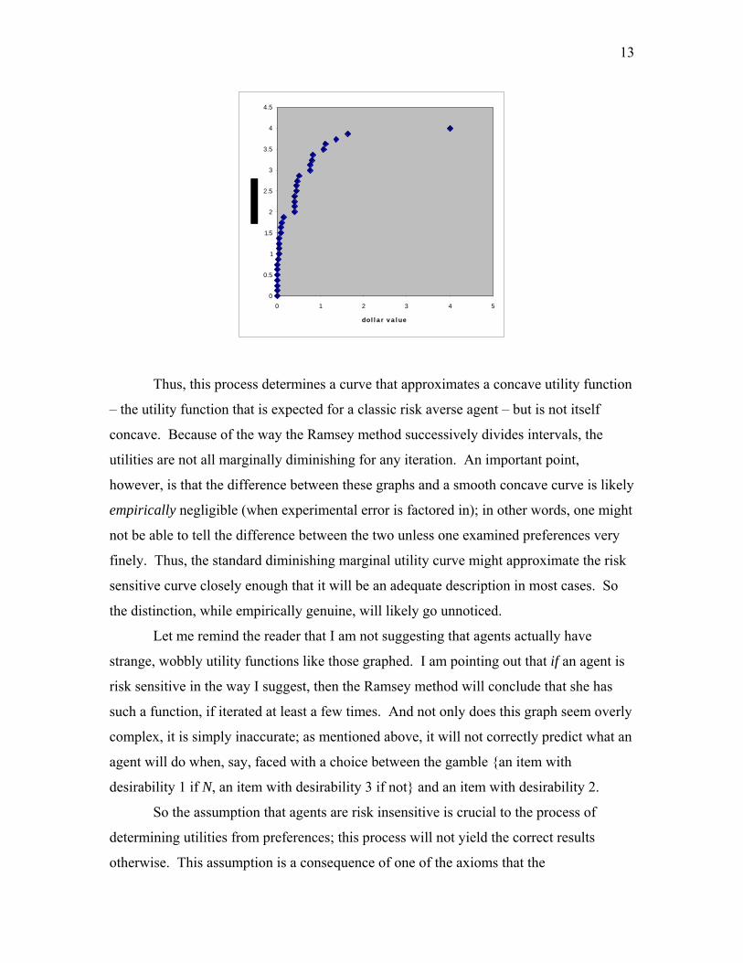
with ratio 1/1. This strange division of intervals becomes especially pronounced when an

agent is extremely risk-averse, e.g. when f(½) = 1/10:

13

0

0.5

1

1.5

2

2.5

3

3.5

4

4.5

0 1 2 3 4 5

dol l a r v a l ue

Thus, this process determines a curve that approximates a concave utility function

– the utility function that is expected for a classic risk averse agent – but is not itself

concave. Because of the way the Ramsey method successively divides intervals, the

utilities are not all marginally diminishing for any iteration. An important point,

however, is that the difference between these graphs and a smooth concave curve is likely

empirically negligible (when experimental error is factored in); in other words, one might

not be able to tell the difference between the two unless one examined preferences very

finely. Thus, the standard diminishing marginal utility curve might approximate the risk

sensitive curve closely enough that it will be an adequate description in most cases. So

the distinction, while empirically genuine, will likely go unnoticed.

Let me remind the reader that I am not suggesting that agents actually have

strange, wobbly utility functions like those graphed. I am pointing out that if an agent is

risk sensitive in the way I suggest, then the Ramsey method will conclude that she has

such a function, if iterated at least a few times. And not only does this graph seem overly

complex, it is simply inaccurate; as mentioned above, it will not correctly predict what an

agent will do when, say, faced with a choice between the gamble {an item with

desirability 1 if N, an item with desirability 3 if not} and an item with desirability 2.

So the assumption that agents are risk insensitive is crucial to the process of

determining utilities from preferences; this process will not yield the correct results

otherwise. This assumption is a consequence of one of the axioms that the

14

Representation Theorem assumes, often called the “axiom of better prizes” or the “sure

thing principle.” This axiom states that if two gambles yield the same prize for a given

result of the gambling mechanism, then a comparison of the other prizes will reveal the

agent’s preference between the gambles; she will prefer one gamble to another if and

only if she prefers the prize that gamble yields on the non-identical outcomes. More

formally,xi (x)(y)(z)(p)(xRy ↔ L[p, z, x] R L[p, z, y]), where R is the “no worse than”

relation and L[p, z, x] is a lottery that yields z with probability p and x with probability 1

– p. As a result of this axiom, only the “local” features of gambles – the absolute

desirabilities of the possible prizes – are taken into account when an agent is evaluating

gambles. Global features of gambles, such as how the overall desirability of a gamble

might be affected by the relative desirabilities of the outcomes (e.g. the intervals between

possible outcomes) and the overall probability distribution, are not taken into account.

A classic example of a situation in which people tend to violate the sure thing

principle is the Allais Paradox. I’ll use a version in which the agent receives the

following payoffs for four gambles, contingent on which ticket is randomly selected in a

100-ticket lotteryxii:

1 2-10 11-100 A $0 $500 $0 B $100 $100 $0 C $0 $500 $100 D $100 $100 $100

The majority of people presented with the choice prefer gamble A to gamble B, and

prefer gamble D to gamble C. We can show that these preferences violate the sure thing

principle. A and B yield the same prize if the ticket is between 11 and 100, so if an agent

prefers A to B, then, by the sure thing principle, the agent must prefer a 9% chance of

$500 to a 10% chance of $100.xiii However, since C and D also yield the same prize as

each other if the ticket is between 11 and 100, then, again by the principle, if an agent xi Here, I’m using James Dreier’s formulation of Michael Resnik’s version of the axiom. Dreier, “Decision Theory and Morality.” In The Oxford Handbook of Rationality, ed. Alfred R. Mele and Piers Rawling. Oxford University Press, 2004. Pg. 159. xii Broome, John. Weighing Goods. Oxford: Basil Blackwell Inc., 1991. Pg. 97. Broome uses a formulation by Savage, The Foundations of Statistics, pg. 103. Original problem Maurice Allais, “Foundations of a positive theory of choice,” pg. 89. xiii Or a 90% chance of $200 to a 100% chance of $100.

15

prefers D to C, she must prefer a 10% chance of $100 to a 9% chance of $500. An agent

cannot prefer x to y and also prefer y to x, so if the sure thing principle holds, anyone

holding the two majority preferences must be inconsistent.

On the other hand, the majority preferences on the Allais gambles are perfectly

compatible with my proposal. If A is preferred to B, then des($0) + f(.09)[des($500) –

des($0)] > des($0) + f(.1)[des($100) – des($0)], so f(.09)[des($500) – des($0)] >

f(.1)[des($100) – des($0)]. If D is preferred to C, then des($100) > des($0) +

f(.99)[des($100) – des($0)] + f(.09)[des($500) – des($100)]. These two equations do not

yield an inconsistency.xiv This highlights the point that standard decision theoretic agents

are not able to take account of global properties of gambles: in this example, gambles A

and B share local properties at tickets 11-100, as do gambles C and D. Furthermore, A

and C have the same local properties at 1-10, as do B and D. However, the gambles have

different global properties: in D, the agent wins money for sure, whereas in C, as in A

and B, it is possible that the agent will not win money. It is the presence of this global

difference in the choice between C and D that distinguishes it from the choice between A

and B. If agents evaluate risk in the way I am considering, then they do take account of

these global properties.

Let’s sum up what we have done so far. I presented an example to show that the

preferences of risk sensitive agents cannot be adequately captured by standard decision

theory with diminishing marginal utilities. I then explored what the utility function of a

risk sensitive agent might look like if we used the standard Ramsey method (and failed to

take her risk sensitivity into account): it would, after only a few iterations, look

approximately like a smooth curve with diminishing marginal utility values, but would

look much worse as the iterations progressed. Finally, I showed that risk sensitive agents

violate an axiom that is crucial to the Representation Theorem, and that this axiom makes

it impossible to take into account certain global features of prospects that risk sensitive

agents do take into account when evaluating prospects.

At this point, it seems clear that standard decision theory (with diminishing

marginal utility functions) is ill-equipped to handle the preferences of agents who are risk

xiv I will later discuss how one might deal with gambles that are over more than two options. As an example of a desirability and f-function assignment that could satisfy the conditions yielding the majority preferences, take des($0) = 0, des($100) = 100, des($500) = 500, f(0.09) = 0.09, f(0.1) = 0.1, f(0.99) = 0.5.

16

sensitive in the way I have described. If people have a probability function – or, as a

weaker condition, if they discount the expected value of coin flips at all – then because of

the way in which the method of the Representation Theorem tries to determine utility

functions from people’s preferences over gambles, we will not be able to accurately

capture their preferences. The Representation Theorem will produce a utility function

that yields the wrong results in certain cases.

There are several responses open to the defender of decision theory as an accurate

description of rational agents. First, he could claim that agents who are risk sensitive do

not have preferences that are capturable by a utility function using the Representation

Theorem because they do not have rational preferences; it is simply irrational to care

about risk in the way described. The Representation Theorem merely says that if people

have preferences that obey certain axioms, then we can capture their preferences by a

utility function that is unique up to certain transformations, and it is only meant to apply

to agents with such preferences. Still, if it turns out that many agents (even “idealized”

versions of those agentsxv) do not have such preferences, and we cannot give a

compelling reason that they should, then we have to admit that decision theory has a

limited scope. In particular, we must admit that the requirements an agent must meet in

order to count as “rational” give the term added meaning beyond what we normally use it

to mean.

Note that in claiming that my risk-sensitive agents are rational, I am doing more

than begging the question about the rationality of Allais violators; I am presenting an

intuitively plausible way in which people might process risk that explains why they

violate the Allais paradox, and why they continue to violate it even when presented with

their ‘mistake.’xvi This latter fact indicates that some agents, even upon reflection, do not

endorse the sure thing principle. Thus, the defender of the claim that Allais violators are

irrational cannot explain the paradox away by saying, e.g., that they are being tricked by

the numbers. We stated above that the axioms of decision theory are supposed to be

constitutive of rationality, and that it is incumbent on rational agents to make their

xv By an idealized agent, I mean the agent in a clear frame of mind, with perfect mathematical knowledge, etc. I do not necessarily mean the version of the agent who follows all the axioms including the sure thing principle. xvi According to Broome, Allais himself thought that the majority preferences are rational. Broome, 97.

17

preferences comply with the axioms of decision theory. If there is no good argument that

the sure thing principle is constitutive of rationality – or that agents should not be risk

sensitive – then it is hard to see why an agent who is not initially inclined to subscribe to

it should change his mind.

In the next section, I will address the normative question of whether or not risk

sensitive agents should necessarily count as irrational; that is, whether or not agents have

non-question-begging reasons to be risk insensitive. It suffices to say that the onus is on

the defender of the sure thing principle to show that it is a rational requirement. For now,

however, let us consider a potential avenue by which decision theory could accommodate

risk sensitive agents without renouncing any of its axioms.

An obvious response by classical decision theory is to push for a more fine-

grained distinction of the outcomes, as has been suggested, e.g. by John Broome, when

dealing with the Allais Paradoxxvii. It is not that agents assign values to outcomes and

then discount the values of outcomes that they will not get for certain, this approach

argues, but that what they assign values to includes not just the final outcomes but the

story of how the agents received those outcomes. For example, one might prefer a sure-

thing $100 to $100 that was received as the result of a coin flip; that is, one might prefer

$100 when she couldn’t have gotten anything else to $100 when she was in danger of

getting $0 (i.e. $100 with a negative feeling). Speaking more generally, risk sensitive

people have preferences over <outcome, probability> pairs.

Unfortunately, this response renders the method of the Representation Theorem

useless in principle for representing people’s preferences over such pairs. We cannot, for

example, ask an agent how she feels about the gamble {$0 as the result of a sure-thing

gamble if a fair coin lands heads, $100 as the result of a gamble that yields $100 25% of

the time if not}. The most we can tell from where an agent ranks a coin-flip gamble in

her preference ordering is how she feels about an outcome resulting from a gamble that

yields that outcome 50% of the time. Another way of stating this is that the story of how

an agent received an outcome is already built into the method by which one determines

an agent’s preferences over outcomes.

xvii Broome, 98-100.

18

We have now shown that there is an intuitively plausible way that agents might

take risk into account that is not capturable by classical decision theory. If an agent

really does discount the value of gambles in a way that is related to the size of the

intervals between possible outcomes – e.g. if an agent really does have an f-function –

then, according to classical decision theory, her preferences are incoherent. Therefore, it

seems that agents can have incoherent preferences without being irrational in any obvious

sense.

In the final section of this paper, I will address the normative question of whether

we can allow such agents to count as rational. I will examine a standard type of argument

that it is not rational to violate an axiom of decision theory, and apply it against the claim

that it can be rational to be risk sensitive. I will then show why the argument fails.

Are risk sensitive people rational?

We now turn to the question of whether an agent can be risk sensitive (and

consequently have incoherent preferences) without being irrational. Even if empirical

evidence shows that people are not generally risk insensitive, there may be normative

arguments that show that rational agents should be risk insensitive. A classic such

argument is a Dutch book argument.xviii One version of this argument runs as follows:

assume that an agent thinks it is fair to pay P dollars for a gamble that yields $1 if an

event E with (subjective) probability p happens and $0 if the event does not happen.

Now assume that the agent also thinks it is fair to pay Q dollars for a gamble that yields

$1 if an event with (subjective) probability 1 – p happens and $0 if the event does not

happen. Since any event with probability 1 – p can serve as the event over which to

gamble, she must also think it is fair to pay Q dollars for a gamble that yields $1 if event

E does not happen and $0 if event E does happen. Furthermore, since she thinks each

arrangement is fair, she also thinks that the first arrangement and the last arrangement

together are fair. Thus, she thinks it is fair to pay P + Q dollars for a gamble that yields

$1 + $0 if E obtains and $0 + $1 if E does not obtain. In other words, she thinks it is fair

to pay P + Q dollars to receive $1 for sure. So it should be the case that P + Q = 1; for if

xviii I will focus on the Dutch book argument for a specific claim, namely the claim that f(p) + f(1 – p) = 1 for all p. For a general version of this argument, see Michael Resnik’s Choices: An Introduction to Decision Theory. Minneapolis, MN: University of Minnesota Press, 1986.

19

P + Q > 1, then a cunning bookie can sell her both gambles and make a guaranteed profit

(indeed, he can sell her both gambles as many times as he wants, and make as much

profit as he wants), and if P + Q < 1, then that same cunning bookie can offer her $P +

$Q for both gambles and again make a guaranteed profit. So, normatively speaking, the

desirability an agent assigns to a gamble and the desirability an agent assigns to its

inverse must add up to the total desirability of the two possible outcomes. That is, we

should always have des(B) + f(p)[des(A) – des(B)] + des(B) + f(1 - p)[des(A) – des(B)] =

des(B) + des(A). Simplifying, (f(p) + f(1 – p))[des(A) – des(B)] = des(A) – des(B), or

f(p) + f(1 – p) = 1. Thus, an agent should not be risk sensitive; moreover, it should be the

case that f(½) = ½.

There are two responses to this argument and since each highlights a different

feature of our method by which a risk sensitive agent calculates desirabilities, I will

discuss them separately. The first response unpacks the notion of fairness, and points out

that under our system, there is no necessary symmetry between buyer and seller, or

between gain and loss. The second response points out that the desirability of two

gambles taken together is not necessarily the sum of their desirabilities, if the two

gambles are not independent. Both responses can be expanded to apply to other Dutch-

book-style arguments, but for the moment I will focus on the argument that f(p) + f(1 – p)

= 1.

There are several readings of what it means for an agent to think a gamble is fair,

and the above Dutch Book argument rests on equivocating two of them, namely the

reading that says a gamble is fair if an agent is neutral between keeping her money and

purchasing the gamble, and that which says a gamble is fair if an agent is neutral between

keeping her money and selling the gamble (that is, offering a gamble on which she would

have to pay the “ticket holder”). If an agent is risk sensitive, then the amount of money

she is willing to pay for a gamble is not necessarily the amount she is willing to sell the

gamble for; in other words, the odds she is willing to take to bet for p are not necessarily

the same as the odds she is willing to take to bet against p. Let us consider a risk

sensitive agent with f(½) = ¼, and examine how she would react to a gamble that yields

$0 with probability ½ and $1 with probability ½. Assuming her desirabilities are linear in

money (e.g. des($x) = x), the gamble will have des({½($0) ⊕ ½($1)}) = 0 + ¼(1) = 0.25.

20

Thus, she will be neutral between taking this gamble and getting $0.25 for certain; in

other words, she will buy this gamble for no more than $0.25. Selling the gamble,

however, is a different story; if she sells the gamble, she will give the buyer $1 (that is,

get $-1) with probability ½, and give the buyer $0 (get $0) with probability ½. So the

gamble will have des({½($0) ⊕ ½($-1)}) = -1 + ¼(1) = -0.75. Thus, the agent will be

neutral between selling this gamble and giving away $0.75 for certain; in other words,

she will sell this gamble for no less than $0.75. So there is no price for which the agent

will be willing to buy the gamble and to sell the gamble.

Placing this example in the Dutch book argument, then, our risk sensitive agent

will be willing to pay no more than $0.25 to receive $1 if a fair coin lands heads, and she

will be willing to pay no more than $0.25 to receive $1 if a fair coin lands tails. Thus,

she will be willing to pay no more than $0.50 to receive $1 for certain. Similarly, our

agent will be willing to take no less than $0.75 in exchange for losing $1 if a fair coin

lands heads, and no less than $0.75 for losing $1 if a fair coin lands tails. So she will be

willing to take no less than $1.50 to receive $1 for certain. We will come back to this

absurdity in a moment. Since we cannot sell gambles to this agent and make a profit, and

we cannot buy gambles from this agent and make a profit, we cannot make a guaranteed

profit from this agent; we cannot make a Dutch book on her. So the Dutch book

argument fails to proscribe against an agent being risk sensitive.

Let us determine what will happen if, as in many versions of the Dutch book

argument, we do not tell the agent whether she will be the buyer or the seller (e.g. if we

tell her she has an equal chance of being the buyer and the seller), and then ask her to set

a price for the gamble.xix In effect, we are asking her to calculate the desirability of a

coin flip between being the buyer and being the seller; that is, the desirability of

xix Resnik outlines a Dutch book argument of this type. According to Resnik, a standard Dutch book argument runs as follows: an agent is in a situation in which she must bet on a set of propositions that is closed under negation, conjunction, disjunction, and conditionality. However, she is only able to set a specific feature of the bet; namely, the odds for each statement. Once she has set the odds, a bookie can determine both how much money is at stake (S) and which bets the agent must make. Specifically, for each proposition p, the agent must choose a number a such that if she is forced to bet in favor of p, she will receive (1 – a)S if p is true and –aS if p is false, and if she is forced to bet against p, then she will receive –(1 – a)S if p is true and aS if p is false.

21

{½(½($0) ⊕ ½($1)) ⊕ ½(½($0) ⊕ ½($-1))} = {¼($-1) ⊕ ½($0) ⊕ ¼($1)}.xx This will be

-1 + f(¾)(1) + f(¼)(1) = -1 + 9/16 + 1/16 = -3/8. So she will be a willing participant on

either side of the gamble if she is paid $0.375. We can see that it is impossible to make a

Dutch book on her in this case. The reason that the Dutch book argument fails against

our risk sensitive agent is that in a general Dutch book argument, the agent sets a betting

quotient for all of the gambles and then the bookie can decide which gambles to engage

in, and which side the of each gamble the agent must be on. However, under our system,

buying and selling are not symmetric, so an agent cannot set a betting quotient for a

gamble without knowing the probability of her being on one side instead of the other.

Thus, the Dutch book argument cannot get off the ground because (1) the agent must

know (or be able to estimate) the probability that she will be the buyer as opposed to the

seller of a gamble – which means the bookie loses his necessary autonomy – and (2) a

risk sensitive agent will not even be willing to have an even chance of being the buyer or

the seller without being paid some fee. So either the risk sensitive agent cannot be made

to get in the situation in the first placexxi or else the odds will not be stacked in favor of

the bookie.

We have just shown that the standard Dutch book argument does not work against

a risk sensitive agent. Still, it seems that there is something absurd about saying, as

above, that an agent is willing to pay no more than $0.50 to receive $1, and is willing to

sell $1 for no less than $1.50. A rational agent should want to maximize the amount of

money she receives over the long run, and if she is continually offered $1 for a price of

$0.90, it seems clear that she should take it. We will see that although we took for

xx See Appendix for my suggestion of how to calculate the desirability of nested gambles and gambles over more than two outcomes. This need not be the way risk sensitive agents actually do calculate these gambles, but using any plausible method of calculation, the results will be the same for the purposes of our argument. That is, if we do not tell the agent whether she is the buyer or the seller, participation in the gamble will have a negative utility. xxi An objector could reply that there are real-life situations in which an agent cannot help but participating in a gamble but does not know in advance whether she will be the “buyer” or the “seller.” Even if these situations exist, however, the reply fails: the agent already expects a negative change in desirability merely by being in the situation (that is, the situation itself has negative desirability for the agent), and so showing that the agent can be made to receive a negative desirability merely confirms what the agent already knows.

22

granted an assumption that lead to the absurd conclusion that an agent is willing to pay no

more than $0.50 to receive $1, the assumption is false.xxii

So far we have been speaking as if the desirability of two gambles together is

simply the sum of their desirabilities. As we turn to the second response to the Dutch

book argument, we will show that this is not always the case, and that we cannot deduce

that an agent will only be willing, e.g., to pay $0.50 to receive $1 for certain. Note that

when we add two gambles, we treat the resulting gamble as a single gamble over all of

the possible outcomes, where each outcome has a simple (as opposed to compound)

probability.xxiii In general, the probability that a given outcome obtains will be a

weighted sum of its probability of obtaining in each component gamble. However, if the

outcome of one of the component gambles is contingent on the outcome of another of the

component gambles, then this will not hold. If an agent is taking a compound gamble in

which the first gamble yields $1 if an event with probability ½ obtains and $0 otherwise

and the second gamble yields $1 if an independent event with probability ½ obtains and

$0 otherwise, then the compound gamble will have the same desirability as the gamble

{¼($0) ⊕ ½($1) ⊕ ¼($2)}. Since the Dutch bookie can have no more background

information than the agent in question (save the mathematical wherewithal that makes

Dutch book arguments go through in the first place), he cannot know that the two

gambles involve the same event if the agent in question does not know. Thus, in our

example, the agent must know that the gambles are not independent. Since one gamble

yields $1 if and only if the other gamble yields $0, there are only two possible outcomes

– winning $1 from the first gamble and $0 from the second, or vice versa – and since our

agent knows this, each outcome has subjective probability ½. In either case the agent

will receive $1, so the desirability of the ‘gamble’ which yields $1 if E obtains and $1 if

E does not obtain is des($1) + f(p)[des($1) – des($1)] = des($1). Thus, receiving $1 for

xxii Note that undermining the assumption will not undermine our original reply to the Dutch book argument; we have already shown that even if the assumption is true, then the Dutch book argument fails. We will now show that it fails for even stronger reasons; namely, that a certain independence assumption is false. xxiii See discussion in Appendix.

23

certain will have exactly the desirability that $1 has. xxiv In other words, the compound

gamble in our example has the same desirability as the gamble {½($1) ⊕ ½($1)} ≈ $1.

This second reply highlights an interesting feature of our system: the worth of two

gambles with overlapping outcomes or events by which outcomes are determined is not

merely the worth of one gamble plus the worth of the other. This fits with our intuitions

about how gambles relate to each other; after all, the outcome that obtains in a certain

gamble may affect how much an agent values the various results of subsequent

gambles.xxv

One final point on the part of the defender of the claim that risk sensitive agents

are necessarily irrational: perhaps we cannot make a Dutch book against risk sensitive

agents, but it still appears that they will do worse in the long run, and even fail to satisfy

their own long-run preferences. After all, risk sensitive people will make less money –

or, more precisely, will gain less utility – in the long run than those who don’t. If an

agent is not willing to pay $0.40 each for a string of coin flips that yield either $0 or $1,

chances are she will end up with less in the long run than an agent who is. Since global

properties “wash out” in the long run, everything that is relevant to maximizing long-run

utility is already accounted for in the local properties of a gamble. And even if an agent

is only engaging in a gamble once, she should act so as to maximize long-run utility,

since expected utility more or less is long-run utility.

To respond to this objection, we first note that if an agent is engaging in the a

gamble only once, it is unclear why she should act so as to maximize the utility she would

get if she were to engage in them many times.xxvi Next, we note that if an agent knows

she is going to take the gambles, say, 100 times, her expected utility changes. On my

proposal, the utility of gambles may be different if an agent plans to take them multiple

times, since taking gambles multiple times changes the probabilities of getting the

outcomes. For example, assume that an agent is offered a gamble that gives her $100 if a

fair coin lands heads and $0 if it lands tails. The probability of it landing heads in one

trial is ½, so the value of the gamble to the agent will depend on her value of f(½). Now xxiv Note the similarity to the point in the previous section about the gamble between the 2003 dollar bill and the 2004 dollar bill. xxv See the discussion of framing effects in Kahneman and Tversky, pg. 286. xxvi For an interesting discussion of this point, see Putnam, Hilary. “Rationality in Decision Theory and Ethics.” Critica 18 (1988), pg 3-16.

24

assume she is offered a sequence of 10 such gambles (i.e. that same gamble 10 times in a

row). This is no longer a gamble with two possible outcomes; rather, it is a gamble with

11 possible outcomes. The probability of the coin landing heads zero times (which will

yield $0) is 1/210, the probability of the coin landing heads one time (which will yield

$100) is 10/210, etc. She has a fairly high probability of receiving between $400 and

$600, and thus, unless she is extremely risk sensitive, the gamble will be worth

somewhere between $400 and $500. Note that the value of this sequence of gambles to

the agent will depend on her value of f(1/210), f(10/210), etc. Of course, this response

does assume that the agent knows – or can estimate – the number of gambles she will be

offered. This assumption may be debated, but that is beyond the scope of this paper; we

should note, in its favor, that it mirrors the assumption that Dutch bookies cannot know

more than the agent they are interacting with.

To conclude this section, I should note that a defender of the sure-thing principle

might be convinced that we cannot make a Dutch book on my risk sensitive agents, and

yet still maintain that they are irrational. She might claim that we do not need arguments

to show that the sure-thing principle is a rational requirement; it is just obvious. As a

reply, I can only offer that the positive part of this project – exploring how we might

represent risk-sensitive agents – has interest even for those who think that the sure-thing

principle is a rational requirement: it is informative to see exactly why decision theory

fails for a certain sort of irrational agent, and it is useful to have a possible method of

representing the preferences of these agents.

Conclusion

In this paper, I have argued that there is a type of rational agent whose preferences

are intuitively plausible but incoherent on the standard decision theoretic framework. I

have given several examples to show that decision theory will give the wrong predictions

for these risk sensitive agents in certain cases, and I have pointed out that the Ramsey

method, when applied coarsely, will not distinguish risk sensitive agents from agents with

diminishing marginal utility functions, even though there is an empirical difference

between the two. I showed that there is a certain axiom that risk sensitive agents violate,

and argued that there are no non-question-begging reasons to adhere one’s preferences to

25

that axiom. I then explored an argument that purported to show that a Dutch book can be

made on a risk sensitive agent, and consequently, that such agents are irrational. This

argument failed for two reasons: first, because there is no necessary symmetry between

buying a gamble and selling that same gamble with the payoffs reversed, and second,

because the Dutch book argument in this case relies on non-independent gambles.

Finally, I briefly explored a question about how risk sensitive agents fare in the long run.

I conclude that not only is there empirical evidence that risk sensitive agents exist,

but there are also no good arguments to show that these agents violate our standard norm

of rationality. Thus, it is possible to be rational and yet have preferences that are not

capturable by standard decision theory.

26

APPENDIX: Nested Gambles and Gambles with Several Outcomes

For the section of the discussion dealing with normative arguments against being risk sensitive, it

is necessary to calculate the desirability of gambles over more than two options or of gambles over

gambles. Our formula for gambles over several options or for gambles over gambles must determine a

single desirability for each class of gambles which we consider equivalent. Now it may be unclear what is

to count as an equivalence class of gambles, and I will not attempt to give all the necessary and sufficient

conditions for two gambles being equivalent. However, I will give one sufficient condition that seems

uncontroversial: if two gambles have equal probability of yielding outcomes of equal desirability, then it

seems clear that they should have the same desirability as each other. For example, the gamble that yields

outcome A with probability ½ and yields another gamble with probability ½, which in turn yields B with

probability ½ and C with probability ½ should have the same desirability as a gamble that yields B with

probability ¼ and yields another gamble with probability 3/4 , which in turn yields A with probability 2/3

and C with probability 1/3, and both should have the same desirability as a gamble that yields A with

probability ½, B with probability ¼, and C with probability ¼. That is, the desirability of nested and

compound gambles should be independent of the order in which the gambles are carried out.

The way I’ve set up the desirability equation emphasizes that an agent considers his possible gain

above the minimum he is guaranteed (the interval between the low outcome and the high outcome), and

discounts that gain by a factor which is a function of the probability of obtaining the gain, a function that

depends on how risk sensitive he is. Analogously, when he stands to arrive at one of more than two

possible outcomes, it seems natural that he should consider the possible gain between each neighboring pair

of outcomes and his chance of arriving at the higher outcome or better. For example, consider the gamble

that yields $1 with probability ½, $2 with probability ¼, and $4 with probability ¼. The agent will get at

least $1 for certain, and he has a ½ probability of making at least $1 more. Furthermore, he has a ¼

probability of making at least $2 beyond that. So the desirability of the gamble should be des($1) +

f(½)[des($2) – des($1)] + f(¼)[des($4) – des($2)]. This method of calculating gambles is a “bottom up”

approach, in which the agent is treated as if he starts off with the worst option, and at each stage takes a

gamble to see if he moves up to a slightly better option.

There are other possible methods of calculating nested gambles that seem intuitively plausible.

One of these methods employs a “top down” approach, a sort of backwards induction from the highest

gamble. Here, the desirability of the gamble between the best two options is calculated, then the

desirability of the gamble between this gamble and the next best option is calculated, and so on until the

original gamble is treated as a gamble between the worst option and a gamble between better options.

Using the example from the previous paragraph, the desirability of the gamble between the top two options

27

is des($2) + f(½)[des($4) – des($2)]. The desirability of the gamble between the third option and this

gamble is then des($1) + f(½)[des($2) – des($1)] + f(½)f(½)[des($4) – des($2)].xxvii

The bottom up approach and the top down approach yield almost the same result. The difference

between the two is that in the top down approach, the best option is treated as the result of two gambles

instead of one. If there were more than three options, the better options would be treated as the results of

more gambles, instead of one as would happen in the bottom up approach. This seems counterintuitive to

how an agent would think about gambles; from the agent’s point of view, the results of all of the gambles

may as well be determined simultaneously. I do not have room here to further discuss the merits of the two

approaches or to further defend my proposal for how to think about gambles over several outcomes, but it

suffices to say that I think the top down approach overcomplicates an agent’s treatment of gambles, and

that the bottom up approach follows most naturally from our focus on the size of the interval between two

outcomes.xxviii In any case, this is mostly speculation on how to calculate more complex gambles than

those I deal with in the bulk of my paper.

xxvii To arrive at this, we noted that the desirability of the gamble between on the one hand the third option and on the other hand the gamble between the top two options is des($1) + f(½)[(des($2) + f(½)[des($4) – des($2)] – des($1)]. xxviii The two approaches amount to the same thing if f(a)f(b) = f(ab). Whether this is a reasonable constraint for an agent’s probability function is beyond the scope of this paper.

28

WORKS CITED

Broome, John. Weighing Goods. Oxford: Basil Blackwell Inc., 1991. Dreier, James. “Decision Theory and Morality.” In The Oxford Handbook of Rationality,

ed. Alfred R. Mele and Piers Rawling. Oxford University Press, 2004. Jeffrey, Richard C. The Logic of Decision, second edition. Chicago: The University of

Chicago Press, 1983. Kahneman, Daniel and Tversky, Amos. “Prospect Theory: An Analysis of Decision

under Risk.” Econometrica, Vol. 42, No. 2 (March 1979). Putnam, Hilary. “Rationality in Decision Theory and Ethics.” Critica 18 (1988). Resnik, Michael. Choices: An Introduction to Decision Theory. Minneapolis, MN:

University of Minnesota Press, 1986