arX

iv:1

105.

6154

v1 [

stat

.ME

] 3

1 M

ay 2

011

CONDITIONAL QUANTILE PROCESSES BASED ON SERIES OR MANY

REGRESSORS

ALEXANDRE BELLONI, VICTOR CHERNOZHUKOV AND IVAN FERNANDEZ-VAL

Abstract. Quantile regression (QR) is a principal regression method for analyzing the

impact of covariates on outcomes. The impact is described by the conditional quantile

function and its functionals. In this paper we develop the nonparametric QR series frame-

work, covering many regressors as a special case, for performing inference on the entire

conditional quantile function and its linear functionals. In this framework, we approxi-

mate the entire conditional quantile function by a linear combination of series terms with

quantile-specific coefficients and estimate the function-valued coefficients from the data.

We develop large sample theory for the empirical QR coefficient process, namely we ob-

tain uniform strong approximations to the empirical QR coefficient process by conditionally

pivotal and Gaussian processes, as well as by gradient and weighted bootstrap processes.

We apply these results to obtain estimation and inference methods for linear function-

als of the conditional quantile function, such as the conditional quantile function itself, its

partial derivatives, average partial derivatives, and conditional average partial derivatives.

Specifically, we obtain uniform rates of convergence, large sample distributions, and infer-

ence methods based on strong pivotal and Gaussian approximations and on gradient and

weighted bootstraps. All of the above results are for function-valued parameters, holding

uniformly in both the quantile index and in the covariate value, and covering the pointwise

case as a by-product. If the function of interest is monotone, we show how to use mono-

tonization procedures to improve estimation and inference. We demonstrate the practical

utility of these results with an empirical example, where we estimate the price elasticity

function of the individual demand for gasoline, as indexed by the individual unobserved

propensity for gasoline consumption.

Keywords. Quantile regression series processes, uniform inference.

JEL Subject Classification. C12, C13, C14.

AMS Subject Classification. 62G05, 62G15, 62G32.

Date: first version May, 2006, this version of June 5, 2018. The main results of this paper, particularly the pivotal

method for inference based on the entire quantile regression process, were first presented at the NAWM Econometric Society,

New Orleans, January, 2008 and also at the Stats in the Chateau in September 2009. We are grateful to Arun Chandraksekhar,

Denis Chetverikov, Ye Luo, Denis Tkachenko, and Sami Stouli for careful readings of several versions of the paper. We thank

Andrew Chesher, Roger Koenker, Oliver Linton, Tatiana Komarova, and seminar participants at the Econometric Society

meeting, CEMMAP master-class, Stats in the Chateau, BU, Duke, and MIT for many useful suggestions. We gratefully

acknowledge research support from the NSF.

1

2

1. Introduction

Quantile regression (QR) is a principal regression method for analyzing the impact of

covariates on outcomes, particularly when the impact might be heterogeneous. This impact

is characterized by the conditional quantile function and its functionals [3, 7, 24]. For exam-

ple, we can model the log of the individual demand for some good, Y , as a function of the

price of the good, the income of the individual, and other observed individual characteristics

X and an unobserved preference U for consuming the good, as

Y = Q(X,U),

where the function Q is strictly increasing in the unobservable U . With the normalization

that U ∼ Uniform(0, 1) and the assumption that U and X are independent, the function

Q(X,u) is the u-th conditional quantile of Y given X, i.e. Q(X,u) = QY |X(u|X). This

function can be used for policy analysis. For example, we can determine how changes in

taxes for the good could impact demand heterogeneously across individuals.

In this paper we develop the nonparametric QR series framework for performing inference

on the entire conditional quantile function and its linear functionals. In this framework,

we approximate the entire conditional quantile function QY |X(u|x) by a linear combination

of series terms, Z(x)′β(u). The vector Z(x) includes transformations of x that have good

approximation properties such as powers, trigonometrics, local polynomials, or B-splines.

The function u 7→ β(u) contains quantile-specific coefficients that can be estimated from

the data using the QR estimator of Koenker and Bassett [25]. As the number of series

terms grows, the approximation error QY |X(u|x) − Z(x)′β(u) decreases, approaching zero

in the limit. By controlling the growth of the number of terms, we can obtain consistent

estimators and perform inference on the entire conditional quantile function and its linear

functionals. The QR series framework also covers as a special case the so called many

regressors model, which is motivated by many new types of data that emerge in the new

information age, such as scanner and online shopping data.

We describe now the main results in more detail. Let β(·) denote the QR estimator of

β(·). The first set of results provides large-sample theory for the empirical QR coefficient

process of increasing dimension√n(β(·)−β(·)). We obtain uniform strong approximations

to this process by a sequence of the following stochastic processes of increasing dimension:

(i) a conditionally pivotal process,

(ii) a gradient bootstrap process,

3

(iii) a Gaussian process, and

(iv) a weighted bootstrap process.

To the best of our knowledge, all of the above results are new. The existence of the pivotal

approximation emerges from the special nature of QR, where a (sub) gradient of the sam-

ple objective function evaluated at the truth is pivotal conditional on the regressors. This

allows us to perform high-quality inference without even resorting to Gaussian approxima-

tions. We also show that the gradient bootstrap, introduced by Parzen, Wei and Ying [30]

in the parametric context, is effectively a means of carrying out the conditionally pivotal

approximation without explicitly estimating Jacobian matrices. The conditions for validity

of these two schemes require only a mild restriction on the growth of the number of series

terms in relation to the sample size. We also obtain a Gaussian approximation to the entire

distribution of QR process of increasing dimension by using chaining arguments and Yurin-

skii’s coupling. Moreover, we show that the weighted bootstrap works to approximate the

distribution of QR process for the same reason as the Gaussian approximation. The condi-

tions for validity of the Gaussian and weighted bootstrap approximations, however, appear

to be substantively stronger than for the pivotal and gradient bootstrap approximations.

The second set of results provides estimation and inference methods for linear functionals

of the conditional quantile function, including

(i) the conditional quantile function itself, (u, x) 7→ QY |X(u|x),(ii) the partial derivative function, (u, x) 7→ ∂xk

QY |X(u|x),(iii) the average partial derivative function, u 7→

∫∂xk

QY |X(u|x)dµ(x), and(iv) the conditional average partial derivative, (u, xk) 7→

∫∂xk

QY |X(u|x)dµ(x|xk),

where µ is a given measure and xk is the k-th component of x. Specifically, we derive uni-

form rates of convergence, large sample distributions and inference methods based on the

strong pivotal and Gaussian approximations and on the gradient and weighted bootstraps.

It is noteworthy that all of the above results apply to function-valued parameters, holding

uniformly in both the quantile index and the covariate value, and covering pointwise nor-

mality and rate results as a special case. If the function of interest is monotone, we show

how to use monotonization procedures to improve estimation and inference.

The paper contributes and builds on the existing important literature on conditional

quantile estimation. First and foremost, we build on the work of He and Shao [22] that

studied the many regressors model and gave pointwise limit theorems for the QR estimator

in the case of a single quantile index. We go beyond the many regressors model to the series

4

model and develop large sample estimation and inference results for the entire QR process.

We also develop analogous estimation and inference results for the conditional quantile

function and its linear functionals, such as derivatives, average derivatives, conditional

average derivatives, and others. None of these results were available in the previous work.

We also build on Lee [28] that studied QR estimation of partially linear models in the

series framework for a single quantile index, and on Horowitz and Lee [23] that studied

nonparametric QR estimation of additive quantile models for a single quantile index in a

series framework. Our framework covers these partially linear models and additive models

as important special cases, and allows us to perform inference on a considerably richer set

of functionals, uniformly across covariate values and a continuum of quantile indices. Other

very important work includes Chaudhuri [10], and Chaudhuri, Doksum and Samarov [11],

Hardle, Ritov, and Song [20], Cattaneo, Crump, and Jansson [8], and Kong, Linton, and

Xia [27], among others, but this work focused on local, non-series, methods.

Our work also relies on the series literature, at least in a motivational and conceptual

sense. In particular, we rely on the work of Stone [35], Andrews [2], Newey [29], Chen

and Shen [13], Chen [12] and others that rigorously motivated the series framework as an

approximation scheme and gave pointwise normality results for least squares estimators,

and on Chen [12] and van de Geer [36] that gave (non-uniform) consistency and rate results

for general series estimators, including quantile regression for the case of a single quantile

index. White [38] established non-uniform consistency of nonparametric estimators of the

conditional quantile function based on a nonlinear series approximation using artificial neu-

ral networks. In contrast to the previous results, our rate results are uniform in covariate

values and quantile indices, and cover both the quantile function and its functionals. More-

over, we not only provide estimation rate results, but also derive a full set of results on

feasible inference based on the entire quantile regression process.

While relying on previous work for motivation, our results require to develop both new

proof techniques and new approaches to inference. In particular, our proof techniques

rely on new maximal inequalities for function classes with growing moments and uniform

entropy. One of our inference approaches involves an approximation to the entire conditional

quantile process by a conditionally pivotal process, which is not Donsker in general, but

can be used for high-quality inference. The utility of this new technique is particularly

apparent in our high-dimensional setting. Under stronger conditions, we also establish an

asymptotically valid approximation to the quantile regression process by Gaussian processes

using Yurinskii’s coupling. Previously, [15] used Yurinskii’s coupling to obtain a strong

5

approximation to the least squares series estimator. The use of this technique in our context

is new and much more involved, because we approximate an entire empirical QR process of

an increasing dimension, instead of a vector of increasing dimension, by a Gaussian process.

Finally, it is noteworthy that our uniform inference results on functionals, where uniformity

is over covariate values, do not even have analogs in the least squares series literature (the

extension of our results to least squares is a subject of ongoing research, [5]).

This paper does not deal with sparse models, where there are some key series terms and

many “non-key” series terms which ideally should be omitted from estimation. In these

settings, the goal is to find and indeed remove most of the “non-key” series terms before

proceeding with estimation. [6] obtained rate results for quantile regression estimators in

this case, but did not provide inference results. Even though our paper does not explic-

itly deal with inference in sparse models after model selection, the methods and bounds

provided herein are useful for analyzing this problem. Investigating this matter rigorously

is a challenging issue, since it needs to take into account the model selection mistakes in

estimation, and is beyond the scope of the present paper; however, it is a subject of our

ongoing research.

Plan of the paper. The rest of the paper is organized as follows. In Section 2, we describe

the nonparametric QR series model and estimators. In Section 3, we derive asymptotic

theory for the series QR process. In Section 4, we give estimation and inference theory for

linear functionals of the conditional quantile function and show how to improve estimation

and inference by imposing monotonicity restrictions. In Section 5, we present an empirical

application to the demand of gasoline and a computational experiment calibrated to the

application. The computational algorithms to implement our inference methods and the

proofs of the main results are collected in the Appendices.

Notation. In what follows, Sm−1 denotes the unit sphere in Rm. For x ∈ R

m, we define

the Euclidian norm as ‖x‖ := supα∈Sm−1 |α′x|. For a set I, diam(I) = supv,v∈I ‖v − v‖denotes the diameter of I, and int(I) denotes the interior of I. For any two real numbers a

and b, a ∨ b = maxa, b and a ∧ b = mina, b. Calligraphic letters are used to denote the

support of interest of a random variable or vector. For example, U ⊂ (0, 1) is the support of

U , X ⊂ Rd is the support of X, and Z = Z(x) ∈ R

m : x ∈ X is the support of Z = Z(X).

The relation an . bn means that an ≤ Cbn for a constant C and for all n large enough.

We denote by P ∗ the probability measure induced by conditioning on any realization of

the data Dn := (Yi,Xi) : 1 ≤ i ≤ n. We say that a random variable ∆n = oP ∗(1) in

P -probability if for any positive numbers ǫ > 0 and η > 0, PP ∗(|∆n| > ǫ) > η = o(1), or

6

equivalently, P ∗(|∆n| > ǫ) = oP (1). We typically shall omit the qualifier “in P -probability.”

The operator E denotes the expectation with respect to the probability measure P , En

denotes the expectation with respect to the empirical measure, and Gn denotes√n(En−E).

2. Series Framework

2.1. The set-up. The set-up corresponds to the nonparametric QR series framework:

Y = QY |X(U |X) = Z ′β(U) +R(X,U), U |X ∼ Uniform(0, 1) and β(u) ∈ Rm,

where X is a d-vector of elementary regressors, and Z = Z(X) is an m-vector of approxi-

mating functions formed by transformations of X with the first component of Z equal to

one. The function Z ′β(u) is the series approximation to QY |X(u|X) and is linear in the

parameter vector β(u), which is defined below. The term R(X,u) is the approximation

error, with the special case of R(X,u) = 0 corresponding to the many regressors model.

We allow the series terms Z(X) to change with the sample size n, i.e. Z(X) = Zn(X), but

we shall omit the explicit index indicating the dependence on n. We refer the reader to

Newey [29] and Chen [12] for examples of series functions, including (i) regression splines,

(ii) polynomials, (iii) trigonometric series, (iv) compactly supported wavelets, and others.

Interestingly, in the latter scheme, the entire collection of series terms is dependent upon

the sample size.

For each quantile index u ∈ (0, 1), the population coefficient β(u) is defined as a solution

to

minβ∈Rm

E[ρu(Y − Z ′β)] (2.1)

where ρu(z) = (u − 1z < 0)z is the check function ([24]). Thus, this coefficient is not

a solution to an approximation problem but to a prediction problem. However, we show

in Lemma 1 in Appendix B that the solution to (2.1) inherits important approximation

properties from the best least squares approximation of QY |X(u|·) by a linear combination

of Z(·).We consider estimation of the coefficient function u 7→ β(u) using the entire quantile

regression process over U , a compact subset of (0, 1),

u 7→ β(u), u ∈ U,

7

namely, for each u ∈ U , the estimator β(u) is a solution to the empirical analog of the

population problem (2.1)

minβ∈Rm

En[ρu(Yi − Z ′iβ)]. (2.2)

We are also interested in various functionals of QY |X(·|x). We estimate them by the corre-

sponding functionals of Z(x)′β(·), such as the estimator of the entire conditional quantile

function, (x, u) 7→ Z(x)′β(u), and derivatives of this function with respect to the elementary

covariates x.

2.2. Regularity Conditions. In our framework the entire model can change with n, al-

though we shall omit the explicit indexing by n. We will use the following primitive as-

sumptions on the data generating process, as n→ ∞ and m = m(n) → ∞.

Condition S.

S.1 The data Dn = (Yi,X ′i)′, 1 ≤ i ≤ n are an i.i.d. sequence of real (1 + d)-vectors,

and Zi = Z(Xi) is a real m-vector for i = 1, . . . , n.

S.2 The conditional density of the response variable fY |X(y|x) is bounded above by f

and its derivative in y is bounded above by f ′, uniformly in the arguments y and

x ∈ X and in n; moreover, fY |X(QY |X(u|x)|x) is bounded away from zero uniformly

for all arguments u ∈ U , x ∈ X , and n.

S.3 For every m, the eigenvalues of the Gram matrix Σm = E[ZZ ′] are bounded from

above and away from zero, uniformly in n.

S.4 The norm of the series terms obeys maxi≤n ‖Zi‖ ≤ ζ(m,d, n) := ζm.

S.5 The approximation error term R(X,U) is such that supx∈X ,u∈U |R(x, u)| . m−κ.

Comment 2.1. Condition S is a simple set of sufficient conditions. Our proofs and lem-

mas gathered in the appendices hold under more general, but less primitive, conditions.

Condition S.2 impose mild smoothness assumptions on the conditional density function.

Condition S.3 and S.4 imposes plausible conditions on the design, see Newey [29]. Condi-

tion S.2 and S.3 together imply that the eigenvalues of the Jacobian matrix

Jm(u) = E[fY |X(QY |X(u|X)|X)ZZ ′]

are bounded away from zero and from above; Lemma 12 further shows that this together

with S.5 implies that the eigenvalues of Jm(u) = E[fY |X(Z ′β(u)|X)ZZ ′] are bounded away

from zero and from above, since the two matrices are uniformly close. Assumption S.4

imposes a uniform bound on the norm of the transformed vector which can grow with

8

the sample size. For example, we have ζm =√m for splines and ζm = m for polynomials.

Assumption S.5 introduces a bound on the approximation error and is the only nonprimitive

assumption. Deriving sharp bounds on the sup norm for the approximation error is a

delicate subject of approximation theory even for least squares, with the exception of local

polynomials; see, e.g. [5] for a discussion in the least squares case. However, in Lemma 1

in Appendix B, we characterize the nature of the approximation by establishing that the

vector β(u) solving (2.1) is equivalent to the least squares approximation to QY |X(u|x) interms of the order of L2 error. We also deduce a simple upper bound on the sup norm

for the approximation error. In applications, we recommend to analyze the size of the

approximation error numerically. This is possible by considering examples of plausible

functions QY |X(u|x) and comparing them to the best linear approximation schemes, as this

directly leads to sharp results. We give an example of how to implement this approach in

the empirical application.

3. Asymptotic Theory for QR Coefficient Processes based on Series

3.1. Uniform Convergence Rates for Series QR Coefficients. The first main result

is a uniform rate of convergence for the series estimators of the QR coefficients.

Theorem 1 (Uniform Convergence Rate for Series QR Coefficients). Under Condition S,

and provided that ζ2mm log n = o(n),

supu∈U

∥∥∥β(u)− β(u)∥∥∥ .P

√m log n

n.

Thus, up to a logarithmic factor, the uniform convergence over U is achieved at the

same rate as for a single quantile index ([22]). The proof of this theorem relies on new

concentration inequalities that control the behavior of the empirical eigenvalues of the design

matrix.

3.2. Uniform Strong Approximations to the Series QR Process. The second main

result is the approximation of the QR process by a linear, conditionally pivotal process.

Theorem 2 (Strong Approximations to the QR Process by a Pivotal Coupling). Under

Condition S, m3ζ2m log7 n = o(n), and m−κ+1 log3 n = o(1), the QR process is uniformly

close to a conditionally pivotal process, namely

√n(β(u)− β(u)

)= J−1

m (u)Un(u) + rn(u),

9

where

Un(u) :=1√n

n∑

i=1

Zi(u− 1Ui ≤ u), (3.3)

where U1, . . . , Un are i.i.d. Uniform(0, 1), independently distributed of Z1, . . . , Zn, and

supu∈U

‖rn(u)‖ .Pm3/4ζ

1/2m log3/4 n

n1/4+√m1−κ log n = o(1/ log n).

The theorem establishes that the QR process is approximately equal to the process

J−1m (·)Un(·), which is pivotal conditional on Z1, ..., Zn. This is quite useful since we can

simulate Un(·) in a straightforward fashion, conditional on Z1, ..., Zn, and we can estimate

the matrices Jm(·) using Powell’s method [32]. Thus, we can perform inference based on the

entire empirical QR process in series regression or many regressors contexts. The following

theorem establishes the formal validity of this approach, which we call the pivotal method.

Theorem 3 (Pivotal Method). Let Jm(u) denote the estimator of Jm(u) defined in (3.7)

with bandwidth hn obeying hn = o(1) and hn√m log3/2 n = o(1). Under Condition S,

m−κ+1/2 log3/2 n = o(1), and ζ2mm2 log4 n = o(nhn), the feasible pivotal process J−1

m (·)U∗n(·)

correctly approximates a copy J−1m (·)U∗

n(·) of the pivotal process defined in Theorem 2:

J−1m (u)U∗

n(u) = J−1m (u)U∗

n(u) + rn(u),

where

U∗n(u) :=

1√n

n∑

i=1

Zi(u− 1U∗i ≤ u), (3.4)

U∗1 , . . . , U

∗n are i.i.d. Uniform(0, 1), independently distributed of Z1, . . . , Zn, and

supu∈U

‖rn(u)‖ .P

√ζ2mm

2 log2 n

nhn+m−κ+1/2

√log n+ hn

√m log n = o(1/ log n).

This method is closely related to another approach to inference, which we refer to here as

the gradient bootstrap method. This approach was previously introduced by Parzen, Wei

and Ying [30] for parametric models with fixed dimension. We extend it to a considerably

more general nonparametric series framework. The main idea is to generate draws β∗(·) ofthe QR process as solutions to QR problems with gradients perturbed by a pivotal quantity

U∗n(·)/

√n. In particular, let us define a gradient bootstrap draw β∗(u) as the solution to

the problem

minβ∈Rm

En[ρu(Yi − Z ′iβ)]− U

∗n(u)

′β/√n, (3.5)

10

for each u ∈ U , where U∗n(·) is defined in (3.4). The problem is solved many times for

independent draws of U∗n(·), and the distribution of

√n(β(·)−β(·)) is approximated by the

empirical distribution of the bootstrap draws of√n(β∗(·)− β(·)).

Theorem 4 (Gradient Bootstrap Method). Under Condition S, ζ2mm3 log7 n = o(n), and

m−κ+1/2 log3/2 n = o(1), the gradient bootstrap process correctly approximates a copy J−1m (·)U∗

n(·)of the pivotal process defined in Theorem 2,

√n(β∗(u)− β(u)

)= J−1

m (u)U∗n(u) + rn(u),

where U∗n(u) is defined in (3.4) and

supu∈U

‖rn(u)‖ .Pm3/4ζ

1/2m log3/4 n

n1/4+m−κ

√m log n = o(1/ log n).

The stated bound continues to hold in P -probability if we replace the unconditional probability

P by the conditional probability P ∗.

The main advantage of this method relative to the pivotal method is that it does not

require to estimate Jm(·) explicitly. The disadvantage is that in large problems the gradient

bootstrap can be computationally much more expensive.

Next we turn to a strong approximation based on a sequence of Gaussian processes.

Theorem 5 (Strong Approximation to the QR Process by a Gaussian Coupling). Under

conditions S.1-S.4 and m7ζ6m log22 n = o(n), there exists a sequence of zero-mean Gaussian

processes Gn(·) with a.s. continuous paths, that has the same covariance functions as the

pivotal process Un(·) in (3.4) conditional on Z1, . . . , Zn, namely,

E[Gn(u)Gn(u′)′] = E[Un(u)Un(u

′)′] = En[ZiZ′i](u ∧ u′ − uu′), for all u and u′ ∈ U .

Also, Gn(·) approximates the empirical process Un(·), namely,

supu∈U

‖Un(u)−Gn(u)‖ .P o(1/ log n).

Consequently, if in addition S.5 holds with m−κ+1 log3 n = o(1),

supu∈U

‖√n(β(u)− β(u))− J−1m (u)Gn(u)‖ .P o(1/ log n).

Moreover, under the conditions of Theorem 3, the feasible Gaussian process J−1m (·)Gn(·)

correctly approximates J−1m (·)Gn(·):

J−1m (u)Gn(u) = J−1

m (u)Gn(u) + rn(u),

11

where

supu∈U

‖rn(u)‖ .P

√ζ2mm

2 log2 n

nhn+m−κ+1/2

√log n+ hn

√m log n = o(1/ log n).

The requirement on the growth of the dimension m in Theorem 5 is a consequence

of a step in the proof that relies upon Yurinskii’s coupling. Therefore, improving that

step through the use of another coupling could lead to significant improvements in such

requirements. Note, however, that the pivotal approximation has a much weaker growth

restriction, and it is also clear that this approximation should be more accurate than any

further approximation of the pivotal approximation by a Gaussian process.

Another related inference method is the weighted bootstrap for the entire QR process.

Consider a set of weights h1, ..., hn that are i.i.d. draws from the standard exponential

distribution. For each draw of such weights, define the weighted bootstrap draw of the QR

process as a solution to the QR problem weighted by h1, . . . , hn:

βb(u) ∈ arg minβ∈Rm

En[hiρu(Yi − Z ′iβ)], for u ∈ U .

The following theorem establishes that the weighted bootstrap distribution is valid for

approximating the distribution of the QR process.

Theorem 6 (Weighted Bootstrap Method). (1) Under Condition S, ζ2mm3 log9 n = o(n),

and m−κ+1 log3 n = o(1), the weighted bootstrap process satisfies

√n(βb(u)− β(u)

)=J−1m (u)√n

n∑

i=1

(hi − 1)Zi(u− 1Ui ≤ u) + rn(u),

where U1, . . . , Un are i.i.d. Uniform(0, 1), independently distributed of Z1, . . . , Zn, and

supu∈U

‖rn(u)‖ .Pm3/4ζ

1/2m log5/4 n

n1/4+√m1−κ log n = o(1/ log n).

The bound continues to hold in P -probability if we replace the unconditional probability P

by P ∗.

(2) Furthermore, under the conditions of Theorem 5, the weighted bootstrap process ap-

proximates the Gaussian process J−1m (·)Gn(·) defined in Theorem 5, that is:

supu∈U

‖√n(βb(u)− β(u))− J−1m (u)Gn(u)‖ .P o(1/ log n).

In comparison with the pivotal and gradient bootstrap methods, the Gaussian and

weighted bootstrap methods require stronger assumptions.

12

3.3. Estimation of Matrices. In order to implement some of the inference methods, we

need uniformly consistent estimators of the Gram and Jacobian matrices. The natural

candidates are

Σm = En[ZiZ′i], (3.6)

Jm(u) =1

2hnEn[1|Yi − Z ′

iβ(u)| ≤ hn · ZiZ′i], (3.7)

where hn is a bandwidth parameter, such that hn → 0, and u ∈ U . The following result

establishes uniform consistency of these estimators and provides an appropriate rate for the

bandwidth hn which depends on the growth of the model.

Theorem 7 (Estimation of Gram and Jacobian Matrices). If conditions S.1-S.4 and ζ2m log n =

o(n) hold, then Σm−Σm = oP (1) in the eigenvalue norm . If conditions S.1-S.5, hn = o(1),

and mζ2m log n = o(nhn) hold, then Jm(u)−Jm(u) = oP (1) in the eigenvalue norm uniformly

in u ∈ U .

4. Estimation and Inference Methods for Linear Functionals

In this section we apply the previous results to develop estimation and inference methods

for various linear functionals of the conditional quantile function.

4.1. Functionals of Interest. We are interested in various functions θ created as linear

functionals of QY |X(u|·) for all u ∈ U . Particularly useful examples include, for x = (w, v)

and xk denoting the k-th component of x,

1. the function itself: θ(u, x) = QY |X(u|x);2. the derivative: θ(u, x) = ∂xk

QY |X(u|x);3. the average derivative: θ(u) =

∫∂xk

QY |X(u|x)dµ(x);4. the conditional average derivative: θ(u|w) =

∫∂xk

QY |X(u|w, v)dµ(v|w).

The measures µ entering the definitions above are taken as known; the result can be extended

to include estimated measures.

Note that in each example we could be interested in estimating θ(u,w) simultaneously

for many values of (u,w). For w ∈ W ⊂ Rd, let I ⊂ U ×W denote the set of indices (u,w)

of interest. For example:

• the function at a particular point (u,w), in which case I = (u,w),• the function u 7→ θ(u,w), having fixed w, in which case I = U × w,• the function w 7→ θ(u,w), having fixed u, in which case I = u ×W,

13

• the entire function (u,w) 7→ θ(u,w), in which case I = U ×W.

By the linearity of the series approximations, the above parameters can be seen as linear

functions of the quantile regression coefficients β(u) up to an approximation error, that is

θ(u,w) = ℓ(w)′β(u) + rn(u,w), (u,w) ∈ I, (4.8)

where ℓ(w)′β(u) is the series approximation, with ℓ(w) denoting the m-vector of loadings on

the coefficients, and rn(u,w) is the remainder term, which corresponds to the approximation

error. Indeed, in each of the examples above, this decomposition arises from the application

of different linear operators A to the decomposition QY |X(u|·) = Z(·)′β(u) + R(u, ·) and

evaluating the resulting functions at w:

(AQY |X(u|·)

)[w] = (AZ(·)) [w]′β(u) + (AR(u, ·)) [w]. (4.9)

In the four examples above the operator A is given by, respectively,

1. the identity operator: (Af)[x] = f [x], so that

ℓ(x) = Z(x), rn(u, x) = R(u, x) ;

2. a differential operator: (Af)[x] = (∂xkf)[x], so that

ℓ(x) = ∂xkZ(x), rn(u, x) = ∂xk

R(u, x) ;

3. an integro-differential operator: Af =∫∂xk

f(x)dµ(x), so that

ℓ =

∫∂xk

Z(x)dµ(x), rn(u) =

∫∂xk

R(u, x)dµ(x) ;

4. a partial integro-differential operator: (Af)[w] =∫∂xk

f(x)dµ(v|w), so that

ℓ(w) =

∫∂xk

Z(x)dµ(v|w), rn(u,w) =

∫∂xk

R(u, x)dµ(v|w) .

For notational convenience, we use the formulation (4.8) in the analysis, instead of the

motivational formulation (4.9).

We shall provide the inference tools that will be valid for inference on the series approx-

imation

ℓ(w)′β(u), (u,w) ∈ I,and, provided that the approximation error rn(u,w), (u,w) ∈ I, is small enough as com-

pared to the estimation noise, these tools will also be valid for inference on the functional

of interest:

θ(u,w), (u,w) ∈ I.

14

Therefore, the series approximation is an important penultimate target, whereas the func-

tional θ is the ultimate target. The inference will be based on the plug-in estimator

θ(u,w) := ℓ(w)′β(u) of the the series approximation ℓ(w)′β(u) and hence of the final target

θ(u,w).

4.2. Pointwise Rates and Inference on the Linear Functionals. Let (u,w) be a pair

of a quantile index value u and a covariate value w, at which we are interested in performing

inference on θ(u,w). In principle, this deterministic value can be implicitly indexed by n,

although we suppress the dependence.

Condition P.

P.1 The approximation error is small, namely√n|rn(u,w)|/‖ℓ(w)‖ = o(1).

P.2 The norm of the loading ℓ(w) satisfies: ‖ℓ(w)‖ . ξθ(m,w).

Theorem 8 (Pointwise Convergence Rate for Linear Functionals). Assume that the condi-

tions of Theorem 2 and Condition P hold, then

|θ(u,w) − θ(u,w)| .Pξθ(m,w)√

n. (4.10)

In order to perform inference, we construct an estimator of the variance as

σ2n(u,w) = u(1− u)ℓ(w)′J−1m (u)ΣmJ

−1m (u)ℓ(w)/n. (4.11)

Under the stated conditions this quantity is consistent for

σ2n(u,w) = u(1− u)ℓ(w)′J−1m (u)ΣmJ

−1m (u)ℓ(w)/n. (4.12)

Finally, consider the t-statistic:

tn(u,w) =θ(u,w) − θ(u,w)

σn(u,w).

Condition P also ensures that the approximation error is small, so that

tn(u,w) =ℓ(w)′(β(u)− β(u))

σn(u,w)+ oP (1).

We can carry out standard inference based on this statistic because tn(u,w) →d N(0, 1).

15

Moreover, we can base inference on the quantiles of the following statistics:

pivotal coupling t∗n(u,w) =ℓ(w)′J−1

m (u)U∗n(u)/

√n

σn(u,w);

gradient bootstrap coupling t∗n(u,w) =ℓ(w)′(β∗(u)− β(u))

σn(u,w);

weighted bootstrap coupling t∗n(u,w) =ℓ(w)′(βb(u)− β(u))

σn(u,w).

(4.13)

Accordingly let kn(1−α) be the 1−α/2 quantile of the standard normal variable, or let

kn(1−α) denote the 1−α quantile of the random variable |t∗n(u,w)| conditional on the data,

i.e. kn(1 − α) = inft : P (|t∗n(u,w)| ≤ t|Dn) ≥ 1 − α, then a pointwise (1 − α)-confidence

interval can be formed as

[ι(u,w), ι(u,w)] = [θ(u,w) − kn(1− α)σn(u,w), θ(u,w) + kn(1− α)σn(u,w)].

Theorem 9 (Pointwise Inference for Linear Functionals). Suppose that the conditions of

Theorems 2 and 7, and Condition P hold. Then,

tn(u,w) →d N(0, 1).

For the case of using the gradient bootstrap method, suppose that the conditions of Theorem

4 hold. For the case of using the weighted bootstrap method, suppose that the conditions of

Theorem 6 hold. Then, t∗n(u,w) →d N(0, 1) conditional on the data.

Moreover, the (1−α)-confidence band [ι(u,w), ι(u,w)] covers θ(u,w) with probability that

is asymptotically no less than 1− α, namely

Pθ(u,w) ∈ [ι(u,w), ι(u,w)]

≥ 1− α+ o(1).

4.3. Uniform Rates and Inference on the Linear Functionals. For f : I 7→ Rk,

define the norm

‖f‖I := sup(u,w)∈I

‖f(u,w)‖.

We shall invoke the following assumptions to establish rates and uniform inference results

over the region I.

Condition U.

U.1 The approximation error is small, namely√n log n sup

(u,w)∈I‖rn(u,w)/‖ℓ(w)‖‖ = o(1).

16

U.2 The loadings ℓ(w) are uniformly bounded and admit Lipschitz coefficients ξLθ (m, I),

that is,

‖ℓ‖I . ξθ(m, I), ‖ℓ(w) − ℓ(w′)‖ ≤ ξLθ (m, I)‖w −w′‖, and

log[diam(I) ∨ ξθ(m, I) ∨ ξLθ (m, I) ∨ ζm] . logm

Theorem 10 (Uniform Convergence Rate for Linear Functionals). Assume that the condi-

tions of Theorem 2 and Condition U hold, and dξ2θ (m, I)ζ2m log2 n = o(n), then

sup(w,u)∈I |θ(u,w) − θ(u,w)| .Pξθ(m,I)∨1√

nlog n. (4.14)

As in the pointwise case, consider the estimator of the variance σ2n(u,w) in (4.11). Under

our conditions this quantity is uniformly consistent for σ2n(u,w) defined in (4.12), namely

σ2n(u,w)/σ2n(u,w) = 1 + oP (1/ log n) uniformly over (u,w) ∈ I. Then we consider the

t-statistic process: tn(u,w) =

θ(u,w) − θ(u,w)

σn(u,w), (u,w) ∈ I

.

Under our assumptions the approximation error is small, so that

tn(u,w) =ℓ(w)′(β(u)− β(u))

σn(u,w)+ oP (1/ log n) in ℓ

∞(I).

The main result on inference is that the t-statistic process can be strongly approximated

by the following pivotal processes or couplings:

pivotal couplingt∗n(u,w) =

ℓ(w)′J−1m (u)U∗

n(u)/√n

σn(u,w), (u,w) ∈ I

;

gradient bootstrap couplingt∗n(u,w) =

ℓ(w)′(β∗(u)− β(u))

σn(u,w), (u,w) ∈ I

;

Gaussian couplingt∗n(u,w) =

ℓ(w)′J−1m (u)Gn(u)/

√n

σn(u,w), (u,w) ∈ I

;

weighted bootstrap couplingt∗n(u,w) =

ℓ(w)′(βb(u)− β(u))

σn(u,w), (u,w) ∈ I

.

(4.15)

The following theorem shows that these couplings approximate the distribution of the t-

statistic process in large samples.

17

Theorem 11 (Strong Approximation of Inferential Processes by Couplings). Suppose that

the conditions of Theorems 2 and 3, and Condition U hold. For the case of using the

gradient bootstrap method, suppose that the conditions of Theorem 4 hold. For the case of

using the Gaussian approximation, suppose that the conditions of Theorem 5 hold. For the

case of using the weighted bootstrap method, suppose that the conditions of Theorem 6 hold.

Then,

tn(u,w) =d t∗n(u,w) + oP (1/ log n), in ℓ∞(I),

where P can be replaced by P ∗.

To construct uniform two-sided confidence bands for θ(u,w) : (u,w) ∈ I, we consider

the maximal t-statistic

‖tn‖I = sup(u,w)∈I

|tn(u,w)|,

as well as the couplings to this statistic in the form:

‖t∗n‖I = sup(u,w)∈I

|t∗n(u,w)|.

Ideally, we would like to use quantiles of the first statistic as critical values, but we do not

know them. We instead use quantiles of the second statistic as large sample approximations.

Let kn(1− α) denote the 1− α quantile of random variable ‖t∗n‖I conditional on the data,

i.e.

kn(1− α) = inft : P (‖t∗n‖I ≤ t|Dn) ≥ 1− α.

This quantity can be computed numerically by Monte Carlo methods, as we illustrate in

the empirical section.

Let δn > 0 be a finite sample expansion factor such that δn log1/2 n→ 0 but δn log n→ ∞.

For example, we recommend to set δn = 1/(4 log3/4 n). Then for cn(1−α) = kn(1−α)+ δnwe define the confidence bands of asymptotic level 1− α to be

[ι(u,w), ι(u,w)] = [θ(u,w) − cn(1− α)σn(u,w), θ(u,w) + cn(1− α)σn(u,w)], (u,w) ∈ I.

The following theorem establishes the asymptotic validity of these confidence bands.

Theorem 12 (Uniform Inference for Linear Functionals). Suppose that the conditions of

Theorem 11 hold for a given coupling method.

(1) Then

P‖tn‖I ≤ cn(1− α)

≥ 1− α+ o(1). (4.16)

18

(2) As a consequence, the confidence bands constructed above cover θ(u,w) uniformly for

all (u,w) ∈ I with probability that is asymptotically no less than 1− α, namely

Pθ(u,w) ∈ [ι(u,w), ι(u,w)], for all (u,w) ∈ I

≥ 1− α+ o(1). (4.17)

(3) The width of the confidence band 2cn(1− α)σn(u,w) obeys uniformly in (u,w) ∈ I:

2cn(1− α)σn(u,w) = 2kn(1− α)(1 + oP (1))σn(u,w). (4.18)

(4) Furthermore, if ‖t∗n‖I does not concentrate at kn(1 − α) at a rate faster than√log n,

that is, it obeys the anti-concentration property P (‖t∗n‖I ≤ kn(1 − α) + εn) = 1 − α + o(1)

for any εn = o(1/√log n), then the inequalities in (4.16) and (4.17) hold as equalities, and

the finite sample adjustment factor δn could be set to zero.

The theorem shows that the confidence bands constructed above maintain the required

level asymptotically and establishes that the uniform width of the bands is of the same

order as the uniform rate of convergence. Moreover, under anti-concentration the confidence

intervals are asymptotically similar.

Comment 4.1. This inferential strategy builds on [15], who proposed a similar strategy

for inference on the minimum of a function. The idea was not to find the limit distribution,

which may not exist in some cases, but to use distributions provided by couplings. Since the

limit distribution needs not exist, it is not immediately clear that the confidence intervals

maintain the right asymptotic level. However, the additional adjustment factor δn assures

the right asymptotic level. A small price to pay for using the adjustment δn is that the

confidence intervals may not be similar, i.e. remain asymptotically conservative in coverage.

However, the width of the confidence intervals is not asymptotically conservative, since δn

is negligible compared to kn(1 − α). If an additional property, called anti-concentration,

holds, then the confidence intervals automatically become asymptotically similar. The anti-

concentration property holds if, after appropriate scaling by some deterministic sequences

an and bn, the inferential statistic an(‖tn‖I − bn) has a continuous limit distribution. More

generally, it holds if for any subsequence of integers nk there is a further subsequence nkralong which ankr

(‖tnkr‖I − bnkr

) has a continuous limit distribution, possibly dependent on

the subsequence. For an example of the latter see [9], where certain inferential processes

converge in distribution to tight Gaussian processes subsubsequentially. We expect anti-

concentration to hold in our case, but our constructions and results do not critically hinge

on it.

19

Comment 4.2 (Primitive Bounds on ξθ(m, I)). The results of this section rely on the quan-

tity ξθ(m, I). The value of ξθ(m, I) depends on the choice of basis for the series estimator

and on the type of the linear functional. Here we discuss the case of regression splines and

refer to [29] and [12] for other choices of basis. After a possible renormalization of X, we

assume its support is X = [−1, 1]d. For splines it has been established that ζm .√m and

maxk supx∈X ‖∂xkZ(x)‖ . m1/2+k, [29]. Then we have that for

• the function itself: θ(u, x) = QY |X(u|x), ℓ(x) = Z(x), ξθ(m, I) .√m;

• the derivative: θ(u, x) = ∂xkQY |X(u|x), ℓ(x) = ∂xZ(x), ξθ(m, I) . m3/2;

• the average derivative: θ(u) =∫∂xk

QY |X(u|x)dµ(x), supp(µ) ⊂ intX , |∂xkµ(x)| . 1,

ℓ =∫∂xk

Z(x)µ(x) dx = −∫Z(x)∂xk

µ(x) dx, ξθ(m) . 1.

4.4. Imposing Monotonicity on Linear Functionals. The functionals of interest might

be naturally monotone in some of their arguments. For example, the conditional quantile

function is increasing in the quantile index and the conditional quantile demand function

is decreasing in price and increasing in the quantile index. Therefore, it might be desirable

to impose the same requirements on the estimators of these functions.

Let θ(u,w), where (u,w) ∈ I, be a weakly increasing function in (u,w), i.e. θ(u′, w′) ≤θ(u,w) whenever (u′, w′) ≤ (u,w) componentwise.1 Let θ and [ι, ι] be the point and band

estimators of θ, constructed using one of the methods described in the previous sections.

These estimators might not satisfy the monotonicity requirement due to either estimation

error or imperfect approximation. However, we can monotonize these estimates and perform

inference using the following method, suggested in [14].

Let q, f : I 7→ K, where K is a bounded subset of R, and consider any monotonization

operator M that satisfies: (1) a monotone-neutrality condition

Mq = q if q monotone; (4.19)

(2) a distance-reducing condition

‖Mq −Mf‖I ≤ ‖q − f‖I ; (4.20)

and (3) an order-preserving condition

q ≤ f implies Mq ≤ Mf. (4.21)

Examples of operators that satisfy these conditions include:

1If θ(u,w) is decreasing in w, we take the transformation w = −w and θ(u, w) = θ(u,−w), where θ(u, w)

is increasing in w.

20

1. multivariate rearrangement [14],

2. isotonic projection [4],

3. convex combinations of rearrangement and isotonic regression [14], and

4. convex combinations of monotone minorants and monotone majorants.

The following result establishes that monotonizing point estimators reduces estimation er-

ror, and that monotonizing confidence bands increases coverage while reducing the length

of the bands. The following result follows from Theorem 12 using the same arguments as

in Propositions 2 and 3 in [14].

Corollary 1 (Inference Monotone Linear Functionals). Let θ : I 7→ K be weakly increasing

over I and θ be the QR series estimator of Theorem 10. If M satisfies the conditions (4.19)

and (4.20), then the monotonized QR estimator is necessarily closer to the true value:

‖Mθ − θ‖I ≤ ‖θ − θ‖I .

Let [ι, ι] be a confidence band for θ of Theorem 12. If M satisfies the conditions (4.19)

and (4.21), the monotonized confidence bands maintain the asymptotic level of the original

intervals:

Pθ(u,w) ∈ [Mι(u,w),Mι(u,w)] : (u,w) ∈ I ≥ 1− α+ o(1).

If M satisfies the condition (4.20), the monotonized confidence bands are shorter in length

than the original monotone intervals:

‖Mι−Mι‖I ≤ ‖ι− ι‖I .

Comment 4.3. Another strategy, as mentioned e.g. in [14], is to simply intersect the initial

confidence interval with the set of monotone functions. This is done simply by taking the

smallest majorant of the lower band and the largest minorant of the upper band. This, in

principle, produces shortest intervals with desired asymptotic level. However, this may not

have good properties under misspecification, i.e. when approximation error is not relatively

small (we do not analyze such cases in this paper, but they can occur in practice), whereas

the strategy explored in the corollary retains a number of good properties even in this

case. See [14] for a detailed discussion of this point and for practical guidance on choosing

particular monotonization schemes.

21

5. Examples

This section illustrates the finite sample performance of the estimation and inference

methods with two examples. All the calculations were carried out with the software R

([33]), using the package quantreg for quantile regression ([26]).

5.1. Empirical Example. To illustrate our methods with real data, we consider an empir-

ical application on nonparametric estimation of the demand for gasoline. [21], [34], and [39]

estimated nonparametrically the average demand function. We estimate nonparametrically

the quantile demand and elasticity functions and apply our inference methods to construct

confidence bands for the average quantile elasticity function. We use the same data set as

in [39], which comes from the National Private Vehicle Use Survey, conducted by Statistics

Canada between October 1994 and September 1996. The main advantage of this data set,

relative to similar data sets for the U.S., is that it is based on fuel purchase diaries and

contains detailed household level information on prices, fuel consumption patterns, vehicles

and demographic characteristics. (See [39] for a more detailed description of the data.)

Our sample selection and variable construction also follow [39]. We select into the sample

households with non-zero licensed drivers, vehicles, and distance driven. We focus on regu-

lar grade gasoline consumption. This selection leaves us with a sample of 5,001 households.

Fuel consumption and expenditure are recorded by the households at the purchase level.

We consider the following empirical specification:

Y = QY |X(U |X), QY |X(U |X) = g(W,U) + V ′β(U), X = (W,V ),

where Y is the log of total gasoline consumption in liters per month; W is the log of

price per liter; U is the unobservable preference of the household to consume gasoline;

and V is a vector of 28 covariates. Following [39], the covariate vector includes the log

of age, a dummy for the top coded value of age, the log of income, a set of dummies for

household size, a dummy for urban dwellers, a dummy for young-single (age less than 36 and

household size of one), the number of drivers, a dummy for more than 4 drivers, 5 province

dummies, and 12 monthly dummies. To estimate the function g(W,U), we consider three

series approximations in W : linear, a power orthogonal polynomial of degree 6, and a cubic

B-spline with 5 knots at the 0, 1/4, 1/2, 3/4, 1 quantiles of the observed values of W .

The number of series terms is selected by undersmoothing over the specifications chosen

by applying least squares cross validation to the corresponding conditional average demand

22

functions. In the next section, we analyze the size of the specification error of these series

approximations in a numerical experiment calibrated to mimic this example.

The empirical results are reported in Figures 1–3. Fig. 1 plots the initial and rearranged

estimates of the quantile demand surface for gasoline as a function of price and the quantile

index, that is

(u, exp(w)) 7→ θ(u,w) = exp(g(w, u) + v′β(u)),

where the value of v is fixed at the sample median values of the ordinal variables and one

for the dummies corresponding to the sample modal values of the rest of the variables.2 The

rows of the figure correspond to the three series approximations. The monotonized estimates

in the right panels are obtained using the average rearrangement over both the price and

quantile dimensions proposed in [14]. The power and B-spline series approximations show

most noticeably non-monotone areas with respect to price at high quantiles, which are

removed by the rearrangement.

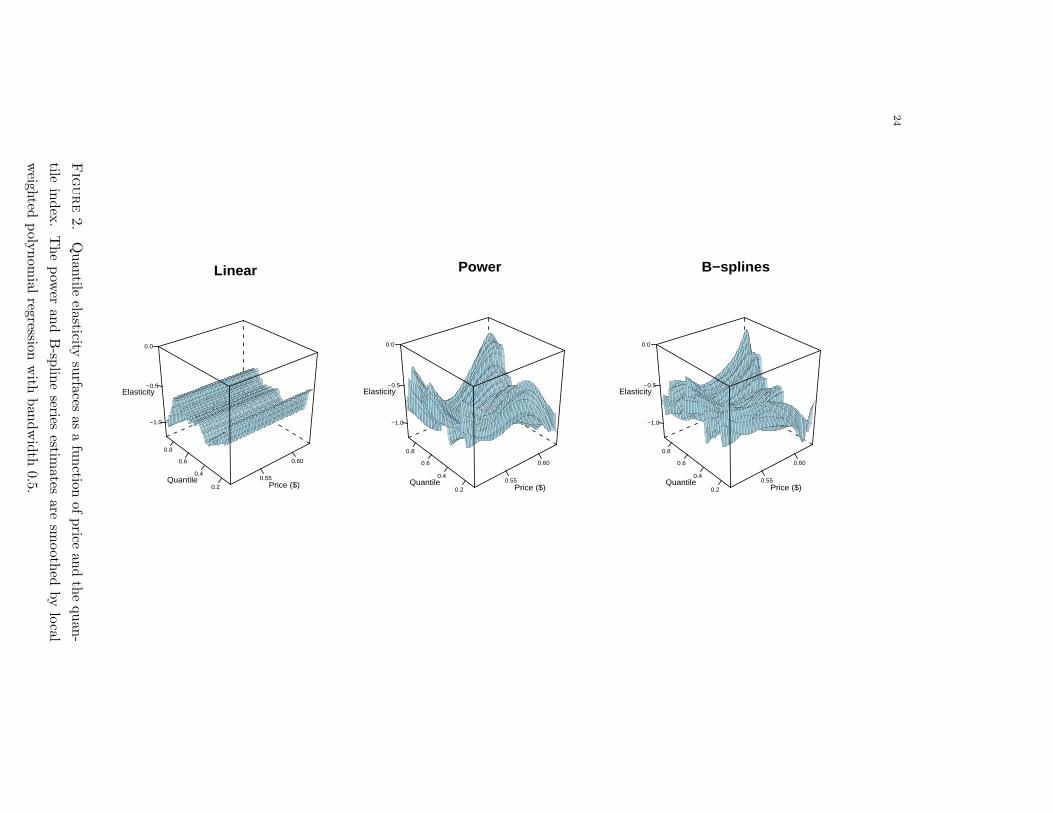
Fig. 2 shows series estimates of the quantile elasticity surface as a function of price and

the quantile index, that is:

(u, exp(w)) 7→ θ(u,w) = ∂wg(w, u).

The estimates from the linear approximation show that the elasticity decreases with the

quantile index in the middle of the distribution, but this pattern is reversed at the tails.

The power and B-spline estimates show substantial heterogeneity of the elasticity across

prices, with individuals at the high quantiles being more sensitive to high prices.3

Fig. 3 shows 90% uniform confidence bands for the average quantile elasticity function

u 7→ θ(u) =

∫∂w g(w, u)dµ(w).

The rows of the figure correspond to the three series approximations and the columns

correspond to the inference methods. We construct the bands using the pivotal, Gaussian

and weighted bootstrap methods. For the pivotal and Gaussian methods the distribution

of the maximal t-statistic is obtained by 1,000 simulations. The weighted bootstrap uses

standard exponential weights and 199 repetitions. The confidence bands show that the

2The median values of the ordinal covariates are $40K for income, 46 for age, and 2 for the number of

drivers. The modal values for the rest of the covariates are 0 for the top-coding of age, 2 for household size,

1 for urban dwellers, 0 for young-single, 0 for the dummy of more than 4 drivers, 4 (Prairie) for province,

and 11 (November) for month.3These estimates are smoothed by local weighted polynomial regression across the price dimension ([16]),

because the unsmoothed elasticity estimates display very erratic behavior.

23

Linear

0.5

0.6

0.7

0.2

0.4

0.6

0.8

200

400

600

800

1000

Price ($)Quantile

Liters

Rearranged

0.5

0.6

0.7

0.2

0.4

0.6

0.8

200

400

600

800

1000

Price ($)Quantile

Liters

Power

0.5

0.6

0.7

0.2

0.4

0.6

0.8

200

400

600

800

1000

Price ($)Quantile

Liters

Rearranged

0.5

0.6

0.7

0.2

0.4

0.6

0.8

200

400

600

800

1000

Price ($)Quantile

Liters

B−splines

0.5

0.6

0.7

0.2

0.4

0.6

0.8

200

400

600

800

1000

Price ($)Quantile

Liters

Rearranged

0.5

0.6

0.7

0.2

0.4

0.6

0.8

200

400

600

800

1000

Price ($)Quantile

Liters

Figure 1. Quantile demand surfaces for gasoline as a function of price and

the quantile index. The left panels display linear, power and B-spline series

estimates and the right panels shows the corresponding estimates mono-

tonized by rearrangement over both dimensions.

24

Linear

0.55

0.60

0.2

0.4

0.6

0.8

−1.0

−0.5

0.0

Price ($)Quantile

Elasticity

Power

0.55

0.60

0.2

0.4

0.6

0.8

−1.0

−0.5

0.0

Price ($)Quantile

Elasticity

B−splines

0.55

0.60

0.2

0.4

0.6

0.8

−1.0

−0.5

0.0

Price ($)Quantile

Elasticity

Figure2.

Quan

tileelasticity

surfaces

asafunction

ofprice

andthequan

-

tileindex.Thepow

eran

dB-sp

lineseries

estimates

aresm

ooth

edbylocal

weigh

tedpoly

nom

ialregression

with

ban

dwidth

0.5.

25

evidence of heterogeneity in the elasticities across quantiles is not statistically significant,

because we can trace a horizontal line within the bands. They show, however, that there is

significant evidence of negative price sensitivity at most quantiles as the bands are bounded

away from zero for most quantiles.

5.2. Numerical Example. To evaluate the performance of our estimation and inference

methods in finite samples, we conduct a Monte Carlo experiment designed to mimic the

previous empirical example. We consider the following design for the data generating pro-

cess:

Y = g(W ) + V ′β + σΦ−1(U), (5.22)

where g(w) = α0 + α1w + α2 sin(2πw) + α3 cos(2πw) + α4 sin(4πw) + α5 cos(4πw), V is

the same covariate vector as in the empirical example, U ∼ U(0, 1), and Φ−1 denotes the

inverse of the CDF of the standard normal distribution. The parameters of g(w) and β

are calibrated by applying least squares to the data set in the empirical example and σ is

calibrated to the least squares residual standard deviation. We consider linear, power and

B-spline series methods to approximate g(w), with the same number of series terms and

other tuning parameters as in the empirical example

Figures 4 and 5 examine the quality of the series approximations in population. They

compare the true quantile function

(u, exp(w)) 7→ θ(u,w) = g(w) + v′β + σΦ−1(u),

and the quantile elasticity function

(u, exp(w)) 7→ θ(u,w) = ∂wg(w),

to the estimands of the series approximations. In the quantile demand function the value of

v is fixed at the sample median values of the ordinal variables and at one for the dummies

corresponding to the sample modal values of the rest of the variables. The estimands are

obtained numerically from a mega-sample (a proxy for infinite population) of 100 × 5, 001

observations with the values of (W,V ) as in the data set (repeated 100 times) and with

Y generated from the DGP (5.22). Although the derivative function does not depend on

u in our design, we do not impose this restriction on the estimands. Both figures show

that the power and B-spline estimands are close to the true target functions, whereas the

more parsimonious linear approximation misses important curvature features of the target

functions, especially in the elasticity function.

26

0.2 0.4 0.6 0.8

−2.

0−

1.5

−1.

0−

0.5

0.0

quantile

Ela

stic

ity

Pivotal

0.2 0.4 0.6 0.8

−2.

0−

1.5

−1.

0−

0.5

0.0

quantile

Ela

stic

ity

Gaussian

0.2 0.4 0.6 0.8

−2.

0−

1.5

−1.

0−

0.5

0.0

quantile

Ela

stic

ity

Weighted Bootstrap

Line

ar

0.2 0.4 0.6 0.8

−2.

0−

1.5

−1.

0−

0.5

0.0

quantile

Ela

stic

ity

Pivotal

0.2 0.4 0.6 0.8

−2.

0−

1.5

−1.

0−

0.5

0.0

quantile

Ela

stic

ity

Gaussian

0.2 0.4 0.6 0.8

−2.

0−

1.5

−1.

0−

0.5

0.0

quantile

Ela

stic

ity

Weighted Bootstrap

Pow

er

0.2 0.4 0.6 0.8

−2.

0−

1.5

−1.

0−

0.5

0.0

quantile

Ela

stic

ity

Pivotal

0.2 0.4 0.6 0.8

−2.

0−

1.5

−1.

0−

0.5

0.0

quantile

Ela

stic

ity

Gaussian

0.2 0.4 0.6 0.8

−2.

0−

1.5

−1.

0−

0.5

0.0

quantile

Ela

stic

ity

Weighted Bootstrap

B−s

plin

es

Figure 3. 90% Confidence bands for the average quantile elasticity func-

tion. Pivotal and Gaussian bands are obtained by 1,000 simulations.

Weighted bootstrap bands are based on 199 bootstrap repetitions with stan-

dard exponential weights.

27

True

0.5

0.6

0.7

0.2

0.4

0.6

0.8

200

400

600

800

1000

Price ($)Quantile

Liters

Linear

0.5

0.6

0.7

0.2

0.4

0.6

0.8

200

400

600

800

1000

Price ($)Quantile

Liters

Power

0.5

0.6

0.7

0.2

0.4

0.6

0.8

200

400

600

800

1000

Price ($)Quantile

Liters

B−spline

0.5

0.6

0.7

0.2

0.4

0.6

0.8

200

400

600

800

1000

Price ($)Quantile

Liters

Figure 4. Estimands of the quantile demand surface. Estimands for the

linear, power and B-spline series estimators are obtained numerically using

500,100 simulations.

28

True

0.50

0.55

0.60

0.65

0.2

0.4

0.6

0.8

−1.0

−0.5

0.0

Price ($)Quantile

Elasticity

Linear

0.50

0.55

0.60

0.65

0.2

0.4

0.6

0.8

−1.0

−0.5

0.0

Price ($)Quantile

Elasticity

Power

0.50

0.55

0.60

0.65

0.2

0.4

0.6

0.8

−1.0

−0.5

0.0

Price ($)Quantile

Elasticity

B−spline

0.50

0.55

0.60

0.65

0.2

0.4

0.6

0.8

−1.0

−0.5

0.0

Price ($)Quantile

Elasticity

Figure 5. Estimands of the quantile elasticity surface. Estimands for the

linear, power and B-spline series estimators are obtained numerically using

500,100 simulations.

29

To analyze the properties of the inference methods in finite samples, we draw 500 samples

from the DGP in equation (5.22) with 3 sample sizes, n: 5, 001, 1, 000, and 500 observations.

For n = 5, 001 we fixW to the values in the data set, whereas for the smaller sample sizes we

draw W with replacement from the values in the data set and keep it fixed across samples.

To speed up computation, we drop the vector V by fixing it at the sample median values

of the ordinal components and at one for the dummies corresponding to the sample modal

values for all the individuals. We focus on the average quantile elasticity function

u 7→ θ(u) =

∫∂wg(w)dµ(w),

over the region I = [0.1, 0.9]. We estimate this function using linear, power and B-spline

quantile regression with the same number of terms and other tuning parameters as in the

empirical example. Although θ(u) does not change with u in our design, again we do not

impose this restriction on the estimators. For inference, we compare the performance of

90% confidence bands for the entire elasticity function. These bands are constructed using

the pivotal, Gaussian and weighted bootstrap methods, all implemented in the same fashion

as in the empirical example. The interval I is approximated by a finite grid of 91 quantiles

I = 0.10, 0.11, ..., 0.90.Table 1 reports estimation and inference results averaged across 200 simulations. The

true value of the elasticity function is θ(u) = −0.74 for all u ∈ I. Bias and RMSE are

the absolute bias and root mean squared error integrated over I. SE/SD reports the ratios

of empirical average standard errors to empirical standard deviations. SE/SD uses the

analytical standard errors from expression (4.11). The bandwidth for Jm(u) is chosen using

the Hall-Sheather option of the quantreg R package ([19]). Length gives the empirical

average of the length of the confidence band. SE/SD and length are integrated over the

grid of quantiles I. Cover reports empirical coverage of the confidence bands with nominal

level of 90%. Stat is the empirical average of the 90% quantile of the maximal t-statistic used

to construct the bands. Table 1 shows that the linear estimator has higher absolute bias

than the more flexible power and B-spline estimators, but displays lower rmse, especially

for small sample sizes. The analytical standard errors provide good approximations to the

standard deviations of the estimators. The confidence bands have empirical coverage close

to the nominal level of 90% for all the estimators and sample sizes considered; and weighted

bootstrap bands tend to have larger average length than the pivotal and Gaussian bands.

30

All in all, these results strongly confirm the practical value of the theoretical results and

methods developed in the paper. They also support the empirical example by verifying that

our estimation and inference methods work quite nicely in a very similar setting.

Table 1. Finite Sample Properties of Estimation and Inference Methods

for Average Quantile Elasticity Function

Pivotal Gaussian Weighted Bootstrap

n = 5, 001

Bias RMSE SE/SD Cover Length Stat Cover Length Stat Cover Length Stat

Linear 0.05 0.14 1.04 90 0.77 2.64 90 0.76 2.64 87 0.82 2.87

Power 0.00 0.15 1.03 91 0.85 2.65 91 0.85 2.65 88 0.91 2.83

B-spline 0.01 0.15 1.02 90 0.86 2.64 88 0.86 2.64 90 0.93 2.84

n = 1, 000

Linear 0.03 0.29 1.09 92 1.78 2.64 93 1.78 2.64 90 1.96 2.99

Power 0.03 0.33 1.07 92 2.01 2.66 91 2.00 2.65 95 2.17 2.95

B-spline 0.02 0.35 1.05 90 2.08 2.65 90 2.07 2.65 96 2.21 2.95

n = 500

Linear 0.04 0.45 1.01 88 2.60 2.64 88 2.60 2.64 90 2.84 3.05

Power 0.02 0.52 1.04 90 3.12 2.65 90 3.13 2.66 95 3.29 3.01

B-spline 0.02 0.52 1.04 90 3.25 2.65 90 3.25 2.65 96 3.35 3.00

Notes: 200 repetitions. Simulation standard error for coverage probability is 2%.

31

Appendix A. Implementation Algorithms

Throughout this section we assume that we have a random sample (Yi, Zi) : 1 ≤ i ≤ n.We are interested in approximating the distribution of the process

√n(β(·) − β(·)) or of

the statistics associated with functionals of it. Recall that for each quantile u ∈ U ⊂ (0, 1),

we estimate β(u) by quantile regression β(u) = argminβ∈Rm En[ρu(Yi − Z ′iβ)], the Gram

matrix Σm by Σm = En[ZiZ′i], and the Jacobian matrix Jm(u) by Powell [32] estimator

Jm(u) = En[1|Yi−Z ′iβ(u)| ≤ hn·ZiZ

′i]/2hn, where we recommend choosing the bandwidth

hn as in the quantreg R package with the Hall-Sheather option ([19]).

We begin describing the algorithms to implement the methods to approximate the dis-

tribution of the process√n(β(·)− β(·)) indexed by U .

Algorithm 1 (Pivotal method). (1) For b = 1, . . . , B, draw U b1 , . . . , U

bn i.i.d. from U ∼

Uniform(0, 1) and compute Ubn(u) = n−1/2

∑ni=1 Zi(u − 1U b

i ≤ u), u ∈ U . (2) Ap-

proximate the distribution of √n(β(u) − β(u)) : u ∈ U by the empirical distribution of

J−1m (u)Ub

n(u) : u ∈ U , 1 ≤ b ≤ B.

Algorithm 2 (Gaussian method). (1) For b = 1, . . . , B, generate a m-dimensional standard

Brownian bridge on U , Bbm(·). Define Gb

n(u) = Σ−1/2m Bb

m(u) for u ∈ U . (2) Approximate the

distribution of √n(β(u) − β(u)) : u ∈ U by the empirical distribution of J−1m (u)Gb

n(u) :

u ∈ U , 1 ≤ b ≤ B.

Algorithm 3 (Weighted bootstrap method). (1) For b = 1, . . . , B, draw hb1, . . . , hbn i.i.d.

from the standard exponential distribution and compute the weighted quantile regression

process βb(u) = argminβ∈Rm

∑ni=1 h

bi ·ρu(Yi−Z ′

iβ), u ∈ U . (2) Approximate the distribution

of √n(β(u)−β(u)) : u ∈ U by the empirical distribution of √n(βb(u)−β(u)) : u ∈ U , 1 ≤b ≤ B.

Algorithm 4 (Gradient bootstrap method). (1) For b = 1, . . . , B, draw U b1 , . . . , U

bn i.i.d.

from U ∼ Uniform(0, 1) and compute Ubn(u) = n−1/2

∑ni=1 Zi(u− 1U b

i ≤ u), u ∈ U . (2)For b = 1, . . . , B, estimate the quantile regression process βb(u) = argminβ∈Rm

∑ni=1 ρu(Yi−

Z ′iβ) + ρu(Yn+1 − Xb

n+1(u)′β), u ∈ U , where Xb

n+1(u) = −√n U

bn(u)/u, and Yn+1 =

nmax1≤i≤n |Yi| to ensure Yn+1 > Xbn+1(u)

′βb(u), for all u ∈ U . (3) Approximate the

distribution of √n(β(u)−β(u)) : u ∈ U by the empirical distribution of √n(βb(u)−β(u)) :u ∈ U , 1 ≤ b ≤ B.

The previous algorithms provide approximations to the distribution of√n(β(u)− β(u))

that are uniformly valid in u ∈ U . We can use these approximations directly to make

32

inference on linear functionals of QY |X(·|X) including the conditional quantile functions,

provided the approximation error is small as stated in Theorems 9 and 11. Each linear

functional is represented by θ(u,w) = ℓ(w)′β(u) + rn(u,w) : (u,w) ∈ I, where ℓ(w)′β(u)is the series approximation, ℓ(w) ∈ R

m is a loading vector, rn(u,w) is the remainder term,

and I is the set of pairs of quantile indices and covariates values of interest, see Section

4 for details and examples. Next we provide algorithms to conduct pointwise or uniform

inference over linear functionals.

Let B be a pre-specified number of bootstrap or simulation repetitions.

Algorithm 5 (Pointwise Inference for Linear Functionals). (1) Compute the variance esti-

mate σ2n(u,w) = u(1−u)ℓ(w)′J−1m (u)ΣmJ

−1m (u)ℓ(w)/n. (2) Using any of the Algorithms 1-4,

compute vectors V1(u), . . . , VB(u) whose empirical distribution approximates the distribution

of√n(β(u) − β(u)). (3) For b = 1, . . . , B, compute the t-statistic t∗bn (u,w) =

∣∣∣ ℓ(w)′Vb(u)√nσn(u,w)

∣∣∣.(4) Form a (1− α)-confidence interval for θ(u,w) as ℓ(w)′β(u)± kn(1− α)σn(u,w), where

kn(1− α) is the 1− α sample quantile of t∗bn (u,w) : 1 ≤ b ≤ B.

Algorithm 6 (Uniform Inference for Linear Functionals). (1) Compute the variance es-

timates σ2n(u,w) = u(1 − u)ℓ(w)′J−1m (u)ΣmJ

−1m (u)ℓ(w)/n for (u,w) ∈ I. (2) Using any

of the Algorithms 1-4, compute the processes V1(·), . . . , VB(·) whose empirical distribution

approximates the distribution of √n(β(u)− β(u)) : u ∈ U. (3) For b = 1, . . . , B, compute

the maximal t-statistic ‖t∗bn ‖I = sup(u,w)∈I

∣∣∣ ℓ(w)′Vb(u)√nσn(u,w)

∣∣∣. (4) Form a (1− α)-confidence band

for θ(u,w) : (u,w) ∈ I as ℓ(w)′β(u) ± kn(1− α)σn(u,w) : (u,w) ∈ I, where kn(1 − α)

is the 1− α sample quantile of ‖t∗bn ‖I : 1 ≤ b ≤ B.

Appendix B. A result on identification of QR series approximation in

population and its relation to the best L2-approximation

In this section we provide results on identification and approximation properties for the

QR series approximation. In what follows, we denote z = Z(x) ∈ Z for some x ∈ X , and

for a function h : X → R we define

Qu(h) = E[ρu(Y − h(X))],

so that β(u) ∈ argminβ∈Rm Qu(Z′β). Also let f := infu∈U ,X∈X fY |X(QY |X(u|X)|X), where

f > 0 by condition S.2.

33

Consider the best L2-approximation to the conditional quantile function gu(·) = QY |X(u|·)by a linear combination of the chosen basis, namely

β∗(u) ∈ arg min

β∈RmE[|Z ′β − gu(X)|2

]. (B.23)

We consider the following approximation rates associated with β∗(u):

c2u,2 = E[|Z ′β

∗(u)− gu(X)|2

]and cu,∞ = sup

x∈X ,z=Z(x)|z′β∗

(u)− gu(x)|.

Lemma 1. Assume that conditions S.2-S.4, ζmcu,2 = o(1) and cu,∞ = o(1) hold. Then, as

n grows, we have the following approximation properties for β(u):

E[|Z ′β(u)− gu(X)|2

]≤ (16 ∨ 3f/f)c2u,2, E

[|Z ′β(u)− Z ′β

∗(u)|2

]≤ (9 ∨ 8f /f)c2u,2 and

supx∈X ,z=Z(x)

|z′β(u)− gu(x)| . cu,∞ + ζm

√(9 ∨ 8f /f)cu,2/

√mineig(Σm).

Proof of Lemma 1. We assume that E[|Z ′β(u)− Z ′β

∗(u)|2

]1/2≥ 3E

[|Z ′β

∗(u)− gu(X)|2

]1/2,

otherwise the statements follow directly. The proof proceeds in 4 steps.

Step 1 (Main argument). For notational convenience let

q = (f3/2/f ′)E[|Z ′β(u)− gu(X)|2

]3/2/E[|Z ′β(u)− gu(X)|3

].

By Steps 2 and 3 below we have respectively

Qu(Z′β(u)) −Qu(gu) ≤ f c2u,2 and (B.24)

Qu(Z′β(u))−Qu(gu) ≥

fE[|Z ′β(u)− gu(X)|2

]

3∧( q3

√fE [|Z ′β(u)− gu(X)|2]

). (B.25)

Thus

fE[|Z′β(u)−gu(X)|2]3 ∧

(q/3)

√fE [|Z ′β(u)− gu(X)|2]

≤ f c2u,2.

As n grows, since√f c2u,2 < q/

√3 by Step 4 below, it follows that E

[|Z ′β(u)− gu(X)|2

]≤

3c2u,2f/f which proves the first statement regarding β(u).

The second statement regarding β(u) follows since√E[|Z ′β(u)− Z ′β∗(u)|2

]≤√E [|Z ′β(u)− gu(X)|2]+

√E[|Z ′β∗(u)− gu(X)|2

]≤√3c2u,2f/f+cu,2.

34

Finally, the third statement follows by the triangle inequality, S.4, and the second state-

ment

supx∈X ,z=Z(x) |z′β(u)− gu(x)| ≤ supx∈X ,z=Z(x) |z′β∗(u)− gu(x)|+ ζm‖β(u)− β

∗(u)‖

≤ cu,∞ + ζm

√E[|Z ′β∗(u)− Z ′β(u)|2

]/mineig(Σm)

≤ cu,∞ + ζm

√(9 ∨ 8f /f)cu,2/

√mineig(Σm).

Step 2 (Upper Bound). For any two scalars w and v we have that

ρu(w − v)− ρu(w) = −v(u− 1w ≤ 0) +∫ v

0(1w ≤ t − 1w ≤ 0)dt. (B.26)

By (B.26) and the law of iterated expectations, for any measurable function h

Qu(h)−Qu(gu) = E[∫ h−gu

0 FY |X(gu + t|X)− FY |X(gu|X)dt]

= E[∫ h−gu

0 tfY |X(gu + tX,t|X)dt]≤ (f /2)E[|h − gu|2]

(B.27)

where tX,t lies between 0 and t for each t ∈ [0, h(x) − gu(x)].

Thus, (B.27) with h(X) = Z ′β∗(u) and Qu(Z

′β(u)) ≤ Qu(Z′β

∗(u)) imply that

Qu(Z′β(u))−Qu(gu) ≤ Qu(Z

′β∗(u))−Qu(gu) ≤ f c2u,2.

Step 3 (Lower Bound). To establish a lower bound note that for a measurable function h

Qu(h)−Qu(gu) = E[∫ h−gu

0 FY |X(gu + t|X)− FY |X(gu|X)dt]

= E[∫ h−gu

0 tfY |X(gu|X) + t2

2 f′Y |X(gu + tX,t|X)dt

]

≥ (f/2)E[|h − gu|2]− 16 f

′E[|h− gu|3].(B.28)

If√fE [|Z ′β(u)− gu(X)|2] ≤ q, then f ′E

[|Z ′β(u)− gu(X)|3

]≤ fE

[|Z ′β(u)− gu(X)|2

]

and (B.28) with the function h(Z) = Z ′β(u) yields

Qu(Z′β(u))−Qu(gu) ≥

fE[|Z ′β(u)− gu(X)|2

]

3.

On the other hand, if√fE [|Z ′β(u)− gu(X)|2] > q, let hu(X) = (1−α)Z ′β(u)+αgu(X)

where α ∈ (0, 1) is picked so that√fE [|hu − gu|2] = q. Then by (B.28) and convexity of

Qu we have

Qu(Z′β(u))−Qu(gu) ≥

√fE [|Z ′β(u)− gu(X)|2]

q· ( Qu(hu)−Qu(gu) ) .

35

Next note that hu(X) − gu(X) = (1− α)(Z ′β(u)− gu(X)), thus

√fE [|hu − gu|2] = q =

f3/2

f ′E[|Z ′β(u) − gu(X)|2]3/2E[|Z ′β(u) − gu(X)|3] =

f3/2

f ′E[|hu − gu|2]3/2E[|hu − gu|3]

.

Using that and applying (B.28) with hu we obtain

Qu(hu)−Qu(gu) ≥ (f/2)E[|hu − gu|2]−1

6f ′E[|hu − gu|3] = q2/3.

Therefore

Qu(Z′β(u)) −Qu(gu) ≥

fE[|Z ′β(u)− gu(X)|2

]

3∧( q3

√fE [|Z ′β(u)− gu(X)|2]

).

Step 4. (f c2u,2 < q2/3 as n grows) Recall that by S.4 ‖Z‖ ≤ ζm and that we can assume

E[|Z ′β(u) − Z ′β

∗(u)|2

]1/2≥ 3E

[|Z ′β

∗(u)− gu(X)|2

]1/2.

Then, using the relation above (in the second inequality)

E[|Z′β(u)−gu(X)|2]3/2

E[|Z′β(u)−gu(X)|3] ≥ E[|Z′β(u)−gu(X)|2]1/2

supx∈X ,z=Z(x) |z′β(u)−gu(x)|

≥ 12

E[|Z′β(u)−Z′β

∗(u)|2

]1/2+E

[|Z′β

∗(u)−gu(X)|2

]1/2

supx∈X ,z=Z(z) |z′β(u)−z′β∗(u)|+supx∈X ,z=Z(x) |z′β∗(u)−gu(x)|

≥ 12

(E[|Z′β(u)−Z′β

∗(u)|2

]1/2

supx∈X ,z=Z(x) |z′β(u)−z′β∗ (u)| ∧E[|Z′β

∗(u)−gu(X)|2

]1/2

supx∈X ,z=Z(x) |z′β∗(u)−gu(x)|

)

≥ 12

(κ‖β(u)−β

∗(u)‖

ζm‖β(u)−β∗(u)‖ ∧ cu,2

cu,∞

)

where κ =√

mineig(Σm).

Finally,√f cu,2 < (f3/2/f ′)(1/2)( κ

ζm∧ cu,2

cu,∞)/√3 ≤ q/

√3 as n grows under the condition

ζmcu,2 = o(1), cu,∞ = o(1), and conditions S.2 and S.3.

Appendix C. Proof of Theorems 1-7

In this section we gather the proofs of the theorems 1-7 stated in the main text. We adopt

the standard notation of the empirical process literature [37]. We begin by assuming that

the sequences m and n satisfy m/n→ 0 as m,n→ ∞. For notational convenience we write

ψi(β, u) = Zi(1Yi ≤ Z ′iβ − u), where Zi = Z(Xi). Also for any sequence r = rn = o(1)

and any fixed 0 < B <∞, we define the set

Rn,m := (u, β) ∈ U × Rm : ‖β − β(u)‖ ≤ Br

36

and the following error terms:

ǫ0(m,n) := supu∈U

‖Gn(ψi(β(u), u))‖,

ǫ1(m,n) := sup(u,β)∈Rn,m

‖Gn(ψi(β, u)) −Gn(ψi(β(u), u))‖,

ǫ2(m,n) := sup(u,β)∈Rn,m

n1/2‖E[ψi(β, u)] − E[ψi(β(u), u)] − Jm(u)(β − β(u))‖.

In what follows, we say that the data are in general position if for any γ ∈ Rm,

P (Yi = Z ′iγ, for at least one i) = 0. Under the bounded density condition S.2, the data

are in the general position. We also assume i.i.d. sampling throughout the appendix,

although this condition is not needed for most of the results.

C.1. Proof of Theorem 1. We start by establishing uniform rates of convergence. The

following technical lemma will be used in the proof of Theorem 1.

Lemma 2 (Rates in Euclidian Norm for Perturbed QR Process). Suppose that β(u) is a

minimizer of

En[ρu(Yi − Z ′iβ)] +An(u)

′β

for each u ∈ U , and that the perturbation term obeys supu∈U ‖An(u)‖ .P r = o(1). The

unperturbed case corresponds to An(·) = 0. If infu∈U mineig [Jm(u)] > J > 0 and the

conditions

R1. ǫ0(m,n) .P√nr,

R2. ǫ1(m,n) .P√nr,

R3. ǫ2(m,n) .P√nr,

hold, where the constants in the bounds above can be taken to be independent of the constant

B in the definition of Rm,n, then for any ε > 0, there is a sufficiently large B such that

with probability at least 1− ε, (u, β(u)) ∈ Rm,n uniformly over u ∈ U , that is,

supu∈U

∥∥∥β(u)− β(u)∥∥∥ .P r. (C.29)

Proof of Lemma 2. Due to the convexity of the objective function, it suffices to show that

for any ε > 0, there exists B <∞ such that

P

(infu∈U

inf‖η‖=1

η′ [En [ψi (β, u)] +An(u)] |β=β(u)+Brη > 0

)≥ 1− ε. (C.30)

37

Indeed, the quantity En [ψi (β, u)] + An(u) is a subgradient of the objective function at β.

Observe that uniformly in u ∈ U ,√nη′En [ψi (β(u) +Brη, u)] ≥ Gn(η

′ψi(β(u), u)) + η′Jm(u)ηB√nr − ǫ1(m,n)− ǫ2(m,n),

since E [ψi(β(u), u)] = 0 by definition of β(u) (see argument in the proof of Lemma 3).

Invoking R2 and R3,

ǫ1(m,n) + ǫ2(m,n) .P

√nr,

and by R1, uniformly in η ∈ Sm−1 we have

|Gn(η′ψi(β(u), u))| ≤ sup

u∈U‖Gn(ψi(β(u), u))‖ = ǫ0(m,n) .P

√nr.

Then the event of interest in (C.30) is implied by the eventη′Jm(u)ηB

√nr − ǫ0(m,n)− ǫ1(m,n)− ǫ2(m,n)−

√n sup

u∈U‖An(u)‖ > 0

,

whose probability can be made arbitrarily close to 1, for large n, by setting B sufficiently

large since supu∈U ‖An(u)‖ .P r, and η′Jm(u)η ≥ J > 0 by the condition on the eigenvalues

of Jm(u).

Proof of Theorem 1. Let φn = supα∈Sm−1 E[(Z ′iα)

2] ∨ En[(Z′iα)

2]. Under ζ2m log n = o(n)

and S.3, φn .P 1 by Corollary 2 in Appendix G.

Next recall that Rm,n = (u, β) ∈ U × Rm : ‖β − β(u)‖ ≤ Br for some fixed B large

enough.

Under S.1-S.5, ǫ0(m,n) .P√mφn log n by Lemma 23, and ǫ1(m,n) .P

√mφn log n

by Lemma 22, where none of these bounds depend on B. Under S.1-S.5, ǫ2(m,n) .√nζmB

2r2 +√nm−κBr .

√nr by Lemma 24 provided ζmB

2r = o(1) and m−κB = o(1).

Finally, since ζ2mm log n = o(n) by the growth condition of the theorem, we can take

r =√

(m log n)/n in Lemma 2 with An(u) = 0 and the result follows.

C.2. Proof of Theorems 2, 3, 4, 5 and 6. In order to establish our uniform linear

approximations for the perturbed QR process, it is convenient to define the following ap-

proximation error:

ǫ3(m,n) := supu∈U

n1/2‖ En[ψi(β(u), u)] +An(u)‖.

Lemma 3 (Uniform Linear Approximation). Suppose that β(u) is a minimizer of

En[ρu(Yi − Ziβ)] +An(u)′β

38

for each u ∈ U , the data are in general position, and the conditions of Lemma 2 hold. The

unperturbed case corresponds to An(·) = 0. Then

√nJm(u)

(β(u)− β(u)

)=

−1√n

n∑

i=1

ψi(β(u), u) −An(u) + rn(u),

supu∈U ‖rn(u)‖ .P ǫ1(m,n) + ǫ2(m,n) + ǫ3(m,n).

(C.31)

Proof of Lemma 3. First note that E [ψi(β(u), u)] = 0 by definition of β(u). Indeed, despite

the possible approximation error, β(u) minimizes E[ρu(Y−Z ′β)] which yields E [ψi(β(u), u)] =

0 by the first order conditions.

Therefore equation (C.31) can be recast as

rn(u) = n1/2Jm(u)(β(u)− β(u)) +Gn (ψi(β(u), u)) +An(u).

Next note that if (u, β(u)) ∈ Rn,m uniformly in u ∈ U by the triangle inequality, uniformly

in u ∈ U

‖rn(u)‖ ≤∥∥∥Gn(ψi(β(u), u)) −Gn(ψi(β(u), u))

∥∥∥ +

+ n1/2∥∥∥E[ψi(β(u), u)

]− E [ψi(β(u), u)] − Jm(u)

(β(u)− β(u)

)∥∥∥+

+ n1/2∥∥∥En

[ψi(β(u), u)

]+An(u)

∥∥∥

≤ ǫ1(m,n) + ǫ2(m,n) + ǫ3(m,m).

The result follows by Lemma 2 which bounds from below the probability of (u, β(u)) ∈ Rn,m

uniformly in u ∈ U .

Proof of Theorem 2. We first control the approximation errors ǫ0, ǫ1, ǫ2, and ǫ3. Lemma

23 implies that ǫ0(m,n) .P√mφn log n. Lemma 24 implies that

ǫ1(m,n) .P

√mζmr log n+

mζm log n√n

and ǫ2(m,n) .P

√nζmr

2 +√nm−κr.

Next note that under the bounded density condition in S.2, the data are in general

position. Therefore, by Lemma 26 with probability 1 we have

ǫ3(m,n) ≤mζm√n.

Thus, the assumptions required by Lemma 3 follow under m3ζ2m log3 n = o(n), the uni-

form rate r =√

(m log n)/n, and the condition on κ.

39

Thus by Lemma 3 with An(·) = 0

√nJm(u)

(β(u)− β(u)

)=

−1√n

n∑

i=1

ψi(β(u), u) + rn(u), where

supu∈U

‖rn(u)‖ .P

√mζmr log n+

mζm log n√n

+m−κ√m log n+

mζm√n.

Next, let

ru :=1√n

n∑

i=1

Zi(1Yi ≤ Z ′iβ(u) +R(Xi, u) − 1Yi ≤ Z ′

iβ(u)).

By Lemma 25 supu∈U ‖ru‖ .P

√m1−κ log n + mζm logn√

n. The result follows since Un(u) =d

1√n

∑ni=1 Zi(u− 1Yi ≤ Z ′

iβ(u) +R(Xi, u)).

Proof of Theorem 3. Note that

supu∈U

‖rn(u)‖ ≤ supα∈Sm−1,u∈U

|α′(J−1m (u)− J−1

m (u))α| supu∈U

‖U∗n(u)‖.

To bound the second term, by Lemma 23

supu∈U

‖U∗n(u)‖ .P

√m log n (C.32)

since φn .P 1 by Corollary 2 in Appendix G under ζ2m log n = o(n).

Next since Jm(u) has eigenvalues bounded away from zero by S.2 and S.3, J−1m (u) also

has eigenvalues bounded above by a constant. Moreover, by Lemma 4

supα∈Sm−1,u∈U

|α′(Jm(u)− Jm(u))α| .P ǫ5(m,n) + ǫ6(m,n)

.P

√ζ2mm logn

nhn+ mζ2m logn

nhn+m−κ +

√m logn

n ζm + hn,

where the second inequality follows by Lemma 28 with r =√

(m log n)/n. Under the growth

conditions stated in the Theorem,

supα∈Sm−1,u∈U

|α′(Jm(u)− Jm(u))α| . oP

(1/

√m log3 n

).

Thus, with probability approaching one, J−1m (u) has eigenvalues bounded above by a con-

stant uniformly in u ∈ U .

40

Moreover, by the matrix identity A−1 −B−1 = B−1(B −A)A−1

|α′(J−1m (u)− J−1

m (u))α| = |α′J−1m (u)(Jm(u)− Jm(u))J−1

m (u)α|≤ ‖α′J−1

m (u)‖ supα∈Sm−1

|α′(Jm(u)− Jm(u))α| ‖J−1m (u)α‖

. oP

(1/√m log3 n

),

(C.33)

which holds uniformly over α ∈ Sm−1 and u ∈ U .Finally, the stated bound on supu∈U ‖rn(u)‖ follows by combining the relations (C.32)

and (C.33).

Proof of Theorem 4. The first part of the proof is similar to the proof of Theorem 2 but

applying Lemma 3 twice, one to the unperturbed problem and one to the perturbed problem

with An(u) = −U∗n(u)/

√n, for every u ∈ U . Consider the set E of realizations of the data

Dn such that sup‖α‖=1 En[(α′Zi)

2] . 1. By Corollary 2 in Appendix G and assumptions S.3

and S.4, P (E) = 1− o(1) under our growth conditions. Thus, by Lemma 23

supu∈U

‖An(u)‖ .P r =

√m log n

n

where we used that φn .P 1 by Corollary 2 in Appendix G under ζ2m log n = o(n) and S.3.

Then,

√nJm(u)

(β∗(u)− β(u)

)=

√nJm(u)

(β∗(u)− β(u)

)−√

nJm(u)(β(u)− β(u)

)

= U∗n(u) + rpertn (u)− runpertn (u), where

supu∈U

‖rpertn (u)− runpertn (u)‖ .P

√mζmr log n+

mζm log n√n

+m−κ√m log n+

mζm√n.

Note also that the results continue to hold in P -probability if we replace P by P ∗, since

if a random variable Bn = OP (1) then Bn = OP ∗(1). Indeed, the first relation means that

P (|Bn| > ℓn) = o(1) for any ℓn → ∞, while the second means that P ∗(|Bn| > ℓn) = oP (1)

for any ℓn → ∞. But the second clearly follows from the first from the Markov inequality,

observing that E[P ∗(|Bn| > ℓn)] = P (|Bn| > ℓn) = o(1).

Proof of Theorem 5. The existence of the Gaussian process with the specified covariance

structure is trivial. To establish the additional coupling, note that under S.1-S.4 and the

growth conditions, sup‖α‖=1 En[(α′Zi)

2] .P 1 by Corollary 2 in Appendix G. Conditioning

on any realization of Z1, ..., Zn such that sup‖α‖=1 En[(α′Zi)

2] . 1, the existence of the

Gaussian process with the specified covariance structure that also satisfies the coupling

41

condition follows from Lemma 8. Under the conditions of the theorem supu∈U ‖Un(u) −Gn(u)‖ = oP (1/ log n). Therefore, the second statement follows since

supu∈U

‖√n(β(u)− β(u)) − J−1m (u)Gn(u)‖

≤ supu∈U

‖J−1m (u)Un(u)− J−1

m (u)Gn(u)‖ + oP (1/ log n)

≤ supu∈U

‖J−1m (u)‖ sup

u∈U‖Un(u)−Gn(u)‖+ oP (1/ log n) = oP (1/ log n),

where we invoke Theorem 2 under the growth conditions, and that the eigenvalues of Jm(u)

are bounded away from zero uniformly in n by S.2 and S.3.

The last statement proceeds similarly to the proof of Theorem 3.

Proof of Theorem 6. Note that βb(u) solves the quantile regression problem for the rescaled

data (hiYi, hiZi) : 1 ≤ i ≤ n. The weight hi is independent of (Yi, Zi), E[hi] = 1,

E[h2i ] = 1, and max1≤i≤n hi .P log n. That allows us to extend all results from β(u) to βb(u)

replacing ζm by ζbm = ζm log n to account for the larger envelope, and ψbi (β, u) = hiψi(β, u).

The first part of the proof is similar to the proof of Theorem 2 but applying Lemma 3

twice, one to the original problem and one to the problem weighted by hi. Then√n(βb(u)− β(u)

)=

√n(βb(u)− β(u)

)+

√n(β(u) − β(u)

)

=J−1m (u)√n

n∑

i=1

hiZi(u− 1Yi ≤ Z ′iβ(u)) + rbn(u)−

−J−1m (u)√n

n∑

i=1

Zi(u− 1Yi ≤ Z ′iβ(u)) − rn(u)

where supu∈U ‖rn(u)− rbn(u)‖ .P

√mζmr log

2 n+ mζm log2 n√n

+m−κ√m log n+ mζm logn√

n.

Next, let

ru :=1√n

n∑

i=1

(hi − 1)Zi(1Yi ≤ Z ′iβ(u) +R(Xi, u) − 1Yi ≤ Z ′

iβ(u)).

By Lemma 25, supu∈U ‖ru‖ .P

√m1−κ log n + ζmm log2 n√

n. The result follows since 1Ui ≤

u = 1Yi ≤ Z ′iβ(u) +R(Xi, u).

Note also that the results continue to hold in P -probability if we replace P by P ∗, since

if a random variable Bn = OP (1) then Bn = OP ∗(1). Indeed, the first relation means that

P (|Bn| > ℓn) = o(1) for any ℓn → ∞, while the second means that P ∗(|Bn| > ℓn) = oP (1)

42

for any ℓn → ∞. But the second clearly follows from the first from the Markov inequality,

observing that E[P ∗(|Bn| > ℓn)] = P (|Bn| > ℓn) = o(1).

The second part of the theorem follows by applying Lemma 8 with vi = hi − 1, where

hi ∼ exp(1) so that E[v2i ] = 1, E[|vi|3] . 1 and max1≤i≤n |vi| .P log n. Lemma 8 implies

that there is a Gaussian process Gn(·) with covariance structure En[ZiZ′i](u∧u′−uu′) such

that

supu∈U

∥∥∥∥∥1√n

n∑

i=1

(hi − 1)Zi(u− 1Ui ≤ u)−Gn(u)

∥∥∥∥∥ .P o(1/ log n).

Combining the result above with the first part of the theorem, the second part follows by

the triangle inequality.

C.3. Proof of Theorem 7 on Matrices Estimation. Consider the following quantities

ǫ4(m,n) = supα∈Sm−1

∣∣∣n−1/2Gn

((α′Zi)

2)∣∣∣ ,

ǫ5(m,n) =n−1/2

2hnsup

α∈Sm−1,(u,β)∈Rm,n

∣∣ Gn

(1|Yi − Z ′

iβ| ≤ hn(α′Zi)2) ∣∣ ,

ǫ6(m,n) = supα∈Sm−1,

(u,β)∈Rm,n

∣∣∣∣1

2hnE[1|Yi − Z ′

iβ| ≤ hn(α′Zi)2]− α′Jm(u)α

∣∣∣∣ ,

where hn is a bandwidth parameter such that hn → 0.

Lemma 4 (Estimation of Variance Matrices and Jacobians). Under the definitions of ǫ4, ǫ5,

and ǫ6 we have

supα∈Sm−1

∣∣∣ α′(Σm −Σm)α∣∣∣ ≤ ǫ4(m,n) sup

α∈Sm−1,u∈U

∣∣∣ α′(Jm(u)− Jm(u))α∣∣∣ ≤ ǫ5(m,n)+ǫ6(m,n).

Proof. The first relation follows by the definition of ǫ4(m,n) and the second by the triangle

inequality and definition of ǫ5(m,n) and ǫ6(m,n).

Proof of Theorem 7. This follows immediately from Lemma 4, Lemma 27, and Lemma 28.

43

Appendix D. Proofs of Theorems 8 and 9

Proof of Theorem 8. By Theorem 2 and P1

|θ(u,w) − θ(u,w)| ≤ |ℓ(u)′(β(u)− β(u))|+ |rn(u,w)|≤ |ℓ(w)′J−1

m (u)Un(u)|√n

+ oP

(‖ℓ(w)‖√n logn

)+ o(‖ℓ(w)‖/√n)

≤ |ℓ(w)′J−1m (u)Un(u)|√

n+ oP

(ξθ(m,w)√n logn

)+ o(ξθ(m,w)/

√n)

where the last inequality follows by ‖ℓ(w)‖ . ξθ(m,w) assumed in P2. Finally, since

E[|ℓ(w)′J−1m (u)Un(u)|2] . ‖ℓ(w)‖2‖J−1

m (u)‖2 supα∈Sm−1 E[(α′Z)2] . ξ2θ(m,w), the result

follows by applying the Chebyshev inequality to establish that |ℓ(w)J−1m (u)Un(u)| .P

ξθ(m,w).

Proof of Theorem 9. By Assumption P1 and Theorem 2

tn(u,w) = ℓ(w)′(β(u)−β(u))σn(u,w) + rn(u,w)

σn(u,w) =ℓ(w)′J−1

m (u)Un(u)√nσn(u,w)

+ oP

(‖ℓ(w)‖√

nσn(u,w) logn

)+ oP

(‖ℓ(w)‖√nσn(u,w)

).

To show that the last two terms are oP (1), note that under conditions S.2 and S.3, σn(u,w) &P

‖ℓ(w)‖/√n since σn(u,w) = (1 + oP (1))σn(u,w) by Theorem 7.

Finally, for any ǫ > 0, E[(ℓ(w)′J−1m (u)Zi)

2/σ2n(u,w)1|ℓ(w)′J−1m (u)Zi| ≥ ǫ

√nσn(u,w)] →

0 under our growth conditions. Thus, by Lindeberg-Feller central limit theorem and

σn(u,w) = (1 + oP (1))σn(u,w), it follows that

ℓ(w)′J−1m (u)Un(u)√nσn(u,w)

→d N(0, 1)

and the first result follows.

The remaining results for t∗n(u,w) follow similarly under the corresponding conditions.

Appendix E. Proofs of Theorems 10-12

Lemma 5 (Entropy Bound). Let W ⊂ Rd be a bounded set, and ℓ : W → R

m be a mapping

in W, such that for ξθ(m) and ξLθ (m) ≥ 1,

‖ℓ(w)‖ ≤ ξθ(m) and ‖ℓ(w) − ℓ(w)‖ ≤ ξLθ (m)‖w − w‖, for all w, w ∈ W.

Moreover, assume that ‖Jm(u)−Jm(u′)‖ ≤ ξ(m)|u−u′| for u, u′ ∈ U in the operator norm,

ξ(m) ≥ 1, and let µ = supu∈U ‖Jm(u)−1‖ > 0. Let Lm be the class of functions

Lm = fu,w(g) = ℓ(w)′J−1m (u)g : u ∈ U , w ∈ W ∪ f(g) = 1

44

where g ∈ B(0, ζm), and let F denote the envelope of Lm, i.e. F = supf∈Lm|f |. Then, for

any ε < ε0, the uniform entropy of Lm is bounded by

supQN(ε‖F‖Q,2,Lm, L2(Q)) ≤

(ε0 + diam(U ×W)K

ε

)d+1

where K := µξLθ ζm + µ2ξθ(m)ξ(m)ζm.

Proof. The uniform entropy bound is based on the proof of Theorem 2 of Andrews [1]. We

first exclude the function constant equal to 1 and compute the Lipschitz constant associated

with the other functions in Lm as follows

|ℓ(w)′J−1m (u)g − ℓ(w)′J−1

m (u)g| = |(ℓ(w) − ℓ(w))′J−1m (u)g + ℓ(w)′(J−1

m (u)− J−1m (u))g|

= |(ℓ(w) − ℓ(w))′J−1m (u)g|+

+|ℓ(w)′J−1m (u)(Jm(u)− Jm(u))J−1

m (u)g|≤ ξLθ (m)‖w − w‖‖J−1

m (u)g‖++‖ℓ(w)′J−1

m (u)‖ ξ(m)|u− u| ‖J−1m (u)g‖

≤ K(‖w − w‖+ |u− u|)

where K := µξLθ ζm + µ2ξθ(m)ξ(m)ζm.

Consider functions fuj,wj , where (uj , wj)’s are points at the centers of disjoint cubes of

diameter ε‖F‖Q,2/K whose union covers U ×W. Thus, for any (u,w) ∈ U ×W

minuj ,wj

‖fu,w − fuj ,wj‖Q,2 ≤ K minuj ,wj

(‖w − wj‖+ |uj − u|) ≤ ε‖F‖Q,2.

Adding (if necessary) the constant function in to the cover, for any measure Q we obtain

N(ε‖F‖Q,2,Lm, L2(Q)) ≤ 1 + (diam(U ×W)K/ε‖F‖Q,2)d+1.

The result follows by noting that ε < ε0 and that ‖F‖Q,2 ≥ 1 since Lm contains the function

constant equal to 1.

Lemma 6. Let F and G be two classes of functions with envelopes F and G respectively.

Then the entropy of FG = fg : f ∈ F , g ∈ G satisfies

supQN(ε‖FG‖Q,2,FG, L2(Q)) ≤ sup

QN((ε/2)‖F‖Q,2,F , L2(Q)) sup

QN((ε/2)‖G‖Q,2,G, L2(Q)).

Proof. The proof is similar to Theorem 3 of Andrews [1]. For any measure Q we denote

cF = ‖F‖2Q,2 and cG = ‖G‖2Q,2. Note for any measurable set A, QF (A) =∫A F

2(x)dQ(x)/cF

and QG(A) =∫AG

2(x)dQ(x)/cG are also measures. Let

K = supQF

N(ε‖G‖QF ,2,G, L2(QF )) = supQN(ε‖G‖Q,2,G, L2(Q)) and

45

L = supQG

N(ε‖F‖QG,2,F , L2(QG)) = supQN(ε‖G‖Q,2,G, L2(Q)).

Let g1, . . . , gK and f1, . . . , fL denote functions in G and F used to build a cover of G and

F of cubes with diameter ε‖FG‖Q,2. Since F ≥ |f | and G ≥ |g| we have

minℓ≤L,k≤K

‖fg − fℓgk‖Q,2 ≤ minℓ≤L,k≤K

‖f(g − gk)‖Q,2 + ‖gk(f − fℓ)‖Q,2

≤ mink≤K

‖F (g − gk)‖Q,2 +minℓ≤L

‖G(f − fℓ)‖Q,2

= mink≤K

‖(g − gk)‖QF ,2 +minℓ≤L

‖(f − fℓ)‖QG,2

≤ ε‖G‖QF ,2 + ε‖F‖QG,2 = 2ε‖FG‖Q,2.

Therefore, by taking pairwise products of g1, . . . , gK and f1, . . . , fL to create a net we

have

N(ε‖FG‖Q,2,FG, L2(Q)) ≤ N((ε/2)‖F‖Q,2,F , L2(Q)) N((ε/2)‖G‖Q,2,G, L2(Q)).

The result follows by taking the supremum over Q on both sides.

Proof of Theorem 10. By the triangle inequality

sup(u,w)∈I

|θ(u,w) − θ(u,w)| ≤ sup(u,w)∈I

|ℓ(w)′(β(u)− β(u))| + sup(u,w)∈I

|rn(u,w)|

where the second term satisfies sup(u,w)∈I | rn(u,w)/‖ℓ(w)‖ | = o(n−1/2 log−1 n) by condi-

tion U.1.

By Theorem 2, the first term is bounded uniformly over I by

|ℓ(w)′(β(u)− β(u))| .P|ℓ(w)′J−1

m (u)Un(u)|√n

+ oP (ξθ(m, I)/[√n log n]) (E.34)

since ‖ℓ(w)‖ ≤ ξθ(m, I) by U.2 and the remainder term of the linear representation in

Theorem 2 satisfies supu∈U ‖rn(u)‖ = oP (1/ log n).

Given Zi = Z(Xi) consider the classes of functions

Fm = ℓ(w)′J−1m (u)Zi : (u,w) ∈ I, G = (1Ui ≤ u−u) : u ∈ U and Lm = Fm∪f(Zi) = 1.

By Lemma 5 and Lemma 6 the entropy of the class of function LmG = fg : f ∈ Lm, g ∈G satisfies, for K . (ξθ(m, I) ∨ 1)(ξLθ (m, I) ∨ 1)(ζm ∨ 1),

supQ

logN(ε‖F‖2,Q,LmG, L2(Q)) . (d+ 1) log[(1 + diam(I)K)/ε] . log(n/ε)

by our assumptions. Noting that under S.3

sup(u,w)∈I

√u(1− u)ℓ(w)′J−1

m (u)ΣmJ−1m (u)ℓ(w) . ξθ(m, I),

46

Lemma 16 applied to LmG with J(m) =√d log n, M(m,n) . 1 ∨ ξθ(m, I)ζm yields

sup(u,w)∈I

|ℓ(w)′Jm(u)−1Un(u)| .P

√d logn

(1 ∨ ξ2θ(m, I) +

d log(n) (1 ∨ ξ2θ (m, I) ζ2m) logn

n

)1/2

log1/2 n

where the second term in the parenthesis is negligible compared to the first under our

growth conditions. The result follows using this bound into (E.34).

Proof of Theorem 11. Under the conditions of Theorems 2 and 3, supu∈U |maxeig(J−1m (u)−

J−1m (u))| .P o(1/

√m log3/2 n), and σn(u,w) = (1 + oP (1/

√m log3/2 n))σn(u,w) uniformly

in (u,w) ∈ I. Note that σn(u,w) &P ‖ℓ(w)‖/√n. Next define t∗n(u,w) as follows:

For pivotal and gradient bootstrap coupling: t∗n(u,w) =ℓ(w)′J−1

m (u)U∗n(u)/

√n

σn(u,w);

For Gaussian and weighted bootstrap coupling: t∗n(u,w) =ℓ(w)′J−1

m (u)Gn(u)/√n

σn(u,w).

Note that t∗n is independent of the data conditional on the regressor sequence Zn = (Z1, ..., Zn),

unlike t∗n which has some dependence on the data through various estimated quantities.

For the case of pivotal and gradient bootstrap couplings by Theorem 2 and condition U

tn(u,w) =d t∗n(u,w) + oP (1/ log n) in ℓ∞(I).

Moreover, for the case of Gaussian and weighted bootstrap couplings under the conditions

of Theorem 5

tn(u, n) =d t∗n(u,w) + oP (1/ log n) in ℓ∞(I).

Finally, under the growth conditions

t∗n(u,w) = t∗n(u,w) + oP (1/ log n) in ℓ∞(I).

Thus, it follows that uniformly in (u,w) ∈ I

tn(u,w) =d t∗n(u,w) + oP (1/ log n) = tn(u,w) + oP (1/ log n)

and the result follows.

Proof of Theorem 12. Let εn = 1/ log n, and δn such that δn log1/2 n→ 0, and δn/εn → ∞.

47

Step 1. By the proof of Theorem 11 there is an approximation ‖t∗n‖I = sup(u,w)∈I |t∗n(u,w)|to ‖t∗n‖I = sup(u,w)∈I |t∗n(u,w)|, which does not depend on the data conditional on the re-

gressor sequence Zn = (Z1, ..., Zn), such that

P (| ‖t∗n‖I − ‖t∗n‖I | ≤ εn) = 1− o(1).

Now let

kn(1− α) := (1− α)− quantile of ‖t∗n‖I , conditional on Dn,

and let

κn(1− α) := (1− α)− quantile of ‖t∗n‖I , conditional on Dn.

Note that since ‖t∗n‖I is conditionally independent of Y1, . . . , Yn,

κn(1− α) = (1− α)− quantile of ‖t∗n‖I , conditional on Zn.

Then applying Lemma 7 to ‖t∗n‖I and ‖t∗n‖I , we get that for some νn ց 0

P [κn(p) ≥ kn(p − νn)− εn and kn(p) ≥ κn(p− νn)− εn] = 1− o(1).

Step 2. Claim (1) now follows by noting that

P‖tn‖I > kn(1− α) + δn ≤ P‖tn‖I > κn(1− α− νn)− εn + δn+ o(1)

≤ P‖t∗n‖I > κn(1− α− νn)− 2εn + δn+ o(1)

≤ P‖t∗n‖I > kn(1− α− 2νn)− 3εn + δn+ o(1)

≤ P‖t∗n‖I > kn(1− α− 2νn)+ o(1)

= EP [P‖t∗n‖I > kn(1− α− 2νn)|Dn] + o(1)

≤ EP [α+ 2νn] + o(1) = α+ o(1).

Claim (2) follows from the equivalence of the event θ(u,w) ∈ [ι(u,w), ι(u,w)], for all

(u,w) ∈ I and the event ‖tn‖I ≤ cn(1 − α).To prove Claim (3) note that σn(u,w) = (1 + oP (1))σn(u,w) uniformly in (u,w) ∈ I

under the conditions of Theorems 2 and 7. Moreover, cn(1 − α) = kn(1 − α)(1 + oP (1))

because 1/kn(1− α) .P 1 and δn → 0. Combining these relations the result follows.

Claim (4) follows from Claim (1) and from the following lower bound.

By Lemma 7, we get that for some νn ց 0

P [κn(p + νn) + εn ≥ kn(p) and kn(p+ νn) + εn ≥ κn(p)] = 1− o(1).

48

Then

P‖tn‖I ≥ kn(1− α) + δn ≥ P‖tn‖I ≥ κn(1− α+ νn) + εn + δn − o(1)

≥ P‖t∗n‖I ≥ κn(1− α+ νn) + 2εn + δn − o(1)

≥ P‖t∗n‖I ≥ kn(1− α+ 2νn) + 3εn + δn − o(1)

≥ P‖t∗n‖I ≥ kn(1− α+ 2νn) + 2δn − o(1)

≥ E[P‖t∗n‖I ≥ kn(1− α+ 2νn) + 2δn|Dn]− o(1)

= α− 2νn − o(1) = α− o(1),

where we used the anti-concentration property in the last step.

We use this lemma in the proof of Theorem 12.

Lemma 7 (Closeness in Probability Implies Closeness of Conditional Quantiles). Let Xn

and Yn be random variables and Dn be a random vector. Let FXn(x|Dn) and FYn(x|Dn)

denote the conditional distribution functions, and F−1Xn

(p|Dn) and F−1Yn

(p|Dn) denote the

corresponding conditional quantile functions. If |Xn − Yn| = oP (ε), then for some νn ց 0

with probability converging to one

F−1Xn

(p|Dn) ≤ F−1Yn

(p+ νn|Dn) + ε and F−1Yn

(p|Dn) ≤ F−1Xn

(p+ νn|Dn) + ε,∀p ∈ (νn, 1− νn).

Proof. We have that for some νn ց 0, P|Xn − Yn| > ε = o(νn). This implies that

P [P|Xn − Yn| > ε|Dn ≤ νn] → 1, i.e. there is a set Ωn such that P (Ωn) → 1 and

P|Xn − Yn| > ε|Dn ≤ νn for all Dn ∈ Ωn. So, for all Dn ∈ Ωn

FXn(x|Dn) ≥ FYn+ε(x|Dn)− νn and FYn(x|Dn) ≥ FXn+ε(x|Dn)− νn,∀x ∈ R,

which implies the inequality stated in the lemma, by definition of the conditional quantile

function and equivariance of quantiles to location shifts.

Appendix F. A Lemma on Strong Approximation of an Empirical Process of

an Increasing Dimension by a Gaussian Process

Lemma 8. (Approximation of a Sequence of Empirical Processes of Increasing Dimension

by a Sequence of Gaussian Processes) Consider the empirical process Un in [ℓ∞(U)]m, U ⊆(0, 1), conditional on Zi ∈ R

m, i = 1, . . . , n, defined by

Un(u) = Gn (viZiψi(u)) , ψi(u) = u− 1Ui ≤ u,

49

where Ui, i = 1, . . . , n, is an i.i.d. sequence of standard uniform random variables, vi, i =

1, . . . , n, is an i.i.d. sequence of real valued random variables such that E[v2i ] = 1, E[|vi|3] .1, and max1≤i≤n |vi| .P log n. Suppose that Zi, i = 1, . . . , n, are such that

sup‖α‖≤1

En

[(α′Zi)

2]. 1, max

1≤i≤n‖Zi‖ . ζm, and m7ζ6m log22 n = o(n).

There exists a sequence of zero-mean Gaussian processes Gn with a.s. continuous paths,

that has the same covariance functions as Un, conditional on Z1, . . . , Zn, namely,

E[Gn(u)Gn(u′)′] = E[Un(u)Un(u

′)′] = En[ZiZ′i](u ∧ u′ − uu′), for all u and u′ ∈ U ,

and that approximates the empirical process Un, namely,

supu∈U

‖Un(u)−Gn(u)‖ .P o

(1

log n

).

Proof. The proof is based on the use of maximal inequalities and Yurinskii’s coupling.

Throughout the proof all the probability statements are conditional on Z1, . . . , Zn.

We define the sequence of projections πj : U → U , j = 0, 1, 2, . . . ,∞ by πj(u) = 2k−1/2j

if u ∈ ((2k − 2)/2j , 2k/2j), k = 1, . . . , j, and πj(u) = u if u = 0 or 1. In what follows, given

a process G in [ℓ∞(U)]m and its projection G πj, whose paths are step functions with

2j steps, we shall identify the process G πj with a random vector G πj in R2jm, when

convenient. Analogously, given a random vector W in R2jm we identify it with a process

W in [ℓ∞(U)]m, whose paths are step functions with 2j steps.

The following relations proven below:

(1) (Finite-Dimensional Approximation)

r1 = supu∈U

‖Un(u)− Un πj(u)‖ .P o

(1

log n

);

(2) (Coupling with a Normal Vector) there exists Nnj =d N(0, var[Un πj ]) such that,

r2 = ‖Nnj − Un πj‖2 .P o

(1

log n

);

(3) (Embedding a Normal Vector into a Gaussian Process) there exists a Gaussian

process Gn with properties stated in the lemma such that Nnj = Gn πj a.s.;

(4) (Infinite-Dimensional Approximation)

r3 = supu∈U

‖Gn(u)−Gn πj(u)‖ .P o

(1

log n

).

50

The result then follows from the triangle inequality

supu∈U

‖Un(u)−Gn(u)‖ ≤ r1 + r2 + r3.

Relation (1) follows from

r1 = supu∈U

‖Un(u)− Un πj(u)‖ ≤ sup|u−u′|≤2−j

‖Un(u)− Un(u′)‖

.P

√2−jm log n+

√m2ζ2m log4 n

n.P o(1/ log n),

where the last inequality holds by Lemma 9, and the final rate follows by choosing here

2j = (m log3 n)ℓn for some ℓn → ∞ slowly enough.

Relation (2) follows from the use of Yurinskii’s coupling (Pollard [31], Chapter 10, The-

orem 10): Let ξ1, . . . , ξn be independent p-vectors with E[ξi] = 0 for each i, and with

κ :=∑

iE[‖ξi‖3

]finite. Let S = ξ1+ · · ·+ ξn. For each δ > 0 there exists a random vector

T with a N(0, var(S)) distribution such that

P‖S − T‖ > 3δ ≤ C0B

(1 +

| log(1/B)|p

)where B := κpδ−3,

for some universal constant C0.

In order to apply the coupling, we collapse viZiψi πj to a p-vector, and let

ξi = viZiψi πj ∈ Rp, p = 2jm

so that Un πj =∑n

i=1 ξi/√n. Then

EnE[‖ξi‖3] = EnE

2j∑

k=1

m∑

w=1

ψi(ukj)2v2i Z

2iw

3/2 ≤ 23j/2E[|vi|3]En[‖Zi‖3] . 23j/2ζ3m.

Therefore, by Yurinskii’s coupling, since log n . 2jm, by the choice 2j = m log3 n,

P

∥∥∥∥∑n

i=1 ξi√n

−Nn,j

∥∥∥∥ ≥ 3δ

.

n23j/2ζ3m2jm

(δ√n)3

=25j/2mζ3mδ3n1/2

→ 0

by setting δ =(25jm2ζ6m

n log n)1/6

. This verifies relation (2) with

r2 .P

(25jm2ζ6m

nlog n

)1/6

= o(1/ log n),

provided j is chosen as above.

51

Relation (3) follows from the a.s. embedding of a finite-dimensional random normal

vector into a path of a continuous Gaussian process, which is possible by Lemma 11.

Relation (4) follows from

r3 = supu∈U

‖Gn(u)−Gn πj(u)‖ ≤ sup|u−u′|≤2−j

‖Gn(u)−Gn(u′)‖

.P

√2−jm log n .P o(1/ log n),

where the last inequality holds by Lemma 10 since by assumption of this lemma,

sup‖α‖≤1

EEn

[v2i (α

′Zi)2]= sup

‖α‖≤1En

[(α′Zi)

2]. 1

and the rate follows from setting j as above.

Note that putting bounds together we also get an explicit bound on the approximation

error:

supu∈U

‖Un(u)−Gn(u)‖ .P

√2−jm log n+

√m2ζ2m log4 n

n+

(25jm2ζ6m log n

n

)1/6

,

Next we establish the auxiliary relations (1) and (4) appearing in the preceding proof.

Lemma 9 (Finite-Dimensional Approximation). Let Z1, . . . , Zn ∈ Rm be such that maxi≤n ‖Zi‖ .

ζm, and ϕ = sup‖α‖≤1 En[(α′Zi)

2], let vi be i.i.d. random variables such that E[v2i ] = 1 and

max1≤i≤n |vi| .P log n, and let ψi(u) = u − 1Ui ≤ u, i = 1, . . . , n, where U1, . . . , Un are

i.i.d. Uniform(0, 1) random variables. Then, for γ > 0, and Un(u) = Gn(viZiψi(u)),

sup‖α‖≤1,|u−u′|≤γ

∣∣α′ (Un(u)− Un(u

′))∣∣ .P

√γϕm log n+

√m2ζ2m log4 n

n.

Proof. For notational convenience let An :=

√m2ζ2m log4 n

n . Using the second maximal in-

equality of Lemma 16 with M(m,n) = ζm log n

ε(m,n, γ) = sup‖α‖≤1,|u−u′|≤γ

∣∣α′ (Un(u)− Un(u

′))∣∣

.P

√m log n sup

‖α‖≤1,|u−u′|≤γ

√EEn[v2i (α

′Zi)2(ψi(u)− ψi(u′))2] +An.

By the independence between Zi, vi and Ui, and E[v2i ] = 1,

ε(m,n, γ) .P

√ϕm log n sup

|u−u′|≤γ

√E[(ψi(u)− ψi(u′))2] +An.

52

Since Ui ∼ Uniform(0, 1) we have (ψi(u)− ψi(u′))2 =d (|u− u′| − 1Ui ≤ |u− u′|)2. Thus,

since |u− u′| ≤ γ

ε(m,n, γ) .P

√ϕm log n

√γ(1− γ) +An.

Lemma 10 (Infinite-Dimensional Approximation). Let Gn : U → Rm be a zero-mean

Gaussian process whose covariance structure conditional on Z1, . . . , Zn is given by

E[Gn(u)Gn(u

′)′]= En[ZiZ

′i](u ∨ u′ − uu′)

for any u, u′ ∈ U ⊂ (0, 1), where Zi ∈ Rm, i = 1, . . . , n. Then, for any γ > 0 we have

sup|u−u′|≤γ

‖Gn(u)−Gn(u′)‖ .P

√ϕγm logm

where ϕ = sup‖α‖≤1 En[(α′Zi)

2].

Proof. We will use the following maximal inequality for Gaussian processes (Proposition

A.2.7 [37]) Let X be a separable zero-mean Gaussian process indexed by a set T . Suppose

that for some K > σ(X) = supt∈T σ(Xt), 0 < ǫ0 ≤ σ(X), we have

N(ε, T, ρ) ≤(K

ε

)V

, for 0 < ε < ǫ0,

where N(ε, T, ρ) is the covering number of T by ε-balls with respect to the standard devi-

ation metric ρ(t, t′) = σ(Xt −Xt′). Then there exists a universal constant D such that for

every λ ≥ σ2(X)(1 +√V )/ǫ0

P

(supt∈T

Xt > λ

)≤(

DKλ√V σ2(X)

)V

Φ(λ/σ(X)),

where Φ = 1 − Φ, and Φ is the cumulative distribution function of a standard Gaussian

random variable.

We apply this result to the zero-mean Gaussian process Xn : Sm−1 ×U ×U → R defined

as

Xn,t = α′(Gn(u)−Gn(u′)), t = (α, u, u′), α ∈ Sm−1, |u− u′| ≤ γ.

It follows that supt∈T Xn,t = sup|u−u′|≤γ ‖Gn(u)−Gn(u′)‖.

For the process Xn we have:

σ(Xn) ≤√γ sup

‖α‖≤1En[(α′Zi)2], K .

√sup

‖α‖≤1En[(α′Zi)2], and V . m.

Therefore the result follows by setting λ ≃√γm logm sup‖α‖≤1 En[(α′Zi)2].

53

In what follows, as before, given a process G in [ℓ∞(U)]m and its projection Gπj , whosepaths are step functions with 2j steps, we shall identify the process G πj with a random

vector Gπj in R2jm, when convenient. Analogously, given a random vector W in R

2jm we

identify it with a process W in [ℓ∞(U)]m, whose paths are step functions with 2j steps.

Lemma 11. (Construction of a Gaussian Process with a Pre-scribed Projection) Let Nj be

a given random vector such that

Nj =d G πj =: N(0,Σj),

where Σj := Var[Nj] and G is a zero-mean Gaussian process in [ℓ∞(U)]m whose paths are

a.s. uniformly continuous with respect to the Euclidian metric | · | on U . There exists a

zero-mean Gaussian process in [ℓ∞(U)]m, whose paths are a.s. uniformly continuous with

respect to the Euclidian metric | · | on U , such that

Nj = G πj and G =d G in [ℓ∞(U)]m.

Proof. Consider a vector G πℓ for ℓ > j. Then Nj = G πj is a subvector of G πℓ = Nℓ.

Thus, denote the remaining components of Nℓ as Nℓ\j. We can construct an identically

distributed copy Nℓ of Nℓ such that Nj is a subvector of Nℓ. Indeed, we set Nℓ as a vector

with components

Nj and Nℓ\j,

arranged in appropriate order, namely that Nℓ πj = Nj , where

Nℓ\j = Σℓ\j,jΣ−1j,jNj + ηj ,

where ηj⊥Nj and ηj =d N(0,Σℓ\j,ℓ\j −Σℓ\j,jΣ−1j,jΣj,ℓ\j), where

(Σj,j Σℓ\j,jΣj,ℓ\j Σℓ\j,ℓ\j

):= var

(Nj

Nℓ\j

).

We then identify the vector Nℓ with a process Nℓ in ℓ∞(U), and define the pointwise

limit G of this process as

G(u) := limℓ→∞

Nℓ(u) for each u ∈ U0,

where U0 = ∪∞j=1∪2j

k=1ukj is a countable dense subset of U . The pointwise limit exists, since

by construction of πℓ and U0, for each u ∈ U0, we have that πℓ(u) = u for all ℓ ≥ ℓ(u),

where ℓ(u) is a sufficiently large constant.

54

By construction Gℓ = Gℓ πℓ =d G πℓ. Therefore, for each ǫ > 0, there exists η(ǫ) > 0

small enough such that

P

(sup

u,u′∈U0:|u−u′|≤η(ǫ)‖G(u) −G(u′)‖ ≥ ǫ

)≤ P

(sup

|u−u|≤η(ǫ)supk

‖G πk(u)−G πk(u′)‖ ≥ ǫ

)

≤ P

(sup

|u−u|≤η(ǫ)supk

‖G πk(u)− G πk(u′)‖ ≥ ǫ

)

≤ P

(sup

|u−u|≤η(ǫ)‖G(u)− G(u′)‖ ≥ ǫ

)≤ ǫ,

where the last display is true because sup|u−u|≤η ‖G(u)−G(u′)‖ → 0 as η → 0 almost surely

and thus also in probability, by a.s. continuity of sample paths of G. Setting ǫ = 2−m for

each m ∈ N in the above display, and summing the resulting inequalities over m, we get

a finite number on the right side. Conclude that by the Borel-Cantelli lemma, for almost

all ω ∈ Ω, |G(u) −G(u′)| ≤ 2−m for all |u− u′| ≤ η(2−m) for all sufficiently large m. This

implies that almost all sample paths are uniformly continuous on U0, and we can extend the

process by continuity to a process G(u), u ∈ U with almost all paths that are uniformly

continuous.

In order to show that the law of G is equal to the law of G in ℓ∞(U), it suffices to

demonstrate that

E[g(G)] = E[g(G)] for all g : [ℓ∞(U)]m → R : |g(z) − g(z)| ≤ supu∈U

‖z(u) − z(u)‖ ∧ 1.

We have that

|E[g(G)] − E[g(G)]| ≤ |E[g(G πℓ)]−E[g(G πℓ)]|+

+ E

[supu∈U

‖G πℓ(u)−G(u)‖ ∧ 1

]+

+ E

[supu∈U

‖G πℓ(u)− G(u)‖ ∧ 1

]

→ 0 as ℓ → ∞.

The first term converges to zero by construction, and the second and third terms converge

to zero by the dominated convergence theorem and by

G πℓ → G and G πℓ → G in [ℓ∞(U)]m as ℓ→ ∞ a.s.,

holding due to a.s. uniform continuity of sample paths of G and G.

55

Appendix G. Technical Lemmas on Bounding Empirical Errors

In Appendix G.2 we establish technical results needed for our main results - uniform

rates of convergence, uniform linear approximations, and uniform central limit theorem -

under high-level conditions. In Appendix G.3 we verify that these conditions are implied

by the primitive Condition S stated in Section 2.

G.1. Some Preliminary Lemmas.

Lemma 12. Under the conditions S.2 and S.5, for any u ∈ U and α ∈ Sm−1

|α′(Jm(u)− Jm(u))α| . m−κ = o(1),

where Jm(u) = E[fY |X(Z ′β(u)|X)ZZ ′].

Proof of Lemma 12. For any α ∈ Sm−1

|α′(Jm(u)− Jm(u))α| = E[|fY |X(Z ′β(u) +R(X,u)|X) − fY |X(Z ′β(u)|X)|(Z ′α)2]

. α′Σmα · f ′m−κ.

The result follows since Σm has bounded eigenvalues, κ > 0 and m→ ∞ as n→ ∞.

Lemma 13 (Auxiliary Matrix). Under conditions S.1-S.5, for u′, u ∈ U we have that

uniformly over z ∈ Z∣∣∣∣∣∣z′(J−1

m (u′)− J−1m (u))Un(u

′)√u(1− u)z′J−1

m (u)ΣmJ−1m (u)z

∣∣∣∣∣∣.P |u− u′|

√m log n.

Proof. Recall that Jm(u) = E[fY |X(QY |X(u|X)|X)ZZ ′] for any u ∈ U . Moreover, under

S.1-S.5, we have ‖J−1m (u′)Un(u

′)‖ .P√m log n uniformly in u′ ∈ U by Lemma 23 and

Corollary 2 of Appendix G.

Using the matrix identity A−1 −B−1 = B−1(B −A)A−1

J−1m (u′)− J−1

m (u) = J−1m (u)(Jm(u)− Jm(u′))J−1

m (u′).

Moreover, since |fY |X(QY |X(u|x)|x)− fY |X(QY |X(u′|x)|x)| ≤ (f ′/f)|u− u′| by Lemma 14,

Jm(u)− Jm(u′) 4 (f ′/f)|u− u′|Σm, and Jm(u′)− Jm(u) 4 (f ′/f)|u− u′|Σm

56

where the inequalities are in the semi-definite positive sense. Using these relations and the

definition of sn(u, x) we obtain∣∣∣∣∣∣z′(J−1

m (u′)− J−1m (u))Un(u

′)√u(1− u)z′J−1

m (u)ΣmJ−1m (u)z

∣∣∣∣∣∣=

∣∣∣∣z′J−1

m (u)

sn(u, x)(Jm(u)− Jm(u′))J−1

m (u′)Un(u′)

∣∣∣∣

.P (f ′/f)|u− u′|maxeig(Σm)√m log n.

The result follows since f ′ is bounded above, f is bounded from below, and the eigenvalues

of Σm are bounded above and below by constants uniformly in n by S.2 and S.3.

Lemma 14 (Primitive Condition S.2). Under the condition S.2, there are positive constants

c, C,C ′1, C

′2, C

′′ such that the conditional quantile functions satisfy the following properties

uniformly over u, u′ ∈ U , x ∈ X ,

(i) c |u− u′| ≤ |QY |X(u|x)−QY |X(u′|x)| ≤ C|u− u′|;(ii) |fY |X(QY |X(u|x)|x) − fY |X(QY |X(u′|x)|x)| ≤ C ′

1|u− u′|;(iii) fY |X(y|x) ≤ 1/c and |f ′Y |X(y|x)| ≤ C ′

2;

(iv)∣∣∣ d2

du2QY |X(u|x)∣∣∣ ≤ C ′′.

Proof. Under S.2, fY |X(·|x) is a differentiable function so that QY |X(·|x) is twice differen-

tiable.

To show the first statement note that dduQY |X(u|x) = 1

fY |X(QY |X(u|x)|x) , by an application

of the inverse function theorem. Recall that f = infx∈X ,u∈U fY |X(QY |X(u|x)|x) > 0, and

supx∈X ,y∈R fY |X(y|x) ≤ f . This proves the first statement for c = 1/f and C = 1/f .

To show the second statement let f ′ = supx∈X

∣∣∣ ddyfY |X(y|x)∣∣∣, and

C′1 = sup

x∈X ,u∈U

∣∣∣∣d

dufY |X(QY |X(u|x)|x)

∣∣∣∣

= supx∈X ,u∈U

∣∣∣∣d

dyfY |X(y|x) |y=QY |X(u|x)

d

duQY |X(u|x)

∣∣∣∣ ≤f ′

f.

By a Taylor expansion we have

|fY |X(QY |X(u|x)|x) − fY |X(QY |X(u′|x)|x)| ≤ C ′1|u− u′|.

The second part of the third statement follows with C ′2 = f ′. The first statement was

already shown in the proof of part (i).

For the fourth statement, using the implicit function theorem for second order derivatives

d2

du2QY |X(u|x) = − d2

dy2FY |X(y|x)

∣∣∣y=QY |X(u|X)

(dduQY |X(u|x)

)3= − f ′

Y |X(QY |X(u|x)|x)

f3Y |X

(QY |X(u|x)|x) .

57

Thus, the statement holds with C ′′ = f ′/f3.

Under S.2, we can take c, C, C ′1, C

′2, and C ′′ to be fixed positive constants uniformly

over n.

G.2. Maximal Inequalities. In this section we derive maximal inequalities that are needed

for verifying the preliminary high-level conditions. These inequalities rely mainly on uni-

form entropy bounds and VC classes of functions. In what follows F denotes a class of

functions whose envelope is F . Recall that for a probability measure Q with ‖F‖Q,p > 0,

N(ε‖F‖Q,p,F , Lp(Q)) denotes the covering number under the specified metric (i.e., the

minimum number of Lp(Q)-balls of radius ε‖F‖Q,p needed to cover F). We refer to Dudley

[17] for the details of the definitions.

Suppose that we have the following upper bound on the L2(P ) covering numbers for F :

N(ǫ‖F‖P,2,F , L2(P )) ≤ n(ǫ,F , P ) for each ǫ > 0,

where n(ǫ,F , P ) is increasing in 1/ǫ, and ǫ√log n(ǫ,F , P ) → 0 as 1/ǫ → ∞ and is decreasing

in 1/ǫ. Let ρ(F , P ) := supf∈F ‖f‖P,2/‖F‖P,2. Let us call a threshold function x : Rn 7→ R k-

sub-exchangeable if, for any v,w ∈ Rn and any vectors v, w created by the pairwise exchange

of the components in v with components in w, we have that x(v)∨ x(w) ≥ [x(v)∨ x(w)]/k.Several functions satisfy this property, in particular x(v) = ‖v‖ with k =

√2 and constant

functions with k = 1.

Lemma 15 (Exponential inequality for separable empirical process). Consider a separable

empirical process Gn(f) = n−1/2∑n

i=1f(Zi)−E[f(Zi)] and the empirical measure Pn for

Z1, . . . , Zn, an underlying independent data sequence. Let K > 1 and τ ∈ (0, 1) be constants,

and en(F ,Pn) = en(F , Z1, . . . , Zn) be a k-sub-exchangeable random variable, such that

‖F‖Pn,2

∫ ρ(F ,Pn)/4

0

√log n(ǫ,F ,Pn)dǫ ≤ en(F ,Pn) and sup

f∈FvarPf ≤ τ

2(4kcKen(F ,Pn))

2

for some universal constant c > 1, then

P

supf∈F

|Gn(f)| ≥ 4kcKen(F ,Pn)

≤ 4

τEP

([∫ ρ(F ,Pn)/2

0ǫ−1n(ǫ,F ,Pn)

−K2−1dǫ

]∧ 1

)+τ.

Proof. See [6], Lemma 18 and note that the proof does not use that Zi’s are i.i.d., only

independent which was the requirement of Lemma 17 of [6].

The next lemma establishes a new maximal inequality which will be used in the following

sections.

58

Lemma 16. Suppose for all large m and all 0 < ε ≤ ε0

n(ǫ,Fm, P ) ≤ (ω/ε)J(m)2 and n(ǫ,F2m, P ) ≤ (ω/ε)J(m)2 , (G.35)

for some ω such that log ω . log n, and let Fm = supf∈Fm|f | denote the envelope function

associated with Fm.

1. (A Maximal Inequality Based on Entropy and Moments) Then, as n grows we have

supf∈Fm

|Gn(f)| .P J(m)

sup

f∈Fm

E[f2] + n−1/2J(m) log1/2 n

(sup

f∈Fm

En[f4] ∨E[f4]

)1/2

1/2

log1/2 n.

2. (A Maximal Inequality Based on Entropy, Moments, and Extremum) Suppose that

Fm ≤M(m,n) with probability going to 1 as n grows. Then as n grows we have

supf∈Fm

|Gn(f)| .P J(m)

(sup

f∈Fm

E[f2] + n−1J(m)2M2(m,n) logn

)1/2

log1/2 n.

Proof. We divide the proof into steps. Step 1 is the main argument, Step 2 is an application

of Lemma 15, and Step 3 contains some auxiliary calculations.

Step 1. (Main Argument) Proof of Part 1. By Step 2 below, which invokes Lemma 15,

supf∈Fm

|Gn(f)| .P J(m)√

log n supf∈Fm

(En[f2]1/2 ∨ E[f2]1/2). (G.36)

We can assume that supf∈FmEn[f

2]1/2 ≥ supf∈FmE[f2]1/2 throughout the proof otherwise

we are done with both bounds.

Again by Step 2 and (G.35) applied to F2m, we also have

supf∈Fm

|En

[f2]− E

[f2]| = n−1/2 sup

f∈Fm

|Gn(f2)|

.P n−1/2J(m)√

log n supf∈Fm

(En[f

4] ∨ E[f4])1/2

.(G.37)

Thus we have

supf∈Fm

En[f2] .P sup

f∈Fm

E[f2]+ n−1/2J(m) log1/2 n sup

f∈Fm

(En

[f4]∨ E[f4]

)1/2. (G.38)

Therefore, inserting the bounds (G.38) in equation (G.36) yields the result.

Proof of Part 2. One more time we can assume that supf∈FmEn[f

2] ≥ supf∈FmE[f2]

otherwise we are done. By (G.37) we have

supf∈Fm

∣∣En

[f2]− E

[f2]∣∣ .P n−1/2J(m) log1/2 n supf∈Fm

(En

[f4]∨ E[f4]

)1/2

.P n−1/2J(m) log1/2 nM(m,n) supf∈FmEn

[f2]1/2

59

where we used that f4 ≤ f2M2(m,n) with probability going to 1. Since for positive numbers

a, c, and x, x ≤ a+ c|x|1/2 implies that x ≤ 4a+ 4c2 we conclude

supf∈Fm

En

[f2].P sup

f∈Fm

E[f2]+ n−1J(m)2M2(m,n) log n.

Inserting the bound in equation (G.36) gives the result.

Step 2. (Applying Lemma 15) We apply Lemma 15 to Fm with τm = 1/(4J(m)2[K2−1])

for some large constant K to be set later, and

en(Fm,Pn) = J(m)√

log n

(supf∈Fm

En[f2]1/2 ∨ E[f2]1/2

)

assuming that n is sufficiently large (i.e., n ≥ ω). We observe that by (G.35), the bound

ǫ 7→ n(ǫ,Fm,Pn) satisfies the monotonicity hypotheses of Lemma 15. Next note that

en(Fm,Pn) is√2-sub-exchangeable, because supf∈Fm

‖f‖Pn,2 is√2-sub-exchangeable, and

ρ(Fm,Pn) := supf∈Fm‖f‖Pn,2/‖Fm‖Pn,2 ≥ 1/

√n by Step 3 below. Thus,

‖Fm‖Pn,2

∫ ρ(Fm,Pn)/4

0

√log n(ǫ,Fm, P )dǫ ≤ ‖Fm‖Pn,2

∫ ρ(Fm,Pn)/4

0J(m)

√log(ω/ǫ)dǫ

≤ J(m)√

log(n ∨ ω) supf∈Fm

‖f‖Pn,2/2

≤ en(Fm,Pn),

which follows by∫ ρ0

√log(ω/ǫ)dǫ ≤

(∫ ρ0 1dǫ

)1/2 (∫ ρ0 log(ω/ǫ)dǫ

)1/2 ≤ ρ√2 log(n ∨ ω), for

1/√n ≤ ρ ≤ 1.

Let K > 1 be sufficiently large (to be set below). Recall that 4√2c > 4 where c > 1 is

universal. Note that for any f ∈ Fm, by Chebyshev inequality

P (|Gn(f)| > 4√2cKen(Fm,Pn) ) ≤

supf∈Fm‖f‖2

P,2

(4√2cKen(Fm,Pn))2

≤ 1

(4√2cK)2J(m)2 log n

≤ τm/2.

By Lemma 15 with our choice of τm, ω > 1, and ρ(Fm,Pn) ≤ 1,

P

supf∈Fm

|Gn(f)| > 4√2cKen(Fm,Pn)

≤ 4

τm

∫ 1/2

0(ω/ǫ)1−J(m)2 [K2−1]dǫ+ τm

≤ 4

τm

(1/[2ω])J(m)2 [K2−1]

J(m)2[K2 − 1]+ τm,

which can be made arbitrary small by choosing K sufficiently large (and recalling that

τm → 0 as K grows).

60

Step 3. (Auxiliary calculations.) To establish that supf∈Fm‖f‖Pn,2 is

√2-sub-exchangeable,

define Z and Y by exchanging any components in Z with corresponding components in Y .

Then

√2( sup

f∈Fm

‖f‖Pn(Z),2 ∨ sup

f∈Fm

‖f‖Pn(Y ),2) ≥ ( sup

f∈Fm

‖f‖2Pn(Z),2

+ supf∈Fm

‖f‖2Pn(Y ),2

)1/2

≥ ( supf∈Fm

En[f(Zi)2] + En[f(Yi)

2])1/2 = ( supf∈Fm

En[f(Zi)2] + En[f(Yi)

2])1/2

≥ ( supf∈Fm

‖f‖2Pn(Z),2 ∨ sup

f∈Fm

‖f‖2Pn(Y ),2)

1/2= supf∈Fm

‖f‖Pn(Z),2 ∨ supf∈Fm

‖f‖Pn(Y ),2.

Next we show that ρ(Fm,Pn) := supf∈Fm‖f‖Pn,2/‖Fm‖Pn,2 ≥ 1/

√n. The latter bound

follows from En

[F 2m

]= En[supf∈Fm

|f(Zi)|2] ≤ supi≤n supf∈Fm|f(Zi)|2, and from the in-

equality supf∈FmEn[|f(Zi)|2] ≥ supf∈Fm

supi≤n |f(Zi)|2/n.

The last technical lemma in this section bounds the uniform entropy for VC classes of

functions (we refer Dudley [17] for formal definitions).

Lemma 17 (Uniform Entropy of VC classes). Suppose F has VC index V , as ε > 0 goes

to zero we have for J = O(V )

supQN(ε‖F‖Q,2,F , L2(Q)) . (1/ε)J

where Q ranges over all discrete probabilities measures.

Proof. Being a VC class of index V , by Theorem 2.6.7 in [37] we have that the bound

supQ logN(ε‖F‖Q,2,F , L2(Q)) . V log(1/ε) holds for ε sufficiently small (also making the

expression bigger than 1).

Comment G.1. Although the product of two VC classes of functions may not be a VC

class, if F has VC index V , the square of F is still a VC class whose VC index is at most

2V .

G.3. Bounds on Various Empirical Errors. In this section we provide probabilistic

bounds for the error terms under the primitive Condition S. Our results rely on empirical

processes techniques. In particular, they rely on the maximal inequalities derived in Section

G.2.

We start with a sequence of technical lemmas which are used in the proofs of the lemmas

that bound the error terms ǫ0 − ǫ6.

61

Lemma 18. Let r = o(1). The class of functions

Fm,n = α′(ψi(β, u) − ψi(β(u), u)) : u ∈ U , ‖α‖ ≤ 1, ‖β − β(u)‖ ≤ r

has VC index of O(m).

Proof. Consider the classes W := Z ′iα : α ∈ R

m and V := 1Yi ≤ Z ′iβ : β ∈ R

m(for convenience let Ai = (Zi, Yi)). Their VC index is bounded by m + 2. Next consider

f ∈ Fm,n which can be written in the form f(Ai) := g(Ai)(1h(Ai) ≤ 0 − 1p(Ai) ≤ 0)where g ∈ W, 1h ≤ 0 and 1p ≤ 0 ∈ V.

(Ai, t) : f(Ai) ≤ t = (Ai, t) : g(Ai)(1h(Ai) ≤ 0 − 1p(Ai) ≤ 0) ≤ t= (Ai, t) : h(Ai) > 0, p(Ai) > 0, t ≥ 0∪∪ (Ai, t) : h(Ai) ≤ 0, p(Ai) ≤ 0, t ≥ 0∪∪ (Ai, t) : h(Ai) ≤ 0, p(Ai) > 0, g(Ai) ≤ t∪∪ (Ai, t) : h(Ai) > 0, p(Ai) ≤ 0,−g(Ai) ≤ t.

Since each one of the sets can be written as three intersections of basic sets, it follows that

Fm,n has VC index at most O(m).

Lemma 19. The class of functions

Hm,n = 1|Yi − Z ′iβ| ≤ h(α′Zi)

2 : ‖β − β(u)‖ ≤ r, h ∈ (0,H], α ∈ Sm−1

has VC index of O(m).

Proof. The proof is similar to that of Lemma 18.

Lemma 20. The family of functions Gm,n = α′ψi(β(u), u) : u ∈ U , α ∈ Sm−1 has VC

index of O(m).

Proof. The proof is similar to the proof of Lemma 18.

Lemma 21. The family of functions

An,m = α′Z(1Y ≤ Z ′β(u) +R(X,u) − 1Y ≤ Z ′β(u)

): α ∈ Sm−1, u ∈ U

has VC index of O(m).

Proof. The key observation is that the function Z ′β(u) +R(X,u) is monotone in u so that

1Y ≤ Z ′β(u) +R(X,u) : u ∈ U

has VC index of 1 and that 1Y ≤ Z ′β(u) : u ∈ U ⊂ 1Y ≤ Z ′β : β ∈ Rm. The proof

then follows similarly to Lemma 18.

62

Consider the maximum between the maximum eigenvalue associated with the empirical

Gram matrix and the population Gram matrix

φn = maxα∈Sm−1

En

[(α′Zi)

2]∨ E

[(α′Zi)

2]. (G.39)

The factor φn will be used to bound the quantities ǫ0 and ǫ1 in the analysis for the rate

of convergence. Next we state a result due to Guedon and Rudelson [18] specialized to our

framework.

Theorem 13 (Guedon and Rudelson [18]). Let Zi ∈ Rm, i = 1, . . . , n, be random vectors

such that

δ2 :=log n

n· E

[maxi≤n ‖Zi‖2

]

maxα∈Sm−1

E[(Z ′

iα)2] < 1

we have

E

[max

α∈Sm−1

∣∣∣∣∣1

n

n∑

i=1

(Z ′iα)

2 − E[(Z ′

iα)2]∣∣∣∣∣

]≤ 2δ · max

α∈Sm−1E[(Z ′

iα)2].

Corollary 2. Under Condition S and ζ2m log n = o(n), for λmax = maxα∈Sm−1 E[(Z ′

iα)2],

we have that for n large enough φn as defined in (G.39) satisfies

E [φn] ≤

1 + 2

√ζ2m log n

nλmax

λmax and P (φn > 2λmax) ≤ 2

√ζ2m log n

nλmax.

Proof. Let δ be defined as in Theorem 13. Next note that E[maxi=1,...,n ‖Zi‖2

]. ζ2m under

S.4, and λmax . 1 and λmax & 1 under S.3. Therefore, δ2 . (ζ2m log n)/n in Theorem 13.

The growth condition ζ2m log n = o(n) yields δ < 1 as n grows.

The first result follows by applying Theorem 13 and the triangle inequality.

To show the second relation note that the event φn > 2λmax cannot occur if φn =

maxα∈Sm−1 E[(Z ′iα)

2] = λmax. Thus

P (φn > 2λmax) = P (maxα∈Sm−1 En[(Z′iα)

2] > 2λmax)

≤ P ( maxα∈Sm−1

∣∣En[(Z′iα)

2]− E[(Z ′

iα)2]∣∣ > λmax)

≤ E[

maxα∈Sm−1

∣∣En[(Z′iα)

2]− E[(Z ′

iα)2]∣∣ ]/λmax

≤ 2δ,

by the triangle inequality, the Markov inequality and Theorem 13.

Next we proceed to bound the various approximation errors terms.

63

Lemma 22 (Controlling error ǫ1). Under conditions S.1-S.4 we have

ǫ1(m,n) .P

√m logn φn.

Proof. Consider the class of functions Fm,n defined in Lemma 18 so that

ǫ1(m,n) = supf∈Fm,n

|Gn(f)|.

From Lemma 17 we have that J(m) .√m. By Step 2 of Lemma 16, see equation (G.36),

supf∈Fm,n

|Gn(f)| .P

√m log n sup

f∈Fm,n

(En[f

2] ∨ E[f2])1/2

(G.40)

The score function ψi(·, ·) satisfies the following inequality for any α ∈ Sm−1

∣∣(ψi(β, u)− ψi(β(u), u))′ α∣∣ = |α′Zi|

∣∣1yi ≤ Z ′iβ − 1yi ≤ Z ′

iβ(u)∣∣ ≤ |α′Zi|.

Therefore

En[f2] ≤ En[|α′Zi|2] ≤ φn and E[f2] ≤ E

[1

n

n∑

i=1

|α′Zi|2]≤ φn (G.41)

by definition (G.39). Combining (G.41) with (G.40) we obtain the result.

Lemma 23 (Controlling error ǫ0 and Pivotal process norm). Under the conditions S.1-S.4

ǫ0(m,n) .P

√m logn φn and sup

u∈U‖Un(u)‖ .P

√m logn φn.

Proof. For ǫ0, the proof is similar to the proof of Lemma 22 and relying on Lemma 20 and

noting that for g ∈ Gm,n

En[g2] = En[(α

′ψi(β(u), u))2] = En[(α

′Zi)2(1yi ≤ Z ′

iβ(u) − u)2] ≤ En[(α′Zi)

2] ≤ φn.

Similarly, E[g2] ≤ φn.

The second relation follows similarly.

Lemma 24 (Bounds on ǫ1(m,n) and ǫ2(m,n)). Under conditions S.1-S.4 we have

ǫ1(m,n) .P

√mζmr log n+

mζm√n

log n and ǫ2(m,n) .P

√nζmr

2 +√nm−κr.

Proof. Part 1 (ǫ1(m,n)) The first bound will follow from the application of the maximal

inequality derived in Lemma 16.

For any B ≥ 0, define the class of functions Fn,m as in Lemma 18 which characterize ǫ1.

By the (second) maximal inequality in Lemma 16

ǫ1(m,n) = supf∈Fn,m

|Gn(f)| .P J(m)

(sup

f∈Fm

E[f2]+ n−1J(m)2M2(m,n) logn

)1/2

log1/2 n,

64

where J(m) .√m by the VC dimensions of Fn,m being of O(m), Lemma 18, and

M(m,n) = max1≤i≤n ‖Zi‖ ≤ ζm. The bound stated in the lemma holds provided we

can show that

supf∈Fm

E[f2]. rζm. (G.42)

The score function ψi(·, ·) satisfies the following inequality for any α ∈ Sm−1

∣∣(ψi(β, u)− ψi(β(u), u))′ α∣∣ = |Z ′

iα| |1Yi ≤ Z ′iβ − 1Yi ≤ Z ′

iβ(u)|

≤ |Z ′iα| · 1|Yi − Z ′

iβ(u)| ≤ |Z ′i(β − β(u))|.

Thus,

E[(α′(ψi(β, u)− ψi(β(u), u)))

2]

≤ E[∫

|Z ′α|21|Y − Z ′β(u)| ≤ |Z ′(β − β(u))|fY |Z(y|Z)dy]

≤ E[(Z ′α)2 ·min(2f |Z ′(β − β(u))|, 1)

]

≤ 2f‖β − β(u)‖ supα∈Sm−1,γ∈Sm−1 E[|Z ′

iα|2|Z ′iγ|]

= 2f‖β − β(u)‖ supα∈Sm−1 E[|Z ′

iα|3],

where supα∈Sm−1 E[|Z ′iα|3] . ζm by S.3 and S.4.

Therefore, we have the upper bound (G.42).

Part 2 (ǫ2(m,n)) To show the bound for ǫ2, note that by Lemma 12, for any α ∈ Sm−1

√n|α′(Jm(u)− Jm(u))(β − β(u))| . √

nm−κr.

For α ∈ Sm−1 and Jm(u) = E[fY |X(Z ′β(u)|X)ZZ ′], define

ǫ2(m,n, α) = n1/2|α′ (E[ψ(Y,Z, β, u)] −E[ψ(Y,Z, β(u), u)]) − α′Jm(u)(β − β(u))|.

Thus ǫ2(m,n) . supα∈Sm−1,(u,β)∈Rn,mǫ2(m,n, α) +

√nm−κr.

Note that since E[α′ψi(β(u), u)] = 0, for some β in the line segment between β(u) and

β, E[α′ψi(β, u)] = E[fY |X(Z ′iβ|X)(Z ′

iα)Z′i](β − β(u)). Thus, using that |fY |X(Z ′β|X) −

fY |X(Z ′β(u)|X)| ≤ f ′|Z ′(β − β(u))| ≤ f ′|Z ′(β − β(u))|,

65

ǫ2(m,n, α) = n1/2∣∣∣E[(α′Z)(fY |X(Z ′β|X)− fY |X(Z ′β(u)|X))Z ′

](β − β(u))

∣∣∣

≤ n1/2E[|α′Z| |Z ′(β − β(u))|2f ′

]

≤ n1/2f ′‖β − β(u)‖2 supα∈Sm−1

E[|α′Z|3],

where supα∈Sm−1 E[|Z ′iα|3] . ζm by S.3 and S.4.

Lemma 25 (Bounds on Approximation Error for Uniform Linear Approximation). Under

Condition S,

ru :=1√n

n∑

i=1

Zi(1Yi ≤ Z ′iβ(u) +R(Xi, u) − 1Yi ≤ Z ′

iβ(u)), u ∈ U ,

satisfies

supα∈Sm−1,u∈U

|α′rn(u)| .P min

√m1−κ log n+

ζmm log n√n

,

√nφnm−κf

.

Proof. The second bound follows by Cauchy-Schwarz, |R(Xi, u)| . m−κ, and bounded

conditional probability density function of Y given X.

The proof of the first bound is similar to the bound on ǫ1 in Lemma 24, it will also follow

from the application of the maximal inequality derived in Lemma 16.

Define the class of functions

An,m = α′Z(1Y ≤ Z ′β(u) +R(X,u) − 1Y ≤ Z ′β(u)

): α ∈ Sm−1, u ∈ U.

By the (second) maximal inequality in Lemma 16,

supα∈Sm−1,u∈U

|α′rn(u)| = supf∈An,m

|Gn(f)|

.P J(m)

(sup

f∈An,m

E[f2]+ n−1J(m)2M2(m,n) logn

)1/2

log1/2 n,

where J(m) .√m by the VC dimensions of An,m being of O(m) by Lemma 21, and

M(m,n) = ζm by S.4. The bound stated in the lemma holds provided we can show that

supf∈An,m

E[f2]. m−κ. (G.43)

66

For any f ∈ An,m

|f(Yi, Zi,Xi)| = |Z ′iα| |1Yi ≤ Z ′

iβ(u) +R(Xi, u) − 1Yi ≤ Z ′iβ(u)|

≤ |Z ′iα| · 1|Yi − Z ′

iβ(u)| ≤ |R(Xi, u)|.

Thus, since |fY |X(y|X)| ≤ f ,

E[f2(Y, Z,X)

]≤ E

[∫|Z ′α|21|y − Z ′β(u)| ≤ |R(X,u)|fY |X(y|X)dy

]

≤ E[(Z ′α)2 ·min(2fR(X,u), 1)

]

≤ 2fm−κ supα∈Sm−1 E[|Z ′

iα|2],

where supα∈Sm−1 E[|Z ′iα|2] . 1 by invoking S.3. Therefore, we have the upper bound (G.43).

Lemma 26 (Bound on ǫ3(m,n)). Let β(u) be a solution to the perturbed QR problem

β(u) ∈ arg minβ∈Rm

En[ρu(Yi − Z ′iβ)] +An(u)

′β.

If the data are in general position,

ǫ3(m,n) = supu∈U

n1/2‖En[ψi(β(u), u)] +An(u)‖ ≤ min

m√nζm, φn

√m

holds with probability 1.

Proof. Note that the dual problem associated with the perturbed QR problem is

max(u−1)≤ai≤u

En[Yiai] : En[Ziai] = −An(u).

Letting a(u) denote the solution for the dual problem above, and letting ai(β(u)) := (u −1Yi ≤ Z ′

iβ(u)), by the triangle inequality

ǫ3(m,n) ≤ sup‖α‖≤1,u∈U

√n∣∣∣En

[(Z ′

iα)(ai(β(u)) − ai(u))]∣∣∣+

+supu∈U√n‖En [Ziai(u)] +An(u)‖.

By dual feasibility En [Ziai(u)] = −An(u), and the second term is identically equal to zero.

We note that ai(β(u)) 6= ai(u) only if the ith point is interpolated. Since the data

are in general position, with probability one the quantile regression interpolates m points

(Z ′iβ(u) = Yi for m points for every u ∈ U).

67

Therefore, noting that |ai(β(u))− ai(u)| ≤ 1

ǫ3(m,n) ≤ sup‖α‖≤1,u∈U

√n√

En [(Z ′iα)

2]

√En

[ai(β(u))− ai(u)2

]≤ φn

√m

and, with probability 1,

ǫ3(m,n) ≤ sup‖α‖≤1,u∈U

√nEn

[1ai(β(u)) 6= ai(u) max

1≤i≤n‖Zi‖

]≤ m√

nmax1≤i≤n

‖Zi‖.

Lemma 27 (Bound on ǫ4(m,n)). Under conditions S.1− S.4, and ζ2m log n = o(n),

ǫ4(m,n) .P

√ζ2m log n

n= o(1).

Proof. The result follows from Theorem 13 of Guedon and Rudelson [18] under our assump-

tions.

Lemma 28 (Bounds on ǫ5(m,n) and ǫ6(m,n)). Under S.2, hn = o(1), and r = o(1),

ǫ5(m,n) .P

√ζ2mm log n

nhn+mζ2mnhn

log n and ǫ6(m,n) . m−κ + rζm + hn.

Proof. To bound ǫ5 first let

Hm,n =1|Yi − Z ′

iβ| ≤ h(α′Zi)2 : ‖β − β(u)‖ ≤ r, h ∈ (0,H], α ∈ Sm−1

.

Then, by Lemma 16

ǫ5(m,n) =n−1/2

hnsup

f∈Hn,m

|Gn(f)|

.Pn−1/2

hnJ(m)

(sup

f∈Hm

E[f2]+ n−1J(m)2M2(m,n) log n

)1/2

log1/2 n,

where J(m) .√m by the VC dimensions of Hn,m being of O(m) by Lemma 19, and

M(m,n) = maxi≤nHm,n,i, where Hm,n,i = ‖Zi‖2, is the envelope of Hm,n in the sample of

size n. Therefore the envelope is bounded by max1≤i≤n ‖Zi‖2. We also get that

supf∈Hm,n

E[f2]

≤ supβ∈Rm,α∈Sm−1

E[1|Yi − Z ′

iβ| ≤ hn(α′Zi)4]

≤ 2fhn supα∈Sm−1

E[(α′Zi)

4].

68

By S.2 f is bounded, and by S.4

supf∈Hm,n

E[f2]≤ 2f ζ2mhn sup

α∈Sm−1

E[(α′Zi)

2]. ζ2mhn.

Collecting terms,

ǫ5(m,n) .Pn−1/2

hn

√m

(ζ2mhn + (m max

1≤i≤n‖Zi‖4/n) log n

)1/2

log1/2 n

.P

√ζ2mm log n

nhn+

√m2

nh2n

max1≤i≤n ‖Zi‖4n

log n

.P

√ζ2mm

nhnlog1/2 n+

mmax1≤i≤n ‖Zi‖2nhn

log n.

To show the bound on ǫ6 note that |f ′Y |X(y|x)| ≤ f ′ by S.2. Therefore

E[1|Y − Z ′β| ≤ hn(α′Z)2

]= E

[(α′Z)2

∫ hn

−hnfY |X(Z ′β + t|X)dt

]

= E[(α′Z)2

∫ hn

−hnfY |X(Z ′β|X) + tf ′

Y |X(Z ′β + t|X)dy]

= 2hnE[fY |X(Z ′β|X)(α′Z)2

]+O(2h2nf

′E[(Z ′α)2

])

by the mean-value theorem. Moreover, we have for any (u, β) ∈ Rm,n

E[fY |X(Z ′β|X)(α′Z)2

]= E

[fY |X(Z ′β(u)|X)(α′Z)2

]+

+E[(fY |X(Z ′β|X)− fY |X(Z ′β(u)|X))(α′Z)2

]

= E[fY |X(Z ′β(u)|X)(α′Z)2

]+O(E

[f ′Z ′(β − β(u))(α′Z)2

])

= α′Jm(u)α+O(f ′r supα∈Sm−1 E[|α′Z|3

])

= α′Jm(u)α+O(m−κ) +O(f ′r supα∈Sm−1 E[|α′Z|3

])

where the last line follows from Lemma 13, S.2 and S.5. Since f ′ is bounded by assumption

S.2, we obtain ǫ6(m,n) . hn +m−κ + r supα∈Sm−1 E[|α′Z|3

]. Finally, conditions S.3 and

S.4 yields supα∈Sm−1 E[|α′Z|3

]≤ ζm supα∈Sm−1 E

[|α′Z|2

]. ζm and the results follows.

References

[1] D. W. K. Andrews. Empirical process methods in econometrics. Handbook of Econometrics, Volume IV,

Chapter 37, Edited by R. F. Engle and D. L. McFadden, Elsvier Science B.V., pages 2247–2294, 1994.

[2] Donald W. K. Andrews. Asymptotic normality of series estimators for nonparametric and semipara-

metric regression models. Econometrica, 59(2):307–345, 1991.

[3] O. Arias, K. F. Hallock, and Walter Sosa-Escudero. Individual heteroneity in the returns to schooling:

instrumental variables quantile regression using twins data. Empirical Economics, 26(1):7–40, 2001.

69

[4] R. Barlow, D. Bartholemew, J. Bremner, and H. Brunk. Statistical Inference Under Order Restrictions.

John Wiley, New York, 1972.

[5] A. Belloni, X. Chen, and V. Chernozhukov. New asymptotic theory for series estimators. 2009.

[6] A. Belloni and V. Chernozhukov. ℓ1-penalized quantile regression for high dimensional sparse models.

Ann. Statist., 39(1):82–130, 2011.

[7] M. Buchinsky. Changes in the u.s. wage structure 1963-1987: Application of quantile regression. Econo-

metrica, 62(2):405–458, Mar. 1994.

[8] Matias D. Cattaneo, Richard K. Crump, and Michael Jansson. Robust data-driven inference for density-

weighted average derivatives. J. Amer. Statist. Assoc., 105(491):1070–1083, 2010. With supplementary

material available online.

[9] Arun G. Chandrasekhar, Victor Chernozhukov, Francesca Molinari, and Paul Schrimpf. Inference on

sets of best linear approximations to functions. MIT Working Paper, 2010.

[10] Probal Chaudhuri. Nonparametric estimates of regression quantiles and their local Bahadur represen-

tation. Ann. Statist., 19(2):760–777, 1991.

[11] Probal Chaudhuri, Kjell Doksum, and Alexander Samarov. On average derivative quantile regression.

Ann. Statist., 25(2):715–744, 1997.

[12] Xiaohong Chen. Large sample sieve estimation of semi-nonparametric models. In: Heckman, J.J.,

Leamer, E. (Eds.), Handbook of Econometrics, 6B(Chapter 76), 2006.

[13] Xiaohong Chen and Xiaotong Shen. Sieve extremum estimates for weakly dependent data. Economet-

rica, 66(2):289–314, 1998.

[14] V. Chernozhukov, I. Fernandez-Val, and A. Galichon. Improving point and interval estimators of mono-

tone functions by rearrangement. Biometrika, 96(3):559–575, 2009.

[15] V. Chernozhukov, Sokbae Lee, and Adam M. Rosen. Intersection bounds: estimation and inference.

arXiv, (0907.3503v1), 2009.

[16] William S. Cleveland. Robust locally weighted regression and smoothing scatterplots. J. Amer. Statist.

Assoc., 74(368):829–836, 1979.

[17] R. Dudley. Uniform Cental Limit Theorems. Cambridge Studies in advanced mathematics, 2000.

[18] O. Guedon and M. Rudelson. lp-moments of random vectors via majorizing measures. Advances in

Mathematics, 208:798–823, 2007.

[19] Peter Hall and Simon J. Sheather. On the distribution of a studentized quantile. Journal of the Royal

Statistical Society. Series B (Methodological), 50(3):381–391, 1988.

[20] Wolfgang K. Hardle, Yaacov Ritov, and Song Song. Partial linear quantile regression and bootstrap

confidence bands. SFB 649 Discussion Paper 2010-002, 2009.

[21] Jerry A. Hausman and Whitney K. Newey. Nonparametric estimation of exact consumers surplus and

deadweight loss. Econometrica, 63(6):pp. 1445–1476, 1995.

[22] X. He and Q.-M. Shao. On parameters of increasing dimenions. Journal of Multivariate Analysis, 73:120–

135, 2000.

[23] J. L. Horowitz and S. Lee. Nonparametric estimation of an additive quantile regression model. Journal

of the American Statistical Association, 100(472):1238–1249, 2005.

[24] R. Koenker. Quantile regression. Cambridge University Press, New York, 2005.

[25] R. Koenker and G. Basset. Regression quantiles. Econometrica, 46(1):33–50, 1978.

70

[26] Roger Koenker. quantreg: Quantile Regression, 2008. R package version 4.24.

[27] Efang Kong, Oliver Linton, and Yingcun Xia. Uniform Bahadur representation for local polynomial

estimates of M -regression and its application to the additive model. Econometric Theory, 26(5):1529–

1564, 2010.

[28] S. Lee. Efficient semiparametric estimation of a partially linear quantile regression model. Econometric

Theory, 19:1–31, 2003.

[29] Whitney K. Newey. Convergence rates and asymptotic normality for series estimators. Journal of Econo-

metrics, 79:147–168, 1997.

[30] M. I. Parzen, L. J. Wei, and Z. Ying. A resampling method based on pivotal estimating functions.

Biometrika, 81(2):341–350, 1994.

[31] David Pollard. A User’s Guide to Measure Theoretic Probability. Cambridge Series in Statistical and

Probabilistic Mathematics, 2001.

[32] James L. Powell. Least absolute deviations estimation for the censored regression model. Journal of

Econometrics, 25(3):303–325, 1984.

[33] R Development Core Team. R: A Language and Environment for Statistical Computing. R Foundation

for Statistical Computing, Vienna, Austria, 2008. ISBN 3-900051-07-0.

[34] Richard Schmalensee and Thomas M. Stoker. Household gasoline demand in the united states. Econo-

metrica, 67(3):pp. 645–662, 1999.

[35] Charles J. Stone. Optimal global rates of convergence for nonparametric regression. The Annals of

Statistics, 10(4):1040–1053, 1982.

[36] Sara van de Geer. M-estimation using penalties or sieves. Journal of Statistical Planning and Inference,

108(1-2):55–69, 2002.

[37] A. W. van der Vaart and J. A. Wellner. Weak Convergence and Empirical Processes. Springer Series in

Statistics, 1996.

[38] Halbert L. White. Nonparametric estimation of conditional quantiles using neural networks. In Pro-

ceedings of the Symposium on the Interface, pages 190–199, 1992.

[39] Adonis Yatchew and Joungyeo Angela No. Household gasoline demand in canada. Econometrica,

69(6):pp. 1697–1709, 2001.