Embed Size (px)
Citation preview
DEPARTMENT OF MATHEMATICAL SCIENCES
Clemson University, South Carolina, USA
Technical Report TR2005 10 EW
Cone characterizations of approximate
solutions in real-vector optimization
A. Engau and M. M. Wiecek
October 2005
This report is availabe online at
http://www.math.clemson.edu/reports/TR2005 10 EW.pdf
Clemson University, Department of Mathematical Sciences
O-106 Martin Hall, P.O. Box 340975, Clemson, SC 29631-0975, USA
(+ 001) 864-656-3434, (+ 001) 864-656-5230 (fax), [email protected]
Cone characterizations of approximate
solutions in real-vector optimization
Alexander Engau∗ and Margaret M. Wiecek∗
Department of Mathematical Sciences
Clemson University, SC, USA
Abstract
Borrowing concepts from linear algebra and convex analysis, it has been shown
how the feasible set for a general vector optimization problem can be mapped under a
linear transformation so that Pareto points in the image correspond to nondominated
solutions for the original problem. The focus of this paper is to establish corresponding
results for approximate nondominated points, based on a new characterization of these
solutions using the concept of translated cones. The problem of optimizing over this
set of approximate solutions is addressed and possible applications are given in the
references.
Keywords: Approximate solutions, epsilon-efficient solutions, epsilon-minimal ele-
ments, translated cones
1 Introduction
The general goal in any optimization or decision making process is to identify a single or
all best solutions within a set of given feasible points or alternatives. For decision problems
with multiple criteria, however, the notion of a best solution needs special attention due to
the lack of a canonical order of vectors and usually depends on the underlying preferences
of the optimizing decision maker.
∗This research has been supported by the Automotive Research Center, a U.S. Army TACOM Centerof Excellence for Modeling and Simulation of Ground Vehicles at the University of Michigan, and by theNational Science Foundation, grant number DMS-0425768.
1
The preference order traditionally adopted was introduced into the economic theory by
Edgeworth (1881) although usually credited to and thus more commonly associated with the
name of Pareto (1896). A main characteristic of this concept is that in contrast to problems
with only one criterion, in general there does not exist a unique best solution, but a solution
set of so-called efficient or nondominated points.
Based on the observed equivalence between other partial orderings and certain convex
cones, Yu (1974) and Bergstresser et al. (1976) generalized the Pareto concept to more
general domination structures and sets. Following up these works, Lin (1976) provided a
comparison of the defined optimality concepts, and Chew (1979) proposed a reformulation
for general vector spaces. The papers by Bergstresser and Yu (1977) and Takeda and Nishida
(1980) also illustrate domination structures for multicriteria games and fuzzy multicriteria
decision making, respectively. Many of these earlier results were collected in the monograph
by Yu (1985), while further investigation was continued by Weidner (1985, 1987, 1990). More
recently, Chen and Yang (2002) examined variable domination structures in the context of
variational inequalities, while Weidner (2003) also studied domination structures with respect
to tradeoff directions.
Miettinen and Makela (2000, 2001) provided a detailed characterization of optimality
concepts based on the original concept of cones. Realizing that this concept is widely used
for theoretical investigations but hardly employed in real life applications, Hunt and Wiecek
(2003) promoted the use of cones also for practical decision making. A tradeoff-based cone
construction for modeling the decision maker’s preferences was developed in Hunt (2004),
while Wu (2004) further examined the relevance of convex cones for a solution concept in
fuzzy multiobjective programming.
Nevertheless, although providing a theoretical framework for the definition of various
optimality concepts, the use of cones does not in general provide us with applicable tools
to actually identify the associated solutions. Hence, a second major research area in vector
optimization is the development of practical methods to solve these problems, thereby usually
adopting the traditional concept of Pareto efficiency. In this context, Wierzbicki (1986)
collected and examined various approaches with respect to their capability to identify the
complete set of optimal solutions. Since this set, however, might consist of an infinite
number of points, finding an exact description often turns out to be practically impossible
or at least computationally too expensive, and consequently many research efforts focused
on approximation concepts and procedures, see Valyi (1985), Lemaire (1992) or Ruzika and
Wiecek (2005), among others.
2
The notion of approximate solutions adopted in this text follows from the concept
of epsilon-efficiency originally introduced into multiple objective programming by Loridan
(1984). Two years later, White (1986) introduced six alternative definitions of epsilon-
efficient solutions and established the relationships between those. Following either Loridan
or White, related definitions or examinations of these concepts were given by Helbig and Pat-
eva (1994), Tanaka (1996), Yokoyama (1996, 1999) and Li and Wang (1998), while Nemeth
(1989), Loridan et al. (1999) and Rong and Wu (2000) also considered epsilon-efficiency for
more general vector optimization problems.
Another significant portion of the literature deals with necessary and sufficient condi-
tions for epsilon-efficient solutions, among those the works by Yokoyama (1992, 1994), Liu
(1996), Deng (1997, 1998) and Dutta and Vetrivel (2001). Further results were obtained
by Kazmi (2001) who also derived conditions for the existence of epsilon-minima. Recently,
Engau and Wiecek (2005a,b) also described practical decision making situation in which
suboptimal solutions are of relevance other than merely for approximation purposes and de-
veloped a methodology for the generation of epsilon-efficient solutions in multiple objective
programming.
The purpose of this paper is to define and investigate approximate solutions for real vector
optimization problems in the framework of cones, based on the concept of epsilon-efficiency.
However, thereby it turns out that the underlying domination structure cannot be described
by a cone anymore, following the classical definition as given by Rockafellar (1970), but is
described by a cone that is translated from the origin. Therefore we adopt the more general
notion presented in Luenberger (1969) which allows for a cone with an arbitrary vertex and
corresponds to what Rockafellar calls a skew orthant or generalized m-dimensional simplex
with one ordinary vertex and m − 1 directions (or vertices at infinity). Other than the two
monographs above, Nachbin (1996) introduced affine cones to describe mappings between
convex vector spaces, and Bauschke (2003) mentioned translated cones in the context of
duality results for Bregman projections onto linear constraints, both of which, however, do
not relate to the translation of a cone in the context of this paper.
We formulate the notion of translated cones as needed for our purposes and investigate
some preliminary properties and possible representations of translated cones as polyhedral
sets. Borrowing concepts from linear algebra and convex analysis, we review results from Yu
(1985), Weidner (1990), Hunt and Wiecek (2003) and the more general treatment in Cambini
et al. (2003) which show how the feasible set for a general vector optimization problem can
be mapped under a linear transformation so that Pareto points in the image correspond to
3
nondominated solutions for the original problem. We then generalize these results in the
proposed new context by deriving corresponding relationships for approximate solutions and
polyhedral translated cones.
The organization of the remaining text is now as follows. After this introduction, Section
2 provides some preliminaries by defining (weakly) minimal and epsilon-minimal elements
as the adopted concepts of approximate solutions and formalizing the notion of translated
cones as cones that are shifted from the origin along some translation vector. Alternative
representations of translated cones are derived in Section 3 with the main focus on possible
descriptions by a system of linear inequalities. In Section 4, these representations are used to
characterize epsilon-minimal elements with respect to polyhedral cones as minimal solutions
with respect to translated polyhedral cones, and of particular interest for practical applica-
tions, it is shown how the set of epsilon-minimal solutions with respect to a polyhedral cones
can be transformed into a set of minimal elements with respect to a Pareto cone. The prob-
lem to identify maximal elements among the set of epsilon-minimal elements is addressed in
Section 5, and some final remarks in Section 6 and the list of references conclude the paper.
2 Preliminaries
Let Z be a real linear space. The sum of two subsets X,Y ⊆ Z is defined as the Minkowski
sum X + Y := {x + y : x ∈ X, y ∈ Y }, and for z ∈ Z a single element, Y + z is written
instead of Y + {z}.
Definition 2.1. A cone C ⊆ Z is a set that is closed under nonnegative scalar multiplication,
λC ⊆ C for all λ ≥ 0. The notation C◦ is used to denote C \ {0}. An ordering cone is a
pointed convex cone, that is a convex cone which does not contain any nontrivial subspaces,
C + C ⊆ C and C◦ ∩ −C = ∅.
Given an ordering cone C ⊆ Z, a partial order on Z can be defined by z1 5C z2 if and
only if z2 − z1 ∈ C, where z1 and z2 are any two elements in Z. Furthermore we write
z1 ≤C z2 if and only if z2 − z1 ∈ C◦ and z1 =C z2 and z1 ≥C z2 if and only if z2 5C z1 and
z2 ≤C z1, respectively.
For Z = Rm a Euclidean vector space, the abbreviated notation z1 5 z2 is used if and
only if z1i ≤ z2
i for all i = 1, . . . ,m, z1 ≤ z2 if and only if z1 ≤ z2 and z1 6= z2, z1 < z2 if
and only if z1i < z2
i for all i = 1, . . . ,m. With the relations =, ≥ and > defined accordingly,
4
then the nonnegative, the nonnegative nonzero and the positive orthants are denoted by
Rm= := {z ∈ Rm : z = 0}, Rm
≥ := {z ∈ Rm : z ≥ 0} and Rm> := {z ∈ Rm : z > 0}.
An important class of Euclidean ordering cones is given by pointed polyhedral cones.
Definition 2.2. A polyhedral cone is a cone C ⊆ Rm for which there exists a matrix A ∈Rp×m such that C = {z ∈ Rm : Az = 0}. The kernel of a polyhedral cone is defined as the
kernel (or nullspace) of the associated matrix
Ker C = Ker A = {z ∈ Rm : Az = 0}.
It is an easy task to verify that a polyhedral cone is always convex, but in general not
pointed. Given a pointed polyhedral cone C, the relations 5C and ≤C are defined as before,
and in addition z1 <C z2 is written if and only if z2 − z1 ∈ int C, where int C denotes the
interior of C using the standard Euclidean topology. Then in particular for A = I ∈ Rm×m
the identity matrix, the three induced polyhedral cones coincide with the three orthants
defined above.
While our main interest lies in the characterization of approximate solutions in real-
vector optimization for the particular application to multiobjective programming, the initial
concepts and results do not depend on the Euclidean nature of the underlying space and
thus are presented for an arbitrary real linear space Z.
2.1 Minimal and epsilon-minimal elements
Let Z be a real linear space, Y ⊆ Z be a given set and C ⊆ Z be a given cone.
Definition 2.3. An element z ∈ Z is called a minimal element of the set Y with respect to
the cone C if z ∈ Y and if there does not exist a point y ∈ Y with y ≤C z, or equivalently
Y ∩ (z − C◦) = ∅.
The set of all minimal elements of Y with respect to the cone C is denoted by MIN(Y,C).
Alternative terminology refers to the set MIN(Y,C) as the set of efficient or nondominated
solutions and calls C the domination cone or the cone of dominated directions. Hereby, the
particular assumptions of convexity and pointedness of an ordering cone guarantee that the
sum of two dominated directions d1, d2 ∈ C is again a dominated direction, d1 +d2 ∈ C, and
that if both d and −d ∈ C are dominated directions, then d = 0.
5
By replacing the cone C ⊆ Z with an arbitrary set D ⊆ Z, we extend Definition 2.3 and
furthermore introduce the notion of weakly minimal elements.
Definition 2.4. The set MIN(Y,D) of all minimal elements of Y with respect to the set D
is defined as the set of all points z ∈ Y for which
Y ∩ (z − D◦) = ∅.
Furthermore, if the space Z carries a topology allowing to define the interior of a set, then
the set of weakly minimal elements of Y with respect to D is defined as
WMIN(Y,D) := MIN(Y, int D).
The following lemma gives two equivalent characterizations of (weakly) minimal elements,
among which we choose the most convenient without further explanation for all subsequent
proofs throughout the rest of the paper.
Lemma 2.1. Let z ∈ MIN(Y,D) be a minimal element of Y with respect to the set D. Then
the following are equivalent:
(i) Y ∩ (z − D◦) = ∅;
(ii) there does not exist y ∈ Y, y 6= z such that z − y ∈ D;
(iii) there does not exist y ∈ Y, d ∈ D, d 6= 0 such that z = y + d.
Proof. Rewrite (i) Y ∩ (z − D◦) = ∅
⇐⇒ @ y ∈ Y : y ∈ z − D \ {0}
⇐⇒ @ y ∈ Y, y 6= z : y ∈ z − D ⇔ z − y ∈ D (ii)
⇐⇒ @ y ∈ Y, y 6= z, d ∈ D : y = z − d
⇐⇒ @ y ∈ Y, d ∈ D, d 6= 0 : z = y + d (iii).
¤
For a cone C, conditions for the existence of minimal elements are established by Hartley
(1978), Corley (1980), Borwein (1983) and Sawaragi et al. (1985), among others. For a
comparison of various existence results, the reader is referred to the recent survey provided
by Sonntag and Zalinescu (2000). A major role in these results is the pointedness condition
6
C◦∩−C = ∅ of the cone C which can be ensured to hold for a set D if this set is specifically
chosen as the translation of the pointed cone C from the origin along one of its nonzero
elements ε ∈ C◦. Note that ε ∈ C◦ can also be written as ε ≥C 0.
Definition 2.5. For given ε ∈ C◦, an element z ∈ Z is called an ε-minimal element of the
set Y with respect to the cone C if z ∈ Y and if there does not exist a point y ∈ Y with
y ≤C z − ε, or equivalently
Y ∩ (z − ε − C) = ∅.
The set of all ε-minimal elements of Y with respect to the cone C is denoted by MIN(Y,C, ε).
Furthermore, if the space Z carries a topology allowing to define the interior of a set, then
the set of weakly ε-minimal elements of Y with respect to C is defined as
WMIN(Y,C, ε) = MIN(Y, int C, ε).
Remark 2.1. Note that opposed to Definitions 2.3 and 2.4 for minimal elements, Defini-
tion 2.5 does not exclude zero from the cone C and therefore does not define 0-minimal
in generalization of minimal elements, for which it would be necessary to require that
Y ∩ (z − ε − C◦) = ∅.
The reason for the slightly varying definition of minimal and ε-minimal elements is to
guarantee the following identity which provides a convenient characterization of (weakly)
ε-minimal elements with respect to a cone C as (weakly) minimal elements with respect to
a set D.
Proposition 2.1. Let C be a pointed cone and ε ∈ C◦. Define D = Cε := C + ε. Then
MIN(Y,D) = MIN(Y,C, ε) and WMIN(Y,D) = WMIN(Y,C, ε).
Proof. From the definition of minimal elements with respect to some set D we have that
MIN(Y,D) = {z ∈ Y : Y ∩ (z − D◦) = ∅}
= {z ∈ Y : Y ∩ (z − (C + ε) \ {0}) = ∅}
= {z ∈ Y : Y ∩ (z − (C \ {−ε} + ε)) = ∅}
= {z ∈ Y : Y ∩ (z − C − ε) = ∅} = MIN(Y,C, ε)
where the last equality follows from −ε /∈ C since C is pointed and ε ∈ C◦. Then the
7
second statement follows immediately from Definitions 2.4 and 2.5 and the observation that
int(C + ε) = int C + ε. ¤
Note that the set D = Cε corresponds to the translation of the cone C along the vector
ε and therefore, in principle, is not a cone anymore. In the following section, we investigate
some preliminary properties of sets that are cones translated from the origin.
2.2 Translated cones
As before, let Z be an arbitrary real linear space.
Definition 2.6. Let D ⊆ Z be a given set. If there exists a cone C ⊆ Z and a vector ε ∈ Z
such that D = C +ε, then D is said to be a translated cone with translation vector ε, written
D = Cε. The translated cone D = Cε is called convex or pointed if and only if the cone C is
convex or pointed, respectively.
The following proposition justifies the previous ”only if” statement be demonstrating
that if such a cone C exists, then it must be unique.
Proposition 2.2. Let C1, C2 ⊆ Z be two cones and ε1, ε2 ∈ Z be two translation vectors. If
the translated cones C1ε1 and C2
ε2 are equal, C1ε1 = C2
ε2, then so are the cones,
C1 = C2.
Proof. Suppose C1ε1 = C2
ε2 and let d ∈ C1. Then d+ε1 ∈ C1ε1 = C2
ε2 and thus d+ε1−ε2 ∈ C2.
Since C2 is a cone, we also have that 12(d+ε1−ε2) ∈ C2, thus ε2 + 1
2(d+ε1−ε2) ∈ C2
ε2 = C1ε1
and ε2 + 12(d + ε1 − ε2) − ε1 = 1
2(d + ε2 − ε1) ∈ C1. The fact that C1 is a cone now gives
that also d + ε2 − ε1 ∈ C1, and we conclude d + ε2 − ε1 + ε1 = d + ε2 ∈ C1ε1 = C2
ε2 and finally
d + ε2 − ε2 = d ∈ C2. Hence C1 ⊆ C2, and by interchanging the roles of C1 and C2 we
obtain the result. ¤
Note that the translation vector, in general, is not unique.
Example 2.1. Let Z = R2 and consider the cone C = {(d1, d2)T ∈ R2 : d1 ≥ 0}. Then
C = Cε for all translation vectors ε ∈ {(ε1, ε2)T ∈ R2 : ε1 = 0}.
However, uniqueness of the translation vector can be guaranteed in the case of a pointed
(translated) cone.
8
Proposition 2.3. Let D ⊆ Z be a pointed translated cone. Then there exists a unique cone
C ⊆ Rm and a unique translation vector ε ∈ Z such that D = Cε.
Proof. Apply Proposition 2.2 to obtain the unique cone C, which by definition is pointed,
C◦ ∩ −C = ∅. Since D is a translated cone, there exists ε ∈ Z such that D = Cε, and in
order to show uniqueness, let Cε1 = Cε2 , where ε1, ε2 ∈ Z are two translation vectors. Then
we have to show that ε1 = ε2. First, knowing that ε1 ∈ Cε1 = Cε2 3 ε2, there must exist
vectors d1, d2 ∈ C such that ε1 = d2 + ε2 and ε2 = d1 + ε1. Hence, we obtain d1 = −d2 which
then implies d1 = d2 = 0 as C is pointed, thus yielding ε1 = ε2. ¤
Definition 2.7. Given a translated cone D = Cε for which the translation vector ε is unique,
then ε is also said to be the vertex of the translated cone D.
Now let C ⊆ Z be a given cone and ε1, ε2 ∈ Z be two translation vectors. We close this
section by addressing the relationships between D1 = Cε1 , D2 = Cε2 and the associated sets
MIN(Y,D1) and MIN(Y,D2) of minimal elements, based on the relationship between ε1 and
ε2, thereby following Sawaragi et al. (1985) who established the following containment result
for the set of minimal elements with respect to two different cones.
Proposition 2.4. Let Y ⊆ Z be a set and C1, C2 ⊆ Z be two cones with C2 ⊆ C1. Then
MIN(Y,C1) ⊆ MIN(Y,C2).
Remark 2.2. Note that analogously to Proposition 2.4, it follows that MIN(Y,D1) ⊆MIN(Y,D2) whenever D2 ⊆ D1, so that in particular MIN(Y,C1
ε ) ⊆ MIN(Y,C2ε ) for any
vector ε ∈ Z.
Now given only one cone C ⊆ Z but two translation vectors ε1, ε2 ∈ Z, we formulate a
corresponding condition on ε1 and ε2 which guarantees that MIN(Y,C, ε1) ⊆ MIN(Y,C, ε2).
Proposition 2.5. Let D1 = Cε1 and D2 = Cε2 be two convex translated cones with ε1 5C ε2.
Then
MIN(Y,D1) ⊆ MIN(Y,D2).
Proof. Since ε1 5C ε2, we have that ε2 − ε1 ∈ C, or ε2 ∈ C + ε1. It follows that C + ε2 ⊆C + C + ε1 ⊆ C + ε1 since C is a convex cone, and so D2 ⊆ D1. Now Remark 2.2 implies
that MIN(Y,D1) ⊆ MIN(Y,D2). ¤
In particular, we obtain that MIN(Y,C) ⊆ MIN(Y,C, ε) for every ε ∈ C◦.
9
3 Inequality representations of polyhedral translated
cones
For the subsequent two sections, we let Z = Rm be a Euclidean space and first focus on
the derivation of linear inequality representations of translated polyhedral cones in terms of
polyhedral sets. The first definition serves to clarify the adopted notation.
Definition 3.1. Let A ∈ Rp×m be a matrix and b ∈ Rp be a vector. Then
D(A, b) := {d ∈ Rm : Ad = b}
defines a polyhedral set. For b = 0, the polyhedral cone implied by A is denoted by
D(A) := D(A, 0) = {d ∈ Rm : Ad = 0}.
Remark 3.1. Note here that the representation D(A, b) of a polyhedral set is not unique
and that, in general, a polyhedral set D = D(A, b) may be empty. However, if b ∈ −Rp=,
then 0 ∈ D and hence D 6= ∅. In particular, a polyhedral cone is always nonempty.
As mentioned before, an ordering cone is a cone that is pointed and convex. It is an
easy task to verify that a polyhedral cone is always convex, while conditions for a pointed
polyhedral cone are characterized in the following proposition.
Proposition 3.1. Let C = {d ∈ Rm : Ad = 0} be a polyhedral cone with matrix A ∈ Rp×m.
Then the following are equivalent:
(i) C is pointed;
(ii) C◦ = {d ∈ Rm : Ad ≥ 0};
(iii) A has full column rank, rank A = m.
3.1 Representing translated polyhedral cones as polyhedral sets
The first theorem states that every translated polyhedral cone can be represented as a
polyhedral set.
10
Theorem 3.1. Let Cε ⊆ Rm be a translated polyhedral cone with C = D(A) ⊆ Rm for
some matrix A ∈ Rp×m, and ε ∈ Rm be a translation vector. Set b = Aε ∈ Rp and let
D = D(A, b) ⊆ Rm be the polyhedral set implied by A and b. Then
D = Cε.
Proof. We have to show that D = Cε, where D = D(A, b) with b = Aε and C = D(A). For
the first inclusion, let d ∈ D. Then Ad = b = Aε and thus
Ad − Aε = A(d − ε) = 0 ⇒ d − ε ∈ C ⇒ d ∈ C + ε = Cε,
yielding D ⊆ Cε. For the reversed inclusion, let d = c + ε where c ∈ C. Then Ac = 0, or
Ad = A(c + ε) = Ac + Aε = 0 + b = b,
which implies d ∈ D and therefore gives Cε ⊆ D to conclude the proof. ¤
Given a translated cone D which can be represented as polyhedral set D = D(A, b), we
also call D a polyhedral translated cone.
Remark 3.2. By definition, a polyhedral translated cone D is pointed if and only if the
polyhedral cone C is pointed, in which case Proposition 2.3 established that the translation
vector ε is the unique vertex of D = Cε.
Now the pointedness conditions from Proposition 3.1 can be generalized for polyhedral
translated cones.
Proposition 3.2. Let D = Cε ⊆ Rm be a polyhedral translated cone with C = D(A) ⊆ Rm
and translation vector ε ∈ Rm. Then the following are equivalent:
(i) D is pointed with vertex ε;
(ii) D \ {ε} = {d ∈ Rm : Ad ≥ b}, where b = Aε;
(iii) A has full column rank, rank A = m.
Proof. By Remark 3.2, the translated cone D = Cε is pointed if and only if C is pointed,
and hence (i) is equivalent to the pointedness of C. Next, note that (ii) means that there
does not exist d ∈ D, d 6= ε such that Ad − b = Ad − Aε = A(d − ε) = 0 or equivalently, by
11
writing c = d − ε ∈ D − ε = C, that there does not exist c ∈ C, c 6= 0 such that Ac = 0.
Therefore, (ii) is equivalent to saying that C◦ = C \ {0} = {d ∈ Rm : Ad ≥ 0}, and now the
proof follows from Proposition 3.1. ¤
3.2 Polyhedral sets describing polyhedral translated cones
In this section we investigate a statement similar to Theorem 3.1 and derive conditions for
a given polyhedral set to describe a polyhedral translated cone. For this purpose we first
extend the concept of the kernel of a polyhedral cone to polyhedral sets.
Definition 3.2. Given a polyhedral set D = D(A, b) ⊆ Rm, the kernel of D with respect to
A and b is defined as
Ker D(A, b) := {d ∈ Rm : Ad = b}.
If A and b are clear from the context, we simply write Ker D instead of Ker D(A, b).
However, note that the kernel in general depends on the specific choice of A ∈ Rp×m and
b ∈ Rp.
Example 3.1. Let Z = R, A = (1, 1)T and b = (1, 0)T . Then
D1 = D(A, b) = {d ∈ R : d ≥ 1, d ≥ 0} = {d ∈ R : d ≥ 1}
with Ker D1 = ∅. However, if we let D2 = D(1, 1), then D1 = D2 but Ker D2 = {1}.
The following results collect some properties of the kernel which eventually lead to a
second characterization of polyhedral translated cones.
Proposition 3.3. The kernel of a polyhedral set D = D(A) ⊆ Rm is again a polyhedral set.
In particular, the kernel of a polyhedral cone C = D(A) ⊆ Rm is a polyhedral cone.
Proof. Note that
Ker D = {d ∈ Rm : Ad = b} = {d ∈ Rm : Ad = b,−Ad = −b};
Ker C = {d ∈ Rm : Ad = 0} = {d ∈ Rm : Ad = 0,−Ad = 0},
and hence Ker D = D((A,−A)T , (b,−b)T ) and Ker C = D((A,−A)T ). ¤
Proposition 3.3 also follows from basic linear algebra by observing that the kernel of a
polyhedral cone D(A) is the solution set to the homogeneous system of equations Ad = 0.
12
Analogously, the kernel of a polyhedral set D(A, b) is given by the general solution to the
inhomogeneous system of equations Ad = b.
Now the following property is well known.
Proposition 3.4. Let Ker C and Ker D be the kernel of the polyhedral cone C = D(A)
and the polyhedral set D = D(A, b), respectively. If ε ∈ Ker D is any kernel element of the
polyhedral set, then
Ker D = Ker C + ε.
Similar to Proposition 3.1 pointedness of polyhedral translated cones can be characterized
in terms of the kernel of the associated polyhedral sets.
Proposition 3.5. Let D = D(A, b) ⊆ Rm be a polyhedral set. Then
(i) D \ Ker D = {d ∈ Rm : Ad ≥ b};
(ii) int D = {d ∈ Rm : Ad > b}.
In particular, if C = D(A) ⊆ Rm is a polyhedral cone, then
(iii) 0 ∈ Ker C;
(iv) Ker C = {0} if and only if C is pointed.
Proof. (i), (ii) and (iii) follow immediately from the representation of a polyhedral set and
the definition of the kernel. Then (iv) follows from (iii), (i) and Proposition 3.1. ¤
Based on Theorem 3.1, we can formulate the analogous statements for polyhedral trans-
lated cones.
Proposition 3.6. Let Cε ⊆ Rm be a polyhedral translated cone with C = D(A) and trans-
lation vector ε ∈ Rm. Then there exists a representation Cε = D(A, b) such that
(i) ε ∈ Ker D(A, b);
(ii) Ker D(A, b) = {ε} if and only if D is pointed.
Proof. Refer to Theorem 3.1 in which it is shown that the polyhedral translated cone Cε can
be represented as Cε = D(A, b) with b = Aε, and thus in particular ε ∈ Ker D(A, b) which
establishes (i). Analogously to Proposition 3.5(iv), then (ii) follows from (i), Proposition
3.5(i) and Proposition 3.2. ¤
13
Corollary 3.1. Let Cε ⊆ Rm be a polyhedral translated cone with C = D(A) and translation
vector ε ∈ Ker D. Then there exists a representation Cε = D(A, b) such that the following
are equivalent:
(i) Ker C = {0};
(ii) Ker D(A, b) = {ε};
(iii) C and D(A, b) are pointed.
Proof. By definition, a translated cone Cε is pointed if and only if C is pointed. Now
combine Proposition 3.5(iv) with Proposition 3.6(ii) to obtain the result. ¤
The preceding results now enable the statement of a second characterization of polyhedral
translated cones by giving both a necessary and sufficient condition for a polyhedral set
D ⊆ Rm to describe a polyhedral translated cone Cε ⊆ Rm.
Theorem 3.2. Let D ⊆ Rm be a polyhedral set.
(i) If D has a representation D = D(A, b) such that the kernel of D with respect to A and
b is nonempty, Ker D(A, b) 6= ∅, then D describes a polyhedral translated cone D = Cε.
Moreover, C = D(A) and the translation vector ε ∈ Ker D(A, b).
(ii) If the kernel in (i) is a singleton, Ker D(A, b) = {ε}, then the polyhedral translated
cone D = Cε is pointed.
Proof. For (i) we have to show that if D = D(A, b) with Ker D 6= ∅, then D = Cε, where
C = D(A) and ε ∈ Ker D(A, b). Thus, let ε ∈ Ker D(A, b) and D = D(A, b). Then Aε = b
and d ∈ D if and only if Ad = b = Aε, or Ad − Aε = A(d − ε) = 0. This implies that
D − ε = C and therefore D = Cε, and then (ii) follows from Corollary 3.1. ¤
Remark 3.3. Theorem 3.2 and Theorem 3.1 imply that the condition of a nonempty kernel,
Ker D 6= ∅, is in fact a necessary and sufficient condition for D to describe a polyhedral
translated cone.
The condition that Ker D is a singleton is merely sufficient, but in general not necessary
for Cε to be pointed. If the kernel of an arbitrary representation is empty, Ker D = ∅, then
Cε can still be pointed or not pointed. If this kernel contains more than one element, then
Cε is always not pointed.
14
Example 3.2. As in Example 3.1, let Z = R, A1 = (1, 1)T and b1 = (1, 0)T . Then
D1 = {d ∈ R : d ≥ 1, d ≥ 0} = {d ∈ R : d ≥ 1} is pointed with Ker D1 = ∅. On the other
hand, consider D2 = D(0,−1) = {d ∈ R : 0d ≥ −1}, then Ker D2 = ∅ while D2 = R is not
pointed.
The concluding corollary restates Theorem 3.2 in terms of the rank of the matrix A and
follows again from well established results in linear algebra and the theory of matrices.
Corollary 3.2. Let D = D(A, b) ⊆ Rm be a polyhedral set with matrix A ∈ Rp×m and vector
b ∈ Rm.
(i) If rank A = rank(A, b) or equivalently, b ∈ Lin A, where Lin A denotes the linear hull
of A, then D describes a polyhedral translated cone.
(ii) If rank A = rank(A, b) = m, then D describes a pointed polyhedral translated cone.
4 Cone characterizations of epsilon-minimal elements
While the previous representation results do not depend on any particular properties of
the underlying cones, for a reasonable definition of minimal elements it essentially suffices
to require some ordering properties such as convexity or pointedness. Nevertheless, most
practical applications restrict consideration to the special case of a Pareto cone and hence
motivate efforts to find relationships between minimal elements with respect to general or-
dering cones and Pareto efficient solutions. Yu (1985), Weidner (1990) and Hunt and Wiecek
(2003) established results for polyhedral cones which show that in this case the set of min-
imal elements can be transformed into a set of minimal elements with respect to a Pareto
cone, while Cambini et al. (2003) also studied the effects of other linear transformations on
the partial orders induced by a given ordering cone. After examining some of these estab-
lished results, we derive the corresponding relationships for minimal elements with respect
to arbitrary polyhedral sets and, as a special case, for ε-minimal elements with respect to
polyhedral (translated) cones.
4.1 Minimal elements and polyhedral cones
The first theorem is adopted from the above mentioned references and describes the rela-
tionship between the images of minimal elements of Y and the minimal elements among the
image of the initial set Y under the linear mapping induced by the cone matrix A.
15
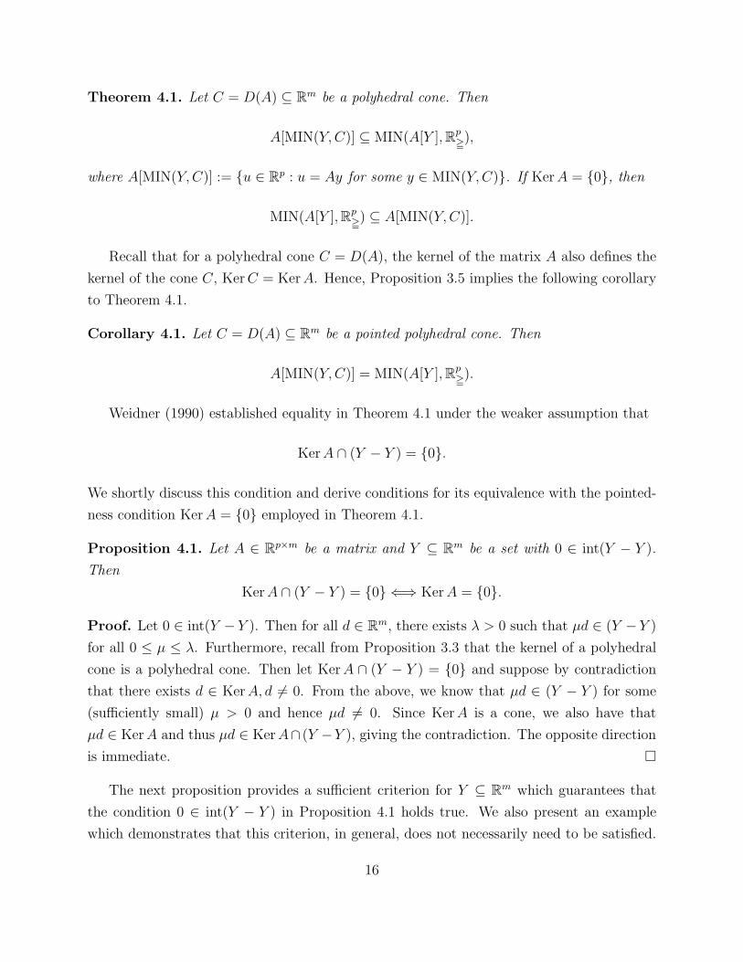
Theorem 4.1. Let C = D(A) ⊆ Rm be a polyhedral cone. Then
A[MIN(Y,C)] ⊆ MIN(A[Y ], Rp=),
where A[MIN(Y,C)] := {u ∈ Rp : u = Ay for some y ∈ MIN(Y,C)}. If Ker A = {0}, then
MIN(A[Y ], Rp=) ⊆ A[MIN(Y,C)].
Recall that for a polyhedral cone C = D(A), the kernel of the matrix A also defines the
kernel of the cone C, Ker C = Ker A. Hence, Proposition 3.5 implies the following corollary
to Theorem 4.1.
Corollary 4.1. Let C = D(A) ⊆ Rm be a pointed polyhedral cone. Then
A[MIN(Y,C)] = MIN(A[Y ], Rp=).
Weidner (1990) established equality in Theorem 4.1 under the weaker assumption that
Ker A ∩ (Y − Y ) = {0}.
We shortly discuss this condition and derive conditions for its equivalence with the pointed-
ness condition Ker A = {0} employed in Theorem 4.1.
Proposition 4.1. Let A ∈ Rp×m be a matrix and Y ⊆ Rm be a set with 0 ∈ int(Y − Y ).
Then
Ker A ∩ (Y − Y ) = {0} ⇐⇒ Ker A = {0}.
Proof. Let 0 ∈ int(Y − Y ). Then for all d ∈ Rm, there exists λ > 0 such that µd ∈ (Y − Y )
for all 0 ≤ µ ≤ λ. Furthermore, recall from Proposition 3.3 that the kernel of a polyhedral
cone is a polyhedral cone. Then let Ker A ∩ (Y − Y ) = {0} and suppose by contradiction
that there exists d ∈ Ker A, d 6= 0. From the above, we know that µd ∈ (Y − Y ) for some
(sufficiently small) µ > 0 and hence µd 6= 0. Since Ker A is a cone, we also have that
µd ∈ Ker A and thus µd ∈ Ker A∩ (Y −Y ), giving the contradiction. The opposite direction
is immediate. ¤
The next proposition provides a sufficient criterion for Y ⊆ Rm which guarantees that
the condition 0 ∈ int(Y − Y ) in Proposition 4.1 holds true. We also present an example
which demonstrates that this criterion, in general, does not necessarily need to be satisfied.
16
Proposition 4.2. If the set Y ⊆ Rm has a nonempty interior, int Y 6= ∅, then
0 ∈ int(Y − Y ).
Proof. Let y ∈ int Y . Then, for all d ∈ Rm, there exists λ > 0 such that y + µd ∈ Y for all
0 ≤ µ ≤ λ. It follows that for all d ∈ Rm, (y + µd − y) = µd ∈ (Y − Y ) for all λ ≥ µ ≥ 0
and hence 0 ∈ int(Y − Y ). ¤
From the above, it can be concluded that Weidner’s condition is equivalent with the point-
edness of the ordering cone for continuous problems in which the set Y is connected and has
nonempty interior, but might provide a true generalization for discrete vector optimization
problems.
In addition, it turns out that the statement of Proposition 4.2 and thus the equivalence
in Proposition 4.1 may also hold true for a set Y whose interior is empty, as illustrated by
the following example.
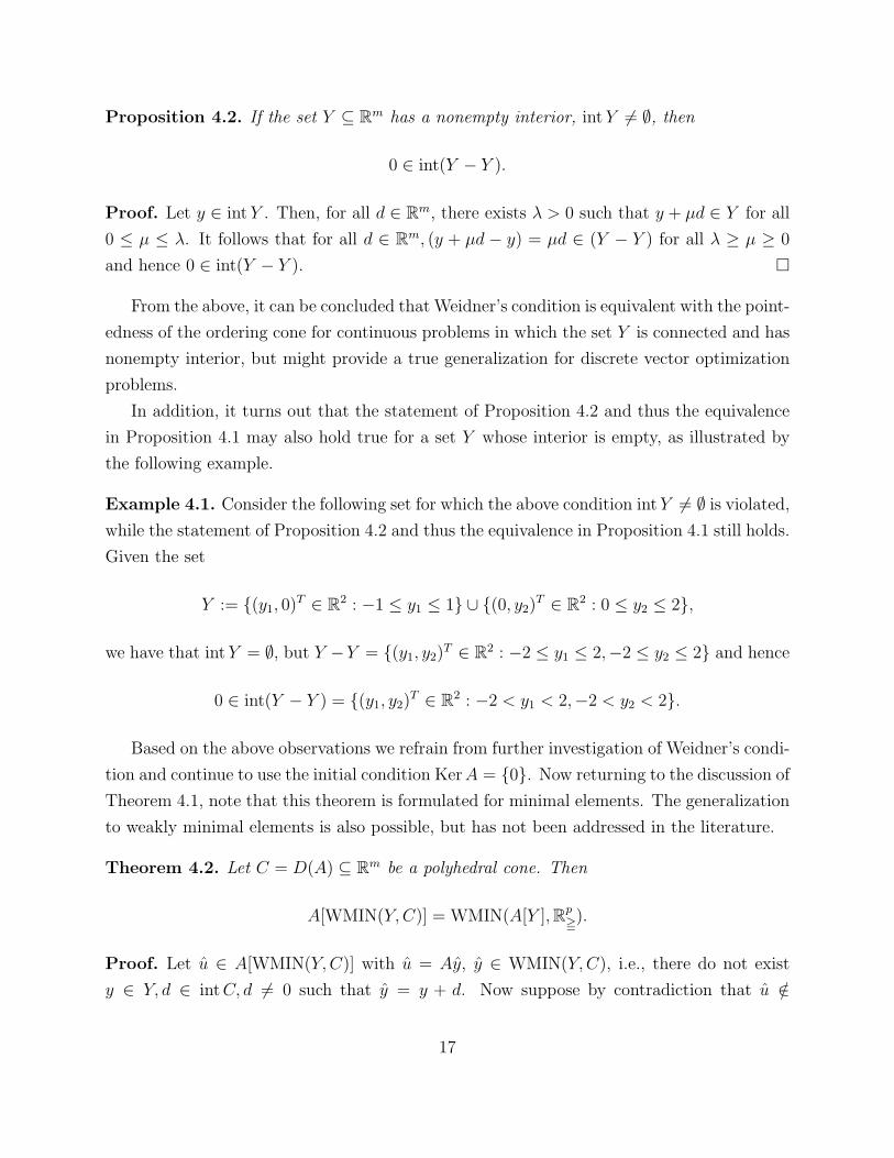
Example 4.1. Consider the following set for which the above condition intY 6= ∅ is violated,
while the statement of Proposition 4.2 and thus the equivalence in Proposition 4.1 still holds.
Given the set
Y := {(y1, 0)T ∈ R2 : −1 ≤ y1 ≤ 1} ∪ {(0, y2)T ∈ R2 : 0 ≤ y2 ≤ 2},
we have that int Y = ∅, but Y −Y = {(y1, y2)T ∈ R2 : −2 ≤ y1 ≤ 2,−2 ≤ y2 ≤ 2} and hence
0 ∈ int(Y − Y ) = {(y1, y2)T ∈ R2 : −2 < y1 < 2,−2 < y2 < 2}.
Based on the above observations we refrain from further investigation of Weidner’s condi-
tion and continue to use the initial condition KerA = {0}. Now returning to the discussion of
Theorem 4.1, note that this theorem is formulated for minimal elements. The generalization
to weakly minimal elements is also possible, but has not been addressed in the literature.
Theorem 4.2. Let C = D(A) ⊆ Rm be a polyhedral cone. Then
A[WMIN(Y,C)] = WMIN(A[Y ], Rp=).
Proof. Let u ∈ A[WMIN(Y,C)] with u = Ay, y ∈ WMIN(Y,C), i.e., there do not exist
y ∈ Y, d ∈ int C, d 6= 0 such that y = y + d. Now suppose by contradiction that u /∈
17
WMIN(A[Y ], Rp=), then u > u for some u ∈ A[Y ], u = Ay, where y ∈ Y, y 6= y. It follows
that
u − u = Ay − Ay = A(y − y) > 0,
and setting d = y − y gives y = y + d, d ∈ int C, d 6= 0 in contradiction to the above. For
the opposite direction, let u ∈ WMIN(A[Y ], Rp=) with u = Ay, y ∈ Y . Then there does not
exist y ∈ Y such that Ay > Ay and hence A(y − y) > 0. Now suppose by contradiction
that u /∈ A[WMIN(Y,C)], or y /∈ WMIN(Y,C). Then there exist y ∈ Y, d ∈ int C such that
y = y + d and hence
A(y − y) = Ad > 0.
This yields the contradiction. ¤
Note that this result can also be derived from Corollary 4.1. First, recall from Definition
2.4 that WMIN(Y,C) = MIN(Y, int C) and then observe that int C is always pointed for
C ⊂ Rm a polyhedral cone, and clearly MIN(Y,C) = WMIN(Y,C) = ∅ for C = Rm and Y
not a singleton.
4.2 Epsilon-minimal elements and polyhedral translated cones
In this section, we derive various generalizations of Theorems 4.1 and 4.2. In its original
formulation restricted to minimal elements with respect to polyhedral cones, we derive the
corresponding results for minimal elements with respect to arbitrary polyhedral sets and, as
a special case, for ε-minimal elements with respect to polyhedral translated cones.
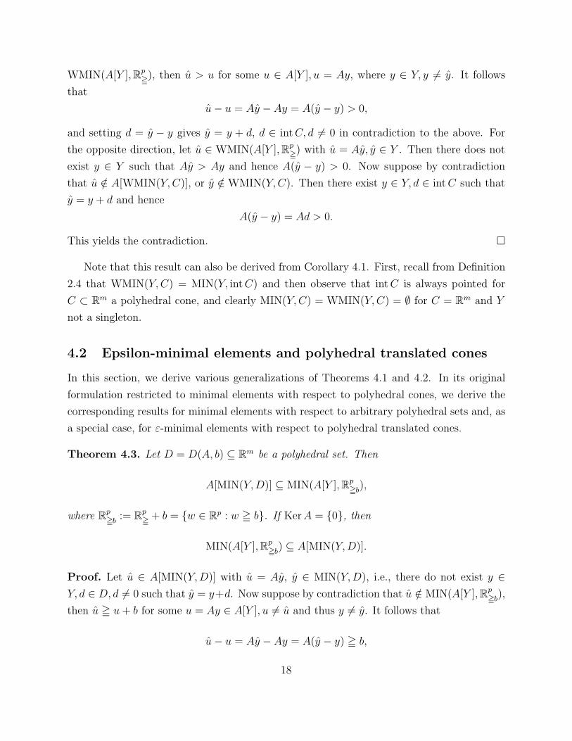
Theorem 4.3. Let D = D(A, b) ⊆ Rm be a polyhedral set. Then
A[MIN(Y,D)] ⊆ MIN(A[Y ], Rp=b
),
where Rp=b
:= Rp= + b = {w ∈ Rp : w = b}. If Ker A = {0}, then
MIN(A[Y ], Rp=b
) ⊆ A[MIN(Y,D)].
Proof. Let u ∈ A[MIN(Y,D)] with u = Ay, y ∈ MIN(Y,D), i.e., there do not exist y ∈Y, d ∈ D, d 6= 0 such that y = y+d. Now suppose by contradiction that u /∈ MIN(A[Y ], Rp
=b),
then u = u + b for some u = Ay ∈ A[Y ], u 6= u and thus y 6= y. It follows that
u − u = Ay − Ay = A(y − y) = b,
18
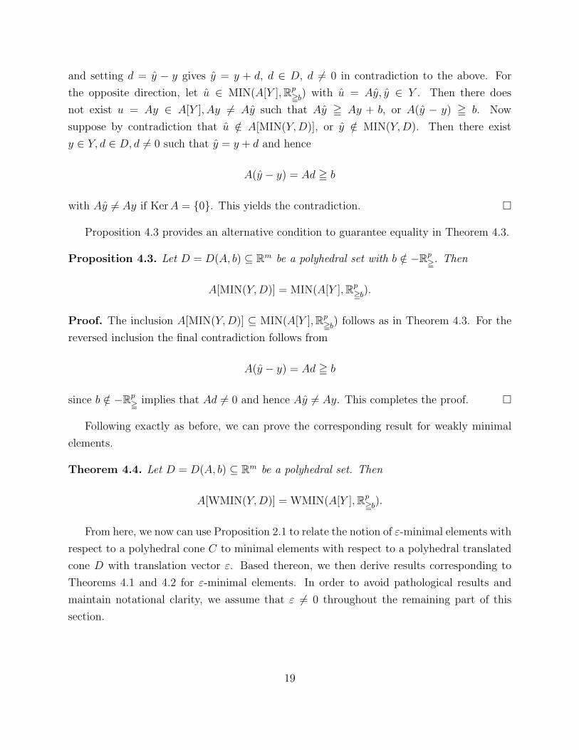
and setting d = y − y gives y = y + d, d ∈ D, d 6= 0 in contradiction to the above. For
the opposite direction, let u ∈ MIN(A[Y ], Rp=b
) with u = Ay, y ∈ Y . Then there does
not exist u = Ay ∈ A[Y ], Ay 6= Ay such that Ay = Ay + b, or A(y − y) = b. Now
suppose by contradiction that u /∈ A[MIN(Y,D)], or y /∈ MIN(Y,D). Then there exist
y ∈ Y, d ∈ D, d 6= 0 such that y = y + d and hence
A(y − y) = Ad = b
with Ay 6= Ay if Ker A = {0}. This yields the contradiction. ¤
Proposition 4.3 provides an alternative condition to guarantee equality in Theorem 4.3.
Proposition 4.3. Let D = D(A, b) ⊆ Rm be a polyhedral set with b /∈ −Rp=. Then
A[MIN(Y,D)] = MIN(A[Y ], Rp=b
).
Proof. The inclusion A[MIN(Y,D)] ⊆ MIN(A[Y ], Rp=b
) follows as in Theorem 4.3. For the
reversed inclusion the final contradiction follows from
A(y − y) = Ad = b
since b /∈ −Rp= implies that Ad 6= 0 and hence Ay 6= Ay. This completes the proof. ¤
Following exactly as before, we can prove the corresponding result for weakly minimal
elements.
Theorem 4.4. Let D = D(A, b) ⊆ Rm be a polyhedral set. Then
A[WMIN(Y,D)] = WMIN(A[Y ], Rp=b
).
From here, we now can use Proposition 2.1 to relate the notion of ε-minimal elements with
respect to a polyhedral cone C to minimal elements with respect to a polyhedral translated
cone D with translation vector ε. Based thereon, we then derive results corresponding to
Theorems 4.1 and 4.2 for ε-minimal elements. In order to avoid pathological results and
maintain notational clarity, we assume that ε 6= 0 throughout the remaining part of this
section.
19
Lemma 4.1. Given a matrix A ∈ Rp×m and a vector ε ∈ Rm, set b = Aε and let C = D(A)
be the polyhedral cone and D = D(A, b) be the polyhedral set implied by A and b. Then
MIN(Y,C, ε) = MIN(Y,D) and WMIN(Y,C, ε) = WMIN(Y,D).
Proof. From Theorem 3.1, first observe that under the given assumptions D = Cε, i.e., the
polyhedral set D describes the polyhedral translated cone Cε. Then apply Proposition 2.1
to conclude with the result. ¤
Theorem 4.5. Let C = D(A) ⊆ Rm be a polyhedral cone with matrix A ∈ Rp×m and ε ∈ Rm
a vector. Then
A[MIN(Y,C, ε)] ⊆ MIN(A[Y ], Rp=b
),
where b = Aε. If Ker A = {0}, then
MIN(A[Y ], Rp=b
) ⊆ A[MIN(Y,C, ε)].
In any case
A[WMIN(Y,C, ε)] = WMIN(A[Y ], Rp=b
).
Proof. From Lemma 4.1 we have that MIN(Y,C, ε) = MIN(Y,D) and WMIN(Y,C, ε) =
WMIN(Y,D), where b = Aε and D = D(A, b) is the translated polyhedral cone implied by A
and b = Aε. Thus we obtain that A[MIN(Y,C, ε)] = A[MIN(Y,D)] and A[WMIN(Y,C, ε)] =
A[WMIN(Y,D)], and now Theorems 4.3 and 4.4 give the result. ¤
Finally, we collect two further corollaries to Theorem 4.5.
Corollary 4.2. Let C = D(A) ⊆ Rm be a pointed polyhedral cone. Then
A[MIN(Y,C, ε)] = MIN(A[Y ], Rp=b
).
Proof. Use Theorem 4.5 and Corollary 3.1. ¤
Alternatively, we obtain the same result from Proposition 4.3.
Corollary 4.3. If b = Aε /∈ −Rp=, then
A[MIN(Y,C, ε)] = MIN(A[Y ], Rp=b
).
20
5 Maximizing over the set of epsilon-minimal elements
Over the years, many authors have shown interest in the problem of optimizing over the effi-
cient set of a multiobjective programming problem, see Benson and Sayin (1994), Tu (2000)
and Jorge (2005), among others. Here we consider the particular problem of maximizing
over the set of ε-minimal elements while retaining to the same underlying ordering cone
C. Motivation was provided by Engau and Wiecek (2005a,b) who described applications of
multiobjective programming problems which require the generation of suboptimal solutions
in practical decision making situations.
Now let Z be a topological real linear space, Y ⊆ Z be a given set and C ⊆ Z be a given
ordering cone. Let ε ∈ C◦ be given and as before denote by MIN(Y,C, ε) and WMIN(Y,C, ε)
the sets of all (weakly) ε-minimal elements of Y with respect to C.
Analogously to the definition of minimal elements, we first define the set of (weakly)
maximal elements for a set X ⊆ Z.
Definition 5.1. An element z ∈ Z is called a maximal element of the set X with respect to
the cone C if z ∈ X and if there does not exist a point x ∈ X with x ≥C z, or equivalently
X ∩ (z + C◦) = ∅
The set of all maximal elements of X with respect to the cone C is denoted by MAX(X,C).
The set of weakly maximal elements WMAX(X,C) is defined as the set of all elements z ∈ X
for which there does not exist a point x ∈ X with x >C z,
X ∩ (z + int C◦) = ∅,
or WMAX(X,C) = MAX(X, int C), equivalently.
Remark 5.1. Using Definition 5.1 together with Definitions 2.3 and 2.4, it is easily verified
that MAX(X,C) = MIN(X,−C) and WMAX(X,C) = WMIN(X,−C).
Now the problem of interest is to identify the set of (weakly) maximal elements within
the set of (weakly) ε-minimal elements, that is to find
WMAX(WMIN(Y,C, ε), C).
Although the underlying set of weakly ε-minimal elements is in general unknown and thus
21
an actual optimization over this set in practice not possible, we can provide an alternative
characterization of (at least) a subset of the above set of interest.
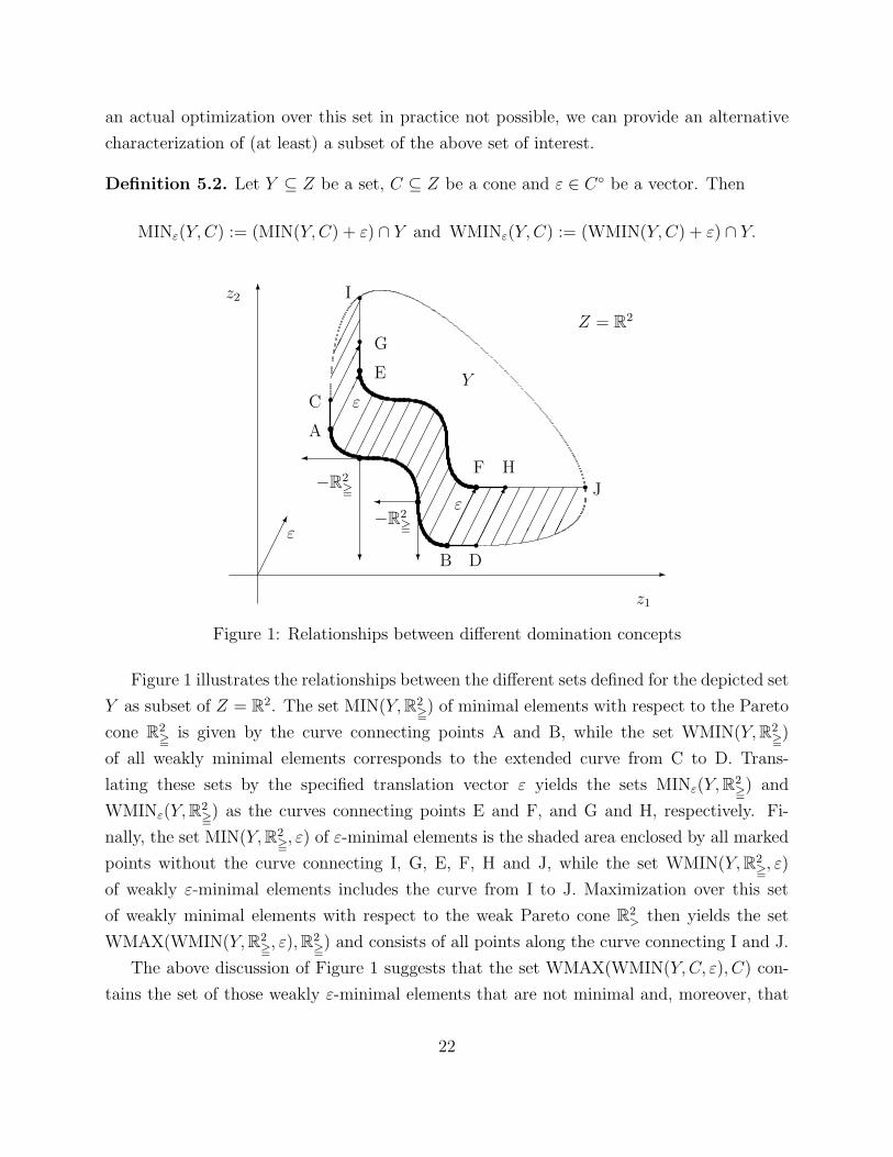
Definition 5.2. Let Y ⊆ Z be a set, C ⊆ Z be a cone and ε ∈ C◦ be a vector. Then
MINε(Y,C) := (MIN(Y,C) + ε) ∩ Y and WMINε(Y,C) := (WMIN(Y,C) + ε) ∩ Y.
-
z1
6z2
sB
sA
rD
rCY
Z = R2
s¾
?
−R2= s¾
?
−R2=
sF
s E
rH
r G
¢¢¢¢
¢¢¢¢
¢¢¢¢
¢¢¢¢ε
rI
r J
¢¢
¢¢
¢¢
¢¢
ε
¢¢¢¢
¢¢¢¢
¢¢¢¢
¢¢¢¢
¢¢¢¢
¢¢¢¢
¢¢¢¢
¢¢¢¢
¢¢¢¢
¢¢¢¢ ¢
¢¢
¢
¢¢
¢¢
¢¢
¢¢
¢¢
¢¢
¢¢
¢¢
¢¢
¢¢
¢¢
¢¢
¢¢
¢¢
¢¢¢¢ε
Figure 1: Relationships between different domination concepts
Figure 1 illustrates the relationships between the different sets defined for the depicted set
Y as subset of Z = R2. The set MIN(Y, R2=) of minimal elements with respect to the Pareto
cone R2= is given by the curve connecting points A and B, while the set WMIN(Y, R2
=)
of all weakly minimal elements corresponds to the extended curve from C to D. Trans-
lating these sets by the specified translation vector ε yields the sets MINε(Y, R2=) and
WMINε(Y, R2=) as the curves connecting points E and F, and G and H, respectively. Fi-
nally, the set MIN(Y, R2=, ε) of ε-minimal elements is the shaded area enclosed by all marked
points without the curve connecting I, G, E, F, H and J, while the set WMIN(Y, R2=, ε)
of weakly ε-minimal elements includes the curve from I to J. Maximization over this set
of weakly minimal elements with respect to the weak Pareto cone R2> then yields the set
WMAX(WMIN(Y, R2=, ε), R2
=) and consists of all points along the curve connecting I and J.
The above discussion of Figure 1 suggests that the set WMAX(WMIN(Y,C, ε), C) con-
tains the set of those weakly ε-minimal elements that are not minimal and, moreover, that
22
this set has the sets MINε(Y,C) and WMINε(Y,C) as (possibly proper) subsets. The verifi-
cation of this intuitive conjecture, however, requires some further preparation.
Lemma 5.1. Let y ∈ WMIN(Y,C) be a weakly minimal element and let y ∈ Y .
(i) If y <C y + ε, then y is an ε-minimal element, y ∈ MIN(Y,C, ε).
(ii) If y 5C y + ε, then y is a weakly ε-minimal element, y ∈ WMIN(Y,C, ε).
Proof. We know y ∈ WMIN(Y,C), so there does not exist y ∈ Y such that y <C y, or
y <C (y + ε) − ε. Then we have for (i), if y <C y + ε, that there does not exist y ∈ Y such
that y 5C y − ε, and hence y is an ε-minimal element. Similarly for (ii), if y 5C y + ε,
we obtain that there does not exist y ∈ Y such that y <C y − ε, and hence y is a weakly
ε-minimal element. ¤
Now the main result consists of two parts.
Theorem 5.1. Let Y ⊆ Z a set, C ⊆ Z a cone and ε ∈ C◦ be given. Then
MINε(Y,C) ⊆ WMINε(Y,C) ⊆ WMIN(Y,C, ε) \ MIN(Y,C, ε).
Proof. The first inclusion follows directly from Definition 5.2. For the second, we ob-
tain that WMINε(Y,C) ⊆ WMIN(Y,C, ε) from Lemma 5.1(ii), and then WMINε(Y,C) ∩MIN(Y,C, ε) = ∅ follows since ε ∈ C◦ is a dominated direction. ¤
While Theorem 5.1 follows under quite general conditions, the second part requires some
further assumptions, namely convexity and pointedness of the underlying cone C.
Theorem 5.2. Let Y ⊆ Z a set, C ⊆ Z an ordering cone and ε ∈ C◦ be given. Then
WMIN(Y,C, ε) \ MIN(Y,C, ε) ⊆ WMAX(WMIN(Y,C, ε), C).
Proof. Let y ∈ WMIN(Y,C, ε) \ MIN(Y,C, ε), then there do not exist y ∈ Y, d ∈ int C
(d 6= −ε as ε ∈ C◦ where C is pointed) such that y = y + d + ε, but y = y + d + ε for
some y ∈ Y and d ∈ C. We have to show that y ∈ WMAX(WMIN(Y,C, ε), C), or that
there do not exist y ∈ WMIN(Y,C, ε), d ∈ int C, d 6= 0 such that y = y − d. Therefore,
suppose by contradiction that y = y − d with y ∈ Y , d ∈ int C, d 6= 0 and show that
y /∈ WMIN(Y,C, ε). From the above, we have y = y + d+ ε with y ∈ Y and d ∈ C, and thus
we obtain y = y + d + d + ε with y ∈ Y and ¯d = d + d ∈ int C as C is convex, with ¯d 6= −ε
again since ε ∈ C◦ with C pointed. Hence, y /∈ WMIN(Y,C, ε), and the proof is complete.
¤
23
Combining Theorem 5.1 and Theorem 5.2 now implies the concluding result.
Corollary 5.1. Let Y ⊆ Z a set, C ⊆ Z an ordering cone and ε ∈ C◦ be given. Then
MINε(Y,C) ⊆ WMINε(Y,C) ⊆ WMIN(Y,C, ε)\MIN(Y,C, ε) ⊆ WMAX(WMIN(Y,C, ε), C).
An application of this result is given in Engau and Wiecek (2005a).
6 Conclusions
In this paper, we study approximate solutions in real-vector optimization and propose the
formal framework of cones for their characterization.
It is well established that minimal elements among a set of vectors can be defined with
respect to some partial order induced upon introduction of an underlying ordering cone.
In direct generalization, approximate solutions are defined as epsilon-minimal elements and
give rise to a number of interesting and previously unaddressed research questions.
At first, realizing that the cones describing epsilon-minimal elements must be shifted from
the origin, preliminary results on translated cones are reported and deal primarily with the
uniqueness of their representation. As a special case of interest, we investigate the possibility
of describing a given polyhedral translated cone by a system of linear inequalities and, from
a reversed point of view, derive conditions for which a given system defines a polyhedral
translated cone. We also mention how these results relate to and extend certain concepts
from linear algebra and convex analysis.
In spite of the theoretical analogy of allowing arbitrary ordering cones, most practical
applications adopt the Pareto order and hence motivate efforts to find relationships between
minimal elements with respect to the Pareto and more general ordering cones. Very satisfying
results have been established for polyhedral cones for which the set of minimal elements can
be transformed into a set of minimal elements with respect to a Pareto cone. Restricted
to minimal elements with respect to polyhedral cones, we derive the corresponding results
for minimal elements with respect to arbitrary polyhedral sets and, as a special case, for
epsilon-minimal elements with respect to polyhedral translated cones.
We hope that these results enable and stimulate further investigation of approximate
solutions within the rigorous formal framework proposed in this paper.
As one such particular research question of interest and directly motivated by parallel
methodological developments in Engau and Wiecek (2005a), we finally address the general
24
problem of optimizing over the set of minimal or epsilon-minimal elements, or more precisely,
the identification of (weakly) maximal elements among the set of (weakly) epsilon-minimal
elements. Facing the challenge that for most practical situations the latter is not given
explicitly and hence that actual optimization is in general not possible, we offer an alternative
characterization of these maximal elements which as a by-product leads to an insightful result
relating epsilon-minimal and weakly epsilon-minimal elements.
While parts of this research have already been put in practice for our personal work,
we believe that some of the results presented in this paper also continue to be of inter-
est and benefit to others for further use and study of approximate solutions in real-vector
optimization problems.
References
Bauschke, H. H. (2003). Duality for Bregman projections onto translated cones and affine
subspaces. Journal of Approximation Theory, 121(1):1–12.
Benson, H. P. and Sayin, S. (1994). Optimization over the efficient set: four special cases.
Journal of Optimization Theory and Applications, 80(1):3–18.
Bergstresser, K., Charnes, A., and Yu, P. L. (1976). Generalization of domination structures
and nondominated solutions in multicriteria decision making. Journal of Optimization
Theory and Applications, 18(1):3–13. Differential game issue.
Bergstresser, K. and Yu, P. L. (1977). Domination structures and multicriteria problems in
N -person games. Theory and Decision, 8(1):5–48. Game theory and conflict resolution, I.
Borwein, J. M. (1983). On the existence of Pareto efficient points. Mathematics of Operations
Research, 8:64–73.
Cambini, A., Luc, D. T., and Martein, L. (2003). Order-preserving transformations and
applications. Journal of Optimization Theory and Applications, 118(2):275–293.
Chen, G. Y. and Yang, X. Q. (2002). Characterizations of variable domination structures via
nonlinear scalarization. Journal of Optimization Theory and Applications, 112(1):97–110.
Chew, K. L. (1979). Domination structures in abstract spaces. In Proceedings of the First
Franco-Southeast Asian Mathematical Conference (Singapore, 1979), Vol. II, pages 190–
204.
25
Corley, H. (1980). An existence result for maximizations with respect to cones. Journal of
Optimization Theory and Applications, 31:277–281.
Deng, S. (1997). On approximate solutions in convex vector optimization. SIAM Journal
on Control and Optimization, 35(6):2128–2136.
Deng, S. (1998). On efficient solutions in vector optimization. Journal of Optimization
Theory and Applications, 96(1):201–209.
Dutta, J. and Vetrivel, V. (2001). On approximate minima in vector optimization. Numerical
Functional Analysis and Optimization, 22(7-8):845–859.
Edgeworth, F. Y. (1881). Mathematical Psychics: An essay on the application of mathematics
to the moral sciences. P. Keagan, London, England.
Engau, A. and Wiecek, M. M. (2005a). Exact generation of epsilon-
efficient solutions in multiple objective programming. Technical Report
TR2005 10 EWa, Department of Mathematical Sciences, Clemson University.
Http://www.math.clemson.edu/reports/TR2005 10 EWa. Submitted for publication.
Engau, A. and Wiecek, M. M. (2005b). Generating epsilon-efficient solutions in multiob-
jective programming. Technical Report TR2005 10 EWb, Department of Mathematical
Sciences, Clemson University. Http://www.math.clemson.edu/reports/TR2005 10 EWb.
European Journal of Operational Research, in print.
Hartley, R. (1978). On cone-efficiency, cone-convexity and cone-compactness. SIAM Journal
on Applied Mathematics, 34:211–222.
Helbig, S. and Pateva, D. (1994). On several concepts for ε-efficiency. OR Spektrum,
16(3):179–186.
Hunt, B. J. (2004). Multiobjective Programming with Convex Cones: Methodology and Ap-
plications. PhD thesis, Clemson University, Clemson, South Carolina, USA. Margaret M.
Wiecek, advisor.
Hunt, B. J. and Wiecek, M. M. (2003). Cones to aid decision making in multicriteria
programming. In Tanino, T., Tanaka, T., and Inuiguchi, M., editors, Multi-Objective
Programming and Goal Programming, pages 153–158. Springer-Verlag, Berlin.
26
Jorge, J. M. (2005). A bilinear algorithm for optimizing a linear function over the efficient
set of a multiple objective linear programming problem. Journal of Global Optimization,
31(1):1–16.
Kazmi, K. R. (2001). Existence of ε-minima for vector optimization problems. Journal of
Optimization Theory and Applications, 109(3):667–674.
Lemaire, B. (1992). Approximation in multiobjective optimization. Journal of Global Opti-
mization, 2(2):117–132.
Li, Z. and Wang, S. (1998). ε-approximate solutions in multiobjective optimization. Opti-
mization, 44(2):161–174.
Lin, S. A. Y. (1976). A comparison of Pareto optimality and domination structure. Metroe-
conomica, 28(1-3):62–74.
Liu, J. C. (1996). ε-Pareto optimality for nondifferentiable multiobjective programming via
penalty function. Journal of Mathematical Analysis and Applications, 198(1):248–261.
Loridan, P. (1984). ε-solutions in vector minimization problems. Journal of Optimization
Theory and Applications, 43(2):265–276.
Loridan, P., Morgan, J., and Raucci, R. (1999). Convergence of minimal and approximate
minimal elements of sets in partially ordered vector spaces. Journal of Mathematical
Analysis and Applications, 239(2):427–439.
Luenberger, D. G. (1969). Optimization by Vector Space Methods (Series in Decision and
Control). New York-London. Sydney-Toronto: John Wiley and Sons, Inc.
Miettinen, K. and Makela, M. M. (2000). Tangent and normal cones in nonconvex multi-
objective optimization. In Research and Practice in Multiple Criteria Decision Making
(Charlottesville, VA, 1998), volume 487 of Lecture Notes in Economics and Mathematical
Systems, pages 114–124. Springer, Berlin.
Miettinen, K. and Makela, M. M. (2001). On cone characterizations of weak, proper and
Pareto optimality in multiobjective optimization. Mathematical Methods of Operations
Research, 53(2):233–245.
Nachbin, L. (1996). Convex sets, convex cones, affine spaces and affine cones. Revista
Colombiana de Matematicas, 30(1):1–23.
27
Nemeth, A. B. (1989). Between Pareto efficiency and Pareto ε-efficiency. Optimization,
20(5):615–637.
Pareto, V. (1896). Cours d’Economie Politique. Rouge, Lausanne, Switzerland.
Rockafellar, R. T. (1970). Convex Analysis. Princeton, N. J.: Princeton University Press.
Rong, W. D. and Wu, Y. N. (2000). ε-weak minimal solutions of vector optimization problems
with set-valued maps. Journal of Optimization Theory and Applications, 106(3):569–579.
Ruzika, S. and Wiecek, M. M. (2005). Approximation methods in multiobjective program-
ming. Journal of Optimization Theory and Applications, 126(3):473–501.
Sawaragi, Y., Nakayama, H., and Tanino, T. (1985). Theory of Multiobjective Optimization,
volume 176 of Mathematics in Science and Engineering. Academic Press Inc., Orlando,
FL.
Sonntag, Y. and Zalinescu, C. (2000). Comparison of existence results for efficient points.
Journal of Optimization Theory and Applications, 105(1):161–188.
Takeda, E. and Nishida, T. (1980). Multiple criteria decision problems with fuzzy domination
structures. Fuzzy Sets and Systems, 3(2):123–136.
Tanaka, T. (1996). Approximately efficient solutions in vector optimization. Journal of
Multi-Criteria Decision Analysis, 5(4):271–278.
Tu, T. V. (2000). Optimization over the efficient set of a parametric multiple objective linear
programming problem. European Journal of Operational Research, 122(3):570–583.
Valyi, I. (1985). Approximate solutions of vector optimization problems. In Systems Analysis
and Simulation 1985, I (Berlin, 1985), volume 27 of Mathematical Research, pages 246–
250. Akademie-Verlag, Berlin.
Weidner, P. (1985). Dominanzmengen und Optimalitatsbegriffe in der Vektoroptimierung.
(Domination sets and optimality conditions in vector optimization theory). Wis-
senschaftliche Zeitschrift der Technischen Hochschule Ilmenau, 31(2):133–146.
Weidner, P. (1987). On interdependencies between objective functions and dominance sets
in vector optimization. In 19. Jahrestagung “Mathematische Optimierung” (Sellin, 1987),
volume 90 of Seminarberichte, pages 136–145. Humboldt Univ. Berlin.
28
Weidner, P. (1990). Complete efficiency and interdependencies between objective functions
in vector optimization. Zeitschrift fur Operations Research. Mathematical Methods of
Operations Research, 34(2):91–115.
Weidner, P. (2003). Tradeoff directions and dominance sets. In Multi-Objective Programming
and Goal Programming, Advances in Soft Computing, pages 275–280. Springer, Berlin.
White, D. J. (1986). Epsilon efficiency. Journal of Optimization Theory and Applications,
49(2):319–337.
Wierzbicki, A. P. (1986). On the completeness and constructiveness of parametric charac-
terizations to vector optimization problems. OR Spektrum, 8(2):73–87.
Wu, H. C. (2004). A solution concept for fuzzy multiobjective programming problems based
on convex cones. Journal of Optimization Theory and Applications, 121(2):397–417.
Yokoyama, K. (1992). ε-optimality criteria for convex programming problems via exact
penalty functions. Mathematical Programming, 56(2, Ser. A):233–243.
Yokoyama, K. (1994). ε-optimality criteria for vector minimization problems via exact
penalty functions. Journal of Mathematical Analysis and Applications, 187(1):296–305.
Yokoyama, K. (1996). Epsilon approximate solutions for multiobjective programming prob-
lems. Journal of Mathematical Analysis and Applications, 203(1):142–149.
Yokoyama, K. (1999). Relationships between efficient set and ε-efficient set. In Nonlinear
Analysis and Convex Analysis (Niigata, 1998), pages 376–380. World Sci. Publishing,
River Edge, NJ.
Yu, P. L. (1974). Cone convexity, cone extreme points, and nondominated solutions in
decision problems with multiobjectives. Journal of Optimization Theory and Applications,
14:319–377.
Yu, P.-L. (1985). Multiple-Criteria Decision Making. Concepts, Techniques, and Extensions.
Mathematical Concepts and Methods in Science and Engineering, 30. New York-London:
Plenum Press.
29