Conformal Mappings inGeometric AlgebraGarret Sobczyk

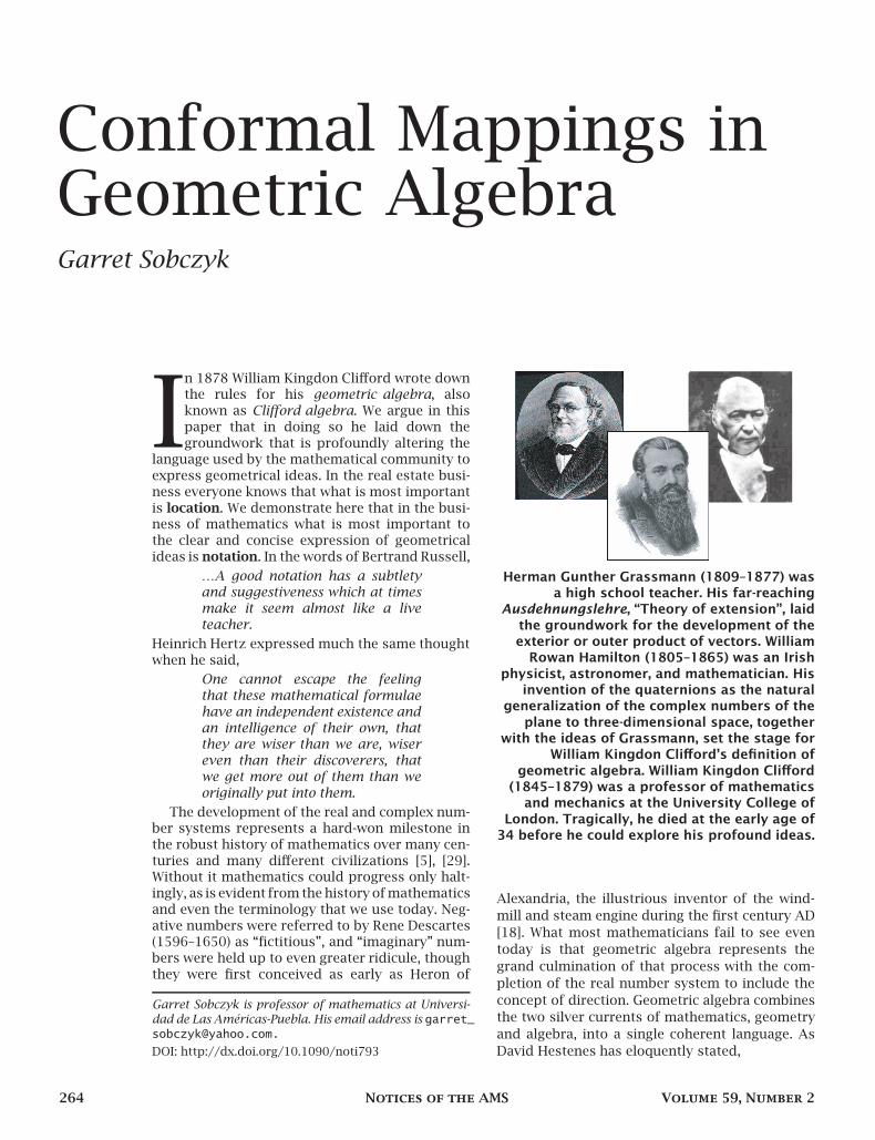
In 1878 William Kingdon Clifford wrote downthe rules for his geometric algebra, alsoknown as Clifford algebra. We argue in thispaper that in doing so he laid down thegroundwork that is profoundly altering the

language used by the mathematical community toexpress geometrical ideas. In the real estate busi-ness everyone knows that what is most importantis location. We demonstrate here that in the busi-ness of mathematics what is most important tothe clear and concise expression of geometricalideas is notation. In the words of Bertrand Russell,

…A good notation has a subtletyand suggestiveness which at timesmake it seem almost like a liveteacher.

Heinrich Hertz expressed much the same thoughtwhen he said,

One cannot escape the feelingthat these mathematical formulaehave an independent existence andan intelligence of their own, thatthey are wiser than we are, wisereven than their discoverers, thatwe get more out of them than weoriginally put into them.

The development of the real and complex num-ber systems represents a hard-won milestone inthe robust history of mathematics over many cen-turies and many different civilizations [5], [29].Without it mathematics could progress only halt-ingly, as is evident from the history of mathematicsand even the terminology that we use today. Neg-ative numbers were referred to by Rene Descartes(1596–1650) as “fictitious”, and “imaginary” num-bers were held up to even greater ridicule, thoughthey were first conceived as early as Heron of

Garret Sobczyk is professor of mathematics at Universi-

dad de Las Américas-Puebla. His email address is garret_

sobczyk@yahoo.com.

DOI: http://dx.doi.org/10.1090/noti793

Herman Gunther Grassmann (1809–1877) wasa high school teacher. His far-reaching

Ausdehnungslehre, “Theory of extension”, laidthe groundwork for the development of theexterior or outer product of vectors. William

Rowan Hamilton (1805–1865) was an Irishphysicist, astronomer, and mathematician. His

invention of the quaternions as the naturalgeneralization of the complex numbers of the

plane to three-dimensional space, togetherwith the ideas of Grassmann, set the stage for

William Kingdon Clifford’s definition ofgeometric algebra. William Kingdon Clifford

(1845–1879) was a professor of mathematicsand mechanics at the University College of

London. Tragically, he died at the early age of34 before he could explore his profound ideas.

Alexandria, the illustrious inventor of the wind-

mill and steam engine during the first century AD

[18]. What most mathematicians fail to see even

today is that geometric algebra represents the

grand culmination of that process with the com-

pletion of the real number system to include the

concept of direction. Geometric algebra combines

the two silver currents of mathematics, geometry

and algebra, into a single coherent language. As

David Hestenes has eloquently stated,

264 Notices of the AMS Volume 59, Number 2

Algebra without geometry is blind,

geometry without algebra is dumb.

David Hestenes, a newly hired assistant profes-

sor of physics, introduced me to geometric algebra

at Arizona State University in 1966. I immediatelybecame captivated by the idea that geometric al-

gebra is the natural completion of the real number

system to include the concept of direction. If thisidea is correct, it should be possible to formulate

all the ideas of multilinear linear algebra, tensor

analysis, and differential geometry. I consideredit to be a major breakthrough when I succeeded

in proving the fundamental Cayley-Hamilton the-

orem within the framework of geometric algebra.The next task was mastering differential geome-

try. Five years later, with Hestenes as my thesis

director, I completed my doctoral dissertation,

“Mappings of Surfaces in Euclidean Space UsingGeometric Algebra” [26].

Much work of Hestenes and other theoretical

physicists has centered around understanding thegeometric meaning of the appearance of imaginary

numbers in quantum mechanics. Ed Witten, in his

Josiah Willard Gibbs Lecture “Magic, Mystery, andMatrix” says, “Physics without strings is roughly

analogous to mathematics without complex num-

bers” [31]. In a personal communication with theauthor, Witten points out that “Pierre Ramond, in

1970, generalized the Clifford algebra from field

theory (where Dirac had used it) to string theory.”

Dale Husemöller in his book Fibre Bundles includesa chapter on Clifford algebras, recognizing their

importance in “topological applications and for

giving a concrete description of the group Spin(n)”[13]. Other mathematicians have developed an ex-

tensive new field which has come to be known as

“Clifford analysis” [3], [7] and “spin geometry” [2].During the academic year 1972–73 I continued

work at Arizona State University with David on dif-

ferential geometry as a visiting assistant professor.The following year, at the height of the academic

crunch, I was on my own—a young unemployed

mathematician, but with a mission: To convincethe world of the importance of geometric algebra. I

travelled to Europe and European universities giv-

ing talks when and where I was graciously invited.

During the year 1973–74, Professor Roman Dudaof the Polish Academy of Sciences offered me a

postgraduate research position, which I gratefully

accepted.My collaboration with David culminated a num-

ber of years later with the publication of our book

Clifford Algebra to Geometric Calculus: A UnifiedLanguage for Mathematics and Physics [11]. Over

the years I have been searching for the best way

to handle ideas in linear algebra and differentialgeometry, particularly with regard to introducing

students to geometric algebra at the undergrad-

uate level. To this end, I have been working

to complete a new manuscript New Foundations

in Mathematics: The Geometric Concept of Num-

bers which has been accepted for publication by

Birkhäuser [24].Distilling geometric algebra down to its core,

it is the extension of the real number system to

include new anticommuting square roots of ±1,which represent mutually orthogonal unit vectors

in successively higher dimensions. Whereas every-

body is familiar with the idea of the imaginarynumber i = √−1, the idea of a new square rootu = √+1 ∉ R has taken longer to be assimilated

into the main body of mathematics. However, in[22] it is shown that the hyperbolic numbers, which

have much in common with their more famous

brothers the complex numbers, also lead to anefficacious solution of the cubic equation.

The time has come for geometric algebra to

become universally recognized for what it is: the

completion of the real number system to includethe concept of direction. Let twenty-first century

mathematics be a century of consolidation and

streamlining so that it can bloom with all therenewed vigor that it will need to prosper in the

future [10].

Fundamental ConceptsLet Rp,q be the pseudoeuclidean space of the

indefinite nondegenerate real quadratic form q(x)

with signature p, q, where x ∈ Rp,q . With this

quadratic form, we define the inner product x · yfor x,y ∈ Rp,q to be

x · y = 1

2[q(x+ y)− q(x)− q(y)].

Let (e)(n) = (e1,e2, . . . ,ep+q) denote the row ofstandard orthonormal anticommuting basis vec-

tors of Rp,q , where e2j = q(ej) for j = 1, . . . , n,

i.e.,

e21 = · · · = e2

p = 1 and e2p+1 = · · · = e2

p+q = −1

and n = p + q. Taking the transpose of the row

of basis vectors (e)(n) gives the column (e)T(n) ofthese same basis vectors. The metric tensor [g] ofRp,q is defined to be the Gramian matrix

(1) [g] := (e)T(n) · (e)(n),which is a diagonal matrix with the first p entries+1 and the remaining entries −1. The standard

reciprocal basis to (e)(n) is then defined, with

raised indices, by

(e)(n) = [g](e)T(n).In terms of the standard basis (e)(n), and its re-

ciprocal basis (e)(n), a vector x ∈ Rp,q is efficientlyexpressed by

x = (e)(n)(x)(n) = (x)(n)(e)(n).Both the column vector of components (x)(n) and

the row vector of components of x are, of course,

February 2012 Notices of the AMS 265

Figure 1.

real numbers. If y = (e)(n)(y)(n) is a second suchvector, then the inner product between them is

x · y = (x)(n)(e)(n) · (e)(n)(y)(n)

=n∑

i=1

xiyi =

p∑

i=1

xiyi −n∑

j=p+1

xjyj ,

where n = p + q.Let (a)(n) be a second basis of Rp,q . Then

(2) (a)(n) = (e)(n)A and (a)T(n) = AT (e)T(n),where A is the matrix of transition from the stan-dard basis (e)(n) of Rp,q to the basis (a)(n) of Rp,q .The Gramian matrix of inner products of the basisvectors (a)(n) is then given by

(a)T(n) · (a)(n) = AT (e)T(n) · (e)(n)A = AT [g]Awhere [g] is the metric tensor of Rp,q defined in(1).

The real associative geometric algebra Gp,q =Gp,q(R

p,q) is generated by taking sums of geometricproducts of the vectors in Rp,q, subjected to therule that x2 = q(x) = x · x for all vectors x ∈ Rp,q .The dimension of Gp,q as a real linear space is 2n,where n = p + q, with the standard orthonormalbasis of geometric numbers

Gp,q = spaneλknk=0,

where the

(nk

)k-vector basis elements of the form

eλk are defined by

eλk = ei1 ...ik = ei1 · · ·eik

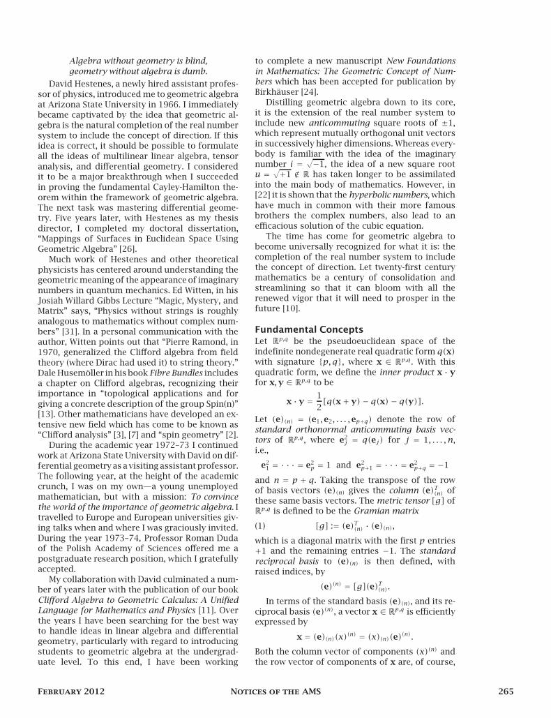
Figure 2. The vector aaa is reflected in thexyxyxy -plane to give the vector b = e12ae12b = e12ae12b = e12ae12, where

e1e1e1 and e2e2e2 are unit vectors along the xxx and yyyaxis, respectively, and e12e12e12 is the unit bivector

of the xyxyxy-plane.

for each λk = i1 . . . ik where 1 ≤ i1 < · · · < ik ≤ n.When k = 0, λ0 = 0 and e0 = 1. For example, the23-dimensional geometric algebraG3 ofR3 has thestandard basis

G3 = spaneλk3k=0

= span1,e1,e2,e3,e12,e13,e23,e123.The geometric numbers of space are pictured inFigure 1.

The great advantage of geometric algebra isthat deep geometrical relationships can be ex-pressed directly in terms of the multivectors ofthe algebra without having to constantly refer toa basis; see Figures 2 and 3. On the other hand,the language gives geometric legs to the power-ful matrix formalism that has developed over thelast one hundred fifty years. As a real associativealgebra, each geometric algebra under geometricmultiplication is isomorphic to a correspondingalgebra or subalgebra of real matrices, and, in-deed, we have advocated elsewhere the need fora uniform approach to both of these structures[23], [27]. Matrices are invaluable for systematizingcalculations, but geometric algebra provides deepgeometrical insight and powerful algebraic toolsfor the efficient expression of geometrical prop-erties. Clifford algebras and their relationships tomatrix algebra and the classical groups have beenthoroughly studied in [15], [21] and elsewhere.

Whereas it is impossible to summarize all ofthe identities in geometric algebra that we needhere, there are many good references that areavailable, for example, [1], [6], [9], [11], [15]. Themost basic identity is the breaking down of thegeometric product of two vectors x,y ∈ Rp,q intothe symmetric and skewsymmetic parts, giving

(3) xy = 1

2(xy+yx)+ 1

2(xy−yx) = x · y+ x∧y,

where the inner product x · y is the symmetricpart and the outer product x∧y is the skewsym-metric part. For whatever the reason, historical orotherwise, the importance of this identity for math-ematics has yet to be fully appreciated. The outer

266 Notices of the AMS Volume 59, Number 2

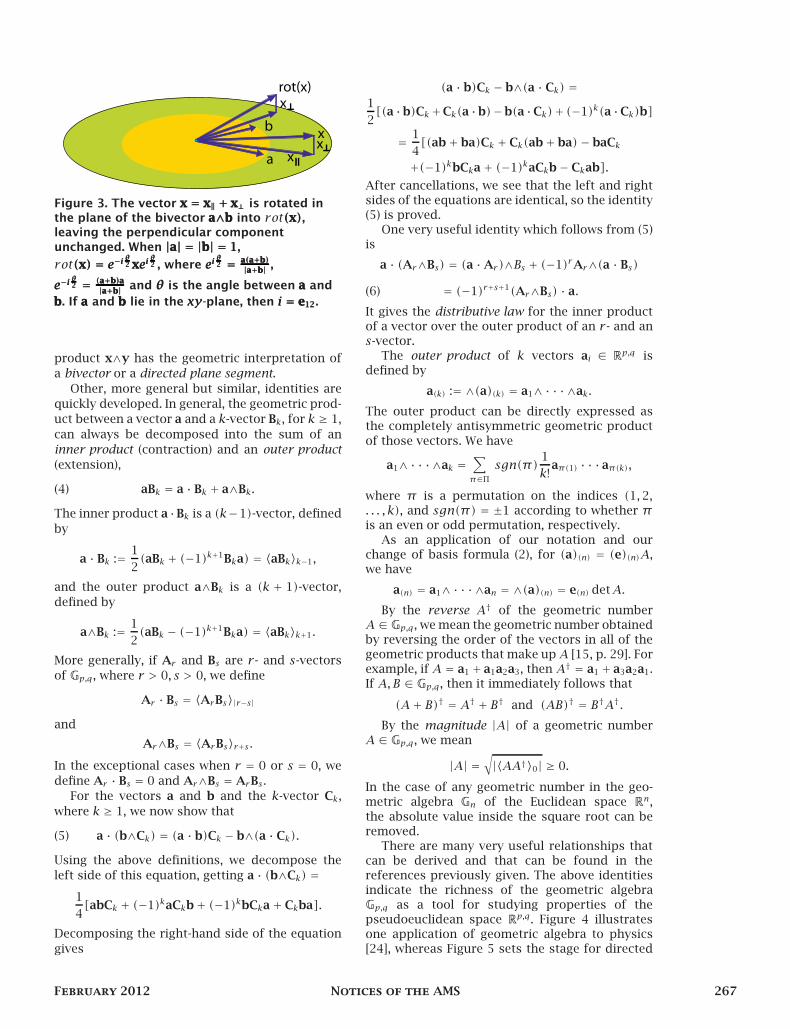
Figure 3. The vector x = x‖ + x⊥x = x‖ + x⊥x = x‖ + x⊥ is rotated inthe plane of the bivector a∧ba∧ba∧b into rot(x)(x)(x),leaving the perpendicular componentunchanged. When |a| = |b| = 1|a| = |b| = 1|a| = |b| = 1,

rot(x) = e−i θ2 xeiθ2(x) = e−i θ2 xeiθ2(x) = e−i θ2 xeiθ2 , where ei

θ2 = a(a+b)

|a+b|eiθ2 = a(a+b)

|a+b|eiθ2 = a(a+b)

|a+b| ,

e−iθ2 = (a+b)a

|a+b|e−iθ2 = (a+b)a

|a+b|e−iθ2 = (a+b)a

|a+b| and θθθ is the angle between aaa and

bbb. If aaa and bbb lie in the xyxyxy-plane, then i = e12i = e12i = e12.

product x∧y has the geometric interpretation of

a bivector or a directed plane segment.

Other, more general but similar, identities are

quickly developed. In general, the geometric prod-

uct between a vector a and a k-vector Bk, for k ≥ 1,

can always be decomposed into the sum of an

inner product (contraction) and an outer product

(extension),

(4) aBk = a · Bk + a∧Bk.

The inner product a ·Bk is a (k−1)-vector, defined

by

a · Bk := 1

2(aBk + (−1)k+1Bka) = 〈aBk〉k−1,

and the outer product a∧Bk is a (k + 1)-vector,

defined by

a∧Bk := 1

2(aBk − (−1)k+1Bka) = 〈aBk〉k+1.

More generally, if Ar and Bs are r - and s-vectors

of Gp,q , where r > 0, s > 0, we define

Ar · Bs = 〈ArBs〉|r−s|and

Ar∧Bs = 〈ArBs〉r+s .In the exceptional cases when r = 0 or s = 0, we

define Ar · Bs = 0 and Ar∧Bs = ArBs .

For the vectors a and b and the k-vector Ck,

where k ≥ 1, we now show that

(5) a · (b∧Ck) = (a · b)Ck − b∧(a · Ck).

Using the above definitions, we decompose the

left side of this equation, getting a · (b∧Ck) =1

4[abCk + (−1)kaCkb+ (−1)kbCka + Ckba].

Decomposing the right-hand side of the equation

gives

(a · b)Ck − b∧(a · Ck) =1

2[(a ·b)Ck+Ck(a ·b)−b(a ·Ck)+ (−1)k(a ·Ck)b]

= 1

4[(ab+ ba)Ck + Ck(ab+ ba)− baCk

+(−1)kbCka + (−1)kaCkb− Ckab].

After cancellations, we see that the left and rightsides of the equations are identical, so the identity(5) is proved.

One very useful identity which follows from (5)is

a · (Ar∧Bs) = (a ·Ar )∧Bs + (−1)rAr∧(a · Bs)

(6) = (−1)r+s+1(Ar∧Bs) · a.

It gives the distributive law for the inner productof a vector over the outer product of an r - and ans-vector.

The outer product of k vectors ai ∈ Rp,q isdefined by

a(k) := ∧(a)(k) = a1∧· · ·∧ak.

The outer product can be directly expressed asthe completely antisymmetric geometric product

of those vectors. We have

a1∧· · ·∧ak =∑

π∈Πsgn(π)

1

k!aπ(1) · · · aπ(k),

where π is a permutation on the indices (1,2,. . . , k), and sgn(π) = ±1 according to whether πis an even or odd permutation, respectively.

As an application of our notation and ourchange of basis formula (2), for (a)(n) = (e)(n)A,we have

a(n) = a1∧·· ·∧an = ∧(a)(n) = e(n) detA.

By the reverse A† of the geometric numberA ∈ Gp,q , we mean the geometric number obtainedby reversing the order of the vectors in all of thegeometric products that make up A [15, p. 29]. Forexample, if A = a1+ a1a2a3, then A† = a1+ a3a2a1.If A,B ∈ Gp,q , then it immediately follows that

(A+ B)† = A† + B† and (AB)† = B†A†.By the magnitude |A| of a geometric number

A ∈ Gp,q , we mean

|A| =√|〈AA†〉0| ≥ 0.

In the case of any geometric number in the geo-metric algebra Gn of the Euclidean space Rn,

the absolute value inside the square root can beremoved.

There are many very useful relationships thatcan be derived and that can be found in thereferences previously given. The above identitiesindicate the richness of the geometric algebraGp,q as a tool for studying properties of thepseudoeuclidean space Rp,q. Figure 4 illustratesone application of geometric algebra to physics[24], whereas Figure 5 sets the stage for directed

February 2012 Notices of the AMS 267

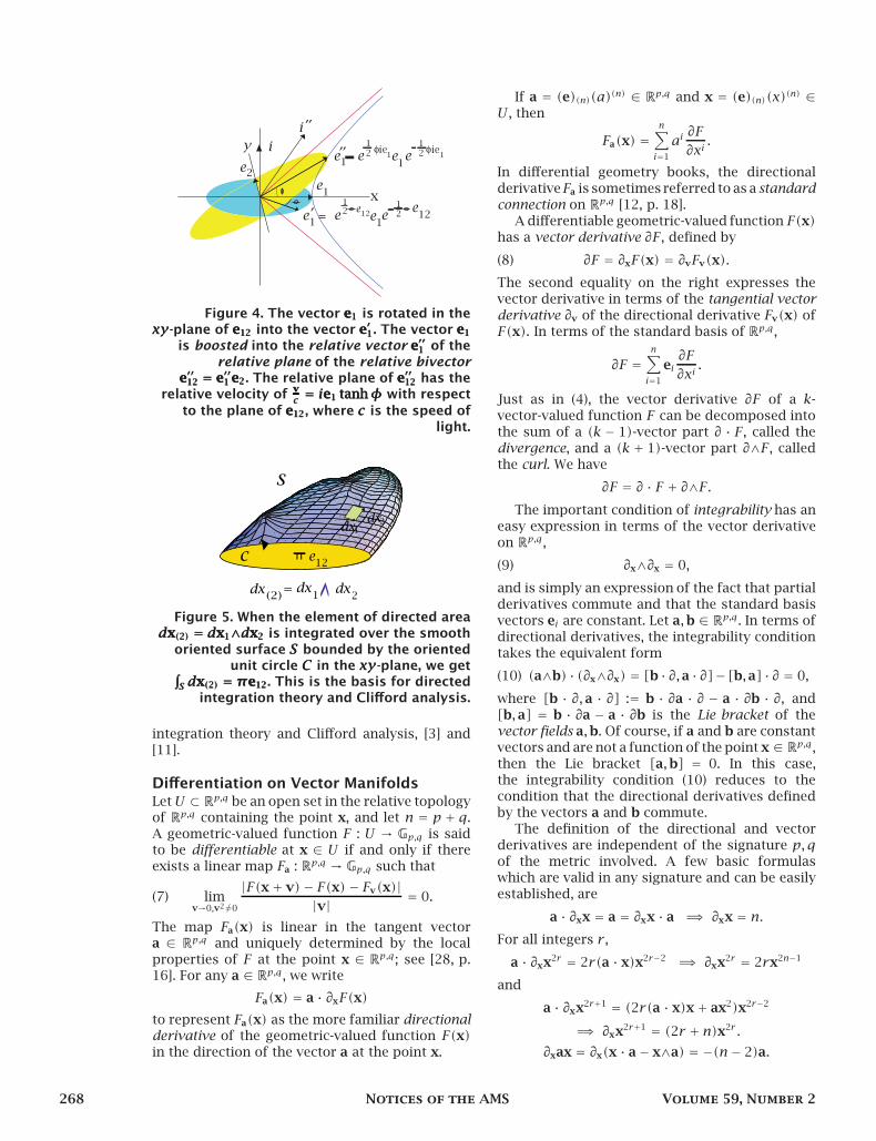
Figure 4. The vector e1e1e1 is rotated in thexyxyxy-plane of e12e12e12 into the vector e′1e′1e′1. The vector e1e1e1

is boosted into the relative vector e′′1e′′1e′′1 of therelative plane of the relative bivector

e′′12 = e′′1 e2e′′12 = e′′1 e2e′′12 = e′′1 e2. The relative plane of e′′12e′′12e′′12 has therelative velocity of

v

c= ie1 tanhφ

v

c= ie1 tanhφv

c= ie1 tanhφ with respect

to the plane of e12e12e12, where ccc is the speed oflight.

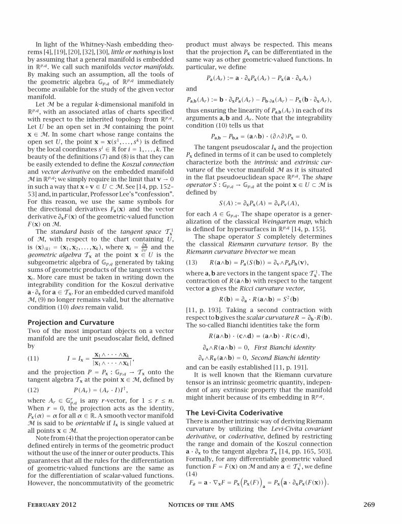
Figure 5. When the element of directed areadx(2) = dx1∧dx2dx(2) = dx1∧dx2dx(2) = dx1∧dx2 is integrated over the smooth

oriented surface SSS bounded by the orientedunit circle CCC in the xyxyxy -plane, we get∫

S dx(2) = πe12

∫S dx(2) = πe12

∫S dx(2) = πe12. This is the basis for directed

integration theory and Clifford analysis.

integration theory and Clifford analysis, [3] and[11].

Differentiation on Vector ManifoldsLetU ⊂ Rp,q be an open set in the relative topologyof Rp,q containing the point x, and let n = p + q.A geometric-valued function F : U → Gp,q is saidto be differentiable at x ∈ U if and only if thereexists a linear map Fa : Rp,q → Gp,q such that

(7) limv→0,v2 6=0

|F(x+ v)− F(x)− Fv(x)||v| = 0.

The map Fa(x) is linear in the tangent vectora ∈ Rp,q and uniquely determined by the localproperties of F at the point x ∈ Rp,q ; see [28, p.16]. For any a ∈ Rp,q , we write

Fa(x) = a · ∂xF(x)

to represent Fa(x) as the more familiar directionalderivative of the geometric-valued function F(x)in the direction of the vector a at the point x.

If a = (e)(n)(a)(n) ∈ Rp,q and x = (e)(n)(x)(n) ∈U , then

Fa(x) =n∑

i=1

ai∂F

∂xi.

In differential geometry books, the directionalderivativeFa is sometimes referred to as a standardconnection on Rp,q [12, p. 18].

A differentiable geometric-valued function F(x)has a vector derivative ∂F , defined by

(8) ∂F = ∂xF(x) = ∂vFv(x).

The second equality on the right expresses thevector derivative in terms of the tangential vectorderivative ∂v of the directional derivative Fv(x) ofF(x). In terms of the standard basis of Rp,q ,

∂F =n∑

i=1

ei∂F

∂xi.

Just as in (4), the vector derivative ∂F of a k-vector-valued function F can be decomposed intothe sum of a (k − 1)-vector part ∂ · F , called thedivergence, and a (k + 1)-vector part ∂∧F , calledthe curl. We have

∂F = ∂ · F + ∂∧F.The important condition of integrability has an

easy expression in terms of the vector derivativeon Rp,q ,

(9) ∂x∧∂x = 0,

and is simply an expression of the fact that partialderivatives commute and that the standard basisvectors ei are constant. Let a,b ∈ Rp,q . In terms ofdirectional derivatives, the integrability conditiontakes the equivalent form

(10) (a∧b) · (∂x∧∂x) = [b ·∂,a ·∂]− [b,a] ·∂ = 0,

where [b · ∂,a · ∂] := b · ∂a · ∂ − a · ∂b · ∂, and[b,a] = b · ∂a − a · ∂b is the Lie bracket of thevector fields a,b. Of course, if a and b are constantvectors and are not a function of the point x ∈ Rp,q ,then the Lie bracket [a,b] = 0. In this case,the integrability condition (10) reduces to thecondition that the directional derivatives definedby the vectors a and b commute.

The definition of the directional and vectorderivatives are independent of the signature p, qof the metric involved. A few basic formulaswhich are valid in any signature and can be easilyestablished, are

a · ∂xx = a = ∂xx · a =⇒ ∂xx = n.For all integers r ,

a · ∂xx2r = 2r(a · x)x2r−2=⇒ ∂xx2r = 2rx2n−1

and

a · ∂xx2r+1 = (2r(a · x)x+ ax2)x2r−2

=⇒ ∂xx2r+1 = (2r + n)x2r .

∂xax = ∂x(x · a− x∧a) = −(n− 2)a.

268 Notices of the AMS Volume 59, Number 2

In light of the Whitney-Nash embedding theo-

rems [4], [19], [20], [32], [30], little or nothing is lostby assuming that a general manifold is embeddedin Rp,q . We call such manifolds vector manifolds.By making such an assumption, all the tools ofthe geometric algebra Gp,q of Rp,q immediatelybecome available for the study of the given vectormanifold.

Let M be a regular k-dimensional manifold inRp,q , with an associated atlas of charts specifiedwith respect to the inherited topology from Rp,q .Let U be an open set in M containing the point

x ∈ M. In some chart whose range contains theopen set U , the point x = x(s1, . . . , sk) is definedby the local coordinates s i ∈ R for i = 1, . . . , k. Thebeauty of the definitions (7) and (8) is that they canbe easily extended to define the Koszul connectionand vector derivative on the embedded manifoldM inRp,q; we simply require in the limit that v → 0in such a way that x+v ∈ U ⊂M. See [14, pp. 152–53] and, in particular, Professor Lee’s “confession”.For this reason, we use the same symbols forthe directional derivatives Fa(x) and the vector

derivative ∂xF(x) of the geometric-valued functionF(x) on M.

The standard basis of the tangent space T 1x

of M, with respect to the chart containing U ,

is (x)(k) = (x1,x2, . . . ,xk), where xi = ∂x

∂siand the

geometric algebra Tx at the point x ∈ U is thesubgeometric algebra of Gp,q generated by takingsums of geometric products of the tangent vectorsxi . More care must be taken in writing down theintegrability condition for the Koszul derivativea·∂x for a ∈ Tx. For an embedded curved manifoldM, (9) no longer remains valid, but the alternative

condition (10) does remain valid.

Projection and CurvatureTwo of the most important objects on a vectormanifold are the unit pseudoscalar field, definedby

(11) I = Ix = x1∧· · ·∧xk

|x1∧· · ·∧xk|,

and the projection P = Px : Gp,q → Tx onto thetangent algebra Tx at the point x ∈M, defined by

(12) P(Ar) = (Ar · I)I†,where Ar ∈ Grp,q is any r -vector, for 1 ≤ r ≤ n.

When r = 0, the projection acts as the identity,Px(α) = α for allα ∈ R. A smooth vector manifoldM is said to be orientable if Ix is single valued atall points x ∈M.

Note from (4) that the projection operator can bedefined entirely in terms of the geometric productwithout the use of the inner or outer products. This

guarantees that all the rules for the differentiationof geometric-valued functions are the same asfor the differentiation of scalar-valued functions.However, the noncommutativity of the geometric

product must always be respected. This means

that the projection Px can be differentiated in the

same way as other geometric-valued functions. Inparticular, we define

Pa(Ar) := a · ∂xPx(Ar )− Px(a · ∂xAr)

and

Pa,b(Ar) := b · ∂xPa(Ar )− Pb·∂a(Ar )− Px(b · ∂xAr),

thus ensuring the linearity of Pa,b(Ar ) in each of itsarguments a,b and Ar . Note that the integrability

condition (10) tells us that

Pa,b − Pb,a = (a∧b) · (∂∧∂)Px = 0.

The tangent pseudoscalar Ix and the projectionPx defined in terms of it can be used to completely

characterize both the intrinsic and extrinsic cur-

vature of the vector manifold M as it is situatedin the flat pseudoeuclidean space Rp,q . The shape

operator S : Gp,q → Gp,q at the point x ∈ U ⊂M is

defined by

S(A) := ∂xPx(A) = ∂vPv(A),

for each A ∈ Gp,q. The shape operator is a gener-

alization of the classical Weingarten map, which

is defined for hypersurfaces in Rp,q [14, p. 155].The shape operator S completely determines

the classical Riemann curvature tensor. By the

Riemann curvature bivector we mean

(13) R(a∧b) = Pa(S(b)) = ∂v∧PaPb(v),

where a,b are vectors in the tangent spaceT 1x . The

contraction of R(a∧b) with respect to the tangent

vector a gives the Ricci curvature vector,

R(b) = ∂a · R(a∧b) = S2(b)

[11, p. 193]. Taking a second contraction with

respect tobgives the scalar curvatureR = ∂b·R(b).The so-called Bianchi identities take the form

R(a∧b) · (c∧d) = (a∧b) · R(c∧d),

∂a∧R(a∧b) = 0, First Bianchi identity

∂v∧R/v(a∧b) = 0, Second Bianchi identity

and can be easily established [11, p. 191].It is well known that the Riemann curvature

tensor is an intrinsic geometric quantity, indepen-

dent of any extrinsic property that the manifoldmight inherit because of its embedding in Rp,q.

The Levi-Civita CoderivativeThere is another intrinsic way of deriving Riemann

curvature by utilizing the Levi-Civita covariant

derivative, or coderivative, defined by restricting

the range and domain of the Koszul connectiona · ∂x to the tangent algebra Tx [14, pp. 165, 503].

Formally, for any differentiable geometric valued

function F = F(x) onM and any a ∈ T 1x , we define

(14)

F/a = a · ∇xF = Px

(Px(F)

)a= Px

(a · ∂xPx(F(x))

).

February 2012 Notices of the AMS 269

We then naturally define the vector coderivative of

F = F(x) by

∇F = ∂vF/v.

The Riemann curvature operator

(a∧b) · (∇x∧∇x)

takes any tangent multivector field A ∈ Tx into

the tangent multivector field R(a∧b)×A, where

R(a∧b)×A := 1

2

(R(a∧b)A−AR(a∧b)

).

We have

(a∧b)·(∇x∧∇x)A(x) =([b·∇,a·∇]−[b,a]·∇

)A

= (PbPa − PaPb)(A) = R(a∧b)×A,where a,b ∈ T 1

x and A = A(x) is any tangent

multivector field with values in the tangent algebra

Tx. For example, for c ∈ Tx, we have, using (13),

R(a∧b) · c = [∂v∧PaPb(c)] · c

= ∂vPaPb(v) · c− PaPb(c) = (PbPa − PaPb)(c).

Mappings between SurfacesWe now come to the heart of this article. Let

f :M→M′, x′ = f (x),be a smooth mapping between two regular k-

surfaces in Rp,q . If x = x(s1, . . . , sk), then the

corresponding point x′ is given by

x′ = x′(s1, . . . , sk) := f (x(s1, . . . , sk)).

The tangent algebras Tx and Tx′ are related by

the push forward differential defined by

a′ = f (a) = a · ∂xf (x),

extended to an outermorphism by the rule

f (a1∧· · ·∧ar) = f (a1)∧·· ·∧f (ar).The adjoint outermorphism is defined via the inner

product to satisfy

f (a) · b′ = a · f (b′) ⇐⇒ f (a′) = ∂vf (v) · a′

for all a,b ∈ T 1x and b′ ∈ T 1

x′ .

The chain rule

a · ∂x = f (a) · ∂x′ ⇐⇒ f (∂x′) = ∂x

relates differentiation in M to differentiation in

M′.We now wish to examine the deep relationship

between intrinsic codifferentiation in M and in-

trinsic codifferentiation in M′. The intrinsic first

coderivative of the mapping f is defined by

f/a= a · ∇f = P ′f

aP,

and the second coderivative by

f/a,/b= P ′(f

/a)

bP − P ′f

b·∇aP.

Whereas the integrability condition (10) tellsus that f

a,b− f

b,a= 0 for ordinary differentia-

tion, for codifferentiation we find the fundamentalrelationship

f/a,/b− f

/b,/a= [P ′b, P ′a]f − f [Pb, Pa].

Applying both sides of this relationship to thetangent vector c ∈ T 1

x gives

(15) (f/a,/b−f

/b,/a)(c) = R′(a′∧b′)·c′−f(R(a∧b)·c),

where a′∧b′ = f (a∧b). This tells us how the

curvature tensors on M andM′ are related by thecoderivatives of the differential f of the mapping

f (x) between them.

Conformal MappingIn order to justify this tour de force introductionto the methods of geometric algebra in differentialgeometry, we will show how deep relationshipsregarding conformal mappings are readily at hand.We say that x′ = f (x) is a sense-preserving confor-mal mapping between the surfaces M and M′ iffor all a,b ∈ Tx and corresponding a′ = f (a) and

b′ = f (b) in Tx′ ,

(16) f (a) · f (b) = e2φa · b ⇐⇒ f (a) = ψaψ†,

where φ = φ(x) is the real-valued dilation factor,

and the spinor ψ = e φ2 U and UU† = 1. The factorU determines the rotation part of the conformalmapping f (x).

Whereas we cannot give here all the explicitcalculations, let us summarize the crucial resultsof the analysis. It turns out that for the generalconformal mapping f (x) satisfying (16) all quan-tities are completely determined by the dilationfactor φ and its derivatives. Letting w = ∂xφ, wefind that

a ·w = 1

k∂v′ · f v′(a), U/a = Ua∧w,

ψ/a =1

2ψ(a ·w+ a∧w) = 1

2ψaw,

f/b(a) = 1

2f (awb+ bwa),

and

(17) (f/a,/b− f

/b,/a)(c) = f (Ω · c)

where

Ω = (a∧b∧w)w+ (a∧b) · ∇w.

Using (15) and taking the outer product ofboth sides of (17) with f (∂c) = e2φ∂c′ gives the

important relationship

(18) f (Ω) = e2φR′(a′∧b′)− f (R(a∧b)).

We call

W4(a∧b) = R(a∧b)∧(a∧b)

the Weyl 4-vector because it is closely relatedto the classical conformal Weyl tensor, which isimportant in Einstein’s general relativity [17], [25].

270 Notices of the AMS Volume 59, Number 2

Notice that the Weyl 4-vector vanishes identically

if the dimension of the k-manifold is less than

4. Taking the outer product of both sides of (18)with f (a∧b) = a′∧b′, and noting that Ω∧a∧b = 0,

gives the relationship

(19) f (W4(a∧b)) = e2φW ′4(a

′∧b′).

The classical conformal Weyl tensor can be

identified with

WC(a∧b) = 1

(k− 1)(k− 2)(∂v∧∂u) ·W4(u∧v)

= R(a∧b)− 1

k− 2[R(a)∧b+ a∧R(b)]

+ Ra∧b

(k− 1)(k− 2).

Taking the contraction of both sides of (19)with ∂b∧∂a gives the relation

f (WC(a∧b)) = e2φW ′C(a

′∧b′),

which is equivalent to

f (WC(a∧b) · c) =W ′C(a

′∧b′) · c′

where c′ = f (c).When we make the assumption that our confor-

mal mapping x′ = f (x) is between the flat spaceM= Rp,q =M′ and itself, for which the curvature

bivectors R(a∧b) and R′(a′∧b′) vanish, (18) sim-plifies to the simple equation that Ω ≡ 0. Taking

the contraction of this equation with respect to the

bivector variable B = a∧b gives the relationship

∇ ·w = −k− 2

2w2

for all values of k = n > 2. Calculating ∂b ·Ω = 0and eliminating ∇ ·w from this equation leads to

the surprisingly simple differential equation

(20) wa = a · ∇w = 1

2waw.

The equation (20) specifies the extra conditionthat w = ∇φ must satisfy in order for f (x) to

be a nondegenerate conformal mapping in the

pseudoeuclidean space Rp,q onto itself, wheren = p + q > 2.

Trivial solutions of (20) satisfying (16) consist

of (i)∇φ = 0 so thatψ is a constant dilation factorand (ii) ψ = U where U is a constant rotation in

the plane of some constant bivector B.Let c be a constant nonnull vector in Rp,q . A

nontrivial solution to (20) is

(21) f (x) = ψx = x(1− cx)−1 = 1

2c−1wx

where w = ∇φ = 2(1− cx)−1c and

e−φ = (1− xc)(1− cx) = 4c2w2.

Equivalently, we can write (21) in the form

f (x) = x− x2c

1− 2c · x+ c2x2.

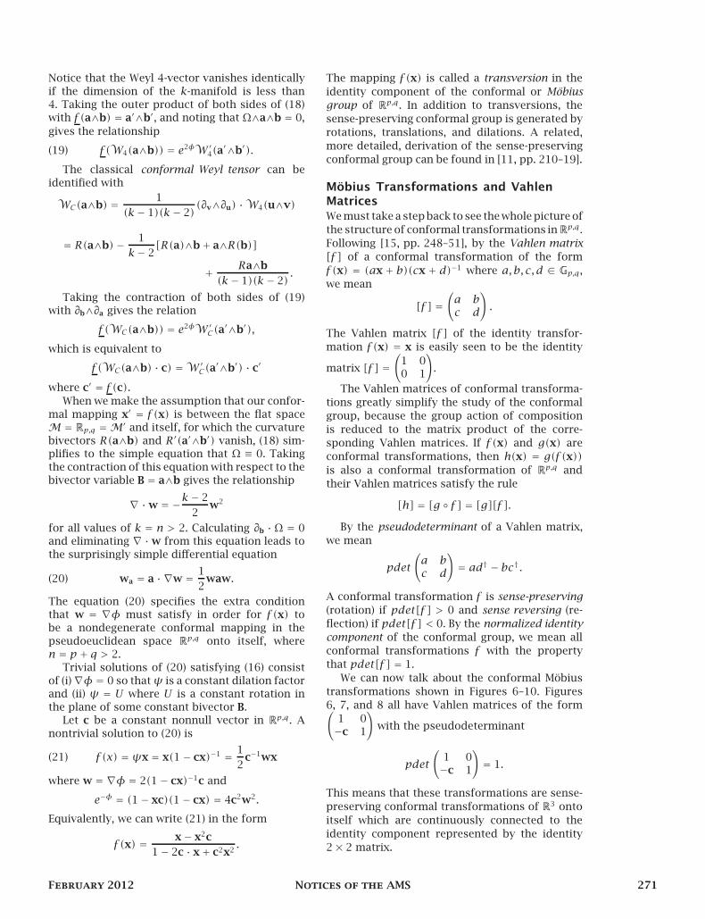
The mapping f (x) is called a transversion in the

identity component of the conformal or Möbius

group of Rp,q . In addition to transversions, the

sense-preserving conformal group is generated by

rotations, translations, and dilations. A related,

more detailed, derivation of the sense-preserving

conformal group can be found in [11, pp. 210–19].

Möbius Transformations and VahlenMatrices

We must take a step back to see the whole picture of

the structure of conformal transformations inRp,q .

Following [15, pp. 248–51], by the Vahlen matrix

[f ] of a conformal transformation of the form

f (x) = (ax + b)(cx + d)−1 where a, b, c, d ∈ Gp,q ,we mean

[f ] =(a bc d

).

The Vahlen matrix [f ] of the identity transfor-

mation f (x) = x is easily seen to be the identity

matrix [f ] =(

1 00 1

).

The Vahlen matrices of conformal transforma-

tions greatly simplify the study of the conformal

group, because the group action of composition

is reduced to the matrix product of the corre-

sponding Vahlen matrices. If f (x) and g(x) are

conformal transformations, then h(x) = g(f (x))is also a conformal transformation of Rp,q and

their Vahlen matrices satisfy the rule

[h] = [g f ] = [g][f ].By the pseudodeterminant of a Vahlen matrix,

we mean

pdet

(a bc d

)= ad† − bc†.

A conformal transformation f is sense-preserving

(rotation) if pdet[f ] > 0 and sense reversing (re-

flection) if pdet[f ] < 0. By the normalized identity

component of the conformal group, we mean all

conformal transformations f with the property

that pdet[f ] = 1.

We can now talk about the conformal Möbius

transformations shown in Figures 6–10. Figures

6, 7, and 8 all have Vahlen matrices of the form(1 0−c 1

)with the pseudodeterminant

pdet

(1 0−c 1

)= 1.

This means that these transformations are sense-

preserving conformal transformations of R3 onto

itself which are continuously connected to the

identity component represented by the identity

2× 2 matrix.

February 2012 Notices of the AMS 271

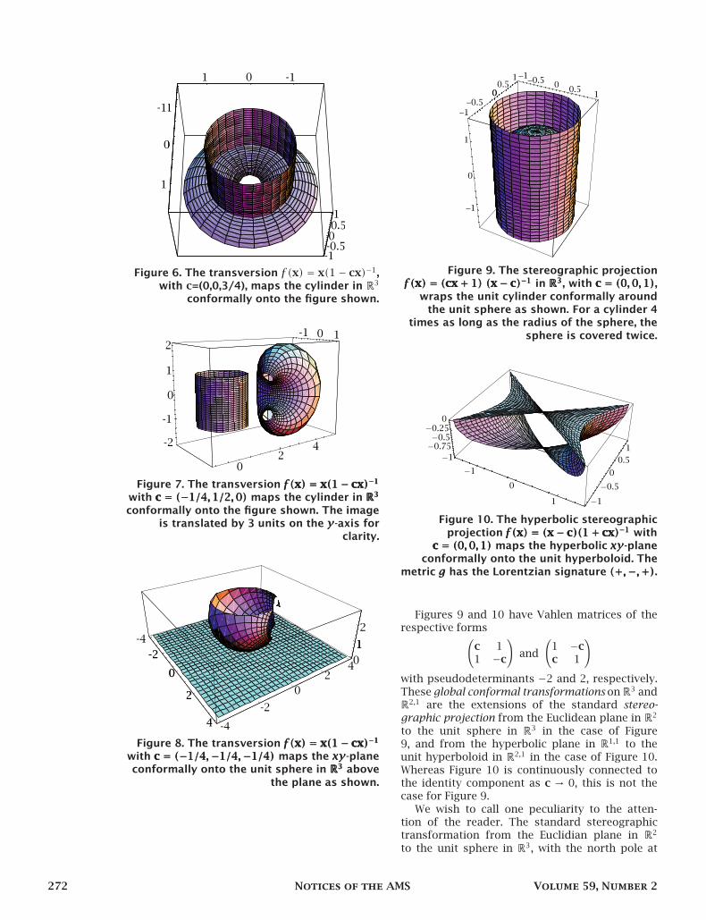
Figure 6. The transversion f (x) = x(1− cx)−1,with c=(0,0,3/4), maps the cylinder in R3

conformally onto the figure shown.

Figure 7. The transversion f (x) = x(1− cx)−1f (x) = x(1− cx)−1f (x) = x(1− cx)−1

with c = (−1/4,1/2, 0)c = (−1/4, 1/2,0)c = (−1/4, 1/2,0) maps the cylinder in R3R3R3

conformally onto the figure shown. The imageis translated by 3 units on the yyy-axis for

clarity.

Figure 8. The transversion f (x) = x(1− cx)−1f (x) = x(1− cx)−1f (x) = x(1− cx)−1

with c = (−1/4,−1/4,−1/4)c = (−1/4,−1/4,−1/4)c = (−1/4,−1/4,−1/4) maps the xyxyxy-planeconformally onto the unit sphere in R3R3R3 above

the plane as shown.

Figure 9. The stereographic projectionf (x) = (cx+ 1)f (x) = (cx+ 1)f (x) = (cx+ 1) (x− c)−1(x− c)−1(x− c)−1 in R3R3R3, with c = (0,0,1)c = (0,0,1)c = (0,0,1),

wraps the unit cylinder conformally aroundthe unit sphere as shown. For a cylinder 4

times as long as the radius of the sphere, thesphere is covered twice.

Figure 10. The hyperbolic stereographicprojection f (x) = (x− c)(1+ cx)−1f (x) = (x− c)(1+ cx)−1f (x) = (x− c)(1+ cx)−1 with

c = (0,0,1)c = (0,0,1)c = (0,0,1) maps the hyperbolic xyxyxy-planeconformally onto the unit hyperboloid. The

metric ggg has the Lorentzian signature (+,−,+)(+,−,+)(+,−,+).

Figures 9 and 10 have Vahlen matrices of therespective forms

(c 11 −c

)and

(1 −cc 1

)

with pseudodeterminants −2 and 2, respectively.These global conformal transformations onR3 andR2,1 are the extensions of the standard stereo-graphic projection from the Euclidean plane in R2

to the unit sphere in R3 in the case of Figure9, and from the hyperbolic plane in R1,1 to theunit hyperboloid in R2,1 in the case of Figure 10.Whereas Figure 10 is continuously connected tothe identity component as c → 0, this is not thecase for Figure 9.

We wish to call one peculiarity to the atten-tion of the reader. The standard stereographictransformation from the Euclidian plane in R2

to the unit sphere in R3, with the north pole at

272 Notices of the AMS Volume 59, Number 2

the unit vector e3 on the z-axis, can be repre-

sented either by f (x) = (e3x+ 1)(x − e3)−1 or by

g(x) = (x − e3)(e3x + 1)−1. Both of these trans-

formations are identical when restricted to the

xy-plane, but are globally distinct on R3. One of

these conformal transformations is sense preserv-

ing and continuously connected to the identity,

while the other one is not. How is this possible?

For the reader who wants to experiment with

these ideas but is not so familiar with geometricalgebra, I highly recommend the Clifford algebra

calculator software [16], which can be downloaded.

The reader may find it interesting to compare our

methods and results to those found in [8, pp.

106–118].

At the website http://www.garretstar.com/

algebra can be found supplementary material,

including the Links referred to in this article and

to other related websites, a discussion of the horo-sphere explaining the deep relationship between

the Vahlen matrices of elements in Gp,q to the

orthogonal group of Rp+1,q+1, and figures further

illustrating the richness of conformal mappings. At

present, the username: garretams and password:

garretams are required to view this material. Also

included is a list of additional references to the

literature to give the reader a better idea of the

many different applications that Clifford algebrashave found in mathematics, theoretical physics,

and in the computer science and engineering

communities.

AcknowledgmentsThe author wants to thank the reviewers of this

article for their helpful comments, which led to

improvements, and to the Universidad de Las

Américas-Puebla and to CONACYT SNI Exp. 14587

for their many years of support.

References[1] R. Ablamowicz and G. Sobczyk, Lectures on Clif-

ford (Geometric) Algebras and Applications, Birkhäuser,

Boston, 2004.

[2] H. Blaine Lawson and M. L. Michelson, Spin

Geometry, Princeton University Press, Princeton, 1989.

[3] F. Brackx, R. Delanghe, F. Sommen, Clifford Anal-

ysis, Pitman Publishers, Boston-London-Melbourne,

1982.

[4] C. J. S. Clarke, On the global isometric embedding

of pseudo-Riemannian manifolds, Proc. Roy. Soc. A 314,

417–428 (1970).

[5] T. Dantzig, NUMBER: The Language of Science,

Fourth Edition, Free Press, 1967.

[6] T. F. Havel, Geometric Algebra: Parallel Process-

ing for the Mind, Nuclear Engineering, 2002. See

Links 1.

[7] J. Gilbert and M. Murray, Clifford Algebras and

Dirac Operators in Harmonic Analysis, Cambridge

Studies in Advanced Mathematics, Cambridge Univer-

sity Press, Cambridge, 1991 (Online publication date:

November 2009).

[8] S. I. Goldberg, Curvature and Homology, Dover

Publications, New York, 1982.

[9] D. Hestenes, New Foundations for Classical Mechan-

ics, 2nd Ed., Kluwer, 1999.

[10] , Grassmann’s Legacy, in Grassmann Bi-

centennial Conference (1809–1877), September 16–19,

2009, Potsdam-Szczecin (DE, PL). See Links 2.

[11] D. Hestenes and G. Sobczyk, Clifford Alge-

bra to Geometric Calculus: A Unified Language for

Mathematics and Physics, 3rd edition, Kluwer, 1992.

[12] N. J. Hicks, Notes on Differential Geometry, Van

Nostrand, Princeton, NJ, 1965.

[13] D. Husemöller, Fibre Bundles, McGraw-Hill, New

York, 1966.

[14] J. M. Lee, Manifolds and Differential Geometry,

Graduate Studies in Mathematics, Vol. 107, American

Mathematical Society, Providence, RI, 2009.

[15] P. Lounesto, Clifford Algebras and Spinors, 2nd

edition, Cambridge University Press, Cambridge, 2001.

[16] , CLICAL Algebra Calculator and Software,

Helsinki University, 1987. See Links 3.

[17] C. W. Misner, K. S. Thorne and J. A. Wheeler,

Gravitation, Freeman and Company, San Francisco, CA,

1973.

[18] P. Nahin, An Imaginary Tale: The Story of the

Square Root of Minus One, Princeton University Press,

Princeton, NJ, 1998.

[19] J. Nash, C1 isometric imbeddings, Annals of

Mathematics (2), 60(3):383–396, 1954.

[20] , The imbedding problem for Riemannian

manifolds, Annals of Mathematics 2, 63(1):20–63, 1956.

[21] I. R. Porteous, Clifford Algebras and the Classical

Groups, Cambridge University Press, Cambridge, 1995.

[22] G. Sobczyk, Hyperbolic number plane, The College

Mathematics Journal, 26(4):269–280, September 1995.

[23] , Geometric matrix algebra, Linear Algebra

and its Applications, 429:1163–1173, 2008.

[24] , New Foundations in Mathematics: The Geo-

metric Concept of Number, San Luis Tehuiloyocan,

Mexico, 2010. See Links 4.

[25] , Plebanski classification of the tensor of

matter, Acta Physica Polonica, B11(6), 1981.

[26] , Mappings of Surfaces in Euclidean Space Us-

ing Geometric Algebra, Ph.D dissertation, Arizona State

University, 1971. See Links 5.

[27] J. Pozo and G. Sobczyk, Geometric algebra in linear

algebra and geometry, Acta Applicandae Mathematicae,

71: 207–244, 2002.

[28] M. Spivak, Calculus on Manifolds, W. A. Benjamin,

Inc., New York, 1965.

[29] D. J. Struik, A Concise History of Mathematics,

Dover, 1967.

[30] N. Verma, Towards an Algorithmic Realization of

Nash’s Embedding Theorem, CSE, UC San Diego. See

Links 6.

[31] E. Witten, Magic, mystery, and matrix, Notices

Amer. Math. Soc., 45(9):1124–1129, 1998.

[32] H. Whitney, Differentiable manifolds, Annals of

Mathematics (2), 37:645–680, 1936.

February 2012 Notices of the AMS 273