Public Choice99: 185–216, 1999.© 1999Kluwer Academic Publishers. Printed in the Netherlands.

185

Congressional distributive politics and state economicperformance∗

STEVEN D. LEVITT1 & JAMES M. POTERBA2

1University of Chicago and National Bureau of Economic Research;2MassachusettsInstitute of Technology and National Bureau of Economic Research

Accepted 26 March 1997

Abstract. States that were represented by very senior Democratic congressmen grew morequickly during the 1953–1990 period than states that were represented by more junior con-gressional delegations. States with a large fraction of politically competitive House districtsalso grew faster than average. The first finding is consistent with traditional legislator-basedmodels of distributive politics, the second with partisan models. We cannot detect any substan-tively important association between seniority, state political competition, and the geographicdistribution of federal funds, so higher district-specific federal spending does not appear to bethe source of the link between state economic growth and congressional representation.

When Senator Henry “Scoop” Jackson, the ranking Democrat on the SenateArmed Services Committee, died unexpectedly in September 1983, Roberts(1990) reports, the stock market values of defense contractors based in hishome state of Washington declined. The share prices of contractors based inGeorgia, the home state of the next-most-senior Democratic Senator on thecommittee, Sam Nunn, increased. When Senator George Mitchell of Maineannounced his plan to retire from the Senate at the end of his current term, theNew York Timesreported that “the most agonizing part of his decision. . . wasrecognizing that his position enabled him to help his home state in ways thata freshman taking his place could not” (March 6, 1994, p. 11).

A vast empirical literature has examined the link between Congressionalrepresentation and the distribution of government-controlled economic ben-efits. Anecdotal evidence suggests that districts represented by some seniorcongressmen have received disproportionate shares of some types of federalspending. Pearson and Anderson (1968) provide a particularly compellingaccount of former congressman Mendel Rivers (“Rivers Delivers”), chair ofthe House Armed Services Committee, and his efforts to channel military

∗ We are grateful to Julie Berry Cullen for outstanding research assistance, to Steve An-solabehere, Mark Crain, Alan Gerber, John Lott, Jeff Milyo, Sam Peltzman, Kim Rueben,Andrei Shleifer, James Snyder, Charles Stewart, seminar participants at Chicago, Harvard, theNBER, and Stanford, three anonymous referees, and especially to Keith Krehbiel and BarryWeingast for helpful discussions, and to the Center for Advanced Study in Behavioral Sciencesand National Science Foundation for research support.

186

spending to his district. Yet systematic empirical studies of committee mem-bership, congressional seniority and representation, and the distribution ofspending, including Atlas et al. (1995), Crain and Tollison (1977, 1981), Goss(1972), Greene and Munley (1980), Kiel and McKenzie (1983), Ray (1980,1981), Ritt (1976), Rundquist (1978), and Rundquist and Griffiths (1976),yield weak evidence on the link between representation and expenditures.

This paper re-examines the effect of congressional representation on thedistribution of economic benefits from federal government actions. It dif-fers from earlier empirical studies of distributive politics in two importantways. First, we analyze the effects of representation on an economicout-come, state per capita income growth, as well as on the geographic allocationof federal spending. Our approach recognizes the possibility that legislatorsaffect constituent welfare in many ways besides the direct allocation of fed-eral spending, for example by promoting regulatory and tax policies that arefavorable to district interests.

Second, we develop empirical tests of recent theories, such as those de-veloped by Kiewiet and McCubbins (1991) and Cox and McCubbins (1993),that highlight the role of congressional political parties as well as individuallegislator interests in affecting distributive politics. Partisan models of leg-islative behavior suggest that the self-interest of legislators may be served byfurthering the party’s fortunes, even if that comes at some expense to theirown district. This may require channelling resources to districts where themajority party holds a thin electoral majority so as to preserve the party’smajority status. To test these models, we identify politically competitive dis-tricts and compare their economic performance with that of “safe” one-partydistricts.

Our results provide support for both non-partisan and partisan models ofcongressional distributive politics. States with a higher fraction of very seniorDemocratic members of the House of Representatives experience faster percapita income growth than states with less senior delegations, although wefind no evidence of parallel effects for senior Senators. States with memberson particularly influential House committees experience more rapid growththan other states. We also find that states in which the two major political par-ties are competitive, measured either based on congressional or presidentialvote shares, also grow faster than less competitive states. These effects arenot simply an artifact of one group of states growing faster than another; theyare robust to our allowance for state-specific growth rates in our regressionmodels. In spite of these effects of political variables on economic growthrates, we find no consistent association between political variables and theallocation of federal spending, leaving us without a convincing explanationof the correlation between political variables and economic growth.

187

The paper is organized as follows. The first section summarizes the mod-els of congressional distributive politics that we attempt to test. Section twodescribes the data that form the basis for our analysis of congressional dele-gation composition, state political competitiveness, and economic growth inthe 1953–1990 period. The third section presents our empirical results. Thefourth section explores potential interpretations of these findings, focusingon whether seniority is a plausible cause of differential state growth rates,or whether causality is likely to run from economic growth to delegationseniority. Section five tests the hypothesis that seniority, committee mem-bership, and the degree of political competition affect state growth throughthe geographic distribution of federal spending. Section six concludes.

1. Distributive politics and congressional institutions

Formulating and testing models of Congressional institutions and their ef-fects on the geographical distribution of benefits from government programshas been an active subject of research in positive political economy duringthe last two decades. There are two broad categories of distributive models:nonpartisan models that emphasize incentives of individual legislators, andpartisan models that focus on the incentives of congressional political parties.Shepsle and Weingast (1994) survey much of the work in both categories.

Nonpartisan distributive politics models maintain that legislators attemptto maximize their chances of re-election by maximizing the policy benefitsaccruing to their constituents. While recognizing that legislators have dif-ferent amounts of influence over federal policies as a result of committeeposition and seniority rank, these models typically do not try to explain theorigins of such differential influence. These models have spawned a sub-stantial empirical literature studying geographic patterns in federal spend-ing, in particular the effect of congressional committee assignments on thesepatterns.

These empirical studies suffer from two key limitations. First, represen-tatives from districts with particular interests will be attracted to committeeswith control over policies that affect these interests. Farm state legislators arelikely to serve on the Agriculture Committee, and their districts are likelyto receive above-average levels farm support spending. This does not nec-essarily show that committee membership affects the allocation of spending.Second, the complex institutional structure of Congress, and the possibility oflog-rolling and other types of coalition formation, make it difficult to identifyinfluential members based solely on committee assignments.

Nonpartisan distributive politics models also have a conceptual limitation.They typically fail to explain how small legislative majorities can pursue pro-grams that benefit their constituents at the expense of others. Weingast (1979)

188

formalized a model of “universalism” to explain how legislation with highlylocalized benefits might pass with near-unanimity. He identified conditionsunder which it would be in the rational self-interest of all legislators to par-ticipate in a unanimous coalition, rather than in a smaller majority coalitionwith more narrowly distributed benefits. Recent work, notably Baron (1991),has questioned the theoretical presumption that universal coalitions shouldemerge in legislatures and shown that particular structures of agenda controlare likely to result in majoritarian rather than universalistic coalitions.1

Building on previous studies, we test two versions of the nonpartisandistributive politics model. One predicts that more senior legislators shouldbe able to channel greater economic benefits to their constituents, while thesecond predicts that influential committee members, and not senior membersper se, should capture benefits for their constituents. The two variants differbecause the seniority hypothesis allows senior members to achieve favorablepolicy outcomes even if they do not serve on the committee with jurisdic-tion over a given program, as a result of bargaining as described in Fiorina(1981).2

Partisan distributive politics models, developed for example by Coker andCrain (1994), Cox and McCubbins (1993), Rohde (1991), and Snyder (1994),have called attention to the potential importance of political parties, ratherthan individual legislators, as key decision makers. A party’s influence onpolicy rises discontinuously when it wins a majority in a legislative chamber.This can affect the career prospects of individual party members, who aremore likely to win re-election if their party has greater control over policy out-comes. If legislators in a party are concerned with obtaining a legislative ma-jority, and if resources (including the allocation of benefits from governmentprograms) have a higher effect on the expected number of party memberselected when they are allocated to highly-competitive political jurisdictionsrather than “safe” districts, then legislators may vote to allocate resources tocompetitive districts.3 Partisan distributive politics models therefore predict adifferent allocation of economic rewards than nonpartisan models.

2. Empirical framework and data construction

We explore the correlations between state economic growth, congressionaldelegation seniority, committee membership, and political competition. Tomotivate our analysis, assume that Y0

jt denotes per capita personal income injurisdiction j in year t in the absence of any economic effects of governmentactivity. Let Bjt denote the per capita benefits of government activities, andmodel Bjt = Xjt∗β, where Xjt is a vector of variables measuring legislatorinfluence. Bjt includes any effects on jurisdiction income associated with

189

federal spending in the district, as well as the effects of regulations or otherpolicies.4

Actual personal income is Yjt = Y0jt + Bjt.

One could test for the effect of legislator attributes on personal income byestimating regression models of the form

Yjt = Xjt ∗ β + Zjt ∗ γ + εjt. (2.1)

The variables in Zjt are controls for cross-sectional and time-series variationin the level of personal income absent government involvement, Y0

jt, suchas human capital, natural resources, and the physical capital stock. Becausethese factors are likely to be highly correlated over time and are difficult tomeasure, we assume that the lagged value of income in the jurisdiction, Yjt−1,can be used as a proxy for Zjt∗γ . We therefore write

Yjt − Yjt−1 = Xjt ∗ β + εjt. (2.2)

If personal income per capita is measured in logarithms, this specificationrelates the growth rate of personal income per capita to variables that measurelegislative influence. This equation forms the basis of our empirical work.5

Equation (2.2) implies that a state represented by a senior delegation growsmore quickly in every year during which that delegation is in office. This canbe contrasted with an alternative specification,1Yjt = 1Xjt∗β + κ jt , whichwould allow a one time increase in the income growth rate when the seniordelegation took office, and a one time drop when it left office, but no effectsin intervening periods. We have also investigated this alternative model, anddiscuss the results below.

We measure the growth rate of state real per capita personal income usingdata from the national income and product accounts, along with census dataon state population. We obtain similar results using disposable income, ratherthan personal income, in defining the dependent variable. The growth rate ofstate per capita personal income averaged 2.1% between 1949 and 1990, witha standard deviation computed across all states and years of 3.7%. States inthe South and the Northeast grew most quickly during this period, while statesin the Midwest and North Central regions grew slowest. States in the Southexperienced the most rapid growth early in the sample period, while those inthe Northeast grew quickly in the later years.

We focus on changes in state personal income, rather than congressionaldistrict income, for several reasons. First, data are reported more frequentlyon economic conditions at the state than at the district level. For congressionaldistricts, data are only available from the decennial census, and analyzingthese data is complicated by redistricting between census years.6 Second,

190

state data may be better for capturing “spillover” benefits from a powerful leg-islator that accrue to residents outside his district. Finally, testing distributivepolitics models in the Senate requires use of state-level data.

We measure congressional delegation seniority using a semi-parametricestimation approach that imposes minimal restrictions on the relationship be-tween our seniority variables and economic growth. We assign each memberof the House (Senate) to one of eleven (seven) seniority categories. For theHouse, we define six categories for Democrats and five for Republicans sinceDemocrats outnumbered Republicans in the House by an average of 81 overour sample period. Our categories correspond to the most senior 20 membersof each party, then the next 40, then those with seniority ranks 61 to 100,etc. We construct eleven summary statistics for each state’s congressionaldelegation seniority in each year, corresponding to the fraction of the state’srepresentatives in each category.7

We follow an analogous procedure for the Senate with four Democraticand three Republican categories.

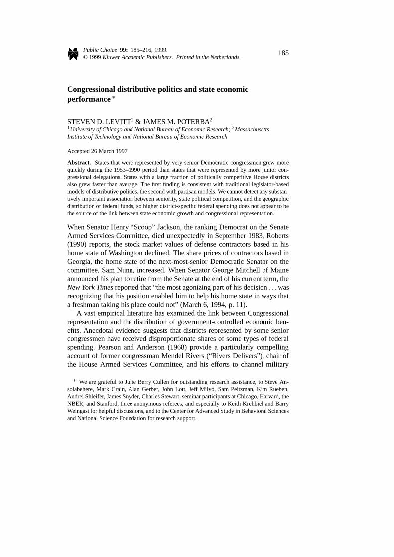
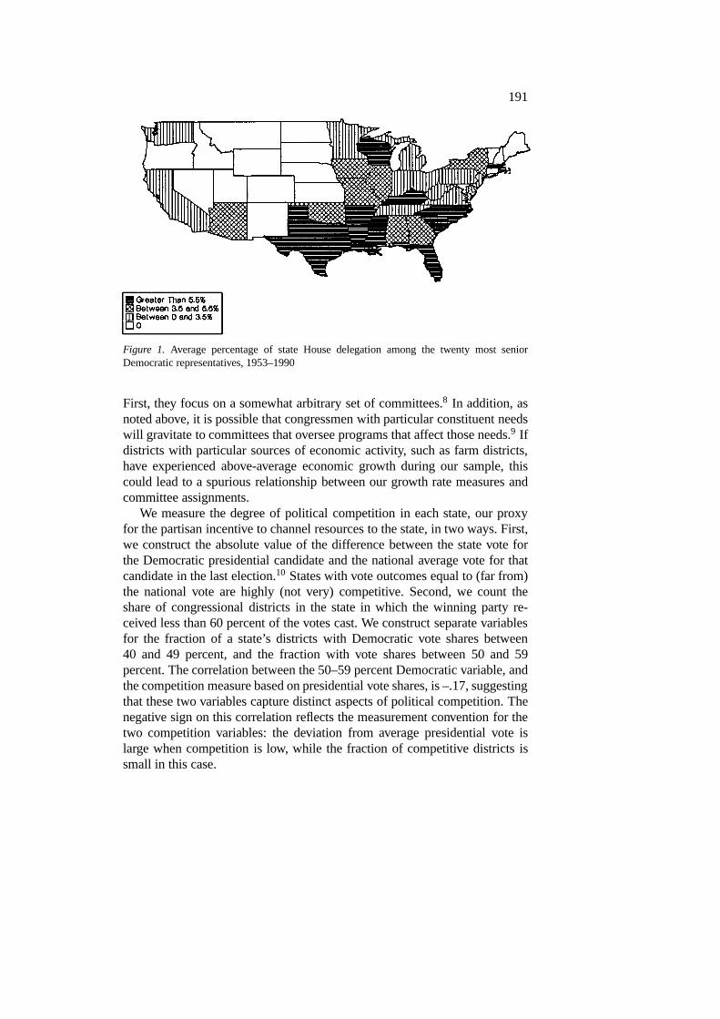
Figure 1 shows the average distribution of the 20 most senior House De-mocrats across state congressional delegations. The states with the highestaverage seniority concentrated in the South. Mississippi’s delegation is themost senior on average, with over one quarter of its members in the mostsenior twenty. The next highest state, Texas, averages 17% of its congressmenin the top 20. The disparities between Southern and other states were mostdramatic early in our sample period. Six states, Alabama, Arkansas, Georgia,Louisiana, Mississippi, and Texas, held 38% of the top 20 positions in thefirst half of our sample, compared with 22% in the second half.

The average growth rate of state per capita income over the 1953–1990period is strongly positively correlated with the average fraction of the state’sHouse delegation among the twenty most senior Democrats (ρ = .42). Whilesuggestive, this correlation isnot the basis for our subsequent empirical find-ings. We include state effects in most of our estimating equations, and there-fore identify the relationship between seniority and growth solely usingovertime, within statevariation in seniority.

We construct measures of committee-based influence by computing thefraction of delegation members on each of five particularly influential Housecommittees: Agriculture, Appropriations, Armed Services, Public Works, andWays and Means. We also calculate the fraction of the delegation memberswho are chairs or ranking minority members on these five committees. Thecorrelation between DEM 1–20 and committee chairs is .59; that betweenDEM 1–20 and membership on the key committees is .30.

Unlike our nonparametric seniority measures, our measures of committeeinfluence suffer from two limitations that have also plagued previous studies.

191

Figure 1. Average percentage of state House delegation among the twenty most seniorDemocratic representatives, 1953–1990

First, they focus on a somewhat arbitrary set of committees.8 In addition, asnoted above, it is possible that congressmen with particular constituent needswill gravitate to committees that oversee programs that affect those needs.9 Ifdistricts with particular sources of economic activity, such as farm districts,have experienced above-average economic growth during our sample, thiscould lead to a spurious relationship between our growth rate measures andcommittee assignments.

We measure the degree of political competition in each state, our proxyfor the partisan incentive to channel resources to the state, in two ways. First,we construct the absolute value of the difference between the state vote forthe Democratic presidential candidate and the national average vote for thatcandidate in the last election.10 States with vote outcomes equal to (far from)the national vote are highly (not very) competitive. Second, we count theshare of congressional districts in the state in which the winning party re-ceived less than 60 percent of the votes cast. We construct separate variablesfor the fraction of a state’s districts with Democratic vote shares between40 and 49 percent, and the fraction with vote shares between 50 and 59percent. The correlation between the 50–59 percent Democratic variable, andthe competition measure based on presidential vote shares, is –.17, suggestingthat these two variables capture distinct aspects of political competition. Thenegative sign on this correlation reflects the measurement convention for thetwo competition variables: the deviation from average presidential vote islarge when competition is low, while the fraction of competitive districts issmall in this case.

192

3. Distributive politics and state economic growth rates

Our basic regression model relates the growth rate in per capita personalincome in state i in year t (1 ln Yit) to a set of state and time effects as wellas variables for congressional delegation seniority, congressional committeeinfluence, and state political competition:

1lnYit = δi + ηt + β ∗ lnYi,t−1+6jαj ∗ SENIORITYjit

+6jγj ∗COMMITTEEjit +6jθj ∗COMPETITIONjit + εit.(3.1)

The year effects (ηt) capture the national business cycle, and contribute to therelatively high explanatory power of the reported equations. We frequentlyinclude the lagged value of state per capita income, following the recent “con-vergence” literature summarized in Barro and Sala-i-Martin (1995). Becauseyear-to-year variation in real income growth differs dramatically across states(the variance of North Dakota’s annual growth rate is 25 times greater thanNew York’s), we use a feasible generalized least squares procedure allowingfor heteroscedasticity of the form V(ε it ) = σ i

2. We limit our sample to the 48continental states.

3.1. Full sample results

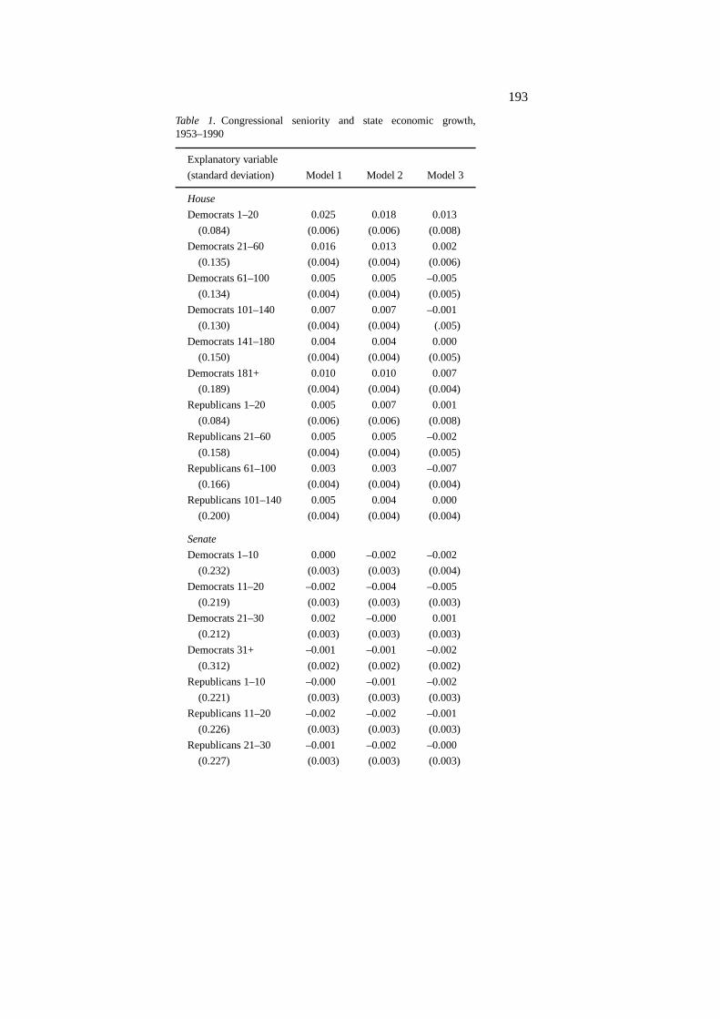
We first study the relationship between income growth and seniority, and thenwe introduce measures of committee membership and state political competi-tion. Table 1 reports estimates of equation (3.1), excluding the COMMITTEEand COMPETITION variables. The estimating equation in the first columnexcludes the lagged state income term and state fixed effects. The secondcolumn includes lagged state income, while the third column includes boththe lagged income variable and state fixed effects.

The coefficient estimates in the first column show that states with a highershare of very senior Democratic congressmen grew faster during our samplethan other states. The difference between the growth rate of a state withonly top 20 Democrats in its delegation, and a state with a House delega-tion that is comprised entirely of Republicans with seniority below 140 (the“excluded group” in our regression specification), is 2.5% per year. Shiftingone representative in a delegation of ten from the junior Republican to thesenior Democrat group, slightly more than a one standard deviation changein the DEM 1-20 variable, would be correlated with a 0.25 percentage pointincrease in the state’s income growth rate. The estimated effect of representa-tion by senior Democrats is attenuated, but remains statistically significantlydifferent from zero, when we include lagged state income in the growth ratespecification (column 2).11

193

Table 1. Congressional seniority and state economic growth,1953–1990

Explanatory variable

(standard deviation) Model 1 Model 2 Model 3

House

Democrats 1–20 0.025 0.018 0.013

(0.084) (0.006) (0.006) (0.008)

Democrats 21–60 0.016 0.013 0.002

(0.135) (0.004) (0.004) (0.006)

Democrats 61–100 0.005 0.005 –0.005

(0.134) (0.004) (0.004) (0.005)

Democrats 101–140 0.007 0.007 –0.001

(0.130) (0.004) (0.004) (.005)

Democrats 141–180 0.004 0.004 0.000

(0.150) (0.004) (0.004) (0.005)

Democrats 181+ 0.010 0.010 0.007

(0.189) (0.004) (0.004) (0.004)

Republicans 1–20 0.005 0.007 0.001

(0.084) (0.006) (0.006) (0.008)

Republicans 21–60 0.005 0.005 –0.002

(0.158) (0.004) (0.004) (0.005)

Republicans 61–100 0.003 0.003 –0.007

(0.166) (0.004) (0.004) (0.004)

Republicans 101–140 0.005 0.004 0.000

(0.200) (0.004) (0.004) (0.004)

Senate

Democrats 1–10 0.000 –0.002 –0.002

(0.232) (0.003) (0.003) (0.004)

Democrats 11–20 –0.002 –0.004 –0.005

(0.219) (0.003) (0.003) (0.003)

Democrats 21–30 0.002 –0.000 0.001

(0.212) (0.003) (0.003) (0.003)

Democrats 31+ –0.001 –0.001 –0.002

(0.312) (0.002) (0.002) (0.002)

Republicans 1–10 –0.000 –0.001 –0.002

(0.221) (0.003) (0.003) (0.003)

Republicans 11–20 –0.002 –0.002 –0.001

(0.226) (0.003) (0.003) (0.003)

Republicans 21–30 –0.001 –0.002 –0.000

(0.227) (0.003) (0.003) (0.003)

194

Table 1. continued.

Explanatory variable

(standard deviation) Model 1 Model 2 Model 3

ln Yi,t−1 0.017 –0.069

(0.003) (0.009)

State effects? No No Yes

F-test: House Democrats <.01 <.05 <.05

F-test: House Republicans >.65 >.50 >.45

F-test: Senate >.95 >.95 >.70

R2 0.572 0.585 0.576

Notes: Estimates are based on data for 48 states, 1953–1990, N = 1824.All specifications include exhaustive year effects (so no constant term) andare estimated by a feasible GLS procedure described in the text. Standarderrors are shown in parentheses. The standard deviation is the average ofthe annual standard deviations for the seniority variables. F-test values aresignificance bounds.

The results from estimating equations that do not include state fixed effectsare subject to a spurious “South effect.” During our sample period, Southernstates were on average represented by more senior delegations in Congress,and these states grew faster than the nation as a whole, possibly for reasonsunrelated to distributive politics. By allowing separate intercept terms foreach state (Table 1, column 3), we control for the possibility that some stateshave faster-than-average growth rates during this period, and thus identify thecoefficients only fromwithin state, over timevariation.12 The point estimateof the effect of very senior Democrats on state personal income growth issmaller when state effects are included than when they are not, but it remainspositive and marginally statistically significant.13

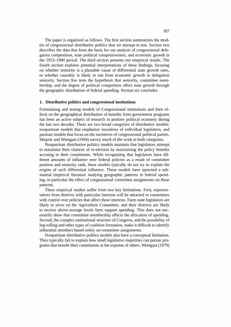
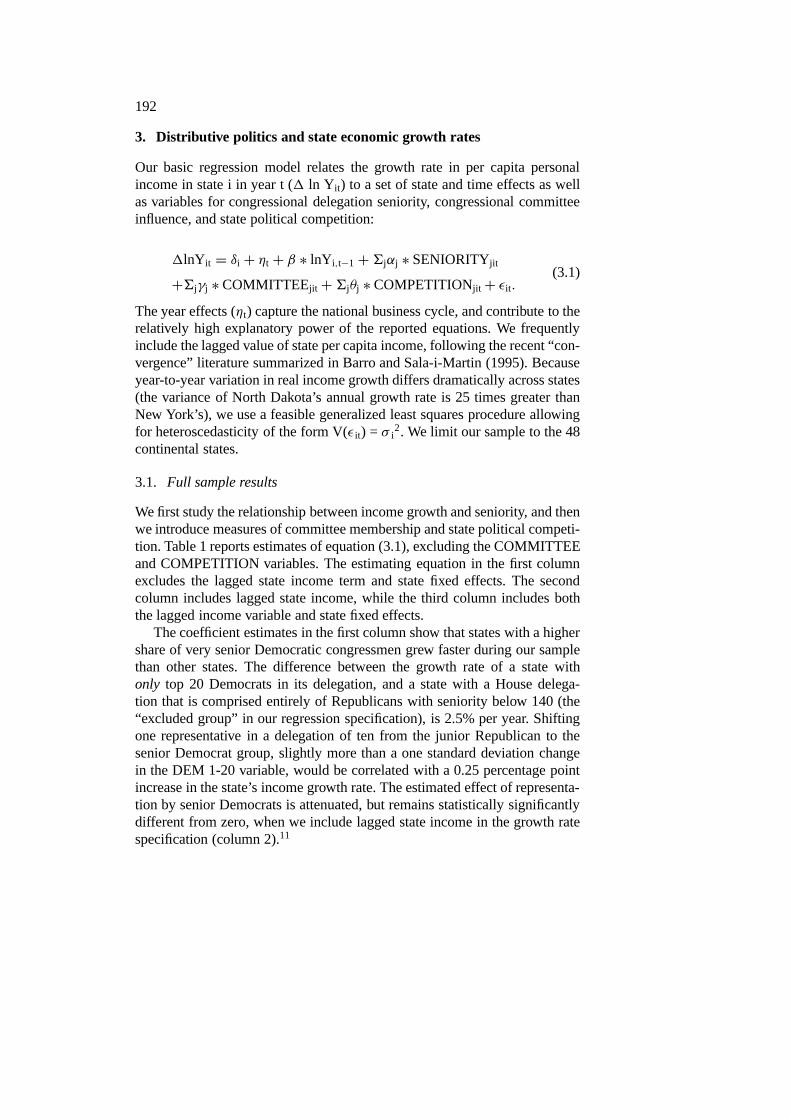
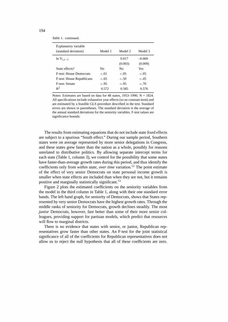
Figure 2 plots the estimated coefficients on the seniority variables fromthe model in the third column in Table 1, along with their one standard errorbands. The left hand graph, for seniority of Democrats, shows that States rep-resented by very senior Democrats have the highest growth rates. Through themiddle ranks of seniority for Democrats, growth declines steadily. The mostjunior Democrats, however, fare better than some of their more senior col-leagues, providing support for partisan models, which predict that resourceswill flow to marginal districts.

There is no evidence that states with senior, or junior, Republican rep-resentatives grow faster than other states. An F-test for the joint statisticalsignificance of all of the coefficients for Republican representatives does notallow us to reject the null hypothesis that all of these coefficients are zero.

195

Figure 2. Effect of congressional seniority variables on state economic growth: Point estimateand one standard error bands

Similarly, we cannot reject the hypothesis that all of the coefficients on theSenate seniority variables are jointly zero. We also explored interaction vari-ables that identified states with very senior House and Senate delegations;we found no effect beyond that of the House variables. We therefore limitour set of SENIORITY variables to those for House Democrats when weadd COMMITTEE and COMPETITION variables; including the full set ofseniority variables does not change the results.

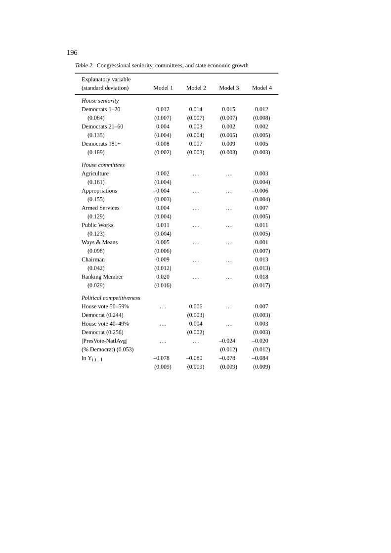
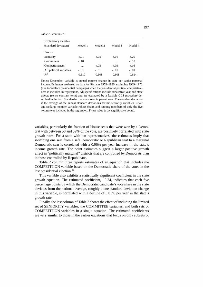
Table 2 reports the results of adding the COMMITTEE and COMPE-TITION variables to the basic specification. The equation in column oneprovides mixed evidence of committee effects. The null hypothesis that allcommittee variables have zero coefficients can be rejected at the .10, butnot the .05, confidence level. Public Works is the only committee member-ship that exhibits a strong positive correlation with personal income growth.The estimated coefficient, .011, implies that switching one House member’scommittee assignment from a non-influential committee to Public Works ina ten-member delegation will lead to an increase of 0.1% in annual stateeconomic growth. This finding is consistent with Ferejohn’s (1974) resultthat there is some geographical bias in public infrastructure spending towardthe districts of Public Works committee members.

Table 2 column two includes the reduced set of SENIORITY variablesas well as the two variables that measure a state’s political competitivenesson the basis of its share of close-contest House seats. The COMPETITION

196

Table 2. Congressional seniority, committees, and state economic growth

Explanatory variable

(standard deviation) Model 1 Model 2 Model 3 Model 4

House seniority

Democrats 1–20 0.012 0.014 0.015 0.012

(0.084) (0.007) (0.007) (0.007) (0.008)

Democrats 21–60 0.004 0.003 0.002 0.002

(0.135) (0.004) (0.004) (0.005) (0.005)

Democrats 181+ 0.008 0.007 0.009 0.005

(0.189) (0.002) (0.003) (0.003) (0.003)

House committees

Agriculture 0.002 . . . . . . 0.003

(0.161) (0.004) (0.004)

Appropriations –0.004 . . . . . . –0.006

(0.155) (0.003) (0.004)

Armed Services 0.004 . . . . . . 0.007

(0.129) (0.004) (0.005)

Public Works 0.011 . . . . . . 0.011

(0.123) (0.004) (0.005)

Ways & Means 0.005 . . . . . . 0.001

(0.098) (0.006) (0.007)

Chairman 0.009 . . . . . . 0.013

(0.042) (0.012) (0.013)

Ranking Member 0.020 . . . . . . 0.018

(0.029) (0.016) (0.017)

Political competitiveness

House vote 50–59% . . . 0.006 . . . 0.007

Democrat (0.244) (0.003) (0.003)

House vote 40–49% . . . 0.004 . . . 0.003

Democrat (0.256) (0.002) (0.003)

|PresVote-NatlAvg| . . . . . . –0.024 –0.020

(% Democrat) (0.053) (0.012) (0.012)

ln Yi,t−1 –0.078 –0.080 –0.078 –0.084

(0.009) (0.009) (0.009) (0.009)

197

Table 2. continued.

Explanatory variable

(standard deviation) Model 1 Model 2 Model 3 Model 4

F-tests:

Seniority <.01 <.05 <.01 <.20

Committees <.10 . . . . . . <.10

Competitiveness . . . <.05 <.05 <.05

All political variables <.01 <.01 <.01 <.01

R2 0.610 0.608 0.608 0.614

Notes: Dependent variable is annual percent change in state per capita personalincome. Estimates are based on data for 48 states 1953–1990, excluding 1969–1972(due to Wallace presidential campaign) when the presidential political competitive-ness is included in regressions. All specifications include exhaustive year and stateeffects (so no constant term) and are estimated by a feasible GLS procedure de-scribed in the text. Standard errors are shown in parentheses. The standard deviationis the average of the annual standard deviations for the seniority variables. Chairand ranking member variable reflect chairs and ranking members of only the fivecommittees included in the regression. F-test value is the significance bound.

variables, particularly the fraction of House seats that were won by a Demo-crat with between 50 and 59% of the vote, are positively correlated with stategrowth rates. For a state with ten representatives, the estimates imply thatswitching one seat from a safe Democratic or Republican seat to a marginalDemocratic seat is correlated with a 0.06% per year increase in the state’sincome growth rate. The point estimates suggest a larger positive growtheffect in “politically marginal” districts that are controlled by Democrats thanin those controlled by Republicans.

Table 2 column three reports estimates of an equation that includes theCOMPETITION variable based on the Democratic share of the votes in thelast presidential election.14

This variable also exhibits a statistically significant coefficient in the stategrowth equation. The estimated coefficient, –0.24, indicates that each fivepercentage points by which the Democratic candidate’s vote share in the statedeviates from the national average, roughly a one standard deviation changein this variable, is correlated with a decline of 0.01% per year in the state’sgrowth rate.

Finally, the last column of Table 2 shows the effect of including the limitedset of SENIORITY variables, the COMMITTEE variables, and both sets ofCOMPETITION variables in a single equation. The estimated coefficientsare very similar to those in the earlier equations that focus on only subsets of

198

these variables. Including the COMPETITION and COMMITTEE variableshas very little effect on the estimated SENIORITY effects.

To explore the robustness of our findings, we also estimate several regres-sion models relating per capita personal income growth to other summarystatistics on delegation structure. Including two indicator variables, set equalto one for states represented by the chairs or ranking minority members on ourfive key committees, in a specification otherwise like that in the third columnof Table 1, yielded positive estimated growth effects. The point estimates(standard errors) are .017 (.011) and .017 (.016), respectively. We also triedincluding the percent of the state’s House delegation that is Democratic; thisvariable has a substantial positive effect, with a coefficient of .0044 (.0022).The fraction of Democratic senators in the state delegation had a near-zero,and statistically insignificantly different from zero, effect on state growth. Thepercent of the state’s House delegates on the five key committees we considerhas a positive but statistically insignificant effect on state growth (coefficientof .0022, standard error .0021). These results generally support the findings inour preferred specifications, and suggest that there is an association betweenthe structure of representation and economic growth rates.

3.2. Caveats and objections

One potential objection to our analysis concerns our focus on per capita ratherthan total income growth. If individuals can migrate costlessly in responseto income differentials, then any policy that raises a jurisdiction’s total in-come would lead to immigration, with no net effect on per capita income.Our coefficients might therefore under-estimate the effect of congressionalrepresentation on income growth.

Two factors lead us to doubt this interpretation. First, available evidenceon migration elasticities, such as that presented in Blanchard and Katz (1992),suggests that income differentials are equilibrated by migration over a periodof between five and fifteen years. In contrast, we are considering immediateeffects of representation on economic growth. Second, we have estimated theregression equations in Table 2 with total rather than per capita income asthe dependent variable. The point estimates on the SENIORITY and COM-PETITION variables are smaller in this case, while the coefficients on theAgriculture, Armed Services, and Public Works committees are larger andmore statistically significant than in the per capita income equations. Theseresults do not correspond to the pattern one would expect in the case ofsystematic bias.

A second potential objection, and an issue we noted above, concerns ourmodelling growth rates as a function of the level of delegation variables,rather than theirchanges. We estimated, but do not report, models in which

199

current as well as lagged seniority and similar variables are included in theregression model; this specification is an unrestricted form of the differencemodel. These results suggest that the greatest effect of seniority on growthoccurs when a congressman first becomes senior, and that a state thatwas, butis no longer, represented by a senior delegation grows slower than the averagestate. The net effect of a senior delegation, adding together both current andfuture growth rate effects, is similar to that in our equations with only thelevel of seniority and other delegation variables.

3.3. Subsample results

Congress has evolved during our sample period in ways that could alter thelink between congressional representation and growth. First, relative partystrengths in the Congress have varied. There was relative balance betweenthe parties early in our sample, but the Democratic party held a comfortablemajority in the House for most of the second half of our sample. Our sampleends in 1990, well before the shift to Republican control in the House thatoccurred in November 1994. Second, civil rights, a divisive issue within theDemocratic party, became less important in the latter half of our sample,leading to increased concentration of power in the hands of Democrats vis-a-vis Republicans as the sample evolves. Third, as Reiselbach (1986) describes,the congressional reforms of the early 1970s reduced the importance of com-mittee chairs, increased the influence of junior members, and shifted powertoward members of the Steering and Policy Committee. Finally, the federalgovernment’s growing economic role over the last four decades has expandedthe potential for political factors to affect state growth rates.

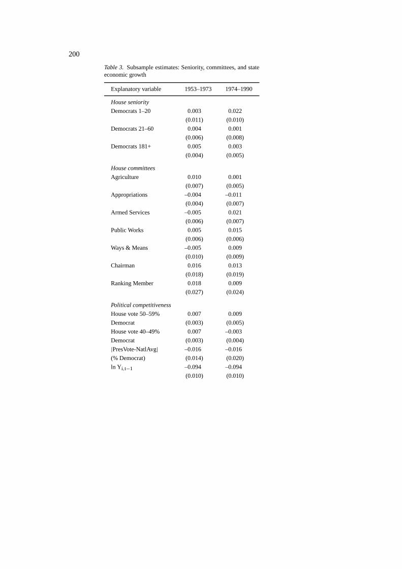
Table 3 tests sub-sample stability using the specification reported in Ta-ble 2 column four. The sample is divided in 1974, which coincides with sub-stantial Congressional reforms as well as the first OPEC oil shock. We allowthe coefficients on all of the political variables to differ between the first andsecond sample periods, but we constrain the coefficient on the lagged incomevariable, and the state effect coefficients, to be equal in the two periods.

The results in Table 3 suggest that states represented by senior Democraticdelegations enjoyed faster-than-average economic growth in both sample pe-riods, but especially in the periodsince1974. This result is consistent withincreased Democratic control of the House and growth in the scope of govern-ment, but surprising in light of the congressional reforms.15 With respect tocommittee membership, there are several changes across sub-samples. Mem-bership on the House Agriculture Committee was more strongly correlatedwith state growth in the early than in the later part of the sample period,and the value of members on the House Public Works and Armed ServicesCommittees was larger for the post-1974 than earlier period. The coefficients

200

Table 3. Subsample estimates: Seniority, committees, and stateeconomic growth

Explanatory variable 1953–1973 1974–1990

House seniority

Democrats 1–20 0.003 0.022

(0.011) (0.010)

Democrats 21–60 0.004 0.001

(0.006) (0.008)

Democrats 181+ 0.005 0.003

(0.004) (0.005)

House committees

Agriculture 0.010 0.001

(0.007) (0.005)

Appropriations –0.004 –0.011

(0.004) (0.007)

Armed Services –0.005 0.021

(0.006) (0.007)

Public Works 0.005 0.015

(0.006) (0.006)

Ways & Means –0.005 0.009

(0.010) (0.009)

Chairman 0.016 0.013

(0.018) (0.019)

Ranking Member 0.018 0.009

(0.027) (0.024)

Political competitiveness

House vote 50–59% 0.007 0.009

Democrat (0.003) (0.005)

House vote 40–49% 0.007 –0.003

Democrat (0.003) (0.004)

|PresVote-NatlAvg| –0.016 –0.016

(% Democrat) (0.014) (0.020)

ln Yi,t−1 –0.094 –0.094

(0.010) (0.010)

201

Table 3. continued.

Explanatory variable 1953–1973 1974–1990

F-test: Sub-sample stability

Seniority . . . >.50

Committees . . . <.10

Competitiveness . . . <.25

All political variables . . . <.10

Notes: Dependent variable is annual percent change in state percapita personal income. Estimates are based on data for 48 states,excluding 1969–1972 (due to Wallace presidential campaign)when the presidential political competitiveness is included inregressions. Specification includes exhaustive year and stateeffects (so no constant term) and is estimated by a feasible GLSprocedure described in the text. State fixed-effects are constrainedto be constant across the two time periods. Standard errors areshown in parentheses. Chair and ranking member variable reflectchairs and ranking members of only the five committees includedin the regression. F-test value is the significance bound.

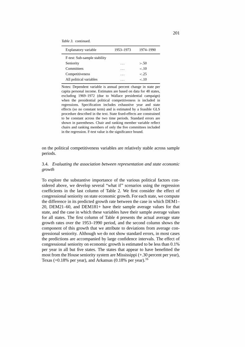
on the political competitiveness variables are relatively stable across sampleperiods.

3.4. Evaluating the association between representation and state economicgrowth

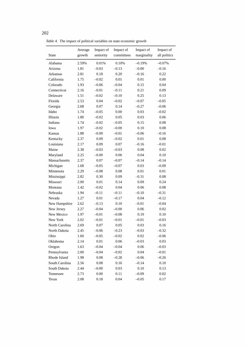
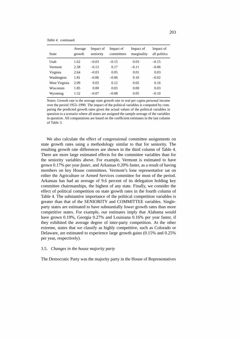
To explore the substantive importance of the various political factors con-sidered above, we develop several “what if” scenarios using the regressioncoefficients in the last column of Table 2. We first consider the effect ofcongressional seniority on state economic growth. For each state, we computethe difference in its predicted growth rate between the case in which DEM1–20, DEM21–60, and DEM181+ have their sample average values for thatstate, and the case in which these variables have their sample average valuesfor all states. The first column of Table 4 presents the actual average stategrowth rates over the 1953–1990 period, and the second column shows thecomponent of this growth that we attribute to deviations from average con-gressional seniority. Although we do not show standard errors, in most casesthe predictions are accompanied by large confidence intervals. The effect ofcongressional seniority on economic growth is estimated to be less than 0.1%per year in all but five states. The states that appear to have benefitted themost from the House seniority system are Mississippi (+.30 percent per year),Texas (+0.18% per year), and Arkansas (0.18% per year).16

202

Table 4. The impact of political variables on state economic growth

Average Impact of Impact of Impact of Impact of

State growth seniority committees marginality all politics

Alabama 2.59% 0.01% 0.10% –0.19% –0.07%

Arizona 1.81 –0.03 –0.13 –0.00 –0.16

Arkansas 2.81 0.18 0.20 –0.16 0.22

California 1.75 –0.02 0.01 0.01 0.00

Colorado 1.93 –0.06 –0.04 0.15 0.04

Connecticut 2.16 –0.01 –0.11 0.21 0.09

Delaware 1.51 –0.02 –0.10 0.25 0.13

Florida 2.53 0.04 –0.02 –0.07 –0.05

Georgia 2.68 0.07 0.14 –0.27 –0.06

Idaho 1.74 –0.05 0.00 0.03 –0.02

Illinois 1.80 –0.02 0.05 0.03 0.06

Indiana 1.74 –0.02 –0.05 0.15 0.08

Iowa 1.97 –0.02 –0.00 0.10 0.08

Kansas 1.88 –0.09 –0.01 –0.06 –0.16

Kentucky 2.37 0.09 –0.02 0.01 0.08

Louisiana 2.17 0.09 0.07 –0.16 –0.01

Maine 2.38 –0.03 –0.03 0.08 0.02

Maryland 2.25 –0.00 0.06 0.04 0.10

Massachusetts 2.37 0.07 –0.07 –0.14 –0.14

Michigan 1.68 –0.05 –0.07 0.03 –0.09

Minnesota 2.29 –0.08 0.08 0.01 0.01

Mississippi 2.82 0.30 0.09 –0.31 0.08

Missouri 2.00 0.01 0.14 0.09 0.24

Montana 1.42 –0.02 0.04 0.06 0.08

Nebraska 1.94 –0.11 –0.11 –0.10 –0.31

Nevada 1.27 0.01 –0.17 0.04 –0.12

New Hampshire 2.62 –0.13 0.10 –0.01 –0.04

New Jersey 2.27 –0.04 –0.00 0.06 0.02

New Mexico 1.97 –0.01 –0.08 0.19 0.10

New York 2.02 –0.01 –0.01 –0.01 –0.03

North Carolina 2.69 0.07 0.05 0.03 0.16

North Dakota 2.45 –0.06 –0.23 –0.03 –0.32

Ohio 1.60 –0.05 –0.02 0.02 –0.06

Oklahoma 2.14 0.01 0.06 –0.03 0.03

Oregon 1.63 –0.04 –0.04 0.06 –0.03

Pennsylvania 2.00 –0.04 –0.02 0.04 –0.01

Rhode Island 1.98 0.08 –0.28 –0.06 –0.26

South Carolina 2.56 0.08 0.16 –0.14 0.10

South Dakota 2.44 –0.00 0.03 0.10 0.13

Tennessee 2.73 0.00 0.11 –0.09 0.02

Texas 2.08 0.18 0.04 –0.05 0.17

203

Table 4. continued.

Average Impact of Impact of Impact of Impact of

State growth seniority committees marginality all politics

Utah 1.62 –0.03 –0.15 0.03 –0.15

Vermont 2.58 –0.13 0.17 –0.11 –0.06

Virginia 2.64 –0.03 0.05 0.01 0.03

Washington 1.81 –0.06 –0.06 0.10 –0.02

West Virginia 2.09 0.03 0.12 0.02 0.16

Wisconsin 1.85 0.00 0.03 0.00 0.03

Wyoming 1.52 –0.07 –0.08 0.05 –0.10

Notes: Growth rate is the average state growth rate in real per capita personal incomeover the period 1953–1990. The impact of the political variables is computed by com-paring the predicted growth rates given the actual values of the political variables inquestion to a scenario where all states are assigned the sample average of the variablesin question. All computations are based on the coefficient estimates in the last columnof Table 3.

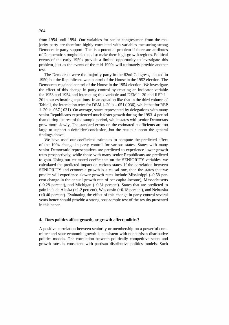
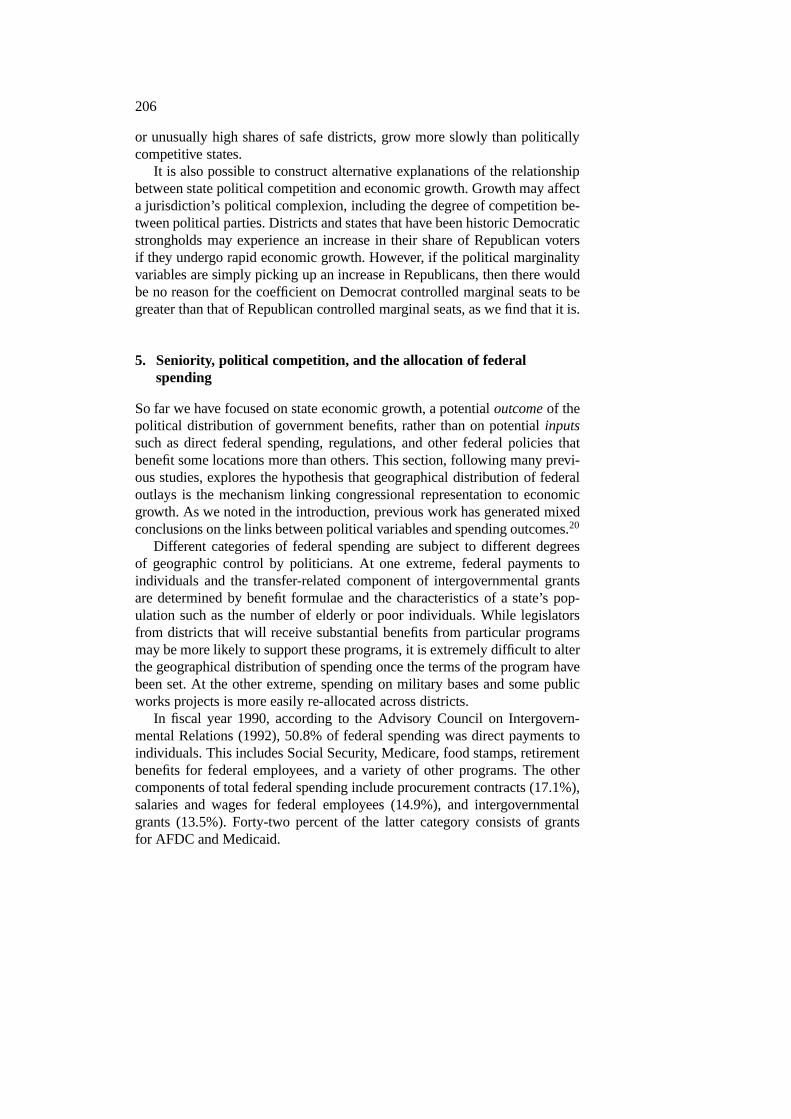
We also calculate the effect of congressional committee assignments onstate growth rates using a methodology similar to that for seniority. Theresulting growth rate differences are shown in the third column of Table 4.There are more large estimated effects for the committee variables than forthe seniority variables above. For example, Vermont is estimated to havegrown 0.17% per yearfaster, and Arkansas 0.20% faster, as a result of havingmembers on key House committees. Vermont’s lone representative sat oneither the Agriculture or Armed Services committee for most of the period.Arkansas has had an average of 9.6 percent of its delegation holding keycommittee chairmanships, the highest of any state. Finally, we consider theeffect of political competition on state growth rates in the fourth column ofTable 4. The substantive importance of the political competition variables isgreater than that of the SENIORITY and COMMITTEE variables. Single-party states are estimated to have substantially lower growth rates than morecompetitive states. For example, our estimates imply that Alabama wouldhave grown 0.19%, Georgia 0.27% and Louisiana 0.16% per year faster, ifthey exhibited the average degree of inter-party competition. At the otherextreme, states that we classify as highly competitive, such as Colorado orDelaware, are estimated to experience large growth gains (0.15% and 0.25%per year, respectively).

3.5. Changes in the house majority party

The Democratic Party was the majority party in the House of Representatives

204

from 1954 until 1994. Our variables for senior congressmen from the ma-jority party are therefore highly correlated with variables measuring strongDemocratic party support. This is a potential problem if there are attributesof Democratic strongholds that also make them high-growth regions. Politicalevents of the early 1950s provide a limited opportunity to investigate thisproblem, just as the events of the mid-1990s will ultimately provide anothertest.

The Democrats were the majority party in the 82nd Congress, elected in1950, but the Republicans won control of the House in the 1952 election. TheDemocrats regained control of the House in the 1954 election. We investigatethe effect of this change in party control by creating an indicator variablefor 1953 and 1954 and interacting this variable and DEM 1–20 and REP 1–20 in our estimating equations. In an equation like that in the third column ofTable 1, the interaction term for DEM 1–20 is –.051 (.036), while that for REP1–20 is .037 (.031). On average, states represented by delegations with manysenior Republicans experienced much faster growth during the 1953–4 periodthan during the rest of the sample period, while states with senior Democratsgrew more slowly. The standard errors on the estimated coefficients are toolarge to support a definitive conclusion, but the results support the generalfindings above.

We have used our coefficient estimates to compute the predicted effectof the 1994 change in party control for various states. States with manysenior Democratic representatives are predicted to experience lower growthrates prospectively, while those with many senior Republicans are predictedto gain. Using our estimated coefficients on the SENIORITY variables, wecalculated the predicted impact on various states. If the correlation betweenSENIORITY and economic growth is a causal one, then the states that wepredict will experience slower growth rates include Mississippi (–0.58 per-cent change in the annual growth rate of per capita income), Massachusetts(–0.28 percent), and Michigan (–0.31 percent). States that are predicted togain include Alaska (+1.2 percent), Wisconsin (+0.18 percent), and Nebraska(+0.40 percent). Evaluating the effect of this change in party control severalyears hence should provide a strong post-sample test of the results presentedin this paper.

4. Does politics affect growth, or growth affect politics?

A positive correlation between seniority or membership on a powerful com-mittee and state economic growth is consistent with nonpartisan distributivepolitics models. The correlation between politically competitive states andgrowth rates is consistent with partisan distributive politics models. Such

205

correlations do not uniquely support these models of congressional decision-making, however. In particular, there are several alternative explanations forthese findings that involve a “reverse causality” between economic growthand political variables. With respect to the association between legislatorseniority and economic growth, it is possible that voters in states that ex-perience more rapid economic growth are more likely to re-elect incumbentlegislators, thereby inducing a positive correlation between growth rates andseniority. If district economic performance wasnot related to the vote for theincumbent, it is hard to understand why elected officials would exert effortto affect their district economy.17 Yet this effect does not appear to explainour findings, which relate economic growth during the current year to theseniority of legislators who were elected one or two years ago.

The seniority of incumbents is, therefore, related to the past history ofeconomic growth in the district, not the current growth rate. If there is se-rial correlation in state economic growth rates, and we fail to control forlagged growth, our coefficients may nonetheless be biased.18 We can con-trol for such effects directly by including lagged values of the state growthrate in our equations. We illustrate the findings by reference to the equationin the fourth column of Table 2; other specifications confirm the results.Without lagged growth rate terms, the coefficients on DEM1–20, DEM21–60, and DEM181+ are .012 (.007), .002 (.005), and .005 (.003), respectively.Adding six lagged values of annual state economic growth to this specifica-tion changes the House Democratic seniority variables to .013 (.008), .002(.005), and .005 (.003), respectively. The lagged growth variables have sta-tistically significant effects in predicting the current growth rate, but addingthem to the model does not alter our estimated relationship between legisla-tive influence and current economic growth.19

Another potential explanation for the correlation between legislator se-niority and state growth is that states with more senior congressmen are morehomogeneous than states with more junior delegations. A solid majority fora single party in a congressional district is a prerequisite for continued re-election of the same congressman, hence for seniority. If homogeneity is goodfor growth, a spurious correlation between seniority and growth could arise.

There are three reasons to doubt this explanation of our results. First, ifhomogeneityper seis the source of growth, then the coefficient on seniorRepublicans should also be significantly positive, yet we find no evidencefor this. Second, our estimates that allow for state fixed effects in the rate ofeconomic growth should capture factors such as state homogeneity. Finally,this alternative hypothesis conflicts with our finding that states with extremevalues of either Democratic or Republican votes for presidential candidates,

206

or unusually high shares of safe districts, grow more slowly than politicallycompetitive states.

It is also possible to construct alternative explanations of the relationshipbetween state political competition and economic growth. Growth may affecta jurisdiction’s political complexion, including the degree of competition be-tween political parties. Districts and states that have been historic Democraticstrongholds may experience an increase in their share of Republican votersif they undergo rapid economic growth. However, if the political marginalityvariables are simply picking up an increase in Republicans, then there wouldbe no reason for the coefficient on Democrat controlled marginal seats to begreater than that of Republican controlled marginal seats, as we find that it is.

5. Seniority, political competition, and the allocation of federalspending

So far we have focused on state economic growth, a potentialoutcomeof thepolitical distribution of government benefits, rather than on potentialinputssuch as direct federal spending, regulations, and other federal policies thatbenefit some locations more than others. This section, following many previ-ous studies, explores the hypothesis that geographical distribution of federaloutlays is the mechanism linking congressional representation to economicgrowth. As we noted in the introduction, previous work has generated mixedconclusions on the links between political variables and spending outcomes.20

Different categories of federal spending are subject to different degreesof geographic control by politicians. At one extreme, federal payments toindividuals and the transfer-related component of intergovernmental grantsare determined by benefit formulae and the characteristics of a state’s pop-ulation such as the number of elderly or poor individuals. While legislatorsfrom districts that will receive substantial benefits from particular programsmay be more likely to support these programs, it is extremely difficult to alterthe geographical distribution of spending once the terms of the program havebeen set. At the other extreme, spending on military bases and some publicworks projects is more easily re-allocated across districts.

In fiscal year 1990, according to the Advisory Council on Intergovern-mental Relations (1992), 50.8% of federal spending was direct payments toindividuals. This includes Social Security, Medicare, food stamps, retirementbenefits for federal employees, and a variety of other programs. The othercomponents of total federal spending include procurement contracts (17.1%),salaries and wages for federal employees (14.9%), and intergovernmentalgrants (13.5%). Forty-two percent of the latter category consists of grantsfor AFDC and Medicaid.

207

Data on the state-by-state allocation of various components of federalspending are available for different sample periods. For direct payments toindividuals, federal wages and salaries, and intergovernmental grants, wehave data for the 1958–1990 period. Overall procurement spending data isonly available beginning in 1982, so we instead use Department of Defenseprime contract awards, which account for approximately 75 percent of overallprocurement, and for which data are available since 1959. We also considertotal federal outlays, but data for this aggregate are only available for the1970–1990 period, with data missing in 1971 and 1977.

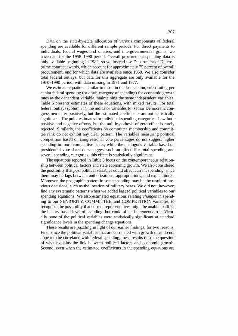
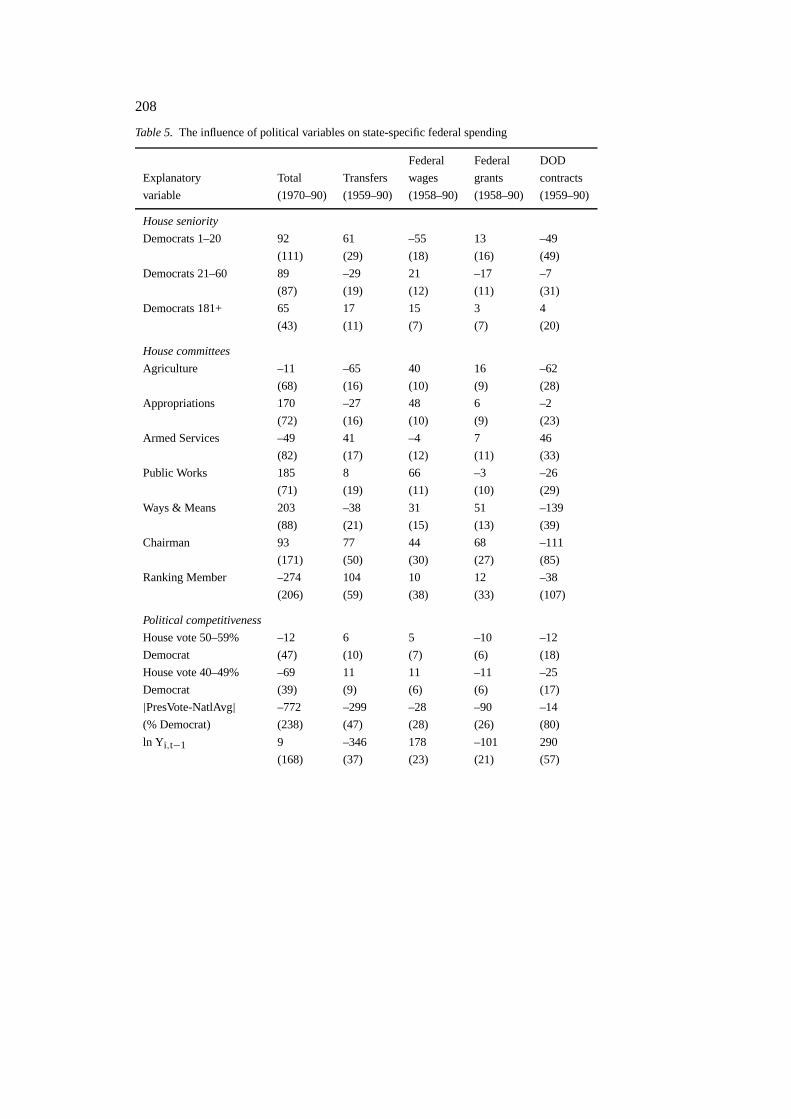
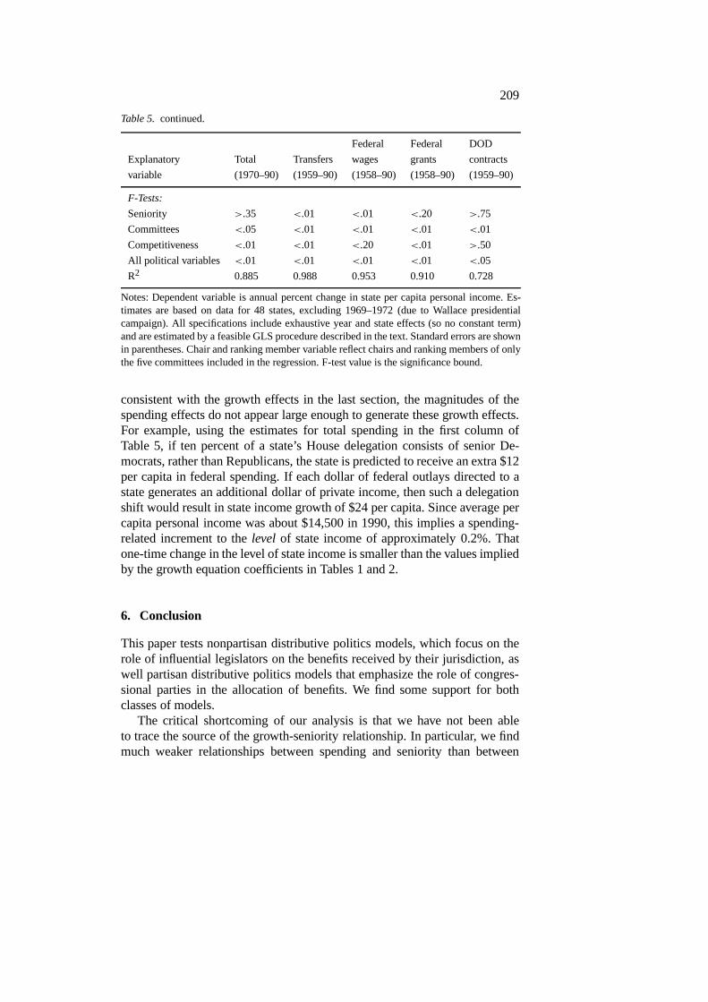
We estimate equations similar to those in the last section, substituting percapita federal spending (or a sub-category of spending) for economic growthrates as the dependent variable, maintaining the same independent variables.Table 5 presents estimates of these equations, with mixed results. For totalfederal outlays (column 1), the indicator variables for senior Democratic con-gressmen enter positively, but the estimated coefficients are not statisticallysignificant. The point estimates for individual spending categories show bothpositive and negative effects, but the null hypothesis of zero effect is rarelyrejected. Similarly, the coefficients on committee membership and commit-tee rank do not exhibit any clear pattern. The variables measuring politicalcompetition based on congressional vote percentages do not suggest higherspending in more competitive states, while the analogous variable based onpresidential vote share does suggest such an effect. For total spending andseveral spending categories, this effect is statistically significant.

The equations reported in Table 5 focus on the contemporaneous relation-ship between political factors and state economic growth. We also consideredthe possibility thatpastpolitical variables could affect current spending, sincethere may be lags between authorizations, appropriations, and expenditures.Moreover, the geographic pattern in some spending may be the result of pre-vious decisions, such as the location of military bases. We did not, however,find any systematic patterns when we added lagged political variables to ourspending equations. We also estimated equations relatingchangesin spend-ing to our SENIORITY, COMMITTEE, and COMPETITION variables, torecognize the possibility that current representatives might be unable to affectthe history-based level of spending, but could affect increments to it. Virtu-ally none of the political variables were statistically significant at standardsignificance levels in the spending change equations.

These results are puzzling in light of our earlier findings, for two reasons.First, since the political variables that are correlated with growth rates do notappear to be correlated with federal spending, these results raise the questionof what explains the link between political factors and economic growth.Second, even when the estimated coefficients in the spending equations are

208

Table 5. The influence of political variables on state-specific federal spending

Federal Federal DOD

Explanatory Total Transfers wages grants contracts

variable (1970–90) (1959–90) (1958–90) (1958–90) (1959–90)

House seniority

Democrats 1–20 92 61 –55 13 –49

(111) (29) (18) (16) (49)

Democrats 21–60 89 –29 21 –17 –7

(87) (19) (12) (11) (31)

Democrats 181+ 65 17 15 3 4

(43) (11) (7) (7) (20)

House committees

Agriculture –11 –65 40 16 –62

(68) (16) (10) (9) (28)

Appropriations 170 –27 48 6 –2

(72) (16) (10) (9) (23)

Armed Services –49 41 –4 7 46

(82) (17) (12) (11) (33)

Public Works 185 8 66 –3 –26

(71) (19) (11) (10) (29)

Ways & Means 203 –38 31 51 –139

(88) (21) (15) (13) (39)

Chairman 93 77 44 68 –111

(171) (50) (30) (27) (85)

Ranking Member –274 104 10 12 –38

(206) (59) (38) (33) (107)

Political competitiveness

House vote 50–59% –12 6 5 –10 –12

Democrat (47) (10) (7) (6) (18)

House vote 40–49% –69 11 11 –11 –25

Democrat (39) (9) (6) (6) (17)

|PresVote-NatlAvg| –772 –299 –28 –90 –14

(% Democrat) (238) (47) (28) (26) (80)

ln Yi,t−1 9 –346 178 –101 290

(168) (37) (23) (21) (57)

209

Table 5. continued.

Federal Federal DOD

Explanatory Total Transfers wages grants contracts

variable (1970–90) (1959–90) (1958–90) (1958–90) (1959–90)

F-Tests:

Seniority >.35 <.01 <.01 <.20 >.75

Committees <.05 <.01 <.01 <.01 <.01

Competitiveness <.01 <.01 <.20 <.01 >.50

All political variables <.01 <.01 <.01 <.01 <.05

R2 0.885 0.988 0.953 0.910 0.728

Notes: Dependent variable is annual percent change in state per capita personal income. Es-timates are based on data for 48 states, excluding 1969–1972 (due to Wallace presidentialcampaign). All specifications include exhaustive year and state effects (so no constant term)and are estimated by a feasible GLS procedure described in the text. Standard errors are shownin parentheses. Chair and ranking member variable reflect chairs and ranking members of onlythe five committees included in the regression. F-test value is the significance bound.

consistent with the growth effects in the last section, the magnitudes of thespending effects do not appear large enough to generate these growth effects.For example, using the estimates for total spending in the first column ofTable 5, if ten percent of a state’s House delegation consists of senior De-mocrats, rather than Republicans, the state is predicted to receive an extra $12per capita in federal spending. If each dollar of federal outlays directed to astate generates an additional dollar of private income, then such a delegationshift would result in state income growth of $24 per capita. Since average percapita personal income was about $14,500 in 1990, this implies a spending-related increment to thelevel of state income of approximately 0.2%. Thatone-time change in the level of state income is smaller than the values impliedby the growth equation coefficients in Tables 1 and 2.

6. Conclusion

This paper tests nonpartisan distributive politics models, which focus on therole of influential legislators on the benefits received by their jurisdiction, aswell partisan distributive politics models that emphasize the role of congres-sional parties in the allocation of benefits. We find some support for bothclasses of models.

The critical shortcoming of our analysis is that we have not been ableto trace the source of the growth-seniority relationship. In particular, we findmuch weaker relationships between spending and seniority than between

210

growth and seniority; this raises the question of whether the correlation be-tween growth and political factors is the result of correlation with other omit-ted variables. Searching for such omitted factors, especially for correlates ofstate political competitiveness, is a natural direction for future work. Alter-natively, the growth-seniority relationship may arise from factors other thanspending that are under congressional control. Regulatory and trade policies,or tax rules, are potential examples. We are not aware of any quantitativemeasures of the impact of these policies on states or congressional districts,so we have not been able to construct appropriate empirical tests.

The findings in this paper suggest a number of directions for further re-search. One concerns the link between congressional institutions and theoverall level of economic growth. While we focus on congressional represen-tation and the distribution of economic growth, there may also be importantinteractions between congressional structure and the likelihood of enactinglegislation that raises overall economic growth. There is a long-standing de-bate on the efficiency cost of pork-barrel type projects from the standpoint ofthe economy as a whole.

Another, more fundamental, question, is why voters ever elect representa-tives from parties that they expect will hold the minority position, or unilat-erally impose term limits on their state’s congressional delegation. If havingsenior representatives in the majority party is in fact correlated with morerapid state growth, then voters who elect representatives from the minorityparty are choosing lower growth. This may be explained by ideological pref-erences or other factors, but the interrelationships among these factors needto be formalized.

Notes

1. Universalism suggests a complex relationship between a legislator’s committee assign-ment and policy outcomes, and in practice it has proven difficult to test such relationships.Recent attempts include Collie (1988), Krehbiel (1991), and Stein and Bickers (1995).Baron’s (1989) study of congressional support for Amtrak is notable for the relativelyclear evidence it provides for a majoritarian rather than universal coalition on a cleardistributive politics issue.

2. Recent research, such as Weingast and Marshall (1988), Gilligan and Krehbiel (1990), andKrehbiel (1991), has focused on explaining the institutional structure of Congress. It is notclear whether data on the geographical distribution of economic benefits can differentiateamong alternative theories.

3. Wright (1974) and Fleck (1994) suggest that FDR pursued such a strategy, allocating thebenefits of New Deal programs toward marginal Democratic states.

4. We assume that spending raises support for the incumbent, despite Peltzman’s (1992)claim that governors who spend more are penalized by the voters. His evidence is notinconsistent with the possibility that voters penalize legislators who vote for high levels

211

of overall government expenditure, while rewarding legislators who maximize the shareof a fixed pool of federal dollars flowing toward their district.

5. Our analysis follows a voluminous literature on the determinants of economic growthrates, surveyed by Barro and Sala-i-Martin (1995).

6. If a congressman boosts economic activity, this may attract new residents to his district,and lead to a subsequent change in the district boundaries. This raises the possibilityof non-randomness in the set of congressional districts with constant boundaries acrossredistricting years.

7. Our specification assumes that representatives in small and large states have the sameability to affect district income. To illustrate this, consider a one-representative state,with its lone representative in the most senior group of Democrats. Then DEM1–20 willequal 1.0, and the effect on state per capita income growth will beα1. If a state has tenrepresentatives, and one is in the most senior group, his effect onstateper capita incomegrowth will be α1/10. The value of DEM1–20 for a state with one such representativewould be .10. In both cases, d(1ln Y)/d(DEM1–20) =α1.

8. The set of influential committees can vary over time. The House Ways and Means Com-mittee was probably more powerful before the 1974 House reforms that shifted some ofits functions to the Steering and Policy Committee.

9. Shepsle (1978) and Smith and Deering (1984) find that perceived constituent interests arethe strongest determinants of committee requests by newly-elected members of the House.Krehbiel (1990, 1991) argues that the process of allocating members to committees doesnot lead those from high-demand jurisdictions to occupy committee places.

10. We omit the years 1969–1972 from all regressions involving our political competitivenessvariable because of uncertainty over how to classify Wallace votes in the 1968 election.

11. We could not reject the null hypothesis of serial independence of the errors in models withlagged state per capita income.

12. The null hypothesis that the coefficients on the state fixed effects are zero is rejectedat standard confidence levels. We have also estimated Model 3 excluding the Southernstates. The estimated coefficients on the seniority variables are slightly larger, and differfrom zero at higher levels of statistical confidence, than those for the entire sample.

13. Some might argue that the very information removed by the state effects, the state averagegrowth rate and average seniority, should be the focus of our analysis. When we estimatedour regression models on state averages, we found coefficient estimates of the same signthat we find using the within variation, but the standard errors were typically too large topermit any strong inferences.

14. These specifications assume that the effect of deviations from the national average vote forpresident is the same regardless of whether it is skewed toward Democrats or Republicans.We could not reject this assumption.

15. One potentially important shift between the first and second parts of our sample is achange in the composition of senior Democratic House members. The share of suchmembers who represent urban areas in the North increased substantially during the sampleperiod, and this could contribute to differences in their estimated growth effects across thetwo subsamples.

16. While these effects on growth rates may appear inconsequential, even these small dif-ferences in growth rates can compound to generate large differences in the level of stateincome over time. For instance, our estimates imply that per capita income would havebeen over $800 lower in Texas by the end of our sample if it were the case that Texas hadaverage seniority over the period 1953–1990.

212

17. Existing empirical evidence suggests at best a weak link between state or district leveleconomic performance and votes cast for incumbent legislators. Kiewiet (1983) sug-gests that “national assessments” of the economy play a more important role in votesfor Congress than “personal experiences” based on the local economy. Erickson (1990)and Peltzman (1990) find that national economic conditions affect votes for incumbentcongressmen. This effect appears to be mediated largely by party membership. When thenational economy is strong, members of the President’s party receive an electoral benefit.Adams and Kenny (1989), Chubb (1988), and Peltzman (1987) find very small effectsof state economic performance on the re-election prospects of governors; Bennett andWiseman (1991) find small effects for senators.

18. After removing fixed year effects from the growth rates in personal income for all states,the serial correlation coefficient for state economic growth rates is approximately .05.

19. In an earlier version of this paper, we estimated reduced form models for Congressionaldelegation turnover as a function of state growth rates. We found a weak positive asso-ciation, consistent with the previous literature, but this link does not appear to be strongenough to explain our observed seniority-growth correlation.

20. Atlas et al. (1995) is an example of a recent study thatdoesfind an impact of politicalrepresentation, in this case a state’s degree of over-representation in Congress relative toits population, on federal outlays.

References

Adams, J.D. and Kenny, L.W. (1989). The retention of state governors.Public Choice62 (1):1–13.

Advisory Council on Intergovernmental Relations (1992).Significant features of fiscalfederalism, Volume 2: Revenues and expenditures. Washington: ACIR.

Atlas, C.M., Gilligan, T.W., Hendershott, R.J. and Zupan, M.A. (1995). Slicing the federalgovernment net spending pie: Who wins, who loses, and why.American Economic Review85(3): 624–629.

Baron, D.P. (1989). Distributive politics and the persistence of Amtrak.Journal of Politics52:883–913.

Baron, D.P. (1991). Majoritarian incentives, pork barrel programs, and procedural control.American Journal of Political Science35: 57–90.

Barro, R. and Sala-i-Martin, X. (1995).Economic Growth. New York: McGraw Hill.Bennett, R.W. and Wiseman, C. (1991). Economic performance and U.S. senate elections,

1958–1986.Public Choice69 (1): 93–100.Blanchard, O.J. and Katz, L. (1992). Regional evolutions.Brookings Papers on Economic

Activity1: 1–75.Chubb, J.E. (1988). Institutions, the economy, and the dynamics of state elections.American

Political Science Review82: 135–154.Coker, D.C. and Crain, W.M. (1994). Legislative committees as loyalty-generating institu-

tions.Public Choice81 (3–4): 195–221.Collie, M. (1988). The rise of coalition politics: Voting in the U.S. house, 1933–1980.

Legislative Studies Quarterly13: 321–342.Cox, G.W. and McCubbins, M.D. (1993).Legislative leviathan: Party government in the

house. Berkeley, CA: University of California Press.

213

Crain, W.M. and Tollison, R.D. (1977). The influence of representation on public policy.Journal of Legal Studies6 (2): 355–362.

Crain, W.M. and Tollison, R.D. (1981). Representation and influence: A reply.Journal ofLegal Studies10 (1): 215–219.

Erikson, R. (1990). Economic conditions and the congressional vote: A review of themacrolevel evidence.Journal of Politics50: 373–399.

Ferejohn, J. (1974).Pork barrel politics: Rivers and harbors legislation, 1947–1968. Stanford,CA: Stanford University Press.

Fiorina, M. (1981). Universalism, reciprocity, and distributive policy-making in majority ruleinstitutions. In J.P. Crecine (Ed.),Research in public policy making and management1:193–221.

Fleck, R. (1994). Essays on the Political Economy of the New Deal. Ph.D. dissertation,Stanford University Economics Department.

Gilligan, T. and Krehbiel, K. (1990). Organization of informative committees by a rationallegislature.American Journal of Political Science34: 531–564.

Goss, C.F. (1972). Military committee membership and defense-related benefits in the houseof representatives.Western Political Quarterly25: 215–233.

Greene, K.V. and Munley, V.G. (1980). The productivity of legislators’ tenure: A case lackingin evidence.Journal of Legal Studies10: 207–219.

Kiel, L.J. and McKenzie, R.B. (1983). The impact of tenure on the flow of federal benefits toSMSAs.Public Choice41: 285–293.

Kiewiet, D.R. (1983).Macroeconomics and micropolitics. Chicago: University of ChicagoPress.

Kiewiet, D.R. and McCubbins, M.D. (1991).The logic of delegation: Congressional partiesand the appropriations process. Chicago: University of Chicago Press.

Krehbiel, K. (1990). Are congressional committees composed of preference outliers?Ameri-can Political Science Review84: 149–163.

Krehbiel, K. (1991).Information and legislative organization. Ann Arbor: University ofMichigan Press.

Pearson, D. and Anderson, J. (1968).The case against congress: A compelling indictment ofcorruption on capitol hill. New York: Simon & Schuster.

Peltzman, S. (1987). Economic conditions and gubernatorial elections.American EconomicReview, Papers and Proceedings77: 293–297.

Peltzman, S. (1990). How efficient is the voting market?Journal of Law and Economics33:27–64.

Peltzman, S. (1992). Voters as fiscal conservatives.Quarterly Journal of Economics107: 327–361.

Ray, B.A. (1980). Congressional promotion of district interests: Does power on the hill reallymake a difference? In B. Rundquist (Ed.),Political benefits: Empirical studies of americanpublic programs, 1–35. Lexington, MA: Lexington Books.

Ray, B.A. (1981). Military committee membership in the house of representatives and theallocation of defense department outlays.Western Political Quarterly34: 222–234.

Reiselbach, L.N. (1986).Congressional reform. Washington: Congressional Quarterly Press.Ritt, L.G. (1976). Committee position, seniority, and the distribution of government expendi-

tures.Public Policy24: 469–497.Roberts, B.E. (1990). A dead senator tells no lies: Seniority and the distribution of federal

benefits.American Journal of Political Science34: 31–58.Rohde, D.W. (1991).Parties and leaders in the postreform house. Chicago: University of

Chicago Press.

214

Rundquist, B.S. (1978). On testing a military industrial complex theory.American PoliticsQuarterly6: 29–53.

Rundquist, B.S. and Griffith, D.E. (1976). An interrupted time-series test of the distributivetheory of military policy-making.Western Political Quarterly29: 620–626.

Shepsle, K.A. (1978).The giant jigsaw puzzle: Democratic committee assignments in themodern house. Chicago: University of Chicago Press.

Shepsle, K.A. and Weingast, B.R. (1994). Positive theories of congressional institutions.Legislative Studies Quarterly19 (2).

Smith, S. and Deering, C. (1984).Committees in congress. Washington: CongressionalQuarterly Press.

Snyder, J.M., Jr. (1994). Safe seats, marginal seats, and party platforms: The logic of platformdifferentiation.Economics and Politics6 (3): 201–213.

Stein, R.M. and Bickers, K.N. (1995).Perpetuating the Pork Barrel: Political Subsystems andAmerican Democracy. New York: Cambridge University Press.

Weingast, B.R. (1979). A rational choice perspective on congressional norms.AmericanJournal of Political Science23: 245–262.

Weingast, B.R. and Marshall, W.J. (1988). The industrial organization of congress; or, whylegislatures, like firms, are not organized as markets.Journal of Political Economy96 (1):132–163.

Wright, G. (1974). The political economy of new deal spending: An econometric analysis.Review of Economics and Statistics56: 30–38.

215

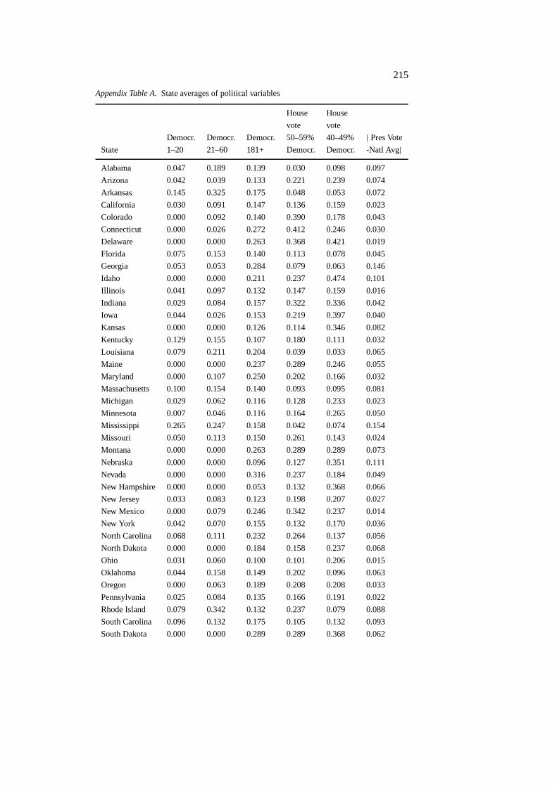
Appendix Table A.State averages of political variables

House House

vote vote

Democr. Democr. Democr. 50–59% 40–49%| Pres Vote

State 1–20 21–60 181+ Democr. Democr. -Natl Avg|Alabama 0.047 0.189 0.139 0.030 0.098 0.097

Arizona 0.042 0.039 0.133 0.221 0.239 0.074

Arkansas 0.145 0.325 0.175 0.048 0.053 0.072

California 0.030 0.091 0.147 0.136 0.159 0.023

Colorado 0.000 0.092 0.140 0.390 0.178 0.043

Connecticut 0.000 0.026 0.272 0.412 0.246 0.030

Delaware 0.000 0.000 0.263 0.368 0.421 0.019

Florida 0.075 0.153 0.140 0.113 0.078 0.045

Georgia 0.053 0.053 0.284 0.079 0.063 0.146

Idaho 0.000 0.000 0.211 0.237 0.474 0.101

Illinois 0.041 0.097 0.132 0.147 0.159 0.016

Indiana 0.029 0.084 0.157 0.322 0.336 0.042

Iowa 0.044 0.026 0.153 0.219 0.397 0.040

Kansas 0.000 0.000 0.126 0.114 0.346 0.082

Kentucky 0.129 0.155 0.107 0.180 0.111 0.032

Louisiana 0.079 0.211 0.204 0.039 0.033 0.065

Maine 0.000 0.000 0.237 0.289 0.246 0.055

Maryland 0.000 0.107 0.250 0.202 0.166 0.032

Massachusetts 0.100 0.154 0.140 0.093 0.095 0.081

Michigan 0.029 0.062 0.116 0.128 0.233 0.023

Minnesota 0.007 0.046 0.116 0.164 0.265 0.050

Mississippi 0.265 0.247 0.158 0.042 0.074 0.154

Missouri 0.050 0.113 0.150 0.261 0.143 0.024

Montana 0.000 0.000 0.263 0.289 0.289 0.073

Nebraska 0.000 0.000 0.096 0.127 0.351 0.111

Nevada 0.000 0.000 0.316 0.237 0.184 0.049

New Hampshire 0.000 0.000 0.053 0.132 0.368 0.066

New Jersey 0.033 0.083 0.123 0.198 0.207 0.027

New Mexico 0.000 0.079 0.246 0.342 0.237 0.014

New York 0.042 0.070 0.155 0.132 0.170 0.036

North Carolina 0.068 0.111 0.232 0.264 0.137 0.056

North Dakota 0.000 0.000 0.184 0.158 0.237 0.068

Ohio 0.031 0.060 0.100 0.101 0.206 0.015

Oklahoma 0.044 0.158 0.149 0.202 0.096 0.063

Oregon 0.000 0.063 0.189 0.208 0.208 0.033

Pennsylvania 0.025 0.084 0.135 0.166 0.191 0.022

Rhode Island 0.079 0.342 0.132 0.237 0.079 0.088

South Carolina 0.096 0.132 0.175 0.105 0.132 0.093

South Dakota 0.000 0.000 0.289 0.289 0.368 0.062

216

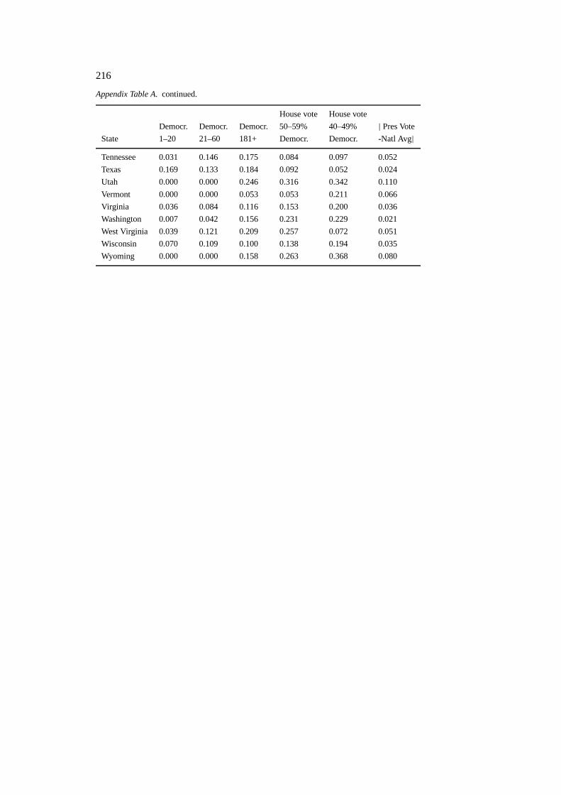
Appendix Table A.continued.

House vote House vote

Democr. Democr. Democr. 50–59% 40–49% | Pres Vote

State 1–20 21–60 181+ Democr. Democr. -Natl Avg|Tennessee 0.031 0.146 0.175 0.084 0.097 0.052

Texas 0.169 0.133 0.184 0.092 0.052 0.024

Utah 0.000 0.000 0.246 0.316 0.342 0.110

Vermont 0.000 0.000 0.053 0.053 0.211 0.066

Virginia 0.036 0.084 0.116 0.153 0.200 0.036

Washington 0.007 0.042 0.156 0.231 0.229 0.021

West Virginia 0.039 0.121 0.209 0.257 0.072 0.051

Wisconsin 0.070 0.109 0.100 0.138 0.194 0.035

Wyoming 0.000 0.000 0.158 0.263 0.368 0.080