Embed Size (px)
Citation preview

Consequences of booking
market-driven goodwill Impairments
Presented by
Dr Pervin Shroff
Professor Carl L Nelson Professorship in Accounting
University of Minnesota
#2013/14-05
The views and opinions expressed in this working paper are those of the author(s) and not necessarily those of the School of Accountancy, Singapore Management University.

Consequences of booking market-driven goodwill impairments*
Wen Chen University of Minnesota
Pervin K Shroff University of Minnesota
Ivy Zhang University of Minnesota
May 2013
Preliminary
*We thank Peter Easton, Frank Gigler, Zhaoyang Gu, and participants of the University of Minnesota Empirical Conference for helpful comments and suggestions.

Consequences of booking market-driven goodwill impairments
Abstract
Under the fair-value-based goodwill impairment test of SFAS 142, a firm’s market value is often used as an important reference point for determining the existence of impairment. In fact, a below-one market-to-book ratio is considered by many, including external auditors and security lawyers, to be an indicator of goodwill impairment. As a result, firms can be pressured into recording goodwill impairment upon a temporary market value decline which is unsubstantiated by economic fundamentals. From a sample of goodwill impairments recorded during the period 2002-2009, we identify about a sixth of the sample firms which report impairment charges that are most likely market-driven and not backed by fundamentals. Validating our identification of market-driven impairments, we find that the impairment loss of these firms is associated with a return reversal in the subsequent year. It appears from our results that the market does not understand the difference between market-driven and other impairments and reacts equally negatively upon the initial announcement of the loss, resulting in a further price decline for firms with market-driven impairment. In addition, we find that, until the return reversal occurs, firms with market-driven impairment experience an increase in information asymmetry associated with the impairment loss. Finally, our results suggest that the managers of these firms exploit the delay in the market's reversal of the temporary undervaluation related to the impairment by engaging in share repurchases to a greater extent than normal. Overall, our findings shed light on the potential negative consequences of the imperfect implementation of fair value accounting.

1
1. Introduction
The Statement of Financial Accounting Standards (SFAS) No. 142, Goodwill and Other Intangible
Assets, issued by the Financial Accounting Standards Board (FASB), effective July 2001, requires
companies to review goodwill for impairment at annual intervals and when triggering events occur,
and to recognize a loss if goodwill is impaired. As an immediate consequence of this standard, there
was a spate of goodwill write-offs running into millions of dollars announced by a number of high-
profile companies, such as AOL Time Warner. A second wave of goodwill write-offs occurred
during the recent recession and market collapse with impairment charges amounting to roughly two-
thirds of the goodwill balance on companies’ opening balance sheets (Comiskey and Mulford 2010).
SFAS 142 requires companies to determine the goodwill impairment loss using a fair value approach.
Specifically, the fair value of goodwill is determined as the residual fair value of a reporting unit
after subtracting the fair value of its recognized net assets other than goodwill. To determine fair
values, SFAS 142 suggests that quoted market prices provide the best evidence of fair values.
Consistently, a subsequent standard, SFAS 157 (updated), Fair Value Measurements, specifies the
fair value hierarchy and emphasizes that “level 1” fair value measurement reflects values from
orderly transactions.
Given SFAS 142’s prescription on fair value measurement and emphasis on impairment
triggers, it is quite likely that goodwill impairment losses taken by firms are based on a current
decline in firms’ market values.1 While a firm’s market value provides an objective measure of the
combined fair values of reporting units, it can temporarily deviate from the firm’s fundamental value
for various reasons, including volatile markets, illiquidity, price pressure, exogenous shocks and
1 Although SFAS 142 does not specifically refer to a decline in market prices as an example of a triggering event, International Accounting Standard (IAS) 36, Impairment of Assets, lists market value decline as an external indicator of impairment. Also, major public accounting firms in the U.S. consider a significant stock price decline to be a potential impairment trigger (Dharan 2009). Based on a sample of firms that took a goodwill write-off in 2008, Comiskey and Mulford (2010) find that 68% of the firms viewed a decline in equity prices as a goodwill impairment triggering event.

2
other market frictions. Due to pressure from external auditors and/or litigation concerns, firms
experiencing a temporary decline in their market value may be forced to recognize a goodwill
impairment loss even in the absence of any evidence of economic impairment in fundamentals. As a
consequence, market prices can be further distorted if investors fail to understand the nature of the
impairment loss. In this paper, we identify cases of goodwill impairment that are likely driven by the
market-based impairment signal but not backed by economic fundamentals. We first examine
whether these firms experience a price reversal associated with the impairment in the subsequent
year. We then test whether the market is misled by these impairments, how the impairment
recognition affects the information environment, and whether managers exploit the impairment-
related undervaluation by taking actions such as repurchasing shares.
We categorize a firm in the impairment sample as recording a “market-driven non-
fundamental” impairment if its market performance signals impairment but the firm’s fundamentals
do not indicate an economic impairment.2 We consider the market signal of impairment to be strong
if the ratio of a firm’s market value of equity to book value of equity (M/B) declines during the year
and is less than one at the end of the year.3 To determine whether a firm’s fundamentals signal
goodwill impairment, we construct a composite measure of firm fundamentals by conducting a factor
analysis of various current and expected future performance indicators for the Compustat population
during our sample period. We then categorize firms that fall in the bottom tercile of the distribution
based on the sum of the first two factors as exhibiting weak fundamentals suggestive of economic
2 In the interest of brevity, we also refer to market-driven non-fundamental goodwill impairments simply as market-driven impairments in subsequent discussions. 3 Several prior studies have used M/B less than 1 as an indicator of potential goodwill impairment (e.g., Beatty and Weber 2006, and Ramanna and Watts 2012). As discussed in the next section, a below-one market-to-book ratio is also considered by regulators, public accounting firms, and security lawyers as a signal of goodwill impairment.
3
impairment.4 To (ex post) validate that the goodwill impairment of these firms is related to a
temporary price decline, we begin by examining whether the market later reverses its effect.
Specifically, we test whether the magnitude of the impairment is positively correlated with the
subsequent year’s returns.
We estimate a regression of the subsequent year’s market-adjusted returns on the magnitude
of the impairment interacted with indicator variables for the market-driven impairment sample and
benchmark impairment samples (along with other determinants of returns). We use several
benchmark samples to establish our results. First, we use all impairment firms other than firms with
market-driven non-fundamental impairment as a benchmark sample. Our second benchmark sample
includes only impairment firms that have “confirmatory” signals, that is, both the market and
fundamental impairment signals are consistently negative, thus indicating a higher likelihood of an
economic impairment. We believe that these impairments are less likely to be “forced” by a
temporary market decline since the firm’s fundamentals also corroborate an economic impairment.
Our results indicate a significant return reversal for the market-driven impairment sample, but none
for the benchmark impairment samples, confirming that the impairment of the market-driven sample
is related to a temporary price decline.
The positive association between subsequent returns and the impairment magnitude of the
market-driven sample does not necessarily imply that the market is misled by the recognition of the
impairment charge. This is because the positive association could capture either the reversal of the
market’s negative reaction to the impairment announcement or prior negative returns that led to the
impairment or both. We therefore test whether the market was initially misled into reacting
negatively to the announcement of the impairment. Our results show a significant negative reaction
4 For the factor analysis, we use the level of return on assets (ROA), operating cash flows, and gross margin as indicators of current performance, and changes in ROA, operating cash flows, gross margin, sales, capital expenditure, and the number of employees as indicators of expected future performance. The first factor captures the levels variables which we interpret as current performance, and the second factor captures changes in variables which we interpret as indicators of trends in future performance.

4
to market-driven impairment announcements which is not distinguishable from that of the benchmark
impairment samples. Thus, the market does not appear to understand that these impairments are not
backed by fundamentals leading to further undervaluation upon their announcement.
The market is likely to understand the nature of these impairments when later realizations
provide confirmatory information. To determine the point in time during the subsequent year when
the price reversal occurs, we analyze (cumulative) quarterly patterns in the relation between the
magnitude of impairment and returns in the subsequent year. We find an insignificant relation
between impairment and subsequent returns up to the end of three quarters, and a significant positive
relation only in the fourth quarter. Thus, our evidence suggests that the market learns about the
undervaluation (at least partially) only when the next year’s performance results are released.
Since the market recognizes the nature of market-driven impairments with a delay, we expect
to observe several consequences associated with this delay. First, we hypothesize that the
recognition of impairment in the presence of conflicting signals (i.e., market versus fundamental)
will lead to greater uncertainty about the stated value of goodwill and its future cash flow
implications. Hence, we expect to observe more diverse interpretations of this information by market
participants as captured by an increase in the bid-ask spread and analysts’ forecast dispersion in the
interim period. Second, we expect managers to have private information about the “true” value of
goodwill and therefore hypothesize that they will take actions in the interim period to take advantage
of the market’s undervaluation of goodwill and its implications for future cash flows. Thus, based on
the timing of the market’s correction, we test whether the managers of these firms repurchase more
shares in the interim period relative to benchmark firms.
In analyzing the consequences of the lag in the market’s recognition of the nature of these
impairments, we examine the relation between the magnitude of impairment and commonly used
measures of information asymmetry in the subsequent year for the market-driven impairment sample
5
relative to the benchmark impairment samples. We find an incremental positive relation between
impairment magnitude and the change in bid-ask spreads and analysts’ forecast dispersion for the
market-driven impairment sample, suggesting an increase in information asymmetry for these firms
associated with the previously recorded goodwill impairment. We also compare the market-driven
impairment sample with a matched control sample of non-impairment firms. For each impairment
firm, we identify one non-impairment control firm that belongs to the same industry and has similar
levels of market and fundamental indicators as the impairment firm. Market-driven impairment
firms exhibit a greater increase in information asymmetry associated with the impairment relative to
control firms, suggesting that the recognition of impairment exacerbates information asymmetry.
We also find evidence suggesting that managers take advantage of the temporary under-
pricing of their firm’s shares due to market-driven goodwill impairments. In the subsequent year, we
find that, relative to the benchmark impairment samples, there is a significantly higher correlation
between the magnitude of impairment and the firm’s propensity to repurchase for the market-driven
impairment sample; also, the correlation between impairment magnitude and the dollar amount
repurchased is significantly higher for these firms relative to the benchmark firms. Further,
compared to matched control firms with similar levels of market and fundamental indicators, market-
driven impairment firms exhibit an incremental tendency to repurchase that is positively correlated
with the magnitude of impairment. Thus, it appears that insiders are aware that these impairments
are induced mainly by a temporary market decline in their stock, and moreover realize that the
market is not aware of the nature of these impairments at least for a while. As a consequence, they
buy back their own shares at a price lower than that indicated by fundamentals and at the same time
signal their firm’s undervaluation to the market.
From our results, goodwill impairment charges taken by a sixth of our sample companies are
likely driven by the decline in their market prices, unsubstantiated by fundamentals. We find that the

6
frequency of such market-driven impairments more than doubles during the financial crisis when a
significant number of firms experience temporary slumps in the price of their stock. Investors at
least temporarily are unable to distinguish these impairments from those that reflect impaired
economic fundamentals. The accounting recognition of market-driven impairments results in a
further price decline, suggesting that the fair-value-based accounting for goodwill exacerbates the
severity of mispricing particularly in times of crisis. Although it appears that managers are aware of
the nature of these impairments, the rules prohibit them from reversing a previously recorded
impairment loss under any circumstances. As a consequence of this prohibition, the price distortion
may persist until subsequent news confirms that the impairment charge was inconsistent with
economic fundamentals.
Our paper contributes to the literature investigating the effect of goodwill impairment losses
based on fair value measurement. The use of unverifiable fair values in estimating goodwill
impairment has been questioned by Ramanna and Watts (2012). These authors provide evidence
suggesting that a number of firms with potentially impaired goodwill (on the basis of M/B) did not
take an impairment charge, probably justified by subjective fair values of reporting units. Different
from Ramanna and Watts (2012), we focus on firms that may have been “forced” to take an
impairment charge because of a so-called objective fair-value criterion. We provide evidence
suggesting that firms who did take an impairment charge on the basis of a temporary decline in
equity prices may have misled the market. Our results focus on the flawed implementation of fair
value accounting in booking impairments rather than fair values facilitating impairment avoidance
and thus complement the findings of Ramanna and Watts (2012). On the one hand, the use of
unverifiable fair values may encourage managers to behave opportunistically; on the other hand,
blind adherence to fair value prescriptions while disregarding the underlying economics of the
situation can swing the pendulum to the other extreme and also result in misleading investors.

7
Our paper also sheds light on the role of fair value accounting in the recent financial crisis.
During the financial crisis, arguments were made that fair value accounting forced banks to write
down temporarily-depressed investments that they had no intention of selling, leading them to make
sub-optimal pro-cyclical actions that further amplified the crisis. While admittedly the impact of fair
value accounting was orders of magnitude greater in the financial sector, we provide evidence that
fair value accounting of the goodwill asset also had similar spiral effects on firms in the real
economy. Perhaps the FASB's revised guidance on fair value measurement addressing the use of
quoted prices in inactive markets will check the flawed implementation of fair value accounting in
future.
The rest of the paper is organized as follows. Section 2 describes the hypotheses. Section 3
discusses the data and variables. Research design and empirical results are reported in Section 4,
followed by concluding remarks in Section 5.
2. Hypotheses development
SFAS 142 requires that firms test goodwill for impairment annually and between annual tests if an
event occurs or circumstances change that would more likely than not reduce the fair value of a
reporting unit below its carrying amount (FASB, 2001). The impairment test is a two-step procedure
based on fair values. Step one involves comparing the fair value of a company’s reporting unit with
its carrying amount, including goodwill. If the carrying amount of a reporting unit exceeds its fair
value, the second step of the goodwill impairment test must be carried out to measure the amount of
the impairment loss, which equals the difference between the carrying amount of goodwill and its
estimated fair value.
The fair values used for goodwill impairment testing are generally not readily available and
have to be estimated. Yet, the market value of a firm provides an objective measure of the combined
8
fair values of reporting units and becomes an important factor to consider in the testing process. In
fact, it is widely viewed as a key indication of impairment if a firm’s market value falls below its
book value. Several academic studies identify firms with goodwill impairment using the market-to-
book ratio (e.g., Beatty and Weber 2006; Ramanna and Watts 2012). A below-one market-to-book
ratio is also considered by regulators and accounting firms as a signal of goodwill impairment.
While regulators emphasize that it is not the only factor to consider in assessing goodwill for
impairment, they point out that it is “prudent to reconcile the combined fair values of your reporting
units to your market capitalization.”5 In his presentation to the American Institute of Certified Public
Accountants (AICPA) in December 2008, Steven C. Jacobs, Associate Chief Accountant of the
Division of Corporation Finance at the Securities and Exchange Commission (SEC), specifically
listed “decline in market capitalization below book value” as an event that may trigger an interim
goodwill impairment test.6 McGladrey, the fifth largest accounting firm in the U.S. in terms of
revenue, states in their publication that while they do not believe a reduction of market capitalization
below book value is an “automatic indicator,” a significant decline in the market capitalization below
the carrying amount may be an event or circumstance that triggers the requirement for impairment
testing.7
While regulators and auditors are cautious and avoid using the market-to-book ratio as the
sole determinant of goodwill impairment, security lawyers place substantial emphasis on it in
evaluating if impairment has occurred. For example, Latham & Watkins, one of the largest law firms
in the world, recommends to its clients that in case their market capitalization is less than book value,
they should prepare for the possibility of goodwill impairment and ensure that appropriate
5 http://www.sec.gov/news/speech/2008/spch120808rgf.htm. 6 http://www.sec.gov/news/speech/2008/spch120908wc-slides.pdf 7 http://mcgladrey.com/pdf/goodwill_impairment_testing_today_economy.pdf

9
disclosures are made.8 This suggests that a below-one market-to-book ratio is associated with the
general perception that goodwill impairment exists. If a firm does not record a goodwill impairment
charge in the presence of a below-one market-to-book ratio, it can be targeted by security lawyers for
a class action lawsuit on account of its failure to record and disclose the loss.
Benchmarking against the market value of the firm likely constrains the subjectivity in the
goodwill impairment testing process. However, the relevance of the approach critically hinges on
market value conforming to economic fundamentals. If stock prices deviate from the underlying
economics for a variety of reasons, market value could be a misleading indicator of impairment. Yet,
SFAS 157 assigns quoted prices in active markets the highest priority (level 1) in estimating fair
values, with quoted prices in inactive markets and "unobservable inputs" assigned level 2 and level 3
priority, respectively. The strict enforcement of SFAS 157 by auditors is apparent from the 2007
white paper issued by the Center for Audit Quality (mainly representing the Big-4 accounting firms),
which emphasized that prices from inactive markets took precedence over internal cash flow
projections and pricing models. The legitimacy of fair-value accounting in the presence of less
active or inactive markets was questioned by many during the recent financial crisis in the context of
other assets and liabilities (e.g., investments and derivatives) of financial institutions in particular. It
appears that SFAS 157 and its interpretation may have helped auditors to force their clients to anchor
fair values on depressed prices from inactive markets even if those prices were not determinative of
fair value.9, 10
8 http://www.lw.com/upload/pubContent/_pdf/pub2484_1.pdf 9 In response to outside pressure during the crisis to amend fair value accounting, a subsequent FASB staff position (No. 157-4) allowed companies to depart from observable market values and use more optimistic fair value estimates. 10 In addition to auditors, the SEC has also pursued firms that did not write down investments based on a decline in their market values. While it is hard to imagine firms not complying with the SEC's directive, in a notable case of Berkshire Hathaway, the company's CFO communicated to the SEC that the company did not plan to write off losses on two of its investments because the prices did not reflect the worth of the shares (see Holm 2011).

10
Particular to goodwill impairment, if auditors consider M/B<1 to be a strong signal of
impairment, even though economic fundamentals indicate otherwise, firms can be forced to take an
impairment charge in the auditing process. In order to reduce litigation risk, firms may even
voluntarily record a goodwill impairment charge if their M/B ratio declines during the year and is
less than one at the end of the year. In this case, a goodwill impairment charge reflects a temporary
market value decline rather than declining economic fundamentals, i.e., an economic impairment.
We refer to these impairment charges taken in the presence of the market indicator (M/B<1 and
∆M/B<0) but not backed by economic fundamentals as “market-driven non-fundamental”
impairments (or market-driven impairments, for the sake of brevity).
We first ex post validate that market-driven impairments in fact reflect a market decline that
is temporary in nature. If the impairment is associated with temporary mispricing, we expect the
market to correct the mispricing subsequently as economic news is revealed. Thus, if our
identification of market-driven impairments is correct, we expect to observe a positive correlation
between subsequent returns and the impairment amount for this sample.
Prior research shows that announcements of goodwill impairment, on average, convey bad
news and cause investors to adjust their expectations about future cash flows downward (see Li et al.
2011, Bens et al. 2011). A consequence of booking goodwill impairment on the basis of a temporary
market decline is that the accounting recognition of the impairment may mislead the market into
reacting negatively and further undervaluing the stock. During the financial crisis, many blamed fair
value accounting for forcing banks to write down temporarily-depressed investments that they had no
intention of selling, leading them to make sub-optimal pro-cyclical actions resulting in a downward
spiral.11 While by no means comparable to its effect on the financial sector, we examine whether fair
11 Badertscher, Burks and Easton (2012) show that fair value accounting losses had minimal effect on commercial banks' regulatory capital during the crisis and that the (pro-cyclical) investment sales made by banks in response to these losses were economically insignificant. On the other hand, Bhatt, Frankel and Martin (2012) report results

11
value accounting had similar spiral effects on the real economy via its effect on the goodwill asset. If
investors do not immediately recognize that market-driven goodwill impairments reflect a temporary
decline in market values, the accounting recognition of the impairment could exacerbate the
undervaluation by leading to a further decline in the stock price. Thus, we test whether investors
react negatively upon the announcement of market-driven impairments and whether the reaction is
similar to that of other impairments.12 Our first hypothesis is the following:
H1: The market reacts negatively to the announcement of market-driven goodwill impairments
and the reaction is not significantly different from that of other goodwill impairments.
It is an empirical question as to how long it takes for the market to discover and correct the
temporary mispricing associated with market-driven goodwill impairment. As restoration of a
previous impairment charge is not allowed under the current reporting regime, managers cannot
effectively communicate their private information about the nature of the impairment to the market.
Instead, the mispricing is likely corrected over time with the revelation of economic news that
provides more information about the firm’s future cash flows. Theoretical models with imperfect
information predict that stock prices adjust to poor quality information gradually, not instantaneously
(e.g., Verrecchia 1980, Callen, Govindaraj, and Xu 2000, and Callen, Khan, and Lu 2012). When
accounting information is imprecise, for example in the case of market-driven goodwill impairments,
investors’ understanding of the implications of this information for future cash flows would evolve
over time, so that prices would reflect fundamentals with a delay. Thus, before sufficient economic
news is released to resolve the mispricing, we expect that firms with market-driven goodwill
impairment experience an increase in information asymmetry that is correlated with the magnitude of
suggesting that feedback between bank holdings of mortgage-backed securities and their market prices was aggravated by mark-to-market accounting and had a measurable effect on shareholder value. 12 Note that a positive association between subsequent returns and the impairment amount cannot be construed as evidence that investors were misled by the recognition of market-driven impairments. This is because the positive association could be due to the reversal of the price impact of the impairment announcement and/or the effect of prior (temporary) negative returns that led to the market-driven impairment.

12
impairment. We use bid-ask spreads as a proxy for information asymmetry among investors. This is
consistent with previous studies that argue that poor accounting and disclosure quality is associated
with wider spreads because it results in differentially informed investors and thus increases the
adverse selection risk of liquidity providers (Bhattacharya, Desai, and Venkataraman 2012, and
Heflin, Shaw, and Wild 2005). We also use dispersion in analysts’ forecasts as an additional proxy
for information asymmetry among market participants. Our second prediction is thus the following:
H2: Relative to benchmark firms, firms reporting market-driven impairments experience an
incremental increase in subsequent bid-ask spreads and analysts’ forecast dispersion that is
associated with the impairment.
There are several theoretical studies in behavioral corporate finance which model imperfect
capital markets in which investors are irrational but managers are able to identify price dislocations
(see Baker, Ruback, and Wurgler 2007 for a review). Consistent with theory, Brockman and Chung
(2001) find that managers use their private information about the firm’s undervaluation to time
equity repurchases in the open market. Since managerial wealth is tied to the value of the firm, it is
likely that managers will use their superior knowledge about their firm’s fundamentals to their own
advantage and that of existing shareholders. In the case of market-driven goodwill impairment, we
expect that managers would understand the temporary underpricing due to the market-driven
impairment charge and act to take advantage of the mispricing and/or to signal in order to correct the
mispricing. Specifically, we predict that, relative to benchmark firms, the impairment charge of
these firms will be associated with more share repurchases during the “window of opportunity,” i.e.,
in the period beginning with the impairment announcement until the market correction occurs. Thus,
our third prediction is the following:
H3: Relative to benchmark firms, firms reporting market-driven impairments exhibit an
incremental increase in stock repurchases that is associated with the impairment.

13
We use the sample of (i) non market-driven impairment firms, and (ii) “confirmatory”
impairment firms as benchmark samples to test these hypotheses. The confirmatory sample includes
impairments taken when both the market and the fundamental signals are present. Our purpose in
using the confirmatory impairment sample is to compare the effects of “forced” market-driven
impairments with economic impairments. Since both these groups have a declining and below-one
M/B, comparing the two groups controls for the impact of the market indicator on subsequent stock
returns and information asymmetry. In addition, we also use a sample of non-impairment control
firms as a relative benchmark in our tests of hypotheses 2 and 3. In the next section, we describe our
sample selection and descriptive statistics for the final sample.
3. Data and sample selection
3.1 Sample selection
We begin by selecting firms that report a goodwill impairment charge during the period 2002-09 as
recorded in Compustat. Our sample period begins in 2002, the year in which most firms adopted
SFAS 142. We obtain financial information from Compustat and price and return data from CRSP.
We exclude financial institutions (SIC 6000-6999) and utility firms (SIC 4900-4999), and require
sample firms to have (1) financial and stock price data for calculating the market and the
fundamentals indicators, and (2) financial and return data of the year subsequent to the impairment.
To mitigate the effect of outliers, we further exclude observations with market-adjusted returns
greater than 200%, penny stocks, and firms with negative market-to-book ratios from our sample.
After imposing these data requirements, we obtain a sample of goodwill impairments that includes
1,543 firm-year observations.
As discussed earlier, our hypotheses focus on “market-driven non-fundamental” goodwill
impairments, namely, impairment charges taken in the presence of the market indicator but not the
14
fundamentals indicator. To identify these impairments, we construct indicators of the market signal
and the fundamentals signal of goodwill impairment. Reflecting the popular belief that declining
market values and M/B<1 are strong signals of goodwill impairment, we base the market indicator on
the M/B ratio. Specifically, we consider the market indicator of goodwill impairment to be present
when a firm’s market value of equity relative to its book value of equity (after adding back the after-
tax impairment charge) declines during the year and falls below one at the end of the impairment
year (i.e., M/B<1 and ∆M/B<0).
We rely on accounting performance measures to capture the fundamentals indicator of
goodwill impairment. While accounting performance measures can be noisy or untimely in
reflecting economic fundamentals, they are less affected by temporary market shocks than stock
prices. We conduct a factor analysis using several variables that reflect firms’ current and expected
future performance. Specifically, we use the level of ROA, operating cash flows to total assets, and
gross margin as indicators of current performance. We include operating cash flows in addition to
ROA to ensure that the firm’s earnings performance is backed by cash generation from operations
and is therefore less likely to be simply a result of accruals manipulation. We further include change
in ROA, change in operating cash flows to total assets, change in gross margin, sales growth, capital
expenditure (scaled by total assets), change in capital expenditure, and change in the number of
employees as indicators of expected future performance. Changes in various performance variables
are expected to provide information about the trend in the firm’s future prospects. In addition, the
level and growth in capital expenditure and growth in employees capture the firm’s current and
future investment opportunities and are therefore considered to be indicators of the firm’s expected
future performance.
The factor analysis is performed using all Compustat firms that belong to the same industry
(two-digit SIC) as firms in the impairment sample with available data during the sample period. We

15
select the first two factors from the factor analysis -- the first factor captures the effect of three levels
variables (ROA, operating cash flows, and gross margin) which we interpret as a measure of current
performance, and the second factor captures the effect of changes in these three variables which we
interpret as a measure of the future trend in performance.13 For each firm-year observation, we
calculate the factor scores of the first two factors and measure the composite score as the sum of the
two factor scores. A firm is considered to have a fundamental signal of impairment if its composite
factor score falls in the bottom tercile of the distribution for all Compustat firms.14
Based on the indicators of impairment defined above, we identify 16% of sample firms as
experiencing market-driven non-fundamental impairment (with the market indicator but not the
fundamentals indicator of impairment), and 19% as experiencing confirmatory impairments (with
both the market and the fundamentals indicator of impairment).
As described above, we construct the market and fundamental indicators at the firm level,
whereas the actual impairment test is conducted at the reporting unit level. Although reporting unit level
indicators would be our ideal choice, data limitations compel us to rely on firm-level indicators. First, in
relation to the market indicator of impairment, note that reporting units generally are not traded
subsidiaries and hence the market value of a unit is not available. Second, as regards the fundamentals
indicator, we could potentially make use of segment-level disclosures to construct the fundamentals
indicator at the reporting unit level. However, our reading of 10-K reports for about 10% of our sample
reveals the following: the segment to which a reporting unit belongs is not always disclosed, the
allocation of impairment amounts to different segments is not always clear, and the segment profitability
measure that is disclosed is not consistently defined across firms. As a result, it is difficult to make use of
13The Appendix provides detailed results of the factor analysis. 14 We believe that classifying firms with fundamental scores in the bottom tercile as having poor fundamentals is justified since less than 10% of the Compustat population in our sample period reports goodwill impairment. The tenor of our results is unchanged if we instead classify firms with a below-median fundamental score as having low fundamentals suggestive of economic impairment.

16
segment-level data to construct the fundamentals indicator. We acknowledge that our use of firm-level
indicators may introduce noise in our identification of market-driven non-fundamental impairments;
however, the concern may not be as serious due to the following: (i) To the extent the performance of
reporting units is correlated and legal counsel/auditors advise managers to use the firm’s M/B ratio as an
indicator of impairment (as anecdotal evidence suggests), measurement error should be less of a concern.
(ii) Misclassification of market-driven non-fundamental impairment firms will bias against finding
differences between the samples. (iii) In sensitivity analysis, we test our hypotheses using only single-
segment firms for which firm-level measures are the appropriate indicators of impairment and find
substantially similar results. (iv) In additional sensitivity analysis, we eliminate, from the market-driven
impairment sample, firms with negative EPS in one or more segments and obtain substantially similar
results.
3.2 Matched control firms
One possible concern in testing for differences between market-driven and benchmark impairment
samples is that our results may be driven by the firm characteristics used to identify these impairment
subgroups. To mitigate this concern, we obtain a matched control sample of non-impairment firms
with reported goodwill at the beginning of the impairment year. We require the matched control
observation to be from the same year and the same industry (two-digit SIC) as the impairment firm
and to have the same market indicator of impairment (i.e., M/B<1 and ∆M/B<0 for market-driven
and confirmatory impairment firms and M/B>1 or ∆M/B>0 for the remaining impairment firms).15
Then, from non-impairment firms satisfying these requirements, we choose a control firm from the
same fundamentals-indicator category (i.e., bottom tercile or top two terciles) with the closest
fundamentals indicator (composite factor score) as the impairment firm.
15 For 12% of our sample firms, we obtain a matched control firm at the one-digit SIC code level, since the additional data requirements result in no match at the two-digit level.

17
3.3 Descriptive statistics of the impairment sample
Table 1 reports the distribution of the entire impairment sample by year and presents the descriptive
statistics of the impairment sample and its matched control sample. Panel A shows that 31% of
goodwill write-offs (473 firms) occur in 2008, right in the middle of the recent financial crisis,
consistent with significant economic impairment occurring during the accompanying recession.
To mitigate the undue impact of outliers, all continuous variables are winsorized at the top
and bottom 1% of their distribution. Panel B presents the mean and median characteristics of the
total impairment sample and the matched control sample of firms. The mean (after-tax) impairment
charge amounts to 5% of the market capitalization of the impairment sample. Compared to control
firms, the impairment firms are on average larger in size and have significantly lower ∆ROA, stock
returns, and M/B ratio. Although the composite fundamental factor score of the impairment sample
is lower than that of the control sample, the difference is insignificant. To compensate for the less
than perfect control-firm matching on impairment indicators, we also include these indicators as
control variables in our regressions.
3.4 Descriptive statistics of market-driven and other impairment firms
Table 2 reports the distribution of the market-driven, confirmatory, and other impairment firms by
year and presents the descriptive statistics of the impairment sub-samples. Overall, 16% of goodwill
impairments are classified as market-driven impairments based on our criteria. Interestingly, the
annual percentage of market-driven impairments is the highest at 31% for impairments reported in
2008, the year with the largest number of impairments, consistent with negative market shocks
during the financial crisis leading to market-driven goodwill write-offs. To explore the extent to
which our results are driven by impairments reported during the financial crisis period, we later

18
conduct sensitivity analyses examining the financial crisis period and the rest of the sample
separately. We obtain similar inferences for the two sub-periods. About 19% of the sample includes
confirmatory impairments firms, i.e., firms with both market and fundamental signals of impairment.
Panel B reports the mean and median characteristics of the market-driven impairment sample
and the two benchmark samples (i) impairment firms other than market-driven, and (ii) confirmatory
impairment firms. The asterisks shown in the columns for other impairment firms and confirmatory
impairment firms relate to tests of differences in means and medians of the market-driven
impairment sample versus the respective benchmark sample. The mean impairment charge taken by
market-driven impairment firms is 8% of their market capitalization, which is significantly higher
than that for other impairment firms (5%) but lower than that of confirmatory impairment firms
(10%). Market-driven impairment firms are on average smaller in size (market value) than other
impairment firms but larger than firms in the confirmatory impairment sample. By construction, the
mean M/B ratios of the market-driven and confirmatory samples are below one and significantly
lower than that of other impairment firms. Also by construction, the mean composite fundamental
factor score is positive for the market-driven sample and negative for the sample of other impairment
firms and confirmatory impairment firms. While all three samples have negative stock returns, they
are significantly more negative for the market-driven and confirmatory impairment samples relative
to other impairment firms. The market-driven and confirmatory impairment firms have a higher bid-
ask spread relative to other impairment firms.
4. Research design and empirical results
4.1 Return reversal
4.1.1 Research design
We first ex post validate that our identification of market-driven goodwill impairments captures

19
impairments associated with a temporary market value decline. If that is the case, we expect these
impairments to be followed by subsequent returns that are positively correlated with the magnitude
of impairment. To test this prediction, we estimate the following regression using the market-driven
(MD) and the benchmark (BMark) impairment samples (firm subscripts are suppressed),
RETt+1 = a0 + a1MDt + a2ImpairAmtt*MDt + a3 ImpairAmtt*BMarkt + ∑a4i Controlsi+et+1 (1)
Year t refers to the goodwill impairment year. The dependent variable, RETt+1, is the market-
adjusted buy-and-hold return over a period of twelve months following the month of the earnings
announcement of the impairment year.16 ImpairAmtt is the after-tax amount of goodwill impairment
in year t scaled by the market value of equity at the beginning of the impairment year. Upon the
initial adoption of SFAS 142 in 2002, firms were required to test all previously recognized goodwill
for impairment using the newly prescribed methodology. The resulting goodwill impairment, i.e.,
the transitional impairment, is reported as the cumulative effect of an accounting change (after tax).
As a result, for the year 2002, we calculate the amount of goodwill impairment as the sum of the
cumulative effect of accounting change (ACCHG) and the after-tax goodwill impairment for the year
(GDWLIA). The variable MDt is an indicator variable that equals one if the impairment is classified
as market-driven non-fundamental and zero otherwise. The variable BMarkt is an indicator variable
that equals one if the impairment firm belongs to the benchmark sample (i.e., impairments other than
market-driven, and confirmatory impairments) and zero otherwise. The coefficient on the interaction
of ImpairAmtt and MDt (BMarkt) captures the association between RETt+1 and ImpairAmtt for firms
in the market-driven (benchmark) impairment sample. We expect a positive coefficient on a2, if
there is a return reversal associated with the impairment for the market-driven sample of firms. We
do not expect to observe a return reversal for the benchmark impairment samples.
16 We use equally-weighted market returns to compute market-adjusted returns in the main analyses. Our inferences are unchanged if we use value-weighted market returns.

20
We control for a number of other factors that may affect returns of year t+1. First, we
include the M/B ratio at the end of year t (M/Bt), change in the M/B ratio in year t (ΔM/Bt), and the
composite fundamental factor score at the end of year t (Fundamentalt) to control for differences in
returns associated with firm characteristics used to partition the impairment sample. Second, we
include firm size (Sizet) as measured by the logarithm of total assets at the end of year t and return
volatility of year t (Volatilityt) to control for their potential impact on returns. Following Mukherji
(2011) and Collins and Kim (2013), we also control for long-run mean reversion of returns using
buy-and-hold returns over a holding period of three years ending in year t (RETt-2,t). Third, we
control for the impact of concurrent earnings and impairment news on stock returns by including
change in earnings per share before goodwill impairment in year t+1 deflated by the beginning-of-
the-year stock price (∆EPSt+1) and goodwill impairment in year t+1 deflated by the market value at
the beginning of year t+1 (ImpairAmtt+1). Finally, we control for self-selection bias by including the
inverse Mills ratio (IMR) from a first-stage probit regression estimating the likelihood of reporting a
goodwill impairment using firm characteristics suggested by Beatty and Weber (2006) and Li et al.
(2011).17
4.1.2 Return reversal results
Table 3 reports the estimation results of regression (1). Columns (1-2) report basic results using the
market-driven impairment group alone (and thus do not include the interaction variables). The
coefficient estimate on ImpairAmtt is positive and significant, suggesting that firms with market-
driven impairment experience a return reversal that is positively correlated with the magnitude of the
impairment previously recorded. Among the control variables, earnings surprise and goodwill
17 We include variables that capture managerial reporting incentives and prior economic indicators of impairment as explanatory variables in the first-stage regression. Specifically, we use firm size (market value), leverage, stringency of the exchange's delisting requirements, change in ROA, stock returns, return volatility, an indicator variable for Big4 auditors, and an indicator variable which equals one if the firm belongs to an industry with high litigation risk. Results of the first-stage regression are available from the authors upon request.

21
impairment of year t+1 are significantly correlated with returns of year t+1 with the predicted signs.
The significant negative coefficient on the inverse Mills ratio indicates that firms that are more likely
to take an impairment charge have lower returns in the subsequent year. Results of regression (1)
comparing the market-driven sample with the sample of other impairment firms are reported in
columns (3-4) and with the confirmatory sample in columns (5-6). The coefficient estimate on
ImpairAmtt*MDt is positive and significant suggesting a return reversal for the market-driven group
that is positively correlated with impairment magnitude. In contrast, the coefficient estimate on
ImpairAmtt*BMarkt is insignificant for the benchmark samples, providing no evidence of a return
reversal relating to the previously recorded impairment.18 In both regressions, the F-test rejects the
null that the coefficient on ImpairAmtt*MDt is equal to that on ImpairAmtt*BMarkt.
Overall, the results in Table 3 show that market-driven impairment firms experience a unique
return reversal in the year following the impairment that is correlated with the magnitude of
impairment. Firms with impairments that are not market-driven, including firms with a similar
market indicator but different fundamental indicator (i.e., confirmatory impairments), do not exhibit
a similar reversal. Thus, these results provide an ex post validation of our identification of the
market-driven impairment sample.
4.1.3 Sensitivity tests
The analyses in Table 3 Panel A require that impairment firms have return and financial data for the
year subsequent to the impairment. This requirement potentially introduces a survivorship bias that
may affect our inferences. We find that about 15% of firms with market-driven impairment are
delisted during the year subsequent to the impairment, whereas 27% of other impairment firms are
delisted during the same time period. To assess the extent to which our findings are affected by the 18 Note that the coefficient estimates on ImpairAmtt*MDt and ImpairAmtt*BMarkt capture the impact of impairment on subsequent returns for the respective sample; i.e., we do not report differential coefficients. The F-test in the last row of the table reports the significance of the difference in coefficients.

22
survivorship bias, we include the delisted firms in the sample and rerun the return reversal test. We
find that about 70% of the delisted firms have delisting codes on CRSP. For these firms, we use the
CRSP delisting return and assume that the proceeds of the delisted firm are invested in the market
portfolio for the remainder of the year following the impairment. When the CRSP delisting return is
not available, we assume a delisting return of -30% for firms that are delisted due to poor
performance and zero return for other firms, as recommended by Shumway (1997). The estimation
results with delisting firms are reported in Table 3, Panel B. Consistent with the results in Panel A,
the coefficient estimate on ImpairAmtt is positive and significant when the regression is estimated for
market-driven firms only in columns (1-2). From columns (3-4) and (5-6), we find a significant
return reversal for the market-driven impairment firms but not for the benchmark impairment firms.
These results are consistent with those reported in Panel A suggesting that our inferences are not
driven by a survivorship bias.
As discussed earlier in Section 3.1, our firm-level fundamental indicators are likely to capture
economic impairment of goodwill with noise because the actual goodwill impairment tests are
conducted at the reporting unit level. Some of our market-driven impairment firms may have strong
fundamentals overall at the firm level but economic impairment at one or more reporting units.
These firms are misclassified as market-driven under our primary classification scheme. To address
this issue, we eliminate, from the market-driven impairment sample, firms with indicators of
economic impairment in one or more segments.19 Specifically, due to the lack of comprehensive
financial data at the segment level, we consider a negative segment EPS to be a summary indicator of
fundamental impairment. Although the size of the market-driven impairment sample is reduced by
about 32% after we exclude firms with possible impairment at the segment level, we obtain
substantially similar results as reported in Table 3. In addition, we test the return reversal effect
19 A reporting unit is an operating segment or one level below an operating segment.

23
using only single-segment firms for which firm-level measures are likely appropriate indicators of
impairment and find substantially similar results.
4.2 Market reaction to impairment announcement
4.2.1 Research design
To test whether the market is misled into reacting negatively to the announcement of market-driven
impairments and that the reaction is similar to that for other impairments (H1), we estimate the
following regression using the market-driven (MD) and the benchmark (BMark) impairment samples,
3-DRETt =a0+ a1 MDt + a2ImpairAmtt*MDt + a3 ImpairAmtt*BMarkt + a4∆EPSt+ a5IMR+et (2)
The dependent variable, 3-DRETt, is the 3-day (-1, 0, +1) market-adjusted return surrounding the date
of the earnings announcement of the impairment quarter. Following the regression specification in
Li et al. (2011), along with the magnitude of the impairment, we also include the earnings surprise of
the impairment quarter (measured as the seasonal earnings change) as an explanatory variable for
returns. Both explanatory variables are scaled by the price at the beginning of the quarter. In
addition, we include the inverse Mills ratio to control for self-selection bias in reporting goodwill
impairment.
4.2.2 Results of the market reaction test
Table 4 reports the results of regression (2). The results of the regression estimated for the market-
driven impairment sample alone are reported in columns (1-2). The coefficient estimate on
ImpairAmtt is negative and significant (-0.0532, p-value = 0.0048), suggesting that investors consider
the impairment to be bad news and adjust their valuation of the firm downward upon its
announcement. The magnitude of the coefficient is comparable to the market response to goodwill
impairment reported in Li et al. (2011).

24
In columns (3-4), we report results of regression (2) estimated using market-driven
impairment firms together with all other impairment firms as the benchmark. The coefficient
estimates on ImpairAmtt*MDt and ImpairAmtt*BMarkt are both significantly negative (-0.0486 and -
0.0650, respectively). The F-test fails to reject the null that the two coefficients are equal at
conventional levels. Finally, columns (5-6) report results of regression (2) estimated using market-
driven and confirmatory impairment firms. Similar to the results in columns (3-4), the coefficient
estimate on ImpairAmtt*MDt is significantly negative and insignificantly different from that on
ImpairAmtt*BMarkt. Thus, it appears that the market fails to understand the nature of market-driven
impairments and is misled into further undervaluing these firms upon the impairment announcement.
To mitigate the concern about a survivorship bias, we also run the test including firms that
are delisted in the year after the impairment. The results are reported in Table 4, Panel B. Consistent
with the results in Panel A, we find that the coefficient estimates on ImpairAmtt*MDt and
ImpairAmtt*BMarkt are always significantly negative, indicating that survivorship bias is not a
concern in interpreting our results.
4.3 Timing of return reversal
Having established a return reversal following market-driven impairments, we next investigate when
the reversal occurs by examining the association between impairment and returns over the
subsequent one, two, three, and four quarters. If the return reversal occurs immediately after the
announcement of impairment, i.e., the temporary mispricing is corrected right away, the recognition
of market-driven impairment will probably have a minimal impact on information asymmetry and on
managers’ actions motivated by the temporary mispricing. Our predictions in H2 and H3 regarding
information asymmetry and stock repurchases are more likely to hold if the market correction takes a
while to complete.

25
To examine the timing of the return reversal, we estimate sub-period regressions in which the
dependent variable is buy-and-hold market-adjusted returns over four sub-periods of the subsequent
year, that is, from the month following the earnings announcement of the impairment year t up to the
end of the earnings announcement month of the kth quarter of year t+1 (k=1,...4). The regression of
sub-period returns on impairment amount is estimated for each of the three impairment groups, i.e.,
market-driven impairment firms, other impairment firms, and confirmatory impairment firms. We
use the same control variables as in regression (1) except that, in this regression, we compute
ΔEPSt+1 (ImpairAmtt+1) as cumulative earnings (goodwill impairment) from the month following the
earnings announcement of impairment year t up to the end of the earnings announcement month of
the kth quarter of year t+1. For each impairment sub-group, since this test involves four regressions
for periods ending with the first, second, third and fourth quarter of the subsequent year respectively,
for the sake of brevity, we only report the key coefficient estimate, i.e., on ImpairAmtt, in Table 5.
Table 5 column (1) shows the results for the market-driven impairment sample. For periods
ending with the first, second, and third quarter of the subsequent year, the coefficient estimate on
ImpairAmtt is positive but insignificant at conventional levels, providing no evidence of a market
correction related to market-driven impairments. The last two rows of Table 5 report results based
on returns over the entire subsequent year (four quarters) and is the same as that reported in Table 3.
We observe that the coefficient estimate on ImpairAmtt is positive and significant only when the
dependent variable is the return over all four quarters of the subsequent year. Hence, the price
reversal becomes apparent only towards the end of the year following the impairment, suggesting
that the market learns about the nature of these impairments only when the next year’s performance
results are released and reverses the effect of the impairment at that time (at least partially). For the
benchmark impairment samples reported in columns (2) and (3), we do not observe a significant
reversal pattern for any of the cumulative sub-periods of the subsequent year.

26
4.4 Information asymmetry
4.4.1 Bid-ask spread and goodwill impairment
We next test H2 that, relative to benchmark firms, firms with market-driven impairment experience a
greater increase in information asymmetry that is due to the impairment. To assess the impact of the
recognition of market-driven impairment on information asymmetry, rather than the effect of the
temporary undervaluation experienced by market-driven impairment firms, we contrast the market-
driven sample with a matched control sample of non-impairment firms that exhibit similar market
and fundamental indicators.
We first use the bid-ask spread to capture information asymmetry among investors.
Specifically, we examine whether the association between the change in bid-ask spread and the
magnitude of impairment is greater for the market-driven impairment firms relative to matched
control firms and the other impairment firms. We estimate variations of the following regression:
ΔSpreadt+1 = a0 + a1 MDt + a2Controlt + a3 Controlt*MDt + a4 ImpairAmtt + a5 ImpairAmtt*MDt +
∑ a6i Control Variablei + et+1 (3)
The dependent variable, ΔSpreadt+1, is the average daily bid-ask spread of the year subsequent to the
impairment (year t+1) minus that of the year before impairment (year t-1). We do not use the change
in bid-ask spread from year t, the impairment year, to year t+1 because the information asymmetry in
the year of impairment is likely contaminated by the recognition of impairment. As a result, we
compare the post-impairment bid-ask spread to that prior to the impairment. The daily bid-ask
spread is calculated as follows using the bid and the ask price at closing:
2 | |
The daily bid-ask spread is then averaged over the period beginning with the date of the earnings
announcement of year t and ending the day before the date of the earnings announcement of year

27
t+1. We do not have a prediction as to whether goodwill impairment in general increases
information asymmetry in the subsequent year. We expect market-driven impairment firms to
experience an incremental increase in information asymmetry due to the impairment. If so, the
coefficient on ImpairAmtt*MDt, a3, will be positive.
We include a number of control variables that may affect bid-ask spreads in model (3). We
use M/Bt+1 and Sizet+1 to control for the effect of fundamental firm characteristics on information
asymmetry. Prior studies document a positive correlation between stock prices and bid-ask spreads
(e.g., Demsetz, 1968; Tinic, 1972). Thus, following Coller and Yohn (1997), we include in the
regression the logarithm of stock price at the end of the fiscal year (Logpricet+1). Coller and Yohn
(1997) also find a negative correlation between bid-ask spread and depth. We therefore include
Deptht+1 captured by the logarithm of the number of common shares outstanding at the end of year
t+1. To control for the inventory cost component of bid-ask spread that increases with return
volatility (e.g., Stoll, 1978), we include return volatility (Volatilityt and Volatilityt+1), computed as the
standard deviation of daily returns over the 250-day period before the earnings announcement of
years t and t+1. Finally, we control for goodwill impairment in year t+1 (ImpairAmtt+1) that likely
increases contemporaneous information asymmetry.
Table 6, Panel A, reports the estimation results of model (3). In columns (1-2), the regression
is estimated using the market-driven impairment firms and their matched control firms. The
coefficient estimate on ImpairAmtt is significantly positive (0.0107, p-value = 0.0085), consistent
with H2 that, relative to non-impairment firms with similar market and fundamental indicators,
market-driven impairment firms experience an incremental increase in information asymmetry that is
correlated with the amount of impairment. The coefficient on the indicator for control firms,
Control, is insignificant, indicating that market-driven and control firms are similar in ΔSpreadt+1
other than the incremental impact of impairment on ΔSpreadt+1. Including control firms that are

28
matched with impairment firms on the market and fundamental indicators allows us to attribute the
incremental increase in information asymmetry experienced by market-driven impairment firms to
the reporting of impairment. In columns (3-4), the regression is estimated using the entire sample of
impairment firms and their matched control firms. While the coefficient estimate on ImpairAmtt is
insignificant (0.0017, p-value = 0.4345), that on the interaction term, ImpairAmtt*MDt, is
significantly positive (0.0104, p-value = 0.0113), suggesting that the increase in information
asymmetry associated with the impairment is unique to market-driven impairment firms. In columns
(5-6), we focus on market-driven and confirmatory impairment firms and their control firms. The
coefficient estimate on ImpairAmtt*MDt remains significantly positive (0.0128, p-value = 0.0051),
confirming the inferences from columns (1-2). Overall, the unique incremental increase in
information asymmetry experienced by market-driven impairment firms suggests that the recognition
of impairment exacerbates the information asymmetry of these firms.
4.4.2 Analyst forecast dispersion and goodwill impairment
In addition to bid-ask spread, we also examine analyst earnings forecast dispersion as an alternative
measure of information asymmetry (Lang and Lundholm 1996; Barron and Stuerke 1998). High
forecast dispersion implies low consensus among analysts and is therefore a sign of high information
asymmetry.
We employ the following model to test the relationship between the change in analyst
forecast dispersion around goodwill impairment and the magnitude of the impairment.
ΔDispersiont+1 = a0 + a1 MDt +a2 Controlt + a3 Controlt*MDt + a4 ImpairAmtt + a5 ImpairAmtt*MDt
+ ∑ a6i Control Variablei + et+1 (4)
Similar to our measurement of the change in bid-ask spread, the change in analyst forecast dispersion
is computed as analyst forecast dispersion of the year subsequent to the impairment (year t+1) minus

29
that of the year before the impairment (year t-1). Analyst forecast dispersion is calculated as the
average standard-deviation of one-quarter-ahead earnings forecasts issued by analysts, scaled by the
beginning-of-the-year stock price.
We include a number of control variables that may affect analyst forecast dispersion. Prior
research shows that loss firms are associated with higher information uncertainty and thus higher
forecast dispersion (e.g., Brown, 2001). We therefore include a dummy variable Loss that takes the
value of one if earnings of year t+1 are negative and zero otherwise. Information asymmetry is
likely to change with firm size, as disclosure policies (Lang and Lundholm, 1993) as well as
information acquisition as captured by the number of analysts following a firm (Brennan and
Hughes, 1991) vary with firm size. We control for firm size using the logarithm of market value of
equity at the beginning of year t+1 (LogMV). We also control for earnings volatility (Std_ROE)
computed as the standard deviation of annual earnings over the past five years. Analyst forecast
dispersion likely increases with earnings volatility since volatile earnings are less predictable. The
previous literature also suggests that information uncertainty decreases with analyst coverage (Alford
and Berger, 1999). We control for analyst coverage by the logarithm of the number of one-quarter-
ahead forecasts in year t+1 (NForecast). Finally, we control for year t+1 goodwill impairment
which could lead to higher contemporaneous information asymmetry.
The estimation results of model (4) are reported in Table 6, Panel B. In columns (1-2), the
regression is estimated using the market-driven impairment sample and its matched control sample.
The coefficient estimate on ImpairAmtt is significantly positive (0.0153, p-value = 0.0906),
indicating that firms with market-driven impairment experience an incremental increase in analyst
forecast dispersion that is correlated with the amount of the impairment previously recorded. Similar
to the results in Panel A, the coefficient estimate on Control is insignificant at conventional levels,
suggesting that market-driven and control firms are insignificantly different in terms of changes in

30
information asymmetry other than through the impact of impairment. In columns (3-4), the
regression is estimated using the entire impairment sample and control firms. While the coefficient
estimate on ImpairAmtt is insignificant, providing no evidence of a general increase in analyst
forecast dispersion correlated with the amount of impairment previously recorded, the coefficient
estimate on ImpairAmtt*MDt is significantly positive (0.0333, p-value = 0.0006). Columns (5-6)
present the results of the same regression estimated using the market-driven and confirmatory
impairment firms. The coefficient estimate on ImpairAmtt*MDt remains positive and significant with
a p-value of 0.0161. The results in Panel B confirm the inference from Panel A that market-driven
firms experience a unique incremental increase in information asymmetry likely resulting from the
recognition of impairment.
4.5 Stock repurchases
Last, we test H3 by examining stock repurchases in the year subsequent to goodwill impairment. We
use two variables to capture repurchasing activity: a dummy variable reflecting whether a firm
repurchases its stock in year t+1 and a continuous variable of the dollar amount of repurchases. The
following model is estimated with either of the two variables as the dependent variable. We estimate
a logistic regression when the dependent variable is binary (whether or not a firm repurchases) and a
Tobit regression when it is continuous (the dollar amount of repurchases).
Repurchaset+1 = a0 + a1 MDt + a2 Controlt + a3 Controlt*MDt + a4 ImpairAmtt + a5 ImpairAmtt*MDt
+ ∑ a6i Control Variablei + et+1 (5)
H3 predicts the coefficient on ImpairAmtt*MDt to be positive.
We control for a number of other factors that have been documented by prior studies to affect
stock repurchases. The excess capital hypothesis predicts that firms with more cash on hand are
more likely to engage in stock repurchases and to repurchase more stock. Following Dittmar (2000),

31
we control for the impact of excess cash on stock repurchases by including cash balance at the
beginning of year t+1 scaled by total assets (Casht).
The optimal leverage ratio hypothesis argues that firms may use stock repurchases to increase
leverage to an optimal level (Bagwell and Shoven, 1988; Hovakimian et al., 2001). We thus control
for the deviation of a firm’s current leverage from the target ratio to capture stock repurchases that
are carried out for the purpose of adjusting leverage. Similar to Dittmar (2000), we use the industry
average leverage ratio as the target leverage. Leverage is then computed as a firm’s leverage ratio
(total debt divided by the sum of total debt and market value of equity) minus the target leverage
ratio at the beginning of year t+1. The lower a firm’s leverage relative to the target, the higher the
likelihood that it repurchases stock the following year and repurchases more.
Dittmar (2000) argues that firms may use stock repurchases as a substitute for paying
dividends. This argument suggests that, the lower the dividend payout ratio, the more likely the firm
repurchases stock in the following year. We thus control for dividend payout ratio in year t+1
(Payout), computed as dividend announced in year t+1 scaled by net income of year t.
Dittmar (2000) also argues that stock options encourage managers to substitute repurchases
for dividends since repurchases do not dilute the per-share value of the firm. Managers’ tendency to
repurchase shares increases with their stock option-holdings also because the shares provided to
managers upon the exercise of options are often issued from treasury stock. Thus, we control for the
number of options exercised and exercisable scaled by the number of common shares outstanding at
the beginning of year t+1. The data on options are obtained from Execucomp.
Finally, to control for stock repurchases motivated by other mispricing unrelated to goodwill
impairment, we include the contemporaneous market-adjusted returns in the regression. We also
include the lagged value of the dependent variable to control for omitted firm characteristics that
affect the decision to repurchase persistently.

32
Table 7 reports the test results of H3 using model (5). In Panel A, logistic regressions are
estimated to model the likelihood of repurchase. In columns (1-2), the regression is estimated for the
market-driven impairment firms and their matched control firms. The coefficient estimate on
ImpairAmtt is significantly positive (1.9403, p-value = 0.0302), indicating that, relative to non-
impairment firms with similar market and fundamental indicators, market-driven impairment firms
experience an incremental increase in the tendency to repurchase that is correlated with the amount
of the impairment. The coefficient on the indicator for control firms, Control, is positive but
insignificant (0.2623, p-value = 0.5115), suggesting that market-driven and control firms are similar
in the likelihood of repurchase other than the recognition of impairment leading to an incremental
increase in the tendency to repurchase. In columns (3-4), the regression is estimated using the entire
impairment sample and the matched control sample. The coefficient estimate on the interaction term,
ImpairAmtt*MDt is significantly positive, suggesting that firms with market-driven impairment
experience an incremental increase in the likelihood of repurchases relative to other impairment
firms. In columns (5-6), the regression is estimated using the market-driven and confirmatory
impairment samples and their matched control samples. We continue to obtain the same inferences.
Panel B reports the results of a Tobit regression with the dollar amount of repurchases as the
dependent variable. Columns (1-2) show that the coefficient estimate on ImpairAmtt is significantly
positive (0.0256, p-value = 0.0660), suggesting that the market-driven impairment firms repurchase a
greater dollar amount of shares relative to matched control firms. In columns (3-4) and (5-6), when
other impairment or confirmatory impairment firms are included as additional benchmarks, the
coefficient estimate on ImpairAmtt*MDt remains significantly positive, consistent with the results in
Panel A. Overall, the evidence in Table 7 suggests that managers of market-driven impairment firms
are aware of the incremental undervaluation caused by the recognition of impairment and exploit the
opportunity for stock repurchases.

33
4.5 Market-driven impairment and the financial crisis
About 38% of our sample is clustered in the last two quarters of 2007 and the year 2008, the financial
crisis period when stock prices drastically declined. More than half the number of impairments
classified as market-driven were recorded during this period. While this pattern is consistent with the
argument that firms are forced to take impairment charges when there is a temporary market decline,
one might be concerned with the extent to which our results are driven by impairments taken during
this period alone.
To examine this issue, we conduct tests of H1-H3 separately for the sample of impairments
during the crisis period and the rest of the sample period. The results are reported in Table 8. For
brevity, we report only the coefficient of interest in each test when the benchmark impairment
sample is all impairments other than market-driven impairment firms. We obtain substantially
similar results using other specifications.
Column (1) presents the estimated coefficient on ImpairAmtt*MDt in regression (1). The
coefficient on ImpairAmtt*MDt is significantly positive for both periods, suggesting that the return
reversal associated with market-driven impairment in Table 3 is not driven entirely by impairments
taken during the crisis period. Column (2) reports the market reaction test for the two sub-periods
separately. We find that the market’s reaction to the announcement of impairment is significantly
negative in both periods. Column (3) reports the test of H2 using bid-ask spread as the measure of
information asymmetry. The association between the market-driven impairment and the change in
bid-ask spread from the year prior to the impairment to the year after is significantly positive for both
the financial crisis and the non-financial crisis periods. Finally in column (4), we estimate the
logistic regression to model the likelihood of repurchase for the two sub-periods separately. For both
sub-periods, market-driven impairment firms exhibit a higher likelihood of repurchases that is

34
correlated with the impairment, consistent with H3. In summary, we find evidence consistent with
our predictions, H1-H3, for both the financial crisis and the non-financial crisis periods.
5. Conclusion
Under the fair-value-based goodwill impairment test prescribed by SFAS 142, a firm’s market value
is used as an important reference point for determining the existence of goodwill impairment. In
fact, a below-one market-to-book ratio is considered by many, including auditors and security
lawyers, to be an important indicator of goodwill impairment. As a result of this perception, firms
can be pressured into recording goodwill impairment losses upon a temporary market value decline
that is not supported by economic fundamentals. Investors can be misled by such impairments into
undervaluing the stock of these firms, since goodwill impairment is in general considered bad news
and triggers a negative market reaction. Subsequently, as economic news unfolds, investors are
likely to learn about the nature of these impairments leading to a price reversal associated with the
impairment. Consistent with this, we find that, for the sample of market-driven non-fundamental
impairments that we identify, the magnitude of current-period impairment losses is positively
correlated with the subsequent year’s returns. A similar reversal pattern is not observed for other
impairment firms. We also find that the market reacts negatively to the announcement of market-
driven impairments, suggesting that investors do not understand the nature of these impairments
which leads to further firm undervaluation.
Our analysis of the timing of the return reversal shows that it occurs with a lag. During the
interim period, compared to other impairment firms, market-driven impairment firms experience an
incremental increase in information asymmetry that is positively correlated with the magnitude of
their impairment losses. Finally, we find that the managers of these firms exploit the delay in the
market’s reversal and the consequent undervaluation by engaging in more share repurchases than

35
other impairment firms or non-impairment control firms matched on market and fundamental
performance.
Our paper adds to the literature investigating the effect of goodwill impairment losses based
on fair value measurement. We focus on firms that may have been “forced” to take an impairment
charge because of a temporary decline in equity prices not backed by economic fundamentals and
provide evidence that such impairments may have misled the market. Complementary to the
message from prior research that the use of unverifiable fair values may encourage managers to
behave opportunistically (Ramanna and Watts, 2012), our evidence suggests that adherence to
market values when such values deviate from the underlying economics can swing the pendulum to
the other extreme and also mislead investors.
Our paper also sheds light on the effects of fair value accounting on the real economy during
the recent financial crisis. Many critics blamed fair value accounting for inducing banks to take write
offs of temporarily-depressed assets followed by sub-optimal pro-cyclical actions that led to the
downward price spiral. Our paper focuses on write-offs of the goodwill asset triggered by a
temporary market value decline and provides evidence on how the accounting recognition of these
write-offs led to an additional market penalty and exacerbated firm undervaluation during the crisis.
While not as (allegedly) calamitous as its effect on the financial sector, our analysis of firms in the
real economy also reveals the potential negative consequences of the flawed implementation of fair
value accounting.

36
References
Alford, A., and P., Berger, 1999. A Simultaneous Equations Analysis of Forecast Accuracy, Analyst Following, and Trading Volume. Journal of Accounting, Auditing, and Finance 14, 219-240. Badertscher, B., J. Burks, and P. Easton, 2012. A convenient scapegoat: Fair value accounting by commercial banks during the financial crisis. The Accounting Review 87 (1): 59-90. Bagwell, L.S., and J. Shoven, 1988. Share repurchases and acquisitions: An analysis of which firms participate. In Alan J. Auerbach (ed.), Corporate Takeovers: Causes and Consequences. Chicago: University of Chicago Press. Baker, M., R. Ruback, and J. Wurgler, 2007. Behavioral Corporate Finance: A Survey. In The Handbook of Corporate Finance: Empirical Corporate Finance, edited by Espen Eckbo. New York: Elsevier/North Holland, 2007. Barron, O. E., and P. S. Stuerke, 1998. Dispersion in Analysts' Earnings Forecasts as a Measure of Uncertainty. Journal of Accounting, Auditing, and Finance, Vol. 13 (3), 245-270. Beatty, A., and J. Weber, 2006. Accounting Discretion in Fair Value Estimates: An Examination of SFAS 142 Goodwill Impairments. Journal of Accounting Research 44: 257-288. Bens, D. A., W. Heltzer, and B. Segal, 2011. The Information Content of Goodwill Impairments and SFAS 142. Journal of Accounting, Auditing, and Finance 26, 527-555. Bhat, G., R. Frankel, and X. Martin, 2012. Panacea, Pandora's box, or placebo: Feedback in bank mortgage-backed security holdings and fair value accounting. Journal of Accounting and Economics 52 (2-3): 153-173. Bhattacharya, N., H. Desai, and K. Venkataraman, 2012. Does earnings quality affect information asymmetry? Evidence from trading costs. Contemporary Accounting Research, forthcoming. Brennan, M.J., and P. J. Hughes, 1991. Stock Prices and the Supply of Information. Journal of Finance Vol. 46, No. 5, 1665-1691. Brockman, P., and D.Y. Chung, 2001. Managerial Timing and Corporate Liquidity: Evidence from Actual Share Repurchases. Journal of Financial Economics 61, 417-448. Brown, L. 2001. A temporal analysis of earnings surprises: Profits vs. losses. Journal of Accounting Research 39 (September): 221-241. Callen, J.L., S. Govindaraj, and L. Xu, 2000. Large Time and Small Noise Asymptotic Results for Mean Reverting Diffusion Processes with Applications. Economic Theory 2000, 401-419. Callen, J.L., M. Khan, and H. Lu, 2012. Accounting Quality, Stock Price Delay and Future Stock Returns. Contemporary Accounting Research, forthcoming. Coller, M., and T. Yohn, 1997. Management forecasts and information asymmetry: An examination of bid-ask spreads. Journal of Accounting Research 35, 181-191.

37
Collins, D., and J. Kim, 2013. Illusion of Growth: Merger-Related Transitory Growth and Its Implications for Growth and Accrual Mispricing. Working paper, University of Iowa. Comiskey, E., and C.W. Mulford, 2010. Goodwill, triggering events, and impairment accounting. Managerial Finance, Vol. 36 Issue 9, 746 – 767. Demsetz, H., 1968. The cost of transacting. Quarterly Journal of Economics (February 1968): 33-53. Dharan, B., 2009. Preparing for Goodwill Impairments. Law360, February 5, 2009. Dittmar, A., 2000. Why do firms repurchase stocks? Journal of Business 73, 331-355. Fama, E.F., and K.R. French, 1988. Permanent and temporary components of stock prices. Journal of Political Economy 96, 246–273. Hatcher, L., 1994. A step by step approach to using the SAS system for factor analysis and structural equation modeling. SAS publishing. Heflin, F., K. Shaw, and J. Wild, 2005. Disclosure policies and market liquidity: Impact of depth quotes and order sizes. Contemporary Accounting Research 22 (4): 829–65. Holm, E. 2011. Query spurs Berkshire write-downs. Wall Street Journal (March 29). Hovakimian, A., T. Opler, and S. Titman, 2001. The debt-equity choice. Journal of Financial and Qualitative Analysis 36, 1-24. Lang, M., and R. Lundholm, 1993. Cross-Sectional Determinants of Analyst Ratings of Corporate Disclosure. Journal of Accounting Research 31, 246-271. Lang, M., and R. Lundholm, 1996. Corporate Disclosure Policy and Analyst Behavior. The Accounting Review 71, 476-492. Li, Z., P. Shroff, R. Venkataraman, and I.X. Zhang, 2011. Causes and Consequences of Goodwill Impairment Loss. Review of Accounting Studies 16, 745-778. McDonald, R., 1985. Factor analysis and related methods. Psychology Press. Mukherji, S., 2011. Are stock returns still mean-reverting? Review of Financial Economics 20, 22-27. Ramanna, K., and R. Watts, 2012. Evidence on the Effects of Unverifiable Fair-Value Accounting. Forthcoming, Review of Accounting Studies. Stoll, H., 1978. The pricing of security dealer services: An empirical study of NASDAQ stocks. Journal of Finance (September 1978): 1153-72. Tinic, S., 1972. The economics of liquidity services. Quarterly Journal of Economics (February 1972): 79-93. Verrecchia, 1980. Consensus Beliefs, Information Acquisition, and Market Information Efficiency. The American Economic Review 70(5): 874-884.
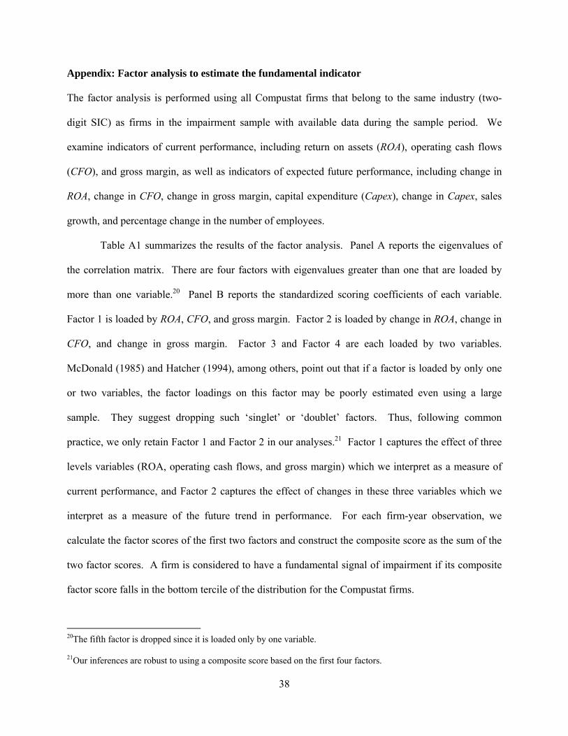
38
Appendix: Factor analysis to estimate the fundamental indicator The factor analysis is performed using all Compustat firms that belong to the same industry (two-
digit SIC) as firms in the impairment sample with available data during the sample period. We
examine indicators of current performance, including return on assets (ROA), operating cash flows
(CFO), and gross margin, as well as indicators of expected future performance, including change in
ROA, change in CFO, change in gross margin, capital expenditure (Capex), change in Capex, sales
growth, and percentage change in the number of employees.
Table A1 summarizes the results of the factor analysis. Panel A reports the eigenvalues of
the correlation matrix. There are four factors with eigenvalues greater than one that are loaded by
more than one variable.20 Panel B reports the standardized scoring coefficients of each variable.
Factor 1 is loaded by ROA, CFO, and gross margin. Factor 2 is loaded by change in ROA, change in
CFO, and change in gross margin. Factor 3 and Factor 4 are each loaded by two variables.
McDonald (1985) and Hatcher (1994), among others, point out that if a factor is loaded by only one
or two variables, the factor loadings on this factor may be poorly estimated even using a large
sample. They suggest dropping such ‘singlet’ or ‘doublet’ factors. Thus, following common
practice, we only retain Factor 1 and Factor 2 in our analyses.21 Factor 1 captures the effect of three
levels variables (ROA, operating cash flows, and gross margin) which we interpret as a measure of
current performance, and Factor 2 captures the effect of changes in these three variables which we
interpret as a measure of the future trend in performance. For each firm-year observation, we
calculate the factor scores of the first two factors and construct the composite score as the sum of the
two factor scores. A firm is considered to have a fundamental signal of impairment if its composite
factor score falls in the bottom tercile of the distribution for the Compustat firms.
20The fifth factor is dropped since it is loaded only by one variable. 21Our inferences are robust to using a composite score based on the first four factors.
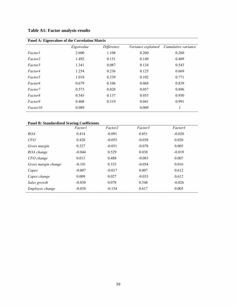
39
Table A1: Factor analysis results Panel A: Eigenvalues of the Correlation Matrix
Eigenvalue Difference Variance explained Cumulative variance
Factor1 2.600 1.108 0.260 0.260
Factor2 1.492 0.151 0.149 0.409
Factor3 1.341 0.087 0.134 0.543
Factor4 1.254 0.236 0.125 0.669
Factor5 1.018 0.339 0.102 0.771
Factor6 0.679 0.106 0.068 0.839
Factor7 0.573 0.028 0.057 0.896
Factor8 0.545 0.137 0.055 0.950
Factor9 0.408 0.319 0.041 0.991
Factor10 0.089 0.009 1
Panel B: Standardized Scoring Coefficients
Factor1 Factor2 Factor3 Factor4
ROA 0.414 -0.091 0.051 -0.020
CFO 0.420 -0.055 -0.038 0.020
Gross margin 0.327 -0.051 -0.078 0.005
ROA change -0.044 0.529 0.038 -0.019
CFO change 0.013 0.488 -0.083 0.007
Gross margin change -0.101 0.333 -0.054 0.016
Capex -0.007 -0.017 0.007 0.612
Capex change 0.009 0.027 -0.033 0.612
Sales growth -0.030 0.078 0.548 -0.026
Employee change -0.038 -0.154 0.617 0.005

40
Table 1: Descriptive statistics of the sample of goodwill impairments Panel A: Distribution of impairment sample by year
Year All goodwill impairments Percentage
2002 215 13.93%
2003 159 10.30%
2004 139 9.01%
2005 160 10.37%
2006 161 10.43%
2007 149 9.66%
2008 473 30.65%
2009 87 5.64%
Total 1543 100% Panel B: Firm characteristics of impairment and control firms This panel reports statistics of the entire impairment sample and its matched control sample. Total Assets represents total assets (in millions) at the beginning of the impairment year. MV is the market value of equity (in millions) at the beginning of the impairment year. ImpairAmt is equal to the after-tax amount of goodwill impairment scaled by beginning-of-the-year market value of equity. ΔROA is change in operating income before goodwill impairment scaled by beginning-of-the-year total assets. M/B is computed as market value of equity at the end of the impairment year over book value of equity before goodwill impairment at the end of the year. Fundamental is the sum of the first two factor scores extracted from a factor analysis of various indicators capturing current and expected future performance, including ROA, change in ROA, operating cash flows to total assets, change in operating cash flows to total assets, gross margin, change in gross margin, sales growth, capital expenditure scaled by total assets, change in capital expenditure, and change in the number of employees. RET is the buy-and-hold market-adjusted returns of the impairment year. Spread is the average daily bid-ask spread in the impairment year. Forecast Dispersion is calculated as the annual average of the quarterly standard-deviation of one-quarter-ahead forecasts issued by analysts for the impairment year, scaled by beginning-of-the-year stock price. T-tests (Wilcoxon tests) are conducted to test the difference in means (distributions) of the impairment and the control samples. *, **, *** indicate the significance of differences at the 10%, 5%, and 1% levels, respectively.
Variable
Impairment Control
Mean Median Mean Median
Total Assets 8478.61 959.52 5762.56** 323.41***
MV 6069.91 607.38 4906.67 326.36***
ImpairAmt 0.05 0.02 - -
ΔROA -0.03 -0.01 -0.01*** -0.01***
M/B 1.87 1.25 2.53*** 1.54***
Fundamental -0.14 0.09 -0.12 0.10
RET -0.11 -0.16 -0.02*** -0.09***
Spread 0.05 0.05 0.05 0.05
Forecast Dispersion 0.01 0.00 0.00*** 0.00***
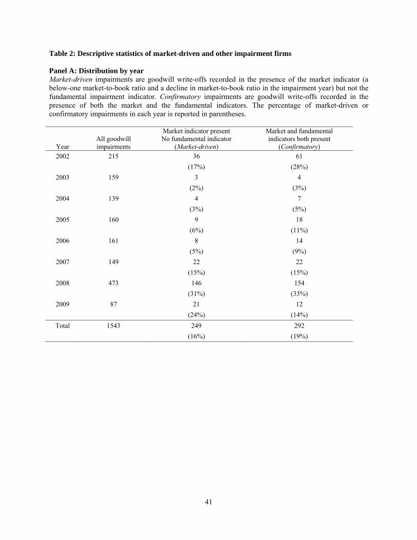
41
Table 2: Descriptive statistics of market-driven and other impairment firms Panel A: Distribution by year Market-driven impairments are goodwill write-offs recorded in the presence of the market indicator (a below-one market-to-book ratio and a decline in market-to-book ratio in the impairment year) but not the fundamental impairment indicator. Confirmatory impairments are goodwill write-offs recorded in the presence of both the market and the fundamental indicators. The percentage of market-driven or confirmatory impairments in each year is reported in parentheses.
Year All goodwill impairments
Market indicator present No fundamental indicator
(Market-driven)
Market and fundamental indicators both present
(Confirmatory)
2002 215 36 61
(17%) (28%)
2003 159 3 4
(2%) (3%)
2004 139 4 7
(3%) (5%)
2005 160 9 18
(6%) (11%)
2006 161 8 14
(5%) (9%)
2007 149 22 22
(15%) (15%)
2008 473 146 154
(31%) (33%)
2009 87 21 12
(24%) (14%)
Total 1543 249 292
(16%) (19%)

42
Panel B: Market-driven impairments vs. other impairments This panel presents statistics of market-driven impairments, all other impairments, and confirmatory impairments separately. All variables are defined in Table 1, Panel B. T-tests (Wilcoxon tests) are conducted to test the difference in means (distributions) of the market-driven impairments and all other impairments or confirmatory impairments. *, **, *** indicate the significance of differences at the 10%, 5%, and 1% levels, respectively.
Variable
Market-driven All others Confirmatory
Mean Median Mean Median Mean Median
Total Assets 8733.34 790.60 8429.40 972.91 3497.59*** 425.13***
MV 3314.35 265.54 6602.28*** 733.98*** 1033.55** 149.36***
ImpairAmt 0.08 0.06 0.05*** 0.01*** 0.10* 0.07**
ΔROA 0.01 -0.01 -0.03*** -0.01*** -0.11*** -0.07***
M/B 0.65 0.65 2.11*** 1.49*** 0.62 0.61
Fundamental 0.43 0.32 -0.25*** -0.03*** -1.08*** -0.75***
RET -0.21 -0.23 -0.09*** -0.15*** -0.36*** -0.33***
Spread 0.06 0.06 0.05*** 0.04*** 0.07** 0.07**
Forecast Dispersion 0.01 0.01 0.01** 0.00*** 0.01 0.00
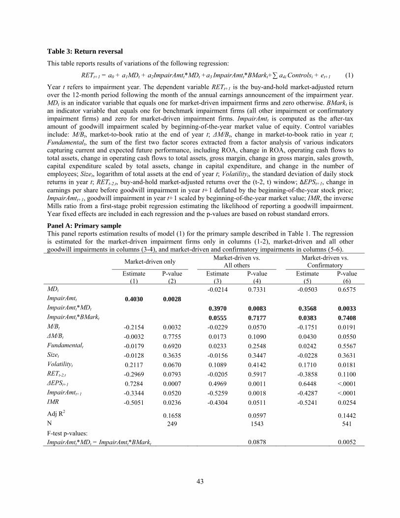
43
Table 3: Return reversal
This table reports results of variations of the following regression:
RETt+1 = a0 + a1MDt + a2ImpairAmtt*MDt +a3 ImpairAmtt*BMarkt+∑ a4i Controlsi + et+1 (1)
Year t refers to impairment year. The dependent variable RETt+1 is the buy-and-hold market-adjusted return over the 12-month period following the month of the annual earnings announcement of the impairment year. MDt is an indicator variable that equals one for market-driven impairment firms and zero otherwise. BMarkt is an indicator variable that equals one for benchmark impairment firms (all other impairment or confirmatory impairment firms) and zero for market-driven impairment firms. ImpairAmtt is computed as the after-tax amount of goodwill impairment scaled by beginning-of-the-year market value of equity. Control variables include: M/Bt, market-to-book ratio at the end of year t; ΔM/Bt, change in market-to-book ratio in year t; Fundamentalt, the sum of the first two factor scores extracted from a factor analysis of various indicators capturing current and expected future performance, including ROA, change in ROA, operating cash flows to total assets, change in operating cash flows to total assets, gross margin, change in gross margin, sales growth, capital expenditure scaled by total assets, change in capital expenditure, and change in the number of employees; Sizet, logarithm of total assets at the end of year t; Volatilityt, the standard deviation of daily stock returns in year t; RETt-2,t, buy-and-hold market-adjusted returns over the (t-2, t) window; ΔEPSt+1, change in earnings per share before goodwill impairment in year t+1 deflated by the beginning-of-the-year stock price; ImpairAmtt+1, goodwill impairment in year t+1 scaled by beginning-of-the-year market value; IMR, the inverse Mills ratio from a first-stage probit regression estimating the likelihood of reporting a goodwill impairment. Year fixed effects are included in each regression and the p-values are based on robust standard errors.
Panel A: Primary sample This panel reports estimation results of model (1) for the primary sample described in Table 1. The regression is estimated for the market-driven impairment firms only in columns (1-2), market-driven and all other goodwill impairments in columns (3-4), and market-driven and confirmatory impairments in columns (5-6).
Market-driven only Market-driven vs.
All others
Market-driven vs. Confirmatory
Estimate (1)
P-value (2)
Estimate (3)
P-value (4)
Estimate (5)
P-value (6)
MDt -0.0214 0.7331 -0.0503 0.6575 ImpairAmtt 0.4030 0.0028 ImpairAmtt*MDt 0.3970 0.0083 0.3568 0.0033 ImpairAmtt*BMarkt 0.0555 0.7177 0.0383 0.7408 M/Bt -0.2154 0.0032 -0.0229 0.0570 -0.1751 0.0191 ΔM/Bt -0.0032 0.7755 0.0173 0.1090 0.0430 0.0550 Fundamentalt -0.0179 0.6920 0.0233 0.2548 0.0242 0.5567 Sizet -0.0128 0.3635 -0.0156 0.3447 -0.0228 0.3631 Volatilityt 0.2117 0.0670 0.1089 0.4142 0.1710 0.0181 RETt-2,t -0.2969 0.0793 -0.0205 0.5917 -0.3858 0.1100 ΔEPSt+1 0.7284 0.0007 0.4969 0.0011 0.6448 <.0001 ImpairAmtt+1 -0.3344 0.0520 -0.5259 0.0018 -0.4287 <.0001 IMR -0.5051 0.0236 -0.4304 0.0511 -0.5241 0.0254
Adj R2 0.1658 0.0597 0.1442 N 249 1543 541
F-test p-values: ImpairAmtt*MDt = ImpairAmtt*BMarkt 0.0878 0.0052

44
Panel B: Sample including delisted firms This panel reports the estimation results of model (1) for the primary sample plus impairment firms delisted in the year subsequent to the impairment. The regression is estimated for the market-driven impairment firms only in columns (1-2), market-driven and all other goodwill impairments in columns (3-4), and market-driven and confirmatory impairments in columns (5-6).
Market-driven only Market-driven vs.
All others
Market-driven vs. Confirmatory
Estimate (1)
P-value (2)
Estimate (3)
P-value (4)
Estimate (5)
P-value (6)
MDt -0.0560 0.2555 -0.0866 0.2889 ImpairAmtt 0.3817 0.0467 ImpairAmtt*MDt 0.3844 0.0304 0.4262 0.0380 ImpairAmtt*BMarkt -0.0677 0.5196 0.0433 0.8286 M/Bt -0.1335 0.3403 -0.0122 0.0362 -0.1030 0.1070 ΔM/Bt 0.0038 0.9533 0.0126 0.2175 0.0443 0.3319 Fundamentalt -0.0050 0.9580 0.0173 0.2746 0.0250 0.5034 Sizet -0.0078 0.7946 -0.0097 0.3308 -0.0277 0.2473 Volatilityt 0.0507 0.7435 0.0965 0.0112 0.0576 0.6055 RETt-2,t -0.2700 0.0321 -0.0065 0.6729 -0.2773 0.0020 ΔEPSt+1 0.6550 0.0123 0.5176 0.0002 0.5717 0.0008 IMR -0.4451 0.2111 -0.2057 0.0759 -0.4247 0.0922 Adj R2 0.1196 0.0323 0.1099 N 270 1910 593
F-test p-values: ImpairAmtt*MDt = ImpairAmtt*BMarkt 0.0292 0.1549

45
Table 4: Market reaction to impairment announcement This table reports the results of the following regression:
3-DRETt =a0+ a1 MDt + a2ImpairAmtt*MDt + a3 ImpairAmtt*BMarkt + a4∆EPSt+ a5IMR+et (2)
The dependent variable, 3-DRETt, is computed as the 3-day market-adjusted returns around the earnings announcement of the impairment quarter. ImpairAmtt is the amount of goodwill impairment in quarter t scaled by beginning-of-the-quarter market value. ∆EPSt is the seasonally-adjusted change in earnings per share (before goodwill impairment) of quarter t scaled by beginning-of-the-quarter stock price. Year fixed effects are included in each regression and the p-values are computed based on robust standard errors.
Panel A: Primary sample This panel reports the estimation results of model (2) for the primary sample described in Table 1. The regression is estimated for the market-driven impairment firms only in columns (1-2), market-driven and all other goodwill impairments in columns (3-4), and market-driven and confirmatory impairments in columns (5-6).
Market-driven only Market-driven vs.
All others
Market-driven vs. Confirmatory
Estimate (1)
P-value (2)
Estimate (3)
P-value (4)
Estimate (5)
P-value (6)
MDt 0.0196 0.0798 0.0373 0.0003 ImpairAmtt -0.0532 0.0048 ImpairAmtt*MDt -0.0486 0.0034 -0.0503 0.0048 ImpairAmtt*BMarkt -0.0650 0.0017 -0.0382 0.0652 ΔEPSt 0.0002 0.7158 0.0004 0.0670 0.0002 0.5004 IMR 0.0213 0.3214 0.0035 0.7957 0.0437 0.0248 Adj R2 0.0194 0.0186 0.0357 N 266 1653 571
F-test p-values: ImpairAmtt*MDt = ImpairAmtt*BMarkt
0.1498 0.5280

46
Panel B: Sample including delisted firms This panel reports the estimation results of model (2) for the primary sample plus impairment firms delisted in the year subsequent to the impairment. The regression is estimated for the market-driven impairment firms only in columns (1-2), market-driven and all other goodwill impairments in columns (3-4), and market-driven and confirmatory impairments in columns (5-6).
Market-driven only Market-driven vs.
All others
Market-driven vs. Confirmatory
Estimate (1)
P-value (2)
Estimate (3)
P-value (4)
Estimate (5)
P-value (6)
MDt 0.0181 0.1260 0.0304 0.0093 ImpairAmtt -0.0529 0.0196 ImpairAmtt*MDt -0.0481 0.0086 -0.0488 0.0145 ImpairAmtt*BMarkt -0.0476 0.0170 -0.0556 0.0038 ΔEPSt 0.0002 0.6672 0.0005 0.0321 0.0004 0.2862 IMR 0.0274 0.2862 0.0089 0.5654 0.0395 0.0273 Adj R2 0.0267 0.0139 0.0367 N 288 2035 624
F-test p-values: ImpairAmtt*MDt = ImpairAmtt*BMarkt
0.9866 0.6872

47
Table 5: Timing of return reversal This table reports the results on the timing of return reversal. The following regression is estimated:
BHRETt+1,k= a0 + a1 ImpairAmtt + ∑ a2i Controlsi + et+1
The dependent variable, BHRETt+1,k, is computed as buy-and-hold market-adjusted returns from the month following the earnings announcement of impairment year t up to the end of the earnings announcement month of the kth quarter of year t+1. Control variables are the same as in Table 3 except that, in this regression, ΔEPSt+1 and ImpairAmtt+1 are computed as cumulative earnings and impairment from the month following the earnings announcement of impairment year t up to the end of the earnings announcement month of the kth quarter. The regression is estimated for market-driven, all other, and confirmatory impairment firms separately in columns (1-2), (3-4), and (5-6), respectively. Year fixed effects are included in each regression and the p-values are based on robust standard errors. For brevity, only the coefficient estimates and p-values (in parentheses) on ImpairAmtt (a1) are reported.
Dependent Variable Market-driven
(1) All others
(2) Confirmatory
(3)
BHRETt+1,1 -0.0375 -0.0729 -0.0171
(0.7288) (0.4463) (0.8640)
BHRETt+1,2 -0.0833 -0.1347 -0.4375
(0.7898) (0.3343) (0.0875)
BHRETt+1,3 0.3971 0.0686 -0.3664
(0.3069) (0.7146) (0.4184)
BHRETt+1,4 0.4030 0.0824 -0.0279
(0.0028) (0.5665) (0.9111)

48
Table 6: Information asymmetry This table reports the test results of H2 on changes in information asymmetry. Panel A: Bid-ask spread as a measure of information asymmetry This table reports the estimation results of variations of the following regression:
ΔSpreadt+1 = a0 + a1 MDt + a2Controlt + a4 Controlt*MD t + a3ImpairAmtt + a5 ImpairAmtt*MDt +
∑ a6i Control Variablei + et+1 (3)
Year t refers to the impairment year. The dependent variable ΔSpreadt+1 is the difference in the bid-ask spread between the year subsequent to the impairment (year t+1) and the year before the impairment (year t-1). Control is an indicator variable equal to one for matched control non-impairment firms and zero for impairment firms. Among control variables, Pricet+1, equals the logarithm of stock price at the end of year t+1. Deptht+1 is computed as the logarithm of the number of outstanding common shares at the end of year t+1. Volatilityt (Volatilityt+1) is the standard deviation of daily returns over the 250-day period before the earnings announcement of year t (year t+1). All other variables are defined in Table 3. The regression is estimated for market-driven and matched control firms in columns (1-2), the entire goodwill impairment sample and matched control firms in columns (3-4), and market-driven and confirmatory impairment firms and their matched control firms in columns (5-6). Year fixed effects are included in each regression and the p-values are based on robust standard errors.
Market-driven only Market-driven vs.
All others
Market-driven vs. Confirmatory
Estimate (1)
P-value (2)
Estimate (3)
P-value (4)
Estimate (5)
P-value (6)
MDt 0.0005 0.2061 0.0017 0.1130 Controlt 0.0000 0.9748 -0.0004 0.6545 0.0003 0.8512 Control*MDt -0.0006 0.5940 -0.0020 0.1797 ImpairAmtt 0.0107 0.0085 0.0017 0.4345 -0.0033 0.2565 ImpairAmtt*MDt 0.0104 0.0113 0.0128 0.0051 M/Bt 0.0008 0.6735 -0.0002 0.0211 0.0018 0.2276 ΔM/Bt -0.0016 0.0253 0.0000 0.9439 -0.0004 0.4474 Fundamentalt -0.0026 0.0259 0.0001 0.6883 -0.0002 0.6363 Sizet 0.0003 0.6185 0.0001 0.5999 0.0009 0.0862 Pricet+1 -0.0010 0.1929 -0.0016 <.0001 -0.0026 <.0001 Deptht+1 -0.0008 0.0509 -0.0008 <.0001 -0.0009 0.0010 Volatilityt 0.0356 <.0001 0.0323 <.0001 0.0369 <.0001 Volatilityt+1 -0.0312 <.0001 -0.0347 <.0001 -0.0334 <.0001 ImpairAmtt+1 -0.0001 0.9775 0.0064 0.0399 -0.0001 0.9879 IMR -0.0075 0.0899 -0.0052 0.0053 -0.0059 0.0882
Adj R2 0.8890 0.8485 0.8842 N 496 3086 1082

49
Panel B: Analyst forecast dispersion as a measure of information asymmetry This table reports the estimation results of variations of the following regression:
ΔDispersiont+1 = a0 + a1 MDt + a2Controlt + a3 Controlt*MDt + a4ImpairAmtt + a5 ImpairAmtt *MDt + ∑ a6i Control Variablei + et+1 (4)
Year t refers to the impairment year. The dependent variable ΔDispersiont+1 is equal to the analyst forecast dispersion of the year subsequent to the impairment year (year t+1) minus that of the year before the impairment (year t-1). Analyst forecast dispersion is computed as the annual average standard deviation of one-quarter-ahead forecasts issued by analysts, scaled by beginning-of-the-year stock price. Among control variables, Losst+1, is equal to one if earnings of year t+1 is negative and zero otherwise. Std_ROEt-5,t is computed as the standard deviation of annual earnings over the past five years (year t-5 to year t). LogMVt is the logarithm of market value of equity at the end of year t. NForecast is the logarithm of the number of one-quarter-ahead forecasts in year t+1. All other variables are defined in Table 3. The regression is estimated for the market-driven impairment firms and their control firms in columns (1-2), the market-driven and all other goodwill impairment firms and their matched control firms in column (3-4), and the market-driven and confirmatory impairment firms and their matched control firms in column (5-6). Year fixed effects are included in each regression and the p-values are based on robust standard errors.
Market-driven only Market-driven vs.
All others
Market-driven vs. Confirmatory
Estimate
(1) P-value
(2) Estimate
(3) P-value
(4) Estimate
(5) P-value
(6) MDt 0.0009 0.1361 0.0070 0.1027 Controlt -0.0005 0.8055 -0.0010 0.5745 -0.0011 0.7668 Controlt*MDt -0.0023 0.2703 -0.0091 0.0873 ImpairAmtt 0.0153 0.0906 -0.0194 0.0274 -0.0530 0.0339 ImpairAmtt*MDt 0.0333 0.0006 0.0529 0.0161 M/Bt 0.0054 0.0842 0.0000 0.4566 0.0059 0.1420 ΔM/Bt 0.0000 0.9788 0.0000 0.6735 -0.0006 0.2403 Fundamentalt -0.0058 0.0069 0.0004 0.4050 0.0031 0.1908 Losst+1 0.0010 0.6423 0.0011 0.3114 -0.0005 0.8566 Std_ROEt-5,t -0.0006 0.6895 0.0007 0.3145 0.0025 0.2580 LogMVt 0.0000 0.9976 0.0002 0.5343 0.0000 0.9813 NForecastt+1 -0.0003 0.8054 0.0001 0.8631 -0.0002 0.8213 ImpairAmtt+1 0.0047 0.7131 0.0158 0.0183 0.0008 0.9509 IMR 0.0063 0.4351 0.0017 0.6403 -0.0040 0.6229
Adj R2 0.2186 0.0796 0.1613 N 172 1196 334

50
Table 7: Stock repurchases This table reports the test results of H3 on share repurchases. Panel A: Regression analysis – decision to repurchase This table reports the estimation results of the following logistic regression:
Repurchaset+1 = a0 + a1 MDt + a2Controlt + a3 Controlt*MDt + a4 ImpairAmtt + a5 ImpairAmtt *MDt +
∑ a6i Control Variablei + et+1 (5)
Year t refers to the impairment year. The dependent variable Repurchaset+1 is a dummy variable equal to one if a firm repurchases its stock in year t+1 and zero otherwise. Control is an indicator variable equal to one for matched control non-impairment firms and zero for impairment firms. Among control variables, Casht is the cash balance scaled by market value of equity at the end of year t. Payoutt+1 is computed as dividend over net income of year t+1. Leveraget is industry-average-adjusted leverage ratio, where the leverage ratio is defined as total debt over the sum of market value of equity and total debt. OptionExercisable (OptionExercised) is the number of exercisable (exercised) options in year t+1 scaled by the number of common shares outstanding at the beginning of the year. All other variables are defined in Table 3. Year fixed effects are included in the regressions and the p-values are based on robust standard errors.
Market-driven only Market-driven vs.
All others
Market-driven vs. Confirmatory
Estimate
(1) P-value
(2) Estimate
(3) P-value
(4) Estimate
(5) P-value
(6) MD 0.4192 <.0001 0.2997 0.0393 Control 0.2623 0.5115 0.2985 0.4298 0.4312 <.0001 Control*MD -0.6883 0.1603 -0.5372 0.2215 ImpairAmtt 1.9403 0.0302 -0.6617 0.3013 -0.2273 0.7008 ImpairAmtt*MDt 1.8272 0.0014 1.9556 0.0030 M/Bt 0.0010 0.7180 -0.0005 0.1456 0.0022 0.9797 ΔM/Bt -0.2426 0.1422 -0.0014 0.5102 -0.0412 0.7501 Fundamentalt -0.7273 0.0788 0.2948 <.0001 0.0658 0.6491 Casht -1.0681 0.2836 0.3027 0.0982 -0.1713 0.6731 Payoutt+1 -0.0098 0.8656 -0.0166 <.0001 -0.0165 <.0001 Leveraget -4.1629 0.0004 -2.1282 0.0001 -3.2244 0.0001 RETt+1 -0.4346 <.0001 -0.2322 0.0004 -0.2961 <.0001 OptionExercisablet+1 1.9446 0.6650 2.3380 0.0767 -0.6079 0.8115 OptionExercisedt+1 6.7403 0.6171 19.8163 <.0001 54.1798 <.0001 LagRepurchase 2.3626 <.0001 2.3840 <.0001 1.9881 <.0001 IMR -1.2989 0.2859 -1.9517 <.0001 -1.7055 <.0001 Chi-Square stat 268.66 1394.77 520.10 N 498 3086 1082

51
Panel B: Regression analysis – dollar amount of repurchase This table reports the estimation results of the following Tobit regression: Repurchaset+1 = a0 + a1 MDt + a2Controlt + a3Controlt*MDt + a4ImpairAmtt + a5 ImpairAmtt*MDt + ∑ a5i Control Variablei + et+1 (5) The dependent variable Repurchaset+1 is equal to the dollar amount of stock repurchases during year t+1. All other variables are defined in Panel A and Table 3. Year fixed effects are included in the regressions and the p-values are based on robust standard errors.
Market-driven only Market-driven vs.
All others
Market-driven vs. Confirmatory
Estimate (1)
P-value (2)
Estimate (3)
P-value (4)
Estimate (5)
P-value (6)
MD 0.0089 0.0000 0.0080 0.1680 Control 0.0067 0.1730 0.0031 0.5360 -0.0002 0.9810 Control*MD -0.0183 0.0020 -0.0175 0.0220 ImpairAmtt 0.0253 0.0680 -0.0195 0.0660 -0.0123 0.4080 ImpairAmtt*MDt 0.0418 0.0440 0.0447 0.0510 M/Bt 0.0000 0.0080 0.0000 0.2240 -0.0005 0.8580 ΔM/Bt -0.0043 0.0420 0.0000 0.1700 -0.0021 0.2000 Fundamentalt 0.0003 0.9370 0.0041 0.0040 0.0066 0.0130 Casht -0.0298 0.0340 0.0069 0.3020 0.0118 0.3650 Payoutt+1 -0.0012 0.0130 -0.0001 0.3210 -0.0001 0.4210 Leveraget -0.0564 0.0000 -0.0430 0.0000 -0.0516 0.0000 RETt+1 -0.0014 0.1830 -0.0010 0.5590 -0.0021 0.3260 OptionExercisablet+1 0.1391 0.0590 0.0881 0.0010 0.0590 0.1450 OptionExercisedt+1 0.3080 0.2770 0.3027 0.0000 0.6861 0.0040 LagRepurchase -0.0126 0.8210 0.1647 0.0000 0.0252 0.5760 IMR -0.0353 0.2000 -0.0395 0.0000 -0.0440 0.0010 Chi-Square stat 218.34 1196.67 345.32 N 490 3080 1076

52
Table 8: Impairments during the financial crisis This table reports the estimated coefficient of interest in the following regressions. In all regressions, the benchmark impairment sample is all impairment firms other than market-driven impairment firms. Year fixed effects are included in each regression and the p-values are based on robust standard errors. In columns (1-4), the following regressions are estimated for all impairments during the financial crisis period and the rest of the impairment sample separately, respectively:
RETt+1 = a0 + a1MDt + a2ImpairAmtt*MDt +a3 ImpairAmtt*BMarkt+∑ a4i Controlsi + et+1 (1)
3-DRETt =a0+ a1 MDt + a2ImpairAmtt*MDt + a3 ImpairAmtt*BMarkt + a4∆EPSt+ a5IMR+et (2)
ΔSpreadt+1 = a0 + a1 MDt + a2Controlt + a4 Controlt*MD t + a3ImpairAmtt + a5 ImpairAmtt*MDt +
∑ a6i Control Variablei + et+1 (3)
Repurchaset+1 = a0 + a1 MDt + a2Controlt + a3 Controlt*MDt + a4 ImpairAmtt + a5 ImpairAmtt *MDt +
∑ a6i Control Variablei + et+1 (5)
The coefficient on ImpairAmtt*MDt is reported in each column with the p-value in parentheses. All other variables are defined in Tables 3-7. Return
reversal
(1)
H1: Market reaction
(2)
H2: Change in bid-ask spread
(3)
H3: Stock repurchase
(4)
Financial crisis period 0.6681
(0.0322)
-0.0437
(0.0818)
0.0096
(0.0496)
2.1875
(0.0487)
Non-financial crisis period 0.6327
(0.0906)
-0.0665
(0.0697)
0.0177
(0.0004)
2.5620
(0.0707)