arX

iv:1

609.

0883

8v1

[ast

ro-p

h.G

A]

28 S

ep 2

016

Mon. Not. R. Astron. Soc.000, 1–13 (2016) Printed 6 August 2018 (MN LATEX style file v2.2)

Constraining the Galactic structure parameters with theXSTPS-GAC and SDSS photometric surveys

B.-Q. Chen,1‹: X.-W. Liu,1,2‹ H.-B. Yuan,3 A.C. Robin,4 Y. Huang,1: M.-S. Xiang,5:

C. Wang,1 J.-J. Ren,1,5 Z.-J. Tian,1: H.-W. Zhang11Department of Astronomy, Peking University, Beijing 100871, P. R. China2Kavli Institute for Astronomy and Astrophysics, Peking University, Beijing 100871, P. R. China3Department of Astronomy, Beijing Normal University, Beijing 100875, P. R. China4Institut Utinam, CNRS UMR6213, OSU THETA, Universite de Bourgogne-Franche-Comte, Observatoire de Besancon, 25010 Besancon, France5National Astronomy Observatories, Chinese Academy of Sciences, Beijing 100012, P. R. China

Accepted ???. Received ???; in original form ???

ABSTRACTPhotometric data from the Xuyi Schmidt Telescope Photometric Survey of the Galactic Anti-centre (XSTPS-GAC) and the Sloan Digital Sky Survey (SDSS) are used to derive the globalstructure parameters of the smooth components of the Milky Way. The data, which covernearly 11,000 deg2 sky area and the full range of Galactic latitude, allow us to construct aglobally representative Galactic model. The number density distribution of Galactic halo starsis fitted with an oblate spheroid that decays by power law. Thebest-fit yields an axis ratio anda power law indexκ “ 0.65 andp “ 2.79, respectively. Ther-band differential star countsof three dwarf samples are then fitted with a Galactic model. The best-fit model yielded bya Markov Chain Monte Carlo analysis has thin and thick disk scale heights and lengths ofH1 “ 322 pc andL1 “2343pc,H2 “794 pc andL2 “3638 pc, a local thick-to-thin diskdensity ratio off2 “11 per cent, and a local density ratio of the oblate halo to thethin diskof fh “0.16per cent. The measured star count distribution, which is in good agreement withthe above model for most of the sky area, shows a number of statistically significant largescale overdensities, including some of the previously known substructures, such as the Virgooverdensity and the so-called “north near structure”, and anew feature between 150˝

ă l ă

240˝ and´15˝ă b ă ´5˝, at an estimated distance between 1.0 and 1.5 kpc. The Galactic

North-South asymmetry in the anticentre is even stronger than previously thought.

Key words: Galaxy: disk - Galaxy: structure - Galaxy: fundamental parameters

1 INTRODUCTION

One of the fundamental tasks of the Galactic studies is to esti-mate the structure parameters of the major structure components.Bahcall & Soneira (1980) fit the observations with two structurecomponents, namely a disk and a halo. Gilmore & Reid (1983)introduce a third component, namely a thick disk, confirmed inthe earliest Besancon Galaxy Model Creze & Robin (1983). Sincethen, various methods and observations have been adopted toes-timate parameters of the thin and thick disks and of the halo ofour Galaxy. As the quantity and quality of data available con-tinue to improve over the years, the model parameters derived havebecome more precise, numerically. Ironically, those numericallymore precise results do not converge (see Table 1 of Chang et al.2011, Table 2 of Lopez-Corredoira & Molgo 2014 and Sect. 5 and6 of Bland-Hawthorn & Gerhard 2016 for a review). The scatters

‹ E-mail: bchen@pku.edu.cn (BQC); x.liu@pku.edu.cn (XWL).: LAMOST Fellow.

in density law parameters, such as scale lengths, scale heightsand local densities of these Galactic components, as reported inthe literature, are rather large. At least parts of the discrepan-cies are caused by degeneracy of model parameters, which inturn, can be traced back to the different data sets adopted in theanalyses. Those differing data sets either probe different sky ar-eas (Bilir et al. 2006a; Du et al. 2006; Cabrera-Lavers et al.2007;Ak et al. 2007; Yaz & Karaali 2010; Yaz Gokce et al. 2015), are ofdifferent completeness magnitudes and therefore refer to differentlimiting distances (Karaali et al. 2007), or of consist of stars of dif-ferent populations of different absolute magnitudes (Karaali et al.2004; Bilir et al. 2006b; Juric et al. 2008; Jia et al. 2014).It shouldbe noted that the analysis of Bovy et al. (2012), using the SEGUEspectroscopic survey, has given a new insight on the thin andthickdisk structural parameters. This analysis provides estimate of theirscale height and scale height as a function of metallicity and alphaabundance ratio. However, it relies on incomplete data (since it isspectroscopic) with relatively low range of Galactocentric radius asfor the thin disk is concerned.

c© 2016 RAS

2 B.Q. Chen et al.

A wider and deeper sample than those employed hitherto mayhelp break the degeneracy inherent in a multi-parameter analysisand yield a globally representative Galactic model. A single or afew fields are insufficient to break the degeneracy. The resultedbest-fit parameters, while sufficient for the description of the linesof sight observed, may be unrepresentative of the entire Galaxy.For the latter purpose, systematic surveys of deep limitingmagni-tude of all or a wide sky area, such as the Two Micron All SkySurvey (2MASS; Skrutskie et al. 2006), the Sloan Digital SkySur-vey (SDSS; York et al. 2000), the Panoramic Survey Telescope&Rapid Response System (Pan-Starrs; Kaiser et al. 2002) and theGAIA mission (Perryman et al. 2001), are always preferred.

Several authors have studied the Galactic structurewith 2MASS data at low (Lopez-Corredoira et al. 2002;Yaz Gokce et al. 2015) or high latitudes (Cabrera-Lavers et al.2005, 2007; Chang et al. 2011). Polido et al. (2013) uses themodel from Ortiz & Lepine (1993) and rederive the parametersof this model based on the 2MASS star counts over the wholesky area. However, the survey depth of 2MASS is not quiteenough to reach the outer disk and the halo. The survey depthof SDSS is much deeper than that of the 2MASS. Many authors(e.g. Chen et al. 2001; Bilir et al. 2006a, 2008; Jia et al. 2014;Lopez-Corredoira & Molgo 2014) have previously used the SDSSdata to constrain the Galactic parameters. Those authors have onlymade use of a portion of the surveyed fields, at intermediate orhigh Galactic latitudes. Juric et al. (2008) obtain Galactic modelparameters from the stellar number density distribution of48million stars detected by the SDSS that sample distances from100 pc to 20 kpc and cover 6500 deg2 of sky. Their results areamongst those mostly quoted. However, in their analysis, theyhave avoided the Galactic plane. So the constraints of theirresultson the disks, especially the thin disk, are weak. In their analysis,Juric et al. (2008) have also adopted photometric parallaxes as-suming that all stars of the same colour have the same metallicity.Clearly, (disk) stars in different parts of the Galaxy have quitedifferent (Ivezic et al. 2008; Xiang et al. 2015; Huang et al. 2015)metallicities, and these variations in metallicities may well lead tobiases in the model parameters derived.

In order to provide a quality input catalog for the LAM-OST Spectroscopic Survey of the Galactic Anticentre (LSS-GAC;Liu et al. 2014, 2015; Yuan et al. 2015b), a multi-band CCDphotometric survey of the Galactic Anticentre with the Xuyi1.04/1.20m Schmidt Telescope (XSTPS-GAC; Zhang et al. 2013,2014; Liu et al. 2014) has been carried out. The XSTPS-GAC pho-tometric catalog contains more than 100 million stars in thedirec-tion of Galactic anticentre (GAC). It provides an excellentdata setto study the Galactic disk, its structures and substructures. In thispaper, we take the effort to constrain the Galactic model param-eters by combining photometric data from the XSTPS-GAC andSDSS surveys. This is the third paper of a series on the Milky Waystudy based on the XSTPS-GAC data. In Chen et al. (2014), wepresent a three dimensional extinction map inr band. The map hasa spatial angular resolution, depending on latitude, between 3 and9 arcmin and covers the entire XSTPS-GAC survey area of over6,000 deg2 for Galactic longitude 140ă l ă220 deg and latitude 40ă b ă40 deg. In Chen et al. (2015), we investigate the correlationbetween the extinction and the HI and CO emission at intermedi-ate and high Galactic latitudes (|b| ą 10˝) within the footprint ofthe XSTPS-GAC, on small and large scales. In the current workweare interested in the global, smooth structure of the Galaxy.

For the Galactic structure, in addition to the global,smooth major components, many more (sub-)structures have

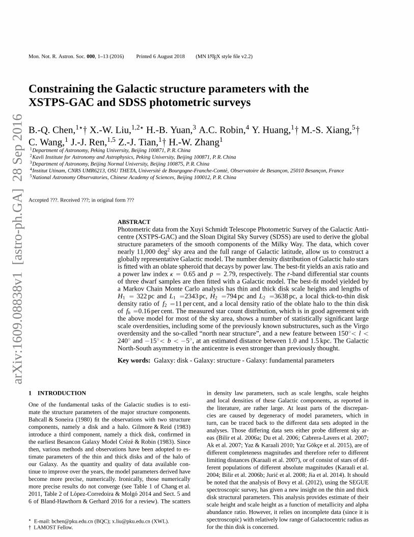
Table 1.Data sets.

area field size Nfields r ranges(deg2) (degˆ deg) (mag)

XSTPS-GAC „3392 2.5 2.5 574 12–18XSTPS-M31/M33 „588 2.5 2.5 108 12–18SDSS „6871 3.0 3.0 1592 15–21

been discovered, including the inner bars near the Galacticcentre (Alves 2000; Hammersley et al. 2000; van Loon et al.2003; Nishiyama et al. 2005; Cabrera-Lavers et al. 2008;Robin et al. 2012), flares and warps of the (outer) disk(Lopez-Corredoira et al. 2002; Robin et al. 2003; Momany etal.2006; Reyle et al. 2009; Lopez-Corredoira & Molgo 2014),andvarious overdensities in the halo and the outer disk, such asthe Sagittarius Stream (Majewski et al. 2003), the Triangulum-Andromeda (Rocha-Pinto et al. 2004; Majewski et al. 2004)and Virgo (Juric et al. 2008) overdensities, the Monocerosring (Newberg et al. 2002; Rocha-Pinto et al. 2003) and theAnti-Center Stream (Rocha-Pinto et al. 2003; Crane et al. 2003;Frinchaboy et al. 2004). They show the complexity of the MilkyWay. Recently, Widrow et al. (2012) and Yanny & Gardner (2013)have found evidence for a significant Galactic North-Southasymmetry in the stellar number density distribution, exhibitingsome wavelike perturbations that seem to be intrinsic to thedisk. Xu et al. (2015) show that in the anticentre regions thereis an oscillating asymmetry in the main-sequence star counts oneither sides of the Galactic plane, in support of the prediction ofIbata et al. (2003). The asymmetry oscillates in the sense that thereare more stars in the north, then in the south, then back in thenorth, and then back in the south at distances of about 2, 4 – 6,8 –10 and 12 – 16 kpc from the Sun, respectively.

The paper is structured as follows. The data are introducedin Section 2. We describe our model and the analysis method inSection 3. Section 4 presents the results and discussions. In Sec-tion 5 we discuss the large scale excess/deficiency of star countsthat reflect the substructures in the halo and disk. Finally we give asummary in Section 6.

2 DATA

2.1 The XSTPS-GAC Data

The XSTPS-GAC started collecting data in the fall of 2009 andcompleted in the spring of 2011. It was carried out in order toprovide input catalogue for the LSS-GAC. The survey was per-formed in the SDSSg, r and i bands using the Xuyi 1.04/1.20 mSchmidt Telescope equipped with a 4kˆ4k CCD camera, operatedby the Near Earth Objects Research Group of the Purple Moun-tain Observatory. The CCD offers a field of view (FoV) of 1.94˝ˆ1.94˝, with a pixel scale of 1.705 arcsec. In total, the XSTPS-GACarchives approximately 100 million stars down to a limitingmag-nitude of about 19 inr band („ 10σ) with an astrometric accuracyabout 0.1 arcsec and a global photometric accuracy of about 2%(Liu et al. 2014). The total survey area of XSTPS-GAC is closeto7,000 deg2, covering an area of„ 5,400 deg2 centered on the GAC,from RA „ 3 to 9 h and Dec„ ´10˝to `60˝, plus an extensionof about 900 deg2 to the M31/M33 area and the bridging fields con-necting the two areas.

c© 2016 RAS, MNRAS000, 1–13

The structure of MW 3

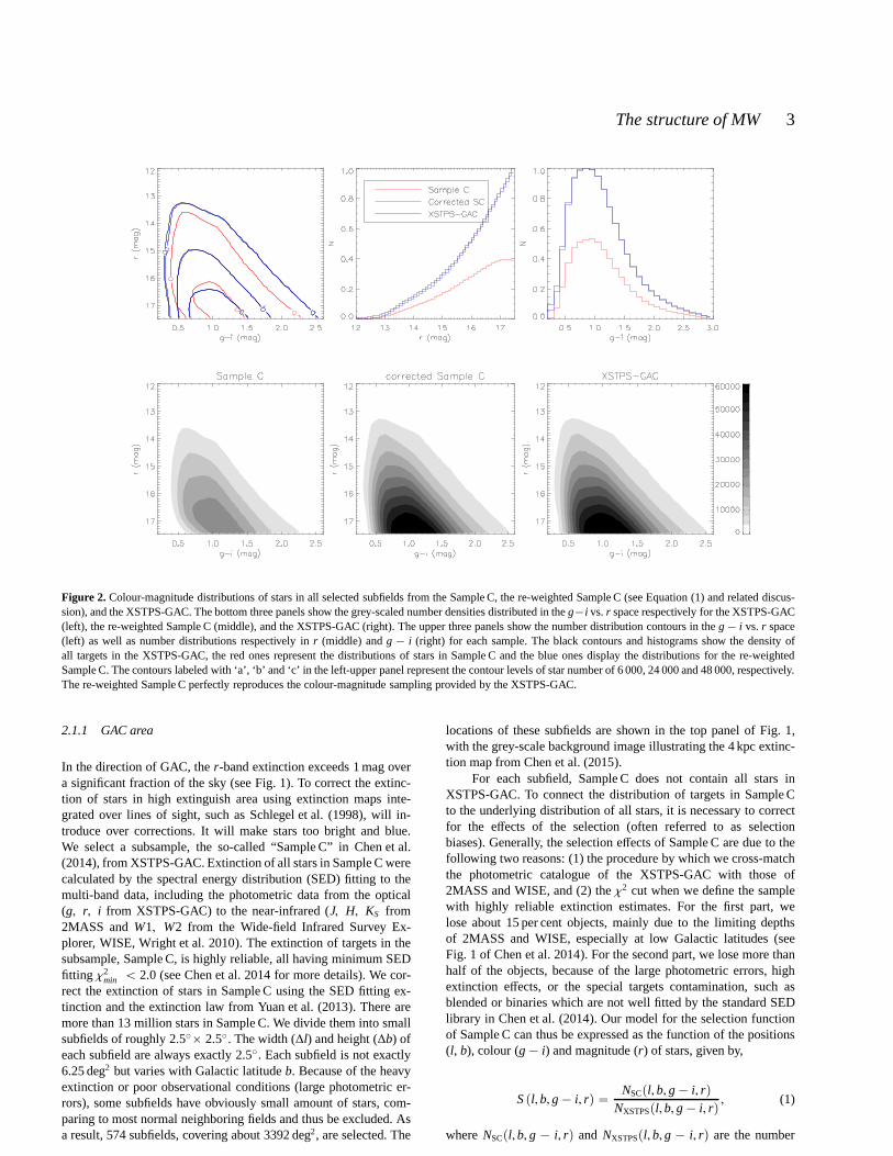
Figure 2. Colour-magnitude distributions of stars in all selected subfields from the Sample C, the re-weighted Sample C (see Equation (1) and related discus-sion), and the XSTPS-GAC. The bottom three panels show the grey-scaled number densities distributed in theg´i vs.r space respectively for the XSTPS-GAC(left), the re-weighted Sample C (middle), and the XSTPS-GAC (right). The upper three panels show the number distribution contours in theg ´ i vs. r space(left) as well as number distributions respectively inr (middle) andg ´ i (right) for each sample. The black contours and histograms show the density ofall targets in the XSTPS-GAC, the red ones represent the distributions of stars in Sample C and the blue ones display the distributions for the re-weightedSample C. The contours labeled with ‘a’, ‘b’ and ‘c’ in the left-upper panel represent the contour levels of star number of6 000, 24 000 and 48 000, respectively.The re-weighted Sample C perfectly reproduces the colour-magnitude sampling provided by the XSTPS-GAC.

2.1.1 GAC area

In the direction of GAC, ther-band extinction exceeds 1 mag overa significant fraction of the sky (see Fig. 1). To correct the extinc-tion of stars in high extinguish area using extinction maps inte-grated over lines of sight, such as Schlegel et al. (1998), will in-troduce over corrections. It will make stars too bright and blue.We select a subsample, the so-called “Sample C” in Chen et al.(2014), from XSTPS-GAC. Extinction of all stars in Sample C werecalculated by the spectral energy distribution (SED) fitting to themulti-band data, including the photometric data from the optical(g, r, i from XSTPS-GAC) to the near-infrared (J, H, KS from2MASS andW1, W2 from the Wide-field Infrared Survey Ex-plorer, WISE, Wright et al. 2010). The extinction of targetsin thesubsample, Sample C, is highly reliable, all having minimumSEDfitting χ2

min ă 2.0 (see Chen et al. 2014 for more details). We cor-rect the extinction of stars in Sample C using the SED fitting ex-tinction and the extinction law from Yuan et al. (2013). There aremore than 13 million stars in Sample C. We divide them into smallsubfields of roughly 2.5˝ˆ 2.5˝. The width (∆l) and height (∆b) ofeach subfield are always exactly 2.5˝. Each subfield is not exactly6.25 deg2 but varies with Galactic latitudeb. Because of the heavyextinction or poor observational conditions (large photometric er-rors), some subfields have obviously small amount of stars, com-paring to most normal neighboring fields and thus be excluded. Asa result, 574 subfields, covering about 3392 deg2, are selected. The

locations of these subfields are shown in the top panel of Fig.1,with the grey-scale background image illustrating the 4 kpcextinc-tion map from Chen et al. (2015).

For each subfield, Sample C does not contain all stars inXSTPS-GAC. To connect the distribution of targets in SampleCto the underlying distribution of all stars, it is necessaryto correctfor the effects of the selection (often referred to as selectionbiases). Generally, the selection effects of Sample C are due to thefollowing two reasons: (1) the procedure by which we cross-matchthe photometric catalogue of the XSTPS-GAC with those of2MASS and WISE, and (2) theχ2 cut when we define the samplewith highly reliable extinction estimates. For the first part, welose about 15 per cent objects, mainly due to the limiting depthsof 2MASS and WISE, especially at low Galactic latitudes (seeFig. 1 of Chen et al. 2014). For the second part, we lose more thanhalf of the objects, because of the large photometric errors, highextinction effects, or the special targets contamination, such asblended or binaries which are not well fitted by the standard SEDlibrary in Chen et al. (2014). Our model for the selection functionof Sample C can thus be expressed as the function of the positions(l, b), colour (g ´ i) and magnitude (r) of stars, given by,

Spl,b,g ´ i, rq “NSCpl,b, g ´ i, rq

NXSTPSpl,b, g ´ i, rq, (1)

whereNSCpl,b, g ´ i, rq and NXSTPSpl,b,g ´ i, rq are the number

c© 2016 RAS, MNRAS000, 1–13

4 B.Q. Chen et al.

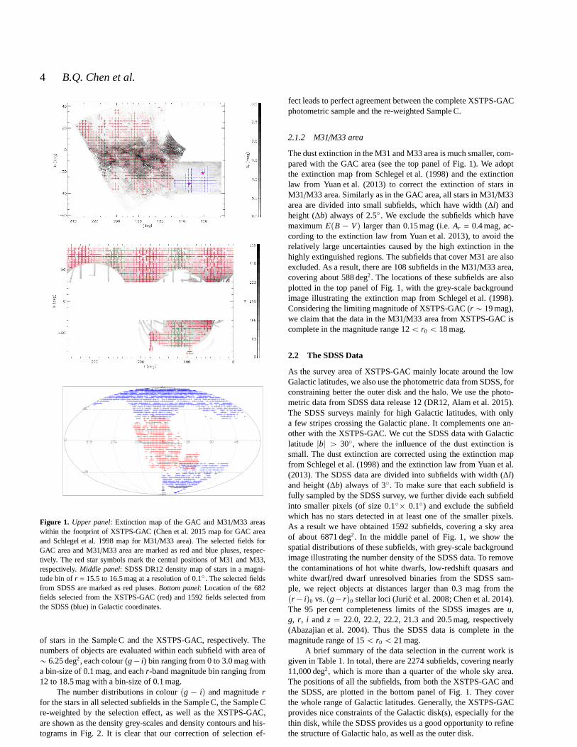
Figure 1. Upper panel: Extinction map of the GAC and M31/M33 areaswithin the footprint of XSTPS-GAC (Chen et al. 2015 map for GAC areaand Schlegel et al. 1998 map for M31/M33 area). The selected fields forGAC area and M31/M33 area are marked as red and blue pluses, respec-tively. The red star symbols mark the central positions of M31 and M33,respectively.Middle panel: SDSS DR12 density map of stars in a magni-tude bin ofr = 15.5 to 16.5 mag at a resolution of 0.1˝. The selected fieldsfrom SDSS are marked as red pluses.Bottom panel: Location of the 682fields selected from the XSTPS-GAC (red) and 1592 fields selected fromthe SDSS (blue) in Galactic coordinates.

of stars in the Sample C and the XSTPS-GAC, respectively. Thenumbers of objects are evaluated within each subfield with area of„ 6.25 deg2, each colour (g´ i) bin ranging from 0 to 3.0 mag witha bin-size of 0.1 mag, and eachr-band magnitude bin ranging from12 to 18.5 mag with a bin-size of 0.1 mag.

The number distributions in colourpg ´ iq and magnituderfor the stars in all selected subfields in the Sample C, the Sample Cre-weighted by the selection effect, as well as the XSTPS-GAC,are shown as the density grey-scales and density contours and his-tograms in Fig. 2. It is clear that our correction of selection ef-

fect leads to perfect agreement between the complete XSTPS-GACphotometric sample and the re-weighted Sample C.

2.1.2 M31/M33 area

The dust extinction in the M31 and M33 area is much smaller, com-pared with the GAC area (see the top panel of Fig. 1). We adoptthe extinction map from Schlegel et al. (1998) and the extinctionlaw from Yuan et al. (2013) to correct the extinction of starsinM31/M33 area. Similarly as in the GAC area, all stars in M31/M33area are divided into small subfields, which have width (∆l) andheight (∆b) always of 2.5˝. We exclude the subfields which havemaximumEpB ´ Vq larger than 0.15 mag (i.e.Ar = 0.4 mag, ac-cording to the extinction law from Yuan et al. 2013), to avoidtherelatively large uncertainties caused by the high extinction in thehighly extinguished regions. The subfields that cover M31 are alsoexcluded. As a result, there are 108 subfields in the M31/M33 area,covering about 588 deg2. The locations of these subfields are alsoplotted in the top panel of Fig. 1, with the grey-scale backgroundimage illustrating the extinction map from Schlegel et al. (1998).Considering the limiting magnitude of XSTPS-GAC (r „ 19 mag),we claim that the data in the M31/M33 area from XSTPS-GAC iscomplete in the magnitude range 12ă r0 ă 18 mag.

2.2 The SDSS Data

As the survey area of XSTPS-GAC mainly locate around the lowGalactic latitudes, we also use the photometric data from SDSS, forconstraining better the outer disk and the halo. We use the photo-metric data from SDSS data release 12 (DR12, Alam et al. 2015).The SDSS surveys mainly for high Galactic latitudes, with onlya few stripes crossing the Galactic plane. It complements one an-other with the XSTPS-GAC. We cut the SDSS data with Galacticlatitude |b| ą 30˝, where the influence of the dust extinction issmall. The dust extinction are corrected using the extinction mapfrom Schlegel et al. (1998) and the extinction law from Yuan et al.(2013). The SDSS data are divided into subfields with width (∆l)and height (∆b) always of 3˝. To make sure that each subfield isfully sampled by the SDSS survey, we further divide each subfieldinto smaller pixels (of size 0.1˝ˆ 0.1˝) and exclude the subfieldwhich has no stars detected in at least one of the smaller pixels.As a result we have obtained 1592 subfields, covering a sky areaof about 6871 deg2. In the middle panel of Fig. 1, we show thespatial distributions of these subfields, with grey-scale backgroundimage illustrating the number density of the SDSS data. To removethe contaminations of hot white dwarfs, low-redshift quasars andwhite dwarf/red dwarf unresolved binaries from the SDSS sam-ple, we reject objects at distances larger than 0.3 mag from thepr ´ iq0 vs.pg´ rq0 stellar loci (Juric et al. 2008; Chen et al. 2014).The 95 per cent completeness limits of the SDSS images areu,g, r, i and z “ 22.0, 22.2, 22.2, 21.3 and 20.5 mag, respectively(Abazajian et al. 2004). Thus the SDSS data is complete in themagnitude range of 15ă r0 ă 21 mag.

A brief summary of the data selection in the current work isgiven in Table 1. In total, there are 2274 subfields, coveringnearly11,000 deg2, which is more than a quarter of the whole sky area.The positions of all the subfields, from both the XSTPS-GAC andthe SDSS, are plotted in the bottom panel of Fig. 1. They coverthe whole range of Galactic latitudes. Generally, the XSTPS-GACprovides nice constraints of the Galactic disk(s), especially for thethin disk, while the SDSS provides us a good opportunity to refinethe structure of Galactic halo, as well as the outer disk.

c© 2016 RAS, MNRAS000, 1–13

The structure of MW 5

Table 2.The parameter space and results of the halo fit

Parameters Range Grid size Best value Uncertainty

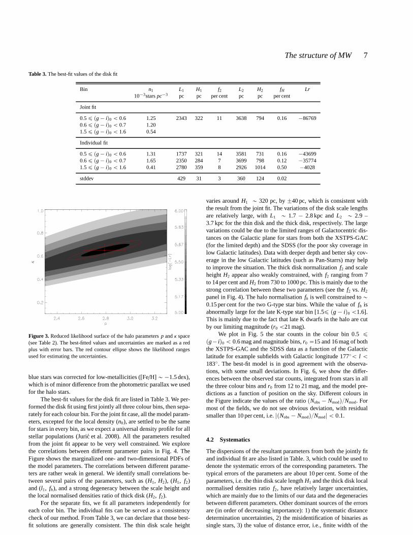
κ 0.1–1.0 0.01 0.65 0.05p 2.3–3.3 0.01 2.79 0.17

3 THE METHOD

3.1 The Galactic model

We adopt a three-components model for the smooth stellar distribu-tion of the Milky Way. It comprises two exponential disks (the thindisk and the thick disk) and a two-axial power-law ellipsoidhalo(Bahcall & Soneira 1980; Gilmore & Reid 1983). Thus the overallstellar densitynpR,Zq at a locationpR,Zq can be decomposed bythe sum of the thin disk, the thick disk and the halo,

npR,Zq “ D1pR,Zq ` D2pR,Zq ` HpR,Zq, (2)

whereR is the Galactocentric distance in the Galactic plane,Z isthe distance from the Galactic mid-plane.D1 and D2 are stellardensities of the thin disk and the thick disk,

DipR,Zq “ fi n0 exp

„

´pR´ Rdq

Li´

p|Z| ´ Zdq

Hi

, (3)

where the suffix i “ 1 and 2 stands for the thin disk and thick disk,respectively.Rd is the radial distance of the Sun to the Galacticcentre on the plane,Zd is the vertical distance of the Sun fromthe plane,n0 is the local stellar number density of the thin diskat (Rd, Zd), fi is the density ratio to the thin disk (f1=1), Li isthe scale-length andHi is the scale-height. We adoptRd “ 8 kpc(Reid & Majewski 1993) andZd “ 25 pc (Juric et al. 2008) in thecurrent work.H is the stellar density of the halo,

HpR,Zq “ fh n0

«

R2 ` pZ{κq2

R2d ` pZd{κq2

ff´p{2

, (4)

whereκ is the axis ratio,p is the power index andfh is the halonormalization relative to the thin disk.

3.2 Halo fit

We fit the component of the halo first. The metallicity distributionof the halo stars can be described as a single Gaussian component,with a median halo metallicity ofµH=´1.46 dex and spatially in-variant ofσH=0.30 dex (Ivezic et al. 2008). We assume the metal-licity of all halo stars as [Fe/H]“ ´1.46 dex and adopt the photo-metric parallax relation from Ivezic et al. (2008),

Mr “4.50´ 1.11rFe{Hs ´ 0.18rFe{Hs2

´ 5.06` 14.32pg ´ iq0 ´ 12.97pg ´ iq20

` 6.127pg ´ iq30 ´ 1.267pg ´ iq4

0 ` 0.0967pg ´ iq50.

(5)

The distances of the halo stars can thus be calculated from the stan-dard relation,

d “ 100.2pr0´Mr q`1. (6)

Star in a blue colour bin 0.5 ď g ´ i ă 0.6 are selected.They do not suffer from the giant star contamination and probelarger distances to constrain the halo. We calculate their distanceusing Equations (5) and (6). The distances of the disk stars will beunderestimated because they are more metal-rich. To exclude thecontamination of the disk stars, we use stars with absolute distance

to the Galactic plane|Z| ą 4 kpc. For each subfield, we divide allhalo stars into suitable numbers of logarithmic distance bins andthen count the number for each bin. This number can be modelledas,

NHpdq “ Hpdq∆Vpdq, (7)

whereHpdq is the halo stellar density given by Equation (4) and∆Vpdq is the volume, given by,

∆Vpdq “ω

3pπ

180q2pd3

2 ´ d31q, (8)

whereω denotes the area of the field (unit in deg2), d1 andd2 arethe lower distance limit and upper distance limit of the bin,respec-tively.

We fit the halo model parametersp andκ to the data. As weexplicitly exclude the disk, we cannot fit for the halo-to-thin disknormalization fh. A maximum likelihood technique is adopted toexplore the best values of those halo model parameters. In Table 2,we list the searching parameter space and the grid size. For each setof parameters, a reduced likelihood is computed between thesim-ulated data (star counts in bins of distances) and the observations,given by Bienayme et al. (1987) and Robin et al. (2014),

Lr “N

ÿ

i“1

qi ˆ p1 ´ Ri ` lnpRiqq, (9)

whereLr is the reduced likelihood for a binomial statistics,i is theindex of each distance bin,fi andqi are the number of stars in theith bin for the model and the data, respectively andRi “ fi{qi . Theuncertainties of the halo parameters are estimated similarly as thosein Chang et al. (2011). We calculate the likelihood for 1000 timesusing the observed data and the simulations of the best-fit modeladding with the Poisson noises. The resulted likelihood range de-fines the confidence level and thus the uncertainties.

3.3 Disk fit

The metallicity distribution of the disk is more complicated thanthat of the halo. Thus we fit the disk model parameters througha different way. We compare ther-band differential star counts indifferent colour bins and compare them to the simulations to searchfor the best disk model parameters (n0, L1, H1, f2, L2 andH2), aswell as the halo-to-thin disk normalizationfh.

Towards a subfield of galactic coordinates (l, b) and solid an-gleω, ther-band differential star countsNsimprk

0q (k is the index ofeach magnitude bin) in a given colour binpg´ iq j

0 ( j is the index ofeach colour bin) can be simulated as follows:

(i) The line of sight is divided into many small distance bins.For a given distance bin with centre distance ofdi (i is the index ofeach distance bin), ther-band apparent magnitude of a star is givenby

r0pdiq “ Mr ppg ´ iq j0, rFe{Hs|l, b,diq ` µ, (10)

whereµ is the distance modulus [µ “ 5log10pdiq ´ 5] and Mr isthe r-band absolute magnitude of the star given by Equation (5).The metallicities of halo stars are again assumed to be´1.46 dexand those of disk stars are given as a function of positions, whichis fitted using the metallicities of main sequence turn off stars fromLSS-GAC (Xiang et al. 2015),

rFe{Hs “ ´0.61` 0.51 ¨ expp´|Z|{1.57q. (11)

c© 2016 RAS, MNRAS000, 1–13

6 B.Q. Chen et al.

(ii) The number of stars in each distance bin can be calculatedby,

Npdiq “ npR,Z|l,b, diqVpdiq, (12)

whereVpdiq is the volume given by Equation (8) andnpR,Z|l,b,diqis the stellar number density given by Equation (2, 3 and 4). Thehalo model parameters,κ and p, resulted from the halo fit areadopted and settled to be not changeable here.

(iii) Combining all distance bins, we can obtain the modeledr-band star countsNprk

0q, by

Nprk0q “ ΣNpdiq whererk

0 ´rbin

2ă r0pdiq ă rk

0 `rbin

2, (13)

where rbin is the bin size ofr-band magnitude (we adoptrbin=1 mag in the current work).Nprk

0q is the underlying starcounts. When comparing to the observations, we need to applytheselection function, by

Nsimprk0q “ Nprk

0qSpl,b, g ´ i, rqC, (14)

whereSpl,b, g´ i, rq is the selection function, calculated by Equa-tion (1) for XSTPS-GAC subfields in GAC area and equals to onefor XSTPS-GAC subfields in M31/M33 area and all the SDSS sub-fields. Besides,

C “

#

1 for dmin ă di ă dmax;

0 otherwise;(15)

dmin “ 100.2prmin´Ar pdiq´Mr ppg´iq0,rFe{Hsqq`1, (16)

dmax “ 100.2prmax´Ar pdi q´Mr ppg´iq0,rFe{Hsqq`1, (17)

wherermin andrmax are the magnitude limits of each subfield. Weadopt rmin “ 12 andrmax “ 18 for all XSTPS-GAC subfields,and rmin “ 15 andrmax “ 21 for all SDSS subfields.Arpdiq isthe extinction inr-band at distance ofdi . We adopt the 3D ex-tinction map from Chen et al. (2014) for XSTPS-GAC subfields inGAC area and 2D extinction map from Schlegel et al. (1998) forXSTPS-GAC subfields in M31/M33 area and all SDSS subfields.As the size of each subfield is quite large („ 4 deg2), the extinctionArpdq varies within a subfield. We thus adopt the maximum valuesto make sure that our data are complete.

The photometric parallax relation of Equation (5) is only validfor the single stars. A large fraction of stars in the Milky Way areactually binaries (e.g. Yuan et al. 2015a). In the current work weadopt the binary fraction resulted from Yuan et al. (2015a) and as-sume that 40 per cent of the stars are binaries. The absolute mag-nitudesMr of the binaries are calculated as the same way as inYuan et al. (2015a).

We also consider the effects of photometric errors, the dis-persion of disk star metallicities and the errors due to the pho-tometric parallax relation of Ivezic et al. (2008). Ther-band pho-tometric errors of most stars in the XSTPS-GAC and the SDSSare smaller than 0.05 mag (Chen et al. 2014 for the XSTPS-GACand Sesar et al. 2006 for the SDSS). When we fit the metallici-ties of disk stars as a function of positions [Equation (11)], wefind a dispersion of the residuals of about 0.05 dex. According toEquation (5), this dispersion would introduce an offset of about0.05 mag for the absolute magnitude when [Fe/H] =´0.2 dex. As aresult, the effect of the photometric errors and the disk stars metal-licities dispersions would introduce a distance errors of smallerthan 5 per cent. Combining with the systematic error of the pho-tometric parallax relation, which is claimed to be smaller than10 per cent (Ivezic et al. 2008), we assume a total error of distance

of 15 per cent. This distance error is added when we model ther-band magnitude of stars in a given distance bin [Equation (10)].

We select three different colour bins for the disk fit. Two ofthem correspond to G-type stars with 0.5 ď pg ´ iq0 ă 0.6 magand 0.6 ď pg ´ iq0 ă 0.7 mag, and the other one corresponds tolate K-type stars with 1.5 ď pg ´ iq0 ă 1.6 mag. The giant andsub-giant contaminations for the first two G-type star bins are verysmall. For the late K-type stars, we exclude stars withr-band mag-nitude r0 ă 15 mag to avoid the giant contaminations. For eachcolour bin, we count the differentialr-band star counts with a bin-size of∆r “ 1 mag and then compare them to the simulations tosearch for the best disk model parameters, i.en0, L1, H1, f2, L2,

and H2 and the halo-to-thin disk normalizationfh. Similarly asin Robin et al. (2014), an ABC-MCMC algorithm is implementedusing the reduced likelihood calculated by Equation (9) in theMetropolis-Hastings algorithm acceptance ratio (Metropolis et al.1953; Hastings 1970). We note that the 68 per cent probability inter-vals of the marginalised probability distribution functions (PDFs)of each parameter, given by the accepted values after post-burn pe-riod in the MCMC chain are only the fitting uncertainties which donot include systematic uncertainties. A detailed analysisof errorsof the scale parameters will be given in Sect. 4.2.

The stellar flare is becoming significant atR ě15 kpc(Lopez-Corredoira & Molgo 2014) while the limiting magnitudewe adopt for XSTPS-GAC isr “ 18 mag, which corresponds toR „ 13 kpc for early G-type dwarfs. On the other hand, the diskwarp is a second order effect on the star counts and the XSTPS-GAC centre around the GAC, withl around 180˝. The effect of thedisk warp is thus negligible (Lopez-Corredoira et al. 2002). So inthe current work we ignore the influences of the disk warps andflares. In order to minimise the effects coming from other irregularstructures (overdensities) of the Galactic disk and halo (e.g., Virgooverdensity, etc. ), we iterate our fitting procedure to automaticallyand gradually remove pixels contaminated by unidentified irregu-lar structures, similarly as in Juric et al. (2008). The model is ini-tially fitted using all the data points. The resulted best-fitmodel isthen used to define the outlying data, which have ratios of resid-uals (data minus the best-fit model) to the best-fit model higherthan a given value, i.e.pNobs ´ Nmodq{Nmod ą a1. The model isthen refitted with the outliers excluded. The newly derived best-fitmodel is again compared to all the data points. New outliers withpNobs ´ Nmodq{Nmod ą a2 are excluded for the next fit. We repeatthis procedure with a sequence of valuesai = 0.5, 0.4, and 0.3. Theiteration, which gradually reject about 1, 5 and 15 per cent of theirregular data points of smaller and smaller significance, will makeour model-fitting algorithm to converge toward a robust solutionwhich describes the smooth background best.

4 THE RESULTS AND DISCUSSION

4.1 Fitting results

The best-fit halo model parameters obtained from the halo fit arelisted in Table 2 and the reduced likelihoodLr surface for the fit isshown in Fig. 3. TheLr contour dramatically changes alongκ, butrelatively mildly alongp. The best-fit halo model parameters areκ “ 0.65˘ 0.05 andp “ 2.79˘ 0.17. They are not surprisingly ingood agreement with those values from Juric et al. (2008), whichhaveκ “ 0.64 andp “ 2.8, since the data used for the halo fit inthe current work are mainly from the SDSS subfields. In addition,the photometric parallax relation that Juric et al. (2008)used for the

c© 2016 RAS, MNRAS000, 1–13

The structure of MW 7

Table 3.The best-fit values of the disk fit

Bin n1 L1 H1 f2 L2 H2 fH Lr10 3starspc 3 pc pc per cent pc pc per cent

Joint fit

0.5 ď pg ´ iq0 ă 0.6 1.25 2343 322 11 3638 794 0.16 ´867690.6 ď pg ´ iq0 ă 0.7 1.201.5 ď pg ´ iq0 ă 1.6 0.54

Individual fit

0.5 ď pg ´ iq0 ă 0.6 1.31 1737 321 14 3581 731 0.16 ´436990.6 ď pg ´ iq0 ă 0.7 1.65 2350 284 7 3699 798 0.12 ´357741.5 ď pg ´ iq0 ă 1.6 0.41 2780 359 8 2926 1014 0.50 ´4028

stddev 429 31 3 360 124 0.02

Figure 3. Reduced likelihood surface of the halo parametersp andκ space(see Table 2). The best-fitted values and uncertainties are marked as a redplus with error bars. The red contour ellipse shows the likelihood rangesused for estimating the uncertainties.

blue stars was corrected for low-metallicities ([Fe/H] „ ´1.5 dex),which is of minor difference from the photometric parallax we usedfor the halo stars.

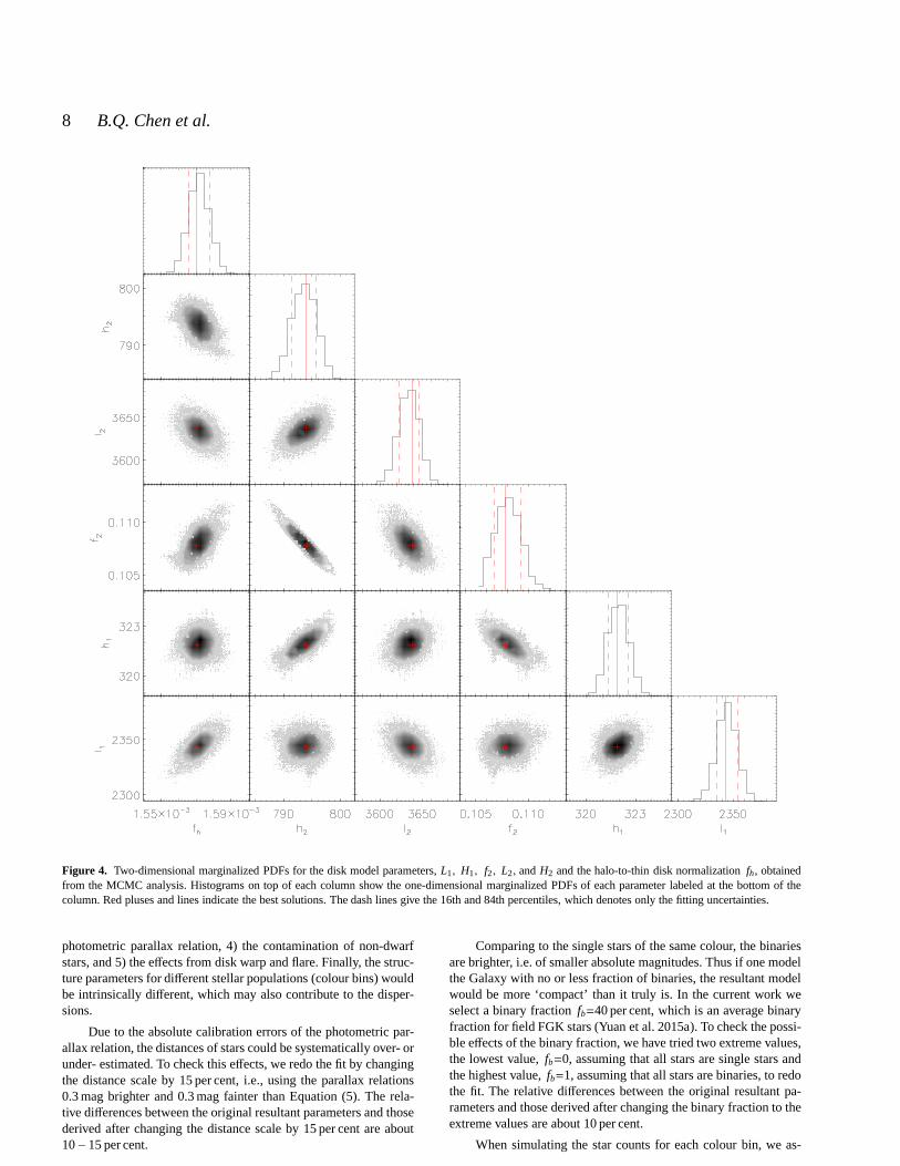
The best-fit values for the disk fit are listed in Table 3. We per-formed the disk fit using first jointly all three colour bins, then sepa-rately for each colour bin. For the joint fit case, all the model param-eters, excepted for the local density (n0), are settled to be the samefor stars in every bin, as we expect a universal density profile for allstellar populations (Juric et al. 2008). All the parameters resultedfrom the joint fit appear to be very well constrained. We explorethe correlations between different parameter pairs in Fig. 4. TheFigure shows the marginalized one- and two-dimensional PDFs ofthe model parameters. The correlations between different parame-ters are rather weak in general. We identify small correlations be-tween several pairs of the parameters, such as (H1, H2), (H1, f2)and (l1, fh), and a strong degeneracy between the scale height andthe local normalised densities ratio of thick disk (H2, f2).

For the separate fits, we fit all parameters independently foreach color bin. The individual fits can be served as a consistencycheck of our method. From Table 3, we can declare that those best-fit solutions are generally consistent. The thin disk scale height

varies aroundH1 „ 320 pc, by˘40 pc, which is consistent withthe result from the joint fit. The variations of the disk scalelengthsare relatively large, withL1 „ 1.7 ´ 2.8 kpc andL2 „ 2.9 –3.7 kpc for the thin disk and the thick disk, respectively. The largevariations could be due to the limited ranges of Galactocentric dis-tances on the Galactic plane for stars from both the XSTPS-GAC(for the limited depth) and the SDSS (for the poor sky coverage inlow Galactic latitudes). Data with deeper depth and better sky cov-erage in the low Galactic latitudes (such as Pan-Starrs) mayhelpto improve the situation. The thick disk normalizationf2 and scaleheightH2 appear also weakly constrained, withf2 ranging from 7to 14 per cent andH2 from 730 to 1000 pc. This is mainly due to thestrong correlation between these two parameters (see thef2 vs. H2

panel in Fig. 4). The halo normalisationfh is well constrained to„0.15 per cent for the two G-type star bins. While the value offh isabnormally large for the late K-type star bin [1.5ď pg ´ iq0 ă1.6].This is mainly due to the fact that late K dwarfs in the halo arecutby our limiting magnitude (r0 ă21 mag).

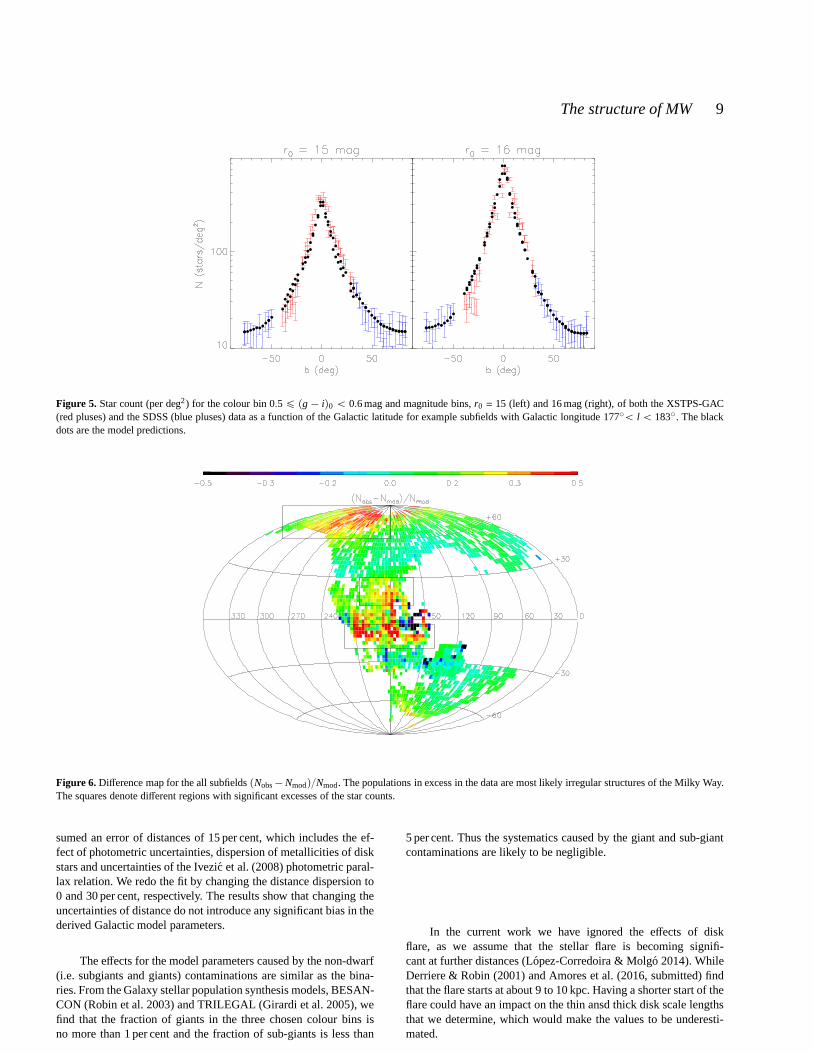
We plot in Fig. 5 the star counts in the colour bin 0.5 ďpg´ iq0 ă 0.6 mag and magnitude bins,r0 “15 and 16 mag of boththe XSTPS-GAC and the SDSS data as a function of the Galacticlatitude for example subfields with Galactic longitude 177˝ă l ă183˝. The best-fit model is in good agreement with the observa-tions, with some small deviations. In Fig. 6, we show the differ-ences between the observed star counts, integrated from stars in allthe three colour bins andr0 from 12 to 21 mag, and the model pre-dictions as a function of position on the sky. Different colours inthe Figure indicate the values of the ratiopNobs ´ Nmodq{Nmod. Formost of the fields, we do not see obvious deviation, with residualsmaller than 10 per cent, i.e.|pNobs ´ Nmodq{Nmod| ă 0.1.

4.2 Systematics

The dispersions of the resultant parameters from both the jointly fitand individual fit are also listed in Table. 3, which could be used todenote the systematic errors of the corresponding parameters. Thetypical errors of the parameters are about 10 per cent. Some of theparameters, i.e. the thin disk scale lengthH1 and the thick disk localnormalised densities ratiof2, have relatively larger uncertainties,which are mainly due to the limits of our data and the degeneraciesbetween different parameters. Other dominant sources of the errorsare (in order of decreasing importance): 1) the systematic distancedetermination uncertainties, 2) the misidentification of binaries assingle stars, 3) the value of distance error, i.e., finite width of the

c© 2016 RAS, MNRAS000, 1–13

8 B.Q. Chen et al.

Figure 4. Two-dimensional marginalized PDFs for the disk model parameters,L1, H1, f2, L2, andH2 and the halo-to-thin disk normalizationfh, obtainedfrom the MCMC analysis. Histograms on top of each column showthe one-dimensional marginalized PDFs of each parameter labeled at the bottom of thecolumn. Red pluses and lines indicate the best solutions. The dash lines give the 16th and 84th percentiles, which denotes only the fitting uncertainties.

photometric parallax relation, 4) the contamination of non-dwarfstars, and 5) the effects from disk warp and flare. Finally, the struc-ture parameters for different stellar populations (colour bins) wouldbe intrinsically different, which may also contribute to the disper-sions.

Due to the absolute calibration errors of the photometric par-allax relation, the distances of stars could be systematically over- orunder- estimated. To check this effects, we redo the fit by changingthe distance scale by 15 per cent, i.e., using the parallax relations0.3 mag brighter and 0.3 mag fainter than Equation (5). The rela-tive differences between the original resultant parameters and thosederived after changing the distance scale by 15 per cent are about10 – 15 per cent.

Comparing to the single stars of the same colour, the binariesare brighter, i.e. of smaller absolute magnitudes. Thus if one modelthe Galaxy with no or less fraction of binaries, the resultant modelwould be more ‘compact’ than it truly is. In the current work weselect a binary fractionfb=40 per cent, which is an average binaryfraction for field FGK stars (Yuan et al. 2015a). To check the possi-ble effects of the binary fraction, we have tried two extreme values,the lowest value,fb=0, assuming that all stars are single stars andthe highest value,fb=1, assuming that all stars are binaries, to redothe fit. The relative differences between the original resultant pa-rameters and those derived after changing the binary fraction to theextreme values are about 10 per cent.

When simulating the star counts for each colour bin, we as-

c© 2016 RAS, MNRAS000, 1–13

The structure of MW 9

Figure 5. Star count (per deg2) for the colour bin 0.5 ď pg ´ iq0 ă 0.6 mag and magnitude bins,r0 = 15 (left) and 16 mag (right), of both the XSTPS-GAC(red pluses) and the SDSS (blue pluses) data as a function of the Galactic latitude for example subfields with Galactic longitude 177ă l ă 183 . The blackdots are the model predictions.

Figure 6. Difference map for the all subfieldspNobs´ Nmodq{Nmod. The populations in excess in the data are most likely irregular structures of the Milky Way.The squares denote different regions with significant excesses of the star counts.

sumed an error of distances of 15 per cent, which includes theef-fect of photometric uncertainties, dispersion of metallicities of diskstars and uncertainties of the Ivezic et al. (2008) photometric paral-lax relation. We redo the fit by changing the distance dispersion to0 and 30 per cent, respectively. The results show that changing theuncertainties of distance do not introduce any significant bias in thederived Galactic model parameters.

The effects for the model parameters caused by the non-dwarf(i.e. subgiants and giants) contaminations are similar as the bina-ries. From the Galaxy stellar population synthesis models,BESAN-CON (Robin et al. 2003) and TRILEGAL (Girardi et al. 2005), wefind that the fraction of giants in the three chosen colour bins isno more than 1 per cent and the fraction of sub-giants is less than

5 per cent. Thus the systematics caused by the giant and sub-giantcontaminations are likely to be negligible.

In the current work we have ignored the effects of diskflare, as we assume that the stellar flare is becoming signifi-cant at further distances (Lopez-Corredoira & Molgo 2014). WhileDerriere & Robin (2001) and Amores et al. (2016, submitted) findthat the flare starts at about 9 to 10 kpc. Having a shorter start of theflare could have an impact on the thin ansd thick disk scale lengthsthat we determine, which would make the values to be underesti-mated.

c© 2016 RAS, MNRAS000, 1–13

10 B.Q. Chen et al.

4.3 Comparisons with other work

As stated in Section 4.1, our results of the halo model parametersare very similar as those derived from Juric et al. (2008), becauseof the similar method (stellar number density fits) and data (theSDSS) adopted in both work. The main differences in the halo fitbetween those from Juric et al. (2008) and our work are that theyadopt theχ2 fitting while we use the reduced likelihoodLr ; andthey calculate the number densities for the entire sample inpR, Zqspace while we do that separately for each line of sight. The resultin our work confirms those from Juric et al. (2008).

When constraining the disk model parameters, our methodand data are both quite different from those in Juric et al. (2008)but the results are in agreement at a level of about 10 per cent.However, Juric et al. (2008) admit that their result suffers largeuncertainties from the uncertainty in calibration of the photo-metric parallax relation and the poor sky coverages for the lowGalactic latitudes, which is not the case in our work. Gener-ally, our derived value of thin disk scale height, 322 pc, is inthe range of values, 150–360 pc, which resulted from the re-cent work by Bilir et al. (2008); Juric et al. (2008); Yaz & Karaali(2010); Chang et al. (2011); Polido et al. (2013); Jia et al. (2014)and Lopez-Corredoira & Molgo (2014). Specially, this value isin good agreement with the canonical value of 325 pc (Gilmore1984; Yoshii et al. 1987; Reid & Majewski 1993; Larsen 1996).Our derived value of the thin disk scale length, 2.3 kpc, is con-sistent with those results found by Ojha et al. (1996); Robinet al.(2000); Chen et al. (2001); Siegel et al. (2002); Karaali et al.(2007); Juric et al. (2008); Robin et al. (2012); Polido et al. (2013);Lopez-Corredoira & Molgo (2014) and Yaz Gokce et al. (2015),which ranges between 2 and 3 kpc. We find a local thick disk nor-malization of 11 per cent. In the different colour bins, this valuevaries between 7 and 14 per cent, probably because of the degener-acy with the scale height. It is well in agreement with the values inthe literature, which ranges between 7 and 13 per cent (Chen et al.2001; Siegel et al. 2002; Cabrera-Lavers et al. 2005; Juricet al.2008; Chang et al. 2011; Jia et al. 2014). The range of values forthe thick disk scale height and scale length from the recent lit-erature are respectively 600 – 1000 pc and 3 – 5 kpc (Bilir et al.2008; Juric et al. 2008; Yaz & Karaali 2010; Chang et al. 2011;Polido et al. 2013; Jia et al. 2014; Lopez-Corredoira & Molgo2014; Robin et al. 2014). The results deduced here, which havethick disk scale height of„800 pc and scale length of 3.6 kpc,are both in the middle of the ranges of those values reported inthe literature. Notice that there is a significant difference with theRobin et al. (2014) result for the thick disc. Their thick disk is mod-elled with 2 episodes, one of which has very similar parameters asthe present result (their old thick disk). But their young thick diskis more compact, with smaller scale height and scale length.Thedifference can be due to the different shapes used (they use secantsquared density laws and they include the flare) while in the presentstudy the thick disk is a simple exponential vertically.

5 SUBSTRUCTURES

One of the main purposes of the Galactic smooth structure mod-elling is to define the irregular structure of the Milky Way. Assum-ing that our model now reproduces the populations of the haloandthe disk, we can investigate if any further structures are missingfrom our modelling. As seen in Fig. 6, most of the significant devi-ations are overdensities, i.e.Nobs ą Nmod, except for a few subfields

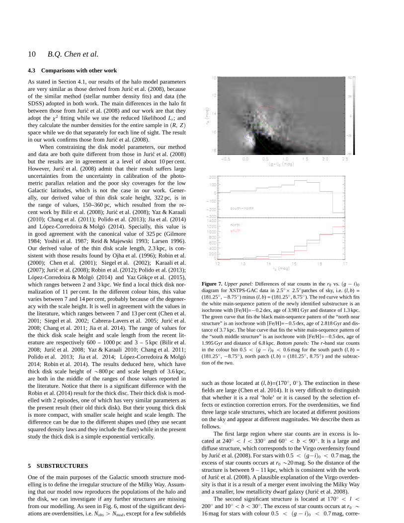
Figure 7. Upper panel:Differences of star counts in ther0 vs. pg ´ iq0

diagram for XSTPS-GAC data in 2.5˝ˆ 2.5 patches of sky, i.e. (l, b) =(181.25 , ´8.75 ) minus (l, b) = (181.25 , 8.75 ). The red curve which fitsthe white main-sequence pattern of the newly identified substructure is anisochrone with [Fe/H]=´0.2 dex, age of 3.981 Gyr and distance of 1.3 kpc.The green curve that fits the black main-sequence pattern of the “north nearstructure” is an isochrone with [Fe/H]=´0.5 dex, age of 2.818 Gyr and dis-tance of 3.7 kpc. The blue curve that fits the white main-sequence pattern ofthe “south middle structure” is an isochrone with [Fe/H]=´0.5 dex, age of1.995 Gyr and distance of 6.8 kpc.Bottom panels:The r-band star countsin the colour bin 0.5 ă pg ´ iq0 ă 0.6 mag for the south patch (l, b) =(181.25 , ´8.75 ), north patch (l, b) = (181.25 , 8.75 ) and the subtrac-tion of the two.

such as those located at (l,b)=(170˝, 0˝). The extinction in thesefields are large (Chen et al. 2014). It is very difficult to distinguishthat whether it is a real ‘hole’ or it is caused by the selection ef-fects or extinction correction errors. For the overdensities, we findthree large scale structures, which are located at different positionson the sky and appear at different magnitudes. We describe them asfollows.

The first large region where star counts are in excess is lo-cated at 240˝ ă l ă 330˝ and 60˝ ă b ă 90˝. It is a large anddiffuse structure, which corresponds to the Virgo overdensity foundby Juric et al. (2008). For stars with 0.5 ă pg´iq0 ă 0.7 mag, theexcess of star counts occurs atr0 „20 mag. So the distance of thestructure is between 9 – 11 kpc, which is consistent with the workof Juric et al. (2008). A plausible explanation of the Virgooverden-sity is that it is a result of a merger event involving the Milky Wayand a smaller, low metallicity dwarf galaxy (Juric et al. 2008).

The second significant structure is located at 170˝ ă l ă200˝ and 10˝ ă b ă 30˝. The excess of star counts occurs atr0 „16 mag for stars with colour 0.5 ă pg ´ iq0 ă 0.7 mag, corre-

c© 2016 RAS, MNRAS000, 1–13

The structure of MW 11

sponding to a distance between 1.5–2 kpc. This feature is consistentwith the so-called “north near structure” found by Xu et al. (2015).Juric et al. (2008) also report an overdensity atR= 9.5 kpc andZ= 0.8 kpc, which may be connected with this substructure. Xu etal.(2015) report that this substructure represents one of the locationsof peaks in the oscillations of the disk mid-plane, observedat about˘15˝Galactic latitude, toward the Galactic anticentre.

The third star counts excess structure is located at 150˝ ă l ă210˝ and´15˝ ă b ă ´5˝. We have not found any correspondingsubstructures to this feature from the literature. We need to checkfirst that whether this substructure is real or caused by the selectionbias or high extinction effects. To test its existence in a more directway, we examine the Hess diagrams constructed for a subfield lo-cated in the area of the feature and for a control subfield which isoutside the region. We choose the control subfield with the samegalactic longitude but opposite latitude as the selected subfield thatincludes the overdensity. To avoid the effect of the selection bias ofSample C, we select data from the complete XSTPS-GAC photo-metric sample in the regions (l,b) = (181.25˝, ´8.75˝, south field)and (181.25˝, 8.75˝, north field). Each region is of size 2.5˝ˆ 2.5˝.We correct the extinction of stars using the extinction map fromChen et al. (2015) together with the extinction law from Yuanet al.(2013). The average extinction for the south and north fieldsarerespectivelyAr = 0.66 and 0.27 mag. In Fig. 7, we show the dif-ferences between Hess diagrams and the star counts for starswithcolour 0.5ă pg´iq0 ă 0.6 mag for the two regions. We see a white-black-white main-sequence pattern in the difference Hess diagram.The fainter white sequence which indicating that there are morestars on the south side and the middle black sequence indicatingthat there are more stars on the north side respectively correspondto the “south middle structure” and “north near structure” describedin Xu et al. (2015). The bright white sequence corresponds tothenewly found substructure. Ther-band extinction in the these twofields are rather small. Even if we assume an error of 20 per centin extinction, the uncertainties of colourg ´ i and magnituder inthe two fields are onlyδg´i = 0.09 andδr = 0.13 for the south fieldandδg´i = 0.04 andδr = 0.05 for the north field, respectively. Theobserved feature will not be erased by adjusting the reddening val-ues. So we believe that the feature is real. The effect of selectionfunction and inaccuracies in the reddening correction cannot causethe apparent overdensities.

The excess of star counts occurs at aroundr0 „ 15 mag forstars in the colour ranges of 0.5ă pg ´ iq0 ă 0.6 mag, indicatinga distance between 1 – 1.5 kpc. We select a series of isochronesfrom An et al. (2009). The isochrone with [Fe/H] = ´0.2 dex andage of 3.981 Gyr, shifted by a distance of 1.3 kpc, fit well withthemaximum overdensities of the bright white sequence (see Fig. 7). The young age and high metallicity are consistent with those ofthe field thin disk stars. Thus we believe that this feature isun-likely a substructure originated from the outer disk. The distanceto the Galactic plane of this feature is aboutZ „ ´0.3 kpc andthat for the “north near structure” is aboutZ „ 0.5 kpc. Thesetwo features, which show the significant North-South asymmetryin the star number count distributions, are consistent withthe ver-tical oscillations in the stellar density in the solar neighbourhooddiscovered by Yanny & Gardner (2013, see their Fig. 18).

6 SUMMARY

Based on the data from the XSTPS-GAC and the SDSS, we havemodelled the global smooth structure of the Milky Way. We adopt a

three-component stellar distribution model. It comprisestwo dou-ble exponential disks, the thin disk and the thick disk, and atwo-axial power-law ellipsoid halo. The stellar number densityof halostars in the colour bin 0.5 ă pg´ iq0 ă 0.6 mag and ther-band dif-ferential star counts in three colour bins, 0.5 ă pg´ iq0 ă 0.6 mag,0.6 ă pg ´ iq0 ă 0.7 mag and 1.5 ă pg ´ iq0 ă 1.6 mag, are usedto determine the Galactic model parameters. The best-fit values arelisted in Table 2 and 3. In summary, the scale height and length ofthe thin disk areH1=322 pc andL1=2343 pc, and those of the thickdisk areH2=794 pc andL2=3638 pc. The local stellar density ratioof thick-to-thin disk isf2=11 per cent, and that of halo-to-thin diskis fh=0.16 per cent. The axis ratio and power-law index of the haloareκ “ 0.65 andp “ 2.79. Our results are all well constrained andin good agreement with the previous works.

By subtracting the observations from our best-fit model, wefind three large overdensities. Two of them have been previouslyidentified, including the Virgo overdensity in the Halo (Juric et al.2008), which located at 240˝ ă l ă 330˝ and 60˝ ă b ă 90˝ witha distance between 9 – 11 kpc, and the so-called “north near struc-ture” in the disk (Xu et al. 2015), which located at 170˝ ă l ă 200˝

and 10˝ ă b ă 30˝ with a distance between 1.5 – 2 kpc. The thirdstructure, located at 150˝ ă l ă 210˝ and´15˝ ă b ă ´5˝ witha distance between 1 – 1.5 kpc, is a new identification. Throughthe Hess diagram examination, we conclude that it could not bea artifact caused by extinction correction or selection effects. Thisfeature, together with the “north near structure” confirms the earlierdiscovery of Widrow et al. (2012) and Yanny & Gardner (2013) ofa significant Galactic North-South asymmetry in the stellarnumberdensity distribution.

ACKNOWLEDGEMENTS

We want to thank the referee, Prof. Gerry Gilmore, for his insight-ful comments. This work is partially supported by National KeyBasic Research Program of China 2014CB845700, China Post-doctoral Science Foundation 2016M590014 and National Natu-ral Science Foundation of China 11443006 and U1531244. TheLAMOST FELLOWSHIP is supported by Special Funding for Ad-vanced Users, budgeted and administrated by Center for Astronom-ical Mega-Science, Chinese Academy of Sciences (CAMS). Thisresearch has made use of the Chinese Virtual Observatory (China-VO) resources and services.

This work has made use of data products from the Guoshou-jing Telescope (the Large Sky Area Multi-Object Fibre Spectro-scopic Telescope, LAMOST). LAMOST is a National Major Sci-entific Project built by the Chinese Academy of Sciences. Fundingfor the project has been provided by the National Development andReform Commission. LAMOST is operated and managed by theNational Astronomical Observatories, Chinese Academy of Sci-ences.

Funding for SDSS-III has been provided by the Alfred P.Sloan Foundation, the Participating Institutions, the National Sci-ence Foundation, and the U.S. Department of Energy Office of Sci-ence. The SDSS-III web site is http://www.sdss3.org/. SDSS-III ismanaged by the Astrophysical Research Consortium for the Partici-pating Institutions of the SDSS-III Collaboration including the Uni-versity of Arizona, the Brazilian Participation Group, BrookhavenNational Laboratory, Carnegie Mellon University, University ofFlorida, the French Participation Group, the German ParticipationGroup, Harvard University, the Instituto de Astrofisica de Canarias,the Michigan State/Notre Dame/JINA Participation Group, Johns

c© 2016 RAS, MNRAS000, 1–13

12 B.Q. Chen et al.

Hopkins University, Lawrence Berkeley National Laboratory, MaxPlanck Institute for Astrophysics, Max Planck Institute for Ex-traterrestrial Physics, New Mexico State University, New York Uni-versity, Ohio State University, Pennsylvania State University, Uni-versity of Portsmouth, Princeton University, the Spanish Partici-pation Group, University of Tokyo, University of Utah, VanderbiltUniversity, University of Virginia, University of Washington, andYale University.

REFERENCES

Abazajian, K., et al. 2004, AJ, 128, 502Ak, S., Bilir, S., Karaali, S., & Buser, R. 2007, AstronomischeNachrichten, 328, 169

Alam, S., et al. 2015, ApJS, 219, 12Alves, D. R. 2000, ApJ, 539, 732An, D., et al. 2009, ApJ, 700, 523Bahcall, J. N. & Soneira, R. M. 1980, ApJ, 238, L17Bienayme, O., Robin, A. C., & Creze, M. 1987, A&A, 180, 94Bilir, S., Cabrera-Lavers, A., Karaali, S., Ak, S., Yaz, E.,& Lopez-Corredoira, M. 2008, PASA, 25, 69

Bilir, S., Karaali, S., Ak, S., Yaz, E., & Hamzaoglu, E. 2006a,New A., 12, 234

Bilir, S., Karaali, S., Guver, T., Karatas, Y., & Ak, S. G. 2006b,Astronomische Nachrichten, 327, 72

Bland-Hawthorn, J. & Gerhard, O. 2016, ArXiv e-printsBovy, J., Rix, H.-W., Liu, C., Hogg, D. W., Beers, T. C., & Lee,Y. S. 2012, The Astrophysical Journal, 753, 148

Cabrera-Lavers, A., Bilir, S., Ak, S., Yaz, E., & Lopez-Corredoira,M. 2007, A&A, 464, 565

Cabrera-Lavers, A., Garzon, F., & Hammersley, P. L. 2005, A&A,433, 173

Cabrera-Lavers, A., Gonzalez-Fernandez, C., Garzon, F., Ham-mersley, P. L., & Lopez-Corredoira, M. 2008, A&A, 491, 781

Chang, C.-K., Ko, C.-M., & Peng, T.-H. 2011, ApJ, 740, 34Chen, B., et al. 2001, ApJ, 553, 184Chen, B.-Q., Liu, X.-W., Yuan, H.-B., Huang, Y., & Xiang, M.-S.2015, MNRAS, 448, 2187

Chen, B.-Q., et al. 2014, MNRAS, 443, 1192Crane, J. D., Majewski, S. R., Rocha-Pinto, H. J., Frinchaboy,P. M., Skrutskie, M. F., & Law, D. R. 2003, ApJ, 594, L119

Creze, M. & Robin, A. 1983, in IAU Colloq. 76: Nearby Starsand the Stellar Luminosity Function, ed. A. G. D. Philip & A. R.Upgren, Vol. 76, 391

Derriere, S. & Robin, A. C. 2001, in Astronomical Society of thePacific Conference Series, Vol. 232, The New Era of Wide FieldAstronomy, ed. R. Clowes, A. Adamson, & G. Bromage, 229

Du, C., Ma, J., Wu, Z., & Zhou, X. 2006, MNRAS, 372, 1304Frinchaboy, P. M., Majewski, S. R., Crane, J. D., Reid, I. N.,Rocha-Pinto, H. J., Phelps, R. L., Patterson, R. J., & Munoz,R. R. 2004, ApJ, 602, L21

Gilmore, G. 1984, MNRAS, 207, 223Gilmore, G. & Reid, N. 1983, MNRAS, 202, 1025Girardi, L., Groenewegen, M. A. T., Hatziminaoglou, E., & daCosta, L. 2005, A&A, 436, 895

Hammersley, P. L., Garzon, F., Mahoney, T. J., Lopez-Corredoira,M., & Torres, M. A. P. 2000, MNRAS, 317, L45

Hastings, W. 1970, Monte Carlo sampling methods using Markovchains and their application.

Huang, Y., et al. 2015, Research in Astronomy and Astrophysics,15, 1240

Ibata, R. A., Irwin, M. J., Lewis, G. F., Ferguson, A. M. N., &Tanvir, N. 2003, MNRAS, 340, L21

Ivezic, Z., et al. 2008, ApJ, 684, 287Jia, Y., et al. 2014, MNRAS, 441, 503Juric, M., et al. 2008, ApJ, 673, 864Kaiser, N., et al. 2002, in Society of Photo-Optical Instrumenta-tion Engineers (SPIE) Conference Series, Vol. 4836, SurveyandOther Telescope Technologies and Discoveries, ed. J. A. Tyson& S. Wolff, 154–164

Karaali, S., Bilir, S., & Hamzaoglu, E. 2004, MNRAS, 355, 307Karaali, S., Bilir, S., Yaz, E., Hamzaoglu, E., & Buser, R. 2007,PASA, 24, 208

Larsen, J. A. 1996, PhD thesis, PhD Thesis, University of Min-nesota, (1996)

Liu, X.-W., et al. 2014, in IAU Symposium, Vol. 298, IAU Sym-posium, ed. S. Feltzing, G. Zhao, N. A. Walton, & P. Whitelock,310–321

Liu, X.-W., Zhao, G., & Hou, J.-L. 2015, Research in Astronomyand Astrophysics, 15, 1089

Lopez-Corredoira, M., Cabrera-Lavers, A., Garzon, F., &Ham-mersley, P. L. 2002, A&A, 394, 883

Lopez-Corredoira, M. & Molgo, J. 2014, A&A, 567, A106Majewski, S. R., Ostheimer, J. C., Rocha-Pinto, H. J., Patterson,R. J., Guhathakurta, P., & Reitzel, D. 2004, ApJ, 615, 738

Majewski, S. R., Skrutskie, M. F., Weinberg, M. D., & Ostheimer,J. C. 2003, ApJ, 599, 1082

Metropolis, N., Rosenbluth, A., Rosenbluth, M., Teller, A., &Teller, E. 1953, Equations of state calculations by fast computingmachines.

Momany, Y., Zaggia, S., Gilmore, G., Piotto, G., Carraro, G., Be-din, L. R., & de Angeli, F. 2006, A&A, 451, 515

Newberg, H. J., et al. 2002, ApJ, 569, 245Nishiyama, S., et al. 2005, ApJ, 621, L105Ojha, D. K., Bienayme, O., Robin, A. C., Creze, M., & Mohan,V.1996, A&A, 311, 456

Ortiz, R. & Lepine, J. R. D. 1993, A&A, 279, 90Perryman, M. A. C., et al. 2001, A&A, 369, 339Polido, P., Jablonski, F., & Lepine, J. R. D. 2013, ApJ, 778,32Reid, N. & Majewski, S. R. 1993, ApJ, 409, 635Reyle, C., Marshall, D. J., Robin, A. C., & Schultheis, M. 2009,A&A, 495, 819

Robin, A. C., Marshall, D. J., Schultheis, M., & Reyle, C. 2012,A&A, 538, A106

Robin, A. C., Reyle, C., & Creze, M. 2000, A&A, 359, 103Robin, A. C., Reyle, C., Derriere, S., & Picaud, S. 2003, A&A,409, 523

Robin, A. C., Reyle, C., Fliri, J., Czekaj, M., Robert, C. P., &Martins, A. M. M. 2014, A&A, 569, A13

Rocha-Pinto, H. J., Majewski, S. R., Skrutskie, M. F., & Crane,J. D. 2003, ApJ, 594, L115

Rocha-Pinto, H. J., Majewski, S. R., Skrutskie, M. F., Crane, J. D.,& Patterson, R. J. 2004, ApJ, 615, 732

Schlegel, D. J., Finkbeiner, D. P., & Davis, M. 1998, ApJ, 500,525

Sesar, B., et al. 2006, AJ, 131, 2801Siegel, M. H., Majewski, S. R., Reid, I. N., & Thompson, I. B.2002, ApJ, 578, 151

Skrutskie, M. F., et al. 2006, AJ, 131, 1163van Loon, J. T., et al. 2003, MNRAS, 338, 857Widrow, L. M., Gardner, S., Yanny, B., Dodelson, S., & Chen,H.-Y. 2012, ApJ, 750, L41

Wright, E. L., et al. 2010, AJ, 140, 1868

c© 2016 RAS, MNRAS000, 1–13

The structure of MW 13

Xiang, M.-S., et al. 2015, Research in Astronomy and Astro-physics, 15, 1209

Xu, Y., Newberg, H. J., Carlin, J. L., Liu, C., Deng, L., Li, J.,Schonrich, R., & Yanny, B. 2015, ApJ, 801, 105

Yanny, B. & Gardner, S. 2013, ApJ, 777, 91Yaz, E. & Karaali, S. 2010, New A., 15, 234Yaz Gokce, E., et al. 2015, PASA, 32, e012York, D. G., et al. 2000, AJ, 120, 1579Yoshii, Y., Ishida, K., & Stobie, R. S. 1987, AJ, 93, 323Yuan, H., Liu, X., Xiang, M., Huang, Y., Chen, B., Wu, Y., Hou,Y., & Zhang, Y. 2015a, ApJ, 799, 135

Yuan, H.-B., et al. 2015b, MNRAS, 448, 855Yuan, H. B., Liu, X. W., & Xiang, M. S. 2013, MNRAS, 430,2188

Zhang, H.-H., Liu, X.-W., Yuan, H.-B., Zhao, H.-B., Yao, J.-S.,Zhang, H.-W., & Xiang, M.-S. 2013, Research in Astronomy andAstrophysics, 13, 490

Zhang, H.-H., Liu, X.-W., Yuan, H.-B., Zhao, H.-B., Yao, J.-S.,Zhang, H.-W. Xiang, M.-S., & Huang, Y. 2014, Research in As-tronomy and Astrophysics, 14, 456

c© 2016 RAS, MNRAS000, 1–13