Construction of Geometric Outer-Measures and …loring/graduate_students/DaveWorth...Construction of Geometric Outer-Measures and Dimension Theory by David Worth B.S., Mathematics,

Construction of GeometricOuter-Measures and Dimension Theory

by

David Worth

B.S., Mathematics, University of New Mexico, 2003

THESIS

Submitted in Partial Fulfillment of the

Requirements for the Degree of

Master of Science

Mathematics

The University of New Mexico

Albuquerque, New Mexico

December, 2006

c©2008, David Worth

iii

DEDICATION

To my lovely wife Meghan, to whom I am eternally grateful for her support and

love. Without her I would never have followed my education or my bliss.

iv

ACKNOWLEDGMENTS

I would like to thank my advisor, Dr. Terry Loring, for his years of encouragementand aid in pursuing mathematics. I would also like to thank Dr. Cristina Pereyra forher unfailing encouragement and her aid in completing this daunting task. I wouldlike to thank Dr. Wojciech Kucharz for his guidance and encouragement for theentirety of my adult mathematical career.

Moreover I would like to thank Dr. Jens Lorenz, Dr. Vladimir I Koltchinskii, Dr.James Ellison, and Dr. Alexandru Buium for their years of inspirational teachingand their influence in my life.

v


by

David Worth

ABSTRACT OF THESIS

Submitted in Partial Fulfillment of the

Requirements for the Degree of

Master of Science

Mathematics

The University of New Mexico

Albuquerque, New Mexico

December, 2006


by

David Worth

B.S., Mathematics, University of New Mexico, 2003

M.S., Mathematics, University of New Mexico, 2008

Abstract

Geometric Measure Theory is the rigorous mathematical study of the field commonly

known as Fractal Geometry. In this work we survey means of constructing families of

measures, via the so-called “Caratheodory construction”, which isolate certain small-

scale features of complicated sets in a metric space. The construction is explicit and

covered in great detail, after which specific instances of constructed measures are

investigated in depth. The work then investigates another related by fundamentally

different class of measures, the “packing measures”, and the two classes are compared.

Finally, certain important dimensional ideas are investigated in detail including some

oddities of the field.

vii

Contents

List of Figures . . . . . . . . . . . . . . . . . . . . . . . . . . . . . . . . . . x

List of Examples . . . . . . . . . . . . . . . . . . . . . . . . . . . . . . . . xi

1 Introduction 1

1.1 Background . . . . . . . . . . . . . . . . . . . . . . . . . . . . . . . . 1

1.2 Overview . . . . . . . . . . . . . . . . . . . . . . . . . . . . . . . . . . 2

2 Mathematical Foundations 4

2.1 Set Theory and Analytic Background . . . . . . . . . . . . . . . . . . 4

2.2 Topological Background . . . . . . . . . . . . . . . . . . . . . . . . . 6

2.3 Measure Theoretic Background . . . . . . . . . . . . . . . . . . . . . 9

3 Caratheodory Geometric Measures 15

3.1 Caratheodory Construction . . . . . . . . . . . . . . . . . . . . . . . 16

3.2 Hausdorff Measures . . . . . . . . . . . . . . . . . . . . . . . . . . . . 23

3.2.1 Calculating Hausdorff Measures . . . . . . . . . . . . . . . . . 29

viii

Contents

3.2.2 Geometric Interpretation of Integral Dimension Hausdorff Mea-

sures . . . . . . . . . . . . . . . . . . . . . . . . . . . . . . . . 34

3.2.3 Generalized Hausdorff Measures . . . . . . . . . . . . . . . . . 42

3.3 Spherical Outer-Measures . . . . . . . . . . . . . . . . . . . . . . . . 42

3.4 Net Outer-Measures . . . . . . . . . . . . . . . . . . . . . . . . . . . 44

4 Packing Outer-Measures 47

4.1 A “Dual” Construction? . . . . . . . . . . . . . . . . . . . . . . . . . 58

5 Dimension Theory 60

5.1 Hausdorff Dimension . . . . . . . . . . . . . . . . . . . . . . . . . . . 60

5.2 Packing Dimension . . . . . . . . . . . . . . . . . . . . . . . . . . . . 69

5.3 Comparison of Dimensions . . . . . . . . . . . . . . . . . . . . . . . . 71

6 Conclusion 73

List of Notation 75

References 76

ix

List of Figures

Description Page

Approximations to the Koch Curve 36

Approximations to the Peano Curve 37

x

List of Examples

Description Page

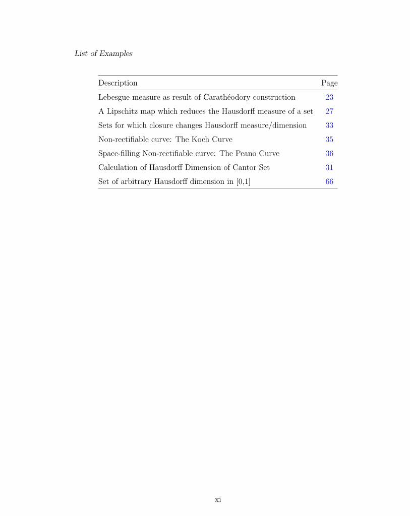
Lebesgue measure as result of Caratheodory construction 23

A Lipschitz map which reduces the Hausdorff measure of a set 27

Sets for which closure changes Hausdorff measure/dimension 33

Non-rectifiable curve: The Koch Curve 35

Space-filling Non-rectifiable curve: The Peano Curve 36

Calculation of Hausdorff Dimension of Cantor Set 31

Set of arbitrary Hausdorff dimension in [0,1] 66

xi

Chapter 1

Introduction

1.1 Background

The study of Geometric Measure Theory, often referred to as “Fractal Geometry”,

has roots in physics, mathematics, and in fields as concrete as geography. The

grey area between mathematics and physics is realized in the study of stochastic

systems; in geography the study of coastlines led to “fractal structures” as observed

by Richardson [BM83, pg. 33]; and in pure mathematics functions of complicated fine

structure were realized by Karl Weierstrass (1872) in functions without derivatives

anywhere [GAE04, pg. 3], Helge Von Koch (1904) in non-rectifiable curves [GAE04,

pg. 25], and later, and in great depth, by A.S. Besicovitch and Felix Hausdorff1.

1To avoid merely copying the table of contents of Gerald Edgar’s encyclopedic workdocumenting the mathematical foundations of modern Fractal Geometry/Geometric Mea-sure Theory the author recommends that the reader new to the area find a copy of Edgar’sClassics on Fractals, in which he has collected, cataloged, and annotated the major earlypapers in the field, and included recommendations for further reading. [GAE04]

1

Chapter 1. Introduction

1.2 Overview

Geometric measure theory is the name for the modern mathematical framework

in which to discuss “fractal geometry” as it is understood by mathematicians and

physicists.

The primary goal of this work is to discuss the constructive methods used for

generating so-called “Geometric Measures” with some abstract machinery, and to

prove in great generality, properties of the constructed measures. There are actually

two general families of incompatible measures discussed. The incompatibility is

discussed as a side effect of their varying constructions, and comparisons between

the two families, as specialized as they are, are discussed.

We begin with a minimal amount of analysis, including topology and measure

theory, enough to provide the necessary definitions for the rest of the work but little

enough that the subject cannot be learned only from the provided foundations. A

basic undergraduate or early graduate background in those subjects is expected and

required for the remainder of the text.

The next focus is the Caratheodory construction and the so-called “Caratheodory

geometric measures”, which are the measures derived from the construction. The

most famous of these measures, the family of Hausdorff measures (or Hausdorff-

Besicovitch measures) is pursued in some depth, including some explicit calculations

and constructions of sets with a given measure. We also discuss two other classes of

measures, closedly related to the Hausdorff measure, the spherical and net measures,

which provide bounds on the family of Hausdorff outer-measures in terms of more

easily visualized and worked with covering sets.

A more active subject is then explored, that of the packing measures, introduced

by Taylor and Tricot [SJTCT85]. The family of packing measures is in many respects

2

Chapter 1. Introduction

a family of measures “dual” to the Hausdorff measures but fundamentally different

in the sets which they measure effectively.

The final subject of importance in the text is that of dimension theory and two

dimensions of sets derived from the Hausdorff and packing outer-measure families.

These dimensions are related to the topological dimension in important ways; so

much so that Mandelbrot defined a “fractal” in terms of the relationship between

the topological dimension and the Hausdorff dimensions [BM83, pg. 15].

3

Chapter 2

Mathematical Foundations

2.1 Set Theory and Analytic Background

Notation. By countable we mean either a finite set or a countable set in the usual

sense of a set which can be put in 1-1 correspondence with the natural numbers,

denoted by N

Notation. Let X be a set, then by P(X) we denote the power-set of X.

Definition 2.1.1. Let (X, d) be a metric space. A function f : X → X is called

Lipschitz with constant c if d(f(x), f(y)) ≤ cd(x, y) for all x, y ∈ X.

Of course there is a more general notion of Lipschitz with f mapping between two

different metric spaces but the modification of the definition is obvious. Moreover if

the explicit Lipschitz constant is not listed then one assumes it exists as needed.

Definition 2.1.2. Let V be a linear subspace of the normed vector space (Rn, || · ||),

and let A ⊆ Rn. We denote the orthogonal projection of A onto V by PrV (A) =

{PrV (a) : a ∈ A}.

4

Chapter 2. Mathematical Foundations

Lemma 2.1.3. Let V be a linear subspace of the complete normed vector space

(Rn, || · ||). PrV is Lipschitz of constant 1.

Proof. By the projection theorem (see Royden [HLR68, pg. 214, #53]) we may write

x = v + w where v ∈ V and w ∈ V ⊥. Then

||PrV (x)|| = ||PrV (v + w)|| = ||PrV (v) + PrV (w)|| = ||v|| ≤ ||v + w|| = ||x||

Using this result we see that by replacing x with x− y we have

||PrV (x)− PrV (y)|| = ||PrV (x− y)|| ≤ ||x− y||

so PrV is Lipschitz with constant 1.

Definition 2.1.4. A function φ : [0,∞) → [0,∞) is called Hausdorff if it is non-

decreasing, continuous, φ(0) = 0 and φ(t) > 0 for all t > 0.

It should be noted that various authors require that a Hausdorff function be

continuous from the right at zero but as a matter of convenience we choose continuity

everywhere. This approach is consistent with the work of McClure [MM94, pg. 5]

and Hasse [HH86] (who only insists that the function be zero at zero and continuous)

and presents no clear limitation to the theory. To the contrary, several useful results

become untrue if we drop the continuity assumption.

Lemma 2.1.5. The composition of two Hausdorff functions is Hausdorff.

Proof. Let h, g be Hausdorff, and let f = h ◦ g. f(0) = h(g(0)) = h(0) = 0 and let

t > 0 then if t0 = g(t) then t0 > 0. f(t) = h(g(t)) = h(t0) > 0 since h is Hausdorff

so f is Hausdorff.

Example 2.1.6. Let fs : [0,∞) → [0,∞), fs(t) = ts, then fs is Hausdorff for all

s > 0.

5


2.2 Topological Background

Notation. Throughout this section let (X, || · ||) be a normed vector space over some

field F , and let A ⊆ X, x ∈ X, and c ∈ F , and let Y by a topological space, unless

otherwise noted.

For this paper we will only concern ourselves with real vector spaces unless oth-

erwise noted. We state those results which we can in great generality, but when

specificity is required the real case is used.

Notation. Let x ∈ X and let r > 0. We denote by B(x, r) = {a ∈ X : d(x, a) < r},

the open ball of radius r about the point x. We denote by B(x, r) = {a ∈ X :

d(x, a) ≤ r}, the closed ball of radius r about the point x.

Definition 2.2.1. By the diameter of a set A in a normed vector space we mean

diam(A) = sup{||x − y|| : x, y ∈ A}. For brevity we use the notation d(A) =

diam(A). If we are in an arbitrary metric space (X, d) we write d(A) = sup{d(x, y) :

x, y ∈ A} for the diameter.

Definition 2.2.2. By a translation of A by x, denoted A + x, we mean the set

{a+ x : a ∈ A}.

Lemma 2.2.3. diam(·) is translationally invariant.

Proof. By definition for any U ⊆ X and any x ∈ X, U + x = {u + x : u ∈ U}. So

for u1, u2 ∈ U + x there are u′1, u′2 ∈ U such that u1 = u′1 + x and u2 = u′2 + x.

So

d(U + x)def= sup{||u1 − u2|| : u1, u2 ∈ U + x}

= sup{||(u′1 + x)− (u′2 + x)|| : u′1, u′2 ∈ U}

= sup{||u′1 − u′2|| : u′1, u′2 ∈ U}def= d(U)

6


Definition 2.2.4. Let A ⊆ X and c ∈ F . By a scaling of A by c, denoted by cA,

we mean the set {ca : a ∈ A}.

Lemma 2.2.5. Let (X, || · ||) be a normed vector space over R. If c ∈ (0,∞) then

d(cA) = cd(A).

Proof.

d(cA)def= sup{||x− y|| : x, y ∈ cA}

= sup{||cx0 − cy0|| : x0, y0 ∈ A}

= sup{c||x0 − y0|| : x0, y0 ∈ A}

= cd(A)

Definition 2.2.6. Fix δ ∈ (0,∞). A δ-cover of A is countable collection of subsets

of X, {Ui}∞i=1, such that A ⊆⋃i Ui and d(Ui) ≤ δ.

Lemma 2.2.7. Let {Ui} be a δ-cover of A, then {Ui + x} is a δ-cover of A+ x.

Proof. Let y ∈ A, then y ∈ Ui for some i. Then y+x ∈ Ui+x and y+x ∈ A+x, both

by the definition of translation. Since this holds for every y ∈ A and d(Ui) = d(Ui+x)

by Lemma 2.2.3, {Ui + x} is a δ-cover of A+ x.

Lemma 2.2.8. Let {Ui} be a δ-cover of A, then {cUi} is a (cδ)-cover of cA for all

c ∈ (0,∞).

Proof. Let y ∈ A then y ∈ Ui for some i. Then cy ∈ cUi and cy ∈ cA, but this is

true for all y ∈ A so {cUi} is a cover of A, and by Lemma 2.2.5 {cUi} is a (cδ)-cover

of cA.

7


Definition 2.2.9. Two setsA,B ⊂ X are positively separated if d(A,B) = inf{d(a, b) :

a ∈ A, b ∈ B} > 0.

The following theorem is a nice topological result, the proof of which is straight-

forward (and may be found in Edgar [GAE91, pg. 58]) but the result useful later.

Theorem 2.2.10. Let (X, d) be a metric space, A ⊆ X be closed, and B ⊆ X be

compact. If A ∩B = ∅ then dist(A,B) > 0.

Proof. Assume dist(A,B) = 0 then there exist 〈xn〉 ⊂ A, 〈yn〉 ⊂ B such that

d(xn, yn) < 1/n. Since B is compact we may pass to a convergent sub-sequence (also

called 〈yn〉) with the property that yn → y ∈ B as n→∞. Then xn → y as n→∞

by assumption but since A is closed y ∈ A thus A ∩B 6= ∅, a contradiction.

So dist(A,B) > 0.

Example 2.2.11. It should be noted that the compactness of the second set is

necessary in the hypotheses since the following two sets are both closed and disjoint

but the distance between them is zero. Let A = R×{0} (essentially the x-axis in the

plane) and B = {(x, 1/x) : x ∈ R} (essentially the graph of the function f(x) = 1/x).

Both are closed since their complements are open, but neither are compact since

neither is bounded (by the Heine-Borel Theorem). Moreover dist(A,B) = 0.

Corollary 2.2.12. Disjoint compact sets in Rn are positively separated.

Proof. By Heine-Borel compact sets are closed and bounded in Rn thus we simply

apply the above theorem directly.

Definition 2.2.13. A topological space Y is called Hausdorff if given two points

x, y ∈ Y with x 6= y then there exist open sets U, V ⊂ Y such that x ∈ U, y ∈ V and

U ∩ V = ∅.

8


Definition 2.2.14. A Hausdorff topological space Y is called locally compact if for

every x ∈ Y there exists an open set U ⊂ Y such that the closure of U , denoted U ,

is compact.

Example 2.2.15. (Rn, || · ||2), with || · ||2 being the Euclidean norm, is a locally

compact normed vector space over R.

Note. For the majority of this work if we discuss the topology of Rn we assume it is

equipped with the Euclidean norm (and subsequently the Euclidean metric).

Lemma 2.2.16. Let (X, d) be a metric space, and let A ⊂ X be a bounded set, then

for all a ∈ A, A ⊆ B(a, d(A)).

Proof. Fix a0 ∈ A, then for any a ∈ A d(a0, a) < d(A) by definition of diameter,

thus A ⊆ B(a0, d(A)). Since the result is independent of our choice of a0 the lemma

follows.

2.3 Measure Theoretic Background

Definition 2.3.1. Given a set X, a function ν : P(X)→ [0,∞] is an outer-measure

if

1. ν(∅) = 0

2. For A ⊆ A′ ⊆ X, ν(A) ≤ ν(A′)

3. For {Ai}∞i=1 ⊂P(X), ν (⋃∞i=1Ai) ≤

∑∞i=1 ν(Ai)

Note. Halmos’ definition of an outer-measure is identical [PH64, pg. 42], but stated

as “An outer measure is an extended real valued, non negative, monotone, and count-

ably subadditive set function ...” It is important to note that countable subadditivity

is defined as above for outer measures rather than additivity as one has for measures.

9


Definition 2.3.2. Given an outer-measure ν, a set B is ν-measurable in the sense

of Caratheodory if and only if for all A ⊆ X arbitrary we have ν(A) = ν(A ∩ B) +

ν(A \B).

Note. For the duration of this work when we refer to a set as measurable we mean

measurable in the sense of Caratheodory.

Notation. We denote the set of all ν-measurable subsets of X (in the sense of

Caratheodory) by M (X, ν).

The credit given to Caratheodory in this specific definition of measurability comes

from Gerald Edgar [GAE91, pg. 130]. This definition may also be found in Hal-

mos [PH64, pg. 44] and Royden [HLR68, pg. 251], but Caratheodory is not named.

Royden provides an alternate definition of measurability [HLR68, pg. 296] using

the notion of measurable functions. For further information please see Royden’s

exposition on the subject.

In the geometric measure theory literature very often an outer-measure is simply

referred to as a measure. We hold the convention that a measure is an outer-measure

where the sub-additivity condition is stronger in that if {Ai}∞i=1 ⊂M (X, ν) ⊂P(X)

are such that Ai ∪ Aj = ∅ for i 6= j then we have ν (⋃∞i=1Ai) =

∑∞i=1 ν(Ai). Alter-

natively we may take a measure to be an outer-measure restricted to a σ-algebra of

measurable sets where this subadditivity condition holds as the following Theorem

of Caratheodory’s (as found in Bauer [HB01, pg. 21] and paraphrased here with

consistent notation) states:

Theorem 2.3.3. Let ν be an outer-measure on a set X, then the system A of ν-

measurable subsets of X is a σ-algebra. Moreover the restriction of ν to A is a

measure.

Definition 2.3.4. Let X be a locally compact Hausdorff topological space. An

outer-measure ν on X is a metric outer-measure if given two positively separated

10


sets A,A′ ⊆ X then ν(A ∪ A′) = ν(A) + ν(A′).

Remark. Since normed vector spaces are metric spaces, and thus locally compact

Hausdorff, the definition of metric outer-measure (Def. 2.3.4) applies immediately to

any normed vector space

Example 2.3.5. The n-dimensional Lebesgue Outer-Measure, Ln is a metric outer-

measure. This outer-measure may be constructed explicitly, and all of its properties

proven independently or it may be constructed using abstract machinery, as we do

in Example 3.1.16.

The following technical lemma on the continuity of metric outer-measures is nec-

essary:

Lemma 2.3.6 (Caratheodory’s Lemma). Let ν be a metric outer-measure in some

metric space (X,d), 〈An〉 an increasing sequence of subsets of X such that A =

limn→∞

An and d(Aj, A \ Aj+1) > 0 for all j then limn→∞

ν(An) = ν(A).

Proof. By the definition of outer-measure we have ν(Aj) ≤ ν(A) for all j thus

limj→∞

ν(Aj) ≤ ν(A) so we need ν(A) ≤ limj→∞

ν(Aj).

We begin by setting B1 = A1 and Bj = Aj+1 \ Aj so we have A =∞⋃j=1

Bj and

because ν is metric and d(B2i, B2j) > 0 by hypothesis (similarly for the odd indices)

we have the following equalities:

ν(∞⋃i=1

B2i) =∞∑i=1

ν(B2i) and ν(∞⋃i=1

B2i−1) =∞∑i=1

ν(B2i−1)

We assume both series converge otherwise ν(A) =∞. So the following inequali-

ties hold:

11


ν(A) = ν(∞⋃i=1

Ai)

= ν

(Aj ∪

(∞⋃

i=j+1

Bi

))

≤ ν(Aj) + ν(∞⋃

i=j+1

Bi)

≤ ν(Aj) +∞∑

i=j+1

ν(Bi)

and since the series converges the tail goes to zero as j →∞.

The first inequality is by the fact that ν is metric and the second is by mono-

tonicity of ν. So we have ν(A) ≤ limj→∞

ν(Aj) thus ν(A) = limj→∞

ν(Aj).

Definition 2.3.7. The Borel Sets in Rn are the smallest σ-algebra generated by the

open (resp. closed, compact) sets of Rn.

For a definition and formal exposition regarding the Borel sets, see Halmos [PH64,

pg. 153] or Bauer [HB01, pg. 27].

Definition 2.3.8. An outer-measure (or measure) ν is Borel if the Borel sets are

measurable.

Theorem 2.3.9 (Caratheodory’s Criterion). An outer-measure ν on a metric space

(X, d) is Borel if and only if ν is metric.

Proof. The following proof that if ν is metric then ν is Borel is from Falconer [KJF85,

Thm. 1.5, pg. 6] and relies heavily on Caratheodory’s Lemma [2.3.6].

Let ν be a metric outer-measure on (X, d). Since the Borel σ-algebra is the

smallest σ-algebra generated by the closed sets we may consider E ⊂ X closed and

A ⊂ X arbitrary.

12


Define the sets Aj = {a ∈ A\E : d(a,E) ≥ 1j}. {Aj} is increasing, i.e. Aj ( Aj+1.

Since E is closed we have limj→∞

Aj =∞⋃j=1

Aj = A \ E. Moreover d(A ∩ E,Aj) ≥ 1j

so

we have, since ν is metric, ν(A ∩ E) + ν(Aj) = ν((A ∩ E) ∪ Aj) ≤ ν(A) where the

final inequality is by the monotonicity of ν since (A∩E), Aj ( A are disjoint for all

j.

To apply Caratheodory’s Lemma we need d(Aj, (A \E) \Aj+1) > 0 for all j. Let

x ∈ (A \E) \Aj+1, then there exists z ∈ E such that d(x, z) < 1j+1

by definition. So

if y ∈ Aj then

d(x, y) + d(y, z) ≤ d(x, z) <1

j + 1

By subtracting and multiplying by −1 we have

d(x, y) ≥ d(y, z) + d(x, z) ≥ 1

j− 1

j + 1> 0

So via Caratheodory’s Lemma we have limj→∞

ν(Aj) = ν(A \E). As above we have

ν(A ∩ E) + ν(A \ E) = ν(A ∩ E) + limj→∞

ν(Aj)

= limj→∞

ν((A ∩ E) ∪ Aj)

= ν((A ∩ E) ∪ A \ E)

= ν(A)

So ν is Borel.

Conversely, let ν be Borel and let A,A′ ⊂ X such that d(A,A′) = δ > 0. Define

Aε = {x ∈ X : d(x,A) < ε = δ/3}

then A ⊆ Aε and d(Aε, A′) > 0 which implies Aε ∩ A′ = ∅. By construction Aε

is open and thus Borel so since ν is Borel and by the Caratheodory definition of

measurability we get the following:

ν(A ∪ A′) = ν((A ∪ A′) ∩ Aε) + ν((A ∪ A′) \ Aε) = ν(A) + ν(A′)

13


So ν is metric.

Note that to prove that ν Borel implies ν metric one may replace Aε with A and

the same proof goes through.

Definition 2.3.10. An outer-measure ν is outer-regular if given a set A there exists

a ν-measurable set U such that A ⊆ U and ν(A) = ν(U).

Definition 2.3.11. An outer-measure ν is Borel-regular if given a set A there exists

a Borel set B such that A ⊆ B and ν(A) = ν(B).

Note that Borel regular implies outer-regular for any Borel outer-measure (or

measure) ν; in other words, Borel regularity is a stronger condition than outer-

regularity.

Definition 2.3.12. An outer-measure (or measure) ν is Radon if the following con-

ditions are met:

• ν is Borel

• ν(K) <∞ for all K ⊂ X compact.

• ν(U) = sup {ν(K) : K compact , K ⊂ U} for all open U ⊆ X.

• ν(A) = inf {ν(U) : A ⊆ U ⊆ X,U open } for A ⊆ X.

Definition 2.3.13. Let (X, || · ||) be a normed vector space. An outer-measure ν on

X is translationally invariant if ν(A) = ν(A+ x) for all A ⊆ X and x ∈ X.

Example 2.3.14. The n-dimensional Lebesgue outer-measure Ln on Rn is transla-

tionally invariant and a Radon measure. This is clear since by Heine-Borel compact

sets are closed and bounded, and bounded measurable sets have finite measure with

respect to Ln. The fact that Ln is Borel is well understood (see Halmos [PH64, pg.

153]).

14

Chapter 3

Caratheodory Geometric Measures

This section is entitled “Caratheodory Geometric Measures,” but a great deal of the

chapter discusses specific details of the Hausdorff measure, a specific instance of a

“Caratheodory measure”, or more accurately, a family thereof. We first introduce

the “Caratheodory construction”, an abstract piece of machinery for constructing

metric outer-measures on a given metric space. Often that metric space is Rn but

this constraint is not necessary for the general construction which may take place in

a more general metric space within the stated constraints.

The best understood, or at least most general, of the outer-measures constructed

by the Caratheodory construction is the family of Hausdorff outer-measures. This

family is often referred to as the Hausdorff-Besicovitch outer-measures by influ-

ential members of the mathematical community, including Benoit Mandelbrot in

The Fractal Geometry of Nature [BM83, pg. 15]. This family of outer-measures has

a straight-forward construction in terms of the Caratheodory method, but gener-

ating useful lower bounds on the outer-measures of certain sets is difficult, so we

introduce two other families of outer-measures which provide approachable bounds

for the Hausdorff outer-measures in terms of more tractable sets. These two families

15

Chapter 3. Caratheodory Geometric Measures

of measures, the so-called spherical and net measures, are generated out of simple

sets and are bounded by the Hausdorff outer-measures with “nice” coefficients.

The use of the term “Caratheodory Geometric Measures” appears unique to this

work after a survey of related works. This naming scheme was chosen for two rea-

sons: First, it groups a large class of metric outer-measures under an umbrella term

allowing them to be considered together as a family, and secondly it distinguishes

them from another important class of outer-measures, the packing measures, and

allows one to discuss the difference between the two classes easily.

Throughout this section, unless otherwise noted, let (X, ||·||) be a locally compact

normed vector space. In all cases for simplicity X may be simply thought of as Rn

with the standard Euclidean topology.

3.1 Caratheodory Construction

The Caratheodory construction of outer-measures is a general framework with which

one can construct many of the standard geometric outer-measures including the

Hausdorff measures. For a fairly general discussion of the many outer-measures

which may be constructed with this method see Federer [HF69, §2.10, pg 169].

Definition 3.1.1. Let (X, d) be a metric space, F ⊆ P(X), and ζ : F → [0,∞)

(potentially Hausdorff) such that

1. For all δ > 0 there exist {Ui} ⊂ F such that X ⊂⋃i

Ui and d(Ui) ≤ δ.

2. For all δ > 0 there exists U ∈ F such that ζ(U) ≤ δ and d(U) ≤ δ.

For δ > 0 we define

ψδ : P(X)→ [0,∞], ψδ(A) = inf

{∑i

ζ(Ui) : A ⊆⋃i

Ui, d(Ui) ≤ δ, {Ui} ⊂ F

}

16


As Mattila notes, the first condition above guarantees the existence of at least

one δ-cover for any subset of X and the second guarantees that ψδ(∅) = 0.

Notation. By a δ-cover in the context of the Caratheodory Construction we mean

a countable collection of sets {Ui} ⊂ F such that ζ(Ui) ≤ δ and d(Ui) ≤ δ. This

definition is dependent on F , if this is ambiguous we will refer to such covers as

(F , δ)-covers.

For brevity we write ψδ(A) = inf∑i

ζ(Ui) where {Ui} is understood to be a (F , δ)-

cover of A. In cases where this notation is ambiguous we will use an appropriately

descriptive unambiguous version of the definition above.

If there are multiple families of subsets of the metric space (i.e. F ,F ′ ⊆P(X))

or multiple set functions (i.e. ζ, ζ ′ : F → [0,∞)) we may specify those objects with

the notation: ψδ(F , ζ) and may distinguish between two constructed outer-measures

such as ψδ(F , ζ) and ψδ(F ′, ζ ′).

Theorem 3.1.2. ψδ is an outer-measure.

Proof.

• We must show ψδ(∅) = 0. ∅ ⊂ U for all U ∈ F and by condition (2) of the

definition there exists U ∈ F such that ζ(U) ≤ δ and d(U) ≤ δ for any δ > 0

so following the definitions we have ψδ(∅) = inf{ζ(U) : U ∈ F} = 0.

• (Monotonicity of ψδ). We must show if A ⊆ A′ ⊆ X then ψδ(A) ≤ ψδ(A′).

Any δ-cover {Ui} of A′ is also a δ-cover of A so we have

ψδ(A) = inf

{∑i

ζ(Ui) : {Ui} a δ-cover of A

}

≤ inf

{∑i

ζ(Vi) : {Vi} a δ-cover of A′

}= ψδ(A

′)

17


where the inequality is from the definition of infimum.

• (Countable subadditivity of ψδ). We must show that if {Ai} ⊂ P(X) then

ψδ(⋃i

Ai) ≤∑i

ψδ(Ai). Moreover, we assume that∑i

ψδ(Ai) < ∞ or we have

nothing to prove. So we have

ψδ(⋃i

Ai)def= inf

{∑k

ζ(Ek) : {Ek} a δ-cover of⋃i

Ai

}

≤ inf

{∑i,j

ζ(U(i)j ) : {U (i)

j } a δ-cover of Ai

}

= inf

{(∑j

ζ(U(1)j )

)+

(∑j

ζ(U(2)j

)+ · · ·

}

=∑i

(inf∑j

ζ(U(i)j )

)def=∑i

ψδ(Ai) <∞

The inequality is because the set over which the infimum is taken is smaller on

the right than the left hand side of the inequality. The following equality is simply a

re-ordering of the sum in the previous term by grouping the entries by the set which

they cover.

Lemma 3.1.3. ψδ is non-increasing in δ.

Proof. Let δ0 ≤ δ1.

Define Sε(A) := {{Ui} : {Ui} is an ε-cover of A}, then Sδ0 ⊂ Sδ1 and

ψδ0(A) = inf

{∑i

ζ(Ui) : {Ui} ∈ Sδ0

}≥ inf

{∑i

ζ(Ui) : {Ui} ∈ Sδ1

}= ψδ1(A)

18


Since the construction above is such that covers exist on all scales (as a function

of δ) it is natural to consider the behavior of limδ↓0

ψδ.

Definition 3.1.4. We define ψ(A) = limδ↓0

ψδ(A).

Lemma 3.1.5. ψ(A) = supδ>0

ψδ(A) for all A ⊆ X.

Proof. By Lemma 3.1.3 we know that ψδ(A) is non-increasing as a function of δ so

supδ>0

ψδ(A) = limδ↓0

ψδ(A)def= ψ(A)

Corollary 3.1.6. Let 0 ≤ s <∞. The following are equivalent:

1. ψ(A) = 0.

2. ψδ(A) = 0 for all 0 < δ ≤ ∞.

3. For all ε > 0 there exists {Ui} such that A ⊂⋃i

Ui and∑i

ζ(Ui) < ε.

Proof. (1 ⇔ 2) : By Lemma 3.1.5 we have 0 = ψ(A) = supδ>0

ψδ(A) which is true if

and only if ψδ(A) = 0 for all δ > 0.

(1⇔ 3) : By definition ψ(A) = limδ↓0

inf∑i

ζ(Ui). If (3) holds then inf∑i

ζ(Ui) = 0

so ψ(A) = 0 and if (1) holds then inf∑i

ζ(Ui) = 0 < ε

Theorem 3.1.7. ψ is an outer-measure

Proof. The proof follows immediately from the proof that ψδ is an outer-measures

independent of δ.

• ψ(∅) def= lim

δ↓0ψδ(∅) = lim

δ↓00 = 0.

19


• Let A ⊆ A′ ⊆ X then ψ(A)def= lim

δ↓0ψδ(A) ≤ lim

δ↓0ψδ(A

′)def= ψ(A′).

• Let {Ai} ⊂P(X) then

ψ(⋃i

Ai)def= lim

δ↓0ψδ(⋃i

Ai)

≤ limδ↓0

(∑i

ψδ(Ai)

)≤∑i

limδ↓0

ψδ(Ai)

def=∑i

ψ(Ai)

The first inequality holds since ψδ(⋃i

Ai) ≤∑i

ψδ(Ai) for all δ > 0 by the

countable subadditivity of ψδ whereas the second inequality is due to the fact that

ψδ(Ai) ≤ ψ(Ai) for all δ > 0.

So ψ is an outer-measure.

Federer [HF69, Pg. 170] refers to ψ as the “Result of Caratheodory’s construction

from ζ on F” and ψδ as the “size δ approximating measure.” We will refer to

them as outer-measures and approximating outer-measures throughout this work. In

situations where we wish to denote explicitly what family of sets and what function

is used to construct an outer-measures via the Caratheodory construction we will

write ψ(F , ζ) meaning that ψ is the Result of Caratheodory’s construction from ζ

on F in the language of Federer.

Theorem 3.1.8. ψ is a metric outer-measure

Proof. Let A,A′ ∈ F such that d(A,A′) > 0. Let δ ≤ d(A,A′)/3.

Then if {Ui} is a δ-cover of A ∪ A′ and U ∈ {Ui} we have if U ∩ A 6= ∅ then

U ∩ A′ = ∅ and by symmetry if U ∩ A′ 6= ∅ then U ∩ A = ∅ Thus if I is the index

20


set for a given δ-cover of A ∪ A′ then we may partition I into I1 and I2 such that

I1 ∩ I2 = ∅ and I = I1 ∪ I2.

Then we have

ψ(A ∪ A′) def= lim

δ↓0ψδ(A ∪ A′)

def= lim

δ↓0inf

{∑i∈I

ζ(Ui)

}

= limδ↓0

inf

{∑i∈I1

ζ(Ui) +∑i∈I2

ζ(Ui)

}

= limδ↓0

(inf

{∑i∈I1

ζ(Ui)

}+ inf

{∑i∈I2

ζ(Ui)

})

= limδ↓0

inf

{∑i

ζ(Ui)

}+ lim

δ↓0inf

{∑i

ζ(Ui)

}def= ψ(A) + ψ(A′)

So ψ is metric.

Corollary 3.1.9. ψ is Borel

Proof. By Caratheodory’s Criterion (2.3.9) since ψ is metric it is Borel.

Corollary 3.1.10. The outer-measure ψ is a measure when restricted to the Borel

σ-algebra.

Proof. See Theorem 2.3.3.

This fact is particularly nice in that when we are measuring disjoint Borel sets we

have additivity instead of subadditivity! With Borel regularity, if we can construct

21


disjoint Borel sets containing arbitrary sets, we have additivity of the measures of

arbitrary sets, making ψ a measure on a wider class of sets than the Borel sets.

Corollary 3.1.11. Let ψ be the result of the Caratheodory construction on (Rn, d)

with some family of sets F ⊆ P(Rn), and some ζ : F → [0,∞). Let A ⊆ Rn be

closed, B ⊂ Rn be compact, and A ∩B = ∅ then ψ(A ∪B) = ψ(A) + ψ(B).

Proof. By Theorem 2.2.10 we know that dist(A,B) > 0 and since ψ is metric the

result follows.

Definition 3.1.12. Let (X, || · ||) be a normed vector space. A family of subsets F

of X is translationally invariant if for all U ∈ F and x ∈ X we have (U + x) ∈ F .

Example 3.1.13. Examples of translationally invariant families of subsets of Rn

when equipped with a norm are P(X), {B(x, r) : x ∈ X, r > 0}, {B(x, r) : x ∈

X, r > 0}, and the Borel sets.

Theorem 3.1.14. Let (X, || · ||) be a normed vector space. If ζ and F are transla-

tionally invariant then ψ(F , ζ) is translationally invariant.

Proof. Let A ⊆ X and {Ui} ⊂ F be a cover of A. Then {Ui +x} is a cover of A+x.

By Lemma 2.2.3 we know that d(Ui) = d(Ui+x) and by hypothesis ζ(Ui) = ζ(Ui+x).

Thus we have

ψ(A) = limδ↓0

inf

{∑i

ζ(Ui) : {Ui} ⊂ F , A ⊆⋃i

Ui

}

= limδ↓0

inf

{∑i

ζ(Ui + x) : {Ui + x} ⊂ F , (A+ x) ⊆⋃i

(Ui + x)

}= ψ(A+ x)

22


Example 3.1.15. Let (X, || · ||) be a normed vector space. If we let F = P(X) then

for any function ζ : F → [0,∞] such that ζ(U) = ζ(U+x) for all x ∈ X we have that

all size δ approximating outer-measures and results of Caratheodory’s construction

using ζ and F are translationally invariant.

Once we have the Caratheodory Construction to define a new geometric outer-

measure one need only specify a metric space (X, d), a family of sets F satisfying

the necessary conditions and a function ζ : F → [0,∞) as above and the resulting

outer-measure has the above properties. It may be the case that given two seemingly

different families of sets one may generate the exact same measure, for example the

Borel sets may be generated in seemingly different, but equivalent ways.

Example 3.1.16. Lebesgue n-dimensional Outer-Measure.

Let (Rn, d) be the usual Euclidean metric space, and define F and ζ for the

Caratheodory construction as follows:

F = {C ⊂ Rn : C = [a1, b1)× · · · × [an, bn), ai, bi ∈ R, ai < bi}

ζ(C) = V (C) = (b1 − a1) · . . . · (bn − an)

Then the result of Caratheodory’s construction Ln is the Lebesgue n-dimensional

outer-measure and as such is a Borel, translationally invariant, metric outer-measure

by the above results. This construction is particularly nice as it agrees with our next

subject for n = 1, and differs only by a constant for n > 1.

3.2 Hausdorff Measures

Definition 3.2.1. Let (X, d) be a metric space, F = P(X), and ζs(·) = d(·)s, then

for each s ∈ (0,∞) we construct the s-dimensional size δ approximating measures Hsδ

and the s-dimensional Hausdorff Measure, Hs via the Caratheodory Construction.

23


One should note immediately that rather than constructing one outer-measure

we are actually constructing a family of outer-measures parameterized by s ∈ [0,∞).

This family has the interesting property, which will be shown in this section, that

each outer-measure provides useful information about a different family of subsets of

X.

Theorem 3.2.2. Let (X, d) be a metric space, and ζs(A) = d(A)s for A ⊆ X.

If, in the Caratheodory Construction, we replace the standard F = P(X) with

F1 = {A ∈ P(X) : A closed} then the resultant outer-measure ψ(F1, ζ) is the

s-dimensional Hausdorff outer-measure Hs. If in addition, X = Rn and F2 = {A ∈

P(Rn) : A ⊂ Rn is convex} then ψ(F2, ζ) = Hs as well.

Proof. Fix A ∈P(X). Let {Ui} be an arbitrary δ-cover of A, then d(Ui)s = d(Ui)

s

thus ψ(F1, ζ) = Hs. Moreover, if we denote the convex hull of a set Ui by U(c)i then

d(Ui)s = d(U

(c)i )s by Krein-Milman (see Royden [HLR68, pg. 205]) and we have

ψ(F2, ζ) = Hs for X = Rn.

Actually Krein-Milman makes a stronger claim, ifX is a locally convex topological

vector space and a set K is compact and convex then it is the convex hull of its

extreme points. So if X is a locally convex topological vector space and F is made

up of compact sets, we may take their convex hulls without changing their diameters,

and thus we would still produce the Hausdorff outer-measures using convex sets.

Another interesting special case is X = Rn. Considering only δ-covers made up

of closed sets produces the Hausdorff outer-measure in the limit, those sets are also

compact by Heine-Borel. Thus choosing only compact δ-covers also produces the

Hausdorff-outer measures in the limit as well.

This theorem does not state that each of the size δ approximating outer-measures

agree with one another, but merely that the limiting behavior of each is the same.

24


Moreover, if you insist on a cover family made up entirely of open (resp. closed) balls

the resulting outer-measures are not the s-dimensional Hausdorff outer-measures,

but instead the s-dimensional Spherical outer-measures introduced in Section 3.3.

Finally, if you choose open sets (not necessarily balls) the resulting outer-measures

are the “Caratheodory outer-measures,” Cs, which are not discussed in this work.

It should be noted though, that like the Spherical measure discussed below, the

Caratheodory outer-measures are related to the Hausdorff outer-measures by con-

stants.

The following proof, found in both Falconer [KJF85, pg. 8] and in Mattila [PM95,

pg. 57], is standard and provides a natural classification of measurable sets:

Corollary 3.2.3. Hs is Borel regular on Rn.

Proof. Let A ⊆ Rn, s > 0 be fixed. If Hs(A) = ∞ then Rn is an open set of equal

measure so suppose Hs(A) < ∞. For each j ∈ N choose an open 2/j-cover {U (j)i }i

such that ∑i

d(U(j)i )s < Hs

1/j(A) + 1/j

The existence of such a cover is guaranteed by Lemma 3.1.3 which states that the

size δ approximating measures in the Caratheodory construction are non-increasing

in δ.

Set G =∞⋂i=1

∞⋃j=1

U(j)i , then A ⊆ G and G is a Gδ set (see Halmos [PH64, pg. 3])

since the infinite union of open sets is open. We also have that {U (j)i } is a 2/j-cover of

G so Hs2/j(G) ≤ Hs

1/j(A)+1/j. Finally, by monotonicity of Hsδ we have the following

chain of inequalities:

Hs2/j(A) ≤ Hs

2/j(G) ≤ Hs1/j(A) + 1/j

By letting j →∞ we have Hs(A) = Hs(G), thus Hs is Borel regular (and outer-

regular).

25


Theorem 3.2.4. Hs respects the following scaling relation: Given A,B ⊆ X and a

surjective map L : A → B = L(A) Lipschitz with constant c we have Hs(L(A)) =

Hs(B) ≤ csHs(A).

Proof. Assume c ≥ 1. Let {Ui} be a δc-cover of A, then {Vi = L(Ui)} is a δ-cover of

B. Note also that {Ui} is a δ-cover of A since c ≥ 1.

Hs(B)def= lim

δ↓0inf

{∑i

d(Ci)s : {Ci} a δ-cover of B

}

≤ limδ↓0

inf

{∑i

d(Vi)s : Vi = L(Ui), {Ui} a

δ

c-cover of A

}

= limδ↓0

inf

{∑i

d(L(Ui)) : {Ui} aδ

c-cover of A

}

≤ limδ↓0

inf

{∑i

(cd(Ui))s : {Ui} a

δ

c-cover of A

}

= cs limδ↓0

inf

{∑i

d(Ui)s : {Ui} a

δ

c-cover of A

}= csHs(A)

Where the last equality is true thanks to the limiting behavior of the definition.

Assume 0 < c < 1. In this case a cδ-cover is also a δ-cover so we replace instances

of δc-covers with cδ-covers and the proof goes through.

Corollary 3.2.5. Scaling a set A by a constant c > 0 produces equality in the above

theorem, and thus the following relation Hs(cA) = csHs(A).

Proof. Assume c ≥ 1. Scaling by c is an invertible Lipschitz map so every δ-cover of

cA is a scaled δc-cover of A, thus the first inequality in the proof of Theorem 3.2.4 is

26


an equality. Similarly, the second inequality is also an equality as d(cU)s = csd(U)s

for all U ⊆ X. Thus we have Hs(cA) = csHs(A) for all A ⊆ X.

And, as in the case of the proof of Theorem 3.2.4, the same proof goes through

for 0 < c < 1 by replacing δc-covers with cδ-covers of A.

Corollary 3.2.6. Let V be a linear subspace of the normed vector space (Rn, || · ||).

The projection of a set A ⊆ Rn onto V produces the following relation:

Hs(PrV (A)) ≤ Hs(A)

.

Proof. This follows immediately from Lemma 2.1.3.

Example 3.2.7. Both strict inequality and equality are possible in the above thorem.

Let V be the “x-axis” in R2 and consider the following sets: A = {0} × R, the “y-

axis” in R2, and B = R× {1}, the graph of f(x) = 1. The projection of A onto the

“x-axis” is the set {0} = PrV (A), a singleton, a set of Hs measure-zero as we will

see in Lemma 3.2.12. On the other hand, B is simply a translation of the “x-axis”,

and as we see in the following corollary Hs is translationally invariant so we have

equality.

Corollary 3.2.8. Hs is translationally invariant.

Proof. First we notice that translation is invertible and Lipschitz with constant 1.

Let Tx : P(X)→P(X), Tx(A) = A+x be the translation of any set A ∈P(X)

by some fixed x ∈ X, then for y, z ∈ X we have

||Tx(y)− Tx(z)|| = ||(y + x)− (z + x)|| = ||y − z||

Thus we have

Hs(A) = Hs(T−x(Tx(A))) ≤ Hs(Tx(A)) ≤ Hs(A)

27


An alternate more direct proof is as follows:

Proof. As seen in Example 3.1.15, F = P(X) is translationally invariant and by

Lemma 2.2.3 we know that diam(·) is translationally invariant, as such diam(·)s is

also translationally invariant, so by Theorem 3.1.14 we see that Hs is translationally

invariant.

Corollary 3.2.9. Let A ⊆ Rn, and T ∈ O(n,R) where O(n,R) is the n-dimensional

real orthogonal group, or the group of isometries leaving the origin fixed in Rn, then

Hs(A) = Hs(T (A)).

Proof. Since T is invertible and Lipschitz with constant 1 and surjective we have

Hs(T (A)) ≤ Hs(A) = Hs(T−1(T (A))) ≤ Hs(T (A))

Lemma 3.2.10. Hs is non-increasing in s.

Proof. Let A ⊆ X, and let 0 ≤ s < t <∞.

First we show the result for the size δ approximating outer-measures Hsδ.

Hsδ(A)

def= inf

∑i

d(Ui)s ≥ inf

∑i

d(Ui)t def= Ht

δ(A)

The inequality is a result of the fact that the infimum is taken over the same set

of covers whose diameters are less than or equal to δ, which we assume is less than

1. When such diameters are raised to a larger power their value is smaller. Since the

inequality is independent of δ we have

28


Hs(A)def= lim

δ↓0Hsδ(A) ≥ lim

δ↓0Htδ(A)

def= Ht(A)

So Hs is non-increasing in s.

Since the Hausdorff outer-measures are constructed with the most general family

of covering sets F = P(X) it may be compared immediately to any other result of

the Caratheodory construction with F ′ ( P(X).

Lemma 3.2.11. Let ψs = ψ(F ′, ζs) be the result of the Caratheodory construction

with F ′ ( P(X) and ζs(·) = d(·)s then for all A ⊆ X, Hs(A) ≤ ψs(A).

Proof. Since F ′ ( P(X), the infimum in each approximating outer-measure forces

Hsδ(A) ≤ ψsδ(A) since it is taken over a subset of the power set of X. Since this is

true for all δ the result is proved.

3.2.1 Calculating Hausdorff Measures

First we study sets of Hausdorff measure zero. Once we introduce the “Hausdorff

Dimension” (Def. 5.1) we find that any set in Rn is of s-dimensional Hausdorff

measure zero for all s greater than the “Hausdorff dimension” of the set. For now a

more careful exposition of sufficient conditions is presented.

It should be noted that calculation of the s-dimensional Hausdorff outer-measure

of a set may be quite difficult as the measure is dependent quite heavily on the

specific s in question (actually on the so-called “Hausdorff dimension” of the set as

we will see later). Since the notion of a set being of “measure zero” is much more

general it is worth investigation.

Lemma 3.2.12. Countable sets are of Hs measure zero for all s ∈ (0,∞).

29


Proof. Fix s ∈ (0,∞). Let ε > 0, and let A = {ai} be countable with the given

enumeration.

Let {Ui} be a ε-cover defined as follows: Un = B(an, ε2−n/s). Then we have

Hsε(A) ≤

∞∑n=1

d(Un)s =∞∑n=1

(ε2−n/s)s = εs

and taking the limit as in the definition

limε↓0Hsε(A) ≤ lim

ε↓0εs = 0

Or alternatively a second simple proof:

Proof. Let A = {ai} be countable with the given enumeration, then since d({ai}) = 0

for all singletons, and since A is countable, it is itself a countable δ-cover for all δ > 0

such that∑i

d(ai)s = 0.

The following trivial result will be useful later when attempting to define the

meaning of H1 as a useful measurement of arc-length for Jordan curves.

Lemma 3.2.13. Fix s ∈ (0,∞). Let Z,U ⊆ X such that Hs(Z) = 0. Then

Hs(U ∪ Z) = Hs(U). Moreover Hs(U \ Z) = Hs(U).

Proof. Given the above assumptions:

Hs(U) ≤ Hs(U ∪ Z) ≤ Hs(U) +Hs(Z) = Hs(U)

The first inequality is by monotonicity of Caratheodory outer-measures and the

second is by subadditvity of those outer-measures. Again, given the assumptions in

the statement:

30


Hs(U \ Z) = Hs((U \ Z) ∪ (U ∩ Z)) = Hs(U)

where the first equality is by the first result in this proof since U ∩ Z is a set of

measure zero and the second is clear.

The “”moreover“” clause in Lemma 3.2.13 is only interesting when U ∩Z 6= ∅ as

otherwise U \ Z = U and the statement is completely trivial.

The following “complicated,” but well understood sets possess many of the prop-

erties studied in geometric measure theory. In fact the Cantor sets can be used for

constructive processes in the field (to construct sets of a given dimension) and are

intimately related to the structure theorems for complicated sets.

Example 3.2.14 (Ternary Cantor Set). We denote the Ternary Cantor Set, which

we construct below, by C(1/3).

We may construct the set by the following iterated system: Set I0 = [0, 1] and

inductively define In =(

13In−1

)∪(

23

+ 13In−1

). Taking the limit lim

n→∞In = C(1/3).

Since the inductive definition of the set is the union of two similitudes (contractions

composed with isometries), it is easily shown that the limit point is unique. It should

be noted that this construction realizes the ternary Cantor set as the unique limit

point of an iterated function system.

An alternative construction of the set, which is similar in nature, but distinct

in composition, is as follows: Set I0,1 = [0, 1] and define sub-intervals I1,1 = [0, 1/3]

and I1,2 = [1− 1/3, 1]. The indices of the subintervals in Ik,j may be read as the jth

component of the kth level of the construction. If given intervals Ik−1,1, . . . , Ik−1,2k−1

we continue the above procedure by removing the middle thirds to produce intervals

31


Ik,1, . . . , Ik,2k , we produce 2k intervals of length (1/3)k, we may then define C(1/3) =∞⋂k=0

2k⋃j=1

Ik,j.

C(1/3) is uncountable, perfect, compact (thus Borel), totally-disconnected, and

of L1 measure zero. Uncountability derives from the fact that the ternary expansion

of elements of the set only contain 0’s and 2’s, and contain all sequences of 0’s and

2’s, and thus are in 1-1 correspondence with the reals. Note that in the case of a

ternary expansion ending in infinite 2’s we associated this with a 1 in the previous

position and infinite 0’s. Compactness is from Heine-Borel, boundedness is clear

since the set is a subset of [0, 1], and the fact that it is closed is based on the fact

that it is the complement of an open set.

L1(C(1/3)) = L1([0, 1])− L1([0, 1] \ C(1/3))

= 1−∞∑k=1

2k

3k+1

= 1− 1

3

∞∑k=1

(2

3

)k= 1− 1

3

(1

1− 23

)= 1− 1

3(3) = 0

To see that C(1/3) is totally disconnected, let a < b ∈ C(1/3), then considering

the ternary expansions of both a and b we know that they contain only 0’s and

2’s and they differ beginning at some index. Taking their difference we can find a

rational q with a finite ternary expansion containing exactly one 1, and everywhere

else 0’s, where q < b−a and thus a < a+ q < b. Then the ternary expansion of a+ q

contains a 1 and thus a+ q /∈ C(1/3). Thus a, b do not live in any interval, and thus

C(1/3) is totally disconnected.

32


Note in this calculation we are using the 1-dimensional Lebesgue measure and

the fact that C(1/3) is Borel, since it is compact, so we use the additivity in disjoint

sets of the measure as opposed to the subadditivity of the outer-measure.

Thus H1(C(1/3)) = L1(C(1/3)) = 0.

Example 3.2.15 (General C(λ) Cantor Sets). To construct general C(λ), 0 < λ <

1/2 Cantor sets we simply replace 1/3 in the above construction of the Ternary

Cantor Set. Many properties of C(1/3) are invariant under the change: C(λ) is

still uncountable, compact, and totally disconnected but its Lebesgue measure does

change.

0 < λ < 1/2⇔ λ = 1/λ0, 2 < λ0 <∞ thus

H1(C(λ)) = L1(C(λ)) = L1([0, 1])− L1([0, 1] \ C(λ))

= 1−∞∑k=1

2k

λk+10

= 1− λ∞∑k=1

(2

λ0

)k= 1− λ

(1

1− 2λ0

)= 1− λ

1− 2λ

Later we will be able to discuss the calculation of a specific s such that 0 <

Hs(C(λ)) < ∞, but a better framework in which to do so is that of the so-called

“Hausdorff Dimension.”

Example 3.2.16. The Hausdorff outer-measures are not invariant under closure:

Hs(Q) 6= Hs(Q) = Hs(R). This example is also better discussed in the context of

Hausdorff dimension but it is easily explained now. By Lemma 3.2.12 we know that

Hs(Q) = 0 for all s >, on the other hand, by the upcoming Lemma 3.2.23 we see

33


that H1(R) = ∞ but since Q = R we see that at least H1 is not invariant under

closure. In fact the statement may be far broader: for s > 0,Hs is not. To see this

we must understand the Hausdorff dimension.

3.2.2 Geometric Interpretation of Integral Dimension Haus-

dorff Measures

Lemma 3.2.17. H0 is the counting measure, i.e. H0(A) = #A, the cardinality of

A, for all A ⊆ X.

Proof.

Case 1 (#A < ∞). Since #A < ∞ there is a finite disjoint δ-cover {Ui} of A such

that ei ∈ Ui for some enumeration of A. Then H0δ

def= inf

∑i

d(Ui)0 = inf

∑i

1 =

#{Ui} = #A for all such δ-covers.

Case 2 (A is countably infinite). Assume A has a limit point p ∈ A, then there

exists a Cauchy sequence 〈pn〉 such that pn → p as n → ∞ and, without loss of

generality, assume #{pn} =∞. Let f : N→ N define a re-ordering of 〈pn〉 such that

d(pf(n), p) ≥ d(pf(n+1), p) and set δn = 13d(pf(n), pf(n+1)).

Define Iδn = {pf(m) : d(pf(m), pf(m+1)) ≥ δn}. #Iδn → ∞ as n → ∞, and

H0(Iδn) = #Iδn by Case 1. But Iδn ⊂ A so H0(Iδn) ≤ H0(A) so H0(A) =∞.

If A does not have a limit point then define δ0 = 13

inf{d(ei, ej) : i 6= j} > 0, then

for all δ ≤ δ0, Iδ = A and H0(A) =∞.

Case 3 (A is uncountably infinite). Since A is uncountable there is a countably

infinite subset A0 ⊂ A but H0(A0) =∞ by case 2, and by monotonicity H0(A) =∞.

34


We now analyze sets of greater structure curves and continua. We show that

the 1-dimensional Hausdorff outer-measure has a well-understood interpretation and

agrees with the natural and intuitive definition of length of a curve. Moreover, we

show that Jordan curves are well behaved enough that the 1-dimensional outer-

measure is actually a measure on them!

Definition 3.2.18. Let ψ : [a, b] ⊂ R → Rn be a continuous injection. We let

Γ = ψ([a, b]) be the image of ψ in Rn, and refer to Γ as a Jordan curve.

Lemma 3.2.19. Any Jordan curve is a Borel set in Rn and thus is Hs-measurable.

Proof. The Borel sets are the smallest σ-algebra containing the compact sets. Since

Γ is the continuous image of the compact set [a, b] it too is compact in Rn so it is

Borel. Since Hs is metric (as a result of the Caratheodory construction) it is also

Borel (by the Caratheodory criterion) and thus it is Hs-measurable.

One may a priori define the length of a Jordan curve by

L(Γ) = supM∑i=1

||ψ(ti)− ψ(ti−1)||

where the supremum is taken over all finite partitions of [a, b] of the form

a = t0 < t1 < · · · < tM−1 < tM = b

.

Definition 3.2.20. A Jordan curve Γ is said to be rectifiable if L(Γ) <∞. Equiva-

lently, if ψ is of bounded variation (see Royden [HLR68, pg. 99]), then Γ is rectifiable

Example 3.2.21 (Non-rectifiable curve: The Koch Curve). Since each approxima-

tion of the curve is itself a piecewise linear continuous approximation of the limit-

point, if we can calculate the length of each approximation, and show they increase

in n, then the limit of their lengths is a lower bound for the length of the limit-point.

35


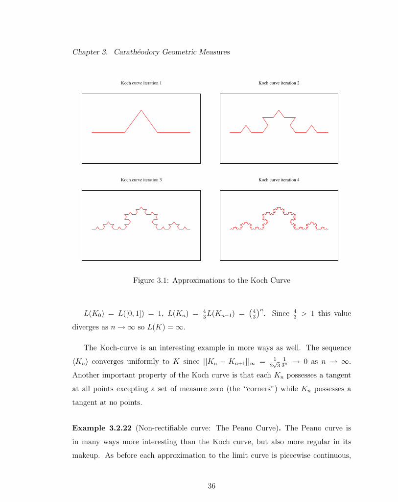
Figure 3.1: Approximations to the Koch Curve

L(K0) = L([0, 1]) = 1, L(Kn) = 43L(Kn−1) =

(43

)n. Since 4

3> 1 this value

diverges as n→∞ so L(K) =∞.

The Koch-curve is an interesting example in more ways as well. The sequence

〈Kn〉 converges uniformly to K since ||Kn − Kn+1||∞ = 12√

313n → 0 as n → ∞.

Another important property of the Koch curve is that each Kn possesses a tangent

at all points excepting a set of measure zero (the “corners”) while Kn possesses a

tangent at no points.

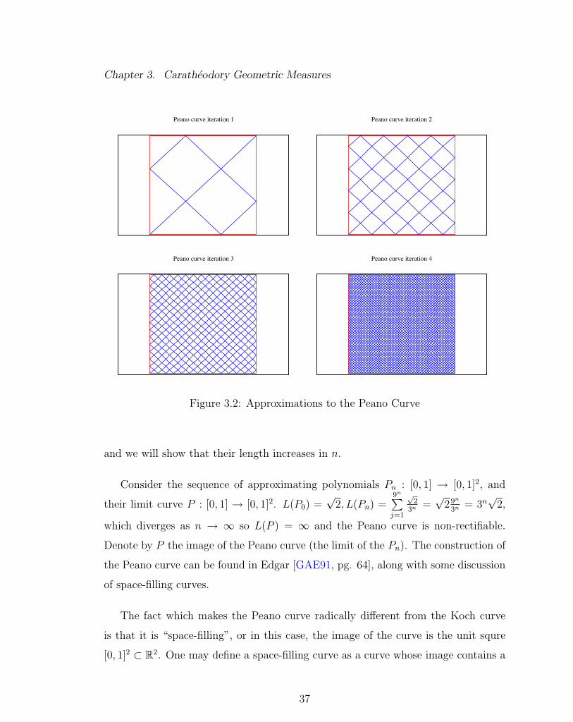
Example 3.2.22 (Non-rectifiable curve: The Peano Curve). The Peano curve is

in many ways more interesting than the Koch curve, but also more regular in its

makeup. As before each approximation to the limit curve is piecewise continuous,

36


Figure 3.2: Approximations to the Peano Curve

and we will show that their length increases in n.

Consider the sequence of approximating polynomials Pn : [0, 1] → [0, 1]2, and

their limit curve P : [0, 1] → [0, 1]2. L(P0) =√

2, L(Pn) =9n∑j=1

√2

3n =√

29n

3n = 3n√

2,

which diverges as n → ∞ so L(P ) = ∞ and the Peano curve is non-rectifiable.

Denote by P the image of the Peano curve (the limit of the Pn). The construction of

the Peano curve can be found in Edgar [GAE91, pg. 64], along with some discussion

of space-filling curves.

The fact which makes the Peano curve radically different from the Koch curve

is that it is “space-filling”, or in this case, the image of the curve is the unit squre

[0, 1]2 ⊂ R2. One may define a space-filling curve as a curve whose image contains a

37


ball B(x, δ) for some x in the image and some δ > 0.

Claim. The image of P , denoted by Γ, is dense in [0, 1]2.

Proof of Claim. We denote the image of Pi by Γi. Consider [0, 1]2. First observe

that Γ0 is simply the diagonal of the square, the maximum distance from any point

in [0, 1]2 to Γ0 is√

22

. More generally, given a square of side ` the maximum distance

of any point a in that square to its diagonal is√

22`. If one subdivides the unit square

into 9n sub-squares in the obvious way (by dividing each side into 3n equal lengths),

we notice that Γn, the nth iteration of the Peano curve, subdivides each of these

squares by the diagonal, and thus the maximum distance from any point in [0, 1]2 to

the nth iteration of the Peano curve Γn is√

22

3−n. Since 3−n → 0 as n → ∞ we see

that the limit Γ is dense in the unit square.

Claim. Γ = [0, 1]2.

Proof of Claim. Let p ∈ [0, 1]2. Then there exists a sequence 〈pn〉 ⊂ Γ such that

pn → p as n→∞. Taking the pre-image of the sequence tn = P−1(pn), we generate

a sequence in [0, 1]. Since [0, 1] is compact, the sequence 〈tn〉 contains a convergent

subsequence, also denoted 〈tn〉, such that tn → t ∈ [0, 1] as n → ∞. Since any

subsequence of a convergent sequence also converges, and by the continuity of P, the

image of 〈tn〉 converges to P (t) = p in [0, 1]2. Thus Γ = [0, 1]2.

Since Γ = [0, 1]2, it contains a ball around any interior point of [0, 1]2, an impor-

tant detail later.

The following lemma foreshadows the result described in Theorem 3.2.25 but is

important for classification of H1 specifically.

Lemma 3.2.23. H1(A) = L1(A) for all A ⊆ R.

38


Proof. The result follows from the same reasoning as in Theorem 3.2.2.

First we observe that both the Lebesgue outer-measure (recall Example 3.1.16)

and the Hausdorff outer-measure are the result of the Caratheodory construction

with differing functions (V (·) and d(·)1 resp.) and sets ({[a, b) ⊆ R : a, b ∈ R, a < b}

and P(R) resp.).

In the special case of R1 the functions V and d agree on the family of sets used

to construct the Lebesgue measure (i.e. V ([a, b)) = d([a, b))1 = b − a). So given

a δ-cover {Ui} of a set A ⊆ R we may replace each element of the cover with a

closed interval of the same diameter which remains a cover (i.e. Ui ⊆ [ai, bi] with

ai = inf Ui, bi = supUi and d(Ui) = d([ai, bi]) = d([ai, bi)) ). Thus we may restrict

ourselves to half-open intervals in the construction of the Hausdorff outer-measure

and H1 = L1.

Theorem 3.2.24. Let ψ : [0, `]→ Rn be a rectifiable curve, and let Γ = ψ([0, `]) be

the image of ψ then H1(Γ) = L(Γ), the arc-length of Γ.

Proof. First we let 0 = a0, . . . , aN = ` be a finite dissection of [0, `], and let Γ0

be the piecewise linear approximation of Γ defined by the dissection. Then Γ0 =

Γ(1)0 ∪ · · · ∪ Γ

(N)0 where Γ

(j)0 , j = 1, . . . , N are the line segments connecting aj−1 and

aj. Let 0 ≤ i < j ≤ N , we note that Γ(i)0 ∩ Γ

(j)0 =

∅ j − i 6= 1

{aj} j − i = 1

We will show that L(Γ0) = H1(Γ0).

Claim. ||ψ(aj)− ψ(aj−1)|| = H1(Γ(j)0 )

Proof of Claim. ||ψ(aj) − ψ(aj−1)|| = ||Tj(ψ(aj) − ψ(aj−1))|| where Tj ∈ O(n,R)

such that Tj(ψ(aj)−ψ(aj−1)) = (αj 0 · · · 0)T ∈ Rn. Then we have Tj(Γ(j)0 ) = [0, αj]

then by Corollary 3.2.9 and Lemma 3.2.23 we have

39


Hs(Γ(j)0 ) = H1(Tj(Γ

(j)0 ))

= H1([0, αj])

= L1([0, αj])

= αj

= ||Tj(ψ(aj)− ψ(aj−1))||

= ||ψ(aj)− ψ(aj−1)||

Claim. H1(Γ0) =N∑j=1

H1(Γ(j)0 )

Proof of Claim. We begin by recalling that an outer-measure ν becomes a measure

when restricted to a σ-algebra of ν-measurable sets. Since, as noted above, Jordan

curves are Borel sets, and by Corollary 3.1.9 we have that H1 is a measure (and thus

is additive) on Borel sets.

Γ0 =N⋃j=1

Γ(j)0 =

(N⋃j=1

Γ(j)0 \ ({aj−1} ∪ {aj})

)∪

N⋃j=0

{aj}

This is essentially the fact that the Γ(j)0 are disjoint except for the endpoints, a

set of measure zero. Removing them from the sum does not change the sum (by

Lemma 3.2.13) so we have

H1(Γ0) = H1

(N⋃j=1

Γ(j)0

)=

N∑j=1

H1(Γ(j)0 )

40


Since all rectifiable curves Γ are the limit points of piecewise linear approximations

Γ0, and H1(Γ0) = L(Γ0) on all such approximations we have H1(Γ) = L(Γ) for all

rectifiable curves.

While we are only considering curves in Rn it has been suggested by Mat-

tila [PM95, pg. 56] that one may choose to use H1 as a definition of the arc-length

of the image of a Jordan curve in an appropriate metric space where the Hausdorff

outer-measures have been defined.

Theorem 3.2.25. For n ∈ N, there exists a constant c(n), dependent only on the

dimension n, such that Hn = c(n)Ln.

This theorem is proved, and the exact constants c(n), are discussed in great

detail in Evans and Gariepy [LCERFG92, pg. 65] and rely upon the isoperimetric

inequality. A beautiful proof of the isoperimetric inequality based upon harmonic

analysis may be found in Stein and Shakarchi [EMSRS03, pg. 103].

Since the Lebesgue measure and Hausdorff outer-measure agree to within a con-

stant for integral dimensions we may normalize the Hausdorff measure to agree ex-

actly with the Lebesgue measure in integral dimensions. Since outer-measures (or

measures) form a vector space over Rn scaling by c(n) is well defined. Often this

normalization is ignored as the actual measure of a set is unimportant in many cases,

and extremely hard to calculate in most cases. As such we are often interested in

the Hausdorff dimension of a set rather than its measure.

Most importantly, the fact that higher dimensional Hausdorff and Lebesgue mea-

sures agree to within a constant that may be normalized away means that the Haus-

dorff measures capture “higher dimensional analogs of length” such as area, volume,

etc. Thus the integral dimensional Hausdorff measures have a well-understood mean-

41


ing and the non-integral dimensional Hausdorff measures may be viewed as a means

of interpolating between the Lebesgue measures.

3.2.3 Generalized Hausdorff Measures

The use of the function ζs(·) = d(·)s in the Caratheodory construction of the Haus-

dorff outer-measures may be made more general by considering the following class of

functions. Let φ be Hausdorff then using F = P(X), as in the standard Hausdorff

measures, we arrive at a different measure ψ(F , φ).

Definition 3.2.26. The Generalized Hausdorff outer-measure with respect to φ is

the following result of the Caratheodory construction: Hφ(A) = limδ↓0

inf∑i

φ(Ui).

Often the φ used is actually a composition of some Hausdorff φ with ζs (i.e.

φ = φ ◦ ζs). Since ζs is Hausdorff by Lemma 2.1.5, φ is Hausdorff.

This notation is intimately related to that which will be used in the later discus-

sion of the Packing Measure.

3.3 Spherical Outer-Measures

This section is included for reasons of completeness and provides upper and lower

bounds on the s-dimensional Hausdorff outer-measure in terms of the so-called s-

dimensional “Spherical-measures”, which too are the result of the Caratheodory

construction.

Definition 3.3.1. Let F = {B(xi, r) : r > 0, xi ∈ X}, and let ζs = d(·)s as in

the construction of the Hausdorff measures. We denote by Ss the result of the

Caratheodory construction from ζ on F (i.e. Ss = ψ(F , ζs)).

42


It should be noted that Federer [HF69, pg. 171] chooses closed balls instead of

open in his definition of F but arrives at the same inequalities below.

Theorem 3.3.2. For all A ⊆ X and 0 < s <∞ the following inequalities hold:

Hs(A) ≤ Ss(A) ≤ 2sHs(A)

Proof. The first inequality is by Lemma 3.2.11 while the second must be shown.

Fix A ⊆ X. Let {Ui} be a δ-cover of A such that δi = d(Ui), then {B(ui, δi) :

ui ∈ Ui} is a (2δ)-cover of A by Lemma 2.2.16.

2sHs(A)def= 2s lim

δ↓0inf∑i

d(Ui)s

= limδ↓0

inf∑i

(2d(Ui))s

≥ limδ↓0

inf∑i

d(B(ui, δi))s

= Ss(A)

Note that the equality after bringing 2s inside the sum makes the infimum effec-

tively over (2δ)-covers of A, and the inequality follows by definition of infimum since

covers by balls are a subset of all possible covers. Since the above is independent of

A the result is proved.

It should be noted that the above inequality is not sharp. In an article by Besi-

covitch [ASB28], a subset of the plane is constructed whose 1-dimensional Hausdorff

outer-measure is 1 while its 1-dimensional spherical outer-measure is 2/√

3. The

specific set is a variant on the standard Sierpinski gasket, and is also discussed in

Mattila [PM95, pg. 75]. In the same article by Besicovitch it is stated that the 1-

dimensional spherical and Hausdorff outer-measures agree on certain “regular” sets

43


while on irregular sets we have

H1(A) ≤ S1(A) ≤ 2√3H1(A)

The specific notions of “regularity” to which Besicovitch refers are defined in

terms of “densities of measures”.

3.4 Net Outer-Measures

The so-called “Net outer-measures” provide “nice” bounds (in that they are in terms

of the dimension of the ambient space only) on the Hausdorff outer-measures in that

the covering sets are well behaved, as we see in Lemma 3.4.4. In fact, the results

proven here are analogous to those proven about the spherical outer-measures in

Section 3.3.

Definition 3.4.1. A net of sets is a family of sets F such that if U,U ′ ∈ F then

U ∩U ′ = ∅ or U ⊆ U ′ or U ′ ⊆ U and each element of F is contained in finitely many

others.

Some authors refer to “nets of sets” as “meshes”, which while more intuitive, has

fallen out of favor in more recent works.

Definition 3.4.2. The dyadic cubes in Rn is the family of sets

F = {[2−jk1, 2−j(k1 + 1))× · · · × [2−jkn, 2

−j(kn + 1)) : ki ∈ Z, j ∈ N}

Lemma 3.4.3. The dyadic cubes are a net of sets.

Proof. The dyadic cubes of side 2−m for all fixed m ∈ N partition Rn and are

pairwise disjoint by construction. Given a dyadic cube of side 2−m it may be uniquely

decomposed into a finite union of 2n dyadic cubes of size 2−(m+1), thus a given dyadic

44


cube of side 2−m is contained in m − 1 dyadic cubes, each being a cube of size 2−`

for ` = 1, . . . ,m− 1.

Lemma 3.4.4. Given an arbitrary sub-family F ′ ( F where F is the dyadic cubes in

Rn, there exists a pairwise disjoint subcollection F ⊆ F ′ such that⋃

F ′i∈F ′F ′i =

⋃Fi∈ eF Fi

Proof. By construction dyadic cubes of the same size are either disjoint or equal. We

inductively define a sub-family of sets

F1 = {F ′ ∈ F ′ : F ′ is of side 2−1}

Fm = {F ′ ∈ F ′ : F ′ is of side 2−m, F ′ ∩ Fj = ∅ for all Fj ∈⋃

1≤j<m

Fj}

Each Fi is a pairwise disjoint collection of dyadic cubes, each of which is not

contained in a larger dyadic cube in F ′. The first property is by definition of the

dyadic cubes while the second is by construction. We then define F =⋃i∈NFi.

The same result is true of any net of sets but the dyadic cubes provide a tangible

context in which to prove the result.

Definition 3.4.5. The s-dimensional Net Outer-Measures, N s are the result of the

Caratheodory construction with F being the dyadic cubes and ζs(·) = d(·)s.

Theorem 3.4.6. For all A ⊆ Rn, n ≥ 2 the following inequalities hold:

Hn(A) ≤ N n(A) ≤ 4nnn/2Hn(A)

Proof. As in the proof of the bounds for spherical outer-measures the first inequality

is by the definition of the Hausdorff outer-measures as shown in Lemma 3.2.11.

To prove the second inequality we start as in the proof of the Spherical measures:

4nnn/2Hn(A) = limδ↓0

inf∑i

(4√n · d(Ui)

)n ≥ limδ↓0

inf∑i

d(Di)n = N n(A)

45


where Di is a δ-cover of Dyadic cubes.

The inequality above requires explanation: given a δ√n-cover of A, we may replace

each element of the cover with 4n dyadic cubes whose diameters are 2−k for appropri-

ate k ∈ N, since for every 0 < δ < 1 there exists k ∈ N such that 2−k−1 < δ√n≤ 2−k.

But, once fixed, those dyadic cubes may not satisfy the infimum over all possible

covers by dyadic cubes of diameter less that δ√n, hence the inequality.

This bound is similar to the result for spherical outer-measures above (in fact, the

parallel is the reason for the discussion of spherical measures). In and of themselves,

neither of these families of outer-measures provides terribly more information than

the Hausdorff outer-measures do, but due to their use of more tractable sets, they are

useful in computation of the measures of sets. Moreover, they provide information

about the “Hausdorff dimension” of a given set, as we will see shortly.

46

Chapter 4

Packing Outer-Measures

Our next focus, the packing outer-measures, provide natural lower-bounds for sets

where the Hausdorff outer-measures provide natural upper-bounds. They are not

derived from the Caratheodory construction above, but instead are constructed from

an apparently “dual” construction of packings rather than coverings. In this section

we follow the general construction of McClure [MM94] in his Dissertation work. As

in the case of Hausdorff outer-measures there is a family of packing outer-measures

parameterized by s ∈ [0,∞), each of which provides a meaningful measure for a

restricted family of sets.

Definition 4.0.7. Let (X, d) be a metric space, A ⊆ X. A centered δ-packing of

A is a collection {B(ai, δi)} of disjoint closed balls centered about ai ∈ A of radius

δi ≤ δ.

Lemma 4.0.8. Let (X, d) be a metric space where d(B(x, r)) = d(B(x, r)) and

A ⊂ X. Fix δ > 0. Let {B(ai, δi)} be a collection of disjoint open balls centered

about ai ∈ A with radius δi < δ. This collection of disjoint open balls is the limit

point of a sequence of centered δ-packings consisting only of closed balls (as in the

definition above).

47

Chapter 4. Packing Outer-Measures

Proof. limj→∞

B(ai, δi − 1/j) = B(ai, δi). Note that we want 1/j < δi which is always

true in the limit. Moreover, since B(ai, δi − 1/j) ( B(ai, δi) and the collection

{B(ai, δi)} is pairwise disjoint the collection {B(ai, δi−1/j)} is a centered δ-packing

as in the first definition.

This lemma shows that in a given metric space where closed balls and open balls

of the same radius are of the same diameter we may use either open or closed packings

for our centered δ-packings. This is the case in Rn, so in instances where the use of

open balls is advantageous we are free to consider such packings.

Definition 4.0.9. Let B be centered δ-packing of a set A ⊆ X. A centered δ-packing

B′ of A is called an extension of B if B ( B′.

Lemma 4.0.10. Let φ be Hausdorff. Let B = {B(ai, δi)} be a centered δ-packing of

A ⊆ X, and B′ = {B(a′i, δ′i)} be an extension of B, then

∑i

φ(2δi) <∑i

φ(2δ′i).

Proof. Let B = {B(ai, δi)}i∈I and by definition of extension B′ = B ∪ {B(a′i, δ′i)}i∈I′

where I, I ′ are countable index sets. Then∑i∈I

φ(2δi) <∑i∈I

φ(2δi) +∑i∈I′

φ(2δ′i) =∑i∈I∪I′

φ(2δ′i)

The first inequality follows from φ being Hausdorff (and thus positive), and the

second equality is by the construction of B′.

Definition 4.0.11. Let (X, d) be a metric space, φ Hausdorff. We define the Packing

pre-measure by

P φδ (A)

def= sup

{∑i

φ(2δi) : {B(ai, δi)} a centered δ-packing of A

}

Note. In much of the literature we find the definitions of the Packing outer-measures

P s constructed of φs(A) = d(A)s for s ∈ [0,∞). This has technical problems in

48


notation so often authors choose a “radius definition” where instead of φs(B(x, δ)) =

d(B(x, δ))s we find φs(B(x, δ)) = (2δ)s where δ is the radius of a closed ball in a

given δ-packing of A. These pre-measures and associated outer-measures (defined

below) are denoted by P s and Ps respectively, where it is to be understood that

the superscript s ∈ [0,∞) is associated to φs. The case s = 0 is used by making

the assumption that 00 = 0 and t0 = 1 for t 6= 0. By choosing a more complicated

function φs(2δi) we generate more complicated outer-measures in a similar manner

to the Generalized Hausdorff outer-measures above. This is the distinction made by

McClure, as noted in the introduction to this section, which we follow here.

Notation. As in the Caratheodory construction we will, for brevity, write P φ(A) =

sup∑i

φ(2δi) where the {δi} being summed over are understood to come from a

centered δ-packing {B(ai, δi)} of A.

As in the case of the outer-measures constructed via the Caratheodory construc-

tion we now consider the limiting behavior of the approximating size δ packing

pre-measures.

Definition 4.0.12. Let A ⊆ X then P φ(A)def= lim

δ↓0P φδ (A).

Lemma 4.0.13. P φδ is non-decreasing in δ

Proof. Fix A ⊆ X. Define Sδ(A) ={{B(ai, δi)} a centered δ-packing of A

}and

Sδ(A) =

{∑i

φ(2δi) : {B(ai, δi)} ∈ Sδ(A)

}.

Let 0 < δ0 < δ1 then Sδ0(A) ⊂ Sδ1(A) and thus Sδ0(A) ⊂ Sδ1(A). We then have

P φδ0

(A) = sup Sδ0(A) ≤ sup Sδ1(A) = P φδ1

(A).

Since the inequality is independent of A we see that P φδ is non-decreasing in δ.

Corollary 4.0.14. P φ(A) = infδ>0

P φδ (A).

Proof. Proof is analogous to the proof of Lemma 3.1.5.

49


It is clear that P φ(∅) = 0 since there are no centered δ-packings of the empty

set. To show monotonicity of P φ, notice that given sets A ⊆ A′ ⊆ X, any centered

δ-packing of A is also a centered δ-packing of A′, so taking the appropriate suprema

we find that P φ is monotonic. Though these results are promising the packing pre-

measure has one major flaw, P φ is not subadditive!

Lemma 4.0.15. P φ is finitely subadditive.

Proof. Let A,A′ ⊆ X. Every packing of A∪A′ may be partitioned into two packings

of A and A′ repectively but not every packing of general A,A′ may be derived this

way (consider the case when A ∩ A′ is non-trivial). Let {B(ai, δi)} be a packing of

A ∪ A′, then the partition the packing such that {B(a′i, δi)} is a packing of A′ (i.e.

a′i ∈ A′), and similarly for A.

Lemma 4.0.16. P φ is not countably subadditive.

Proof. Proof by example: we consider the packing outer-measure of N ⊂ R with

respect to the Euclidean metric on R and claim P φ(N) >∞∑i=0

P φ({i}).

First we note that the packing outer-measure of a singleton is zero

P φ({i}) = infδ>0

P φδ ({i})

= infδ>0

sup∑i

φ(2δi)

= infδ>0

supφ(2δi)

= infδ>0

φ(2δ) = 0

where the final equality is by the Hausdorff property of φ. Thus we have

∞∑i=0

P φ({i}) = 0

50


On the other hand

P φ(N) = infδ>0

P φδ (N) = inf

δ>0sup

∞∑i=0

φ(2δ) = infδ>0

φ(2δ) sup∞∑i=0

1 =∞

The above divergence of the packing outer-measure holds for all δ > 0 so the

infimum is also infinite.

Thus we have P φ(N) >∞∑i=0

P φ({i}).

There are also compact examples of sets whose packing pre-measures dominate

their packing outer-measure. For example {1/n : n ∈ N}.

Definition 4.0.17. The φ-induced packing outer-measure of A is defined as

Pφ(A) = inf

{∑i

P φ(Ai) : A =⋃i

Ai

}

This definition is very similar to the definition found in Halmos [PH64, pg. 42]

in defining the extension of a measure to an outer-measure. Notice that this defini-

tion fixes the above problem of infinite subadditivity failing since simply taking the

singleton decomposition of the naturals makes Pφ(N) = 0.

Lemma 4.0.18. Every countable set A is of measure zero with respect to the Packing

outer-measures.

Proof. Take as a cover of A the collection of singletons making up A. Their respective

packing pre-measures is zero, so the sum of their pre-measures is zero, so their

Packing measure is zero.

Lemma 4.0.19. P0 is the counting measure.

Note that in this case both P 0 and P0 are the packing pre-measure and outer-

measure associated to the function φ0(·) = d(·)0 with the assumption that 00 = 0.

51


Proof. The proof that P 0 is the counting measure is almost identical to the proof that

H0 is the counting measure in Lemma 3.2.17. To prove that P0 is also the counting

measure, consider a set A and any collection {Ai} such that A =⋃i

Ai. As we will see

shortly (in Lemma 4.0.21), P0(A) ≤ P 0(A) so we need P 0(A) ≤ P0(A). One need

only note that P 0(A) ≤∑i

P 0(Ai) for any cover of A, thus P 0(A) ≤ inf∑i

P 0(Ai) =

P0(A). Thus P0 is the counting measure.

Lemma 4.0.20. Let A ⊆ X. An equivalent definition of the packing outer-measure

is

Pφ(A) = inf

{∑i

P φ(Ai) : A ⊆⋃i

Ai

}

Proof. Since P φ is monotonic we know that P φ(A∩Ai) ≤ P φ(Ai). Let {Ai} be such

that A ⊆⋃i

Ai then∑i

P φ(A ∩ Ai) ≤∑i

P φ(Ai), independent of the specific cover

{Ai} chosen. Moreover every partition of the form A =⋃i

Ai is also of the form

A ⊆⋃i

Ai, and the result follows.

This equivalent definition is found in Hasse [HH86], where it is the only definition.

Lemma 4.0.21. Let A ⊆ X. Pφ(A) ≤ P φ(A).

Proof. Notice that in the definition of Pφ we take infimum over all coverings {Ai}

of A such that A =⋃i

Ai, and as such A is a covering of itself, thus the result

follows.

Theorem 4.0.22. Pφ is an outer-measure.

Proof.

• Since P φ(∅) = 0 and Pφ(∅) ≤ P φ(∅) = 0 we have Pφ(∅) = 0.

52


• (Monotonicity) Let A ⊆ A′ ⊆ X then any centered δ-packing {Ui} of A is also a

centered δ-packing of A′ so we have P φ(A) ≤ P φ(A′). Moreover, every partition

of A′ induces a partition of A. Given a partition of A′ =⋃iA′i the induced

partition of A is A =⋃iAi, where Ai = (A′i ∩ A). Thus Ai ⊆ A′i and by the

monotonicity of P φ we have Pφ(A) = inf

{∑i

P φ(Ai)

}≤ inf

{∑i

P φ(A′i)

}=

Pφ(A′).

• (Countable sub-additivity) Let {Ai} ⊂P(X). Define the following sets:

U =

{{Ui} :

⋃i

Ai =⋃i

Ui

}

V (i) =

{{V (i)

j } : Ai =⋃j

V(i)j

}

W =

{⋃i

{V (i)j } : {V (i)

j } ∈ V (i)

}

U is the set of all covers of⋃i

Ai, each V (i) is the set of all covers of Ai, and

W is the set of all covers of⋃i

Ai constructed of unions of all covers of the

individual Ai as defined in V (i).

Claim. W ( U .

Proof of Claim. Let {Wi} ∈ W then {Wi} =⋃k

{V (k)j } where Ak =

⋃j

V(k)j .⋃

i

Wi =⋃j

⋃k

V(k)j =

⋃k

⋃j

V(k)j =

⋃k

Ak thus {Wi} ∈ U so W ⊂ U . Now to see

that every cover of⋃i

Ai is not in W , simply consider A1, A2 ∈ P(X) such

that d(A1, A2) > 0 and a partition {U1, U2} of A1 ∪ A2 such that Ui ∩ Aj 6= ∅

for i, j = 1, 2, and A1 ∪ A2 = U1 ∪ U2. Then neither Uj can be in either V (i)

for i, j = 1, 2.

53


With that small technicality the result follows.

Pφ(⋃i

Ai)def= inf

{∑i

P φ(Ui) : {Ui} ∈ U

}

≤ inf

{∑i

P φ(Wi) : {Wi} ∈ W

}

= inf

{∑j

∑k

P φ(V(j)k ) : {V (j)

k } ∈ V(j)

}

=∑j

inf

{∑k

P φ(V(j)k ) : {V (j)

k } ∈ V(j)

}=∑j

Pφ(Aj)

The inequality follows from the fact that the infimum in the latter set is taken

over a smaller set (i.e. W ( U). The following equality follows from the fact

that since P φ is positive re-ordering the summands does not change the value

of the series. The next equality is due to the fact that the infimum is taken

over covers from a fixed V (j) which are completely independent at each stage of

the sum. The final equality is simply by the definition of the packing measure.

Lemma 4.0.23. Pφ is translationally invariant over Rn.

Proof. Let A ⊂ Rn. If {B(ai, δi)} is a δ-packing of A then {B(ai + x, δi)} is a δ-

packing of A + x. Since translation of a packing does not change the radii of the

closed balls in the packing the result follows.

Lemma 4.0.24. Pφ is metric and Borel.

Proof. By Caratheodory’s Criterion (Theorem 2.3.9) it is enough to show that Pφ

is metric. Let A,A′ ⊂ X such that d(A,A′) ≥ δ > 0 Then for all δ3-packings of A

(resp. A′) no element of the packing intersects A′ (resp. A).

54


Thus, given a δ3-packing {Vi} of A ∪ A′, we may partition the packing into two

packings {Ui} and {U ′i} where {Ui : Ui = B(ai, δi), ai ∈ A} (and similarly for A′

define {U ′i : U ′i = B(a′i, δ′i, }). Then we have {Vi} = {Ui} ∪ {U ′i}. So following the

definitions we have

P φ(A ∪ A′) = limδ↓0

sup

{∑i

φ(2δi) : {B(ai, δi)}

}

= limδ↓0

sup

{(∑i

φ(2δi)

)+

(∑i

φ(2δ′i)

)}= lim

δ↓0sup

∑i

φ(2δi) + limδ↓0

sup∑i

φ(2δ′i)

= P φ(A) + P φ(A′)

Thus P φ is metric.

Let {Ai} be a partition of A∪A′, then we define A(1)i = Ai∩A and A

(2)i = Ai∩A′,

then Ai = A(1)i ∪A

(2)i so {Ai} = {A(1)

i ∪A(2)i }. Since P φ is metric we have P φ(Ai) =

P φ(A(1)i ∪ A

(2)i ) = P φ(A

(1)i ) + P φ(A

(2)i ) since d(A

(1)i , A

(2)j ) > 0 for all i, j ∈ N.

So since every partition of A (resp. A′) can be obtained from the restriction of a

partition of A ∪ A′ in the above way we have

Pφ(A ∪ A′) = inf

{∑i

P φ(Ai) : A ∪ A′ =⋃i

Ai

}

= inf

{∑i

(P φ(A(1)i ) + P φ(A

(2)i ))

}

= inf

{(∑i

P φ(A(1)i )

)+

(∑i

P φ(A(2)i )

)}

= inf

{∑i

P φ(A(1)i )

}+ inf

{∑i

P φ(A(2)i )

}= Pφ(A) + Pφ(A′)

55


So Pφ is metric, and thus by Caratheodory’s Criterion Pφ is Borel.

We now roughly follow the opening notes of Edgar [GAE94] and the proper-

ties listed in Hasse [HH86] and discuss in detail certain properties of the Packing

outer-measure (and pre-measures). The difference being that Edgar only explicitly

discusses Ps instead of Pφ, where as Hasse discusses the topic in generality using

different notation.

Lemma 4.0.25. Finite packings suffice in the following sense:

P φδ (A) = sup

M∈N

{M∑i=1

φ(2δi) : {B(ai, δi)}Mi=1 a finite δ-packing of A

}

One must be careful to interpret this lemma correctly. It does not say that

given a set A there exists a finite δ-packing B = {B(ai, δi)}Mi=1 of A such that

P φδ (A) =

M∑i=1

φ(2δi) for some fixed finite M . Instead it means that if P φδ (A) is finite

then one may arbitrarily estimate its value by a finite sum.

Proof. If A does not admit an infinite packing (for example #A < ∞) then the

lemma is clear so we assume A admits an infinite packing. If A admits a countably

infinite centered δ-packing B = {B(ai, δi)} then it may be enumerated. Then since

limj→∞

j∑i=1

φ(2δi) =∞∑i=1

φ(2δi) we have supj

j∑i=1

φ(2δi) =∞∑i=1

φ(2δi) since the finite sum

strictly increases in j. So we have

supM∈N

{M∑i=1

φ(2δi) : {B(ai, δi)}Mi=1 a finite δ-packing of A

}= sup

∑i

φ(2δi)

And the result is proved.

Lemma 4.0.26. Let A ⊆ Rn, then Pφ(A) = Pφ(A).

Proof. Let {B(ai, δi)} be a centered δ-packing of A. If ai ∈ A \A then there exists a

sequence 〈a(j)〉 such that a(j) → ai as j →∞ by definition of closure. Thus we may

56


replace B(ai, δi) in the packing with B(a(j), δ(j)) such that for any ε, d(ai, a(j)) < ε

and thus φ(2δi)− φ(2δ(j)) < ε since φ is Hausdorff.

So any δ-packing of A may be arbitrarily approximated by a δ-packing of A, thus

P φ(A) = P φ(A). Since every collection {Ai} such that A ⊆⋃i

may be seen as being

induced by a similar cover of A the result holds for Pφ.

One should note that we use the continuity of φ to guarantee that

φ(2δi)− φ(2δ(j)) < ε

in the above proof!

Corollary 4.0.27. Let A ⊆ Rn. Since P φ(A) = P φ(A) we may take the definition

of Pφ as

Pφ(A) = inf

{∑i

P φ(Ai) : A ⊆⋃i

Ai, Ai Borel

}

Corollary 4.0.28. Pφ is Borel-regular in Rn.

Proof. Since given A ⊆ X, by definition A is closed, and thus Borel, by the last

lemma Pφ is Borel-regular.

One should note that our decision to limit ourselves to Rn is motivated by the

opening notes in Joyce’s paper describing a space on which a certain class of packing

measures is not Borel-regular [HJ99]. Moreover his opening prose discuss a number

of issues which may arise in non-Euclidean spaces or with weak definitions of our

function φ.

57


4.1 A “Dual” Construction?

If one were able to generate a family of packing outer-measures in much the same way

we generate geometric outer-measures using the Caratheodory construction, there

would be a satisfying symmetry in the theory. Let us pursue such a construction and

what would be necessary for it to be valid.

In the Caratheodory construction one requires a family of sets F ⊆ P(Rn) (we

will restrict ourselves in this discussion to Rn), and a function ζ : F → [0,∞) with

appropriate properties. In the explicit construction of the Packing outer-measures

one uses packings of balls centered about points in a given set. We consider packings

of a set A ⊆ Rn. We may set F = {B(ai, δ), δ ∈ (0,∞))} but this set is dependent

upon the set being packed so instead we denote it FA. If instead we replace FAwith F = {B(x, δ) : x ∈ Rn, δ ∈ (0,∞)}, the set of all centered δ-packings of

Rn, this set is not dependent upon that being packed but it is fairly unmanageable

and FA ⊆ F . Taking motivation from the separability of the space one may wish

to consider packings from the sets FQ = {B(x, δ), x ∈ Qn, δ ∈ (0,∞)} or even

F2 = {B(x, δ) : x ∈ Qn, x = a/2n, a ∈ Z, δ ∈ (0,∞)} since both Qn and the dyadic

rationals, {x ∈ Qn, x = a/2n, a ∈ Z}, are countable and dense in Rn. This yields

little since the constructed packing using either family of sets measures Rn \ Qn as

zero. Moreover, we can take any set, remove the rational points, and the resulting

set has a maximal packing of size zero!

One may also want to generate basic bounded relations using easier to calculate

packings similarly to what was done with the net outer-measures above. To do so one

needs to consider packings by some net of sets. The dyadic cubes seem a reasonable

candidate if we consider “centered dyadic cubes”, since each dyadic cube has a center

point that is also a dyadic rational. We immediately run into the problem above that

not every set contains a dyadic rational (or even a rational at all)!

58


Thus we find that there is no clear construction, “dual” to the Caratheodory

construction, for packing outer-measures in Rn, or any other metric space.

59

Chapter 5

Dimension Theory

5.1 Hausdorff Dimension

The following theorem has many equivalent statements:

Theorem 5.1.1. Let s, t ∈ R such that 0 ≤ s < t <∞ then for any A ⊆ X we have

Hs(A) <∞ implies Ht(A) = 0. Equivalently Ht(A) > 0 implies Hs(A) =∞.

Proof. The following is the standard proof as found in Falconer [KJF85, pg. 7],

Mattila [PM95, Theorem 4.7, pg. 58], and Evans and Gariepy [LCERFG92, Lemma

2, pg. 65]:

Let 0 < s < t, then we have Hsδ(A) ≥ Ht

δ(A) ≥ δs−tHtδ(A) where the first

inequality is by by Lemma 3.2.10 and the final inequality is from the assumption

that 0 < δ < 1 and thus 0 < δs−t < 1.

So we have Hs(A)def= lim

δ↓0Hsδ(A) ≥ lim

δ↓01

δt−sHtδ(A) =

0 if Htδ(A) = 0

∞ if Htδ(A) > 0

60

Chapter 5. Dimension Theory

This theorem may be re-phrased as follows:

Theorem 5.1.2. Let A ⊂ X. There exists a unique s ∈ [0,∞) such that Ht(A) =∞

if t < s and Ht(A) = 0 if t > s.

Definition 5.1.3. The Hausdorff Dimension (or Hausdorff-Besicovitch Dimension)

of a set A is the unique s ∈ [0,∞) such that

Ht(A) =

∞ for all 0 ≤ t < s

0 for all t > s

Notation. We denote the Hausdorff Dimension of a set A by dimH(A).

Corollary 5.1.4. If A ⊆ X and dimH(A) = s then Ht(A) = 0 for all t > s, and

Ht(A) =∞ for t < s.

Notice that this is merely a re-statement of Theorem 5.1.1 in terms of “Hausdorff

dimension”.

Lemma 5.1.5. Let A ⊆ X, then the following equalities are true:

dimH(A) = sup{s : Hs(A) > 0} = sup{s : Hs(A) =∞}

= inf{s : Hs(A) <∞} = inf{s : Hs(A) = 0}

Proof. Since dimH(A) = s is the unique number such that Ht(A) = 0 for all t > s

and Ht(A) =∞ for all t ≤ s all of the equalities hold by definition.

It should be noted that if dimH(A) = t then the specific value of Ht(A) may be

zero, finite, or infinite.

Lemma 5.1.6. dimH is monotonic i.e. if A ⊆ A′ ⊆ X then dimH(A) ≤ dimH(A′).

61


Proof. If dimH(A) = s then we have Hs(A) ≤ Hs(A′) by monotonicity of Hs. If

Hs(A) = ∞ then Hs(A′) = ∞ and thus dimH(A′) ≥ s. If, on the other hand,

Hs(A) = α < ∞, then Hs(A′) is either finite or infinite. If it is infinite then we

are in the previous case, if it is finite then dimH(A′) = s by definition of Hausdorff

dimension.

So dimH is monotonic.

Theorem 5.1.7. Let A ⊆ Rn, Consider L : A → Rm Lipschitz with Lipschitz

constant c, then dimH(L(A)) ≤ dimH(A).

Proof. Let s = dimH(A). Recalling Theorem 3.2.4 we know that Hs(L(A)) ≤

csHs(A) and the result is immediate by the definition of dimH.

And as we saw in Example 3.2.7, strict inequality of dimH under Lipschitz maps

is possible.

Corollary 5.1.8. Hs is not Radon.

Proof. Let A ⊂ X be a compact set such that dimH = t, then if s < t then Hs(A) =

∞ so Hs is not locally finite.

While the definition of Hausdorff dimension and its corollaries provide powerful

machinery, in the theory an explicit calculation is not amiss.

Lemma 5.1.9. Let A be countable then dimH(A) = 0.

Proof. We know that Hs(A) = 0 for all s > 0 by Lemma 3.2.12 and that H0 is the

counting measure by Lemma 3.2.17, so H0(A) > 0, thus zero satisfies the definition

of Hausdorff dimension for A and dimH(A) = 0.

62


Lemma 5.1.10. For s > n > 0,Hn(Rn) =∞,Hs(Rn) = 0. Equivalently dimH(Rn) =

n.

Proof. This proof is by Falconer [KJF85, pg. 8]. Consider the n-dimensional cube

C = [0, 1]n ⊂ Rn. Let δ > 0, then there exists a k ∈ N such that k−1n1/2 < δ.

We may divide C into kn subcubes of size k−1 in the obvious way. Then Hn(C) ≤

kn(k−1n1/2)n = nn/2 <∞. Thus, since s > n and by Theorem 5.1.1 Hs(C) = 0, and

since Rn is a countable union of translated cubes and by the monotonicity of Hs we

have Hs(Rn) = 0 and Hn(Rn) =∞.

Corollary 5.1.11. Hs is σ-finite.

Lemma 5.1.12. Let A = B(x, r) be the open ball of radius r about x ∈ Rn, then

dimH(A) = n.

Proof. By Lemma 3.2.25 we know that 0 < Hn(A) = c(n)Ln(A) < ∞ since A is

bounded, thus Ln(A) <∞, and c(n) is finite. So dimH(A) = n.

Corollary 5.1.13. Let A ⊆ Rn such that for some a0 ∈ A and some r > 0 the ball

B(a0, r) ⊆ A then dimH(A) = n

Proof. By Lemma 5.1.12 we know dimH(B(a0, r)) = n and by Lemmas 5.1.6 and 5.1.10

we know that

n = dimH(B(a0, r)) ≤ dimH(A) ≤ dimH(Rn) = n

as was to be shown.

Corollary 5.1.14. Any space-filling curve in Rn is of Hausdorff dimension n.

Proof. By definition a space-filling curve contains a ball, and by Lemma 5.1.13 we

are done.

63


Corollary 5.1.15. Let A ⊆ R, if 0 < dimH(A) < 1 then A is totally disconnected.

Proof. If A contains an interval (a connected non-singleton subset) then dimH(A) = 1

by Corollary 5.1.13, so A does not possess any non-singleton connected components,

and thus A is totally disconnected.

An interesting feature of the Hausdorff dimension (and subsequently the Haus-

dorff outer-measures indexed by s) is that it partitions the set of Hausdorff-measurable

sets. These sets are precisely those which meet the definition of Caratheodory mea-

surability for some Hs. The partition of these sets is trivial in that two sets are in the

same class in the partition if they are of the same Hausdorff dimension. There are

sets which are not Hausdorff measurable so those sets are excluded in the partition,

and those sets which remain lie in the partition nicely.

Lemma 5.1.16. Let 0 < λ < 1/2 then dimH(C(λ)) = log(2)/ log(1/λ) where C(λ)

is the generalized Cantor set defined in Example 3.2.14.

Proof. This proof is also by Falconer [KJF85, pg. 14], though all details of the

general result for C(λ) are shown where as Falconer only shows the result for C(1/3)

and provides a hint as to the general result.1 This proof is similar to a proof in

Mattila but provides a sharp inequality which thus computes that actual measure

of the Cantor set with respect to the s-dimensional Hausdorff outer-measure (for s

defined below).

By the nature of the Hausdorff outer-measures it is generally easier to bound the

measure of a set from above than below so we begin there. Set s = log(2)/ log(1/λ).

1For the careful reader it should be noted that in the 2002 paperback printing of Fal-coner’s book there is a typo on pg. 15. The author provides a set of inequalities similarto those used here but the second equality shown should be greater-than-or-equal and thelast inequality should be equality.

64


Recalling the construction of C(λ), we begin with I0,1 = [0, 1] then define the

sub-intervals Ij,k and C(λ) =∞⋂k=0

2k⋃j=1

Ik,j. Now we notice that every finite intersection

CM(λ) =M⋂k=0

2k⋃j=1

Ik,j is a finite cover of C(λ) (containing 2k intervals) and Ik,j is an

interval of length λk so, given δ, for sufficiently large M , CM(λ) is a δ-cover of C(λ).

Then, rewriting λk = λ−k0 , 2 < λ0 <∞, we have

Hsλ−k0

(C(λ)) ≤ 2kλ−sk0 = 2k2−k = 1

since λs0 = λlog(2)/ log(λ0)0 = 2 by the properties of the logarithm. So s is an upper-

bound on the Hausdorff dimension of C(λ) since Hs(C(λ)) <∞.

To show that Hs(C(λ)) > 0, and thus s is the Hausdorff dimension of C(λ), we

need to show that 1 ≤∑i

d(Ii)s for any cover of C(λ) by intervals {Ii}.

We begin by noting that since C(λ) is compact, for any cover of open intervals

there is a finite sub-cover {Ij} consisting of open intervals. We then take the closure

of each {Ij} and reduce each interval to make each one the smallest possible interval

containing all of the Ij,k used in the construction of C(λ).

Now let Ij,k, I`,m be two disjoint intervals from the construction of C(λ) (Falconer

refers to these as “net intervals”) contained in Ii (potentially from different iterations

of the construction), then

d(Ii) > d(Ij,k) + d(Ui) + d(I`,m)

where Ui is an open interval in the complement of Ij,k ∪ I`,m contained in Ii. Then if

d(Ij,k) + d(I`,m) ≤ 2d(Ui)λ

1− 2λ

where 1− 2λ is the length removed from the unit interval in the first iteration of the

construction, we get the following string of inequalities:

65


d(Ii)s = (d(Ij,k) + d(Ui) + d(I`,m))s

≥(

1

2λ(d(Ij,k) + d(I`,m))

)s=

(1

λ

)s(d(Ij,k) + d(I`,m)

2

)s= 2

(d(Ij,k) + d(I`,m)

2

)s≥ 2

(1

2d(Ij,k)

s +1

2d(I`,m)s

)= d(Ij,k)

s + d(I`,m)s

The first inequality is by the condition stated before the equations and the second

is by the concavity of f(t) = ts (since a function f is concave down if and only if

f(x+y2

) ≥ f(x)+f(y)2

). Thus we may replace Ii with the two sub-intervals Ij,k and I`,m in

the above sum:∑j

d(Ij)s =

∑j

(d(Ij,k)s + d(I`,m)s). Each time we do this we increase

the number of intervals covering C(λ) by two but the covering set remains finite.

We may repeat this process until each element of this finite covering is of length λj

which then must cover all of the {Ij,`}` thus the sum above must be greater than

2j( 1λj )s = 1.

Thus dimH(C(λ)) = s = log(2)/ log(1/λ).

Corollary 5.1.17. Let 0 < λ < 1/2, C(λ) be the associated Cantor set, and s =

log(2)/ log(1/λ), then Hs(C(λ) = 1.

Proof. In the calculation of the Hausdorff dimension of C(λ) we bound Hs(C(λ))

from both above and below by 1.

Corollary 5.1.18. For every s ∈ [0, 1] there exists a set As ⊆ [0, 1] such that

dimH(As) = s.

66


Proof. We begin with the two boundary conditions s = 0, 1: in the case s = 0 simply

take A0 to be any finite or countable subset of [0, 1], and H0 is the counting measure,

so by combining Lemma 3.2.12 and the definition of Hausdorff outer-measures we

find that dimH(A0) = 0. On the other hand if s = 1 then let A1 = [0, 1], since

H1([0, 1]) = L1([0, 1]) = 1 we see that by definition of the Hausdorff outer-measures

dimH([0, 1]) = 1 and we are done.

We now show that the map λ 7→ log(2)/ log(1/λ) is onto (0, 1). We know that

limλ→0

log(λ) = −∞ so limλ→0

log(2)/ log(1/λ) = limλ→0

log(2)/(− log(λ)) = 0. On the other

hand, limλ→1/2

log(2)/ log(1/λ) = 1 by the continuity of log and by the intermediate

value theorem the function takes on all values between the two limits. In fact, the

map is bijective since the derivative of log is strictly positive on (0,∞).

Since dimH(C(λ)) = log(2)/ log(1/λ) for λ ∈ (0, 1/2) the above argument shows

that there is a Cantor set C(λ) realizing every Hausdorff dimension in (0, 1). More-

over, the bijectivity of above map shows that there is a unique Cantor set realizing

each dimension.

Theorem 5.1.19. Let A,B ⊆ X then dimH(A ∪ B) = max{dimH(A), dimH(B)}

and dimH(A ∩B) ≤ min{dimH(A), dimH(B)}.

Proof. First we set dimH(A) = s and dimH(B) = t, and assume without loss of

generality that s < t. Then Ht(A) = 0 by definition of Hausdorff dimension, and

Ht(B) = β ∈ (0,∞) so we have

β = Ht(B) ≤ Ht(A ∪B) ≤ Ht(A) +Ht(B) = Ht(B) = β

The first inequality is by monotonicity of outer-measures and the second is by

subadditivity. So

dimH(A ∪B) = t = max{dimH(A), dimH(B)} = max{s, t}

67


Similarly to the first half of the proof we have Hs(A) = α and Hs(B) = ∞.

Moreover by definition A ∩B ⊆ A so

0 ≤ Hs(A ∩B) ≤ Hs(A) = α

where the first inequality is by definition and the second is by monotonicity of outer-

measures. Thus we have

dimH(A ∩B) ≤ s = min{dimH(A), dimH(B)} = min{s, t}

Corollary 5.1.20. Let A = {Ai} ⊂ P(X) be countable, then dimH(⋃i

Ai) =

supi

dimH(Ai). Moreover if dimH(X) < ∞ then supi

dimH(Ai) < dimH(X). Finally

0 ≤ dimH(⋂i

Ai) ≤ infi

dimH(Ai).

Proof. By Theorem 5.1.19 that dimH(⋃i

Ai) = supi

dimH(Ai) is clear since dimH

can only increase under union. Any by monotonicity of dimH that supi

dimH(Ai) <

dimH(X) is clear. Actually the moreover condition in the statement holds if dimH(X) =

∞ but the conclusion is then automatic and vacuous.

Finally, since dimH(A) ≥ 0 for all A ⊆ X, and since dimH decreases under

intersections, we have 0 ≤ dimH(⋂i

Ai) ≤ infi

dimH(Ai), so the result is proved.

Theorem 5.1.21. There exists Borel sets A,B ⊂ R of Hausdorff dimension 0 such

that dimH(A×B) > 0.

For a proof please see Falconer [KJF85, pg. 73, Thm. 5.11]. The proof is

constructive and interesting but outside of the scope of this work.

The primary motivation for including the Spherical and Net outer-measures is

that they are “comparable measures”, meaning that they are bounded above and

below by the Hausdorff measures, and thus may be used to analyze the Hausdorff

dimension of a given set with respect to more tractable families of sets.

68


5.2 Packing Dimension

In this section we choose the specific family of packing outer-measures Ps indexed

by a real parameter s ∈ [0,∞) as discussed earlier.

Lemma 5.2.1. P s,Ps are non-increasing in s.

Proof. Let 0 ≤ s < t < ∞, A ⊆ X. First we prove the lemma for the packing

pre-measures.

Since the set of δ-packings of the set A does not vary with s, and thus the pre-

measure being applied to the set we have

P sδ (A)

def= sup

∑i

(2δi)s ≥ sup

∑i

(2δi)t def= P t

δ (A)

But this inequality is independent of δ so we have

P s(A)def= lim

δ↓0P sδ (A) ≥ lim

δ↓0P tδ (A)

def= P t(A)

So P s is non-increasing in s. It follows that we have

Ps(A)def= inf

{∑i

P s(Ai) : A =⋃i

Ai

}≥ inf

{∑i

P t(Ai) : A =⋃i

Ai

}def= P t(A)

The inequality above is because the covers of A are shared between the two

infimums and P s is non-increasing in s so Ps is non-increasing in s.

Just as in the case of the Hausdorff dimension there exists a critical value of s at

which the family of packing outer-measures provides meaningful information about

a given set.

Theorem 5.2.2. Let s, t ∈ R such that 0 ≤ s < t <∞ then for any A ⊆ X we have

P s(A) <∞ implies P t(A) = 0. Equivalently, if P t(A) > 0 implies P s(A) =∞.

69


Proof. This proof is nearly identical to the makeup of the proof of Theorem 5.1.1,

which is an analogous statement about the family of Hausdorff measures.

Let 0 < s < t, then by Lemma 5.2.1 we have P sδ (A) ≥ P t

δ (A) ≥ δs−tP tδ (A)

where the final inequality follows from the assumption that 0 < δ < 1 and thus

0 < δs−t < 1.

So we have P s(A)def= lim

δ↓0P sδ (A) ≥ lim

δ↓01

δt−sPtδ (A) =

0 if P tδ (A) = 0

∞ if P tδ (A) > 0

Definition 5.2.3. Let A ⊆ X. The unique s defined above is known as the Packing

Index of A which we will denote IndP (A).

The packing index of a set is a stepping stone to defining the “Packing Dimension”

of a set, our next goal:

Theorem 5.2.4. Let A ⊆ X. There exists a unique s ∈ [0,∞) such that P t(A) =∞

for t < s and P t(A) = 0 for t > s.

Proof. Let A ⊆ X, and let {Ai} be any cover of A.

Define the map {Ai} 7→ α({Ai}) = supi{IndP (Ai)}.

Set s = inf{α({Ai})} where the infimum is taken over all covers of A. We claim

that if t > s then P t(A) = 0 and if t < s then P t(A) =∞.

Let t < s. If {Ai} is any cover of A then for any A′ ∈ {Ai} we have IndP (A′) > t,

since t < s, so P t(A′) =∞ and thus∑i

P t(Ai) =∞. Since this is true of any cover

of A we have that if t < s then P t(A) =∞.

Let t > s. There exists a cover {Ai} of a A such that s < α({Ai}) < t. This is

true because either the infimum is a minimum (i.e. the infimum is attained by some

70


cover) or the infimum is a limit of a sequence of covers. So P t(Ai) = 0 for all i, thus∑i

P t(Ai) = 0 so the infimum in the definition of the packing outer-measures is also

zero.

Definition 5.2.5. The Packing dimension of a set A is the unique s ∈ [0,∞) such

that

P t(A) =

∞ for all 0 ≤ t < s

0 for all t > s

Notation. We denote the Packing dimension of a set A by dimP(A).

There are four equivalent definitions for the packing dimension which are identi-

cal to the equivalent definitions of the Hausdorff dimension found in Lemma 5.1.5.

Simply replace the Hausdorff outer-measures with Packing outer-measures and the

statement is identical, as is the proof.

5.3 Comparison of Dimensions

Theorem 5.3.1. Let A ⊆ X, then dimH(A) ≤ dimP(A)

This result is a remark in Mattila [PM95, pg. 85] and a proposition with proof

in Edgar [GAE91, pg. 182]. Catastrophic inequality may exist in that there are sets

for which their Hausdorff outer-measure is zero and their Packing outer-measure is

infinite! As the next result states, this is a fairly representative example as equality

occurs fairly rarely.

Theorem 5.3.2. If d = dimH(A) = dimP(A) then the d ∈ N.

The proof of this result may be found in Mattila [PM95, pg. 247] and requires

machinery beyond the scope of this work. The Hausdorff and Packing measures can

71


only agree in the case of integral dimensions, but there is certainly no guarantee

that they do agree for such dimensions.. Earlier we noted that the Lebesgue outer-

measure agreed (to within a constant multiple) of the Hausdorff dimension for all

integral dimensions. Such a relation was nice as one could calculate the n-dimensional

Lebesgue measure for n-dimensional objects, a computation which is quite natural

relative to using the Hausdorff measure. On the other, hand this theorem essentially

states that the Hausdorff measure and Packing measure are so radically different

that they can only agree in fairly specific cases, and even there they need not. In

this case, these statements about the outer-measures lead directly to the statements

about the dimensions in question, the translation between the two statements being

straight-forward.

The following result is by Hasse [HH86].

Theorem 5.3.3. There do not exist Hausdorff functions φ, ψ such that Hφ = Pψ.

In other words, the class of Packing outer-measures is distinct from the class

of (generalized) Hausdorff measures. The statement of Hasse’s theorem is stronger

than the above but the spirit is consistent with Hasse’s statement. If this were

not the case the great deal of work above to show that the Packing outer-measures

have properties analogous to those of the Hausdorff outer-measures should simply

be reduced to defining a ζ and F and using the properties of the Caratheodory

construction.

72

Chapter 6

Conclusion

The apparent incompatibility between Caratheodory Geometric outer-measures and

Packing measures makes this area of research interesting, and it continues to grow

under the work of mathematical physics and pure mathematics. A coherent theory

enveloping both families of measures does not clearly exist, but its potential is a

compelling motivation for further research.

Other outer-measures, measures, and dimensions have been defined in this field

as well. For example the “Similarity Dimension” [GAE91, pg. 106], which is defined

for the limits of iterated function systems, is related to the Hausdorff dimension

through appropriate bounds. One may even want to consider the “fractal dimension”

of other mathematical objects such as graphs (made into metric spaces) [GAE91] or

measures. The idea of the dimension of a measure is investigated deeply in the

literature of mathematical physics. In the paper by Barbaroux, Germinet, and

Tcheremchantsev the definition of the Hausdorff dimension of a measure is intro-

duced [JMBFGST01, pg. 23, Rem. 4.1]. In the same paper, further dimensions, the

Generalized Fractal Dimensions, the Renyi dimension, and the Entropy Dimension,

all applied to measures, are discussed in a unified framework.

73

Chapter 6. Conclusion

Of interest for further research is looking specifically at the geometric outer-

measures and packing measures defined in this work on function spaces. Many

functions spaces are well understood and possess the topological properties necessary

for further research in those areas. Of particular interest is the study of fractal

dimension on the spaces `2(N) or L2(R) equipped with the appropriate norms. This

work was begun, at least in part, by Mark McClure in his dissertation work, where he

investigated infinite dimensional sets and their associated packing measures. Little

work, if any, has been done in the specific case of L2(R), which is of particular interest

in functional analysis.

74

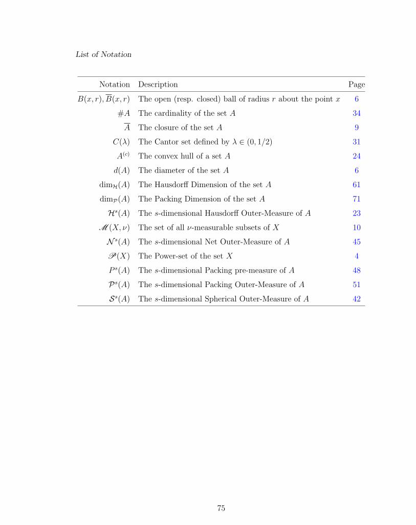
List of Notation

Notation Description Page

B(x, r), B(x, r) The open (resp. closed) ball of radius r about the point x 6

#A The cardinality of the set A 34

A The closure of the set A 9

C(λ) The Cantor set defined by λ ∈ (0, 1/2) 31

A(c) The convex hull of a set A 24

d(A) The diameter of the set A 6

dimH(A) The Hausdorff Dimension of the set A 61

dimP(A) The Packing Dimension of the set A 71

Hs(A) The s-dimensional Hausdorff Outer-Measure of A 23

M (X, ν) The set of all ν-measurable subsets of X 10

N s(A) The s-dimensional Net Outer-Measure of A 45

P(X) The Power-set of the set X 4

P s(A) The s-dimensional Packing pre-measure of A 48

Ps(A) The s-dimensional Packing Outer-Measure of A 51

Ss(A) The s-dimensional Spherical Outer-Measure of A 42

75

References

[HB01] Heinz Bauer, Measure and Integration Theory, de Gruyter Studies in Math-

ematics, vol. 26, Walter de Gruyter, Berlin, 2001. ↑10, 12

[ASB28] A. S. Besicovitch, On the fundamental geometrical properties of linearly

measurable plane sets of points, Mathematische Annalen 98 (1928), 422-

464. ↑43

[JMBFGST01] Jean-Marie Barbaroux, Francois Germinet, and Serguei Tcheremchantsev,

Generalized Fractal Dimensions: Equivalences and Basic Properties, Jour-

nal de Mathematiques Pures et Appliquees 80 (2001), 977-1012. ↑73

[GAE04] Gerald A. Edgar (ed.), Classics on Fractals, Westview Press, Oxford, UK,

2004. ↑1

[GAE91] , Measure, Topology, and Fractal Geometry, Springer-Verlag New

York Inc., New York, NY, 1991. ↑8, 10, 37, 71, 73

[GAE94] , Packing Measure as a Gauge Variation, Proc. Amer. Math. Soc.

122 (1994), 167-174. ↑56

[LCERFG92] Lawrence C. Evans and Ronald F. Gariepy, Measure Theory and Fine Prop-

erties of Functions, Studies in Advanced Mathematics, CRC Press, London,

UK, 1992. ↑41, 60

[HF69] Herbert Federer, Geometric Measure Theory, Springer-Verlag New York

Inc., New York, NY, 1969. ↑16, 20, 43

76

References

[KJF85] K. J. Falconer, The Geometry of Fractal Sets, Cambridge Tracts in Math-

ematics, vol. 85, Cambridge University Press, Cambridge, UK, 1985. ↑12,

25, 60, 63, 64, 68

[PH64] Paul Halmos, Measure Theory, D. Van Norstrand Company Inc., Princeton,

NJ, 1964. ↑9, 10, 12, 14, 25, 51

[HH86] Hermann Hasse, Non-σ-finite sets for packing measure, Mathematika 33

(1986), 129-136. ↑5, 52, 56, 72

[HJ99] H. Joyce, A Space on Which Diameter-Type Packing Measure is not Borel

Regular, Proceedings of the American Mathematical Society 127 (1999),

no. 4, 985-991. ↑57

[BM83] Benoit Mandelbrot, The Fractal Geometry of Nature, W. H. Freeman and

Company, New York, NY, 1983. ↑1, 3, 15

[PM95] Pertti Mattila, Geometry of Sets and Measures in Euclidean Spaces: Frac-

tals and rectifiability, Cambridge studies in advanced mathematics, vol. 44,

Cambridge University Press, Cambridge, UK, 1995. ↑25, 41, 43, 60, 71

[MM94] Mark McClure, Fractal Measures on Infinite Dimensional Sets (1994). ↑5,

47

[HLR68] H. L. Royden, Real Analysis, The Macmillan Company, New York, NY,

1968. ↑5, 10, 24, 35

[EMSRS03] Elias M. Stein and Rami Shakarchi, Fourier Analysis: An Introduction,

Princeton University Press, Princeton, NJ, 2003. ↑41

[SJTCT85] S. James Taylor and Claude Tricot, Packing Measure, and its Evaluation

for a Brownian Path, Transactions of the American Mathematical Society

288 (1985), no. 2, 679–699. ↑2

77

Documents

Construction of Geometric Outer-Measures and …loring/graduate_students/DaveWorth...Construction of Geometric Outer-Measures and Dimension Theory by David Worth B.S., Mathematics,