Embed Size (px)
Citation preview

1
CONSUMERS’ WILLINGNESS TO PAY FOR THE COLOR OF SALMON: A CHOICE EXPERIMENT WITH REAL ECONOMIC INCENTIVES
Frode Alfnes1, Atle Guttormsen1, Gro Steine2 and Kari Kolstad2
1Department of Economics and Resource Management Norwegian University of Life Sciences P.O. Box 5003, N 1432 Aas, Norway
Phone +47 6496 5700 Fax +47 6494 3012
E-mail: [email protected] E-mail: [email protected]
and
2Akvaforsk, Aas, Norway E-mail: [email protected]
E-mail: [email protected]
Selected Paper prepared for presentation at the American Agricultural Economics Association Annual Meeting, Providence, Rhode Island, July 24-27, 2005
Copyright 2005 by Frode Alfnes, Atle Guttormsen, Gro Steine and Kari Kolstad. All rights reserved. Readers may make verbatim copies of this document for non-commercial purposes by any means, provided that this copyright notice appears on all such copies.

2
CONSUMERS’ WILLINGNESS TO PAY FOR THE COLOR OF SALMON: A CHOICE EXPERIMENT WITH REAL ECONOMIC INCENTIVES
Abstract
We designed an experimental market with posted prices to investigate consumers’
willingness to pay for the color of salmon. Salmon fillets varying in color and price were
displayed in 20 choice scenarios. In each scenario, the participants chose which of two
salmon fillets they wanted to buy. To induce real economic incentives, each participant
drew one unique binding scenario; the participants then had to buy the salmon fillet they
had chosen in their binding scenario.
Key words: choice experiment, color, mixed logit, salmon, willingness to pay.
During the last decade, economists have used experimental markets to investigate
consumer preferences and willingness to pay (WTP) for food quality attributes. The most
popular method has been the second-price sealed-bid (Vickrey) auction where the
participants submit sealed bids for the product and the price is determined by the second-
highest bid (Vickery, Shogren et al., Alfnes and Rickertsen). The Vickrey auction is an
incentive compatible method for eliciting WTP; however, it is an unfamiliar market
mechanism for most consumers. Consumers are more familiar with markets where the
seller posts the prices and they, as consumers, have to choose which products to buy.

3
Lusk and Schroeder designed an experimental market with posted prices to
investigate consumers’ WTP for food quality attributes. They had five types of beef, and
ask the participants to choose which of the five types they would prefer to buy in 17
pricing scenarios. To induce real economic incentives, one of the price scenarios was
randomly drawn as binding. The participants had to buy the type of beef they had chosen
in the binding scenario and pay the respective price posted in that scenario. The choice
task in such an experiment is relatively close to the choice tasks consumers face in
grocery stores every day. Furthermore, it is in the participants’ own interest to choose the
alternative they prefer in each scenario, and their incentives to reveal true preferences is
relatively transparent. We will refer to such non-hypothetical choice experiment with
posted prices as real choice (RC) experiments.
We have conducted a RC experiment to investigate consumers’ WTP for salmon
with various degrees of flesh redness, and to investigate whether information on the
origin of the color influence consumers’ WTP. Salmon are recognized for their pink-red
flesh color, which distinguishes them from other species. Consumers use intrinsic cues
such as color to infer the quality of food products. In surveys as well as focus groups,
consumers have stated that they see the color of salmon as an indicator of flavor and
freshness, and it has been shown that redness contributes significantly to the overall
enjoyment of cooked salmon (Anderson, Sylvia et al.).
Consumers’ WTP for the color of farmed salmon is interesting for at least two
reasons. While wild salmon get their characteristic red color from the crustances they eat
in the sea. Farmed salmon get the color from synthetically produced feed additives.

4
However, the feed additive is expensive and the marginal return in form of color is
decreasing. Improved information on consumer WTP for salmon with various degree of
redness will help producers optimize the coloring. A second issue is the ongoing debate
of the “color added” label on farmed salmon. In recent years, consumer focus on food
safety, ethical production, and animal welfare has increased, and food additives used
partly or purely for cosmetic reasons are subject to considerable debate. The US Food
and Drug Administration require grocery stores to label farm-raised salmon so that
consumers are aware of the presence of artificial coloring. The fish should be labeled in
the retail case and on individual packages with the words “color added” or “artificially
colored”. In a survey of grocery stores in Iowa, we found that several stores still sold
farmed salmon that were not labeled with color added and we found none with color
added labeling on the retail cases. Furthermore, of the ones that did label the farmed
salmon, several used the less negative expression “the feeding process enhances the
color” instead of color added.
In 2003, consumer groups in the US filed a lawsuit against three major grocery
chains to force them to label the farm salmon as color added (Smith and Lowney). In a
class action complaint, it was stated: As a result of Defendant’s misbranding,
concealment and nondisclosure, consumers are misled to purchase the artificially
colored salmon and/or to pay a greater price than they would otherwise pay. Defendant
has been unjustly enriched at the expense of these consumers (Smith and Lowney).
Hence, Smith and Lowney argue that consumers’ WTP for farmed salmon would
decrease if they knew the origin of the color.

5
We use a modified version of Lusk and Schroeder’s RC design. Lusk and
Schroeder had the same five types of beef in all 17 price scenarios and used a fractional
factorial design to vary only the prices among the scenarios. They drew one binding
scenario for the whole group, so the choices where between types of beef and not
between specific packages. We used scenario specific products and used a fractional
factorial design to vary all product attributes among the scenarios. In each scenario, we
displayed two salmon fillets with varying colors and prices and the participants chose
which of the two salmon fillets they wanted to buy. To induce real economic incentives,
each participant drew one unique binding scenario. The participants then had to buy the
salmon fillet they had chosen in their binding scenario. The modified design is very
flexible and can easily be expanded to include a number of quality attributes.
To our knowledge, this is the first study using experimental markets to investigate
consumers’ WTP for seafood attributes. Only a few studies using various survey methods
has previously been conducted (Holland and Wessells, Johnston et al.; Wessells,
Johnston, and Donath). The remainder of the paper proceeds as follows: first, we give
some background information on farmed salmon, followed by a presentation of the
experimental procedure, products, design of choice scenarios, sample, and the
econometric model, the results and discussion, and last summary and conclusion.
Background
During the last few decades, the production of farmed salmon has experienced a growth
surpassed by few other primary production commodities. Global production increased

6
from about 12,000 metric tonnes in 1980 to well above 1 million metric tonnes in 2003.
However, such a large increase in production has significantly altered the structure of
several markets, and affected the pattern of international salmon trade. This has led to a
series of trade disputes, and the larges producers of farmed salmon, Norway and Chile,
have been subject to dumping complaints in both the US and the EU. See Anderson and
Fong, Asche, Bremnes and Wessels and Asche for discussions of some of the salmon
trade dispute cases.
The increase in production of salmon has been accompanied by a substantial
decline in prices. The main factors behind reduced production costs are improved
productivity and technological change. Fish farmers can today to a larger extent control
growth, sexual maternity, and quality parameters such as fat content, texture, taste, color
etc. However, while better control have reduced cost and improved the final product, the
industrialization of the salmon farming industry has at the same time lead to critical
voices among some researches, consumer groups and environmentalists (see for instance
Naylor et. al).
One of the issues of special concern among the above-mentioned group is the
salmon color. The characteristic color is caused by depositions of carotenoids in the
muscles. In the wild, salmon absorb carotenoids from the crustaceans they eat. The most
important carotenoid for the color of salmon is astaxanthin. Salmon are unable to
biosynthesize astaxanthin, and thus without astaxanthin in their diet, the salmons’ flesh
would range from gray or khaki to pale yellow or pale pink. Farm-raised salmon do not
have access to natural sources of astaxanthin. To impart the pink-red color in farmed

7
salmon, synthetically produced carotenoids, mainly astaxanthin, are added to their feed.
However, astaxanthin is expensive, and in conventional salmon farming astaxanthin
accounts for approximately 15 percent of the feed costs. Feed cost again accounts for
nearly 50 percent of total production costs (Guttormsen). Hence, coloring is a relatively
important cost in salmon farming. "In 2003, the total cost of producing 1 kilogram
slaughtered and gutted salmon in Norway was approximately NOK 20 and the cost of
producing one kilogram of salmon fillet was approximately NOK 34.1
The internationally recognized method for salmon color measurement is
comparing the salmon fillet flesh with the colors in the SalmoFanTM. The SalmoFan is a
color fan developed on the basis of the color of salmonid flesh pigmented with
astaxanthin. The color of conventional farmed salmon fillets sold in the Norwegian
market normally range from 23 to 30 on the SalmoFan, and most common are fillets
ranging from 25 to 27. In a consumer study conducted by Roche Vitamins, the producer
of astaxanthin for the salmon farming industry, they used the color 26 as their base
product (Fish Farming International).
Experimental Procedure
The experimental session included a survey2, a stated choice experiment, and an RC
experiment. The RC experiment consisted of three-times 10 choice scenarios.3 In each
choice scenario, the participants chose between two salmon fillets with posted prices. If
none of the alternatives was of interest, they could also select a none-of- these (NOT)

8
alternative. See table 1 for an example of the choice scheme. In this article, we will
analyze the first 20 RC scenarios that focused on the color of salmon.4
The RC experiment had nine steps. Step 1: The experimental procedure was
explained to the participants. Step 2: The participants studied the alternatives in scenarios
1 to 10, and marked on a choice scheme which of the alternatives in each scenario they
wanted to buy. Step 3: The participants were informed about the origin of the color. Step
4: The participants studied the alternatives in scenarios 11 to 20, and (as in Step 2)
marked on a choice scheme which of the alternatives in each scenario they wanted to buy.
Step 5: The participants were informed about organic and ecolabeled salmon. Step 6: The
participants studied the alternatives in scenarios 21 to 30, and (as in Steps 2 and 4)
marked on a choice scheme which of the alternatives in each scenario they wanted to buy.
Step 7: After all participants had completed all scenarios, each participant drew one card
determining his or her binding scenario. The drawing was done without replacement, so
that only one participant was assigned to each scenario. Step 8: Each participant got the
salmon fillet he or she had chosen in his or her binding scenario. Step 9: The participants
went to the cashier and paid for their salmon fillets.
The design of our experiment follows Lusk and Schroeder with some important
modifications. First, we used scenario-specific products. We had 30 boxes filled with ice
on three large tables. Each of the boxes represented one scenario. In each box we
displayed two consumer packages of salmon fillets. The prices of the two alternatives
were posted on laminated paper in the back of the box. This setup is very flexible and
allowed us to vary not only the price but also the products among the scenarios. Second,

9
the participants chose between the exact product packages they could obtain. Each
participant randomly drew his or her exclusive scenario, and the participant that drew
scenario four would obtain the fillet he or she had chosen in box number four. The
salmon fillets they evaluated were the exact same fillets they would buy. For this to be
possible, the number of participants in each session had to be smaller or equal to the
number of choice scenarios. Third, the two alternatives in each box were referred to as
Alternative 1 and Alternative 2. The only information that was posted in our experiment
was the price. The consumers had to infer the quality from intrinsic quality cues such as
color. Extending the design to include other types of information such as labeling is
straightforward. Fourth, the color, as well as the price, was a part of the fractional
factorial design, as was the positioning of the products as Alternative 1 or Alternative 2.
Any left or right hand side bias would therefore have no effect on the relative utility of
the alternatives. Fifth, before the first 10 scenarios we did not give the participants any
information about how the salmon fillets differed. We said that we had various types of
farmed salmon fillets, and asked the participants to study the alternatives and choose the
alternative they would like to buy, given the price. Only after the first 10 scenarios, we
informed the participants about the origin of the color. Sixth, to reduce any systematic
ordering effects the participants could start at any of the 10 scenarios on each table. This
also speeded up the process and we avoided a queue in front of the first scenario.
Our modification of the design was inspired by the growing literature on stated
choice (SC) surveys. Lusk and Schroeder include all alternatives in every scenario, and
varied only the prices among the scenarios. This limits the number of alternatives that can

10
be included in the experiment. In the SC literature, consumers choose among alternative
product descriptions in hypothetical scenarios. In SC surveys it is common to include a
large number of quality attributes, both existing and nonexisting. To elicit consumer
preferences for the attributes efficiently, fractional factorial design is used to vary all
attributes among the scenarios. To lessen the cognitive burden on the participants, usually
only two or three alternatives are included in each scenario. For a thorough survey of SC
methodology and applications, see Louviere, Hensher and Swait.
As a result of the modification of the design, fewer products are needed. In a
choice experiment where all products are available in each choice scenario, it is possible
that all participants end up with the same product. Assuming that we have n alternatives
and m participants, we would then need m products of each of the n alternatives, m*n
products. Including only two alternatives in each choice scenario and allowing each
participant to draw his or her exclusive scenario, reduces the total number of products
necessary to 2*m, or 2*m/n products of each alternative.
Products
To ensure a large variation in color, we bought salmon from four different production
sites: three conventional salmon farms that utilize synthetically produced astaxanthin and
one organic salmon farm that only uses astaxanthin from natural sources. The salmon
fillets were cut into portions weighing approximately 400 grams5, put into packaging
familiar to consumers, exactly weighted, and we recorded if the fillet portions were from
the front or tail of the fillet. The fillets were categorized into color categories using the

11
internationally recognized method for color measurement for salmon, the SalmoFanTM.
Fillets from the conventional salmon farms ranged in color from 23 to 30 on the
SalmoFan, and those from the organic salmon farm ranged from 20 to 22. The fillets
were grouped into five color categories, hereafter referred to as alternatives R21, R23,
R25, R27, and R29.
The price attribute took the levels NOK 24, 30, 36, 42, and 48. This corresponds
to a price per kilogram of NOK 60, 75, 90, 105, and 120, respectively. The week before
the experiment, the prices of salmon fillets in the three largest grocery stores in the area
were NOK 79, 89, and 119 per kilogram. Thus, all prices except for that of NOK 24 were
within a familiar price range for salmon fillets in Norway.
Non-processed food products such as salmon fillets are heterogeneous in so many
ways that we cannot obtain products that are uniform in all characteristics. Allowing the
color categories to be represented by more than one product gives a better representation
of the categories than selecting one product from each category. In our experiment, we
had eight sessions, 20 color scenarios with two fillets in each scenario. Each color
category was included eight times in each session. We replaced the fillets every day, and
the fillets sold in the first session each night were replaced with new fillets. The total
number of fillets displayed in the color experiment was 197, divided into five color
categories. On average, each color category was represented by almost 40 salmon fillets
in the experiment. This relative high number of salmon fillets in each color category
reduce the effect on the WTP estimates of any unrecorded attributes of one specific
salmon fillet.

12
Design Choice Scenarios
We used a SAS macro to generate a fractional factorial design with 40 choice scenarios.
Each scenario had two alternatives described by color and price, both five-level
attributes. To avoid clearly dominated alternatives we limited the design to scenarios
where the color of the two alternatives differed. There were, however, no limitations on
the price attribute, and several scenarios had the same price for both alternatives. The
scenarios were divided into four blocks, and randomly arranged within the blocks. SAS
reported a D-efficiency of 96.85 for the design. Each block of scenarios was used once as
scenario 1 to 10, and in another session as scenario 11 to 20. For a description of the SAS
macro, see Kuhfeld.
Sample
The experiment was conducted at MATFORSK, The Norwegian Food Research Institute,
during four nights in February 2004. We conducted two sessions each night, and the
sessions lasted approximately one and a half hours each. Each session had between 13
and 16 participants. In total, 115 participants were recruited through various local
organizations, including choirs and soccer teams, in southeastern Norway. In each
organization, the contact person was instructed to provide a sample of regular consumers,
between 25 and 60 years old, with an approximately equal division of sexes. The
organizations were given NOK 200 for each participant they recruited, and the
participants were given NOK 300 to take part in the experiment.
13
Table 3 presents the descriptive statistics for the sample. The participants’ ages
ranged from 20 to 63 years, with an average of 39 years. Fifty eight percent of the
participants were women. The average household income was NOK 562,000. One
participants that said he did not eat fish, and 15 participants that chose the NOT
alternative in all choice scenarios were excluded from the analysis. The sample used in
the estimation consists of the remaining 99 respondents.6
Econometric Model
We analyzed the RC data with a mixed logit (also known as a random parameter logit)
model. The mixed logit obviates three of the limitations of the standard logit model by
allowing for random taste variation, unrestricted substitution patterns, and correlation in
unobserved factors over time (Train). Furthermore, McFadden and Train show that under
mild regularity conditions, any discrete choice model derived from random utility
maximization has choice probabilities that can be approximated as closely as one pleases
by a mixed logit model.
Let us assume that the individual’s utility from each alternative can be
decomposed into a linear-in-parameters part that depends on observable variables, and an
error term that is independently and identically distributed (iid) extreme value. Given
these assumptions, the utility of individual n from alternative i in choice scenario s is
denoted by:
(1) nis nis n nis nisU = x + z′ ′β η + ε

14
where xnis and nisz are vectors of observed variables relating to alternative i; β is a vector
of fixed coefficients;η is a vector of random terms with mean zero; and nis is an iid
extreme value error term. The terms inη are error components that, along with nis, define
the stochastic portion of the utility. The standard logit is a special case of the mixed logit
whereη has zero variance.
The density of η is denoted by f(η|Ω) where Ω is the fixed parameters of the
distribution. For a given η, the conditional choice probability is a standard logit:
(2) e
)e
ni n ni
nj n nj
x + z
ni x + z
j J
L ( β η
β η
′ ′
′ ′
∈
=
Consequently, the unconditional choice probability, P, in the mixed logit model is the
logit formula integrated over all values of η with the density of η as weights:
(3) ni niP = L ()f( |)d
This choice probability cannot be calculated exactly and is approximated through
simulation (Brownstone and Train).
In the RC color experiment, the participants were asked to make 20 choices
between salmon fillets offered at various prices. The choice data were analyzed with the
following mixed logit model:
(4) 0 1 2 3 4( ) 24nis i nis i s ni nis nis nis nisU Tail ID Weight Price Priceβ β β η β β ε= + + + + + +

15
where 0iβ is the alternative specific constant for alternative i, ASC(i) (in other words,
there is one constant for each color); nisTail is a dummy taking the value one if the
product is a fillet tail, and zero otherwise; IDs is a dummy variable taking the value zero
before the color information was given and one afterwards; niη is a error term that is
triangularly distributed, heteroscedastic, independent between alternatives, and perfectly
correlated over choices made by the same individual7; Weightnis is the exact weight of the
alternative i in kilograms; Pricenis is the price of alternative i; Price24nis is a dummy
taking the value one if the price is NOK 24, and zero otherwise. The Price24-dummy is
included to capture any adverse effects of offering the salmon fillets at price that is below
what is normally seen in the market. For identification, the alternative-specific
parameters for the palest alternative, R21, is normalized to zero. For the estimation
purposes, the weight of the NOT alternative is set to one.
The mean WTP per kilogram of alternative i can be calculated by dividing the
utility difference between the one kilogram of the varieties and the NOT alternative, with
the negative of the price sensitivity parameter:
(5) 0 1 2 0 2
3
( ) ( )100* i is i s NOT NOT s
is
Tail ID IDWTP
β β β β ββ
+ + − += −
where WTPis is the estimated mean WTP per kilogram of alternative i in scenario s; and
all other variables and parameters are as described in equation (4). Since the price
sensitivity parameter measures the utility of the price in NOK 100, we must multiply the
result by 100 to get the WTP in NOK:

16
Results and Discussion
In our design, there were no correlation between color and price and no correlation
between the price of alternative 1 and the price of alterantive2. Therefore, one would
expect that on average the choice probability for an alternative increased as the price
decreased. This was the case as long as the price was within the familiar price range of
NOK 30 to NOK 48 per 400 grams. However, when the price was reduced from NOK 30
to NOK 24 the average choice probability for an alternative was reduced. On average, the
percentages of the participants that chose an alternative with a price of NOK 48 was
30.76%, this increased to 35.98% for NOK 42, 37.71% for NOK 36 and 42.86% for
NOK 30, but decreased to 36.78% for NOK 24. The NOK 24 price is below that which is
normally seen in the market, and it appears that this low price is seen as a signal of low
quality. Not controlling for this would give a price sensitivity parameter that was closer
to zero, and thereby higher WTP values.
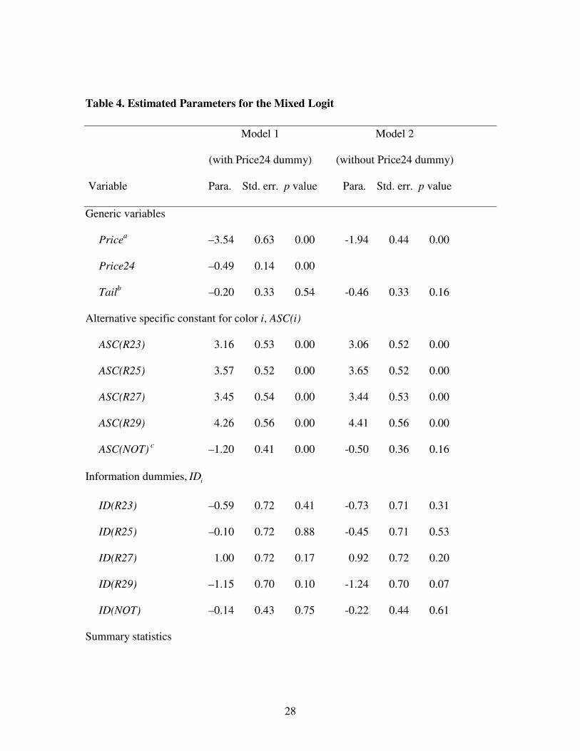
Table 4 shows the estimated parameters, standard errors, and p-values for the
mixed logit model with and without the Price24 dummy. The Price and NOT parameter
change considerably when we exclude the Price24 dummy. The Price parameter change
because the adverse reaction to the NOK 24 price is not accounted for with a dummy, but
instead is interpreted as a lack of price sensitivity. Furthermore, with a reduced absolute
value on the Price parameter, the NOT parameter must increase to compensate for the
loss in the NOT alternatives’ relative utility resulting from its zero price.

17
We will from now on, concentrate the discussion on model 1. From the lower part
of table 4, we can see that the mixed logit model (log likelihood of -1808) fits the data
significantly better than the more restrictive standard logit model (log likelihood = -
2051).
The ASC represents the utility per kilogram of the alternatives before we
informed the participants about the origin of the color. It is worth noting that these color
preferences were elicited without telling the participants that they should focus on color.
The ASC for the colors R23, R25, R27, and R29 are all positive and significant. This
means that on average the consumers preferred these colors to the paler R21.
Furthermore, the alternative with the highest utility is the reddest alternative, R29. The
ASC of R29 is significantly higher than the ASC of the paler R23 (Wald, p value = 0.00),
and R27 (Wald, p value = 0.02), and higher, but not significantly, than R25 (Wald, p
value = 0.07), No significant differences were found between the alternatives R23, R25,
and R27.
The ASC plus the ID represent the utility per kilogram of the alternatives after we
informed the participants about the origin of the color. None of the utilities changed
significantly after the color information was presented. The utilities of the colors R23,
R25, R27, and R29 are still positive and significant. This means that the average
consumer prefers the redder colors to the pale R21 even when they know the origin of the
color. However, the utility of the reddest alternative, R29, decreased significantly relative
to the utility of R25 (Wald, p value = 0.05) and R27 (Wald, p value = 0.00), and decrease,
but significantly, relative to the utility of R23 (Wald, p value = 0.26). After the color

18
information was supplied, the utility of R27 is significantly higher than the utility of R23
(Wald, p value = 0.00), R25 (Wald, p value = 0.01), and R29 (Wald, p value = 0.01).
The number of fillet tails was unevenly distributed among the five color
categories and was most frequent in the R29 category. The tail parameter was not found
to be significant, although the negative value indicate that the participants preferred the
thicker front part of the fillet to the tail of the fillet.
Table 5 presents the WTP per kilogram of the five alternatives. As discussed
above, the participants preferred the reddest alternative, R29, when they were
uninformed, and the slightly paler R27 when they were informed about the origin of the
color. After the information the participants still preferred fairly red salmon, but they
seemed to have become a little skeptical with respect to salmon that were redder than
they were used to. This is reflected in figure 1 where the concave nature of the WTP for
color is evident.
Remembering that the price of salmon fillets in the local stores ranged from NOK
79 to NOK 119 the week before the experiment, we find the level of the WTP estimates
surprisingly high. The high WTP estimates indicates that the participants did not take
their outside options fully into account, and thereby chose one of the salmon alternatives
to often. A higher percentage of NOT choices would have increased the estimated utility
parameter for the NOT alternative, and through equation (5) reduced the level of all
salmon WTP estimates. It is important to understand, that including the 15 participants
that chose the NOT alternative in all 20 scenarios would not help much. We have used a
panel version of the mixed logit model, were all choice made by one participant are

19
clustered together. Including 15 participants that make the same choice in all 20 scenarios
would have little effect on the parameter included in equation (5), however it would
significantly increase the variance of the non-iid error term associated with the NOT
alternative.
An alternative explanation of the high WTP estimates is that the price sensitivity
parameter that comes from the marginal changes in the product attributes, are less than
the price sensitivity for the product as a whole. In other words, that the price sensitivity
we find is a marginal price sensitivity that should not be used to draw conclusions about
the total WTP. We the data we have from this experiment, we cannot distinguish between
this two explanations. Further research is necessary before we fully understand how
outside options and other framing effects influence consumers’ decisions in choice
experiments.
Summary and Conclusion
In RC experiments, consumers face choices involving real products and money in a series
of choice scenarios. The choice task is relatively similar to the choices consumers face in
grocery stores. The incentives for revealing one’s true preferences are transparent. This
makes the RC experiments an incentive compatible method for eliciting WTP for food-
quality attributes. The design of the experiments and the analysis of the data are based on
methods developed for hypothetical choice experiments. We modify the RC design by
using scenario-specific products and unique binding scenario for each participant. This
increases the flexibility, allows for incorporation of a higher number of quality attributes,
20
and allows the participants to choose between specific product packages and not only
product types.
The RC experiment presented in this article focuses on the color of salmon. The
pink-red color is one of the most important quality traits for Atlantic salmon. Consumers
use the color as a quality indicator and are willing to pay significantly more for salmon
fillets with normal, or above normal redness, compared with paler salmon fillets. Without
artificial coloring, farm-raised salmon would be difficult to market, and would command
lower prices. Salmon with a color below 23 on the Roche Salmofan is difficult to sell at
any price. However, there is less to gain by increasing the color above 23. Informing the
consumers about the origin of the color does not affect the WTP for pale and normal red
fillets. However, this information does influence the WTP for above normal red fillets,
which decreases significantly. These results indicate that color-added labeling would
have little effect on the demand for the most common color categories of farmed salmon.
Consumer WTP for various degrees of redness is only a part of the information
necessary to find the optimal level of coloring for salmon. In addition, estimates of the
cost of increasing the color and information about to what extend the producers are able
to retrieve the increasing WTP are necessary to solve the optimization problem. Further
research should be conducted in these areas.

21
Footnotes
1NOK 100 = EUR 11.44 = US$ 14.34. February 4, 2004. (www.oanda.com).
2 The survey was divided into four parts. The participants answered most questions
before the choice experiment, some questions after 10 choice scenarios, others after 20
choice scenarios, and the last questions after all 30 choice scenarios had been completed.
In this article, we will not utilize the survey response.
3 The instructions are available from the authors upon request.
4 The last 10 scenarios, focusing on organic and ecolabeled salmon, will be analyzed in
another article.
5 The mean weight was 400.28 gram with a standard deviation of 40.25 gram. To avoid
that the weight played an important role in the choice, we had a 10% upper limited of
how much a choice pair were allowed to differ.
6 Norway has a high organizational participation rate. In the Oslo area, for example, 49%
of the population responds that they actively participate in at least one organization
(Statistics Norway). Recruiting through organizations, therefore, can give a representative
sample of the population.
7 See Hensher and Greene for a discussion of various distributions on the non-iid error
term.

22
References
Alfnes, F., and K. Rickertsen. “European Consumers’ Willingness to Pay for U.S. Beef in
Experimental Auction Markets.” American Journal of Agricultural Economics
85(2003):396–405.
Anderson, S. “Salmon Color and the Consumer.” In Proceedings of the IIFET 2000
International Institute of Fisheries Economics and Trade. Corvallis, OR: Oregon
State University, July 10–14, 2000.
Anderson, J.L. and Q.S.W. Fong. “Aquaculture and International Trade.” Aquaculture
Economics and Management 1(1997):29–44.
Asche, F. “Testing the Effect of an Anti-dumping Duty: The US Salmon Market.”
Empirical Economics 26(2001):343–55.
Asche, F., Bremnes, H., and C.R. Wessells. “Product Aggregation, Market Integration
and Relationships Between Prices: An Application to World Salmon Markets.”
American Journal of Agricultural Economics 81(1999): 568-81.
Brownstone, D., and K. Train. “Forecasting New Product Penetration with Flexible
Substitution Patterns.” Journal of Econometrics 89(1999): 109–29.
Fish Farming International. “Consumers ‘Will Pay More for Darker Salmon’: Study.”
30(2003:2):35.
Guttormsen, A.G. “Input Factor Substitutability in Salmon Aquaculture.” Marine
Resource Economics 2(2002): 91–102.
Hensher, D.A., and W.H. Greene. “The Mixed Logit Model: The State of Practice.”
Transportation 30(2003): 133–76.

23
Holland, D., and C.R. Wessells. “Predicting Consumer Preferences for Fresh Salmon:
The Influence of Safety Inspection and Production Method Attributes.”
Agricultural and Resource Economics Review 27(1998): 1–14.
Johnston, R.J., C.R. Wessells, H. Donath, and F. Asche. “Measuring Consumer
Preferences for Ecolabeled Seafood: An International Comparison.” Journal of
Agricultural and Resource Economics 26(2001):20–39.
Kuhfeld, W.F. Standard Logit, Discrete Choice Modeling: An Introduction to Designing
Choice Experiments, and Collecting, Processing, and Analyzing Choice Data with
SAS. TS-643. Cary, NC: SAS Institute Inc., 2001.
Lusk, J.L., and T.C. Schroeder. “Are Choice Experiments Incentive Compatible? A Test
with Quality Differentiated Beef Steaks.” American Journal of Agricultural
Economics 86(2004): 467–82.
Louviere, J.J., D.A. Hensher, and J.D. Swait. Stated Choice Methods: Analysis and
Application. Cambridge: Cambridge University Press, 2000.
McFadden, D., and K. Train. “Mixed MNL Models for Discrete Response.” Journal of
Applied Econometrics 15(2000): 447–70.
Naylor, R.L., R.J. Goldburg, J.H. Primavera, N. Kautsky, M.C.M. Beveridge, J. Clay, C.
Folke, J. Lubchenco, H. Mooney, and M. Troell. “Effect of Aquaculture on World
Fish Supplies.” Nature 405(2000):1017–24.
Shogren, J.F., S.Y. Shin, D.J. Hayes, and J.B. Kliebenstein. “Resolving Differences in
Willingness to Pay and Willingness to Accept.” American Economic Review
84(1994): 255–70.

24
Smith and Lowney, P.L.L.C. Nationwide Class Actions Target Major Grocery Store
Chains for Concealing Artificial Coloring in Farm-Raised Salmon. 2003.
<http://www.smithandlowney.com/salmon> (March 13, 2004).
Sylvia, G., M.T. Morrissey, T. Graham, and S. Garcia. “Organoleptic Qualities of Farmed
and Wild Salmon.” Journal of Aquatic Food Product Technology 4(1995): 51–64.
Train, K. Discrete Choice Methods with Simulation. Cambridge: Cambridge University
Press, 2003.
Vickery, W. “Counterspeculation, Auctions, and Competitive Sealed Bids.” Journal of
Finance 16(1961):8–37.
Wessells, C.R., R.J. Johnston, and H. Donath. “Assessing Consumers Preferences for
Ecolabeled Seafood: The Influence of Species, Certifier, and Household
Attributes.” American Journal of Agricultural Economics 81(1999):1084–9.

25
Table 1. Example of Choice Scheme
400 grams farmed salmon Scenario
1 Alternative 1 Alternative 2 None of these
NOK 36 NOK 48
I would choose (check one)

26
Table 2. Information Given to the Participants
The fillets from wild salmon are usually pink, red, or orange. The strength of the color
can vary from salmon to salmon. The color originates from carotenoids in the fish’s diet.
Carotenoids are widespread in living organisms.
The most important carotenoid for the color of salmon is astaxanthin. Astaxanthin is a
common substance in both fresh water and marine organisms. Wild salmon get
carotenoids from eating crustaceans, or small fish that themselves have recently eaten
such animals.
To create similar color in farmed salmon, synthetically produced astaxanthin is added
to their feed. No negative side effects have been reported from the use of astaxanthin.

27
Table 3. Descriptive Statistics for the Sample
Variable Definition Meana St.dev.
Gender Gender of participant 1.43 0.49
Female = 1; Male = 2
Age Age of participant 38.81 10.29
Income Total income of householdb 5.62 2.63
(in NOK 100 000)
Education Highest completed education 2.54 0.67
Elementary school = 1
High school = 2
College/University = 3
aCorresponding figures for the population between 20 and 60 years old in the Oslo area
are 1.49, 39.80, 5.89, and 2.41, respectively.
bThe income question had six classes. The midpoints of classes are used in the estimation.
28
Table 4. Estimated Parameters for the Mixed Logit
Model 1 Model 2
(with Price24 dummy) (without Price24 dummy)
Variable Para. Std. err. p value Para. Std. err. p value
Generic variables
Pricea –3.54 0.63 0.00 -1.94 0.44 0.00
Price24 –0.49 0.14 0.00
Tailb –0.20 0.33 0.54 -0.46 0.33 0.16
Alternative specific constant for color i, ASC(i)
ASC(R23) 3.16 0.53 0.00 3.06 0.52 0.00
ASC(R25) 3.57 0.52 0.00 3.65 0.52 0.00
ASC(R27) 3.45 0.54 0.00 3.44 0.53 0.00
ASC(R29) 4.26 0.56 0.00 4.41 0.56 0.00
ASC(NOT) c –1.20 0.41 0.00 -0.50 0.36 0.16
Information dummies, iID
ID(R23) –0.59 0.72 0.41 -0.73 0.71 0.31
ID(R25) –0.10 0.72 0.88 -0.45 0.71 0.53
ID(R27) 1.00 0.72 0.17 0.92 0.72 0.20
ID(R29) –1.15 0.70 0.10 -1.24 0.70 0.07
ID(NOT) –0.14 0.43 0.75 -0.22 0.44 0.61
Summary statistics

29
Number of observations 1977 1977
Number of participants 99 99
LL standard logit –2051 -2058
LL mixed logit –1808 -1814
Notes: Estimated with Nlogit 3.0.
aPrice in NOK 100.
bTail is one if tail, zero otherwise. The variable is centralized before the estimation.
cNOT stands for Neither Of These.

30
Table 5. Willingness to Pay per Kilogram of Salmon
Before information After information
Color WTP Std. err WTP Std. err
R21 36.51 9.21 38.00 8.80
R23 126.10 19.70 110.87 17.37
R25 137.62 21.87 135.68 20.01
R27 133.96 21.35 163.23 25.05
R29 156.92 25.31 125.99 20.69

31
0.00
50.00
100.00
150.00
200.00
R21 R23 R25 R27 R29
Color
NO
K
Before information After information
Figure 1. Willingness to pay per kilogram of salmon before and after information