Embed Size (px)
Citation preview
Container transshipment and port competition
*Bae Minju, *Ek Peng Chew, *Loo Hay Lee, +Anming Zhang
*Department of industrial and Systems Engineering
National University of Singapore
+Sauder School of Business
University of British Columbia
November 2011
Abstract
This study investigates duopolistic competition between hub ports for container
transshipment. A container handling demand function which incorporates both gateway and
transshipment traffic is developed. The study applies a non-cooperative two-stage game to a
vertical-structure seaport market with ports as upstream players and shipping lines as
downstream players. We explain the drivers behind port competition through the existence of
a unique Nash equilibrium which incorporates the shipping lines’ supply decision and the
ports’ pricing decision. We also analyze a port collusion model and a social optimum model,
and compare it with the non-cooperative model for further insights.
Keywords: Container transshipment, Port competition, Non-cooperative game, Two-stage
game, Nash equilibrium
1. Introduction
In 2000, Maersk Sealand relocated its major transshipment operations from the Port of
Singapore (PSA) to the Port of Tanjung Pelepas (PTP) in Malaysia. The impact of this
relocation on the regional transshipment market structure was significant. Maersk Sealand
was then the largest shipping operator in Singapore. Its shift to PTP resulted in a decline of
approximately 11% in PSA’s overall business. In 2001, PSA’s total container throughput fell
from 17 million TEUs to 15.52 million TEUs, marking a year-on-year drop of 8.9%
(Tongzon, 2006). In the same period, PTP’s container throughput had increased nearly 5
folds, from 0.42 million to 2.05 million TEUs.1
The shipping industry in Singapore and the region grew concerned about Maersk
Sealand’s relocation and the potential ripple effect on other shipping lines’ decisions and
related business activities.2 As shipping lines form strategic alliances to achieve economies of
scale, the interdependency among alliance members and small- and medium-size shipping
lines heightens. Consequently, Maersk Sealand’s decision on changing its transshipment port-
of-call could well induce similar decisions among affiliating carriers. In 2002, Evergreen and
its subsidiary Uniglory followed in Maersk Sealand’s footsteps and shifted most of their
container operations, amounting to 1-1.2 million TEUs of annual throughput, from PSA to
PTP. Since then, other shipping lines have also started to provide direct services to PTP.
APL, for example, had chosen PTP for its West Asia Express service between Asia and the
Middle East (Kleywegt et al., 2002).
This study aims to investigate a regional transshipment hub port competition problem
within a duopolistic framework. In the case of competition between PTP and PSA, the
acquisition of transshipment cargo is critical. Both ports are subjected to stringent growth
limitations as gateway ports but possess excellent locations along the Strait of Malacca.
Transshipment presents a good opportunity for these ports to expand beyond the demands of
their respective catchment economies and more importantly, tap into the international cargo
flows to enjoy superior profits. Beyond the potential spike in the number of cargo handling
jobs and value-added activities, a transshipment port would also gain access to profitable
feeder line networks which serve to transport containers to/from tributary ports. These
networks give the transshipment port good connectivity, which in turn strengthens itself
through the “ripple effect”. As the importance of achieving dominance in the market becomes
apparent, it is foreseeable for regional ports to compete for transshipment container traffic.
In particular, we construct a demand function for a container port’s transshipment traffic.
A review of the existing studies of port selection and competition (Lirn et al., 2003, 2004;
Chou, 2007; Lin and Tseng, 2007; Chang et al., 2008; Yuen et al., 2011) have led us to
1 The container throughput data is taken from the official website of Port of Tanjung Pelepas, http://www.ptp.com.my/history-2000.html and http://www.ptp.com.my/history-2001.html. 2 The issue was, for example, discussed in the article written by Allison of Asia Times Online on 2 September 2000.
identify port capacity, price, “transshipment coefficient” and port congestion as the primary
factors of relevance to our study. While the port price and transshipment coefficient primarily
determine the demand levels of a port,3 the resulting level of demand, together with the port
capacity, determine the port’s congestion level, which in turn will influence the demands of
the port and its rival port. This study attempts to uncover the relationships with greater
clarity. In particular, we examine how different levels of port capacities, prices and
transshipment coefficients affect the ports’ congestion levels and, more importantly, how a
port can capture a greater transshipment demand with appropriate port pricing and capacity
building.
We find that (i) at the non-cooperative model, the price difference between two ports is
further accentuated when both port capacities are large, as in this case, congestion becomes
less of an inhibiting factor. (ii) Shipping lines are inclined to make more port calls at the port
that provides a higher transshipment coefficient, as long as the port capacity is sufficient to
offset the accompanying congestion delay cost. (iii) The ports do take into consideration their
capacity when setting prices. A bigger port can set a lower port price to attract more demand
as it is more likely to have spare capacity and hence less congestion. (iv) The port collusion
model yields a higher port price than that of non-cooperative model. (v) The profit margin of
the social optimum model is higher than that of the non-cooperative model. The port price is
internalized in the social optimum model therefore shipping lines can make more port calls
than that of the non-cooperative model.
A number of studies have looked at port competition: Lam and Yap (2006, 2007)
examined port competitiveness and the impact of competition in Southeast Asia while Yap
and Lam (2006) considered the case of East Asia and Anderson, et al. (2008) considered the
case of Northeast Asia. Saeed and Larsen (2010) considered intra-port competition and
examined the possible combinations of coalitions among container terminals at the Karachi
Port of Pakistan. Port competition is further investigated as part of rivalry between two
alternative intermodal transportation chains; hence, recent studies have taken into account
hinterland access and road congestion in order to observe their impact on ports and port 3 As global customers exert increasing pressure on shipping lines to lower their prices, the competition to reduce costs among shipping lines inevitably intensifies. Shipping lines are forced to explore the cheapest-cost options which in turn impose downward pressure on the port charges. For instance, the attractiveness of PTP’s port price, which is some 30% lower than that of PSA’s, becomes apparent. In fact, Evergreen had estimated that its shift to PTP would result in cost saving of between US$ 5.7 million and US$ 30 million per annum (Kleywegt et al., 2002). As such, port price will affect port demand. As for “transhipment coefficient,” it measures port connectivity and efficiency (the transhipment-coefficient definition is given below in section 2), which will affect the decision of shipping lines’ choice of port, thereby affecting port demand.
competition (Zhang, 2008; Yuen, et al., 2008; Wan and Zhang, 2011; Wan et al., 2011).
Unlike our consideration of “transshipment container demand,” these papers have focused on
“gateway container demand” – these are two different types of container demand at a
transshipment port. The gateway demand represents the import and export container
demands, whilst the transshipment demand is generated through the additional container
handling jobs necessary for further seaborne transfers after unloading, including
consolidation, deconsolidation and value-added activities of containers.4 Our transhipment
focus can help advance the analysis on a port’s transshipment capabilities and enable the port
to uncover and balance its demand and capacity levels so as to strategize for the long term. It
can also provide better visibility on the shipping lines’ criteria when choosing a
transshipment port.
Our study is closely related to the applications of game theory to port competition
problem. Zan (1999) was one of the earliest authors who had attempted to use the game
theory to investigate the behaviour of port users (carriers and shippers) in transshipment port
management policy. He used a bi-level Stackelberg game to capture the flow of foreign trade
containers. In more recent studies, Saeed and Larsen (2010) used the two-stage game to
analyze possible coalitions: in the first stage, three container terminals at Karachi Port decide
whether to act individually or to join a coalition; and in the second stage, the resulting
coalition plays a non-cooperative game against non-members. In another study relevant to
our work, De Borger, et al. (2008) used a two-stage game to analyze the interaction between
the pricing behaviour of competing ports and the optimal investment policies in the ports and
hinterland capacity. Beyond maritime-related research, studies have been performed on the
duopolistic interactions between congestible facilities using a two-stage game (e.g. Van
Dender, 2005; De Borger and Van Dender, 2006; Zhang and Zhang, 2006; Baake and
Mitusch, 2007; Basso and Zhang, 2007).5 For example, Basso and Zhang (2007) developed a
model for congestible facility rivalry in vertical structures which explains the relationship
among the congestible facility and its intermediate user (airline) and final users (passengers).
We will leverage on this approach to explain the drivers behind the container transshipment 4 The import container demand is further defined as containers destined for hinterland transportation out of the port after unloading from the vessels, and the export container demand as containers meant for seaborne transfer out of the port. The distinction between gateway and transhipment demands has been discussed in air transport research by Zhang (2003), where “gateway” traffic refers to “local and gateway” traffic, whereas “transshipment” traffic to “hub” (air to air) traffic. 5 As defined by De Borger and Van Dender (2006), congestible facilities are facilities which are prone to congestion when the volume of simultaneous users increases amid constant capacity. Examples of such facilities include seaports, airports, Internet access providers and roads.
port competition through the existence of a unique Nash equilibrium for the shipping lines’
supply and the port pricing. We will also analyze a port collusion model and a social
optimum model, and compare it with the non-cooperative model for further insights, where
the port collusion model can behave like a monopoly, whereas the social optimum model
reflects a maximization of the combined profits of all the players in the game.
The paper is organized as follows: Section 2 shows our model formulation with linear
container handling demand functions. We then proceed to apply the non-cooperative two-
stage game to our problem in section 3. In section 4, a port collusion model, and a social
optimum model which may reflect the current business models of shipping lines, are analyzed
and compared with the non-cooperative model. Results from our numerical simulations are
then shown in section 5 to further explain the findings of this study. Finally, section 6
contains the concluding remarks.
2. The model
We assume there are two container transshipment ports, r =1, 2, which provide homogenous
container handling services to their customers within a stipulated period of time. Their
customers are identical shipping lines, i=1,…, N.
The notations used for developing our model are defined as follows;
loaded and unloaded gateway container demand
coefficient of loaded and unloaded transshipment container volume
number of ocean carriers
a fraction of transshipment port calls made by carrier
r
ir
f
g
N
q at port
price per container charged by carrier
carrier 's operating cost per container
total loaded and unloaded containers of carrier at port
profit for carrier
port pri
i
i
ir
i
r
i r
p i
c i
F i r
i ce per container at port
85% capacity utilization of port
profit for port r
r
r
K r
r
1
1
total fraction of transshipment port calls at port
total container demand at port
( , ) cost of congestion delays per container at port
N
r iri
N
r iri
r r r
Q q r
F F r
D F K r
Our container handling demand function, irF , is the total number of containers which carrier
i loads and unloads at port r.
for 1,2 (1)ir r rF f g Q r
where 1
N
r iriQ q
, 0 1irq , 1 for is irq q r s and gr is nonnegative coefficient. qir
is a decision variable which indicates a fraction of transshipment port calls that carrier i
makes at port r, and is determined by the capacity of port r, its price and transshipment
coefficient during the stipulated period of time.
Fir is made up of two components: The gateway container, i.e. import and export container
demand, and the transshipment container that is generated through transshipment
performance at port r. f is the gateway container demand that the shipping line handles at
port r, which is inclusive of both the unloading of import containers and loading of export
containers. Since this study focuses more on the impact of transshipment demand, we assume
that the gateway container demand is constant. This assumption helps simplifying analytical
work. The coefficient gr, on the other hand, refers to the transshipment container volume. At
a conceptual level, gr can be used to represent port connectivity, which can be defined as the
port’s network connection to other transport modes that extend to other destinations (e.g.
feeder services, hinterland connection). In logistics, a transshipment port is akin to a transit
facility. As such, shipping lines which adopt the hub-and-spoke transportation system are
likely to prefer a transshipment port that has an extensive and strong network connection. To
a certain extent, gr can also be used to represent port efficiency. An efficient port is one
which can effectively and quickly perform the handling jobs arising from transshipment
cargo, be it through an advanced IT system or an optimized scheduling algorithm. In general,
transshipment containers require consolidation, deconsolidation and value-added activities
such as assembly, calibration and customization (Frankel, 2002). The ability to handle these
tasks efficiently therefore adds to the port’s overall attractiveness as a transshipment port. To
take our argument further, a more efficient port would be able to get more capacity out of its
fixed infrastructure, hence increasing the ‘real’ capacity of the port. It will also provide a
faster turnover for vessels, hence improving the service quality of port. With the above
characteristics in mind, it becomes comprehensible that a ‘stronger’ port would possess a
higher value for rg and hence would be more attractive to shipping lines calling that port for
transshipment.
Meanwhile, it is noted that our container handling demand function generates an equal
amount of transshipment volume6 to all shipping lines that calling at the same port, regardless
of the number of port calls that each shipping line has made. This may not be practical;
however this study aims to obtain the preliminary results of major factors, we therefore
assume that the transshipment container demand depends only on ports’ handling capability
and aggregate contribution of shipping lines’ port calls in the stipulated period of time. This
may be regarded as two service providers – one service user problem since N- identical
service user will show exactly the same pattern of characteristics of one service user.
From container handling demand function (1), each port’s demand function (2) can be
derived.
1 1 1 1 2 2 2 21 1
; (2)N N
i ii i
F F N f g Q F F N f g Q
where 2 2 1 11 1
1N N
i ii i
Q q q N Q
. Then we can derive the following properties by
differentiating with respect to 1iq .
1 21 2
1 1
, (3)i i
i i
F Fg g
q q
1 21 2
1 1
, (4)i i
F FNg Ng
q q
Properties (3) and (4) illustrate that an increase in the expected number of port calls to be
made at expected port 1 would lead to a decrease in the expected number of port calls to be
made at port 2. This is expected since we assume 2 11i iq q . Furthermore, the gradient of
increase or decrease in the expected number of port calls depends on transshipment
coefficient of each port, gr.
6 The case of un-equal transshipment container demand would be studied in the next paper. In this case, the problem becomes more practical. The given conditions of each shipping lines are different and the port price may be varied to each shipping line in terms of demand that shipping lines bring into the port. As problem becomes complex, it may not be able to achieve the closed form of optimal port calls and port price, and there may exist multiple equilibrium solutions. Thus, we attempt to extend our model to asymmetric shipping lines and explore it with advanced numerical simulation skill in the next paper.
The congestion delay cost function, as shown in (5) below, possesses a quadratic form. 7
Since this study only considers port capacity and port demand as a measurement of port
congestion, this quadratic congestion function thus simply and efficiently captures the trend
of congestion at the port; it also allows the analytical work feasible. To guarantee an interior
solution, we further assume that / 1r rF K . This is a practical range of studying rF as we
assume Kr is 85% utilization of port r’s maximum capacity maxrK .
2
, for 1,2rr r r r
r
FD F K a r
K
(5)
where ar is a positive parameter and max0.85 r rK K .
Keeping in mind that Fr is the container demand at port r, 1
N
r iriF F
, the congestion
function Dr is designed to increase with the number of port calls made to port r and to
decrease with the port’s capacity Kr. The following properties are derived.
2
2 2 2
12 0, 2 0r r r
r rr r r r
D F Da a
F K F K
(6)
2 2 2 2
3 2 4 32 0, 6 0, 4 0r r r r r r
r r rr r rr r r r
D F D F D Fa a a
K F KK K K K
(7)
Property (6) depicts that the congestion externality is convex in the port’s demand. It is also
intuitive that the congestion externality would decrease with an increase in the port handling
capacity as shown in (7). Port congestion delay cost ar in both ports is assumed to be
analogous, hence notating it using a in further derivations.
3. A non-cooperative two-stage game
7 De Borger and Van Dender (2006) mentioned that strictly convex congestion functions prevent full capacity usage, so that interior solutions automatically result. For instance, the quadratic function or steady-state queuing theory (Zhang and Zhang, 2006) shows that the congestion costs approach infinity when demand approaches capacity.
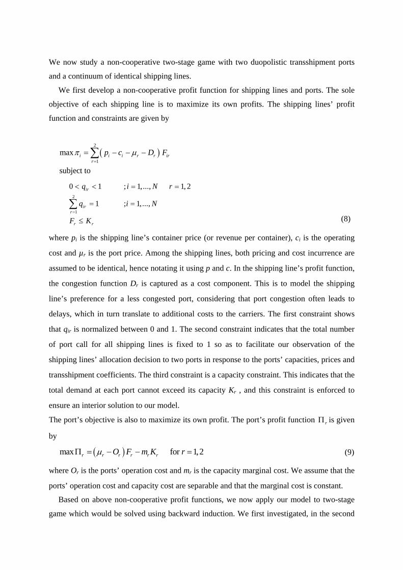
We now study a non-cooperative two-stage game with two duopolistic transshipment ports
and a continuum of identical shipping lines.
We first develop a non-cooperative profit function for shipping lines and ports. The sole
objective of each shipping line is to maximize its own profits. The shipping lines’ profit
function and constraints are given by
2
1
max
subject to
i i i r r irr
p c D F
2
1
0 1 ; 1,..., 1, 2
1 ; 1,...,
ir
irr
r r
q i N r
q i N
F K
(8)
where pi is the shipping line’s container price (or revenue per container), ci is the operating
cost and µr is the port price. Among the shipping lines, both pricing and cost incurrence are
assumed to be identical, hence notating it using p and c. In the shipping line’s profit function,
the congestion function Dr is captured as a cost component. This is to model the shipping
line’s preference for a less congested port, considering that port congestion often leads to
delays, which in turn translate to additional costs to the carriers. The first constraint shows
that qir is normalized between 0 and 1. The second constraint indicates that the total number
of port call for all shipping lines is fixed to 1 so as to facilitate our observation of the
shipping lines’ allocation decision to two ports in response to the ports’ capacities, prices and
transshipment coefficients. The third constraint is a capacity constraint. This indicates that the
total demand at each port cannot exceed its capacity Kr , and this constraint is enforced to
ensure an interior solution to our model.
The port’s objective is also to maximize its own profit. The port’s profit function r is given
by
max for 1,2r r r r r rO F m K r
(9)
where Or is the ports’ operation cost and mr is the capacity marginal cost. We assume that the
ports’ operation cost and capacity cost are separable and that the marginal cost is constant.
Based on above non-cooperative profit functions, we now apply our model to two-stage
game which would be solved using backward induction. We first investigated, in the second
stage, the shipping lines’ supply decision based upon the respective port’s capacity, price and
transshipment coefficient. Thereafter, we advance to the first stage to derive, in relation to the
shipping lines’ supply behaviour, a competitive port price. In addition, we apply comparative
static analysis on equilibrium shipping lines’ supply decision with respect to the concerned
parameters.
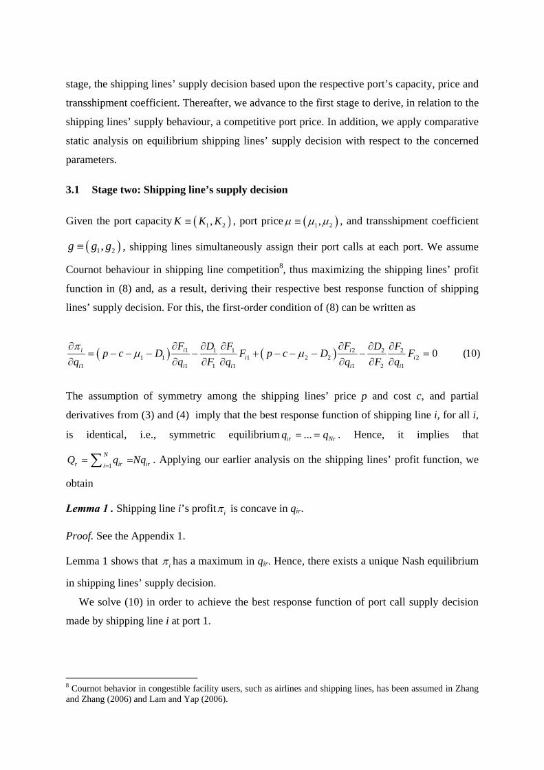
3.1 Stage two: Shipping line’s supply decision
Given the port capacity 1 2,K K K , port price 1 2, , and transshipment coefficient
1 2,g g g , shipping lines simultaneously assign their port calls at each port. We assume
Cournot behaviour in shipping line competition8, thus maximizing the shipping lines’ profit
function in (8) and, as a result, deriving their respective best response function of shipping
lines’ supply decision. For this, the first-order condition of (8) can be written as
1 21 1 2 21 1 1 2 2 2
1 1 1 1 1 2 1
0 (10)i i ii i
i i i i i
F FD F D Fp c D F p c D F
q q F q q F q
The assumption of symmetry among the shipping lines’ price p and cost c, and partial
derivatives from (3) and (4) imply that the best response function of shipping line i, for all i,
is identical, i.e., symmetric equilibrium ...ir Nrq q . Hence, it implies that
1
N
r ir iriQ q Nq
. Applying our earlier analysis on the shipping lines’ profit function, we
obtain
Lemma 1 . Shipping line i’s profit i is concave in qir.
Proof. See the Appendix 1.
Lemma 1 shows that i has a maximum in qir. Hence, there exists a unique Nash equilibrium
in shipping lines’ supply decision.
We solve (10) in order to achieve the best response function of port call supply decision
made by shipping line i at port 1.
8 Cournot behavior in congestible facility users, such as airlines and shipping lines, has been assumed in Zhang and Zhang (2006) and Lam and Yap (2006).
2 2 31 2 2
1 3 32 1
3 3 22 1 2 1 1 1 2 21 2 1 2
1 2 23 3 22 1 1 2 1 23
Ki
f g g g Nq
N g g
g g K p c g g g gf g g g g Ng g
N g g aN f g g g g N
(11)
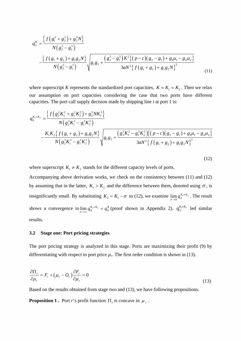
where superscript K represents the standardized port capacities, 1 2K K K . Then we relax
our assumption on port capacities considering the case that two ports have different capacities. The port call supply decision made by shipping line i at port 1 is:
1 2
2 2 2 2 3 22 1 1 2 2 1
1 3 2 3 22 1 1 2
3 2 3 22 1 1 2 2 1 1 1 2 21 2 1 2 1 2
1 2 23 2 3 2 22 1 1 2 1 2 1 23
K Ki
f g K g K g NKq
N g K g K
g K g K p c g g g gK K f g g g g Ng g
N g K g K aN f g g g g N
(12)
where superscript 1 2K K stands for the different capacity levels of ports.
Accompanying above derivation works, we check on the consistency between (11) and (12)
by assuming that in the latter, 1 2K K and the difference between them, denoted using , is
insignificantly small. By substituting 2 1K K to (12), we examine 1 210
lim K Kiq
. The result
shows a convergence to 1 21 1lim K K K
i iq q
(proof shown in Appendix 2). 1 2
2K Kiq led similar
results.
3.2 Stage one: Port pricing strategies
The port pricing strategy is analyzed in this stage. Ports are maximizing their profit (9) by
differentiating with respect to port price µr. The first order condition is shown in (13).
0r rr r r
r r
FF O
(13)
Based on the results obtained from stage two and (13), we have following propositions.
Proposition 1 . Port r’s profit function r is concave in r .
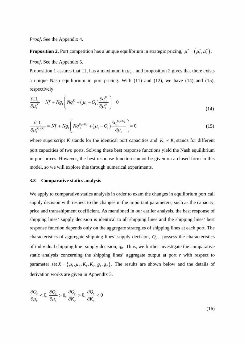
Proof. See the Appendix 4.
Proposition 2. Port competition has a unique equilibrium in strategic pricing, * * *1 2, .
Proof. See the Appendix 5.
Proposition 1 assures that r has a maximum in r , and proposition 2 gives that there exists
a unique Nash equilibrium in port pricing. With (11) and (12), we have (14) and (15),
respectively.
111 1 1 1
1 1
0K
K iiK K
qNf Ng Nq O
(14)
1 2
1 2
1 2
111 1 1 1
11
0K K
K K iiK K
qNf Ng Nq O
(15)
where superscript K stands for the identical port capacities and 1 2K K stands for different
port capacities of two ports. Solving these best response functions yield the Nash equilibrium
in port prices. However, the best response function cannot be given on a closed form in this
model, so we will explore this through numerical experiments.
3.3 Comparative statics analysis
We apply to comparative statics analysis in order to exam the changes in equilibrium port call
supply decision with respect to the changes in the important parameters, such as the capacity,
price and transshipment coefficient. As mentioned in our earlier analysis, the best response of
shipping lines’ supply decision is identical to all shipping lines and the shipping lines’ best
response function depends only on the aggregate strategies of shipping lines at each port. The
characteristics of aggregate shipping lines’ supply decision, rQ , possess the characteristics
of individual shipping line’ supply decision, qir. Thus, we further investigate the comparative
static analysis concerning the shipping lines’ aggregate output at port r with respect to
parameter set 1 2 1 2 1 2, , , , ,X K K g g . The results are shown below and the details of
derivation works are given in Appendix 3.
0,r
r
Q
0,r
s
Q
0,r
r
Q
K
0r
s
Q
K
(16)
As shown in (16) 9, shipping lines’ aggregate output at port r decreases with own port’s price
and increases with own port’s capacity. We obtain the below (17) and (18), the response of
transshipment coefficient to aggregate shipping lines’ output.
22
2 2 2 22 2
2
2
r r rr
r s sr rr r s s r s
r sr s
p c D DQ
g D DD DN g F g F g g
F FF F
(17)
22
2 2 2 22 2
2
2
s s sr
s s sr rr r s s r s
r sr s
p c D DQ
g D DD DN g F g F g g
F FF F
(18)
It can be implied that if the shipping lines’ profit margin at port r is bigger than the double
summation of port r’s total congestion delay cost, aggregate shipping lines’ output increases
with the transshipment coefficient, which means higher transshipment coefficient leads to a
more port calls from shipping lines. If not, total congestion delay cost overtakes profit
margin. On the other hand, as given in (18), if the competitor port has higher profit margin
than their overall congestion delay cost, shipping lines may assign more port call at
competitor port.
4. Ports collusion and social optimum
Thus far in this study, we had focused mainly on a non-cooperative game where every port
and shipping line makes independent decisions to maximize own profit. We now consider the
case of two ports cooperating on prices and capacities, and of all market players, two ports
and N-shipping line, cooperating to maximize the market profit to compare against the non-
cooperative model.
4.1 Ports collusion model
Considering the case in which the two ports decide their prices and capacities concurrently.
The profit function of ports collusion model is shown in below (19).
1 2 1 1 1 1 1 2 2 2 2 2maxr
O F m K O F m K
(19)
The first-order conditions for each port pricing from (19) is
9 This result is consistent with the comparative statics in Zhang and Zhang(2006) and Basso and Zhang(2007).
1 2 1 21 1 1 2 2
1 1 1
0F F
F O O
1 2 1 22 1 1 2 2
2 2 2
0F F
F O O
(20)
where 1 1 2 1F F . Therefore, 1 2 1 0 which means if there is no
boundary for maximum port price, the port price would reach infinity. This is due to our
assumption that shipping lines must call at both port (first constraint in (8)). Hence, compared
with the non-cooperative case, we can easily observe that the port collusion model yields
higher port price than the non-cooperative model. The result is intuitive that this case
becomes a monopoly market. Therefore, in this case of monopolistic cooperation, the ports
can have a free hand in escalating their prices (infinity) to maximize their profits. This
analysis would help better explain the competitive landscape and strategies among regionally
bounded terminal operators.
4.2 Social optimum model
We now consider a social optimum model that reflects cooperation among all players in the
game to maximize their combined profits. This is captured in the social-welfare function
(SW) given below:
2 2 2
, 1 1 1 1 1
maxr ir
N N
r i r r r r r r r irq
r i r i r
SW O F m K p c D F
(21)
A reduced form of (21) is presented by
1 2 1 1 1 1 1 2 2 2 2 2SW p c F F O D F m K O D F m K (22)
It is important to note that the port price disappears from (21) to give (22). This is because of
the internalization of the port price due to the equality between total port revenue and the sum
of shipping lines’ port cost. Therefore, there is no pricing stage in this model, but the supply
decision game among shipping lines is considered. The shipping lines’ supply decision in
social optimum model is characterized by first order condition below.
1 1 1 21 1 1 2 2
1 1 1 1 1
2 2 1 22
2 1 1 1
0
i i i i
i i i
F D F FSWO D F O D
q q F q q
D F F FF p c
F q q q
(23)
The standardized port capacities, K=K1=K2, give an explanation only to a port operation cost
which is the only factor to affect on supply decision compared to non-cooperative model,
hence relaxing this assumption to consider the different capacities of two ports, i.e. 1 2K K .
Solving (23) we can achieve the derived shipping lines’ supply decision below.
2 2 31 2 2
1 3 32 1
3 3 22 1 2 1 1 1 2 21 2 1 2
1 2 23 3 22 1 1 2 1 23
Ki SW
f g g g Nq
N g g
g g K p c g g g O g Of g g g g Ng g
N g g aN f g g Ng g
1 2
2 2 2 2 3 22 1 1 2 2 1
1 3 3 3 22 1 1 2
3 2 3 22 1 1 2 2 1 1 1 2 21 2 1 2 1 2
1 2 23 3 3 2 22 1 1 2 1 2 1 23
K Ki SW
f g K g K g NKq
N g K g K
g K g K p c g g g O g OK K f g g g g Ng g
N g K g K aN f g g g g N
(24)
where superscript SW stands for social welfare maximization. It depicts that in social
optimum model, the shipping lines’ decision in number of port calls seeks to minimize
congestion delay cost and port operation cost so as to maximize overall profits.
To better appreciate the model, we can perceive the stipulated conditions as a vertical
integration of shipping lines, where they extend their core businesses from liner shipping to
terminal operation, such as A.P.Moller-Maersk whose business scope is in container shipping
services and terminal operations. In this case, social optimum model explains the structure of
these carriers’ profit, where ports’ prices are internalized and ports’ demands are determined
by port operation cost, capacity and transshipment volume.
5. Numerical results
In addition to the derived functions for the shipping lines’ supply decision and the port
pricing, we further explore the comparative statics through a set of numerical experiments.
Firstly, we explain the effect on shipping lines’ supply decision conditional on differing port
prices between two ports while applying various levels of port capacities. Secondly, we show
the effect of transshipment coefficient on shipping lines’ supply decision while applying
various levels of port capacities. Thirdly, as it is not able to achieve the closed form of port
pricing stage, exploring the changes in equilibrium port prices with the changes in the
parameters. Lastly, we show the comparison results of social optimum model and non-
cooperative model in terms of shipping lines’ supply decision and market profits.
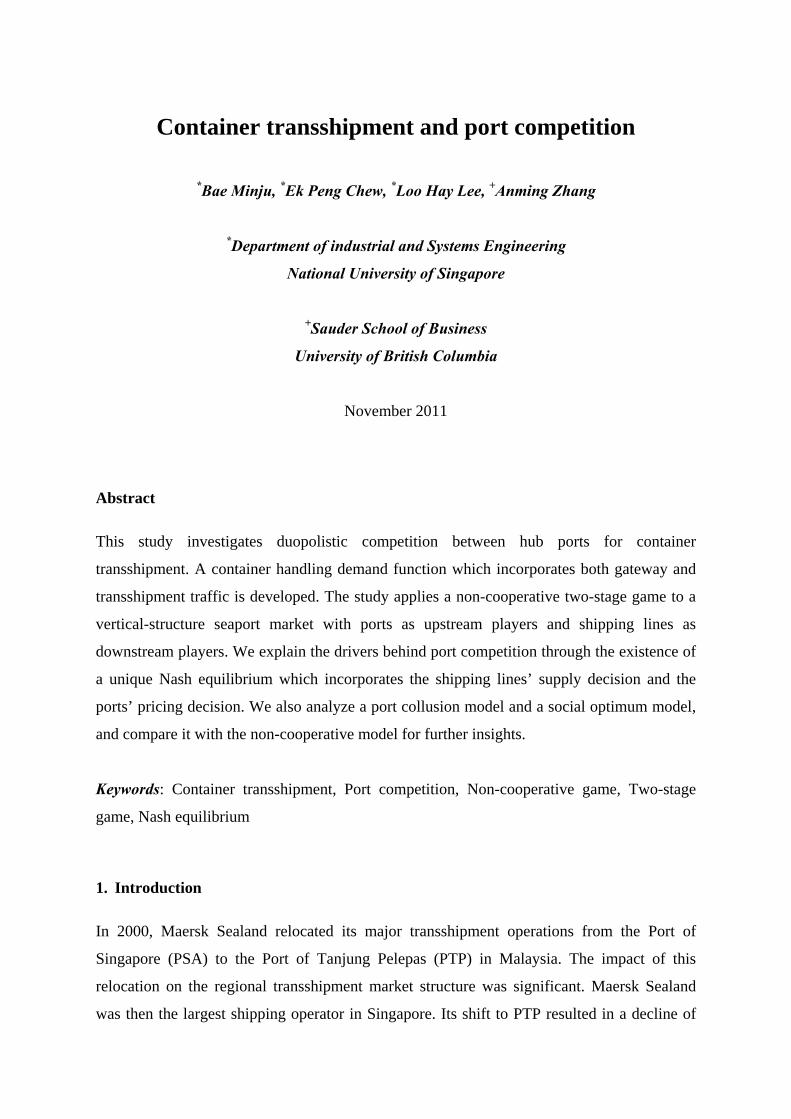
Figure 1 shows the shipping lines’ supply decision subjected to differing prices between
two equally-sized ports. As expected, similar port prices will yield an equal portion of port
calls to both ports. The portion of port calls to port 1 decreases as port 1’s price increases.
This implies that shipping lines are easily attracted by a cheaper port price. Another
important finding from Figure 1 is the combined effect of capacity and price level. Different
slope gradients were obtained when different port capacities were subjected to similar price
differentials (see K=4 and K=8.29). While capacity K=4 carried a gentle slope, the capacity
K=8.29 resulted in the steep slope. These results showed that when the both ports’ capacities
are large, a marginal difference between two port prices is sufficient to drive significant
demand to the cheaper port. In contrast, when both ports’ capacities are small, the shift of
demand becomes inelastic to the difference in port prices. Therefore, it is reasonable to
assume that the congestion effect associated with a small port capacity offsets the price
difference between ports, and that a large port capacity offsets the congestion effect and
hence amplifies the effect of price difference.
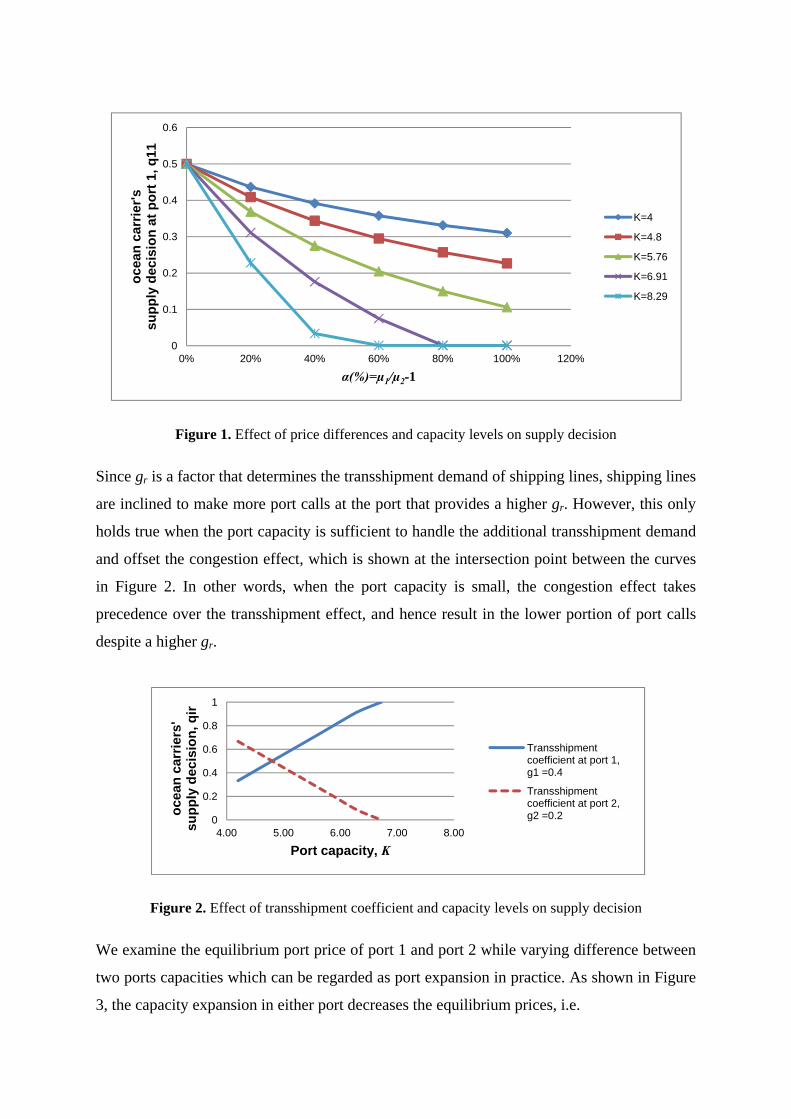
Figure 1. Effect of price differences and capacity levels on supply decision
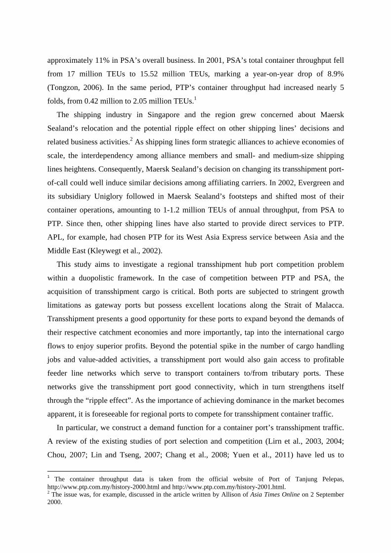
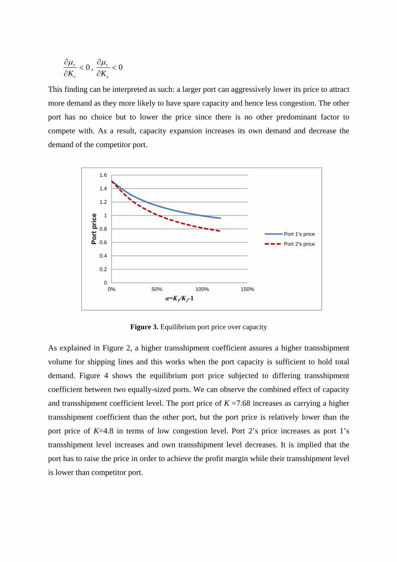
Since gr is a factor that determines the transshipment demand of shipping lines, shipping lines
are inclined to make more port calls at the port that provides a higher gr. However, this only
holds true when the port capacity is sufficient to handle the additional transshipment demand
and offset the congestion effect, which is shown at the intersection point between the curves
in Figure 2. In other words, when the port capacity is small, the congestion effect takes
precedence over the transshipment effect, and hence result in the lower portion of port calls
despite a higher gr.
Figure 2. Effect of transshipment coefficient and capacity levels on supply decision
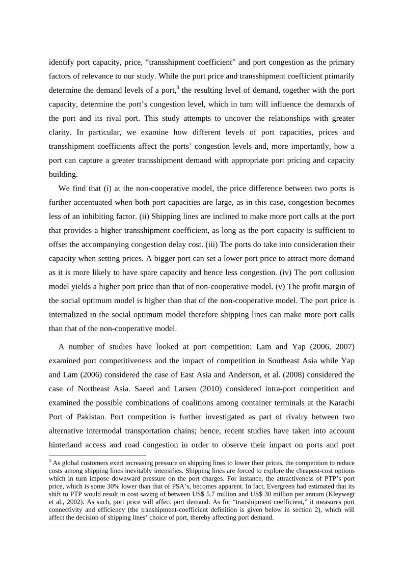
We examine the equilibrium port price of port 1 and port 2 while varying difference between
two ports capacities which can be regarded as port expansion in practice. As shown in Figure
3, the capacity expansion in either port decreases the equilibrium prices, i.e.
0
0.1
0.2
0.3
0.4
0.5
0.6
0% 20% 40% 60% 80% 100% 120%
oce
an c
arri
er's
su
pp
ly d
ecis
ion
at
po
rt 1
, q11
α(%)=µ1/µ2-1
K=4
K=4.8
K=5.76
K=6.91
K=8.29
0
0.2
0.4
0.6
0.8
1
4.00 5.00 6.00 7.00 8.00
oce
an c
arri
ers'
su
pp
ly d
ecis
ion
, qir
Port capacity, K
Transshipment coefficient at port 1, g1 =0.4
Transshipment coefficient at port 2, g2 =0.2
0r
rK
, 0r
sK
This finding can be interpreted as such: a larger port can aggressively lower its price to attract
more demand as they more likely to have spare capacity and hence less congestion. The other
port has no choice but to lower the price since there is no other predominant factor to
compete with. As a result, capacity expansion increases its own demand and decrease the
demand of the competitor port.
Figure 3. Equilibrium port price over capacity
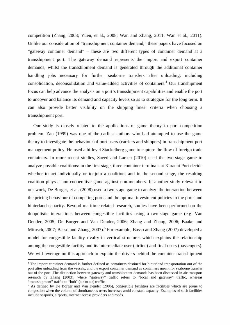
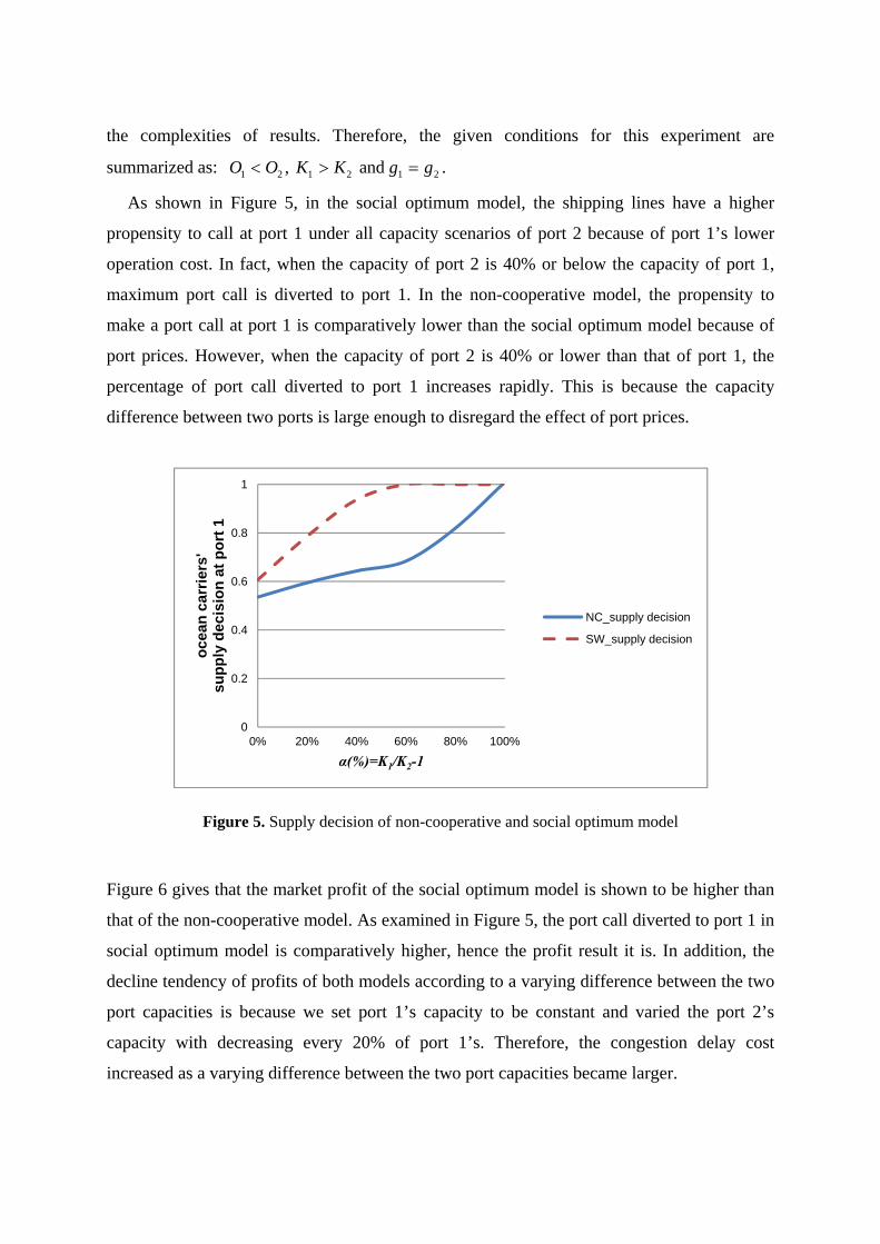
As explained in Figure 2, a higher transshipment coefficient assures a higher transshipment
volume for shipping lines and this works when the port capacity is sufficient to hold total
demand. Figure 4 shows the equilibrium port price subjected to differing transshipment
coefficient between two equally-sized ports. We can observe the combined effect of capacity
and transshipment coefficient level. The port price of K =7.68 increases as carrying a higher
transshipment coefficient than the other port, but the port price is relatively lower than the
port price of K=4.8 in terms of low congestion level. Port 2’s price increases as port 1’s
transshipment level increases and own transshipment level decreases. It is implied that the
port has to raise the price in order to achieve the profit margin while their transshipment level
is lower than competitor port.
0
0.2
0.4
0.6
0.8
1
1.2
1.4
1.6
0% 50% 100% 150%
Po
rt p
rice
α=K1/K2-1
Port 1's price
Port 2's price
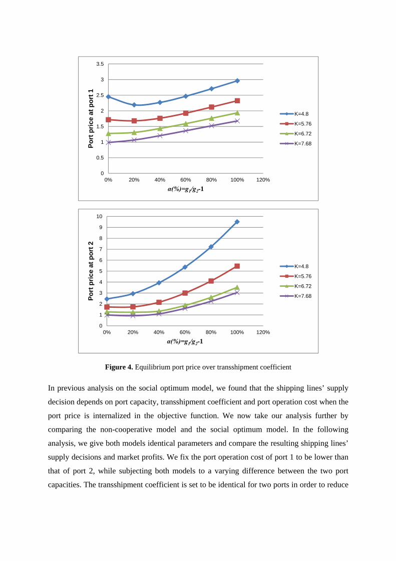
Figure 4. Equilibrium port price over transshipment coefficient
In previous analysis on the social optimum model, we found that the shipping lines’ supply
decision depends on port capacity, transshipment coefficient and port operation cost when the
port price is internalized in the objective function. We now take our analysis further by
comparing the non-cooperative model and the social optimum model. In the following
analysis, we give both models identical parameters and compare the resulting shipping lines’
supply decisions and market profits. We fix the port operation cost of port 1 to be lower than
that of port 2, while subjecting both models to a varying difference between the two port
capacities. The transshipment coefficient is set to be identical for two ports in order to reduce
0
0.5
1
1.5
2
2.5
3
3.5
0% 20% 40% 60% 80% 100% 120%
Po
rt p
rice
at
po
rt 1
α(%)=g1/g2-1
K=4.8
K=5.76
K=6.72
K=7.68
0
1
2
3
4
5
6
7
8
9
10
0% 20% 40% 60% 80% 100% 120%
Po
rt p
rice
at
po
rt 2
α(%)=g1/g2-1
K=4.8
K=5.76
K=6.72
K=7.68
the complexities of results. Therefore, the given conditions for this experiment are
summarized as: 1 2 1 2 1 2 , and O O K K g g .
As shown in Figure 5, in the social optimum model, the shipping lines have a higher
propensity to call at port 1 under all capacity scenarios of port 2 because of port 1’s lower
operation cost. In fact, when the capacity of port 2 is 40% or below the capacity of port 1,
maximum port call is diverted to port 1. In the non-cooperative model, the propensity to
make a port call at port 1 is comparatively lower than the social optimum model because of
port prices. However, when the capacity of port 2 is 40% or lower than that of port 1, the
percentage of port call diverted to port 1 increases rapidly. This is because the capacity
difference between two ports is large enough to disregard the effect of port prices.
Figure 5. Supply decision of non-cooperative and social optimum model
Figure 6 gives that the market profit of the social optimum model is shown to be higher than
that of the non-cooperative model. As examined in Figure 5, the port call diverted to port 1 in
social optimum model is comparatively higher, hence the profit result it is. In addition, the
decline tendency of profits of both models according to a varying difference between the two
port capacities is because we set port 1’s capacity to be constant and varied the port 2’s
capacity with decreasing every 20% of port 1’s. Therefore, the congestion delay cost
increased as a varying difference between the two port capacities became larger.
0
0.2
0.4
0.6
0.8
1
0% 20% 40% 60% 80% 100%
oce
an c
arri
ers'
su
pp
ly d
ecis
ion
at
po
rt 1
α(%)=K1/K2-1
NC_supply decision
SW_supply decision
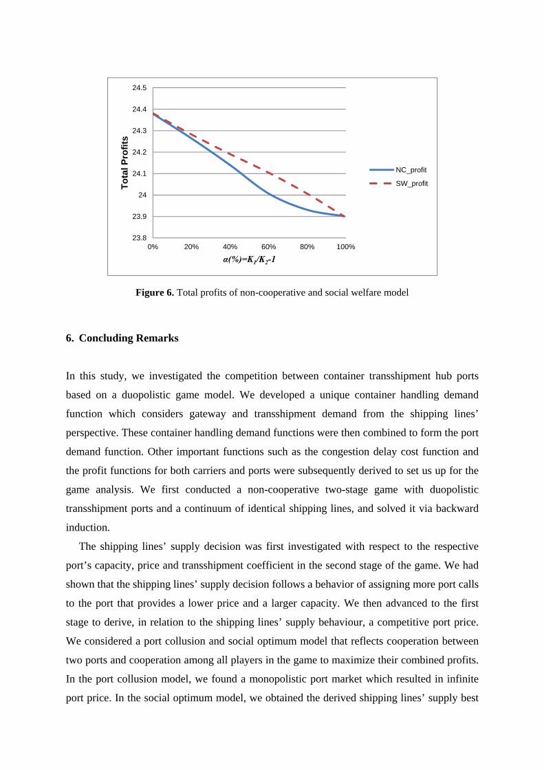
Figure 6. Total profits of non-cooperative and social welfare model
6. Concluding Remarks
In this study, we investigated the competition between container transshipment hub ports
based on a duopolistic game model. We developed a unique container handling demand
function which considers gateway and transshipment demand from the shipping lines’
perspective. These container handling demand functions were then combined to form the port
demand function. Other important functions such as the congestion delay cost function and
the profit functions for both carriers and ports were subsequently derived to set us up for the
game analysis. We first conducted a non-cooperative two-stage game with duopolistic
transshipment ports and a continuum of identical shipping lines, and solved it via backward
induction.
The shipping lines’ supply decision was first investigated with respect to the respective
port’s capacity, price and transshipment coefficient in the second stage of the game. We had
shown that the shipping lines’ supply decision follows a behavior of assigning more port calls
to the port that provides a lower price and a larger capacity. We then advanced to the first
stage to derive, in relation to the shipping lines’ supply behaviour, a competitive port price.
We considered a port collusion and social optimum model that reflects cooperation between
two ports and cooperation among all players in the game to maximize their combined profits.
In the port collusion model, we found a monopolistic port market which resulted in infinite
port price. In the social optimum model, we obtained the derived shipping lines’ supply best
23.8
23.9
24
24.1
24.2
24.3
24.4
24.5
0% 20% 40% 60% 80% 100%
To
tal P
rofi
ts
α(%)=K1/K2-1
NC_profit
SW_profit
response function that showed that the shipping lines’ decision in number of port calls seeks
to minimize the ports’ operation costs and congestion delay costs so as to maximize overall
profits.
To further our observation of the Nash equilibrium point, numerical experiments are
conducted. We first found that price difference between two ports is further accentuated when
both port capacities are large, as in this case, congestion becomes less of an inhibiting factor.
Next, shipping lines are inclined to make more port calls at the port that provides a higher gr ,
as long as the port capacity is sufficient to offset the accomapnying congestion delay cost. In
other words, when the port capacity is small, the congestion delay cost takes precedence over
the transshipment volume, and hence result in a lower number of port calls despite a higher
gr. We had shown that ports do take into consideration their capacity when setting prices. A
bigger port can set a lower port price to attract more demand as they more likely to have
spare capacity and hence less congestion. And finally, the result of comparing non-
cooperative model against social optimum model showed that the internalized port price
paved the way for social optimum model focusing on minimizing overall cost so as to
maximize the market profit. The non-cooperative model, on the other hand, is restricted by
port price, hence resulting less profit margin.
In the main, this study may provide further insights to the shipping lines’ behaviour and
the characteristics of transshipment demand. Such insights can serve as useful information to
the port operators when optimizing their port pricing strategies. Furthermore, this study can
be improved with nonlinear demand function to be shown more obvious behaviour of
shipping lines’ preference on their supply decision. The tradeoffs of the congestion cost and
transshipment benefits can be shown clearly in nonlinear demand function model.
Asymmetric shipping lines’, unlikely this study only considered the symmetric conditions of
shipping lines’, would also be taken into account in the future study. The shift of port call
supply decision can be determined by shipping lines’ own operating cost and price to the
consignors which can affect the marginal profit of shipping lines’.
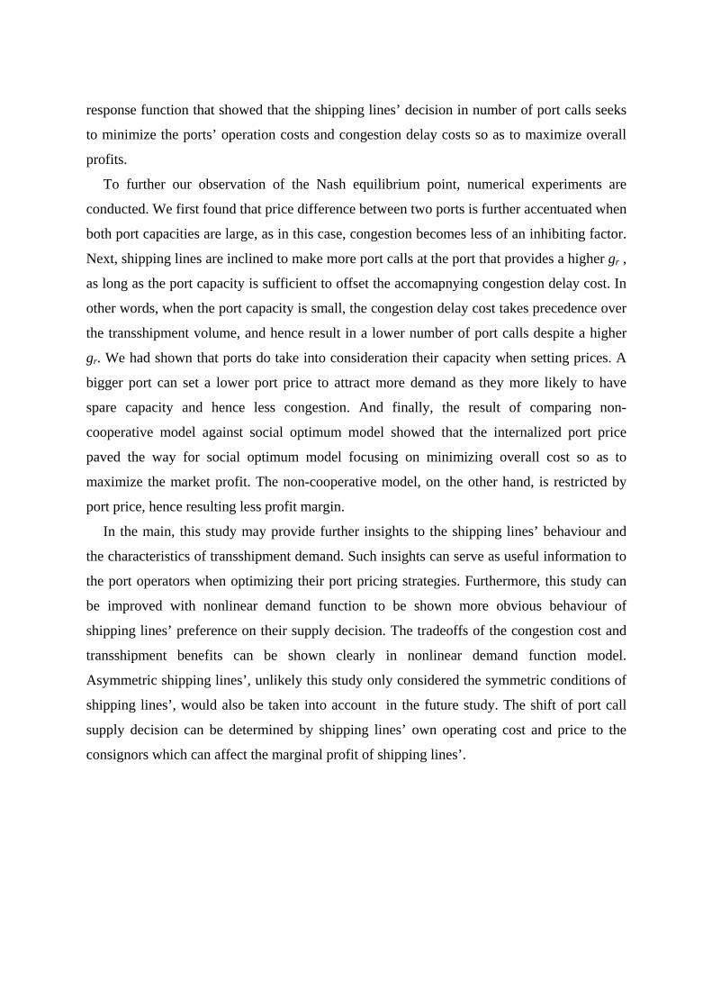
Appendix
1. Proof of Lemma 1
From (3),(4),(6),(7), we obtain
2 22 2 21 21 1 1 1 2 2 2 2
1 22 2 21 1 1 1 2 1 1 11 1 2
2 22 22 21 1 2 2
1 1 1 2 2 22 21 21 2
22 21 11 12
1 1
2 2
2 2
2
i i ii i
i i i i i ii
i i
i
F FD F D F D F D FF F
F q q q F q q qq F F
D D D DNg Ng F Ng Ng F
F FF F
D Dg N N F g
F F
22 22 22 22
2 2
2 0i
D DN N F
F F
(A.1)
Therefore, i is concave in irq .
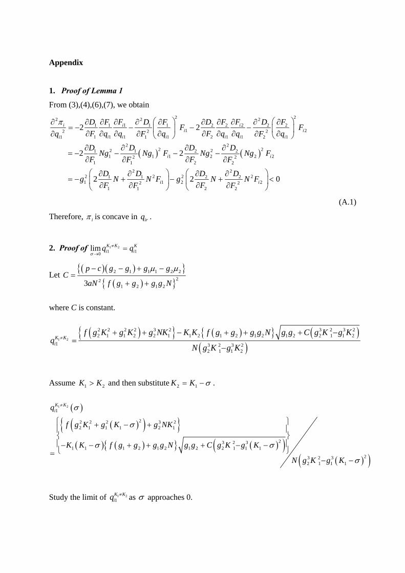
2. Proof of 1 21 10
lim K K Ki iq q
Let
2 1 1 1 2 2
221 2 1 23
p c g g g gC
aN f g g g g N
where C is constant.
1 2
2 2 2 2 3 2 3 2 3 22 1 1 2 2 1 1 2 1 2 1 2 1 2 2 1 1 2
1 3 2 3 22 1 1 2
K Ki
f g K g K g NK K K f g g g g N g g C g K g Kq
N g K g K
Assume 1 2K K and then substitute 2 1K K .
1 21
22 2 2 3 22 1 1 1 2 1
23 2 31 1 1 2 1 2 1 2 2 1 1 1
23 2 32 1 1 1
K Kiq
f g K g K g NK
K K f g g g g N g g C g K g K
N g K g K
Study the limit of 1 21K Kiq as approaches 0.
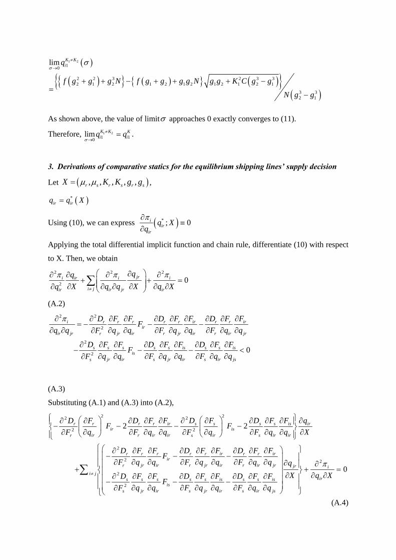
1 21
0
2 2 3 2 3 32 1 2 1 2 1 2 1 2 1 2 1
3 32 1
lim K Kiq
f g g g N f g g g g N g g K C g g
N g g
As shown above, the value of limit approaches 0 exactly converges to (11).
Therefore,
1 21 1
0lim K K K
i iq q
.
3. Derivations of comparative statics for the equilibrium shipping lines’ supply decision
Let , , , , ,r s r s r sX K K g g ,
*ir irq q X
Using (10), we can express * ; 0iir
ir
q Xq
Applying the total differential implicit function and chain rule, differentiate (10) with respect
to X. Then, we obtain
2 2 2
20jri ir i i
i j ir jr irir
X q q X q Xq
(A.2)
2 2
2
2
20
i ir irr r r r r r rir
ir jr jr ir r jr ir r ir jrr
s s s s s is s s isis
jr ir s jr ir s ir jss
F FD F F D F D FF
q q q q F q q F q qF
D F F D F F D F FF
q q F q q F q qF
(A.3)
Substituting (A.1) and (A.3) into (A.2),
2 222
2 2
2
2
2
2
2 2ir s s s s is irr r r rir is
ir r ir ir ir s ir irr s
ir irr r r r r r rir
jr ir r jr ir r ir jrr
s s
js
F D F D F F qD F D FF F
q F q q q F q q XF F
F FD F F D F D FF
q q F q q F q qF
D F
qF
2
0jr i
i jirs s s is s s is
isr ir s jr ir s ir js
q
X q XF D F F D F FF
q F q q F q q
(A.4)
From the properties of demand and congestion delay cost function in (3) and (4), the (A.4)
can be expressed as:
22 2
2
22
2
22 2
2 2
22 2
2
22 2
2
2
2
2
0
2
2
r rr ir r
rr ir
s ss is s s
ss
r rr ir r r
jrrr i
i j irs ss is s s
ss
rr ir
r
D DNg F Ng
FF q
XD DNg F Ng g
FF
D DN g F Ng g
qFF
X q XD DN g F Ng g
FF
DN g F
F
2
22 2
2
22 2
2
22 2
1 2
22 2
2
2
2
rr
r ir
s ss is s s
ss
r r rr ir r r r r
r rr irN
s s si s is s s s s
s ss
r rr ir
rr
DNg
F q
XD DN g F Ng g
FF
D D DN g F Ng g Ng g
F FF q
XD D DN g F Ng g Ng g
F FF
D DN g F N
FF
2
22 2
2
0
2
r r
ir i
irs ss is s s
ss
g gq
X q XD DN g F Ng g
FF
Finally,
22 2
2 2
22 2
2
2
0
2
r rr ir r r
rr ir
irs ss is s s
ss
D DN g F Ng g
FF Q
X q XD DN g F Ng g
FF
(A.5)
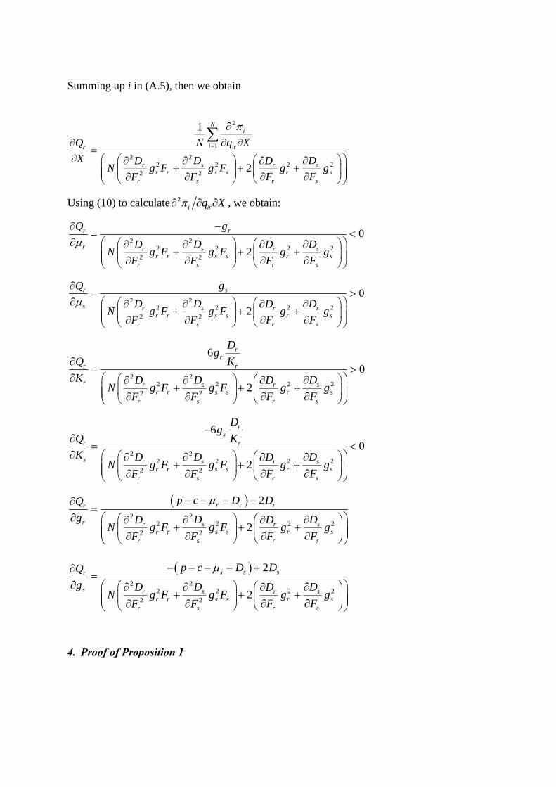
Summing up i in (A.5), then we obtain
2
1
222 2 2 2
2 2
1
2
Ni
i irr
s sr rr r s s r s
r sr s
N q XQ
X D DD DN g F g F g g
F FF F
Using (10) to calculate 2i irq X , we obtain:
222 2 2 2
2 2
0
2
r r
r s sr rr r s s r s
r sr s
Q g
D DD DN g F g F g g
F FF F
222 2 2 2
2 2
0
2
sr
s s sr rr r s s r s
r sr s
gQ
D DD DN g F g F g g
F FF F
222 2 2 2
2 2
6
0
2
rr
r r
r s sr rr r s s r s
r sr s
Dg
Q K
K D DD DN g F g F g g
F FF F
222 2 2 2
2 2
6
0
2
rs
r r
s s sr rr r s s r s
r sr s
Dg
Q K
K D DD DN g F g F g g
F FF F
22
2 2 2 22 2
2
2
r r rr
r s sr rr r s s r s
r sr s
p c D DQ
g D DD DN g F g F g g
F FF F
22
2 2 2 22 2
2
2
s s sr
s s sr rr r s s r s
r sr s
p c D DQ
g D DD DN g F g F g g
F FF F
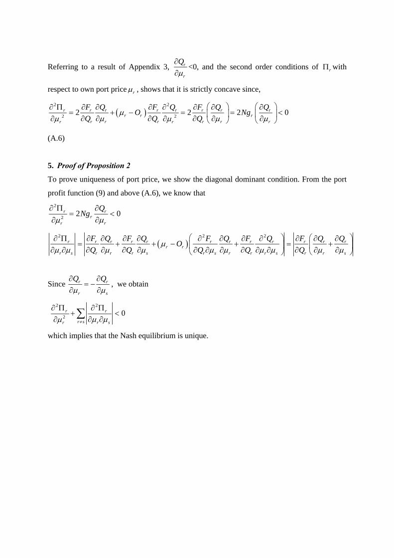
4. Proof of Proposition 1
Referring to a result of Appendix 3, r
r
Q
<0, and the second order conditions of r with
respect to own port price r , shows that it is strictly concave since,
2 2
2 22 2 2 0r r r r r r r r
r r rr r r r r rr r
F Q F Q F Q QO Ng
Q Q Q
(A.6)
5. Proof of Proposition 2
To prove uniqueness of port price, we show the diagonal dominant condition. From the port
profit function (9) and above (A.6), we know that
2
22 0r r
rrr
QNg
2 2 2
r r r r r r r r r r r rr r
r s r r r s r s r r r s r r s
F Q F Q F Q F Q F Q QO
Q Q Q Q Q
Since r r
r s
Q Q
, we obtain
2 2
20 r r
r s r sr
which implies that the Nash equilibrium is unique.
References
Allison, T., “A new era in Asian shipping”, Asia Times Online: Southeast Asia, 2 September
2000, retrieved from http://www.atimes.com/se-asia/BI02Ae06.html, 3 April 2010.
Anderson, C.M., Park, Y.A., Chang, Y.T., Yang, C.H., Lee, T.W. and Luo, M. (2008), “A
game-theoretic analysis of competition among container port hubs: The case of Busan and
Shanghai”, Maritime Policy & Management, 35(1), 5-26.
Baake, P. and Mitusch, K. (2007), “Competition with congestible networks”, Journal of
Economics, 91(2), 151-176.
Basso, L.J. and Zhang, A. (2007), “Congestible facility rivalry in vertical structures”, Journal
of Urban Economics, 61, 218-237.
Chang, Y.T, Lee, S.Y. and Tongzon, J.L. (2008), “Port selection factors by shipping lines:
Different perspectives between trunk liners and feeder service providers”, Marine Policy,
32(6), 877-885.
Chou, C.C. (2007), “A fuzzy MCDM method for solving marine transshipment container port
selection problems”, Applied Mathematics and Computation, 186, 435-444.
De Borger, B. and Van Dender, K. (2006), “Prices, capacities and service levels in a
congestible Bertrand duopoly”, Journal of Urban Economics, 60, 264-283.
De Borger, B., Proost, S. and Van Dender, K. (2008), “Private port pricing and public
investment in port and hinterland capacity”, Journal of Transport Economics and Policy,
42(3), 527-561.
Frankel, E.G. (2002), “The challenge of container transshipment in the Caribbean”, The
International Association of Maritime Economists (IAME) Annual Conference 2002
Conference Proceedings, Panama.
Kleywegt, A.T., Goh, M.L., Wu, G.Y. and Zhang, H.W. (2002), “Competition between the
ports of Singapore and Malaysia”, Technical Report, The Logistics Institute, Georgia Tech,
and The Logistics Institute-Asia Pacific, National University of Singapore.
Lam, J.S.L. and Yap, W.Y. (2006), “A measurement and comparison of cost competitiveness
of container ports in Southeast Asia”, Transportation, 33, 641-654.
Lam, J.S.L and Yap, W.Y. (2007), “Competition for transshipment containers by major ports
in Southeast Asia: Slot capacity analysis”, 2007 International Conference on Logistics,
Shipping and Port management, Taiwan.
Lin, L.C. and Tseng, C.C. (2007), “Operational performance evaluation of major container
ports in the Asia-Pacific Region”, Maritime Policy and Management, 32(6), 535-551.
Lirn, T.C., Thanopoulou, H.A. and Bersesford, A.K.C. (2003), “Transshipment port selection
and decision-making behavior: Analysing the Taiwanese case”, International Journal of
Logistics: Research and Applications, 6(4), 229-244.
Lirn, T.C, Thanopoulou, H.A. and Beresford, A.K.C. (2004), “An application of AHP on
transshipment port selection: A global perspective”, Maritime Economics and Logistics, 6,
70-91.
Saeed, N. and Larsen, O.I. (2010), “An application of cooperative game among container
terminals of one port”, European Journal of Operational Research, 203(2), 392-403.
Tongzon, J.L. (2006), “Privatization: The port of Singapore experience”, Project Paper of
Asia Research Centre, Murdoch University.
Van Dender, K. (2005), “Duopoly prices under congested access”, Journal of Regional
Science, 45, 343-362.
Wan, Y. and Zhang, A. (2011), “Urban road congestion and port competition”, Journal of
Transport Economics and Policy, forthcoming.
Wan, Y., Zhang, A. and Yuen, A.C.L (2011), “Urban road congestion, capacity expansion
and port competition: Empirical analysis of U.S. container ports”, Working paper.
Yap, W.Y. and Lam, J.S.L. (2006), “Competition dynamics between container ports in East
Asia”, Transportation Research Part A, 40, 35-51.
Yuen, A.C.L., Basso, L.J. and Zhang, A. (2008), “Effects of gateway congestion pricing on
optimal road pricing and hinterland”, Journal of Transport Economics and Policy, 42(3),
495-526.
Yuen, A.C.L., Zhang, A. and Cheung, W. (2011), “Port Competitiveness from the users’
perspective: An AHP analysis of major container ports in China and its neighboring
countries”, Research in Transport Economics, forthcoming.
Zan, Y. (1999), “Analysis of container port policy by the reaction of an equilibrium shipping
market”, Maritime Policy & Management, 26(4), 369-381.
Zhang, A. (2003), “Analysis of an international air cargo hub: The case of Hong Kong”,
Journal of Air Transport Management, 9, 123-138.
Zhang, A. and Zhang, Y. (2006), “Airport capacity and congestion when carriers have market
power”, Journal of Urban Economics, 60, 229-247.
Zhang, A. (2008), “The impact of hinterland access conditions on rivalry between ports”,
OECD/ITF discussion paper 2008-8, Paris.