Embed Size (px)
Citation preview

Contents
7 Software Systems for Linear Algebra Problems 5317.1 Difference Between Solving a Small Problem By Hand
and Scientific Computing Using a Computer . . . . . . 5317.2 How to Enter Vectors and Matrices in MATLAB . . . . 5337.3 Illustrative Numerical Examples . . . . . . . . . . . . . 5387.4 References . . . . . . . . . . . . . . . . . . . . . . . . . 552
i

ii
Chapter 7
Software Systems for LinearAlgebra Problems
This is Chapter 7 of “Sophomore Level Self-Teaching Web-book for Computational and Algorithmic Linear Algebra andn-Dimensional Geometry” by Katta G. Murty.
Nowadays there are several commercially available and highly pop-ular software systems for solving the problems discussed in previouschapters. Among them the best known are: MATLAB, EXCEL, MATH-EMATICA, MAPLE, and MACAULAY. We will provide illustarativenumerical examples of how to solve these problems using MATLAB(this name is derived from Matrix Laboratory) in this chapter. Forusing the other software systems, see the references cited on them.
7.1 Difference Between Solving a Small
Problem By Hand and Scientific Com-
puting Using a Computer
When we solve small numerical problems by hand, we always use exactarithmetic, so all the numbers in the various stages of the work areexactly what they are supposed to be (for example, a fraction like “1/3”
531
532 Ch. 7. Software Systems
is maintained as it is). Hand computation is not feasible for large sizeproblems encountered in applications. Such large problems are usuallysolved using a software package on a digital computer.
Digital computation uses finite precision arithmetic, not exactarithmetic; for example a fraction like “1/3” is rounded to 0.3333 or0.3 . . . 3 depending on the number of significant digits of precisionmaintained, introducing a small rounding error. These roundingerrors abound in scientific computation, and they accumulate duringthe course of computation. So results obtained in digital computationusually contain some rounding errors, and may only be approximatelycorrect. These errors make it nontrivial to implement many of thealgorithms discussed in earlier chapters to get answers of reasonableprecision. That’s why detailed descriptions of numerical implementa-tions of algorithms are very different and much more complicated thantheir mathematical descriptions given in earlier chapters.
As an example consider the GJ pivotal method for solving a systemof linear equations discussed in Section 1.16. Under exact arithmetic,we know that a redundant constraint in the system corresponds to a“0 = 0” equation in the final tableau and vice versa. However, underfinite precision arithmetic some of the “0” entries in it may becomenonzero numbers of hopefully small absolute value. So, what is actu-ally a “0 = 0” equation in the final tableau, may in reality become anequation with nonzero entries of small absolute value, and it is verydifficult to decide whether it is a redundant equation or not. In com-puter implementations, one difficult question faced at every stage iswhether a nonzero entry of small absolute value is actually a nonzeroentry, or a zero entry that has become nonzero due to rounding erroraccumulation. A practical rule that is often used selects a small pos-itive tolerance, and replaces any entry in the tableau whose absolutevalue is less than this tolerance by zero. Under such a rule, we can onlyconclude that a “0 = 0” equation in the final tableau is redundant toworking precision.
In the same way, when a square matrix has a determinant of verysmall absolute value, using finite precision arithmetic it is very difficultto decide whether it is actually nonsingular or singular, and softwaresystems will conclude that this matrix is singular to working precision.
7.2 Vectors and Matrices 533
Similarly while the definitions of linear independence or dependenceof a set of vectors and its rank defined in Chapter 4 are conceptuallyprecise and mathematically unambiguous under exact arithmetic, usingfinite precision arithmetic they can only be determined correct to theworking precision.
Numerical analysts have developed a variety of techniques to reducethe effects of rounding errors, some of these like partial pivoting orcomplete pivoting for pivot element selection are discussed very brieflyin Chapter 1. As a detailed discussion of these techniques is beyondthe scope of this book, the interested reader should refer to books inthat area (for example, see Gill, Murray, Wright[4.1]).
We will see the effects of rounding errors in some of the illustrativenumerical examples given below.
7.2 How to Enter Vectors and Matrices
in MATLAB
First you need to begin a MATLAB session. It should be noted thatthere are many versions of MATLAB in the market, and input prompts,and error and warning messages may vary from version to version. Also,different computer systems may have different commands for initiatinga MATLAB session on their system.
After getting the MATLAB prompt, if you want to enter a rowvector, a = (1, 6, 7,−9) say, type
a = [1 6 7 −9] or a = [1, 6, 7, −9]
with a blank space or a comma (,) between entries, and MATLABresponds with
a = 1 6 7 −9.
To enter the same vector as a column vector, type
a = [1, 6, 7, −9]’ or a = [1 6 7 −9]’ or a = [1; 6; 7; −9]
and MATLAB responds with
534 Ch. 7. Software Systems
a = 167
−9
To supress the system’s response, a semicolon (;) is placed as thelast character of the expression. For example, after typing a = [1, 6,7, −9]; MATLAB responds with a new line awaiting a new command.
MATLAB also lets one place several expressions on one line, a linebeing terminated by pressing the Enter button on the computer. In thiscase, each expression is separated by either a comma (,) or a semicolon(;). The comma results in the system echoing the output; the semicolonsupresses it. For example, by typing
a = [1, 2, 6, 9], c = [2, −3, 1, −4]
the system responds with
a = 1 2 6 9c = 2 −3 1 −4.
Matrices are entered into MATLAB row by row, with rows sepa-rated by either semicolons, or by pressing Enter button on the com-puter. For example, to enter the matrix
A =
(10 −2 40 8 −7
)
type A = [10, −2, 4; 0, 8, −7]
or typeA = [ 10 −2 4
0 8 −7 ]using Enter to indicate theend of 1st row
or typeA = [ 10 −2 4; . . .
0 8 −7 ]the . . . called ellipses isa continuation of a MAT-LAB expression to next line.Used to create more read-able code.
7.2 Vectors and Matrices 535
MATLAB has very convenient ways to address the entries of a ma-trix. For example, to display the (2, 3) entry in the above matrix Atype A(2, 3), to display 2nd column of A type A(:, 2), and todisplay 2nd row of A type A(2, :).
Some of the commands used for special matrices are:
eye(n) identity matrix of order ndiag([a1 a2 . . . an]) diagonal matrix with diagonal entries
a1, . . . , an
zeros(m, n) zero matrix of order m × nzero(n) zero matrix of order n × n
A′ transpose of matrix A
If B is a square matrix defined in MATLAB, diag(B) returns thediagonal elements of B. To see the contents of a vector or matrix Adefined earlier, just type A and MATLAB responds by displayingit.
The arithmetic operators to perform addition, subtraction, multi-plication, division, and exponentiation are: +, −, *, /, ˆ respec-tively. As an example, suppose the vectors x = (1, 0, 0), y = (0, 1, 0),z = (0, 0, 1) have been defined earlier. If you type 2 ∗x+3 ∗ y − 6 ∗ zMATLAB responds with
ans = 2 3 −6.
If you type w = 2 ∗ x + 3 ∗ y − 6 ∗ z MATLAB responds with
w = 2 3 −6.
If you type an arithmetical expression that is not defined, for ex-ample x+y′ with x, y as defined above (i.e., the sum of a row vectorand a column vector), MATLAB yields the warning
???Error using =⇒ +Matrix dimensions must agree.
Other arithmetical operations on matrices and vectors can be de-fined in MATLAB in the same way. Here are some MATLAB com-mands that we will use, and the outputs they produce. For a morecomplete list of MATLAB commands, see the MATLAB references
536 Ch. 7. Software Systems
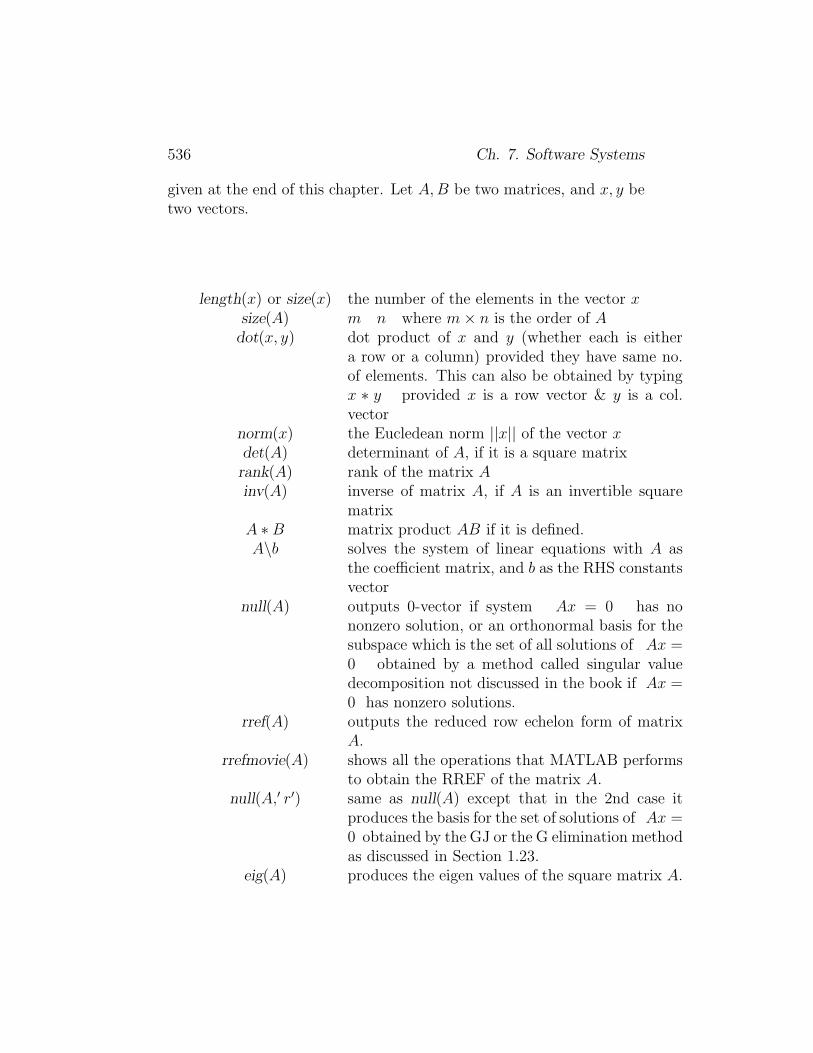
given at the end of this chapter. Let A, B be two matrices, and x, y betwo vectors.
length(x) or size(x) the number of the elements in the vector xsize(A) m n where m × n is the order of A
dot(x, y) dot product of x and y (whether each is eithera row or a column) provided they have same no.of elements. This can also be obtained by typingx ∗ y provided x is a row vector & y is a col.vector
norm(x) the Eucledean norm ||x|| of the vector xdet(A) determinant of A, if it is a square matrixrank(A) rank of the matrix Ainv(A) inverse of matrix A, if A is an invertible square
matrixA ∗ B matrix product AB if it is defined.A\b solves the system of linear equations with A as
the coefficient matrix, and b as the RHS constantsvector
null(A) outputs 0-vector if system Ax = 0 has nononzero solution, or an orthonormal basis for thesubspace which is the set of all solutions of Ax =0 obtained by a method called singular valuedecomposition not discussed in the book if Ax =0 has nonzero solutions.
rref(A) outputs the reduced row echelon form of matrixA.
rrefmovie(A) shows all the operations that MATLAB performsto obtain the RREF of the matrix A.
null(A,′ r′) same as null(A) except that in the 2nd case itproduces the basis for the set of solutions of Ax =0 obtained by the GJ or the G elimination methodas discussed in Section 1.23.
eig(A) produces the eigen values of the square matrix A.
7.2 Vectors and Matrices 537
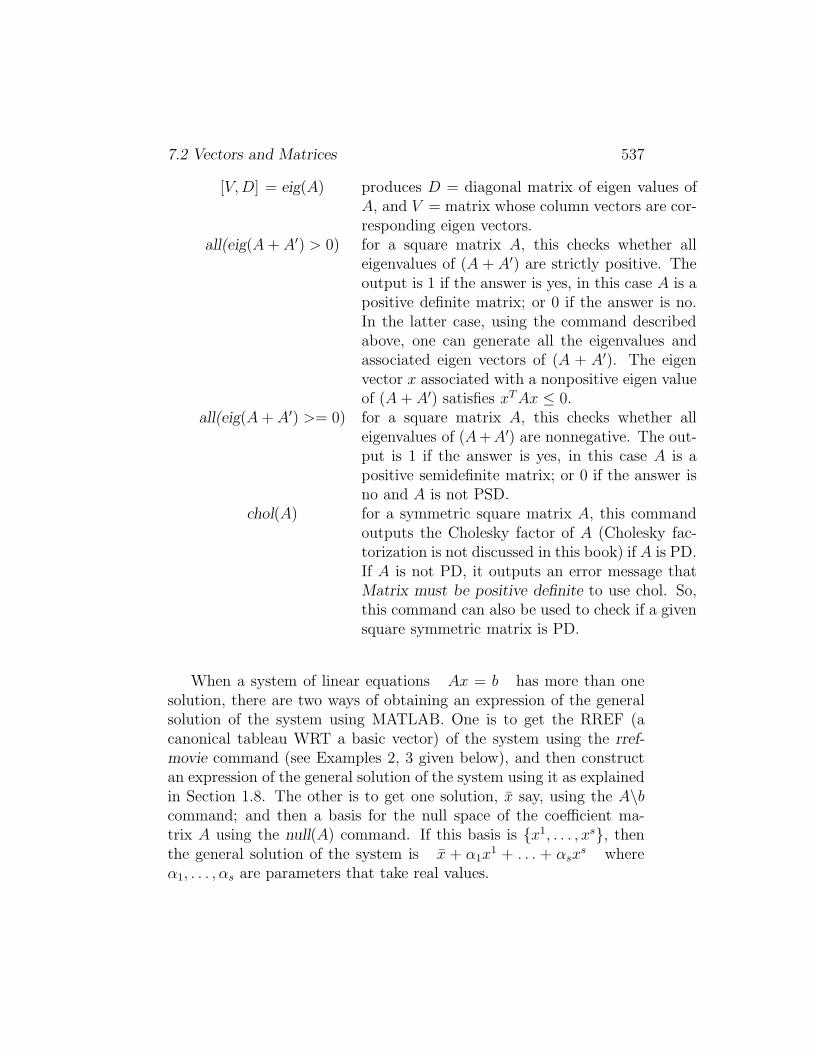
[V, D] = eig(A) produces D = diagonal matrix of eigen values ofA, and V = matrix whose column vectors are cor-responding eigen vectors.
all(eig(A + A′) > 0) for a square matrix A, this checks whether alleigenvalues of (A + A′) are strictly positive. Theoutput is 1 if the answer is yes, in this case A is apositive definite matrix; or 0 if the answer is no.In the latter case, using the command describedabove, one can generate all the eigenvalues andassociated eigen vectors of (A + A′). The eigenvector x associated with a nonpositive eigen valueof (A + A′) satisfies xT Ax ≤ 0.
all(eig(A + A′) >= 0) for a square matrix A, this checks whether alleigenvalues of (A+A′) are nonnegative. The out-put is 1 if the answer is yes, in this case A is apositive semidefinite matrix; or 0 if the answer isno and A is not PSD.
chol(A) for a symmetric square matrix A, this commandoutputs the Cholesky factor of A (Cholesky fac-torization is not discussed in this book) if A is PD.If A is not PD, it outputs an error message thatMatrix must be positive definite to use chol. So,this command can also be used to check if a givensquare symmetric matrix is PD.
When a system of linear equations Ax = b has more than onesolution, there are two ways of obtaining an expression of the generalsolution of the system using MATLAB. One is to get the RREF (acanonical tableau WRT a basic vector) of the system using the rref-movie command (see Examples 2, 3 given below), and then constructan expression of the general solution of the system using it as explainedin Section 1.8. The other is to get one solution, x̄ say, using the A\bcommand; and then a basis for the null space of the coefficient ma-trix A using the null(A) command. If this basis is {x1, . . . , xs}, thenthe general solution of the system is x̄ + α1x
1 + . . . + αsxs where
α1, . . . , αs are parameters that take real values.
538 Ch. 7. Software Systems
7.3 Illustrative Numerical Examples
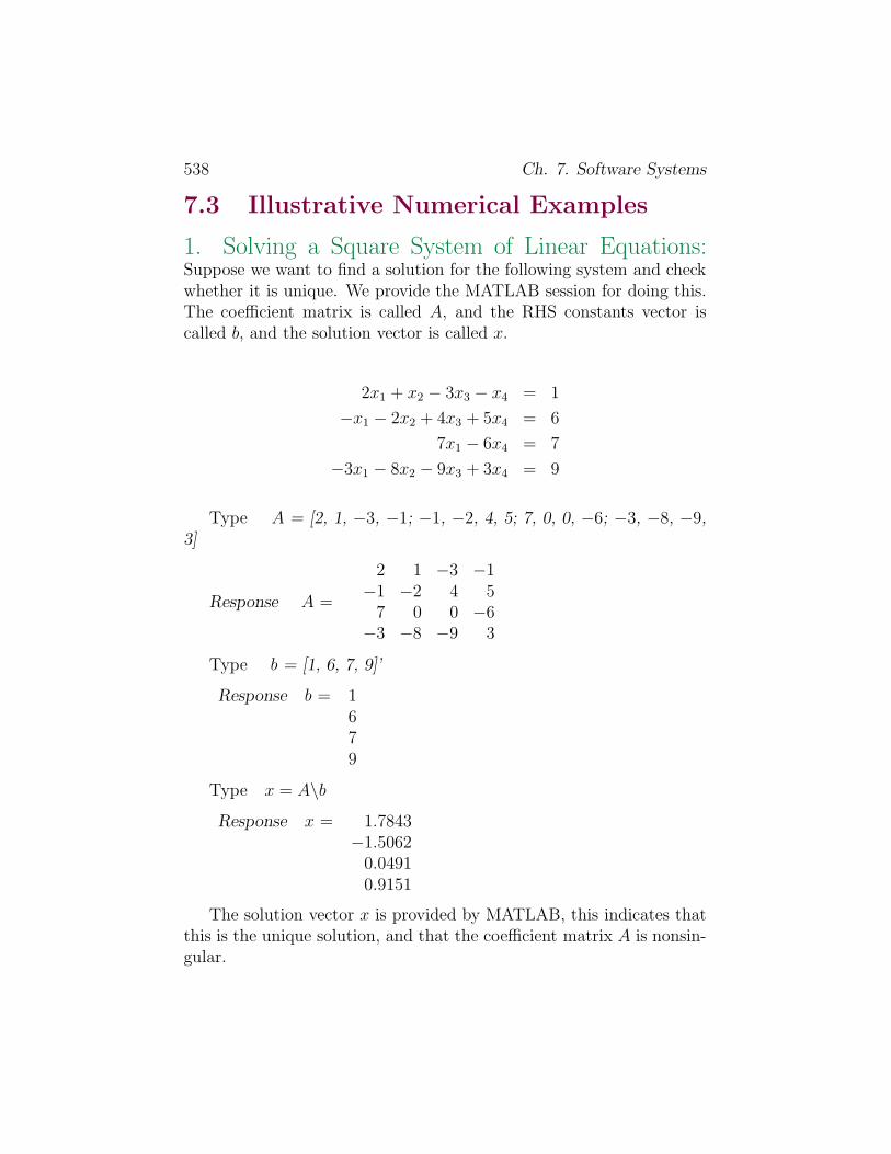
1. Solving a Square System of Linear Equations:Suppose we want to find a solution for the following system and checkwhether it is unique. We provide the MATLAB session for doing this.The coefficient matrix is called A, and the RHS constants vector iscalled b, and the solution vector is called x.
2x1 + x2 − 3x3 − x4 = 1
−x1 − 2x2 + 4x3 + 5x4 = 6
7x1 − 6x4 = 7
−3x1 − 8x2 − 9x3 + 3x4 = 9
Type A = [2, 1, −3, −1; −1, −2, 4, 5; 7, 0, 0, −6; −3, −8, −9,3]
Response A =
2 1 −3 −1−1 −2 4 5
7 0 0 −6−3 −8 −9 3
Type b = [1, 6, 7, 9]’
Response b = 1679
Type x = A\bResponse x = 1.7843
−1.50620.04910.9151
The solution vector x is provided by MATLAB, this indicates thatthis is the unique solution, and that the coefficient matrix A is nonsin-gular.
7.3 Examples 539
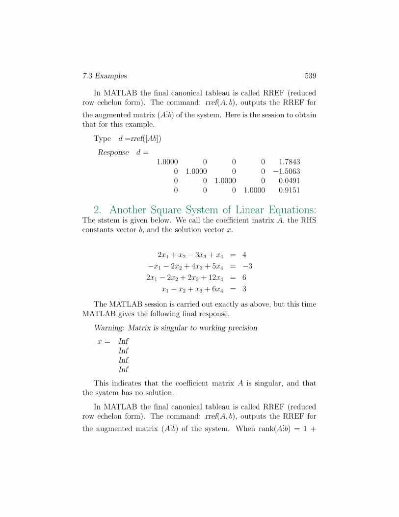
In MATLAB the final canonical tableau is called RREF (reducedrow echelon form). The command: rref(A, b), outputs the RREF for
the augmented matrix (A...b) of the system. Here is the session to obtain
that for this example.
Type d =rref([Ab])
Response d =1.0000 0 0 0 1.7843
0 1.0000 0 0 −1.50630 0 1.0000 0 0.04910 0 0 1.0000 0.9151
2. Another Square System of Linear Equations:The ststem is given below. We call the coefficient matrix A, the RHSconstants vector b, and the solution vector x.
2x1 + x2 − 3x3 + x4 = 4
−x1 − 2x2 + 4x3 + 5x4 = −3
2x1 − 2x2 + 2x3 + 12x4 = 6
x1 − x2 + x3 + 6x4 = 3
The MATLAB session is carried out exactly as above, but this timeMATLAB gives the following final response.
Warning: Matrix is singular to working precision
x = InfInfInfInf
This indicates that the coefficient matrix A is singular, and thatthe syatem has no solution.
In MATLAB the final canonical tableau is called RREF (reducedrow echelon form). The command: rref(A, b), outputs the RREF for
the augmented matrix (A...b) of the system. When rank(A
...b) = 1 +
540 Ch. 7. Software Systems
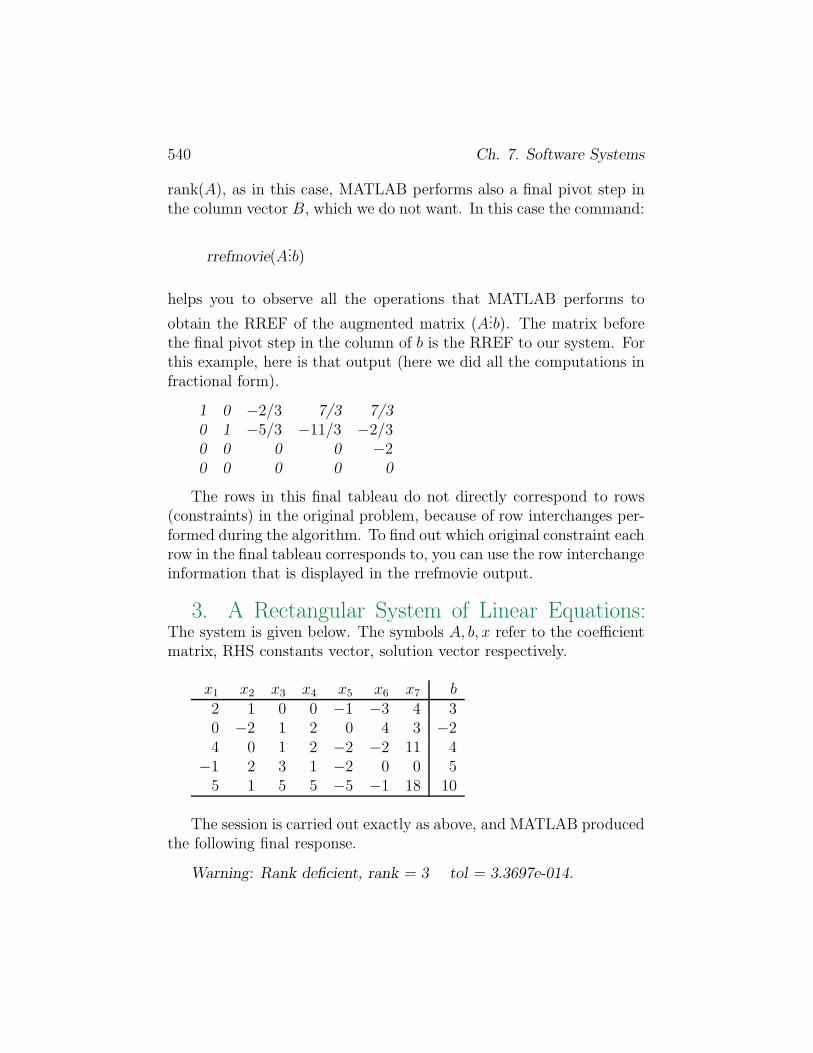
rank(A), as in this case, MATLAB performs also a final pivot step inthe column vector B, which we do not want. In this case the command:
rrefmovie(A...b)
helps you to observe all the operations that MATLAB performs to
obtain the RREF of the augmented matrix (A...b). The matrix before
the final pivot step in the column of b is the RREF to our system. Forthis example, here is that output (here we did all the computations infractional form).
1 0 −2/3 7/3 7/30 1 −5/3 −11/3 −2/30 0 0 0 −20 0 0 0 0
The rows in this final tableau do not directly correspond to rows(constraints) in the original problem, because of row interchanges per-formed during the algorithm. To find out which original constraint eachrow in the final tableau corresponds to, you can use the row interchangeinformation that is displayed in the rrefmovie output.
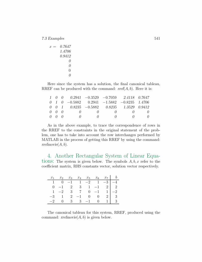
3. A Rectangular System of Linear Equations:The system is given below. The symbols A, b, x refer to the coefficientmatrix, RHS constants vector, solution vector respectively.
x1 x2 x3 x4 x5 x6 x7 b2 1 0 0 −1 −3 4 30 −2 1 2 0 4 3 −24 0 1 2 −2 −2 11 4
−1 2 3 1 −2 0 0 55 1 5 5 −5 −1 18 10
The session is carried out exactly as above, and MATLAB producedthe following final response.
Warning: Rank deficient, rank = 3 tol = 3.3697e-014.
7.3 Examples 541
x = 0.76471.47060.9412
0000
Here since the system has a solution, the final canonical tableau,RREF can be produced with the command: rref(A, b). Here it is:
1 0 0 0.2941 −0.3529 −0.7059 2.4118 0.76470 1 0 −0.5882 0.2941 −1.5882 −0.8235 1.47060 0 1 0.8235 −0.5882 0.8235 1.3529 0.94120 0 0 0 0 0 0 00 0 0 0 0 0 0 0
As in the above example, to trace the correspondence of rows inthe RREF to the constraints in the original statement of the prob-lem, one has to take into account the row interchanges performed byMATLAB in the process of getting this RREF by using the command:rrefmovie(A, b).
4. Another Rectangular System of Linear Equa-tions: The system is given below. The symbols A, b, x refer to thecoefficient matrix, RHS constants vector, solution vector respectively.
x1 x2 x3 x4 x5 x6 x7 b1 0 −1 1 −2 1 −3 −40 −1 2 3 1 −1 2 21 −2 3 7 0 −1 1 −2
−3 1 2 −1 0 0 2 3−2 0 3 3 −1 0 1 3
The canonical tableau for this system, RREF, produced using thecommand: rrefmovie(A, b) is given below.
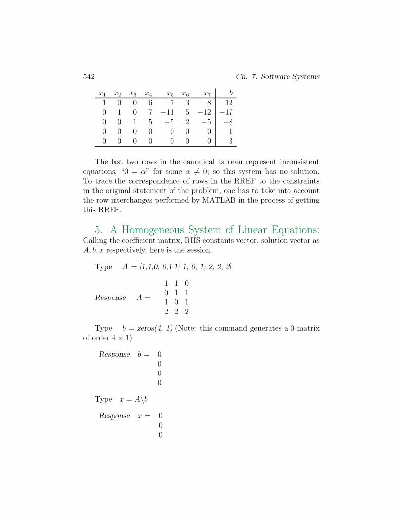
542 Ch. 7. Software Systems
x1 x2 x3 x4 x5 x6 x7 b1 0 0 6 −7 3 −8 −120 1 0 7 −11 5 −12 −170 0 1 5 −5 2 −5 −80 0 0 0 0 0 0 10 0 0 0 0 0 0 3
The last two rows in the canonical tableau represent inconsistentequations, “0 = α” for some α �= 0; so this system has no solution.To trace the correspondence of rows in the RREF to the constraintsin the original statement of the problem, one has to take into accountthe row interchanges performed by MATLAB in the process of gettingthis RREF.
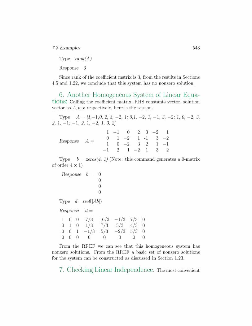
5. A Homogeneous System of Linear Equations:Calling the coefficient matrix, RHS constants vector, solution vector asA, b, x respectively, here is the session.
Type A = [1,1,0; 0,1,1; 1, 0, 1; 2, 2, 2]
Response A =
1 1 00 1 11 0 12 2 2
Type b = zeros(4, 1) (Note: this command generates a 0-matrixof order 4 × 1)
Response b = 0000
Type x = A\bResponse x = 0
00
7.3 Examples 543
Type rank(A)
Response 3
Since rank of the coefficient mstrix is 3, from the results in Sections4.5 and 1.22, we conclude that this system has no nonzero solution.
6. Another Homogeneous System of Linear Equa-tions: Calling the coefficient matrix, RHS constants vector, solutionvector as A, b, x respectively, here is the session.
Type A = [1,−1,0, 2, 3, −2, 1; 0,1, −2, 1, −1, 3, −2; 1, 0, −2, 3,2, 1, −1; −1, 2, 1, −2, 1, 3, 2]
Response A =
1 −1 0 2 3 −2 10 1 −2 1 -1 3 −21 0 −2 3 2 1 −1
−1 2 1 −2 1 3 2
Type b = zeros(4, 1) (Note: this command generates a 0-matrixof order 4 × 1)
Response b = 0000
Type d =rref([Ab])
Response d =
1 0 0 7/3 16/3 −1/3 7/3 00 1 0 1/3 7/3 5/3 4/3 00 0 1 −1/3 5/3 −2/3 5/3 00 0 0 0 0 0 0 0
From the RREF we can see that this homogeneous system hasnonzero solutions. From the RREF a basic set of nonzero solutionsfor the system can be constructed as discussed in Section 1.23.
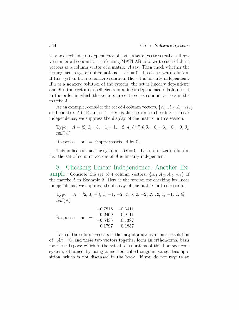
7. Checking Linear Independence: The most convenient
544 Ch. 7. Software Systems
way to check linear independence of a given set of vectors (either all rowvectors or all column vectors) using MATLAB is to write each of thesevectors as a column vector of a matrix, A say. Then check whether thehomogeneous system of equations Ax = 0 has a nonzero solution.If this system has no nonzero solution, the set is linearly independent.If x̄ is a nonzero solution of the system, the set is linearly dependent;and x̄ is the vector of coefficients in a linear dependence relation for itin the order in which the vectors are entered as column vectors in thematrix A.
As an example, consider the set of 4 column vectors, {A.1.A.2, A.3, A.4}of the matrix A in Example 1. Here is the session for checking its linearindependence; we suppress the display of the matrix in this session.
Type A = [2, 1, −3, −1; −1, −2, 4, 5; 7, 0,0, −6; −3, −8, −9, 3];
null(A)
Response ans = Empty matrix: 4-by-0.
This indicates that the system Ax = 0 has no nonzero solution,i.e., the set of column vectors of A is linearly independent.
8. Checking Linear Independence, Another Ex-ample: Consider the set of 4 column vectors, {A. 1.A. 2, A. 3, A. 4 } ofthe matrix A in Example 2. Here is the session for checking its linearindependence; we suppress the display of the matrix in this session.
Type A = [2, 1, −3, 1; −1, −2, 4, 5; 2, −2, 2, 12; 1, −1, 1, 6];
null(A)
Response ans =
−0.7818 −0.3411−0.2469 0.9111−0.5436 0.1382
0.1797 0.1857
Each of the column vectors in the output above is a nonzero solutionof Ax = 0 and these two vectors together form an orthonormal basisfor the subspace which is the set of all solutions of this homogeneoussystem, obtained by using a method called singular value decompo-sition, which is not discussed in the book. If you do not require an
7.3 Examples 545
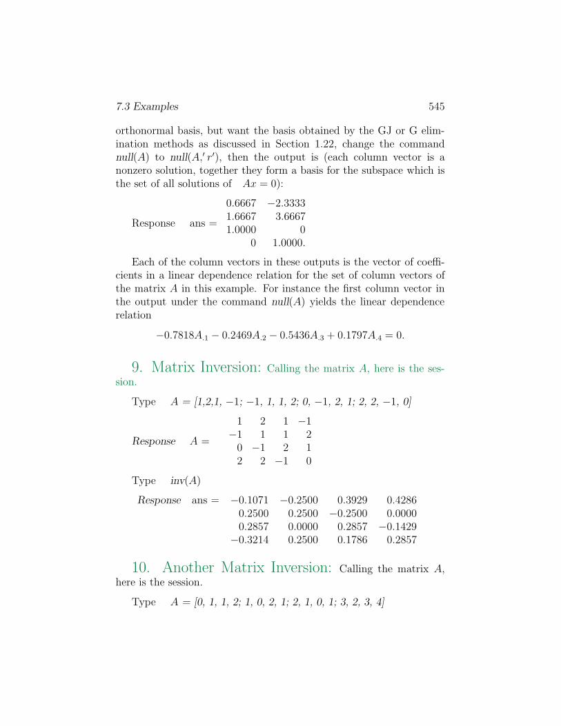
orthonormal basis, but want the basis obtained by the GJ or G elim-ination methods as discussed in Section 1.22, change the commandnull(A) to null(A,′ r′), then the output is (each column vector is anonzero solution, together they form a basis for the subspace which isthe set of all solutions of Ax = 0):
Response ans =
0.6667 −2.33331.6667 3.66671.0000 0
0 1.0000.
Each of the column vectors in these outputs is the vector of coeffi-cients in a linear dependence relation for the set of column vectors ofthe matrix A in this example. For instance the first column vector inthe output under the command null(A) yields the linear dependencerelation
−0.7818A. 1 − 0.2469A. 2 − 0.5436A. 3 + 0.1797A. 4 = 0.
9. Matrix Inversion: Calling the matrix A, here is the ses-sion.
Type A = [1,2,1, −1; −1, 1, 1, 2; 0, −1, 2, 1; 2, 2, −1, 0]
Response A =
1 2 1 −1−1 1 1 2
0 −1 2 12 2 −1 0
Type inv(A)
Response ans = −0.1071 −0.2500 0.3929 0.42860.2500 0.2500 −0.2500 0.00000.2857 0.0000 0.2857 −0.1429
−0.3214 0.2500 0.1786 0.2857
10. Another Matrix Inversion: Calling the matrix A,here is the session.
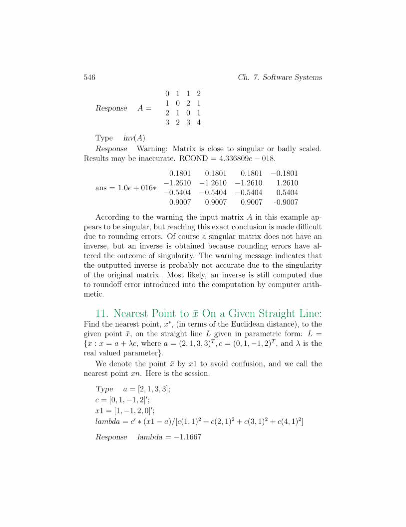
Type A = [0, 1, 1, 2; 1, 0, 2, 1; 2, 1, 0, 1; 3, 2, 3, 4]
546 Ch. 7. Software Systems
Response A =
0 1 1 21 0 2 12 1 0 13 2 3 4
Type inv(A)
Response Warning: Matrix is close to singular or badly scaled.Results may be inaccurate. RCOND = 4.336809e − 018.
ans = 1.0e + 016∗0.1801 0.1801 0.1801 −0.1801
−1.2610 −1.2610 −1.2610 1.2610−0.5404 −0.5404 −0.5404 0.5404
0.9007 0.9007 0.9007 -0.9007
According to the warning the input matrix A in this example ap-pears to be singular, but reaching this exact conclusion is made difficultdue to rounding errors. Of course a singular matrix does not have aninverse, but an inverse is obtained because rounding errors have al-tered the outcome of singularity. The warning message indicates thatthe outputted inverse is probably not accurate due to the singularityof the original matrix. Most likely, an inverse is still computed dueto roundoff error introduced into the computation by computer arith-metic.
11. Nearest Point to x̄ On a Given Straight Line:Find the nearest point, x∗, (in terms of the Euclidean distance), to thegiven point x̄, on the straight line L given in parametric form: L ={x : x = a + λc, where a = (2, 1, 3, 3)T , c = (0, 1,−1, 2)T , and λ is thereal valued parameter}.
We denote the point x̄ by x1 to avoid confusion, and we call thenearest point xn. Here is the session.
Type a = [2, 1, 3, 3];
c = [0, 1,−1, 2]′;x1 = [1,−1, 2, 0]′;lambda = c′ ∗ (x1 − a)/[c(1, 1)2 + c(2, 1)2 + c(3, 1)2 + c(4, 1)2]
Response lambda = −1.1667
7.3 Examples 547
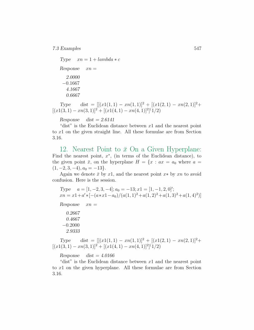
Type xn = 1 + lambda ∗ c
Response xn =
2.0000−0.1667
4.16670.6667
Type dist = [[(x1(1, 1) − xn(1, 1)]2 + [(x1(2, 1) − xn(2, 1)]2+[(x1(3, 1) − xn(3, 1)]2 + [(x1(4, 1) − xn(4, 1)]2](1/2)
Response dist = 2.6141“dist” is the Euclidean distance between x1 and the nearest point
to x1 on the given straight line. All these formulae are from Section3.16.
12. Nearest Point to x̄ On a Given Hyperplane:Find the nearest point, x∗, (in terms of the Euclidean distance), tothe given point x̄, on the hyperplane H = {x : ax = a0 where a =(1,−2, 3,−4), a0 = −13}.
Again we denote x̄ by x1, and the nearest point x∗ by xn to avoidconfusion. Here is the session.
Type a = [1,−2, 3,−4]; a0 = −13; x1 = [1,−1, 2, 0]′;xn = x1+a′∗ [−(a∗x1−a0)/(a(1, 1)2+a(1, 2)2+a(1, 3)2+a(1, 4)2)]
Response xn =
0.26670.4667
−0.20002.9333
Type dist = [[(x1(1, 1) − xn(1, 1)]2 + [(x1(2, 1) − xn(2, 1)]2+[(x1(3, 1) − xn(3, 1)]2 + [(x1(4, 1) − xn(4, 1)]2](1/2)
Response dist = 4.0166“dist” is the Euclidean distance between x1 and the nearest point
to x1 on the given hyperplane. All these formulae are from Section3.16.
548 Ch. 7. Software Systems
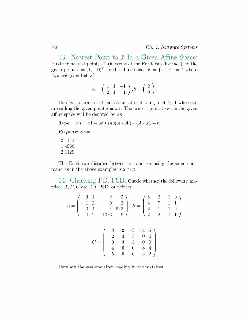
13. Nearest Point to x̄ In a Given Affine Space:Find the nearest point, x∗, (in terms of the Euclidean distance), to thegiven point x̄ = (1, 1, 0)T , in the affine space F = {x : Ax = b whereA, b are given below}.
A =
(1 1 −12 1 1
), b =
(29
).
Here is the portion of the session after reading in A, b, x1 where weare calling the given point x̄ as x1. The nearest point to x1 in the givenaffine space will be denoted by xn.
Type xn = x1 − A′ ∗ inv(A ∗ A′) ∗ (A ∗ x1 − b)
Response xn =
2.71431.42862.1429
The Euclidean distance between x1 and xn using the same com-mand as in the above examples is 2.7775.
14. Checking PD, PSD: Check whether the following ma-trices A, B, C are PD, PSD, or neither.
A =
3 1 2 2−1 2 0 2
0 4 4 5/30 2 −13/3 6
, B =
8 2 1 04 7 −1 12 1 1 22 −2 1 1
C =
0 −2 −3 −4 52 3 3 0 03 3 3 0 04 0 0 8 4
−5 0 0 4 2
Here are the sessions after reading in the matrices.
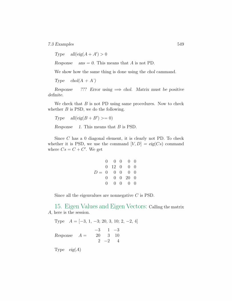
7.3 Examples 549
Type all(eig(A + A′) > 0
Response ans = 0. This means that A is not PD.
We show how the same thing is done using the chol cammand.
Type chol(A + A’)
Response ??? Error using =⇒ chol. Matrix must be positivedefinite.
We check that B is not PD using same procedures. Now to checkwhether B is PSD, we do the following.
Type all(eig(B + B′) >= 0)
Response 1. This means that B is PSD.
Since C has a 0 diagonal element, it is clearly not PD. To checkwhether it is PSD, we use the command [V, D] = eig(Cs) commandwhere Cs = C + C ′. We get
D =
0 0 0 0 00 12 0 0 00 0 0 0 00 0 0 20 00 0 0 0 0
Since all the eigenvalues are nonnegative C is PSD.
15. Eigen Values and Eigen Vectors: Calling the matrixA, here is the session.
Type A = [−3, 1, −3; 20, 3, 10; 2, −2, 4]
Response A =−3 1 −320 3 102 −2 4
Type eig(A)
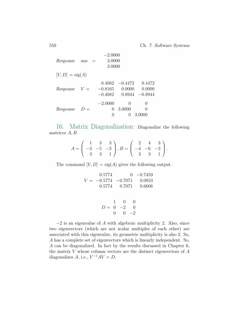
550 Ch. 7. Software Systems
Response ans =−2.0000
3.00003.0000
[V, D] = eig(A)
Response V =0.4082 −0.4472 0.4472
−0.8165 0.0000 0.0000−0.4082 0.8944 −0.8944
Response D =−2.0000 0 0
0 3.0000 00 0 3.0000
16. Matrix Diagonalization: Diagonalize the followingmatrices A, B.
A =
1 3 3
−3 −5 −33 3 1
, B =
2 4 3
−4 −6 −33 3 1
.
The command [V, D] = eig(A) gives the following output.
V =0.5774 0 −0.7459
−0.5774 −0.7071 0.08530.5774 0.7071 0.6606
D =1 0 00 −2 00 0 −2
−2 is an eigenvalue of A with algebraic multiplicity 2. Also, sincetwo eigenvectors (which are not scalar multiples of each other) areassociated with this eigenvalue, its geometric multiplicity is also 2. So,A has a complete set of eigenvectors which is linearly independent. So,A can be diagonalized. In fact by the results discussed in Chapter 6,the matrix V whose column vectors are the distinct eigenvectors of Adiagonalizes A, i.e., V −1AV = D.
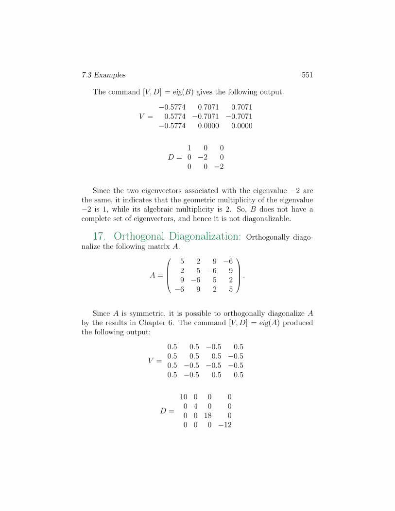
7.3 Examples 551
The command [V, D] = eig(B) gives the following output.
V =−0.5774 0.7071 0.7071
0.5774 −0.7071 −0.7071−0.5774 0.0000 0.0000
D =1 0 00 −2 00 0 −2
Since the two eigenvectors associated with the eigenvalue −2 arethe same, it indicates that the geometric multiplicity of the eigenvalue−2 is 1, while its algebraic multiplicity is 2. So, B does not have acomplete set of eigenvectors, and hence it is not diagonalizable.
17. Orthogonal Diagonalization: Orthogonally diago-nalize the following matrix A.
A =
5 2 9 −62 5 −6 99 −6 5 2
−6 9 2 5
.
Since A is symmetric, it is possible to orthogonally diagonalize Aby the results in Chapter 6. The command [V, D] = eig(A) producedthe following output:
V =
0.5 0.5 −0.5 0.50.5 0.5 0.5 −0.50.5 −0.5 −0.5 −0.50.5 −0.5 0.5 0.5
D =
10 0 0 00 4 0 00 0 18 00 0 0 −12
552 Ch. 7. Software Systems
By the results in Chapter 6, the matrix V whose column vectorsform a complete set of eigenvectors for A orthogonally diagonalize A,i.e., V T AV = D.
7.4 References
References on MATLAB
[7.1] M. Golubitsky and M. Dellnitz, Linear Algebra and DifferentialEquations Using MATLAB, Brooks/Cole Publishing Co., NY, 1999.[7.2] E. B. Magrab and others, An Engineer’s Guide to MATLAB,Prentice Hall, Upper Saddle River, NJ, 2000.7.3] C. F. Van Loan, Introduction to Scientific Computing, MATLABCurriculum Series, Prentice Hall, Upper Saddle River, NJ, 1997.[7.4] The Student Edition of MATLAB, Users Guide, The MathWorksInc., Natick, MA.
References on Other Software Systems
[7.5] B. W. Char, et. al. First Leaves: A Tutorial Introduction toMaple V, Springer Verlag, NY, 1992.[7.6] J. H. Davenport, Computer Algebra: Systems and Algorithms forAlgebraic Computation, Academic Press, San diago, 1993.[7.7] D. Eugene, Schaum’s Outline of Theory and Problems of Mathe-matica, McGraw-Hill, NY, 2001.[7.8] M. B. Monagan, et. al., Maple V Programming Guide, Springer,NY, 1998.[7.9] Microsoft Corp., Microsoft Excel User’s Guide, Version 5.0, Red-mond, WA, 1993.[7.10] S. Wolfram, The Mathematica Book, 3rd ed., Wolfram Media,Cambridge University Press, 1996.