Embed Size (px)
Citation preview
Toric Schemes
Dissertation
zur
Erlangung der naturwissenschaftlichen Doktorwurde
(Dr. sc. nat.)
vorgelegt der
Mathematisch-naturwissenschaftlichen Fakultat
der
Universitat Zurich
von
Fred Rohrer
von
Buchs SG
Promotionskomitee
Prof. Dr. Markus Brodmann (Vorsitz)
Prof. Dr. Andrew Kresch
Prof. Dr. Christian Okonek
Zurich, 2010
2010 Mathematics Subject Classification. Primary 14M25;
Secondary 13A02, 13D45, 16W50, 14A15, 52A07, 52A21, 52B99
Wir mussen wissen,
wir werden wissen.
D. Hilbert
To Barbara
Contents
Preface ix
Introduction xi
Notations and conventions 1
Chapter I. Algebras of monoids 5
1. Spectra of bigebras of monoids 6
1.1. Monoids, comonoids, and monomodules 6
1.2. Generalities on monoids 9
1.3. Algebras and bigebras of monoids 12
1.4. Spectra of algebras and bigebras of monoids 19
2. Geometric properties of algebras of monoids 25
2.1. Separatedness and finiteness conditions 25
2.2. Faithful flatness 26
2.3. Reducedness, irreducibility, and integrality 27
2.4. Connectedness 30
2.5. Normality 31
2.6. Chain conditions and dimension theory 31
Chapter II. Cones and fans 35
1. Polycones 36
1.1. Structures on real vector spaces of finite dimension 36
1.2. Convex and conic sets 43
1.3. Faces of conic sets 50
1.4. Polycones 55
1.5. Direct sums and decompositions of polycones 64
2. Fans 69
2.1. Semifans 69
2.2. Fans 72
2.3. Topological properties of fans 75
2.4. Subdivisions 82
3. Completions of fans 86
3.1. Relatively simplicial extensions 87
3.2. Separable extensions 89
3.3. Packings and strong completions 91
3.4. Construction of complete fans 93
3.5. Adjustments of extensions 96
vi Contents
3.6. Pullbacks of extensions 99
3.7. Existence of packings and completions 108
4. The combinatorics of a fan 111
4.1. The Picard group of a fan 111
4.2. The standard diagram of a fan 115
4.3. Projective systems of monoids defined by fans 118
Chapter III. Graduations 121
1. Quasigraduations and graduations 122
1.1. Quasigraduations 122
1.2. Graded rings and modules 125
1.3. Coarsening and refinement 126
1.4. Extension and restriction 129
2. Categories of graded modules 133
2.1. Abelianity of categories of graded modules 133
2.2. Free graded modules 135
2.3. Hom functors 136
2.4. Projective and injective graded modules 140
2.5. Graded rings and modules of fractions 143
3. Further properties of graded rings and modules 147
3.1. Strong graduations 147
3.2. Saturation 148
3.3. Noetherianity 149
3.4. Hilbert’s Basissatz and the Artin-Rees Lemma 150
3.5. Projective systems of ideals 154
3.6. Torsion functors 155
4. Cohomology of graded modules 158
4.1. Complexes and cocomplexes 158
4.2. Resolutions 159
4.3. Extension functors 160
4.4. Local cohomology and higher ideal transformation 163
4.5. Cech cohomology 171
Chapter IV. Toric Schemes 177
1. Toric schemes 178
1.1. Toric schemes 178
1.2. Basic properties of toric schemes 182
1.3. Projections of fans and properness of toric schemes 183
2. Cox schemes 190
2.1. Cox rings 190
2.2. Cox schemes 193
2.3. Cox schemes and toric schemes 196
3. Sheaves of modules on toric schemes 198
3.1. Sheaves associated with graded modules 198
3.2. The first total functor of sections 204
Contents vii
3.3. On surjectivity of SΣ 208
3.4. On injectivity of SΣ 212
4. Cohomology of toric schemes 215
4.1. The second total functor of sections 215
4.2. The toric Serre-Grothendieck correspondence 218
Logical Bibliography 225
Additional Bibliography 227
Index of Notations 229
Index of Terminology 233

Preface
This thesis presents foundations for a theory of toric schemes, generalis-
ing the theory of toric varieties. No knowledge about the latter is required
from – but of course may be helpful to – the reader. The prerequisites
are very moderate throughout. Only some basics in the following fields are
assumed:
· foundations, including the language of categories ([E], [7]);
· commutative and homological algebra ([A], [AC], [6]);
· topology, including topological vector spaces ([TG], [EVT]);
· algebraic geometry ([EGA, I]).
To be more precise, the references from which something is used to build up
the theory are given in a Logical Bibliography. Besides this an Additional
Bibliography is provided, giving references that are cited only in motivating,
explaining or historical comments.
Some conventions about notation and terminology are given at the be-
ginning, and moreover indices of notation and of terminology are provided
at the end. At the beginning of each chapter or section, general hypotheses
and abbreviations kept in force during this part of text are given in italics.
There are very few logical dependencies between the first three chap-
ters, whereas the fourth chapter makes heavy use of most that precedes it.
Paragraphs in small print are not logically necessary for what follows them
(except further paragraphs in small print) and consist mainly of examples
and counterexamples.
I am very grateful to Prof. Markus Brodmann for his support during
the past years, including hours of interesting and motivating discussions; I
highly appreciate the freedom he gave me of doing what I liked most. I also
thank Prof. Ngo Vie.t Trung for refereeing the thesis, Prof. Rodney Y. Sharp
for his interest in my work and his support, and my colleagues at the In-
stitute of Mathematics of the University of Zurich during the past years,
especially Stefan Fumasoli for teaching me a lot of algebraic geometry, Felix
Fontein for answering a question with a custom-made LATEX-package, and
Urs Kollbrunner and Dominic Schuhmacher for a lot of fun at the Cafete-
ria. A very special thank-you goes to my Haggy for constant encouraging
support.

Introduction
L’objet de la Geometrie algebrique [...]
est donc l’etude des schemas.A. Grothendieck
The theory of toric varieties, developed since the 1970’s and still bring-
ing forth a lot of works today, obviously deals with toric varieties. Strangely
enough, to my knowledge there was never published a serious attempt to
develop this theory in the framework of schemes, that is, a theory of toric
schemes. The lecture notes by Kempf, Knudsen, Mumford and Saint-Donat
on toroidal embeddings ([16]), which might be considered as the first appear-
ance of toric varieties, end with a small step in this direction by swapping the
algebraically closed base field for a discrete valuation ring. In later sources,
most authors went back to algebraically closed fields or even complex num-
bers (and of course also made use of the additional structures available in the
latter case; see for example Oda’s book [20]). But with the well-developed
theory of schemes at hand – being moreover easier and more natural than
the theory of varieties – there is no reason to do so. On the contrary, from a
conceptual point of view it seems desirable to have a theory of toric schemes,
and the goal of this thesis is to elaborate – or at least lay the foundations
for – such a theory.
Besides this general reason to consider toric schemes there are some
more specific ones, mostly the treatment of functorial questions about toric
varieties. It was a question of this type, namely representability of Hilbert
functors, that was at the origin of this work. The definition of Hilbert
functor of a toric variety X (see [14]) obviously leads to arbitrary (or at
least affine) base changes of X and hence to “toric varieties over arbitrary
base rings”, that is, toric schemes. Without a theory of toric schemes every
approach to the question of representability of this functor in the spirit of
[17] is bound to fail, for known proofs of results about toric varieties often
do not just carry over to toric schemes, although the results themselves may
do. One reason for this is that a lot of proofs for toric varieties are based
on Weil divisor techniques while Weil divisors are not necessarily defined
on toric schemes. This implies in particular that a theory of toric schemes
will provide new proofs for old results about toric varieties, avoiding Weil
divisors and hence being probably easier (or at least more combinatorial).
xii Introduction
Throughout this work I tried to attack all the problems in great general-
ity and moreover emphasise functoriality of the involved notions. Not only
may these principles be helpful in proving theorems, but I am convinced
that in addition they help in understanding what is going on. Functoriality
may explain more precisely how some term depends on other terms, and
generality may reveal whose guilt it is that some statement is true or not.
These principles and the wish for a rigorous exposition without too many
prerequisites – also as a basis for future work – are the reason why some
parts of the following are surely well-known, known, or at least partially
known in one form or the other.
I will now give a chapterwise brief summary, and inform the reader that
there will be more detailed information at the beginning of each chapter.
In Chapter I, the algebraic foundations are treated, that is, functors of
algebras and bigebras of monoids. Moreover, we consider schemes glued from
spectra of bigebras of monoids defined by projective systems of monoids, and
investigate their geometry. Later on, toric schemes are defined as a special
case of this construction.
Chapter II contains the combinatorial ingredients, that is, cones and
fans. Since I know of no satisfying treatment of this we develop it from
scratch in an abstract way, avoiding coordinates and using purely topological
arguments if possible. As a highlight of the whole thesis I would like to
mention the Completion Theorem; it shows that every (simplicial) fan has a
(simplicial) completion, that is, it can be extended to a (simplicial) fan that
covers the ambient space.
Some more algebraic work is done in Chapter III on graduations. We
consider rings and modules graded by arbitrary groups and their behaviour
under functors like coarsening or restriction of degrees. Furthermore, we
develop some homological algebra, including local cohomology, of arbitrarily
graded modules.
Finally, in Chapter IV everything is put together. First, a fan Σ gives
rise to a projective system of monoids, and the techniques from Chapter
I yield for every ring R the toric scheme XΣ(R). Second, based on Cox’s
influental article [10] we associate with every fan Σ and every ring R the
so-called Cox ring and the so-called Cox scheme YΣ(R), together with a
canonical morphism YΣ(R)→ XΣ(R). This morphism is an isomorphism if
and only if Σ is not contained in a hyperplane and hence allows to study Cox
schemes instead of toric schemes. Third, using our work on graduations from
Chapter III we generalise further results from [10] to describe quasicoherent
sheaves of modules on Cox schemes in terms of graded modules over the
corresponding Cox ring. More precisely, we show how a graded module
over the Cox ring gives rise to a quasicoherent sheaf of modules on the
Cox scheme YΣ(R), that every quasicoherent sheaf of modules on YΣ(R)
arises like this, and – if Σ is simplicial – that this correspondence induces a
Introduction xiii
bijection between graded ideals of a certain restriction of the Cox ring that
are saturated with respect to the so-called irrelevant ideal, and quasicoherent
ideals of the structure sheaf on YΣ(R). Finally, a toric version of the Serre-
Grothendieck correspondence gives a relation between sheaf cohomology on
Cox schemes and local cohomology over the corresponding Cox ring.

Notations and conventions
(1) In general, we use the terminology of Bourbaki’s Elements de mathe-
matique and Grothendieck’s Elements de geometrie algebrique, and unex-
plained terminology or notation is meant to refer to these treatises. Further
remarks and reminders on terminology will be given in footnotes, and we
provide indices of notations and of terminology.
(2) As a logical framework we use Bourbaki’s Theory of Sets ([E]), includ-
ing the axioms UA and UB concerning universes ([1, I.0; I.11]). Some of the
following is tacitly meant relatively to a universe U containing an infinite
set and chosen once and for all. The objects considered are often tacitly
supposed to be elements of U . A few remarks on set theoretical questions
will be given in small print and indicated by “Concerning set theory, ...”.
(3) We define categories accordingly to [7]. The categories considered are
often tacitly supposed to be U-categories or even U-small categories. If C is
a category, then we denote by C its dual category and by Ob(C) the set of
objects of C, and for objects A and B of C we denote by HomC(A,B) the set
of morphism in C from A to B and by IdA the identity morphism of A. If C
is a category and A is an object of C, then we denote by C/A the category
of objects over A in C, and by C/A the category of objects under A in C. If
C is an Abelian category, then we denote by Co(C) and CCo(C) respectively
the categories of complexes and cocomplexes in C (see III.4.1.1).
By a functor we always mean a covariant functor. If C and D are cate-
gories, then we denote by Hom(C,D) the category of functors from C to D.
For a strictly positive number k, by a k-functor (or bifunctor in case k = 2)
we mean a functor whose source is a product of k categories (although in
fact every functor has this property). Further notions involving the variance
of the arguments of k-functors like “contra-covariant bifunctor” are hoped
to be self-explaining.
In diagrams we use arrows of the form and to denote mono- and
epimorphisms, and sometimes we denote canonical injections of subobjects
by arrows of the form →.
(4) We denote by Ens the category of sets that are elements of the universe
U . We denote by N0, N, Z and Q the sets of natural numbers, of strictly
positive natural numbers, of integers, and of rational numbers.
2 Notations and conventions
(5) We denote by Ord the category of ordered sets that are elements of the
universe U , with morphisms the increasing maps. If (E,≤) is a preordered
set and x ∈ E, then we set E≥x := y ∈ E | y ≥ x, and we define
analogously the sets E≤x, E>x and E<x.
(6) By a monoid or a group we always mean a commutative monoid or
group, and we denote by Mon and Ab the categories of monoid and groups
that are elements of the universe U . Mostly, monoids will be written addi-
tively. If M is a monoid, then we call a set furnished with an M -action an
M -monomodule, and if M is an element of U , then we denote by Mod(M)
the category of M -monomodules that are elements of U , with morphisms
the homomorphisms of sets with M -actions.
(7) By a ring we always mean a commutative ring, and we denote by
Ann the category of rings that are elements of the universe U . If R is a
ring, then by an R-algebra we always mean a commutative, unital, asso-
ciative R-algebra, and by an R-bigebra we always mean a commutative,
cocommutative, unital, counital, associative, coassociative R-bigebra. If R
is an element of U , then we denote by Alg(R) and Big(R) the categories
of R-algebras and R-bigebras that are elements of U , with morphisms the
unital homomorphisms of R-algebras and R-bigebras. If R′ is an R-algebra,
then by its multiplication and unit we mean the morphisms of R-modules
R′ ⊗R R′ → R′ and R → R′ respectively defining the structure on R′, and
similarly for the comultiplication and counit of an R-bigebra.
(8) Let R be a ring. For S ⊆ R we denote by S−1R the ring of fractions
of R with denominators in S and by ηS(R) : R→ S−1R or, if no confusion
can arise, by ηS the canonical morphism of rings. In case S = f for some
f ∈ R, or S = R \ p for some p ∈ Spec(R), we write Rf and ηf , or Rp and
ηp, instead of S−1R and ηS (see also III.2.5.4).
We denote by Nil(R) and Idem(R) respectively the sets of nilpotent and
idempotent elements of R, and by Min(R) the set of minimal prime ideals
of R.
(9) If R is a ring that is an element of the universe U , then we denote by
Mod(R) the category of R-modules that are elements of U , with morphisms
the homomorphisms of R-modules. If R is a ring and E and F are R-
modules, then we write HomR(E,F ) instead of HomMod(R)(E,F ). For an
R-module E and a subset X ⊆ E we denote by 〈X〉R, and if no confusion can
arise by 〈X〉, the sub-R-module of E generated by X. If R is a topological
ring that is an element of U , then we denote by TopMod(R) the category of
topological R-modules that are elements of U .
Concerning homological algebra we use the terminology of δ-functors
from [6].
Notations and conventions 3
(10) We denote by Sch the category of schemes that are elements of the
universe U . If C is a category and S is a scheme, then by abuse of language
a morphism u : F → G of functors or of contravariant functors from C to
Sch/S is called an immersion, an open immersion, or a closed immersion,
respectively, if u(C) is an immersion, an open immersion, or a closed im-
mersion for every C ∈ Ob(C). Furthermore, by abuse of language a family
(ui : Fi → G)i∈I of open immersions of functors or of contravariant functors
from C to Sch/S is called an (affine) open covering of G if (ui(C)(Fi(C)))i∈Iis an (affine) open covering of G(C) for every C ∈ Ob(C).
If R is a ring and no confusion can arise, we sometimes write R instead
of Spec(R).
(11) If X is a topological space and A ⊆ X, then we denote by inX(A),
clX(A) and frX(A) respectively the interior, the closure and the frontier of
A. If no confusion can arise, we write just in(A), cl(A) and fr(A) for these
sets.

CHAPTER I
Algebras of monoids
This chapter introduces and investigates the algebraic foundations for
the theory of toric schemes: the functors of algebras and bigebras of monoids.
In Section 1 we start with categorical and elementary generalities on
monoids. Then, we define the functors of algebras and bigebras of monoids,
that is, a bifunctor
•[ ] : Ann×Mon→ Ann,
mapping a ring R and a monoid M onto an R-bigebra R[M ]. By composi-
tion with the contravariant functor Spec : Ann→ Sch we get affine schemes
(with some additional structure) of the form Spec(R[M ]) for a ring R and a
monoid M . If we replace the monoid M by a projective system of monoids
M over a preordered set I, then we can – under the hypothesis that M is
so-called openly immersive and that I is a lower semilattice, – glue the R-
schemes Spec(R[M(i)]) to obtain an R-scheme XM(R) (with some additional
structure), and this construction is still functorial in R. In Chapter IV, toric
schemes will be defined as a special case of this construction. As appropriate
for a scheme-theoretical approach we have emphasised throughout functori-
ality and behaviour under base change of the constructions introduced.
In Section 2 we investigate geometric properties of schemes of the above
form XM(R). We look mainly at the following question:
Given an openly immersive projective system of monoids M over a lower
semilattice, which properties of schemes are respected or reflected by the
functor that maps a ring R onto the R-scheme XM(R)?
This question can often be reduced to the corresponding question about
algebras of monoids, that is:
Given a monoid M , which properties of rings are respected or reflected
by the functor that maps a ring R onto the R-algebra R[M ] of a monoid
M?
Fortunately a lot is known about this question, and we make use of some non-
trivial answers taken from Gilmer’s treatise [5] on Commutative semigroup
rings. As is seen there, some of the properties investigated here, e.g. re-
ducedness, or connectedness, may behave not well in general, but they do
under further hypotheses on the monoids involved. We do not hesitate to
demand these hypotheses as they are fulfilled by the monoids occuring in
the application to toric schemes that we have in mind. So, if the monoid
M is torsionfree, cancellable and finitely generated, then a lot of elementary
6 I. Algebras of monoids
properties are respected and reflected between R and R[M ], and we can
rephrase this roughly by saying that algebras of monoids (and more general,
schemes of the form XM(R)) are as nice (or as ugly) as their base rings.
But one should take this with care, for besides the properties investigated
here there are reasonable properties with a bad behaviour under the func-
tor •[M ]. As an example we may mention Cohen-Macaulayness of R[M ],
depending in general on the characteristic of R as shown by Trung and Hoa
in [22].
The choice of properties considered here is somewhat arbitrary but in-
cludes enough to show that in general there are too much defects to have a
theory of Weil divisors on toric schemes, as mentioned in the Introduction.
1. Spectra of bigebras of monoids
1.1. Monoids, comonoids, and monomodules
Let C be a category.
We start with some general nonsense about monoids and comonoids in
arbitrary categories. Later on, this will be used on one hand to define a
“torus action” on toric schemes, and on the other hand to see that this
structure is canonical (1.4.13, IV.1.1.2).
(1.1.1) We define the category Mon(C) of monoids in C accordingly to
[EGA, 0.1.6]1. Furthermore, we define the category Com(C) of comonoids
in C to be the category Mon(C) of monoids in the dual C of C.
Now, suppose that C has finite coproducts (and in particular an initial
object I). For A ∈ Ob(C) let iA denote the unique morphism I → A, and for
A,B ∈ Ob(C) let σAB denote the canonical isomorphism AqB∼=−→ B qA.
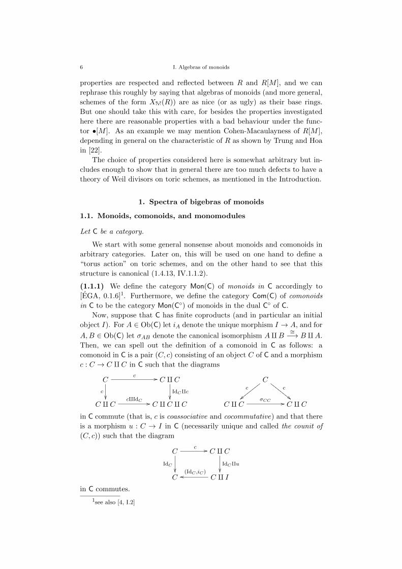
Then, we can spell out the definition of a comonoid in C as follows: a
comonoid in C is a pair (C, c) consisting of an object C of C and a morphism
c : C → C q C in C such that the diagrams
Cc //
c
C q CIdCqc
Cc
||xxxxxxxxc
""FFFFFFFF
C q CcqIdC // C q C q C C q C
σCC // C q Cin C commute (that is, c is coassociative and cocommutative) and that there
is a morphism u : C → I in C (necessarily unique and called the counit of
(C, c)) such that the diagram
Cc //
IdC
C q CIdCqu
C C q I
(IdC ,iC)oo
in C commutes.
1see also [4, I.2]
1. Spectra of bigebras of monoids 7
(1.1.2) Example Let R be a ring. Then, the category Com(Alg(R)) of
comonoids in the category Alg(R) of R-algebras and the category Big(R) of
R-bigebras are canonically isomorphic (see [A, III.11.4]).
(1.1.3) Example Suppose that C has an empty object ∅, that is, an object ∅such that for every A ∈ Ob(C) that is not initial there exists no morphism A→ ∅.Equivalently, ∅ is initial, and every morphism with target ∅ is an isomorphism. In
particular, it holds ∅ = ∅ q ∅. If C is a comonoid in C, then the counit of C is a
morphism C → ∅, and hence C ∼= ∅. Thus, up to unique isomorphism there is a
unique comonoid in C, namely (∅, ∅).
(1.1.4) Suppose that C has finite direct sums2. If (C, c) is a comonoid in
C, then the counit of C is the zero morphism C → 0. On use of cocommu-
tativity and identifying CqC and C×C, it is seen that Cc−→ CqC is the
diagonal morphism of C. Conversely, if C ∈ Ob(C), then the diagonal mor-
phism of C in C defines a structure of comonoid in C on C. In other words,
on every object of C there exists a unique structure of comonoid, called
canonical, with comultiplication the diagonal morphism and counit the zero
morphism. If moreover u : C → D is a morphism in C, then u is obviously
a morphism of comonoids in C with respect to the canonical structures of
comonoids on C and D. Therefore, the forgetful functor Com(C)→ C is an
isomorphism of categories.
(1.1.5) Example The category Mon = Mon(Ens) of monoids has finite
direct sums. Hence, the forgetful functor Com(Mon) → Mon is an isomor-
phism.
(1.1.6) Example Suppose that C is an additive category. Then, it has finite direct
sums, and hence the forgetful functor Com(C)→ C is an isomorphism.
Now, we already will present the main result of this section, the following
proposition and its corollary about extending functors to comonoids.
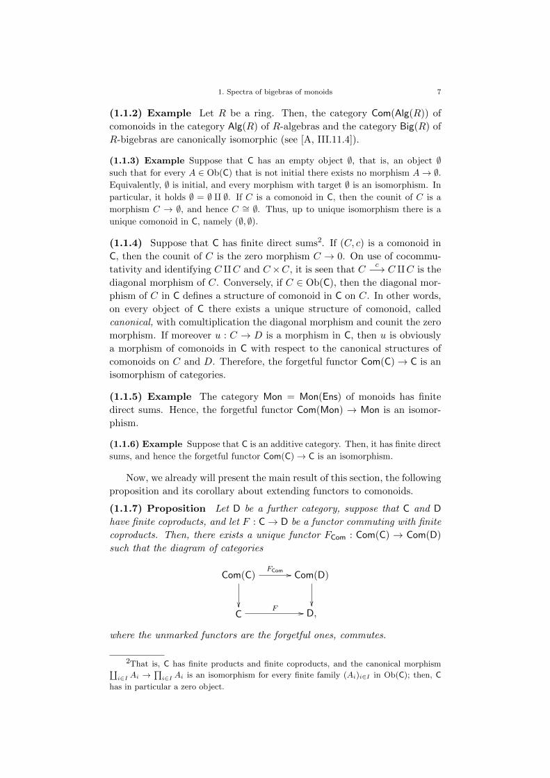
(1.1.7) Proposition Let D be a further category, suppose that C and D
have finite coproducts, and let F : C→ D be a functor commuting with finite
coproducts. Then, there exists a unique functor FCom : Com(C) → Com(D)
such that the diagram of categories
Com(C)
FCom // Com(D)
C
F // D,
where the unmarked functors are the forgetful ones, commutes.
2That is, C has finite products and finite coproducts, and the canonical morphism∐i∈I Ai →
∏i∈I Ai is an isomorphism for every finite family (Ai)i∈I in Ob(C); then, C
has in particular a zero object.
8 I. Algebras of monoids
Proof. For every comonoid A in C, the comultiplication A → A q Ainduces a morphism F (A)→ F (A) q F (A) in D that defines a structure of
comonoid in D on F (A). Moreover, if u : A→ B is a morphism in Com(C),
then F (u) : F (A)→ F (B) is obviously a morphism in Com(D) with respect
to the structure of comonoid in D on F (A) and F (B) defined as above.
(1.1.8) If, in the notation of 1.1.7, no confusion can arise, then we denote
the functor FCom by abuse of language again by F .
(1.1.9) Corollary Suppose that C has finite direct sums, let D be a cate-
gory with finite coproducts, and let F : C→ D be a functor commuting with
finite coproducts. Then, there is a unique functor FCom : C→ Com(D) such
that the diagram of categories
Com(D)
C
FCom
99ttttttttttt
F// D,
where the unmarked functor is the forgetful one, commutes.
Proof. Clear from 1.1.4 and 1.1.7.
(1.1.10) If, in the notation of 1.1.7 and 1.1.9, the functor F is contravari-
ant, we can apply the above to D to lift F uniquely to a contravariant
functor FCom : Com(C)→ Mon(D) or FCom : C→ Mon(D), respectively.
We end this section with some remarks on monomodules in arbitrary
categories. Keep in mind that by an M -monomodule we mean a structure
of M -action, where M is a monoid.
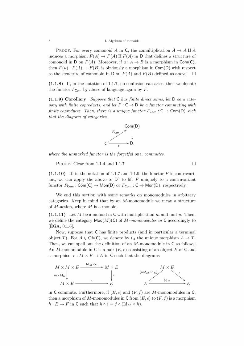
(1.1.11) Let M be a monoid in C with multiplication m and unit u. Then,
we define the category Mod(M)(C) of M -monomodules in C accordingly to
[EGA, 0.1.6].
Now, suppose that C has finite products (and in particular a terminal
object T ). For A ∈ Ob(C), we denote by tA the unique morphism A → T .
Then, we can spell out the definition of an M -monomodule in C as follows:
An M -monomodule in C is a pair (E, e) consisting of an object E of C and
a morphism e : M × E → E in C such that the diagrams
M ×M × EIdM×e //
m×IdE
M × Ee
M × Ee
##GGGGGGGGG
M × E e // E E
(utM ,IdE);;wwwwwwwww IdE // E
in C commute. Furthermore, if (E, e) and (F, f) are M -monomodules in C,
then a morphism ofM -monomodules in C from (E, e) to (F, f) is a morphism
h : E → F in C such that h e = f (IdM × h).
1. Spectra of bigebras of monoids 9
(1.1.12) Let f : M → N be a morphism in Mon(C). If E is an N -
monomodule in C, then we can consider E by means of f as an M -mo-
nomodule in C. This gives rise to a faithful functor
Mod(N)(C)→ Mod(M)(C),
called the scalar restriction functor by means of f . In particular, as every
monoid in C is a monomodule in C over itself, we can consider every monoid
in C under M as an M -monomodule in C, and this gives rise to a faithful
functor
Mon(C)/M → Mod(M)(C),
by abuse of language called the forgetful functor.
Now, suppose that C has finite products. If we denote the multiplication
of N by n, then the operation of the structure of M -monomodule underlying
N is given by n (f × IdN ) : M ×N → N .
(1.1.13) Concerning set theory, we have to consider 1.1.1. If C is a U-category,
then Mon(C) and Mod(M)(C) for a monoid M in C enjoy the same property as the
forgetful functors Mon(C)→ C and Mod(M)(C)→ C are faithful.
Moreover, if C is U-small, then so are Mon(C) and Mod(M)(C) for a monoid
M in C. Indeed, by the above we need only show that both these categories have
U-small sets of objects. In order to achieve this it suffices to show that the set of
monoids in C or M -monomodules in C, respectively, with underlying object in C a
given A ∈ Ob(C) is U-small. So, let A ∈ Ob(C). The set of structures of monoid or
in C, or M -monomodule in C, respectively, on A is a subset of HomC∧U
(hA×hA, hA),
or of HomC∧U
(hM × hA, hA), respectively, where C∧U denotes the category of U-
presheaves on C and hA and hM denote the images of A and M under the Yoneda
embedding C→ C∧U . Since C is U-small we know that C∧U is a U-category, and hence
HomC∧U
(hA× hA, hA), or HomC∧U
(hM × hA, hA), respectively, is U-small. The claim
follows from this.
Finally, if C ∈ U , then in holds Mon(C) ∈ U and Mod(M)(C) ∈ U for a monoid
M in C. Indeed, keeping the above notations it suffices to show that for every
monoid in C, or every M -monomodule in C, respectively, with underlying object
A ∈ Ob(C) the corresponding morphism hA × hA → hA, or hM × hA → hA,
respectively, in C∧U is an element of U . But as
HomC∧U
(hA × hA, hA) ⊆∏B∈Ob(C) HomEns((hA × hA)(B), hA(B)) ∈ U
by [1, I.11.1 Proposition 6, Corollaire], and similarly in the case of an M -monomo-
dule, this is clear.
Since analogous statements for C apply, we get immediately analogous state-
ments for Com(C).
1.2. Generalities on monoids
We collect here some elementary definitions and results about monoids,
used throughout the rest of the thesis.
(1.2.1) A monoid M is called cancellable if every element of M is can-
cellable, that is, if m+ k = m+ l implies k = l for all m, k, l ∈M .
10 I. Algebras of monoids
Cancellability of monoids may be characterised by monoids of differ-
ences. As these will moreover play a fundamental role in Chapter IV, we
give a short reminder.
(1.2.2) Let M be a monoid, and let T ⊆ M be a subset. We denote by
M − T the monoid of differences of M with negatives in T and by εT (M)
or, if no confusion can arise, by εT the canonical morphism M →M − T in
Mon. If N is a monoid, then the morphisms M → N in Mon that map T
into the set of invertible elements of N are precisely the morphisms M → N
in Mon that factor over εT . If T ′ is the submonoid of M generated by T ,
then it holds M − T = M − T ′. If T = t, then by abuse of language we
write M − t and εt instead of M −T and εT , respectively, and then we have
M − t = M − N0t. The above shows that εT is an epimorphism. It is a
monomorphism if and only if every element in T is cancellable.
In case T = M the above yields a left adjoint Diff : Mon → Ab of the
canonical injection Ab → Mon. The group Diff(M) is called the group of
differences of M . The monoid M is cancellable if and only if the canonical
morphism εM : M → Diff(M) is a monomorphism ([A, I.2.4]).
(1.2.3) A monoid M is called torsionfree if rm = rn implies m = n for
all m,n ∈ M and all r ∈ N. Obviously, if M is cancellable, then it is
torsionfree if and only if the group Diff(M) is torsionfree. A monoid M is
called aperiodic if the submonoid of M generated by m is infinite for every
m ∈ M \ 0, and it is called integrally closed if it is cancellable and for
every g ∈ Diff(M) such that there is an n ∈ N with ng ∈M it holds g ∈M .
The properties of being aperiodic or integrally closed will not be used
often in what follows, but we show that they are shared by those monoids
that will occur often.
(1.2.4) Proposition Let M be a monoid.
a) If M is torsionfree and cancellable, then M is aperiodic.
b) If M is torsionsfree, cancellable and finitely generated, then M is
integrally closed.
Proof. a) Let m ∈M be such that the submonoid of M generated by
m is finite. Then, there are r ∈ N0 and s ∈ N such that rm = (r + s)m.
Hence, as M is cancellable we get sm = 0, and as M is torsionfree it follows
m = 0. Therefore M is aperiodic.
b) As M is torsionfree and finitely generated, Diff(M) is a free group
with a finite basis E ⊆ M . Let g ∈ Diff(M) and n ∈ N be such that
ng ∈ M . Then, there are families (ae)e∈E , (be)e∈E and (ce)e∈E in N0 with
g =∑
e∈E(ae − be)e and ng =∑
e∈E cee. Hence, we have∑e∈E n(ae − be)e =
∑e∈E cee.
As E is a basis of Diff(G), we get n(ae − be) = ce and thus ae − be ∈ N0 for
every e ∈ E. This implies g ∈M , and therefore M is integrally closed.
1. Spectra of bigebras of monoids 11
As with rings, there are notions of ideals and prime ideals of monoids.
These may help to exhibit a strong analogy between rings and monoids,
only part of which will surface here. We will use the notion of prime ideal
of monoids merely as a technical tool in 1.3.16.
(1.2.5) Let M be a monoid. A monoideal of M is a sub-M -monomodule
of the M -monomodule underlying M , that is, a subset A ⊆ M such that
M + A ⊆ A. We denote by IM the set of monoideals of M , furnished with
the ordering induced by ⊆.
A monoideal A ⊆ M is called prime if M \ A is a submonoid of M . If
A ⊆M is a prime monoideal and N ⊆M is a submonoid with A ⊆ N , then
A is a prime monoideal of N .
(1.2.6) Example Let E be a set. We furnish the free monoid N⊕E0 over
E with the ordering induced by the product ordering on NE0 . Then, it is
clear that a subset A ⊆ N⊕E0 is a monoideal of N⊕E0 if and only if for every
x ∈ A and every y ∈ N⊕E0 with x ≤ y it holds y ∈ A. In particular, every
monoideal of N⊕E0 is generated by the set of its minimal elements.
Carrying further the analogy between rings and monoids mentioned
above we show next that this fits with the notion of Noetherianity.
(1.2.7) A monoid M is called Noetherian if the ordered set IM of monoide-
als of M is Noetherian3. This holds if and only if every monoideal of M is
finitely generated, as is easily seen.
(1.2.8) Proposition If E is a set, then the free monoid N⊕E0 over E is
Noetherian if and only if E is finite.
Proof. If E is infinite, then the monoideal generated by E is obviously
not finitely generated and hence N⊕E0 is not Noetherian. For the converse
it suffices by 1.2.6 to show that for every n ∈ N0 every antichain4 in Nn0 ,
furnished with the product ordering, is finite. This we do by induction on
n.
For n ≤ 1 it is obvious. So, let n > 1, suppose that every antichain in
Nn−10 is finite, and assume that there is an infinite antichain A ⊆ Nn
0 . We
identify Nn0 with Nn−1
0 ⊕ N0 and denote by p and q respectively the first
and the second canonical projection, and we set B := p(A). If x, y ∈ A are
such that p(x) = p(y), then comparability of q(x) and q(y) implies x = y.
Thus, the restriction of p to A is injective, and therefore B is infinite.
Using the fact that the set of minimal elements of a nonempty subset of
Nn−10 is nonempty and finite, we can recursively define a strictly increasing
3An ordered set E is called Noetherian if every increasing sequence in E is stationary.
This is the case if and only if every nonempty subset of E has a maximal element ([E,
III.7.5 Proposition 6]).4To avoid confusion we call a subset of an ordered set E an antichain (in E) if it is
free (in the terminology of [E]), that is, if its elements are pairwise incomparable.
12 I. Algebras of monoids
sequence (bi)i∈N0 in B such that x ∈ B | bi < x is infinite for every
i ∈ N0 as follows. First, there exists a minimal element b0 of B such that
x ∈ B | b0 < x is infinite. Next, if i ∈ N0 and if bi ∈ B is such that
x ∈ B | bi < x is infinite, then there exists a minimal element bi+1 of this
set such that x ∈ B | bi+1 < x is infinite.
For every i ∈ N0 there is a unique preimage ai ∈ A of bi under p.
As A is an antichain, the elements ai and ai+1 are incomparable for every
i ∈ N0, and therefore p(ai) < p(ai+1) implies q(ai) > q(ai+1). But this
yields the contradiction that (q(ai))i∈N0 is a strictly decreasing sequence in
the well-ordered set N0, and thus the claim is proven.
A well-known defect of the category Ann of rings is, that a morphism
that is a mono- and an epimorphism is not necessarily an isomorphism.
In the category Mon of monoids the same defect occurs, and the standard
counterexample is essentially the same as in Ann.
(1.2.9) A morphism in Mon is a monomorphism if and only if its underlying
map is injective. Indeed, let f : M → N be a monomorphism in Mon and
consider the submonoid L := (x, y) ∈ M2 | f(x) = f(y) of M2. If we
denote by p1 and p2 the restrictions to L of the canonical projections of
M2, we get f p1 = f p2, and as f is a monomorphism this implies that
p1 = p2. From this it is easily seen that the map underlying f is injective.
The converse is obvious.
A morphism in Mon is an epimorphism if its underlying map is surjec-
tive, but the converse does not necessarily hold. Indeed, the first statement
is obvious. A counterexample for its converse is given by the canonical in-
jection from the additive monoid N0 into its group of differences Z which is
an epimorphism by 1.2.2 but obviously not surjective.
(1.2.10) Lemma Let M be a group, and let N,P,Q ⊆ M be submonoids
such that P ∪ (−P ) ⊆ Q. Then, it holds (N + P ) ∩Q = (N ∩Q) + P .
Proof. For x ∈ N and y ∈ P with x + y ∈ Q we have −y ∈ Q, hence
x = x + y − y ∈ Q and therefore x + y ∈ (N ∩ Q) + P . Conversely, for
x ∈ N ∩ Q and y ∈ P we have y ∈ Q, hence x + y ∈ Q and therefore
x+ y ∈ (N + P ) ∩Q.
1.3. Algebras and bigebras of monoids
For a ring R we define the functor R[•] of algebras of monoids over R as
adjoint to some forgetful functor, and then we vary R to obtain a bifunctor
[•] from Ann×Mon to Ann. By doing so we lose the structure of R-algebra
on the rings R[M ]. Keeping track of this structure amounts to consider [•]as a bifunctor over the first projection of Ann ×Mon, and this is what we
do in this and similar situations.
1. Spectra of bigebras of monoids 13
(1.3.1) Let R be a ring. The forgetful functor Alg(R) → Mon, mapping
an R-algebra onto its underlying multiplicative monoid, has a left adjoint
denoted by
R[•] : Mon→ Alg(R).
If M is a monoid, then the R-algebra R[M ] is called the algebra of M
over R and can be constructed as follows. The R-module underlying R[M ] is
the free R-module with basis the set underlying M , and hence it is furnished
with a map e : M → R[M ] that is injective if and only if R 6= 0 or M = 0.
In this case we transport the structure of monoid of M to the basis e(M)
of R[M ] and thus get a structure of R-algebra on R[M ], and otherwise we
furnish R[M ] = 0 with its unique structure of R-algebra.
In the above notations, we denote by TR,M := e(M) the canonical basis
of R[M ] and by expR,M : M → TR,M the canonical surjection. If no con-
fusion can arise, then we set em := expR,M (m) for every m ∈M and hence
write the canonical basis of R[M ] as em | m ∈ M. Then, the multipli-
cation of R[M ] is the morphism R[M ] ⊗R R[M ] → R[M ] in Mod(R) with
em ⊗ en 7→ em+n for all m,n ∈ M , and the unit of R[M ] is the morphism
R→ R[M ] in Mod(R) with 1R 7→ e0.
An element of TR,M is called a monomial in R[M ], and a product of an
element of R and a monomial in R[M ] is called a term in R[M ] ([A, III.2.6]).
(1.3.2) Let M be a monoid. If h : R→ R′ is a morphism in Ann, then we
consider R′ and R′[M ] by means of h as R-algebras, and then the canonical
morphism M → R′[M ], m 7→ em in Mon induces by 1.3.1 a morphism
h[M ] : R[M ]→ R′[M ] in Alg(R). This gives rise to a functor
•[M ] : Ann→ Ann.
Since this maps a ring R onto the R-algebra R[M ], we also get a morphism
of functors IdAnn(•) → •[M ] and thus can consider •[M ] as a functor from
Ann to Ann under IdAlg(R).
If again h : R → R′ is a morphism in Ann, then the induced morphism
h[M ] : R[M ] → R′[M ] in Ann induces by restriction and coastriction a
morphism
Th,M : TR,M → TR′,M , em 7→ em
in Mon such that Th,M expR,M = expR′,M . This is an isomorphism if and
only if R 6= 0 and R′ 6= 0, or M = 0, and in this case its inverse equals
expR,M exp−1R′,M . The above gives rise to a functor
T•,M : Ann→ Mon
under the constant functor Ann → Mon with value M , and T•,M is a sub-
functor of the composition of •[M ] with the forgetful functor Ann → Mon
mapping a ring onto its underlying multiplicative monoid.
14 I. Algebras of monoids
(1.3.3) It follows from 1.3.1 and 1.3.2 that the functors •[M ] : Ann→ Ann
under IdAnn for varying monoids M give rise to a bifunctor
•[ ] : Ann×Mon→ Ann
under the canonical projection pr1 : Ann×Mon→ Ann.
Now, we can apply the results from 1.1 in order to turn our algebras of
monoids into bigebras of monoids in a canonical way.
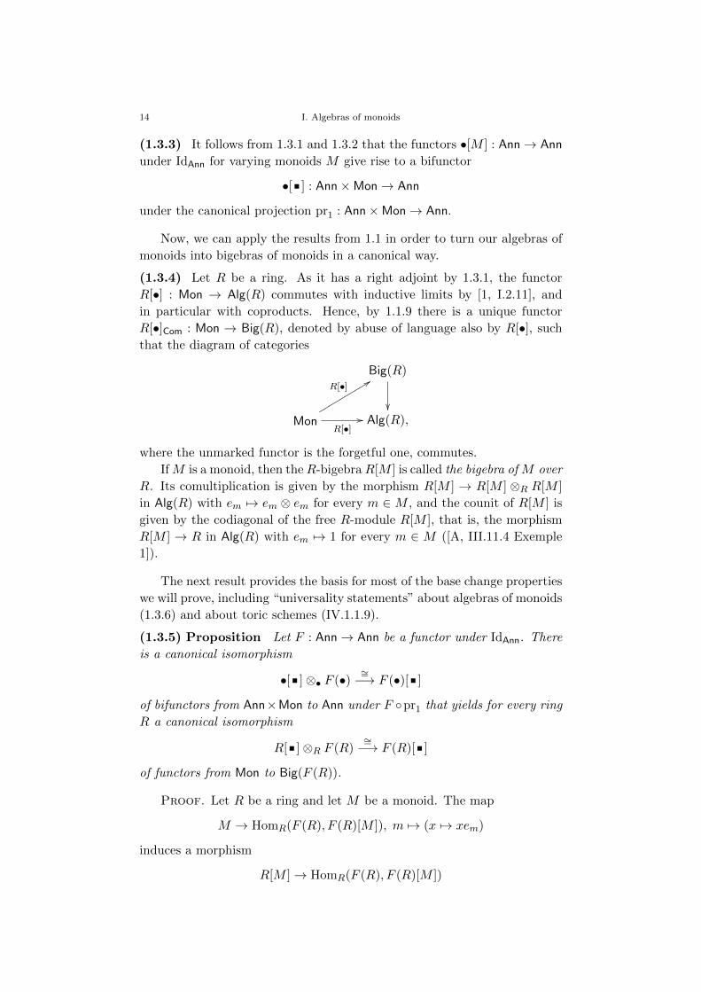
(1.3.4) Let R be a ring. As it has a right adjoint by 1.3.1, the functor
R[•] : Mon → Alg(R) commutes with inductive limits by [1, I.2.11], and
in particular with coproducts. Hence, by 1.1.9 there is a unique functor
R[•]Com : Mon → Big(R), denoted by abuse of language also by R[•], such
that the diagram of categories
Big(R)
Mon
R[•]99rrrrrrrrrr
R[•]// Alg(R),
where the unmarked functor is the forgetful one, commutes.
IfM is a monoid, then theR-bigebraR[M ] is called the bigebra of M over
R. Its comultiplication is given by the morphism R[M ] → R[M ] ⊗R R[M ]
in Alg(R) with em 7→ em ⊗ em for every m ∈ M , and the counit of R[M ] is
given by the codiagonal of the free R-module R[M ], that is, the morphism
R[M ] → R in Alg(R) with em 7→ 1 for every m ∈ M ([A, III.11.4 Exemple
1]).
The next result provides the basis for most of the base change properties
we will prove, including “universality statements” about algebras of monoids
(1.3.6) and about toric schemes (IV.1.1.9).
(1.3.5) Proposition Let F : Ann→ Ann be a functor under IdAnn. There
is a canonical isomorphism
•[ ]⊗• F (•)∼=−→ F (•)[ ]
of bifunctors from Ann×Mon to Ann under F pr1 that yields for every ring
R a canonical isomorphism
R[ ]⊗R F (R)∼=−→ F (R)[ ]
of functors from Mon to Big(F (R)).
Proof. Let R be a ring and let M be a monoid. The map
M → HomR(F (R), F (R)[M ]), m 7→ (x 7→ xem)
induces a morphism
R[M ]→ HomR(F (R), F (R)[M ])
1. Spectra of bigebras of monoids 15
in Mod(R) with em 7→ (x 7→ xem) for every m ∈ M and hence a morphism
α(R,M) : R[M ]⊗R F (R)→ F (R)[M ] in Mod(R) with α(R,M)(em ⊗ x) =
xem for every m ∈M and every x ∈ F (R). This is a morphism in Big(F (R)),
as is readily checked. On the other hand, the map
M → R[M ]⊗R F (R), m 7→ em ⊗ 1
is a morphism in Mon with target the multiplicative monoid underlying
R[M ]⊗RF (R), and hence it induces a morphism F (R)[M ]→ R[M ]⊗RF (R)
in Alg(R) with em 7→ em ⊗ 1 for every m ∈ M . Clearly, this is inverse to
the map underlying α(R,M), and since bijective morphisms in Big(F (R))
are isomorphisms it follows that α(R,M) is an isomorphism in Big(F (R)).
Finally, it is easily seen that α(R,M) is natural in R and M , and this
yields the claim.
(1.3.6) Corollary Let R be a ring, and let R′ be an R-algebra. Then,
there is a canonical isomorphism
R[•]⊗R R′∼=−→ R′[•]
of functors from Mon to Big(R′).
Proof. Clear from 1.3.5 with F (R) = R′.
(1.3.7) Corollary Let R be a ring.
a) If a ⊆ R is an ideal, then there is a canonical isomorphism
R[•]/(aR[•])∼=−→ (R/a)[•]
of functors from Mon to Big(R/a).
b) If S ⊆ R is a subset, then there is a canonical isomorphism
S−1(R[•])∼=−→ (S−1R)[•]
of functors from Mon to Big(S−1R).
Proof. Apply 1.3.6 with R′ = R/a and R′ = S−1R respectively.
(1.3.8) Corollary For every k ∈ N0 there is an isomorphism
•[k⊕i=1
i]∼=−→ •[ 1] · · · [ k]
of (k+ 1)-functors from Ann×Monk to Ann under pr1 that yields for every
ring R a canonical isomorphism
R[
k⊕i=1
i]∼=−→ R[ 1] · · · [ k]
of k-functors from Monk to Big(R).
16 I. Algebras of monoids
Proof. Let M be a monoid. Keeping in mind that •[ ] commutes
with coproducts in the second argument by 1.3.1 and applying 1.3.5 with
F ( ) = [M ], we get isomorphisms
•[ ⊕M ] ∼= •[ ]⊗• •[M ] ∼= •[M ][ ].
As these are clearly natural in M , the claim follows by induction on k.
(1.3.9) Let (I,≤) be a preordered set, and let M = ((Mi)i∈I , (pij)i≤j) be
a projective system in Mon over I. For a ring R, we can compose M with
R[•] : Mon→ Big(R) to obtain a projective system
R[M] = ((R[Mi])i∈I , (R[pij ])i≤j)
in Big(R) over I, and analogously for R[•] : Mon → Alg(R). For an R-
algebra R′, it follows from 1.3.6 that there is a canonical isomorphism
R[M]⊗R R′ ∼= R′[M]
of projective systems in Big(R′) (or in Alg(R′)).
Furthermore, the bifunctor •[ ] : Ann × Mon → Ann under pr1 corre-
sponds to a functor from Mon to Hom(Ann,Ann)/IdAnn . Composing this with
M we get a projective system
•[M] =((•[Mi])i∈I , (•[pij ])i≤j
)of functors from Ann to Ann under IdAnn over I.
The following notion of restricted Noetherianity unifies the notions of
monomial ideal and graded ideal (see III.3.3.1).
(1.3.10) Let R be a ring, let E be an R-module, and let L ⊆ E be a
subset. A sub-R-module F ⊆ E is called L-generated if it has a generating
set contained in L, and finitely L-generated if it has a finite generating
set contained in L. The sum of a (finite) family of (finitely) L-generated
sub-R-modules of E is (finitely) L-generated again.
Moreover, E is called L-Noetherian if the set of all L-generated sub-
R-modules of E, ordered by inclusion, is Noetherian. Clearly, E is L-
Noetherian if and only if every L-generated sub-R-module of E is finitely
L-generated. If E is L-Noetherian, then every sub-R-module of E that
contains L is L-Noetherian, too. If L ⊆ R, then the ring R is called L-
Noetherian if it is L-Noetherian considered as an R-module.
(1.3.11) Let M be a monoid, and let R be a ring. We denote by IR,M the
set of TR,M -generated ideals of R[M ], furnished with the ordering induced
by ⊆. The morphism expR,M in Mon induces a morphism
ExpR,M : IM → IR,M , A 7→ 〈expR,M (A)〉R[M ]
in Ord that is an isomorphism if and only if R 6= 0 and R′ 6= 0, or M = 0,
and then its inverse is given by a 7→ exp−1R,M (a ∩TR,M ).
1. Spectra of bigebras of monoids 17
Now, let h : R → R′ be a morphism in Ann. Then, mapping a TR,M -
generated ideal a ⊆ R[M ] onto the image of the canonical morphism
a⊗R[M ] R′[M ]→ R′[M ]
in Mod(R′[M ]) defines a morphism Ih,M : IR,M → IR′,M in Ord with
Ih,M ExpR,M = ExpR′,M .
In particular, Ih,M is an isomorphism if and only if R 6= 0 and R′ 6= 0, or
M = 0. The above gives rise to a functor I•,M : Ann → Ord under the
constant functor Ann→ Ord with value IM .
Finally, let A ⊆ M be a monoideal, and let h : R → R′ be a morphism
in Ann. Then, h[M ] : R[M ]→ R′[M ] induces by restriction and coastriction
a morphism ExpR,M (A) → ExpR′,M (A) in Mod(R). This gives rise to a
functor Exp•,M (A) : Ann → Ab that is a subfunctor of the composition
of •[M ] with the forgetful functor Ann → Ab which maps a ring onto its
underlying additive group.
(1.3.12) Example Let E be a set, let M = N⊕E0 be the free monoid with
basis E, and let R be a ring. Then, the R-algebra R[M ] is the polynomial
algebra in Card(E) indeterminates over R. If no confusion can arise we
write TR,E := TR,N⊕E0for the monoid of monomials in R[M ]. If h : R→ R′
is a morphism in Ann and A ⊆ M is a monoideal, then 1.3.11 allows us to
identify the R′[M ]-module ExpR,M (A)⊗R[M ]R′[M ] with its canonical image
in R′[M ] and in particular consider it as an ideal of R′[M ], and then it holds
ExpR,M (A)⊗R[M ] R′[M ] = ExpR′,M (A).
(1.3.13) Proposition Let R be a ring, and let u : M → N be a mor-
phism in Mon. If R 6= 0, then u is an epimorphism or a monomorphism,
respectively, if and only if R[u] is so.
Proof. As R[•] has a right adjoint by 1.3.1 it preserves epimorphisms.
Conversely, suppose that R[u] is an epimorphism, and let v, w : N → P be
morphisms in Mon with v u = w u. It follows R[v] R[u] = R[w] R[u],
and in particular these two morphisms coincide on em for every m ∈ M .
Hence, since R 6= 0 we get v = w, and thus u is an epimorphism.
Next, we suppose that u is a monomorphism and show that Ker(R[u]) =
0. Let (rm)m∈M be a family of finite support in R with R[u](∑
m∈M rmem) =
0 and hence∑
m∈M rmeu(m) = 0. As u is injective by 1.2.9, the family
(eu(m))m∈M in R[N ] is free. Therefore, it holds rm = 0 for every m ∈M , and
from this we see that Ker(R[u]) = 0. Conversely, if R[u] is a monomorphism,
then its restriction to the set em | m ∈ M is injective, and hence u is a
monomorphism, for R 6= 0.
Next, we consider rings of fractions of algebras of monoids. There is an
obvious distinction whether the set of denominators consists only of mono-
mials (1.3.14) or not (1.3.15).
18 I. Algebras of monoids
(1.3.14) Let M be a monoid, and let T ⊆ M be a subset. Then, we have
morphisms
•[εT ] : •[M ]→ •[M − T ]
and
ηexp•,M (T ) : •[M ]→ exp•,M (T )−1(•[M ])
of functors from Ann to Ann under IdAnn.
If R is a ring, then R[εT ] maps expR,M (T ) into the set of invertible
elements of R[M − T ], and hence corresponds to a morphism
u : expR,M (T )−1(R[M ])→ R[M − T ]
in Alg(R[M ]) that is readily seen to be natural in R. On the other hand,
the morphism from M to the multiplicative monoid underlying the ring
expR,M (T )−1(R[M ]) that maps an element m onto the canonical image of
em in expR,M (T )−1(R[M ]) maps T into the set of invertible elements of
expR,M (T )−1(R[M ]). Therefore, it factors over εT and thus induces a mor-
phism R[M −T ]→ expR,M (T )−1(R[M ]) in Alg(R[M ]) that is easily seen to
be inverse to u. Thus, the functors •[M − T ] and exp•,M (T )−1(•[M ]) from
Ann to Ann under •[M ] are canonically isomorphic.
(1.3.15) Let R be a ring, let M be a monoid, and let S ⊆ R[M ] be a subset.
We set T := S ∩R, denote by ηS : R[M ]→ S−1(R[M ]) and ηT : R→ T−1R
the canonical morphisms in Ann, and set U := ηT [M ](S) ⊆ (T−1R)[M ].
Moreover, we denote by i : R → R[M ], j : T−1R → (T−1R)[M ], and
ηU : (T−1R)[M ]→ U−1((T−1R)[M ]) the canonical morphisms in Ann.
Then, there are morphisms f, g, h in Ann such that the diagrams
RηT //
i
T−1Rj //
f
(T−1R)[M ]
ηU
R[M ]ηS // S−1(R[M ]) U−1((T−1R)[M ])
goo
and
Ri //
ηT
R[M ]ηS //
ηT [M ]
S−1(R[M ])
h
T−1Rj // (T−1R)[M ]
ηU // U−1((T−1R)[M ])
in Ann commute. It is readily checked that g and h are mutually inverse,
and hence the R[M ]-algebras
R[M ]ηS−→ S−1(R[M ])
and
R[M ]ηUηT [M ]−−−−−−→ U−1((T−1R)[M ])
are isomorphic.
We end this section with a construction used in IV.1.3.2 for the investi-
gation of properness of toric schemes.
1. Spectra of bigebras of monoids 19
(1.3.16) Let M be a monoid, let P ⊆M be a prime monoideal, and let R
be a ring. We define a map
M → R[M \ P ], x 7→
ex, if x ∈M \ P ;
0, if x ∈ P.
Since P is prime it is easy to see that this is a morphism in Mon from M
to the multiplicative monoid underlying R[N ] and hence corresponds to a
morphism
ϑM,P (R) : R[M ]→ R[M \ P ], ex 7→
ex, if x /∈ P ;
0, if x ∈ P
in Alg(R). Obviously, ϑM,P (R) is surjective. Moreover, it is clearly natural
in R and hence gives rise to a morphism ϑM,P : •[M ]→ •[M \P ] of functors
from Ann to Ann under IdAnn.
Now, let L be a submonoid of M with P ⊆ L. Then, P is a prime
monoideal of L, and hence L \ P is a submonoid of M \ P . Moreover, the
diagram
•[M ]ϑM,P // •[M \ P ]
•[L]ϑL,P //
OO
OO
•[L \ P ],
OO
OO
of functors from Ann to Ann under IdAnn, where the unmarked morphisms
are induced by the canonical injections of L and L \ P into M and M \ P ,
commutes.
1.4. Spectra of algebras and bigebras of monoids
In this section we translate the above into geometry by taking spectra.
In this way, bigebra structures turn into monoid schemes and monomodule
schemes.
(1.4.1) Let R be a ring. The contravariant functor Spec from Alg(R)
to Sch/R commutes with coproducts. Hence, by 1.1.10 there is a unique
contravariant functor SpecCom : Big(R)→ Mon(Sch/R), by abuse of language
also denoted by Spec, such that the diagram of categories
Big(R)Spec //
Mon(Sch/R)
Alg(R)
Spec // Sch/R,
where the unmarked functors are the forgetful ones, commutes.
If A is an R-bigebra with comultiplication c : A → A ⊗R A and counit
e : A→ R, then the multiplication and the unit of the structure of monoid
20 I. Algebras of monoids
R-scheme on Spec(A) are given by the morphisms of R-schemes
Spec(c) : Spec(A)×R Spec(A)→ Spec(A)
and
Spec(e) : Spec(R)→ Spec(A),
respectively.
(1.4.2) LetR be a ring, and let A be anR-bigebra. Then, the contravariant
functor
Spec : Big(R)→ Mon(Sch/R)
from 1.4.1 induces a contravariant functor
Spec : Big(R)/A → Mon(Sch/R)/ Spec(A).
Its composition with the forgetful functor
Mon(Sch/R)/ Spec(A) → Mod(Spec(A))(Sch/R)
(see 1.1.12) yields a contravariant functor
Big(R)/A → Mod(Spec(A))(Sch/R).
If h : B → A is an R-bigebra over A with comultiplication d, then it
is seen from 1.1.11 that the Spec(A)-action of the structure of Spec(A)-
monomodule R-scheme on Spec(B) is given by
Spec((h⊗ IdB) d)) : Spec(A)×R Spec(B)→ Spec(B).
(1.4.3) If R is a ring, then composition of R[•] : Mon → Alg(R) with
Spec : Alg(R)→ Sch/R yields a contravariant functor
Spec(R[•]) : Mon→ Sch/R.
Moreover, if M is a monoid, then composition of •[M ] : Ann → Ann
under IdAnn with Spec : Ann→ Sch yields a contravariant functor
Spec(•[M ]) : Ann→ Sch
over Spec.
Finally, composition of the bifunctor •[ ] : Ann×Mon→ Ann under the
canonical projection pr1 : Ann ×Mon → Ann with Spec : Ann → Sch yields
a contravariant bifunctor
Spec(•[ ]) : Ann×Mon→ Sch
over Spec pr1.
(1.4.4) Let R be a ring. Then, composition of R[•] : Mon → Big(R) with
Spec : Big(R)→ Mon(Sch/R) yields a contravariant functor
Spec(R[•]) : Mon→ Mon(Sch/R).
1. Spectra of bigebras of monoids 21
If u : N → M is a morphism in Mon, then this contravariant functor
maps u onto the morphism
Spec(R[u]) : Spec(R[M ])→ Spec(R[N ])
in Mon(Sch/R) and hence by 1.4.2 defines on Spec(R[N ]) a structure of
Spec(R[M ])-monomodule R-scheme. Thus, for a monoid M the above de-
fines a contravariant functor
Spec(R[•]) : Mon/M → Mod(Spec(R[M ]))(Sch/R).
(1.4.5) Proposition Let F : Ann → Ann be a functor over IdAnn. Then,
there is a canonical isomorphism
Spec(•[ ])×Spec(•) Spec(F (•))∼=−→ Spec(F (•)[ ])
of contravariant bifunctors from Ann×Mon to Sch under Spec F pr1 that
yields for every ring R a canonical isomorphism
Spec(R[ ])×R F (R)∼=−→ Spec(F (R)[ ])
of contravariant functors from Mon to Mon(Sch/R).
Proof. This follows immediately from 1.3.5 and 1.4.4.
(1.4.6) Corollary Let R be a ring, and let R′ be an R-algebra. Then,
there is a canonical isomorphism
Spec(R[•])×R R′∼=−→ Spec(R′[•])
of contravariant functors from Mon to Mon(Sch/R′).
Proof. Clear from 1.4.5 (or from 1.3.6 and 1.4.4).
(1.4.7) Let I be a preordered set, and let M = ((Mi)i∈I , (pij)i≤j) be a
projective system in Mon over I. For i ∈ I we set
XM,i := Spec(•[Mi]) : Ann→ Sch
and denote by tM,i : XM,i(•) → Spec(•) the canonical morphism, and for
i, j ∈ I with i ≤ j we set
ιM,i,j(•) := Spec(•[pij ]) : XM,i(•)→ XM,j(•).
If R is a ring, then composing the projective system R[M] in Big(R) over
I with Spec : Big(R)→ Mon(Sch/R) yields an inductive system
Spec(R[M]) =((XM,i(R))i∈I , (ιM,i,j(R))i≤j
)in Mon(Sch/R) over I, and analogously for Spec : Alg(R) → Sch/R. For an
R-algebra R′, it follows from 1.3.9 that there is a canonical isomorphism
Spec(R[M])×R R′ ∼= Spec(R′[M])
of inductive systems in Mon(Sch/R′) (or in Sch/R′).
22 I. Algebras of monoids
Furthermore, composing the projective system •[M] of functors from
Ann to Ann under IdAnn over I with Spec : Ann → Sch we get an inductive
system
Spec(•[M]) =((XM,i(•))i∈I , (ιM,i,j(•))i≤j
)of contravariant functors from Ann to Sch over Spec over I.
As was said above, our aim is to somehow glue the schemes defined by
a projective system M of monoids. The next task is to make sense of this
aim.
(1.4.8) Let R be a ring, let I be a preordered set, and letM be a projective
system in Mon over I. We say that M is openly immersive for R if ιM,i,j(R)
is an open immersion for all i, j ∈ I with i ≤ j. If R′ is an R-algebra
and M is openly immersive for R, then 1.4.7 implies that it is also openly
immersive for R′, since open immersions are stable under base change by
[EGA, I.4.3.6]. We say that M is openly immersive if it is openly immersive
for Z, or – equivalently – if ιM,i,j is an open immersion for all i, j ∈ I with
i ≤ j.
(1.4.9) Let X be a set, and let (Xi)i∈I be a covering of X. On use of the
canonical isomorphism between the category of lower semilattices and mor-
phisms of lower semilattices5 and the category of idempotent, commutative,
associative magmas (see [A, I.1 Exercise 15]) it is easily seen that if (Xi)i∈Iis injective, then there exists at most one structure of a lower semilattice on
I such that for all i, j ∈ I it holds Xi ∩Xj = Xinf(i,j). If (Xi)i∈I is injective
and there exists such a structure, then (Xi)i∈I is said to have the intersec-
tion property, and then we consider I as a lower semilattice, furnished with
the uniquely determined structure described above. Now, suppose we are
given a structure of lower semilattice on I such that Xi ∩Xj = Xinf(i,j) for
all i, j ∈ I. If no confusion can arise, then by abuse of language (Xi)i∈I is
also said to have the intersection property, even if it is not injective.
If C is category and G is a functor or a contravariant functor from C
to Sch/S , then by abuse of language an open covering (ui : Fi → G)i∈Iof G is said to have the intersection property if (ui(C)(Fi(C)))i∈I has the
intersection property for every C ∈ Ob(C).
(1.4.10) Let R be a ring, let I be a lower semilattice, and let M be a
projective system in Mon over I that is openly immersive for R. Moreover,
let R′ be an R-algebra. Then, it follows from 1.4.8 and [EGA, I.2.4.1;
0.4.1.7] that the family (XM,i(R′))i∈I of R′-schemes can be glued along
(XM,inf(i,j)(R′))(i,j)∈I2 to obtain an R′-scheme
tM(R′) : XM(R′)→ Spec(R′)
5An ordered set E is called a lower semilattice if inf(x, y) exists for all x, y ∈ E. If
E and F are lower semilattices, then a morphism of lower semilattices from E to F is a
morphism f : E → F in Ord such that f(inf(x, y)) = inf(f(x), f(y)) for all x, y ∈ E.
1. Spectra of bigebras of monoids 23
together with open immersions ιM,i(R′) : XM,i(R
′) XM(R′) in Sch/R′ for
all i ∈ I such that, identifying XM,i(R′) with its image under ιM,i(R
′) for
every i ∈ I, the family (XM,i(R′))i∈I is an affine open covering of XM(R′)
that has the intersection property.
The above gives rise to a contravariant functor
XM : Alg(R)→ Sch/R
over Spec together with open immersions ιM,i : XM,i → XM of such con-
travariant functors. If R′ is an R-algebra, then it follows from 1.4.7 that the
diagram of categories
Alg(R′)XM // Sch/R′
Alg(R)XM //
•⊗RR′OO
Sch/R
•×RR′OO
commutes up to canonical isomorphism.
(1.4.11) Example Let R be a ring, let I be a lower semilattice, and let
M be a projective system in Mon over I that is openly immersive. Then, it
holds XM(R) = ∅ if and only if I = ∅ or R = 0. Indeed, if XM(R) = ∅ and
I 6= ∅, then there is an i ∈ I with R[Mi] = 0, hence R = 0, or Mi = 0 and
therefore R = R[Mi] = 0. The converse holds obviously.
Besides the underlying schemes we would also like to glue the algebraic
structures on the affine pieces of the schemes defined by a projective system
M of monoids. This does not lead to any problems and will be done next.
(1.4.12) Let R be a ring, let Y be a monoid R-scheme, let X be an R-
scheme, and let (Xi)i∈I be an open covering of X. Moreover, suppose for
every i ∈ I that Xi is furnished with a structure of Y -monomodule R-scheme
that induces for every j ∈ I a structure of sub-Y -monomodule R-scheme on
Xi∩Xj , and that for i, j ∈ I the structures on Xi∩Xj induces by Xi and Xj
coincide. Then, there is unique structure of Y -monomodule R-scheme on X
that induces for every i ∈ I on Xi the given structure of Y -monomodule R-
scheme. Indeed, for every i ∈ I the Y -action on Xi induces by composition
a morphism Y ×Xi → X in Sch/R, and since (Y ×Xi)i∈I is an open covering
of Y ×X these morphisms define a unique morphism Y ×X → X with the
desired properties.
(1.4.13) Let R be a ring, let I be a lower semilattice with a smallest
element ω, and let M be a projective system in Mon over I that is openly
immersive for R. Moreover, let R′ be an R-algebra. Then, Spec(R′[M]) is
an inductive system in Mon(Sch/R′)/XM,ω(R)over I, and hence composition
with the forgetful functor
Mon(Sch/R′)/XM,ω(R′) → Mod(XM(R′))(Sch/R′)
24 I. Algebras of monoids
(1.4.2) yields an inductive system in Mod(XM(R′))(Sch/R′) over I. Hence,
keeping in mind 1.4.10 we can apply 1.4.12 to obtain a structure ofXM,ω(R′)-
monomodule R′-scheme on XM(R′) that induces for every i ∈ I the structure
of XM,ω(R′)-monomodule R′-scheme on XM,i(R′) obtained by applying the
forgetful functor to its structure of monoid R′-scheme under XM,ω(R′).
If R′′ is an R′-algebra, then we can identify the monoid R′′-schemes
XM,ω(R′)×R′ R′′ and XM,ω(R′′) by 1.4.6, and doing this it is easily seen by
1.4.10 that there is a canonical isomorphism
XM(R′)×R′ R′′ ∼= XM(R′′)
of XM,ω(R′′)-monomodule R′′-schemes.
In order to illustrate the above we describe a certain type of openly
immersive projective system of monoids. Below, instances of this type will
give rise to toric schemes.
(1.4.14) Proposition Let M be a monoid, and let t ∈M . Then,
Spec(•[εt]) : Spec(•[M − t])→ Spec(•[M ])
is an open immersion of contravariant functors from Ann to Sch.
Proof. Let R be a ring. The R[M ]-algebras R[εt] : R[M ]→ R[M − t]and ηet : R[M ]→ R[N ]et are canonically isomorphic by 1.3.14, and thus the
claim follows from [EGA, I.1.6.6].
(1.4.15) Example Let I be a lower semilattice with a smallest element ω,
and let M = ((Mi)i∈I , (pij)i≤j) be a projective system in Mon over I such
that for all i, j ∈ I with i ≤ j there is a tij ∈ Mj such that Mi = Mj − tijand pij = εtij . Then, by 1.4.14 it is seen that M is openly immersive and
hence gives rise to a functor XM : Ann→ Sch over Spec that maps a ring R
onto the XM,ω(R)-monomodule R-scheme XM,ω(R).
(1.4.16) Concerning set theory, we have to consider 1.4.10. So, suppose that I is
U-small, that M = (Mi)i∈I takes values in the category Mon of monoids that are
elements of U (or only that the values of M are monoids with a U-small underlying
set), and that R′ ∈ U (or only that the underlying set of R′ is U-small). Then, it
holds XM(R′) ∈ U . Indeed, we have to show that the underlying set of XM(R′) and
the sets underlying the values of the structure sheaf of XM(R′) are elements of U .
The second claim follows immediately from [1, I.11.2] and [EGA, 0.3.3.1; 0.3.2.1],
and since our hypotheses imply R′[Mi] ∈ U and hence XM,i(R′) ∈ U for every
i ∈ I, the first claim follows from [1, I.11.1 Proposition 1, Corollaire; Proposition
4, Corollaire 2].
2. Geometric properties of algebras of monoids 25
2. Geometric properties of algebras of monoids
Let R be a ring.
2.1. Separatedness and finiteness conditions
We start describing the geometry of spectra of algebras of monoids,
or more generally of schemes of the form XM(R), by looking at the basic
properties of quasiseparatedness, separatedness, and quasicompactness. The
schemes XM(R) are always quasiseparated, but not necessarily separated.
We characterise separatedness independently of R and only in terms of the
projective system of monoids M.
(2.1.1) Lemma Let X be a scheme, and let (Xi)i∈I be an affine open
covering of X. Then, it holds:
a) If (Xi)i∈I has the intersection property, then X is quasiseparated.
b) If (Xi)i∈I has the intersection property, then X is separated if and
only if for all i, j ∈ I the ring OX(Xinf(i,j)) is generated by the union of the
canonical images of OX(Xi) and OX(Xj).
c) If I is finite, then X is quasicompact.
Proof. a) holds by [EGA, I.6.1.2], b) follows from [EGA, I.5.3.6], and
c) is obvious.
(2.1.2) Proposition Let M = ((Mi)i∈I , (pij)i≤j) be a projective system
in Mon over a lower semilattice I, and suppose that M is openly immersive
for R.
a) XM(R) is quasiseparated.
b) If R 6= 0, then XM(R) is separated if and only if for all i, j ∈ I the
monoid Minf(i,j) is generated by pinf(i,j)i(Mi) ∪ pinf(i,j)j(Mj).
c) If I is finite, then XM(R) is quasicompact.
Proof. a) and c) hold by 2.1.1 a), c). b) The characterisation of sepa-
ratedness in 2.1.1 b) is equivalent to the R-algebra R[Minf(i,j)] being gener-
ated by the union of the images of R[Mi] and R[Mj ] under R[pinf(i,j)i] and
R[pinf(i,j)j ] respectively for all i, j ∈ I, and this clearly is equivalent to the
condition given above.
Now, we turn to the properties of being (locally) of finite presentation
or of finite type. In the next proof the base change result 1.4.6 demonstrates
its usefulness for a first time in allowing to reduce to a Noetherian base ring
and thus avoiding to introduce some additional coherence hypothesis.
(2.1.3) Proposition Let I be a lower semilattice, and let M = (Mi)i∈I be
a projective system in Mon over I that is openly immersive. Consider the
following statements:
(1) Mi is finitely generated for every i ∈ I, or R = 0;
(2) XM(R) is locally of finite presentation over R;
26 I. Algebras of monoids
(3) XM(R) is locally of finite type over R;
(4) XM(R) is of finite presentation over R;
(5) XM(R) is of finite type over R.
a) Statements (1)–(3) are equivalent.
b) If I is finite, then statements (1)–(5) are equivalent.
Proof. a) Let i ∈ I, and suppose that Mi is finitely generated. Then,
the Z-algebra Z[Mi] is finitely generated, and hence XM,i(Z) is locally of
finite type over Z by [EGA, I.6.2.5]. Noetherianity of Z and [EGA, I.6.2.1.2]
imply that XM,i(Z) is locally of finite presentation over Z. Since being
locally of finite presentation is stable under base change by [EGA, I.6.2.6],
it follows from 1.4.6 that XM,i(R) is locally of finite presentation over R.
This shows that (1) implies (2).
Obviously, (2) implies (3). Now, suppose that XM(R) is locally of finite
type over R and that R 6= 0, and let i ∈ I. Then, the R-algebra R[Mi]
is finitely generated by [EGA, I.6.2.5] and hence has a finite generating set
E ⊆ TR,M . Hence, the morphism R[N⊕E0 ]→ R[Mi] in Alg(R) with e 7→ e is
surjective and induces by restriction and coastriction a surjective morphism
N⊕E0 →Mi in Mon. Therefore, Mi is finitely generated, and hence (1) holds.
b) is clear from a) and 2.1.2 a), c).
(2.1.4) Corollary Let M be a monoid. Then, the following statements
are equivalent:
(i) Spec(R[M ]) is of finite presentation over R;
(ii) Spec(R[M ]) is of finite type over R;
(iii) M is finitely generated, or R = 0.
Proof. Clear from 2.1.3 b).
2.2. Faithful flatness
In this section we show that also faithful flatness of XM(R) is indepen-
dent of the base ring R and the monoids in the system M.
(2.2.1) Proposition Let M be a monoid. Then, Spec(R[M ]) is faithfully
flat over R.
Proof. The R-module R[M ] is free and hence faithfully flat by [AC,
I.3.1 Exemple 2], and therefore Spec(R[M ]) is faithfully flat over R by [EGA,
IV.2.2.3].
(2.2.2) Corollary Let I be a lower semilattice, and let M be a projective
system in Mon over I that is openly immersive for R. Then, XM(R) is
faithfully flat over R if and only if I 6= ∅ or R = 0.
Proof. Clear from 2.2.1 and 1.4.11.
2. Geometric properties of algebras of monoids 27
(2.2.3) Corollary Let M be a monoid, and let a ⊆ R be an ideal. Then,
it holds aR[M ] ∩R = a.
Proof. Clear from 2.2.1 and [AC, I.3.5 Proposition 8].
2.3. Reducedness, irreducibility, and integrality
With respect to reducedness, irreducibility and integrality we first treat
spectra of algebras of monoids. To do this we rely on results from Gilmer’s
book [5], and as mentioned above we have to suppose additional hypotheses
on the monoids, namely torsionfreeness and cancellability.
(2.3.1) Lemma Let M be a torsionfree monoid. Then, it holds
Nil(R[M ]) = Nil(R)R[M ].
Proof. This holds by [5, Theorem 9.9].
(2.3.2) Proposition Let M be a torsionfree monoid. Then, there is a
canonical isomorphism
•[M ]red∼= (•red)[M ]
of functors from Ann to Ann.
Proof. On use of 2.3.1 and 1.3.5 (with F (•) = •red) we get canonical
isomorphisms
•[M ]red∼= •[M ]⊗• (•red) ∼= •red[M ].
(2.3.3) Proposition Let M be a monoid.
a) If M is torsionfree, then R[M ] is reduced if and only if R is reduced.
b) If M is torsionfree and cancellable, then R[M ] is integral if and only
if R is integral.
Proof. a) is clear from 2.3.2, and b) holds by [5, Theorem 8.1].
(2.3.4) Corollary Let M be a torsionfree, cancellable monoid, and let
p ∈ Spec(R). Then, it holds pR[M ] ∈ Spec(R[M ]).
Proof. It follows from 1.3.7 a) that R[M ]/pR[M ] ∼= (R/p)[M ], and as
this ring is integral by 2.3.3 b) the claim is proven.
(2.3.5) Corollary Let M be a torsionfree, cancellable monoid. Then6,
R[M ] is irreducible if and only if R is irreducible.
Proof. If R[M ] is irreducible, then so is R by [AC, II.4.1 Proposition
4], since the canonical morphism Spec(R[M ])→ Spec(R) is faithfully flat by
2.2.1 and in particular surjective. Conversely, suppose that R is irreducible.
Then, it follows from [EGA, I.4.5.4] that Rred is integral. Hence, R[M ]red is
integral by 2.3.2, and another application of [EGA, I.4.5.4] shows that R[M ]
is irreducible.
6By abuse of language we call a ring irreducible if its spectrum is irreducible.
28 I. Algebras of monoids
To apply the above to schemes of the form XM(R) we need to know
when irreducibility is preserved under glueing. An answer is provided by
the following general topological result.
(2.3.6) Proposition Let X be a topological space, let (Xi)i∈I be an open
covering of X that has the intersection property, and suppose that there is a
set K such that the following statements hold:
i) For every i ∈ I, the family7 of irreducible components of Xi has the
form (Zik)k∈K ;
ii) For every k ∈ K, the covering (Zik)i∈I of⋃i∈I Zik has the intersection
property;
iii) For all i, j ∈ I with i ≤ j and all k ∈ K, the set Zik is an open subset
of Zjk.
Then, (⋃i∈I Zik)k∈K is the family of irreducible components of X.
Proof. For k ∈ K we set Zk :=⋃i∈I Zik. Obviously, (Zk)k∈K is a
covering of X. If I = ∅, then the claim is obviously true. So, let I 6= ∅, and
let k ∈ K. First, we show that Zk is irreducible. As I 6= ∅, we have Zk 6= ∅.Let U, V ⊆ Zk be nonempty open subsets. We have to show that U ∩V 6= ∅.There are i, j ∈ I such that U ∩Zik and V ∩Zjk respectively are nonempty
open subsets of Zik and Zjk. We set l := inf(i, j). By ii) and iii), U ∩ Zlkand V ∩ Zlk are nonempty open subsets of the irreducible set Zlk, and this
implies
∅ 6= U ∩ V ∩ Zlk ⊆ U ∩ V.
Thus, Zk is irreducible.
Now, let Y ⊆ X be an irreducible, closed subset, and suppose that
Zk ⊆ Y . Then, for every i ∈ I it holds Zik ⊆ Y ∩ Xi, and Y ∩ Xi is an
irreducible closed subset of Xi by [AC, II.4.1 Proposition 7]. This implies
that Zik = Y ∩Xi for every i ∈ I, and from this we get Y =⋃i∈I Y ∩Xi =⋃
i∈I Zik = Zk. Thus, Zk is an irreducible component of X.
Finally, let k, l ∈ K, and suppose that Zk = Zl. Let i ∈ I. Since
∅ 6= Zik ⊆ Zl ∩ Xi, it follows from [AC, II.4.1 Proposition 7] that Zl ∩ Xi
is an irreducible component of Xi and hence equal to Zik. Moreover, as
Zil ⊆ Zl ∩Xi = Zik, we get Zik = Zil and hence k = l. Herewith, the claim
is proven.
(2.3.7) Corollary Let X be a topological space, and let (Xi)i∈I be an open
covering of X with the intersection property such that Xi 6= ∅ for every i ∈ I.
Then, X is irreducible if and only if Xi is irreducible for every i ∈ I and
I 6= ∅.
Proof. This follows immediately from 2.3.6.
7By definition, the family of irreducible components of a topological space is injective.
2. Geometric properties of algebras of monoids 29
(2.3.8) Corollary Let I be a lower semilattice, and let M = (Mi)i∈I be a
projective system in Mon over I that is openly immersive for R.
a) If Mi is torsionfree for every i ∈ I, then XM(R) is reduced if and
only if R is reduced or I = ∅.b) If Mi is torsionfree and cancellable for every i ∈ I, then XM(R) is
irreducible if and only if R is irreducible and I 6= ∅.c) If Mi is torsionfree and cancellable for every i ∈ I, then XM(R) is
integral if and only if R is integral and I 6= ∅.
Proof. a) follows from 2.3.3 a) and [EGA, I.4.5.4], b) is clear from 2.3.7
and 2.3.5, and c) follows from a), b) and [EGA, I.4.5.4].
(2.3.9) On use of further results in [5, Chapter 9] it can be shown that torsion-
freeness of the monoids involved is necessary for 2.3.1, 2.3.2, 2.3.3 a) and 2.3.8 a)
to hold independently of the ring R. Similarly, from [5, Theorem 8.1] it can be
seen that torsionfreeness and cancellability of the monoids involved are necessary
for 2.3.3 b), 2.3.4, 2.3.5 and the rest of 2.3.8 to hold independently of the ring R.
After having seen that reducedness, irreducibility and integrality behave
well under the functors XM we will go on and show that also the notion of
decomposition into irreducible components does this.
(2.3.10) Proposition Let M be a torsionfree, cancellable monoid. Then,
the map p 7→ pR[M ] defines a bijection from Min(R) onto Min(R[M ]), and
its inverse is given by p 7→ p ∩R.
Proof. Let p ∈ Min(R). Then, we have pR[M ] ∈ Spec(R[M ]) by 2.3.4
and pR[M ] ∩ R = p by 2.2.3. Let q ∈ Spec(R[M ]) with q ⊆ pR[M ]. Then,
it holds q ∩R ⊆ pR[M ] ∩R = p, therefore q ∩R = p, and thus
pR[M ] = (q ∩R)R[M ] ⊆ q ⊆ pR[M ].
This shows that pR[M ] ∈ Min(R[M ]).
Conversely, let p ∈ Min(R[M ]). Then, it holds p ∩ R ∈ Spec(R), and
there exists a q ∈ Min(R) with q ⊆ p∩R by [AC, II.2.6 Lemme 2]. It holds
qR[M ]∩R ⊆ (p∩R)R[M ] ⊆ p, and 2.3.4 implies qR[M ] = (p∩R)R[M ] = p.
Therefore, we have p ∩ R = qR[M ] ∩ R = q ∈ Min(R) by 2.2.3. Herewith
the claim is shown.
(2.3.11) Corollary Let M be a torsionfree, cancellable monoid. Then,
the map p 7→ Spec(R/p[M ]) defines a bijection from Min(R) onto the set of
irreducible components of Spec(R[M ]).
Proof. By [AC, II.4.3 Proposition 14, Corollaire 2], the map given
by p 7→ Spec(R[M ]/p) defines a bijection from Min(R[M ]) onto the set of
irreducible components of Spec(R[M ]). The claim follows now from 2.3.10
and 1.3.7 a).
30 I. Algebras of monoids
(2.3.12) Corollary Let I be a lower semilattice, let M = (Mi)i∈I be a
projective system in Mon over I that is openly immersive for R, and suppose
that I 6= ∅ and that Mi is torsionfree and cancellable for every i ∈ I. Then,
the map p 7→ XM(R/p) defines a bijection from Min(R) onto the set of
irreducible components of XM(R).
Proof. Clear from 2.3.11 and 2.3.6.
(2.3.13) A statement analogous to 2.3.9 can be made about 2.3.10 and its corol-
laries.
2.4. Connectedness
Similar as with irreducibility, our treatment of connectedness comes
down to a result from [5] for the affine case together with a general topolog-
ical result handling the glueing. We also have to restrict to torsionfree and
cancellable monoids.
(2.4.1) Lemma Let X be a topological space, and let (Xi)i∈I be a cover-
ing of X that has the intersection property. Suppose that I has a smallest
element and that Xi is nonempty and connected for every i ∈ I. Then, X
is connected.
Proof. The hypotheses imply⋂i∈I Xi 6= ∅, and hence the claim follows
from [TG, I.11.1 Proposition 2].
(2.4.2) Proposition Let M be a torsionfree, cancellable monoid. Then8,
R[M ] is connected if and only if R is connected.
Proof. By [AC, II.4.3 Proposition 15, Corollaire 2], the affine schemes
Spec(R) and Spec(R[M ]) respectively are connected if and only if Idem(R) =
0, 1 and Idem(R[M ]) = 0, 1. But as [5, Corollary 10.8] together with
1.2.4 a) implies Idem(R) = Idem(R[M ]), the claim is proven.
(2.4.3) Corollary Let I be a lower semilattice with a smallest element, let
M = (Mi)i∈I be a projective system in Mon over I that is openly immersive
for R, and suppose that Mi is torsionfree and cancellable for every i ∈ I.
Then, XM(R) is connected if and only if R is connected, or I = ∅.
Proof. If I = ∅, this is clear. So, let I 6= ∅. If XM(R) is connected,
then so is R by [TG, I.11.2 Proposition 4], since the canonical morphism
XM(R) → Spec(R) is faithfully flat by 2.2.1 and in particular surjective.
The converse follows by 2.4.2 and 2.4.1.
(2.4.4) It can be seen from [5, Chapter 10] that 2.4.2 (and hence also 2.4.3) is
true under less restrictive hypotheses on M than torsionfreeness and cancellability.
Moreover, since the converse of 2.4.1 is obviously not true, the hypothesis on M
under which 2.4.3 holds can probably be weakened somewhat more.
8By abuse of language we call a ring connected if its spectrum is connected.
2. Geometric properties of algebras of monoids 31
2.5. Normality
To tackle normality in the affine case we use on one hand a result from
[5] that forces us to restrict the monoids under consideration further, and on
the other hand what we have done in 1.3.15 on rings of fractions of algebras
of monoids.
(2.5.1) Proposition Let M be a torsionfree, cancellable, finitely generated
monoid. Then, R[M ] is integral and integrally closed if and only if R is
integral and integrally closed.
Proof. SinceM is integrally closed by 1.2.4 b), this follows from 2.3.3 b)
and [5, Corollary 12.11].
(2.5.2) Proposition Let M be a torsionfree, cancellable, finitely generated
monoid. Then, R[M ] is normal if and only if R is normal.9
Proof. If R[M ] is normal, then 2.2.1 and [EGA, IV.2.1.13] imply that
R is normal, too. Conversely, suppose that R is normal, and let p ∈Spec(R[M ]). Then, Rp∩R is integral and integrally closed, and 2.5.1 im-
plies that Rp∩R[M ] is integral and integrally closed. By 1.3.15, R[M ]p is
a ring of fractions of Rp∩R[M ] and hence integral and integrally closed by
[AC, V.1.5 Proposition 16, Corollaire 1]. Therefore, R[M ] is normal.
(2.5.3) Corollary Let I be a lower semilattice, let M = (Mi)i∈I be a
projective system in Mon over I that is openly immersive for R, and suppose
that Mi is torsionfree, cancellable and finitely generated for every i ∈ I.
Then, XM(R) is normal if and only if R is normal, or I = ∅.
Proof. Clear from 2.5.2.
(2.5.4) It can be seen from [5, Chapter 12] that the results in this section are true
under less restrictive hypotheses on the monoids involved than the ones supposed
here.
2.6. Chain conditions and dimension theory
Our first result on Noetherianity shows that monomial ideals behave in
some way independent of the base ring.
(2.6.1) Proposition Let M be a monoid. Then, the following statements
are equivalent:
(i) R[M ] is TR,M -Noetherian;
(ii) M is Noetherian, or R = 0.
9Concerning normality we use the terminology from [EGA], that is, a ring A is called
normal if Ap is integral and integrally closed for every p ∈ Spec(A).
32 I. Algebras of monoids
Proof. The ring R[M ] is TR,M -Noetherian if and only if the ordered
set IR,M is Noetherian, and the monoid M is Noetherian if and only if the
ordered set IM is Noetherian. Hence, the claim is clear from 1.3.11.
(2.6.2) Example Let E be a set. By 1.2.8 we know that N⊕E0 is Noe-
therian if and only if E is finite. Therefore, 2.6.1 implies that the R-algebra
R[N⊕E0 ] is TR,E-Noetherian if and only if E is finite, or if R = 0.
Next, we ask if Noetherianity and Artinianity are respected and reflected
by the functor XM(R). The case of Noetherianity is treated immediately,
while the question concerning Artinianity will be answered in 2.6.9 on use
of dimension theory.
(2.6.3) Proposition Let M be a monoid.
a) R[M ] is Noetherian if and only if R is Noetherian and M is finitely
generated, or if R = 0.
b) R[M ] is Artinian if and only if R is Artinian and M is finite, or if
R = 0.
Proof. a) holds by [5, Theorem 7.7], and b) holds by [5, Theorem
20.6].
(2.6.4) Corollary Let I be a lower semilattice, and let M = (Mi)i∈I be a
projective system in Mon over I that is openly immersive for R. Consider
the following statements:
(1) XM(R) is Noetherian;
(2) XM(R) is locally Noetherian;
(3) R is Noetherian and Mi is finitely generated for every i ∈ I, or R = 0,
or I = ∅.a) It holds (1)⇒(2)⇔(3).
b) If I is finite, then it holds (1)⇔(2)⇔(3).
Proof. a) is clear by 2.6.3 a), and b) follows on use of 2.1.2 c).
Now we turn to dimension theory. First we state that dimension theory
of algebras of cancellable monoids comes down essentially to dimension the-
ory of polynomial algebras, and then we derive formulas for the dimension
of algebras of monoids and of schemes of the form XM(R). Since (Krull-)
dimension is not well adapted to non-Noetherian rings it is clear that as-
suming our base ring to be Noetherian yields nicer results.
(2.6.5) Proposition Let M be a cancellable monoid. Then, it holds
dim(R[M ]) = dim(R[N
⊕ rk(Diff(M))0 ]
).
Proof. By [5, Theorem 21.4; Theorem 17.1] we have dim(R[M ]) =
dim(R[Diff(M)]) = dim(R[N⊕ rk(Diff(M))0 ]).
2. Geometric properties of algebras of monoids 33
(2.6.6) Proposition Let M be a cancellable, finitely generated monoid,
and let n := rk(Diff(M)).
a) It holds
dim(R) + n ≤ dim(R[M ]) ≤n−1∑i=0
2i + 2n dim(R).
b) If R is Noetherian, then it holds
dim(R) + n = dim(R[M ]).
Proof. a) By 2.6.5 we can assume without loss of generality that M =
Nn0 . The claim is trivial if n = 0 and holds by [AC, VIII.2.2 Proposition 3,
Corollaire 2] if n = 1. So, let n > 1, and suppose the claim to be true for
strictly smaller values of n. As R[Nn0 ] ∼= R[Nn−1
0 ][N0] by 1.3.8, we get
dim(R[Nn−10 ]) + 1 ≤ dim(R[Nn
0 ]) ≤ 1 + 2 dim(R[Nn−10 ])
and hence
dim(R) + n = dim(R) + (n− 1) + 1 ≤ dim(R[Nn−10 ]) + 1 ≤ dim(R[Nn
0 ])
≤ 1 + 2 dim(R[Nn−10 ]) ≤ 1 + 2
(n−2∑i=0
2i + 2n−1 dim(R))
=
n−1∑i=0
2i + 2n dim(R).
Thus, the claim follows by induction on n.
b) By 2.6.5 we can assume without loss of generality that M = Nn0 , and
then the claim holds by [AC, VIII.3.4 Proposition 7, Corollaire 3].
(2.6.7) Corollary Let I be a lower semilattice, let M = (Mi)i∈I be a
projective system in Mon over I that is openly immersive for R, and suppose
I 6= ∅, that Mi is cancellable and finitely generated for every i ∈ I, and that
n := suprk(Diff(Mi)) | i ∈ I ∈ N0.
a) It holds
dim(R) + n ≤ dim(XM(R)) ≤n−1∑i=0
2i + 2n dim(R).
b) If R is Noetherian, then it holds
dim(R) + n = dim(XM(R)).
Proof. Clear from 2.6.6 and [EGA, IV.5.1.4].
(2.6.8) The examples given in [AC, VIII.2 Exercise 7] show that 2.6.6 b) and
2.6.7 b) need not hold if R is not Noetherian.
Using that Artinian rings are the same as Noetherian rings of dimension
less or equal 0, we are now able to answer the question about the behaviour
of Artinianity under the functor XM(R).
34 I. Algebras of monoids
(2.6.9) Corollary Let I be a finite lower semilattice, let M = (Mi)i∈Ibe a projective system in Mon over I that is openly immersive for R, and
suppose that Mi is cancellable for every i ∈ I. Then, XM(R) is Artinian
if and only if R is Artinian and Mi is finite for every i ∈ I, or R = 0, or
I = ∅.
Proof. From 2.6.3 b) it is clear that Artinianity of XM(R) implies the
condition given above. Conversely, suppose that this condition holds. If
I = ∅ or R = 0, then XM(R) is obviously Artinian. So, let I 6= ∅ and R 6= 0.
Since R is Artinian, it is also Noetherian by [EGA, I.2.8.2]. Moreover, for
every i ∈ I it holds Diff(Mi) = 0. Thus, 2.6.7 b) yields 0 = dim(R) =
dim(XM(R)), and hence XM(R) is Artinian by [EGA, I.2.8.2].
Finally, we give a condition under which equidimensionality is respected
and reflected by the functor XM.
(2.6.10) Proposition Let R be Noetherian, let I be a lower semilattice, let
M = (Mi)i∈I be a projective system in Mon over I that is openly immersive
for R, and suppose that Mi is torsionfree, cancellable and finitely generated
for every i ∈ I, and that n := suprk(Diff(Mi)) | i ∈ I ∈ N0. Then,
XM(R) is equidimensional if and only if R is equidimensional, or I = ∅.
Proof. By [AC, II.4.3 Proposition 14, Corollaire 2], the ring R is equidi-
mensional if and only if dim(R) = dim(R/p) for every p ∈ Min(R). As R is
Noetherian, it follows from 2.6.7 b) that this is the case if and only if
dim(XM(R/p)) = dim(R/p) + n = dim(R) + n
for every p ∈ Min(R). But then 2.3.12 implies that this is equivalent to
XM(R) being equidimensional.
(2.6.11) Corollary Let R be Noetherian, and let M be a torsionfree, can-
cellable, finitely generated monoid. Then, R[M ] is equidimensional if and
only if R is equidimensional.
Proof. Clear from 2.6.10.
CHAPTER II
Cones and fans
In this chapter the combinatorial foundations for the theory of toric
schemes are laid, that is, the theory of polycones and fans.
In Section 1 we start by collecting some basic facts and notations about
structures on real vector spaces of finite dimension that are used in the fol-
lowing. We treat extensively rational structures with respect to a subring
R of the field R of real numbers, providing a notion that includes the “lat-
tice” used to define toric schemes. Then we define convex and conic sets,
and we investigate some fundamental properties of them. The name conic
set rather than cone is chosen since the latter is used in too many different
senses throughout the literature. Similarly, we introduce the term polycone1
for an intersection of finitely many closed linear halfspaces of a given real
vector spaces of finite dimension, often called polyhedral cone. The main
result on polycones is Theorem 1.4.5, saying that polycones and finitely
generated conic sets are the same. At the end of the first section we intro-
duce a notion of direct sum of polycones. Although this may seem naive, it
turns out to give rise to a good theory of decomposition of polycones. More
precisely, we show that every sharp polycone has a unique decomposition
into indecomposable polycones. Besides this it will prove its usefulness some
more times later on.
In Section 2, semifans and fans are defined. After studying projections
of semifans (sometimes also known as quotient fans), we investigate cer-
tain topological properties of semifans. The main result in this direction is
Theorem 2.3.17, giving a purely combinatorial description of the topological
frontier of the support of a semifan – which is a good example of an easy-to-
believe, but not-so-easy-to-prove statement as they are very common in the
theory of polycones and fans. Finally, we treat subdivisions of fans. Using
the notion of direct sum of polycones introduced above we prove that every
fan has a simplicial subdivision.
Building on these foundations, Section 3 treats completions of semifans.
As mentioned in the Introduction, we show that every (simplicial) semifan
has a (simplicial) completion. This may be considered obvious sometimes
(see, for example, the article [11]), but we will see that this is not at all the
case. The proof given here is based on a sketch by Ewald and Ishida ([13]),
itself based on a sketch by Ewald ([12]). I consider this section as a central
part of the thesis, although it is used rarely in the later developement of toric
1analogous to polytope
36 II. Cones and fans
schemes. Existence of completions is for sure interesting on its own, and
the general approach pursued here certainly allows more specific questions,
like existence of completions with some additional property P under the
condition that the given semifan has property P.2
Finally, in Section 4 we introduce the combinatorial basis for our gener-
alisation of Cox’s theory of homogeneous coordinate ring. This relies on one
hand on Cox’s article [10], and on the other hand on the notion of Picard
group of a fan as introduced by Ewald in [12].
1. Polycones
1.1. Structures on real vector spaces of finite dimension
Let us begin with the field of real numbers and the structures thereon
that will be of importance in what follows.
(1.1.1) We denote by R the field of real numbers. We furnish R with its
canonical ordering ≤ so that R is an ordered field. This ordering induces
the canonical absolute value | · | so that R is a valued field. This absolute
value induces the canonical topology so that R is a nondiscrete, separated,
complete topological field.
Let R ⊆ R be a subring of R. We furnish R with the ordering, absolute
value and topology induced by R so that R is an ordered ring, a valued
ring3, and a separated topological ring. Let K denote the field of fractions
of R, considered as a subfield of R. Then, K is an ordered field, a valued
field, and a nondiscrete, separated topological field.
The field Q of rational numbers is the prime subfield of R, and the
ordering, absolute value and topology induced by R are the canonical ones.
Moreover, R is the completion of Q (as a topological ring), and hence Q is
dense in R. Therefore, R also is the completion of K (as a topological ring),
K is dense in R, and K is complete if and only if K = R ([TG, IV.1–3;
IX.3.2], [A, VI.2]).
(1.1.2) An ordered group G is called Archimedean if for every x ∈ G it
holds x ≥ 0 if and only if nx | n ∈ N is bounded below. If G is totally
ordered, then it is Archimedean if and only if for all x, y ∈ G>0 there exists
2One should note that in case of fans that are rational with respect to some Z-structure
there is another proof of the existence of completions, based on Sumihiro’s Equivariant
Compactification Theorem (see [20, 1.4 (pp 17–18)]): If Σ is a fan, then we can consider
the toric variety XΣ(C) associated with Σ over C, and the aforementioned theorem yields
an embedding of XΣ(C) into a proper toric variety XΣ′(C) that is induced by an inclu-
sion of the defining fans Σ ⊆ Σ′. Since properness of toric varieties is characterised by
completeness of the defining fans (as we will see in IV.1.3), this argument also yields a
completion of Σ. But it is quite unsatisfying to prove such an elementary statement about
fans by a detour of this kind into algebraic geometry.3generalising in an obvious way the notions of absolute value on a field and of valued
field
1. Polycones 37
an r ∈ N such that rx > y. An ordered ring is called Archimedean if its
underlying additive ordered group is Archimedean. Since the ordered field4
R is Archimedean, every subring of R has the same property ([A, VI.1
Exercises 31–33], [TG, IV.2.1]).
Next we look at affine spaces and vector spaces over R. Although big
parts of the theory to follow are rather affine than linear and hence could
be developed in affine spaces, we mostly consider vector spaces to ease the
exposition. Moreover, we restrict ourselves mostly to vector spaces of fi-
nite dimension in order to have a satisfying duality (1.1.5) and a canonical
topology (1.1.6), but nothing will be lost since the object of our studies –
polycones and fans – are of finite dimension by nature.
(1.1.3) Let V be an affine R-space. We denote by dimR(V ) or, if no
confusion can arise, by dim(V ) the dimension of V . Note that the dimension
of the empty affine R-space is −∞.
(1.1.4) Let V be an R-vector space. By abuse of language we denote the
affine R-space underlying V again by V . For A ⊆ V we denote by 〈A〉R or,
if no confusion can arise, by 〈A〉 the sub-R-vector space of V generated by
A. Moreover, we denote the zero R-vector space by 0.
For A ⊆ V we write −A := −x | x ∈ A. For A ⊆ V and R ⊆ R we
write RA := rx | r ∈ R ∧ x ∈ A, and for x ∈ V and r ∈ R we write
Rx := Rx and rA := rA. For a finite family (Ai)i∈I of subsets of V we
write ∑i∈I
Ai :=∑i∈I
ai∣∣ (ai)i∈I ∈
∏i∈I
Ai.
If one of the sets Ai is of the form x, then we write in the above notation
x instead of x. Note that the sum of the empty family of subsets of V is
0.
(1.1.5) Let V be an R-vector space. We denote by V ∗ the dual space
HomR(V,R) of V and by V ∗∗ the bidual space (V ∗)∗ of V . Moreover, we
denote by cV : V → V ∗∗ the canonical morphism in Mod(R). For A ⊆ V
we call the sets
A⊥,V := u ∈ V ∗ | ∀x ∈ A : u(x) = 0,
A∨,V := u ∈ V ∗ | ∀x ∈ A : u(x) ≥ 0
and
A,V := u ∈ V ∗ | ∀x ∈ A : u(x) ≥ −1
respectively the orthogonal of A, the dual of A, and the polar of A. If no
confusion can arise, we denote these sets by A⊥, A∨ and A. For x ∈ V we
write x⊥, x∨ and x instead of x⊥, x∨ and x.
4Keep in mind that ordered fields are totally ordered by definition.
38 II. Cones and fans
Now, suppose that dim(V ) is finite. Then cV : V → V ∗∗ is an iso-
morphism, and by means of this we identify V and V ∗∗. In particular, we
consider the orthogonal, the dual and the polar of a subset of V ∗ as a subset
of V . For u ∈ V ∗ and r ∈ R we set
H=r(u) := x ∈ V | u(x) = r,
and we define analogously the subsets H≤r(u), H<r(u), H≥r(u) and H>r(u)
of V . For A ⊆ V ∗ it holds
A⊥ =⋂u∈A
H=0(u), A∨ =⋂u∈A
H≥0(u), and A =⋂u∈A
H≥−1(u).
For A ⊆ V it holds A⊥ = 〈A〉⊥, and A⊥ is a sub-R-vector space of V ∗.
Moreover, the map A 7→ A⊥ induces an antiisomorphism of ordered sets
from the set of sub-R-vector spaces of V to the set of sub-R-vector spaces
of V ∗, its inverse being given by A 7→ A⊥. For a sub-R-vector space A ⊆ Vit holds
dim(A) + dim(A⊥) = dim(V ),
and for a family (Ai)i∈I of sub-R-vector spaces of V it holds(∑i∈I
Ai)⊥
=⋂i∈I
A⊥i and(⋂i∈I
Ai)⊥
=∑i∈I
A⊥i .
Finally, for a sub-R-vector space A ⊆ V it holds A⊥ = A∨ = A ([A, II.2.4;
II.2.7; II.7.5]).
(1.1.6) Let V be an R-vector space of finite dimension. We furnish V
with its canonical topology, that is, the only topology on V turning it into
a separated topological R-vector space5, and then V is complete. Moreover,
if V ′ is a topological R-vector space and f : V → V ′ is a morphism in
Mod(R), then f is continuous. If V ′ ⊆ V is a sub-R-vector space, then it is
closed, and the topologies on V ′ and V/V ′ induced by V are the canonical
ones. Furthermore, V is normable, and all norms on V are equivalent and
hence induce the canonical topology. More precisely, if ‖ · ‖ and ‖ · ‖′ are
norms on V , then there is an α ∈ R≥1 such that for every x ∈ V it holds1α ||x|| ≤ ||x||
′ ≤ α||x||.The canonical isomorphism cV : V
∼=−→ V ∗∗ in Mod(R) is an isomorphism
in TopMod(R). Moreover, the canonical bilinear form on V ×V ∗ sets V and
V ∗ in duality, and the weak topologies defined by this are the canonical ones
([EVT, I.1.1; I.2.3; II.6.1–2], [TG, IX.3.3]).
If x ∈ V , then a subset U ⊆ V containing x is called symmetric with
respect to x if for every y ∈ V with x+ y ∈ U it holds x− y ∈ U . If x ∈ V ,
then it is clear that every neighbourhood of x in V contains a neighbourhood
of x in V that is symmetric with respect to x.
5Equivalently, this is the topology on V obtained by transporting the product topology
on Rdim(V ) to V by means of an (arbitrary) isomorphism of R-vector spaces Rdim(V ) ∼= V .
1. Polycones 39
As mentioned above we start now to introduce rational structures with
respect to a subring R of R. The applications in mind concern the case
R = Z, whereas the theory given in [A, II.8] supposes R to be a field. We
give a slight generalisation of Bourbaki’s approach, adapted especially to
the finite dimensional case.
(1.1.7) LetR ⊆ R be a subring, letK denote the field of fractions ofR, and
let V be anR-vector space of finite dimension. By means of scalar restriction
we get a structure of R-module on V , and by abuse of language we denote
the resulting R-module again by V . For a free R-module W we denote by
rkR(W ) its rank. If W ⊆ V is a free sub-R-module, then the canonical
morphism K ⊗RW → V in Mod(K) with a⊗ x 7→ ax is a monomorphism,
and its image is a sub-K-vector space of V , denoted by WK . An R-structure
on V is a free sub-R-module W ⊆ V such that rkR(W ) = dimR(V ) and that
〈W 〉R = V . A free sub-R-module W ⊆ V is an R-structure on V if and only
if the canonical morphism R⊗RW → V in Mod(R) with a⊗ x 7→ ax is an
isomorphism, and this is the case if and only if WK is a K-structure on V .
In this case WK is called the K-structure on V induced by W .
The R-module underlying R is an R-structure on the R-vector space
underlying R, and if I is a finite set, then the product R-module RI is
canonically an R-structure on the product R-vector space RI . Hence, if W
is a K-structure on V , furnished with its canonical topology, then V is the
completion of W and hence W is dense in V ([A, II.8.1]).
(1.1.8) Let R ⊆ R be a subring, let K denote the field of fractions of R,
let V be an R-vector space of finite dimension, and let W be an R-structure
on V . An element x ∈ V is called W -rational if it lies in W . An element
x ∈ V is WK-rational if and only if there is an r ∈ R \ 0 such that rx is
W -rational.
A sub-R-vector space V ′ ⊆ V is called W -rational if it has a basis
consisting of W -rational elements. This is the case if and only if V ′ is
WK-rational. Then, W ∩ V ′ is an R-structure on V ′, called the induced
R-structure, and it holds
(W ∩ V ′)K = WK ∩ V ′.
An affine sub-R-space V ′ ⊆ V is called W -rational if it is the translation
of a W -rational sub-R-vector space of V by a W -rational element of V . An
affine sub-R-space V ′ ⊆ V is WK-rational if and only if there is an r ∈ R \0
such that rV ′ is W -rational.
If V ′ ⊆ V is a W -rational sub-R-vector space and W ′ is the induced
R-structure on V ′, then the R-module W/W ′ is canonically isomorphic to
and identified with an R-structure on V/V ′, called the induced R-structure,
and it holds (W/W ′)K = WK/W′K . If no confusion can arise we denote the
R-structure W/W ′ on V/V ′ by W/V ′ ([A, II.8.1–3]).
40 II. Cones and fans
(1.1.9) Let R ⊆ R be a subring, let K denote the field of fractions of R,
let V and V ′ be R-vector spaces of finite dimension, and let W and W ′ be
R-structures on V and V ′ respectively. A morphism f : V → V ′ in Mod(R)
is called rational with respect to W and W ′ if it induces by restriction and
coastriction a morphism of R-modulesW →W ′. The morphism f is rational
with respect to WK and W ′K if and only if there is an r ∈ R \ 0 such that rf
is rational with respect to W and W ′. If f is rational with respect to W and
W ′, then its kernel is W -rational and its image is W ′-rational. If V ′ ⊆ V
is a W -rational sub-R-vector space and W ′ the induced R-structure on V ′,
then the canonical injection V ′ → V is rational with respect to W ′ and W ,
and the canonical projection V V/V ′ is rational with respect to W and
W/V ′.
A morphism f : V → V ′ of affine R-spaces is called rational with respect
to W and W ′ if its associated morphism in Mod(R) is rational with respect
to W and W ′ and if moreover f(0) is W ′-rational. The morphism f is
rational with respect to WK and W ′K if and only if there is an r ∈ R\0 such
that rf is rational with respect to W and W ′ ([A, II.8.3]).
(1.1.10) Let R ⊆ R be a subring, let K denote the field of fractions of R,
let V be an R-vector space of finite dimension, and let W be an R-structure
on V . A linear form u ∈ V ∗ is called W -rational if it is rational with
respect to W and R. We denote by W ∗ the set of W -rational linear forms
on V which is an R-structure on V ∗ and canonically isomorphic to the dual
module HomR(W,R) of the R-module W . Applying this to V ∗ instead of V ,
we get the R-structure W ∗∗ := (W ∗)∗ on V ∗∗, and it is readily checked that
the canonical isomorphism cV : V → V ∗∗ in Mod(R) induces by restriction
and coastriction the canonical isomorphism cW : W →W ∗∗ in Mod(R) and
hence is rational with respect to W and W ∗∗. So, in identifying V and V ∗∗
we identify also their R-structures W and W ∗∗.
A linear form u ∈ V ∗ is WK-rational if and only if there is an r ∈ R \ 0
such that ru is W -rational, and hence the K-structures (WK)∗ and (W ∗)Kon V coincide ([A, II.8.4]).
(1.1.11) Let R ⊆ R be a subring and let K denote the field of fractions of
R. If (Vi)i∈I is a finite family of R-vector spaces of finite dimension and Wi
is an R-structure on Vi for every i ∈ I, then W :=⊕
i∈IWi is canonically
isomorphic to and identified with an R-structure on V :=⊕
i∈I Vi, and the
canonical injection Vi → V in Mod(R) is rational with respect to Wi and
W for every i ∈ I. Moreover, it holds(⊕i∈I
Wi
)K
=⊕i∈I
(Wi)K .
Suppose now that V is an R-vector space of finite dimension, that W is
an R-structure on V and that Vi is a W -rational sub-R-vector space of V
and Wi is the induced R-structure on Vi for every i ∈ I. Then, the canonical
1. Polycones 41
morphism ⊕i∈I
Vi → V, (xi)i∈I 7→∑i∈I
xi
in Mod(R) is rational with respect to⊕
i∈IWi and W .
If V ′ is anR-vector space of finite dimension, W ′ is an R-structure on V ′,
and f : V V ′ is an epimorphism in Mod(R) that is rational with respect
to W and W ′, then there exists a section of f in Mod(R) that is rational
with respect to W ′ and W . Hence, if V ′ is a W -rational sub-R-vector space
of V , then there exists a W -rational complement of V ′ in V .
A fundamental notion in the theory of convexity is separation by hyper-
planes. We collect here the necessary definitions and basic observations.
(1.1.12) Let R ⊆ R be a subring, let V be an R-vector space of finite
dimension, and let W be an R-structure on V . An affine W -hyperplane in
V is a W -rational affine sub-R-space of V of codimension 1, and a linear
W -hyperplane in V is a W -rational sub-R-vector space of V of codimension
1. Note that the codimension of the empty affine sub-R-space of the zero
space 0 is ∞ and hence it is not considered to be an affine hyperplane in 0.
A subset H ⊆ V is a linear WK-hyperplane in V if and only if it is a
linear W -hyperplane in V , and it is an affine, nonlinear WK-hyperplane in
V if and only if there is an r ∈ R \ 0 such that rH is an affine, nonlinear
W -hyperplane in V . A subset H ⊆ V is a linear W -hyperplane in V if and
only if it is of the form H=0(u) = u⊥ for some u ∈ W ∗ \ 0, and it is an
affine, nonlinear W -hyperplane in V if and only if it is of the form H=r(u)
for some u ∈ W ∗ \ 0 and r ∈ R \ 0, or – equivalently – of the form u⊥ + x
for some u ∈W ∗ \ 0 and x ∈W \ u⊥ ([A, II.8.4]).
(1.1.13) Let R ⊆ R be a subring, let V be an R-vector space of finite
dimension, and let W be an R-structure on V .
Let H be an affine W -hyperplane in V . Then, V \H has two connected
components U and U ′. Each of these is open and is called an open affine
W -halfspace in V defined by H. Their closures are U ∪ H and U ′ ∪ H,
and each of them is called a closed affine W -halfspace in V defined by H.
Moreover, U and U ′ respectively are the interiors of U ∪H and U ′ ∪H. If
H is a linear W -hyperplane in V , then an open or closed affine W -halfspace
in V defined by H respectively is called an open (linear) W -halfspace in V
defined by H or a closed (linear) W -halfspace in V defined by H.
An open affine W -halfspace in V or a closed affine W -halfspace in V
respectively is an open or closed affine W -halfspace in V defined by an affine
W -hyperplane in V . An open (linear) W -halfspace in V or a closed (linear)
W -halfspace in V respectively is an open or closed linear W -halfspace in V
defined by a linear W -hyperplane in V .
Let U ⊆ V be a subset. Then, U is a closed (or open) linear WK-
halfspace in V if and only if it is a closed (or open) linear W -halfspace in
42 II. Cones and fans
V . Moreover, U is a closed (or open) affine, nonlinear WK-halfspace in V if
and only if there is an r ∈ R \ 0 such that rU is a closed (or open) affine,
nonlinear W -halfspace in V .
Let U ⊆ V be a subset. Then, U is a closed linear W -halfspace in V if
and only if it is of the form H≥0(u) = u∨ for some u ∈ W ∗ \ 0, and it is an
open linear W -halfspace in V if and only if it is of the form H>0(u) = u∨\u⊥for some u ∈ W ∗ \ 0. Moreover, U is a closed (or open) affine, nonlinear
W -halfspace in V containing 0 if and only if it is of the form H≥r(u) (or
H>r(u)) for some u ∈ W ∗ \ 0 and r ∈ R<0, or – equivalently – of the form
u∨+x (or u∨\u⊥+x) for some u ∈W ∗\0 and x ∈W∩H<0(u). Furthermore,
U is a closed (or open) affine, nonlinear W -halfspace in V not containing 0
if and only if it is of the form H≥r(u) (or H>r(u)) for some u ∈W ∗ \ 0 and
r ∈ R>0, or – equivalently – of the form u∨ + x (or u∨ \ u⊥ + x) for some
u ∈W ∗ \ 0 and x ∈W ∩H>0(u) ([TG, VI.1.4]).
(1.1.14) Let R ⊆ R be a subring, let V be an R-vector space of finite
dimension, and let W be an R-structure on V . Let H be an affine hyperplane
in V . A subset A ⊆ V is said to lie (strictly) on one side of H if it is
contained in one of the closed (or open, respectively) affine halfspaces of V
defined by H. Two subsets A,B ⊆ V are said to lie (strictly) on different
sides of H or to be (strictly) separated by H if they are contained in different
closed (or open, respectively) affine halfspace of V defined by H, and they
are said to be separated in their intersection by H if they are separated by
H and if moreover
A ∩H = A ∩B = B ∩H.
Two subsets A,B ⊆ V are called W -separable, strictly W -separable, or
W -separable in their intersection respectively, if there exists an affine W -
hyperplane H in V such that A and B are separated, strictly separated, or
separated in their intersection by H.
If A ⊆ V and if H is an affine hyperplane in V such that A lies on one
side of H, then in(A) lies strictly on one side of H.
Real vector spaces of finite dimension can be furnished with more struc-
ture than we have considered up to now, for example with a Hilbert norm.
We end this section with some remarks about Hilbert norms. Since purely
algebraic or topological arguments are usually easier and better suited for
revealing what happens, we try to avoid the use of norms. Still they will
appear in the proofs (but not in the statements) of 1.2.20, 3.6.8 and 3.6.9.
(1.1.15) Let V be an R-vector space of finite dimension, and let W be
an R-structure on V . As V is complete, Hilbert norms on V correspond to
separating, positive, symmetric R-bilinear forms on V . A Hilbert norm on
V is called W -rational if its corresponding separating, positive, symmetric
R-bilinear form on V induces by restriction and coastriction an R-bilinear
form on W . There exists a W -rational Hilbert norm on V .
1. Polycones 43
Now, let ‖ · ‖ be a W -rational Hilbert norm on V , and let f be the
corresponding separating, positive, symmetric R-bilinear form on V . Let
U ⊆ V be a W -rational sub-R-vector space. Then, the norm on U induced
by ‖ · ‖ is a W ∩ U -rational Hilbert norm on U , and its corresponding
separating, positive, symmetric R-bilinear form on U is induced by f .
Let V ′ := V/U , let W ′ := W/U , and let p : V V ′ denote the canonical
epimorphism in Mod(R). Let U denote the orthogonal complement of U in
V with respect to ‖ · ‖, that is, the sub-R-vector space of V consisting of
those x ∈ V with the property that f(x, y) = 0 for all y ∈ U . Since
U =⋂y∈U
Ker(f(·, y)) =⋂
y∈W∩UKer(f(·, y)),
this sub-R-vector space of V is W -rational. Moreover, it holds V = U ⊕ U ,
and denoting by q : V U the canonical projection in Mod(R), which is
rational with respect to W and W ∩ U , there exists a unique isomorphism
h : V ′∼=−→ U in Mod(R) such that h p = q. In particular, h is rational
with respect to W ′ and W ∩ U . The W -rational Hilbert norm ‖ · ‖ on V
induces a W ∩ U -rational Hilbert norm ‖·‖ on U , and since U is closed in
V it induces also a norm ‖ · ‖′ on V ′. Then, h : V ′ → U is an isomorphism
of normed R-vector spaces with respect to ‖ · ‖′ and ‖·‖, and hence ‖ · ‖′ is
a W ′-rational Hilbert norm on V ′.
1.2. Convex and conic sets
Let R ⊆ R be a subring, let K denote the field of fractions of R, let V be
an R-vector space of finite dimension, let n := dimR(V ), and let W be an
R-structure on V .
On use of the structure of ordered field on R we may impose conditions
on linear combinations. In this way we are lead to the notions of convex and
conic combinations, and thus by taking closures with respect to these kind
of combinations to convex and conic sets.
(1.2.1) Let A ⊆ V . A convex combination of A is an R-linear combination∑x∈A rxx of A such that rx ≥ 0 for every x ∈ A and that
∑x∈A rx = 1.
A conic combination of A is an R-linear combination∑
x∈A rxx of A such
that rx ≥ 0 for every x ∈ A. The sets of convex or conic combinations of A
respectively are denoted by conv(A) and cone(A), and they are called the
convex hull of A and the conic hull of A. We call A convex or conic respec-
tively if it is closed under formation of convex or conic combinations, that
is, if A = conv(A) or A = cone(A). Since intersections of convex or conic
sets respectively are convex or conic it is clear that conv(A) and cone(A)
are the smallest convex or conic subsets of V containing A. Moreover, conic
sets are convex.
For x, y ∈ V we denote by [[x, y]] the convex hull of x, y, and we set
]]x, y]] := [[x, y]] \ x and ]]x, y[[:= [[x, y]] \ x, y. A subset A ⊆ V is convex
44 II. Cones and fans
if and only if [[x, y]] ⊆ A for all x, y ∈ A, and it is conic if and only if it is
nonempty and fulfils A + A ⊆ A and R≥0A ⊆ A ([EVT, II.2.1 Proposition
1; II.2.4 Proposition 10; Proposition 11, Corollaire]6).
(1.2.2) The topological R-vector space V is locally convex, that is, every
point of V has a fundamental system of neighbourhoods consisting of convex
sets ([EVT, II.4.2]).
(1.2.3) The maps A 7→ conv(A) and A 7→ cone(A) are closures7 on the
ordered set of subsets of V . Moreover, for A ⊆ V we have
cone(conv(A)) = conv(cone(A)) = cone(A)
and conv(A) ⊆ cone(A). If A ⊆ V is nonempty, then it follows easily from
[EVT, II.2.4 Proposition 12] that cone(A) = R≥0 conv(A).
(1.2.4) Let A ⊆ V . We call A ⊆ V (finitely) W -conic if there is a (finite)
B ⊆ W such that A = cone(B), and if no confusion can arise every such
set B is called a W -generating set of A. In case W = V we speak just of
(finitely) conic sets and of generating sets of such. A generating set B of A is
called minimal if no proper subset of B is a generating set of A. Obviously,
every finitely W -conic subset of V has a minimal W -generating set.
Clearly, A is (finitely) WK-conic if and only if it is (finitely) W -conic.
Moreover, if A is W -conic, then the sub-R-vector space 〈A〉 of V is W -
rational.
(1.2.5) Let V ′ be a further R-vector space of finite dimension, let W ′ be
an R-structure on V ′, and let f : V → V ′ be a morphism in Mod(R) that
is rational with respect to W and W ′. For A ⊆ V it holds f(conv(A)) =
conv(f(A)), and images and preimages under f of convex sets are again
convex. Furthermore, for A ⊆ V it holds f(cone(A)) = cone(f(A)), and
images and preimages under f of conic sets are again conic. Moreover,
images under f of (finitely) W -conic sets are (finitely) W ′-conic.
For x ∈ V and A ⊆ V it holds conv(A) + x = conv(A+ x), and hence if
A is convex, then so is A+ x ([EVT, II.2.1 Proposition 2; II.2.4]).
(1.2.6) Example Affine sub-R-spaces of V and closed or open affine half-
spaces in V are convex, and W -rational sub-R-vector spaces of V and closed
linear W -halfspaces in V are finitely W -conic ([EVT, II.2.6 Proposition 16,
Corollaire 1]).
6In the terminology of [EVT], A is conic if and only if it is a pointed convex cone
with summit in 0.7If E is an ordered set, then a closure on E is an idempotent endomorphism f of E
with IdE ≤ f , where EE is furnished with the product ordering.
1. Polycones 45
(1.2.7) Let (Ai)i∈I be a finite family of subsets of V . Then, it holds
cone(⋃i∈I
Ai)
=∑i∈I
cone(Ai).
Hence, if Ai is (finitely) W -conic for every i ∈ I, then so is∑
i∈I Ai.
(1.2.8) For A ⊆ V it holds A∨ = cone(A)∨, and A∨ is a closed conic
subset of V ∗. Moreover, the map A 7→ A∨ induces an antiisomorphism of
ordered sets from the set of closed conic subsets of V to the set of closed
conic subsets of V ∗, its inverse being given by A 7→ A∨. For a finite family
(Ai)i∈I of conic subsets of V it holds(∑i∈I
Ai)∨
=⋂i∈I
A∨i ,
and for a conic subset A ⊆ V it holds A∨ = A ([EVT, II.6.3 Proposition 4;
Theoreme 1]).
(1.2.9) Since the values of the map A 7→ A∨ are closed sets, the antiisomorphism
from 1.2.8 cannot be extended to the set of not necessarily closed, conic subsets of
V .
To describe very roughly the size and the shape of a conic set A we can
consider the smallest vector space containing A and the greatest vector space
contained in A, respectively. These ideas are useful and will be considered
next, leading in particular to the notion of sharpness.
(1.2.10) If A ⊆ V is convex, then the dimension of the affine sub-R-space
of V generated by A is denoted by dim(A) and called the dimension of A,
and A is called full (in V ) if dim(A) = n.
Now, suppose that A ⊆ V is conic. Then, it holds 〈A〉 = A − A by
[EVT, II.2.4 Proposition 10, Corollaire 1]. Moreover, s(A) := A ∩ (−A)
is the greatest sub-R-vector space of V contained in A by [EVT, II.2.4
Proposotion 10, Corollaire 2], called the summit of A, and A is called sharp
if s(A) = 0. If A is W -conic and B is a W -generating set of A, then it holds
s(A) = 〈x ∈ B | −x ∈ A〉, and hence s(A) is W -rational. If f : V V/s(A)
denotes the canonical epimorphism in Mod(R), then f(A) is a sharp conic
subset of V/s(A).
If A is moreover closed, then it is easily seen on use of 1.1.5 and 1.2.8
that A is sharp if and only if A∨ is full, and vice versa.
The next result gives a sharpness criterion for conic sets in terms of a
generating set.
(1.2.11) Proposition Let A ⊆ V . Then, the following statements are
equivalent:
(i) 0 /∈ A, and cone(A) is sharp;
(ii) 0 /∈ conv(A).
46 II. Cones and fans
Proof. We set B := cone(A) and C := conv(A). First, suppose that
0 /∈ A and that B is sharp, and assume that 0 ∈ C. Then, there is a family
(rx)x∈A of finite support in R≥0 with∑
x∈A rx = 1 such that∑
x∈A rxx = 0,
and hence an x0 ∈ A with rx0 6= 0. From this we get the contradiction
x0 = −∑
x∈A\x0rxrx0x ∈ B ∩ (−B) = s(B) = 0.
Conversely, suppose that 0 /∈ C and hence 0 /∈ A, and assume that B is
not sharp. Then, there is an x ∈ A with −x ∈ B by 1.2.10, and it follows
from 1.2.3 that there is an r ∈ R>0 with −rx ∈ C. But this yields the
contradiction 0 ∈ [[x,−rx]] ⊆ C.
The following theorem is an application of the geometric form of the
Theorem of Hahn-Banach. It will be used later at important points (1.2.15,
1.4.4), and so the Theorem of Hahn-Banach can be considered fundamental
for the whole theory developed here. We have to begin with a topological
remark.
(1.2.12) Let X be a topological space, and let A,B ⊆ X. If B is connected
and meets A and X \ A, then it also meets fr(A) ([TG, I.11.1 Proposition
3]).
Convex subsets of V are connected by [EVT, II.2.6 Remarque]. There-
fore, if A ⊆ V , x ∈ A and y ∈ V \ A, then the above implies that [[x, y]]
meets fr(A).
(1.2.13) Theorem Let A and B be disjoint, nonempty subsets of V .
a) Suppose that A is convex and open, and that B is an affine sub-R-
space of V . Then, there exists an affine hyperplane H ⊆ V containing B
such that A lies strictly on one side of H.
b) Suppose that A is convex and closed, and that B is convex and com-
pact. Then, A and B are strictly separable.
Proof. a) By the geometric form of the Theorem of Hahn-Banach
([EVT, II.5.1 Theoreme 1]) there exists an affine hyperplane H ⊆ V con-
taining B and not meeting A, and the claim follows on use of 1.2.12.
b) holds by 1.2.2 and [EVT, II.5.3 Proposition 4].
We saw in 1.2.8 and 1.2.9 that closedness of conic sets is necessary for the
map A 7→ A∨ to induce a reasonable duality. The next task is to show that
finitely conic sets are closed. We do this similar to [EVT, II.7.3 Proposition
6].
(1.2.14) Lemma Let X be a topological space, let (Ai)i∈I be a family
of closed subsets of X, and suppose that for every x ∈ X there exist a
neighbourhood U of x and a j ∈ I such that U ∩⋃i∈I Ai ⊆ Aj. Then,⋃
i∈I Ai is closed.
Proof. Let A :=⋃i∈I Ai, let x ∈ cl(A), and let U be a neighbourhood
of x and j ∈ I such that U ∩ A ⊆ Aj . If V is a neighbourhood of x, then
1. Polycones 47
U ∩ V is a neighbourhood of x, hence meets A, and therefore U ∩ V meets
Aj . This implies x ∈ cl(Aj), and as Aj is closed it follows x ∈ Aj ⊆ A.
(1.2.15) Proposition a) If (Ai)i∈I is a finite family of compact, convex
subsets of V , then conv(⋃i∈I Ai) is compact.
b) If A ⊆ V is compact and convex with 0 /∈ A, then cone(A) is closed.
Proof. a) holds by [EVT, II.2.6 Proposition 15]. To show b), we set
B := cone(A). By 1.2.13 b), there exists an affine hyperplane H ⊆ V
that separates 0 and A strictly. Let u ∈ V ∗ \ 0 and r ∈ R>0 such that
H = H=r(u). We set L := [0, 1]A, and it is readily checked that L =
conv(A ∪ 0). Hence, L is compact by a). Moreover, it holds B = R≥1L
by 1.2.3, and it is easily seen that H ∩ L = H ∩ B. Therefore, H ∩ B is
compact. Furthermore it holds B = R≥0(H ∩B).
For every k ∈ N we set Bk := [0, k](H ∩ B), and then we have Bk =
conv(k(H ∩ B) ∪ 0). This set is compact by a). Since B =⋃k∈NBk,
it follows from 1.2.14 that is suffices to show that for every x ∈ V there
exists a neighbourhood U of x and a k ∈ N with U ∩ B ⊆ Bk. So, let
x ∈ V . As R is Archimedean, there is a k ∈ N with kr > u(x). Setting
U := H≤kr(u) = kH we see that U is a neighbourhood of x, and moreover
it holds U ∩B = (kH) ∩B = k(H ∩B) ⊆ Bk as desired.
(1.2.16) Corollary If A ⊆ V is finite, then conv(A) is compact and
cone(A) is closed.
Proof. The first statement is clear by 1.2.15 a). To prove the sec-
ond statement, we set B := cone(A) and denote by f : V V/s(B)
the canonical epimorphism in Mod(R). Then, f(B) ⊆ V/s(B) is sharp
and finitely conic by 1.2.5 and 1.2.10. As B = f−1(f(B)), it suffices to
show that f(B) is closed, and thus we may assume that B is sharp. Since
B = cone(A \ 0) we may moreover assume that 0 /∈ A. Hence, it follows
from 1.2.11 that 0 /∈ conv(A). As conv(A) is compact by the first statement
and B = cone(conv(A)), the claim follows from 1.2.15 b).
(1.2.17) Corollary Let A ⊆ V be sharp finitely conic, let H ⊆ V be a
linear hyperplane such that A lies on one side of H and that H ∩ A = 0,
and let p ∈ A \ 0. Then, (H + p) ∩A is compact.
Proof. This was shown in the proof of 1.2.15.
(1.2.18) Let X be a topological space. A subset A ⊆ X is called nowhere
dense (in X) if in(cl(A)) = ∅. If A ⊆ X is nowhere dense in X and B ⊆ A,
then B is nowhere dense in X, and if (Ai)i∈I is a finite family of subsets of V
that are nowhere dense in X, then⋃i∈I Ai is nowhere dense in X. Finally,
if A ⊆ X is closed, then it is nowhere dense in X if and only if fr(A) = A
([TG, IX.5.1]).
48 II. Cones and fans
(1.2.19) Example Every proper affine sub-R-space of V is nowhere dense
in V ([TG, IX.5.1 Exemple 3]).
The next proposition characterises topologically those convex sets that
are full. We will be have plenty of occasions to use this result in the following,
and we start here by giving a series of important applications.
(1.2.20) Proposition A convex subset A ⊆ V is full if and only if in(A)
is nonempty.
Proof. If A is not full, then it is contained in a proper affine sub-R-
space of V and hence nowhere dense in V by 1.2.18 and 1.2.19, and thus it
holds in(A) = ∅.Conversely, suppose that A is full. Without loss of generality we can
suppose that 0 ∈ A. There exists a basis E of V contained in A, and we
set a := 1n+1
∑e∈E e; as this is a convex combination of E ∪ 0 it lies in
A. Let ‖ · ‖ denote the 1-norm on V defined by E, and let B denote the
open ball with center a and radius 12(n+1) with respect to ‖·‖. It suffices to
show that B ⊆ A. So, let x ∈ B. Then, there is a family (re)e∈E in R with
x =∑
e∈E ree. For every e ∈ E it holds
|re − 1n+1 | ≤ ||x− a|| <
12(n+1) <
1n+1
and hence re ∈ R≥0. Moreover, it holds∑e∈E re = ||x|| ≤ ||a||+ ||x− a|| < 1
n+1 + 12(n+1) = 2n+1
2n+2 < 1
and thus x ∈ conv(E ∪ 0) ⊆ A as desired.
(1.2.21) Let A be a finite set of closed convex subsets of V . Then,⋃A
is closed, and it is nowhere dense in V if and only if no A ∈ A is full, as is
seen on use of 1.2.18 and 1.2.20.
(1.2.22) Lemma Let X be a topological space, and let A ⊆ X. Then, it
holds
fr(cl(A)) ∪ fr(in(A)) ⊆ fr(A).
Proof. Let x ∈ fr(cl(A)) ∪ fr(in(A)), and let U be a neighbourhood of
x. If x ∈ fr(cl(A)), then U meets cl(A) and in(X \A), hence A and X \A. If
x ∈ fr(in(A)), then U meets in(A) and cl(X \A), hence A and X \A. This
proves the claim.
(1.2.23) Proposition a) If A ⊆ V is convex, then so are cl(A) and in(A).
b) If A ⊆ V is convex and full, then it holds cl(A) = cl(in(A)), in(A) =
in(cl(A)), and fr(A) = fr(in(A)).
c) If A ⊆ V is conic, then so are cl(A) and in(A) ∪ 0.
Proof. This follows easily from 1.2.20, [EVT, II.2.6 Proposition 16,
Corollaires 1–2; Proposition 14] and 1.2.22.
1. Polycones 49
(1.2.24) Corollary Let A,B ⊆ V , and suppose that A is convex, that B
is open, and that A meets B. Then, in〈A〉(A) meets B.
Proof. We assume that in〈A〉(A) does not meet B. Then, there is an
x ∈ fr〈A〉(A)∩B, and hence there is a neighbourhood U of x in V contained
in B. But it holds x ∈ fr〈A〉(A) = fr〈A〉(in〈A〉(A)) by 1.2.23 b), and as U∩〈A〉is a neighbourhood of x in 〈A〉 we get the contradiction that in〈A〉(A) ∩ Uis a nonempty subset of in〈A〉(A) ∩B.
(1.2.25) Corollary Let A ⊆ V be convex, closed and full, and let x ∈fr(A). Then, there exists an affine hyperplane H ⊆ V containing x such
that A lies on one side of H.
Proof. We know from 1.2.20 and 1.2.23 a) that in(A) is nonempty,
open, and convex, and as x /∈ in(A) it follows from 1.2.13 a) that there is an
affine hyperplane H ⊆ V containing x such that in(A) lies strictly on one
side of H. On use of 1.2.23 b) we see that A = cl(in(A)) lies on one side of
H, and this implies the claim.
(1.2.26) If A ⊆ V is convex and H is an affine hyperplane in V , then A
lies strictly on one side of H if and only if A does not meet H ([EVT, II.2.2
Proposition 4]). If A ⊆ V is conic, and u ∈ V ∗ and r ∈ R are such that
A ⊆ H>r(u), then it holds A ⊆ H≥0(u) ([EVT, II.5.3 Lemme 1]).
(1.2.27) Proposition Let A ⊆ V , and let x ∈ A. We consider the fol-
lowing statements:
(1) x ∈ in〈A〉(A);
(2) A∨ ∩ x⊥ = A⊥;
(3) 〈A〉 = A− cone(x);
(4) A ⊆ cone(x)−A.
a) It holds (1)⇒(2)⇐(3)⇒(4).
b) If A is conic, then it holds (1)⇔(2)⇐(3)⇔(4).
Proof. First, let x ∈ in〈A〉(A), let u ∈ A∨ ∩ x⊥, and assume that
u /∈ A⊥. Setting u := u〈A〉 we see that u⊥,〈A〉 is a linear hyperplane in 〈A〉containing x such that A lies on one side of it, contradictory to 1.1.14. The
other inclusion being obvious, this shows that (1) implies (2).
Second, if 〈A〉 = A− cone(x), then it follows on use of 1.2.8 that
A⊥ = 〈A〉⊥ = (A− cone(x))∨ = A∨ ∩ (− cone(x))∨ = A∨ ∩ x⊥,
and hence (3) implies (2). Moreover, it obviously implies (4).
Now, let A be conic. Suppose that A∨ ∩ x⊥ = A⊥, and assume that
x /∈ in〈A〉(A). Then, it holds x ∈ fr〈A〉(cl〈A〉(A)), and as cl〈A〉(A) is closed
and conic by 1.2.23 c), it follows from 1.2.25 and 1.2.26 that there is a
u ∈ 〈A〉∗ \ 0 such that u(x) = 0 and that cl〈A〉(A) ⊆ u∨,〈A〉. There is a

50 II. Cones and fans
linear form u on V coinciding with u on 〈A〉, and it is readily checked that
u ∈ A∨ ∩ x⊥ \A⊥, contradictory to our hypothesis. Thus, (2) implies (1).
Finally, suppose that A ⊆ cone(x)−A. Then, 1.2.10 yields
〈A〉 = A−A ⊆ A− cone(x) ⊆ 〈A〉,
and hence (4) implies (3).
We end this section with two constructions involving convexity that will
be used in 2.3.2 and 2.2.7, respectively.
(1.2.28) Let L be an affine line in V , let x, y, z ∈ L be such that y ∈ ]]x, z]],
and let U be a neighbourhood of z. Then, it holds y ∈ in(conv(x ∪ U)).
Indeed, by translation with −x we can assume that x = 0, and then there
is an r ∈ ]0, 1] with y = rz. Therefore rU is a neighbourhood of y, and it is
readily checked that rU ⊆ conv(0 ∪ U).
(1.2.29) Let A be a finite set of closed, convex subsets of V , and let
x, y ∈ V with x 6= y be such that [[x, y]] ⊆⋃A. Then, there exist an A ∈ A
and a z ∈ ]]x, y]] such that [[x, z]] ⊆ A. Indeed, since x is not contained in
the closed set⋃A ∈ A | x /∈ A, there is a neighbourhood U of x in V
such that every element of A that is met by U contains x. Moreover, there
is a z ∈ ]]x, y]] ∩ U , and therefore there is an A ∈ A containing z and hence
meeting U . Then, convexity of A implies [[x, z]] ⊆ A as claimed.
1.3. Faces of conic sets
Let R ⊆ R be a subring, let K denote the field of fractions of R, let V be
an R-vector space of finite dimension, let n := dimR(V ), and let W be an
R-structure on V .
With the definition of faces of conic sets, combinatorics will enter the
field. After some general observations we show that finitely conic sets have
only finitely many faces.
(1.3.1) Let A ⊆ V be conic. A face of A is a subset B ⊆ A such that there
exists a u ∈ A∨ with B = A ∩ u⊥. By taking u = 0 it is seen that A is a
face of A. Since sub-R-vector spaces of V are conic it is clear that faces of
A are conic. A face B of A is called proper if B 6= A. We denote by face(A)
and pface(A) respectively the sets of faces and of proper faces of A. If B
and C are faces of A, then it is readily checked that B ∩ C is a face of A
again, and it is moreover a face of B and of C. For k ∈ N0 we set
face(A)k := B ∈ face(A) | dim(B) = k,
and if no confusion can arise we denote this set also by Ak.
We denote by C 4 B the relation “C is a face of B” on the set of conic
subsets of V . If A ⊆ V is conic, then the above shows that the relations
C 4 B and C ⊆ B on face(A) coincide.
1. Polycones 51
(1.3.2) Proposition Let B ⊆ A ⊆ V , and let u ∈ V ∗ be such that B ⊆ u⊥and that A \ B ⊆ u∨ \ u⊥. Then, it holds cone(A) ⊆ u∨ and cone(B) =
cone(A) ∩ u⊥.
Proof. The first claim and the inclusion cone(B) ⊆ cone(A) ∩ u⊥ are
clear. So, let w ∈ cone(A) ∩ u⊥. Then, there is a family (rx)x∈A of finite
support in R≥0 such that w =∑
x∈A rxx. It holds∑x∈A\B
rxu(x) =∑x∈A
rxu(x) = u(w) = 0,
and as u(x) > 0 for every x ∈ A \B this implies rx = 0 for every x ∈ A \B.
Thus, w is a conic combination of B, and hence the claim is proven.
(1.3.3) Corollary Let A ⊆ V be W -conic, let X be a W -generating set of
A, and let B ∈ face(A). Then, B is W -conic, and there exists a subset of
X that is a W -generating set of B.
Proof. If u ∈ A∨ fulfils B = A ∩ u⊥, then it follows from 1.3.2 that
B = cone(X ∩ u⊥).
(1.3.4) Corollary Let A ⊆ V be finitely W -conic. Then, every face of A
is finitely W -conic, and face(A) is finite.
Proof. Clear by 1.3.3.
The following results prepare the ground for projections of fans, treated
in 2.2.
(1.3.5) Let A ⊆ V be conic. Then, it holds s(A) ⊆⋂
face(A), and if
0 ∈ face(A), then A is sharp. Indeed, for x ∈ s(A) and u ∈ A∨ it holds
x ∈ A ∩ u⊥, and this implies the claim.
(1.3.6) Proposition Let V ′ be an R-vector space of finite dimension,
let f : V → V ′ be a morphism in Mod(R), let A ⊆ V be conic, and let
B ∈ face(A).
a) If Ker(f) ⊆ 〈B〉, then it holds f(B) ∈ face(f(A)).
b) If Ker(f) = 〈B〉, then f(A) is sharp.
Proof. a) There is a u ∈ A∨ such that B = A ∩ u⊥. We set V :=
V/Ker(f) and denote by p : V V the canonical epimorphism in Mod(R).
It holds Ker(f) ⊆ u⊥, and hence there is a u′ ∈ V ∗ with u′p = u. Moreover,
there is a monomorphism f ′ : V V ′ in Mod(R) such that f ′ p = f . Let
s : V ′ → V be a retraction of f ′ in Mod(R), and set v := u′ s ∈ (V ′)∗.
Then, we have v f = u, and it is readily checked that f(A) ⊆ v∨ and that
f(B) = f(A) ∩ v⊥. Thus, f(B) is a face of f(A).
b) From a) we get that 0 ∈ face(A), and hence f(A) is sharp by 1.3.5.
(1.3.7) Proposition Let A ⊆ V be conic, let V ′ := V/〈A〉, and let f
denote the canonical epimorphism V V ′ in Mod(R).
52 II. Cones and fans
a) If B ⊆ V is conic with A 4 B, then it holds
face(f(B)) = f(C) | A 4 C 4 B.
b) If B,B′ ⊆ V are conic with A 4 B and A 4 B′, then it holds
f(B) ∩ f(B′) = f(B ∩B′).
c) If B ⊆ V is conic with A 4 B, then the map
C | A 4 C 4 B → face(f(B)), C 7→ f(C)
is an isomorphism of ordered sets.
Proof. a) First, suppose that A 4 C 4 B. Then, there is a u ∈ B∨with C = B ∩u⊥, and clearly we have Ker(f) = 〈A〉 ⊆ u⊥. Therefore, there
exists a v ∈ (V ′)∗ such that v f = u. It is readily checked that v ∈ f(B)∨
and that f(C) = f(B) ∩ v⊥, and thus it holds f(C) 4 f(B).
Now, suppose that C 4 f(B). Then, there is a v ∈ f(B)∨ with C =
f(B) ∩ v⊥. We set u := v f ∈ V ∗ and C := B ∩ u⊥. Clearly we have
u ∈ B∨ and hence C 4 B. It is readily checked that C = f(C) and that
A ⊆ B ∩ u⊥ = C and hence A 4 C. From this we get the claim.
b) Let x ∈ (B − A) ∩ (B′ − A). Then, there are y ∈ B, y′ ∈ B′ and
z, z′ ∈ A with y − z = x = y′ − z′. This implies x = (y + z′) − (z′ + z),
and as y + z′ = y′ + z ∈ B ∩ B′ we get x ∈ (B ∩ B′) − A. Hence, it holds
(B −A) ∩ (B′ −A) = (B ∩B′)−A, and from this it follows
f(B) ∩ f(B′) = f(f−1(f(B) ∩ f(B′))) = f((B −A) ∩ (B′ −A)) =
f((B ∩B′)−A) = f(B ∩B′).
c) From a) we know that this map exists and is surjective. Moreover,
it is obviously increasing. Suppose that A 4 C 4 B and A 4 C ′ 4 B, and
that f(C) = f(C ′). By b) we have f(C) = f(C ∩ C ′) and hence
dim(C)− dim(A) = dim(f(C)) =
dim(f(C ∩ C ′)) = dim(C ∩ C ′)− dim(A).
This yields dim(C) = dim(C ∩ C ′) and hence C = C ∩ C ′ 4 C ′. Now, by
reasons of symmetry it follows C = C ′, and therefore the map in question
is injective, hence bijective.
Finally, suppose that C 4 C ′ 4 f(B). By a) there are C,C ′ ∈ face(B)
with A 4 C and A 4 C ′ such that C = f(C) and C ′ = f(C ′), and on use of
b) it follows
f(C) = C = C ∩ C ′ = f(C) ∩ f(C ′) = f(C ∩ C ′).
Now, injectivity implies C = C ∩ C ′ and hence C 4 C ′, and thus we see
that the inverse of the above map is increasing, too. Therefore, the claim is
proven.
1. Polycones 53
Next we give a combinatorial description of the topological frontier of a
closed conic set. This gives a first idea about how the frontier of a semifan
might look like – a question solved completely in 2.3.17.
(1.3.8) Proposition If A ⊆ V is closed and conic, then it holds
fr〈A〉(A) =⋃
pface(A).
Proof. By 1.2.27 b) we have
fr〈A〉(A) = x ∈ A | A∨ ∩ x⊥ 6= A⊥ =⋃
u∈A∨\A⊥A ∩ u⊥ =
⋃pface(A).
(1.3.9) Corollary Let A ⊆ V be closed and conic, let (uB)B∈face(A) be a
family in A∨, and suppose that for every B ∈ face(A) it holds B = A ∩ u⊥B.
Then, it holds
A =( ⋂B∈face(A)
u∨B)∩ 〈A〉.
Proof. Obviously, we have A ⊆ (⋂B∈face(A) u
∨B)∩〈A〉. Let x ∈ 〈A〉\A.
As A is full in 〈A〉, there exists a z ∈ in〈A〉(A) by 1.2.20, and 1.2.12 implies
that ]]x, z[[ meets fr〈A〉(A). Therefore, by 1.3.8 there are a C ∈ pface(A) and
a t ∈ ]0, 1[ such that y := tx+ (1− t)z ∈ C. The choice of uC implies
tuC(x) + (1− t)uC(z) = uC(y) = 0.
But t, 1 − t and uC(z) being strictly positive we get uC(x) < 0 and hence
x /∈⋂B∈face(A) u
∨B. Herewith the claim is proven.
(1.3.10) Corollary Let A,B ⊆ V , and suppose that A is closed and conic,
that A ∩B 4 A, and that in〈A〉(A) meets B. Then, it holds A ⊆ B.
Proof. If A ∩ B is a proper face of A, then we get the contradiction
∅ 6= in〈A〉(A) ∩ B ⊆ A ∩ B ⊆⋃
pface(A) = fr〈A〉(A) on use of 1.3.8. So, it
follows A = A ∩B ⊆ B.
(1.3.11) Corollary Let A be a set of closed, conic subsets of V and let B
be a set of subsets of V such that for every A ∈ A and every B ∈ B it holds
A ∩B 4 A 6⊆ B. Then, it holds (⋃A) ∩ in(
⋃B) = ∅.
Proof. We assume that⋃A meets in(
⋃B). Then, there is an A ∈ A
meeting in(⋃B), and 1.2.24 implies that in〈A〉(A) meets in(
⋃B) and hence⋃
B. Thus, there is a B ∈ B meeting in〈A〉(A). But then 1.3.10 implies the
contradiction A ⊆ B.
The next result is also known by the name of Orthogonality Theorem.
It states that taking duals is compatible with the facial structure on closed
conic sets.
54 II. Cones and fans
(1.3.12) Proposition Let A ⊆ V be closed and conic. Then, there are
mutually inverse antiisomorphisms of ordered sets
face(A)→ face(A∨), B 7→ A∨ ∩B⊥
and
face(A∨)→ face(A), B 7→ A ∩B⊥.
Proof. Let B ∈ face(A). By 1.2.20 there exists a y ∈ in〈B〉(B), and by
1.2.8 it holds y ∈ A = A∨∨. Moreover, 1.2.27 b) implies that A∨ ∩ B⊥ =
A∨ ∩B∨ ∩ y⊥ = A∨ ∩ y⊥, and hence it holds A∨ ∩B⊥ ∈ face(A∨). Thus, on
use of 1.2.8 we see that both maps exist. Moreover, by 1.2.8 it is clear that
they are decreasing. To show that they are mutually inverse let B ∈ face(A),
and let u ∈ A∨ be such that B = A ∩ u⊥ and hence u ∈ A∨ ∩B⊥. By 1.2.8
we have B ⊆ A ∩ B⊥⊥ ⊆ A ∩ (A∨ ∩ B⊥)⊥ ⊆ A ∩ u⊥ = B, and this yields
the claim.
(1.3.13) Proposition Let A,B ⊆ V be conic with B 4 A. Then, it holds
A ∩ 〈B〉 = B.
Proof. There is a u ∈ A∨ such that B = A ∩ u⊥, and it follows 〈B〉 ⊆u⊥, hence A ∩ 〈B〉 ⊆ A ∩ u⊥ = B ⊆ A ∩ 〈B〉, and thus the claim.
(1.3.14) Proposition a) Let A, B, C and D be conic subsets of V such
that dim(A) = 1, that A 6⊆ D and that C ∩D 4 C ⊇ A ∪B. Then, it holds
D ∩ (A+B) = D ∩B.
b) Let A, B, B′, C and C ′ be conic subsets of V such that dim(A) = 1,
that A 6⊆ B′, that A 6⊆ B, that C ∩B′ 4 C ⊇ A∪B and that C ′ ∩B 4 C ′ ⊇A ∪B′. Then, it holds
(A+B) ∩ (A+B′) = A+ (B ∩B′).
Proof. a) As A∪B ⊆ C we have A+B ⊆ C and therefore D∩(A+B) =
(C ∩D) ∩ (A + B). As C ∩D 4 C, we can replace D by C ∩D and thus
assume without loss of generality that D 4 C. Hence, there is a u ∈ C∨ with
D = C ∩ u⊥. Let x ∈ D ∩ (A+ B). Then, there are y ∈ A and z ∈ B with
x = y+ z, and it follows 0 = u(x) = u(y) + u(z). But y, z ∈ C ⊆ u∨ implies
u(y) = u(z) = 0 and therefore y, z ∈ D. In particular, it holds y ∈ A ∩D.
Now, we assume that A ∩D 6= 0. Then, A ∩D being conic and contained
in A the hypotheses imply that A is not sharp. Hence, C is not sharp, too,
yielding together with 1.3.5 the contradiction A ⊆ s(C) ⊆ D. Therefore, it
holds y = 0 and hence x = z ∈ D ∩ B. The other inclusion being obvious,
the claim is proven.
b) Let x ∈ (A + B) ∩ (A + B′). Then, there are y, y′ ∈ A, z ∈ B and
z′ ∈ B′ such that y + z = x = y′ + z′ and hence y − y′ ∈ 〈A〉 = A ∪ (−A).
Therefore, it holds y−y′ ∈ A or y′−y ∈ A, hence z = z′+y′−y ∈ B∩(A+B′)
or z′ = z + y − y′ ∈ B′ ∩ (A + B), and thus z ∈ B ∩ B′ or z′ ∈ B ∩ B′ by
1. Polycones 55
a). This implies x ∈ A + (B ∩ B′). The other inclusion being obvious, the
claim is proven.
(1.3.15) Lemma Let A, B and C be conic subsets of V such that C ⊆ Band that A ∩B 4 B.
a) It holds A ∩ C 4 C.
b) If dim(A) = dim(A ∩ C), then it holds A 4 B.
Proof. There exists u ∈ B∨ ⊆ C∨ with A ∩ B = B ∩ u⊥, and hence
it holds C ∩ u⊥ = C ∩ B ∩ u⊥ = C ∩ A ∩ B = A ∩ C, thus A ∩ C 4 C.
If moreover dim(A) = dim(A ∩ C), then we get A = A ∩ C ⊆ C ⊆ B and
hence A = A ∩B 4 B.
1.4. Polycones
Let R ⊆ R be a subring, let K denote the field of fractions of R, let V be
an R-vector space of finite dimension, let n := dimR(V ), and let W be an
R-structure on V .
Now the main characters of the first part of this chapter appear, poly-
cones (also known as polyhedral cones), defined as intersections of finite
families of closed linear halfspaces.
(1.4.1) A W -polycone (in V ) is the intersection of a finite family of closed
linear W -halfspaces in V . Clearly, W -polycones are closed and conic, and
intersections of W -polycones are again W -polycones. If A ⊆ V is a W ∩〈A〉-polycone, then it is easily seen by choosing a W -rational complement of 〈A〉in V (1.1.11) that A is aW -polycone. Furthermore, A ⊆ V is aWK-polycone
in V if and only if it is a W -polycone in V . In case W = V we speak just of
polycones in V .
(1.4.2) Example Every W -halfspace in V and every W -rational sub-R-
vector space of V is a W -polycone in V .
The first aim is to prove what might be called the Fundamental The-
orem on Polycones, that is, that W -polycones are the same as finitely W -
generated conic sets. After some preparations we will achieve this in 1.4.5.
(1.4.3) Proposition Let A ⊆ V be finitely W -conic, and let B ∈ face(A).
Then, there exists a u ∈W ∗ ∩A∨ such that B = A ∩ u⊥.
Proof. Without loss of generality we can assume that R = K. Let X
be a finite W -generating set of A. By 1.3.3 there is a subset Y ⊆ X that is a
W -generating set of B. Moreover, there exists u ∈ A∨ such that B = A∩u⊥.
For Z ⊆ X we consider the morphism
fZ : V ∗ → RZ , v 7→ (v(x))x∈Z
in Mod(R). From 1.1.7 we know that RZ is an R-structure on RZ , and it
is clear that fZ is rational with respect to W ∗ and RZ . Therefore, Ker(fZ)
56 II. Cones and fans
is W ∗-rational by 1.1.9. Clearly, it holds u ∈ Ker(fY ). Furthermore, X
being finite implies that (R>0)X\Y is an open neighbourhood of fX\Y (u) in
RX\Y , and fX\Y being continuous hence yields that U := f−1X\Y ((R>0)X\Y )
is an open neighbourhood of u in V ∗. Thus, U ∩ Ker(fY ) is a nonempty,
open subset of Ker(fY ). As W ∗∩Ker(fY ) is an R-structure on Ker(fY ) and
therefore dense in Ker(fY ) by 1.1.7, there exists a v ∈W ∗ ∩Ker(fY ) ∩ U .
Now, we show that A ⊆ v∨ and that B = A ∩ v⊥. As (v(x))x∈Y =
fY (v) = 0 and hence v(x) = 0 for every x ∈ Y , we get Y ⊆ v⊥. Furthermore,
since (v(x))x∈X\Y = fX\Y (v) ∈ (R>0)X\Y and hence v(x) > 0 for every
x ∈ X \ Y , we get X \ Y ⊆ v∨ \ v⊥. Thus, our claim follows from 1.3.2.
(1.4.4) Proposition Let (ui)i∈I be a finite family in V ∗, and let A :=⋂i∈I u
∨i . Then, it holds A∨ = cone(ui | i ∈ I).
Proof. We set B := cone(ui | i ∈ I). Clearly, we have ui ∈ A∨ for
every i ∈ I, and as A∨ is conic by 1.2.8 we get B ⊆ A∨. Conversely, let
u ∈ V ∗ \B. By 1.2.16, 1.2.13 b) and 1.2.26 there exists a linear hyperplane
H ⊆ V ∗ such that B lies on one side of H and that u lies strictly on the
other side of H, that is, an x ∈ V \ 0 such that B ⊆ H≥0(x) and that
u ∈ H<0(x). It follows ui(x) ≥ 0 for every i ∈ I and hence x ∈ A. But as
u(x) < 0 this implies that u /∈ A∨, and thus we have A∨ = B.
(1.4.5) Theorem A subset A ⊆ V is finitely W -conic if and only if it is
a W -polycone.
Proof. If A is finitely W -conic, then it follows from 1.3.4, 1.4.3, 1.2.16
and 1.3.9 that A is a W -polycone. Conversely, let A be a W -polycone.
Then, A∨ is finitely W ∗-conic by 1.4.4 and hence a W ∗-polycone by the
above. Again applying 1.4.4 we see on use of 1.2.8 that A = A∨∨ is finitely
W -conic, and thus the claim is proven.
(1.4.6) On use of 1.4.5 we may translate previous results on finitely conic
subsets into results on polycones and vice versa. In particular, we have the
following: the intersection of finitely many finitely W -conic subsets of V is
finitely W -conic (1.4.1); the sum of finitely many W -polycones in V is a
W -polycone (1.2.7); if A is a W -polycone in V , then A∨ is a W ∗-polycone
in V ∗ (1.4.4).
On use of the above and 1.2.8 we see that if (Ai)i∈I is a finite family of
polycones in V , then it holds (⋂i∈I Ai)
∨ =∑
i∈I A∨i .
(1.4.7) Corollary Let A be a polycone in V , and let x ∈ A. Then, the
following statements are equivalent:
(i) x ∈ in〈A〉(A);
(ii) A∨ ∩ x⊥ = A⊥;
(iii) 〈A〉 = A− cone(x);
(iv) A ⊆ cone(x)−A.
1. Polycones 57
Proof. By 1.2.27 is suffices to show that (ii) implies (iii). So, suppose
that A∨ ∩ x⊥ = A⊥. Then, on use of 1.2.10, 1.1.5 and 1.4.6 we get
A− cone(x) = A+ 〈x〉 = A∨∨ + x⊥∨ = (A∨ ∩ x⊥)∨ = A⊥∨ = 〈A〉
and thus the claim.
The facial relation behaves well on polycones, as we can see from the
next results.
(1.4.8) Proposition The relation B 4 A is an ordering on the set of
polycones in V .
Proof. The relation B 4 A is reflexive and antisymmetric, and so it
remains to show that it is transitive. Let A, B and C be polycones in V
such that C 4 B 4 A, and let X be a finite generating set of A. There are
u ∈ A∨ and v ∈ B∨ such that B = A ∩ u⊥ and that C = B ∩ v⊥. As R is
Archimedean, we know that for every x ∈ X with u(x) > 0 there exists an
rx ∈ N such that v(x) + rxu(x) > 0, and since X is finite there exists an
r ∈ N with r > suprx | x ∈ X ∧ u(x) > 0. Setting w := v + ru ∈ V ∗, it
is readily checked that w ∈ A∨ and that C = A∩w⊥, and thus the claim is
proven.
(1.4.9) The relation B 4 A is not necessarily transitive and hence not an or-
dering on the set of closed conic subsets of V . To give a counterexample in
R3 we set A := cone((x, y, 1) ∈ R3 | y ≥ 0 ∧ x2 + y2 = 1 ∪ (−1,−1, 1)),B := cone((−1, 0, 1), (−1,−1, 1)) and C := cone((−1, 0, 1)). Then, it is easy
to check that C 4 B 4 A, but C 64 A.
(1.4.10) Proposition Let A ⊆ V be a polycone. Then, it holds s(A) ∈face(A) and s(A) =
⋂face(A), and it holds 0 ∈ face(A) if and only if A is
sharp.
Proof. Let X be a finite generating set of A, and moreover let Y :=
x ∈ X | −x /∈ A. By 1.2.16, 1.2.13 b) and 1.2.26 there exists for every
x ∈ Y a ux ∈ A∨ with ux(x) > 0, and as X is finite we can set u :=∑x∈Y ux ∈ A∨. Clearly, it holds s(A) ⊆ A ∩ u⊥. Moreover, it is readily
checked that X ∩ u⊥ ⊆ −A and hence s(A) = A ∩ u⊥. Therefore, s(A) is
a face of A, and hence the remaining claims follow easily from 1.3.5, 1.3.4
and 1.3.1.
We have gathered enough knowledge about polycones to give an in-
terpretation of the facial relation in terms of separability by hyperplanes.
This will have different applications, a prominent one in the construction of
completions (see 3.6.8), and a further one in proving separatedness of toric
schemes (see 4.3.4 and IV.1.2.1). The proof given here is based on Botts’s
article [9].
58 II. Cones and fans
(1.4.11) Lemma Let A and B be conic subsets of V , and let f denote
the canonical epimorphism V V/〈A ∩ B〉 in Mod(R). Then, it holds
f(A) ∩ f(B) = 0.
Proof. Let x ∈ f(A) ∩ f(B). Then, there are y ∈ A and z ∈ B with
f(y) = x = f(z), and thus it follows y − z ∈ 〈A ∩ B〉 = A ∩ B − A ∩ B by
1.2.10. Hence, there are v, w ∈ A ∩ B such that y − z = v − w, and this
implies y + w = z + v ∈ A ∩B. Finally we get
x = f(y) = f(y + w) ∈ f(A ∩B) = 0
and therefore the claim.
(1.4.12) Lemma Let A and B be sharp (finitely) W -conic subsets of V
such that A ∩ B = 0. Then, A − B is a sharp (finitely) W -conic subset of
V .
Proof. We know from 1.2.7 that A−B is (finitely) W -conic, and so it
remains to show that is it sharp. Let x ∈ s(A−B). Then, there are y, y′ ∈ Aand z, z′ ∈ B with y−z = x = z′−y′, and it follows y+y′ = z+z′ ∈ A∩B = 0,
hence y = −y′ ∈ s(A) and z = −z′ ∈ s(B). Since A and B are sharp we get
x = y − z = 0, and thus A−B is sharp.
(1.4.13) Lemma Let A and B be subsets of V with A ∩ B 6= ∅ such that
U := 〈A ∩ B〉 is W -rational, and let f : V V/U denote the canonical
epimorphism in Mod(R). Moreover, suppose that A ∩ U = A ∩ B = B ∩ Uand that there is a v ∈ (W/U)∗ \ 0 such that f(A − B) ⊆ v∨ and that
f(A−B) ∩ v⊥ = 0. Then, A and B are W -separable in their intersection.
Proof. As A ∩ B 6= ∅ it holds 0 ∈ f(A) ∩ f(B), and hence we have
f(A) ⊆ v∨, f(B) ⊆ (−v)∨ and f(A) ∩ v⊥ = 0 = f(B) ∩ v⊥. Setting
u := v f ∈ V ∗ \ 0 we get A ⊆ u∨ and B ⊆ (−u)∨. Furthermore, it holds
A∩u⊥ = A∩B = B∩u⊥, and thus the linear hyperplane u⊥ in V separates
A and B in their intersection. Finally, as f is rational with respect to W and
W/U it follows that u ∈W ∗, and hence u⊥ is a linear W -hyperplane.
(1.4.14) Proposition Let A and B be W -polycones in V such that A∩Bis not full. Then, the following statements are equivalent:
(i) A and B are W -separable in their intersection;
(ii) A ∩B ∈ face(A) ∩ face(B).
Proof. Obviously, (i) implies (ii). Conversely, we suppose that A∩B ∈face(A) ∩ face(B). If A = B, then there is a linear W -hyperplane in V
containing A ∩ B and thus separating A and B in their intersection. So,
suppose that A 6= B, set U := 〈A ∩ B〉, and denote by f : V V/U the
canonical epimorphism in Mod(R). Clearly we have 0 ∈ A ∩ B, and 1.3.13
yields A ∩ U = A ∩ B = B ∩ U . Moreover, 1.3.6 b) and 1.4.11 imply that
f(A) and f(B) are sharp W/U -polycones in V/U with f(A) ∩ f(B) = 0.
1. Polycones 59
Therefore, f(A−B) is a sharpW/U -polycone in V/U by 1.4.12, and by 1.4.10
it holds 0 ∈ face(f(A − B)), that is on use of 1.4.3, there is a v ∈ (W/U)∗
such that f(A−B) ⊆ v∨ and that f(A−B)∩ v⊥ = 0. If v = 0, then we get
on use of 1.3.13 the contradiction A = B, and hence we have v 6= 0. Now,
the claim follows on use of 1.4.13.
If we consider the faces of a polycone A, then we can see that some of
them play a more important role than others. A first example appeared
in 1.4.10 concerning the summit s(A). Now we consider the faces of al-
most minimal and almost maximal dimension, that is, the face of dimension
dim(s(A)) + 1 and dim(A) − 1. In doing this we are lead amongst other
things to a stronger version of 1.3.8, given in 1.4.21.
(1.4.15) Proposition Let A be a sharp W -polycone in V , and let X ⊆W .
Then, the following statements are equivalent:
(i) X is a minimal W -generating set of A;
(ii) The map x 7→ cone(x) is a bijection from X to A1.
Proof. Suppose that X is a minimal W -generating set of A, and let
l := Card(X). On use of 1.3.3 it is seen that every 1-dimensional face of A
has the form cone(x) for some x ∈ X. By minimality of X, to show (ii) it
suffices to show that cone(x) 4 A for every x ∈ X. This we do by induction
on l. If l ≤ 1, then this is obvious. So, let l > 1, suppose that the claim is
true for W -polycones with a minimal generating set of cardinality strictly
less than l, and let x ∈ X. We assume that x ∈ in〈A〉(A). By 1.4.7 it holds
A − A = A − cone(x), and hence there is a family (ry)y∈X in R≥0 and an
r ∈ R≥0 such that
−∑
y∈X\x y =∑
y∈X ryy − rx.
It follows
(r − rx)x =∑
y∈X\x(ry + 1)y ∈ cone(X \ x).
Minimality of X and sharpness of A imply r = rx. Let z ∈ X \ x. Then,
we get
−z =∑
y∈X\x,zry+1rz+1y ∈ cone(X \ x, z),
contradicting that A is sharp. Thus, we have x ∈ fr〈A〉(A). Now, by 1.3.8
there is a B ≺ A such that x ∈ B, and by 1.3.3 there is a proper subset
Y $ X such that B = cone(Y ). Minimality of X implies that Y is a minimal
W -generating set of B of cardinality strictly less than X and contains x.
This yields cone(x) 4 B, and therefore cone(x) 4 A by 1.4.8 as desired.
Conversely, suppose that (ii) holds. There is a minimal W -generating
set Y of A, and the above yields a bijection f : Y∼=−→ X such that for
every y ∈ Y we have cone(y) = cone(f(y)) and hence f(y) = ryy for some
ry ∈ R>0. Therefore, X is a W -generating set of A, and minimality of Y
implies minimality of X.
60 II. Cones and fans
(1.4.16) Let A be a sharp W -polycone in V , and let X ⊆ V be a minimal
generating set of A. Then, there is a family (rx)x∈X in R>0 such that
rxx | x ∈ X is a minimal W -generating set of A, as was seen in the proof
of 1.4.15.
(1.4.17) Corollary If A is a sharp polycone in V , then it holds A =∑B∈A1
B.
Proof. By choosing a minimal generating set of A this follows from
1.4.15.
(1.4.18) Proposition Let A be a polycone in V , and let B 4 A. Then, it
holds dim(B) + dim(A∨ ∩B⊥) = n.
Proof. Let X be a finite generating set of A, let u ∈ A∨ be such that
B = A ∩ u⊥, and let v ∈ B⊥. Then, for every x ∈ X with u(x) > 0 there
exists an rx ∈ N such that rxu(x) + v(x) ≥ 0, and hence there exists an
r ∈ N such that for every x ∈ X with u(x) > 0 we have ru(x) + v(x) ≥ 0.
We set w := ru + v, and then it is readily checked that w ∈ A∨ ∩ B⊥ and
therefore v ∈ 〈A∨ ∩ B⊥〉. But this implies B⊥ = 〈A∨ ∩ B⊥〉, and thus the
claim follows from 1.1.5.
(1.4.19) Corollary If A is polycone in V , then every face of A is the
intersection of a family in Adim(A)−1.
Proof. Without loss of generality we can assume that A is full, and
then A∨ is sharp by 1.2.10. Let B 4 A. Then, B′ := A∨ ∩ B⊥ is a face of
A∨ by 1.3.12, and 1.4.17 yields the existence of a family (Ci)i∈I in A∨1 with
B′ =∑
i∈I Ci. On use of 1.3.12 and 1.1.5 we get
B = A ∩ (B′)⊥ =⋂i∈I
A ∩ C⊥i
with A ∩ C⊥i 4 A for every i ∈ I, and 1.4.18 implies that
dim(A ∩ C⊥i ) = n− dim(Ci) = dim(A)− 1
for every i ∈ I. Thus, the claim is proven.
(1.4.20) Corollary Let A be a polycone in V , and let B ∈ pface(A).
Then, there exists a C ∈ Adim(A)−1 with B 4 C.
Proof. This is clear by 1.4.19.
(1.4.21) Corollary Let A be a polycone in V . Then, it holds
fr〈A〉(A) =⋃Adim(A)−1.
Proof. This follows immediately from 1.3.8 and 1.4.20.
(1.4.22) This stronger version of 1.3.8 does not necessarily hold for closed conic
sets that are not polycones. For example, if we denote by A the conic hull of the
1. Polycones 61
set (x, y, 1) | x2 + y2 = 1 in R3, then this is a closed, conic set of dimension 3,
but all its faces are of dimension 0 or 1. Therefore,⋃Adim(A)−1 is empty, whereas
fr〈A〉(A) is not.
The following somewhat technical result describes some sort of “subdi-
vision” of sharp polycones and will be used when dealing with subdivisions
of fans in 2.4.
(1.4.23) Proposition Let A be a sharp polycone in V , and let B ∈ A1.
Then, it holds A =⋃B + C | B 64 C 4 A.
Proof. Let r := Card(A1) ∈ N, let Q :=⋃B + C | B 64 C 4 A, and
let p ∈ B \ 0. Clearly, it holds Q ⊆ A, and since A is sharp we have 0 4 A
by 1.4.10 and hence B ⊆ Q. So, it remains to show that A \ B ⊆ Q, and
we do this by induction on r. If r = 1, then we have A = B and hence the
claim is clear.
So, let r > 1, and suppose the claim to be true for strictly smaller values
of r. As 0 4 A, there is a linear hyperplane H ⊆ V such that A lies on one
side of H and that H ∩A = 0. It is easy to see that A = R≥0((H + p)∩A),
and therefore it suffices to show that (H + p) ∩ A \ p ⊆ Q. Let q ∈(H + p) ∩ A \ p, and let G := p + cone(q − p). Since (H + p) ∩ A is
compact by 1.2.17 and G ⊆ H + p is not compact, we have G 6⊆ A. It
follows from 1.2.12 that G ∩ fr〈A〉(A) 6= ∅, and 1.3.8 implies that there are
an F ∈ pface(A) and a q′ ∈ F such that q ∈ [[p, q′]]. If B 6⊆ F , then we
have q ∈ cone(B ∪ F ) = B + F and hence q ∈ Q. Otherwise, F is a sharp
polycone with q ∈ F and with B ∈ F1 such that Card(F1) < r, and thus our
hypothesis implies that q ∈ F =⋃B + C | B 64 C 4 A ⊆ Q. Herewith,
the claim is proven.
(1.4.24) The hypothesis that A is sharp in 1.4.23 is necessary. Indeed, otherwise
we have B = s(A), resulting on use of 1.4.10 in the right hand side of the given
equation being empty.
In the remainder of this section we are concerned with polycones having
a generating set that fulfils some independence relation. The easiest notion is
that of simplicial cone, and this will be used often in Chapter IV. Simplicial
cones are a special case of regular cones (with respect to some rational
structure). The notion of regularity is more subtle than simpliciality, and as
we will see it depends on the structure of the subring R ⊆ R with respect
to which our rational structure is defined.
(1.4.25) Let A ⊆ V be conic. If A has a generating set X that is free over
R, then it follows from 1.4.15 and 1.4.16 that X is a minimal generating
set of A and moreover that every minimal generating set of A is free over
R. If this condition is fulfilled, then A is called simplicial . If A is W -conic,
then it has a W -generating set that is free over R if and only if it has a
WK-generating set that is free over K, and this is equivalent to A being
62 II. Cones and fans
simplicial. Obviously, simplicial W -conic subsets of V are W -polycones in
V . It follows easily from 1.3.3 that faces of simplicial polycones are again
simplicial. In particular, 1.4.10 implies that simplicial polycones are sharp.
(1.4.26) Example If n ≤ 2, then every polycone in V is simplicial. On
the other hand, the Z3-polycone in R3 generated by (1, 1, 1), (−1, 1, 1),
(−1,−1, 1) and (1,−1, 1) is not simplicial.
(1.4.27) Lemma Let B ⊆ A ⊆ V , and suppose that A is free. Then, it
holds cone(B) 4 cone(A).
Proof. Since A is free there exists u ∈ V ∗ with u(x) = 0 for x ∈ B and
u(x) ∈ R>0 for x ∈ A \B, and then 1.3.2 yields the claim.
(1.4.28) If A ⊆ V is not free and B ⊆ A, then cone(B) is not necessarily
a face of cone(A). Indeed, a counterexample with V = R3 is given by A =
(1, 1, 1), (−1, 1, 1), (1,−1, 1), (−1,−1, 1) and B = (−1, 1, 1), (1,−1, 1).
(1.4.29) Let A be a 1-dimensional sharp W -polycone in V . Note that
A corresponds to a structure of oriented R-vector space on 〈A〉. Hence,
every x ∈ A \ 0 corresponds to an isomorphism of oriented R-vector spaces8
ux : R → 〈A〉, r 7→ rx. Clearly, if x ∈ W ∩ A \ 0, then ux is rational with
respect to R and W ∩ 〈A〉. Moreover, transport by means of ux yields a
structure of totally ordered R-vector space on 〈A〉 that is independent of
the choice of x. Indeed, it is easy to see that for y, z ∈ A it holds y ≤ z if
and only if y ∈ [[0, z]]. This ordering on 〈A〉 is called the canonical ordering
on 〈A〉.An element x ∈ V \ 0 is called W -minimal if it is a minimal (and hence
the smallest) element of W ∩cone(x)\0 with respect to the ordering induced
by the canonical ordering on 〈x〉.If A is again a 1-dimensional sharp W -polycone in V , then the unique
element of a minimal W -generating set of A is called a W -generator of A.
If it is W -minimal, then it is uniquely determined by A, and if no confusion
can arise it is denoted by AW .
(1.4.30) A subset A ⊆ V is called W -regular if it is contained in an R-basis
of W (and in particular in W ). By abuse of language, an element x ∈ V is
called W -regular if x is W -regular. Clearly, subsets of W -regular sets are
again W -regular.
If R = K, then A ⊆W is W -regular if and only if it is free over K, and
this is the case if and only if it is free over R. If A is W -regular, then it is
free over R. Conversely, if A ⊆W is free over R, then it is free over K and
hence WK-regular by the above.
(1.4.31) Lemma Let x ∈W . We consider the following statements:
8where the canonical orientation on R is given by R>0.
1. Polycones 63
(1) x is W -regular;
(2) It holds 〈x〉K ∩W = 〈x〉R and x 6= 0;
(3) 〈x〉R is a direct factor of W and x 6= 0;
(4) x is indivisible in W .9
a) It holds (1)⇒(2)⇒(3)⇔(4).
b) If R is a principal ideal domain, then it holds (1)⇔(2)⇔(3)⇔(4).
Proof. a) First, suppose that there is an R-basis E of W with x ∈ E,
and let y ∈ 〈x〉K ∩W . Then, there is an r ∈ K with y = rx ∈ W , and
hence there is a family (re)e∈E in R with rx =∑
e∈E ree. Since E is free
over K it follows rx = rxx, hence r = rx ∈ R and therefore y ∈ 〈x〉R. The
other inclusion and the condition x 6= 0 holding obviously, this proves that
(1) implies (2).
Next, suppose that 〈x〉K ∩ W = 〈x〉R. Since 〈x〉K has a W -rational
complement U in WK by 1.1.11, it follows from
W = (〈x〉K ∩W )⊕ (U ∩W ) = 〈x〉R ⊕ (U ∩W )
that 〈x〉R is a direct factor or W . Hence, (2) implies (3).
Now, suppose that 〈x〉R is a direct factor of W , that U is a complement
of 〈x〉R in W , and that x 6= 0. Then, x is an R-basis of 〈x〉R, and hence there
is a u ∈ W ∗ with u(x) = 1 and u U= 0. This shows that x is indivisible,
and thus (3) implies (4).
Finally, suppose that x is indivisible in W , and let u ∈W ∗ with u(x) = 1.
It is readily checked that W → W, y 7→ u(y)x is a projector of W ∗ with
image 〈x〉R, and therefore 〈x〉R is a direct factor of W . Thus, (4) implies
(3).
b) Since (4) implies (1) by [A, VII.4.3 Lemme 1], this follows from a).
(1.4.32) Lemma A totally ordered, integral ring S has an extremal ele-
ment10 if and only if S ∼= Z, and then the only such element is 1.
Proof. Obviously, 1 is the only extremal element of Z. Conversely, let
p be an extremal element of S. We have p ≤ 1, and if p < 1, then we get the
contradiction 0 < p2 < p since S is integral. Hence, it holds p = 1. Now,
keeping in mind that totally ordered rings have characteristic 0 ([A, VI.2.1
Proposition 1]) we identify Z with the prime subring of S and assume that
S 6= Z. Then, there is an r ∈ S>0\Z and hence an s ∈ N with s < r < s+1,
yielding the contradiction 0 < r − s < 1. This proves S ∼= Z and thus the
claim.
9Generalising [A, VII.4.2], an element x ∈ W is called indivisible (in W ) if the
morphism cW (x) : W ∗ → R is an epimorphism, or – equivalently – if there exists a
u ∈W ∗ with u(x) = 1.10An element of an ordered group G is called extremal if it is a minimal element of
G>0. An element of an ordered ring S is called extremal if it is an extremal element of
the ordered group underlying S.
64 II. Cones and fans
(1.4.33) Proposition A 1-dimensional sharp W -polycone A in V has a
W -minimal W -generator if and only if R = Z.
Proof. By 1.4.29, the existence of a W -minimal W -generator of A is
equivalent to the existence of an extremal element of R>0, and hence the
claim follows from 1.4.32.
(1.4.34) Corollary If x ∈W \ 0 is W -minimal, then it is W -regular, and
it holds R = Z.
Proof. From 1.4.33 it is clear that R = Z, and it is easy to see that
W -minimality of x implies 〈x〉K ∩ W = 〈x〉R. As Z is a principal ideal
domain the claim follows on use of 1.4.31 b).
(1.4.35) Let A be a W -polycone in V . By abuse of language, A is called
W -regular if it has a W -regular W -generating set. From 1.3.3 and 1.4.30 it is
clear that faces of W -regular W -polycones are again W -regular. Moreover,
1.4.30 implies that W -regular W -polycones are simplicial and that simplicial
W -polycones are WK-regular. Hence, in case R = K, the properties of a
W -polycone to be W -regular, simplicial, or V -regular, are equivalent.
(1.4.36) Example Let R = Z and let A be a sharp W -polycone in V with
dim(A) ≤ 1. Then, A is W -regular. Indeed, if dim(A) = 0 this is trivial,
and if dim(A) = 1, then the W -minimal W -generator AW of A is W -regular
by 1.4.34.
(1.4.37) Example The Z2-polycone in R2 generated by (1, 1) and (−1, 1) is Q2-
regular (that is, simplicial), but not Z2-regular.
1.5. Direct sums and decompositions of polycones
Let R ⊆ R be a subring, let K denote the field of fractions of R, let V be
an R-vector space of finite dimension, let n := dimR(V ), and let W be an
R-structure on V .
It may seem naive to define a direct sum of polycones to be a sum
of polycones such that the sum of the vector spaces generated by these
polycones is direct. But it will get clear rather soon that this idea works
quite well.
(1.5.1) Let (Ai)i∈I be a finite family of W -conic subsets of V . For every
i ∈ I we set Vi := 〈Ai〉, and we denote by Wi the R-structure induced by W
on Vi. Moreover, we set V ′ :=⊕
i∈I Vi and W ′ :=⊕
i∈IWi, keeping in mind
that W ′ is an R-structure on V ′, that the canonical injection ιi : Vi V ′
in Mod(R) is rational with respect to Wi and W ′ for every i ∈ I, and that
the canonical morphism
ε : V ′ → V, (xi)i∈I 7→∑i∈I
xi
1. Polycones 65
is rational with respect to W ′ and W (1.1.11). By restriction and coastric-
tion, ε induces a surjection ε′ :∑
i∈I ιi(Ai)→∑
i∈I Ai.
The map ε is injective, that is, the sum of R-vector spaces∑
i∈I Vi is
direct, if and only if the map ε′ is injective. Indeed, it is clear that injectivity
of ε implies injectivity of ε′. Conversely, suppose that ε′ is injective, and
let (ai)i∈I ∈ Ker(ε). It follows from 1.2.10 that for every i ∈ I there exist
a′i, a′′i ∈ Ai with ai = a′i − a′′i . This implies
ε′((a′i)i∈I) =∑i∈I
a′i =∑i∈I
a′′i = ε′((a′′i )i∈I),
hence a′i = a′′i for every i ∈ I and therefore (ai)i∈I = 0. Thus, ε is injective.
Using the above we see that the map ε′ is injective if and only if for
every x ∈∑
i∈I Ai there exists for every i ∈ I a unique xi ∈ Ai such that
x =∑
i∈I xi.
By abuse of language, we denote∑
i∈I ιi(Ai) by⊕
i∈I Ai and call it the
direct sum of (the family of conic sets) (Ai)i∈I . Moreover, we say that the
sum of (the family of conic sets) (Ai)i∈I is direct if the map ε′ is injective
(and hence bijective). If this is the case, then we identify⊕
i∈I Vi and∑i∈I Vi, and hence
⊕i∈I Ai and
∑i∈I Ai, by means of ε and ε′ respectively.
It is clear from the above that
dim(⊕i∈I
Ai)
=∑i∈I
dim(Ai).
Finally, if Ai is a W -polycone for every i ∈ I, then⊕
i∈I Ai is a W ′-polycone
in V ′.
(1.5.2) Lemma Let (Vi)i∈I be a finite family of R-vector spaces of finite
dimension with V :=⊕
i∈I Vi. Moreover, for every i ∈ I let ui ∈ V ∗i and
Ai ⊆ Vi such that 0 ∈ Ai.a) It holds
∑i∈I Ai ⊆ (
∑i∈I ui)
∨,V if and only if Ai ⊆ u∨,Vii for every
i ∈ I.
b) If∑
i∈I Ai ⊆ (∑
i∈I ui)∨,V , then it holds∑
i∈I(Ai ∩ u⊥,Vii ) =
(∑i∈I
Ai)∩(∑i∈I
ui)⊥,V
.
Proof. Straightforward.
(1.5.3) Proposition Let (Ai)i∈I be a finite family of conic subsets of V
such that the sum A :=∑
i∈I Ai is direct.
a) It holds
face(A) =⊕i∈I
Bi∣∣ ∀i ∈ I : Bi 4 Ai
.
b) If Bi 4 Ai for every i ∈ I, then it holds Bi = (⊕
j∈I Bj) ∩ Ai for
every i ∈ I.
c) If B 4 A, then it holds B =⊕
i∈I B ∩Ai and B ∩Ai 4 Ai for every
i ∈ I.
66 II. Cones and fans
Proof. For every i ∈ I we set Vi := 〈Ai〉.a) Let B ⊆ V . It holds B 4 A if and only if there is a u ∈ V ∗ such that
A ⊆ u∨,V and that B = A∩u⊥,V . Since V ∗ =⊕
i∈I V∗i this holds if and only
if there exists for every i ∈ I a ui ∈ V ∗i such that A ⊆ (∑
i∈I ui)∨,V and that
B = A ∩ (∑
i∈I ui)⊥,V . By 1.5.2, this is the case if and only if there exists
for every i ∈ I a ui ∈ V ∗i such that Ai ⊆ u∨,Vii and that B =∑
i∈I Ai∩u⊥,Vii .
Finally, this holds if and only if there exists for every i ∈ I a Bi 4 Ai such
that B =∑
i∈I Bi, and as this sum is obviously direct claim a) is proven.
b) Let i ∈ I, and let x ∈ (⊕
j∈I Bj) ∩Ai. Then, for every j ∈ I there is
an xj ∈ Bj with x =∑
j∈I xj , and since x, xi ∈ Vi it follows∑j∈I\i xj ∈ (
∑j∈I\i Vj) ∩ Vi = 0.
This implies x = xi ∈ Bi. The other inclusion being obvious, this shows the
claim.
c) By a) there exists for every i ∈ I a Bi 4 Ai such that B =⊕
i∈I Bi,
and b) yields B ∩Ai = Bi 4 Ai and thus the claim.
(1.5.4) Corollary Let (Ai)i∈I be a finite family of polycones in V with
Card(I) 6= 1 such that the sum A :=∑
i∈I Ai is direct. Then, the following
statements are equivalent:
(i) A is sharp;
(ii) Ai is sharp for every i ∈ I;
(iii) Ai 4 A for every i ∈ I.
Proof. This follows easily on use of 1.4.10, 1.5.3 and 1.4.8.
A notion of direct sum of some objects leads obviously to a notion of
decomposition into indecomposable such objects, and to the question of
existence and uniqueness of such a decomposition. As we will see, in case
of direct sums of polycones the answers are positive concerning existence in
general, and concerning uniqueness for sharp polycones.11
(1.5.5) A polycone A in V is called W -decomposable if it is the direct sum
of two W -polycones in V that are different from 0, and W -indecomposable
otherwise.
If A is a polycone in V , then a W -decomposition of A is a set Z of
W -indecomposable W -polycones in V that are different from 0 such that
A =⊕Z. If Z is a W -decomposition of A, then it clearly holds Card(Z) ≤
dim(A). Moreover, if Z is a W -decomposition of A, then A is a W -polycone.
(1.5.6) Example Every W -polycone A in V with dim(A) ≤ 1 is W -
indecomposable.
11The notion of decomposition of polycones used here is not to be confused with the
one coming from Minkowski sums as treated for example in [21].
1. Polycones 67
(1.5.7) Example The Z3-polycone in R3 defined in 1.4.26 that is not simplicial,
is Z3-indecomposable. The Z4-polycone in R4 generated by
(1, 1, 1, 0), (−1, 1, 1, 0), (1,−1, 1, 0), (−1,−1, 1, 0), (0, 0, 0, 1)
has a Z4-decomposition consisting of the Z4-polycone generated by
(1, 1, 1, 0), (−1, 1, 1, 0), (1,−1, 1, 0), (−1,−1, 1, 0),
and the Z4-polycone generated by (0, 0, 0, 1).
(1.5.8) A W -polycone A in V is simplicial if and only if it is sharp and
A1 is a W -decomposition of A. Indeed, this is clear from 1.4.17 and 1.4.25.
Moreover, this yields that if A is a simplicial W -polycone in V , then A is
W -indecomposable if and only if dim(A) ≤ 1.
Now, let (Ai)i∈I be a finite family of polycones in V . Then, A :=⊕
i∈I Aiis simplicial if and only if Ai is simplicial for every i ∈ I. Indeed, if A is
simplicial, then it is sharp by 1.4.25, and hence Ai 4 A is simplicial for every
i ∈ I by 1.5.4 and 1.4.25. The converse follows easily from what was shown
above and 1.5.4.
(1.5.9) Lemma Let A be a sharp W -polycone in V , let Z be a W -de-
composition of A, and let uF ∈ F \ 0 for every F ∈ A1. Moreover, let
U := uF | F ∈ A1, and for every P ∈ Z let UP := uF | F ∈ P1.a) (UP )P∈Z is a partition12 of U .
b) The sum of R-vector spaces∑
P∈Z〈UP 〉 is direct.
c) If P ∈ Z, then every partition (Cl)l∈L of UP such that the sum of
R-vector spaces∑
l∈L〈Cl〉 is direct, has cardinality 1.
Proof. For F ∈ A1 there exists by 1.5.3 a) a P ∈ Z such that F ∈ P1,
and hence we have U ⊆⋃P∈Z UP . For P ∈ Z and every F ∈ P1 it follows
from 1.5.4 that P 4 A, hence F ∈ A1 by 1.4.8 and thus⋃P∈Z UP ⊆ U . For
P, P ′ ∈ Z and F ∈ P1 ∩ P ′1 it holds P ∩ P ′ 6= 0 and hence P = P ′, and
for P ∈ Z we have P 6= 0 and hence P1 6= ∅ by 1.4.15. Thus, (P1)P∈Z is
a partition of A1, and therefore (UP )P∈Z is a partition of U . Hence, a) is
proven.
We have∑
P∈Z〈UP 〉 =∑
P∈Z〈P 〉 by 1.4.15, and this sum is direct, for
Z is a W -decomposition of A. Thus, b) is proven. Finally, let P ∈ Z,
and assume that there is a partition (G,H) of UP with 〈G〉 ∩ 〈H〉 = 0.
Then, cone(G) and cone(H) are W -polycones different from 0, and it holds
P = cone(G)⊕cone(H), contradictory to P being W -indecomposable. Now,
c) follows from this.
(1.5.10) Lemma Let U ⊆ V \ 0 be finite. Then, there is at most one
partition (Ap)p∈P of U with the following properties:
12If E is a set, then a partition of E is a set P of pairwise disjoint, nonempty subsets
of E such that E =⋃P , and then, by abuse of language, we also call the family IdP a
partition of E.
68 II. Cones and fans
i) The sum of R-vector spaces∑
p∈P 〈Ap〉 is direct;
ii) If p ∈ P , then every partition (Cl)l∈L of Ap such that the sum of R-
vector spaces∑
l∈L〈Cl〉 is direct, has cardinality 1.
Proof. Let (Ap)p∈P and (Bq)q∈Q be partitions of U having the above
properties i) and ii). Let q ∈ Q. For every u ∈ Bq there is a unique
pu ∈ P with u ∈ Apu . So, Bq ∩ Apu | u ∈ Bq is a partition of Bq, and
the sum∑〈Bq ∩ Apu〉 | u ∈ Bq is direct by property i). By property
ii) it follows that Bq ∩ Apu | u ∈ Bq has cardinality 1, and thus there
is a unique p ∈ P with Bq ⊆ Ap. Now, by reasons of symmetry we get
Ap | p ∈ P = Bq | q ∈ Q and hence the claim.
(1.5.11) Theorem Every W -polycone in V has a W -decomposition, and
every sharp W -polycone in V has a unique W -decomposition.
Proof. It is clear that every W -indecomposable W -polycone in V has
a W -decomposition. Let A be a W -polycone in V . We show the existence
of a W -decomposition of A by induction on d := dim(A). If d ≤ 1, then
A is W -indecomposable by 1.5.6 and hence has a W -decomposition. So,
let d > 1, and suppose that every W -polycone in V of dimension strictly
smaller than d has a W -decomposition. If A is W -indecomposable, then it
has a W -decomposition. Otherwise, there are W -polycones B and C in V ,
different from 0, such that A = B⊕C. Since d = dim(B)+dim(C) it follows
that B and C both have W -decompositions, and it is clear that the union of
these W -decompositions is a W -decomposition of A. Thus, the first claim
is proven.
Now, let A be a sharp W -polycone in V , and let Z and Z ′ be W -
decompositions of A. For every F ∈ A1 let uF ∈ F ∩W \ 0, and let U :=
uF | F ∈ A1. Then, by 1.5.9 we have the partitions (uF | F ∈ P1)P∈Zand (uF | F ∈ Q1)Q∈Z′ of U , and they fulfil the hypothesis of 1.5.10.
Hence, they coincide, and thus we get
Z = cone(uF | F ∈ P1) | P ∈ Z =
cone(uF | F ∈ Q1) | Q ∈ Z ′ = Z ′.
(1.5.12) The uniqueness statement in 1.5.11 cannot be extended to not necessarily
sharp polycones, since decompositions of sub-R-vector spaces of V of dimension at
least 2 are not unique.
(1.5.13) Lemma Let A, B and C be conic subsets of V with dim(A) = 1
and A 6⊆ B 4 C ⊇ A. Then, the sum A+B is direct.
Proof. There is a u ∈ C∨ such that B = C ∩ u⊥ and hence 〈B〉 ⊆ u⊥.
If 〈A〉 ∩ 〈B〉 6= 0, then this R-vector space contains a line, necessarily equal
to 〈A〉, and from this we get the contradiction A ⊆ C ∩ 〈A〉 ⊆ C ∩ 〈B〉 ⊆C ∩ u⊥ = B.
2. Fans 69
2. Fans
Let R ⊆ R be a subring, let K denote the field of fractions of R, let V be
an R-vector space of finite dimension, let n := dimR(V ), and let W be an
R-structure on V .
2.1. Semifans
Now it is time for the main combinatorial objects of the whole theory to
show up: fans. We consider first the slightly more general semifans as they
naturally appear sometimes, for example in 3.4.1.
(2.1.1) A W -semifan (in V ) is a finite set Σ of W -polycones in V such
that for all σ, τ ∈ Σ it holds σ ∩ τ ∈ face(σ) ⊆ Σ.13 If Σ is a W -semifan in
V , then an element of Σ is called a cone in Σ. In case W = V we speak just
of semifans in V .
(2.1.2) Example If σ is a W -polycone in V , then face(σ) is a W -semifan
in V called the facial semifan of σ.
(2.1.3) Let Σ be a semifan in V . The relation σ 4 τ induces an ordering
on Σ, coinciding with the ordering σ ⊆ τ . By means of this we consider Σ as
an ordered set. Then, Σ is a lower semilattice, and for a family (σi)i∈I in Σ
(considered as a family of polycones in V ) it holds infσi | i ∈ I =⋂i∈I σi.
We set s(Σ) :=⋂
Σ and call this the summit of Σ. If Σ is nonempty, then
s(Σ) is the smallest element of Σ.
It holds s(σ) = s(τ) for all cones σ and τ in Σ, and hence it holds
s(σ) = s(Σ) for every cone σ in Σ. Indeed, σ ∩ τ is a face of σ and of τ , and
as s(σ) is the smallest face of σ by 1.4.10 we get s(σ) 4 σ ∩ τ and hence
s(σ) 4 τ . But as s(τ) is the smallest face of τ , it follows s(τ) 4 s(σ), and
the claim follows from this by reasons of symmetry.
In particular, if Σ is a W -semifan in V , then s(Σ) is a W -rational sub-
R-vector space of V .
(2.1.4) Let Σ be a semifan in V . For k ∈ N0 we set
Σk := σ ∈ Σ | dim(σ) = k,
and we define analogously the sets Σ≤k, Σ<k, Σ≥k and Σ>k, and furthermore
we set Σ(k) :=⋃σ∈Σk
face(σ). Moreover, we denote by Σmax the set of
maximal elements of Σ, and we set14 D(Σ) := Σmax \ Σn and
F(Σ) := σ ∈ Σn−1 | ∃!τ ∈ Σn : σ 4 τ.
If σ ∈ Σ, then we set Σσ := τ ∈ Σ | σ 4 τ, and obviously we have⋂Σσ = σ.
13This definition may seem asymmetrical in σ and τ , but it is not.14Note that the sets D(Σ) and F(Σ) depend on V .
70 II. Cones and fans
The semifan Σ is called fulldimensional (in V ) if Σn 6= ∅, equidimen-
sional if there is a k ∈ N0 such that Σmax = Σk, and equifulldimensional
(in V ) if it is equidimensional and fulldimensional in V .
(2.1.5) Let Σ be a semifan in V . The set |Σ| :=⋃
Σ is called the support of
Σ. By abuse of language, cone(Σ) := cone(|Σ|) is called the cone generated
by Σ, and 〈Σ〉 := 〈|Σ|〉 is called the space generated by Σ. Furthermore,
dim(Σ) := dim(〈Σ〉) is called the dimension of Σ. If Σ is a W -semifan in V ,
then cone(Σ) is a W -polycone in V , and 〈Σ〉 is a W -rational sub-R-vector
space of V .
A semifan Σ in V is called complete (in V ) if |Σ| = V , skeletal complete
(in V ) if cone(Σ) = V , and full (in V ) if 〈Σ〉 = V .
(2.1.6) Let Σ and Σ′ be semifans in V such that Σ ⊆ Σ′. Then, Σ is
called a subsemifan of Σ′, and Σ′ is called an extension semifan of Σ. If
Σ′ is a W -semifan, then so is Σ, and then Σ is called a W -subsemifan of Σ′
and Σ′ is called a W -extension semifan of Σ or, if no confusion can arise, a
W -extension of Σ. A complete extension of Σ, or a complete W -extension
of Σ, is called a completion of Σ (in V ), or a W -completion of Σ (in V ),
respectively. If no confusion can arise, then we use expressions like “Let
Σ ⊆ Σ′ be a W -extension (of semifans)”, meaning that Σ is a W -semifan
and Σ′ is a W -extension of Σ.
(2.1.7) Example Let Σ be a semifan in V , and let T ⊆ Σ. Then, Σ′ :=⋃σ∈T face(σ) is a subsemifan of Σ with Σ′max ⊆ T ⊆ Σ′.
The sets D(Σ) and F(Σ) defined by a semifan Σ as introduced above
will play a central role in the description of the topological frontier of |Σ|– in fact, they are the frontier, as may be guessed by considering some
simple sketches. The remaining results in this section aim at enlarging our
knowledge about these two sets.
(2.1.8) If Σ is a semifan in V , then the subsemifan⋃σ∈F(Σ) face(σ) of Σ is
denoted by F(Σ).
(2.1.9) Let Σ be a semifan in V . For every σ ∈ Σ there is a τ ∈ Σmax with
σ 4 τ , and hence it holds |Σ| =⋃
Σmax. Moreover, we have Σn ⊆ Σmax,
and it holds Σn = Σmax if and only if Σ is empty or equifulldimensional. If
Σ is not fulldimensional, then F(Σ) is empty.
(2.1.10) Let Σ be a semifan in V , and let k ∈ N0. Then, Σ(k) is a subsemi-
fan of Σ with Σ(k)max = Σk. In particular, Σ(n) is equifulldimensional if and
only if it is nonempty, and this is the case if and only if Σ is fulldimensional.
Moreover, we clearly have F(Σ) = F(Σ(n)).
(2.1.11) Proposition Let Σ, Σ′ and Σ′′ be semifans in V such that Σ =
Σ′ ∪ Σ′′.
2. Fans 71
a) It holds
Σmax = (Σ′max \ Σ′′)q (Σ′max ∩ Σ′′max)q (Σ′′max \ Σ′).
b) It holds
D(Σ) = (D(Σ′) \ Σ′′)q (D(Σ′) ∩D(Σ′′))q (D(Σ′′) \ Σ′).
c) It holds
F(Σ) = σ ∈ F(Σ′) | Σ′′σ ⊆ Σ′σ ∪ σ ∈ F(Σ′′) | Σ′σ ⊆ Σ′′σ.
Proof. a) is straightforward, and b) follows immediately from a). Let
σ ∈ F(Σ′) be such that Σ′′σ ⊆ Σ′σ. Then, it holds dim(σ) = n− 1, and there
exists a unique τ ∈ Σ′n with σ 4 τ . Moreover, Σ′′σ ⊆ Σ′σ = σ, τ implies
that there is at most one ω ∈ Σ′′n with σ 4 ω, namely τ . Hence, τ is the
only cone in Σn containing σ, and therefore it holds σ ∈ F(Σ). By reasons
of symmetry, this proves the inclusion “⊇” in c).
Conversely, let σ ∈ F(Σ). Then, it holds dim(σ) = n − 1, and there
exists a unique τ ∈ Σn with σ 4 τ . If τ ∈ Σ′ \ Σ′′, then it holds σ ∈ F(Σ′)
and Σ′′σ ⊆ σ ⊆ σ, τ = Σ′σ. If τ ∈ Σ′ ∩ Σ′′, then it holds σ ∈ F(Σ′) and
Σ′′σ = σ, τ = Σ′σ. Hence, by reasons of symmetry this proves the inclusion
“⊆” in c).
(2.1.12) Proposition Let Σ be a semifan in V , and let σ ∈ Σ such that
Σσ ∩ Σn 6= ∅.a) It holds
σ =⋂
τ∈Σσ∩Σn
⋂ω ∈ Σn−1 | σ 4 ω 4 τ.
b) Let ρ ∈ Σ be such that ρ 64 σ and that Σn ⊆ Σρ. Then, there exists a
τ ∈ F(Σ) with σ 4 τ .
Proof. a) For every τ ∈ Σσ ∩ Σn it holds
σ =⋂ω ∈ Σn−1 | σ 4 ω 4 τ
by 1.4.19, and therefore Σσ ∩ Σn 6= ∅ implies the claim.
b) We assume that the claim is not true. Then, it follows that for every
τ ∈ Σn−1∩Σσ there are ω, ω′ ∈ Σn with ω 6= ω′ such that τ 4 ω and τ 4 ω′,hence τ = ω ∩ ω′ and ρ 4 τ . For every ω ∈ Σσ ∩ Σn this implies
ρ 4⋂τ ∈ Σn−1 | σ 4 τ 4 ω
and hence on use of a) the contradiction
ρ 4⋂
ω∈Σσ∩Σn
⋂τ ∈ Σn−1 | σ 4 τ 4 ω = σ.
72 II. Cones and fans
2.2. Fans
Semifans consisting only of sharp cones are called fans. These will be
used in Chapter IV to define toric schemes.
(2.2.1) A W -fan (in V ) is a W -semifan Σ in V such that s(Σ) = 0 or
Σ = ∅. In case W = V we speak just of fans in V . If Σ is a semifan in V ,
then it clear from 2.1.3 and 1.4.10 that Σ is a fan if and only if every cone
in Σ is sharp, and this is the case if and only if it is empty or if there is a
cone in Σ that is sharp.
(2.2.2) Example If σ is a W -polycone in V , then its facial semifan face(σ)
is a W -fan in V if and only if σ is sharp, and then it is called the facial fan
of σ.
(2.2.3) Let A be a finite set of W -polycones in V . Then, it is readily
checked that Σ :=⋃σ∈A face(σ) is a W -semifan in V if and only if for all
σ, τ ∈ A it holds σ ∩ τ 4 σ. Moreover, if Σ is a semifan, then it is a fan
if and only if every cone in A is sharp, or – equivalently by 2.2.1 – if A is
empty or contains a sharp cone.
(2.2.4) Let Σ be a semifan in V and let Σ′ be a W -extension semifan of
Σ. If Σ′ is a fan, then so is Σ, and if Σ is a nonempty fan, then so is Σ′. In
these cases we speak of subfans and W -extension fans.
Now, we consider a semifan Σ, a cone σ in Σ, and the “image” of Σ
under the canonical projection V V/〈σ〉. We show that in this way we
get a fan in the quotient space V/〈σ〉 that shares a lot of properties with
Σ “around σ”. This technique allows to consider fans instead of semifans
(see 2.2.8 and 2.2.10). Moreover, it provides the basis for arguments by
induction on dimension, and in this form it will play a central role in the
combinatorial description of the frontier of a semifan in Section 2.3, and also
in the construction of completions in Section 3.
(2.2.5) Let Σ be a W -semifan in V , and let σ ∈ Σ. We set Vσ := V/〈σ〉 and
Wσ := W/〈σ〉, and we denote by pσ : V Vσ the canonical epimorphism in
Mod(R). The set
Σ/σ := pσ(τ) | τ ∈ Σσ
is called the projection of Σ along σ, and we denote by
pσ : Σσ → Σ/σ, τ 7→ pσ(τ)
the surjection induced by pσ. For τ ∈ Σσ, we also write by abuse of language
τ/σ instead of pσ(τ).
(2.2.6) Proposition Let Σ be a W -semifan in V , and let σ ∈ Σ. Then,
Σ/σ is a Wσ-fan in Vσ, and pσ : Σσ → Σ/σ is an isomorphism of ordered
sets.
2. Fans 73
Proof. From 1.2.5 we know that Σ/σ is a finite set of Wσ-polycones in
Vσ. For τ ∈ Σσ it holds
face(τ/σ) = ω/σ | ω ∈ Σσ ∧ ω 4 τ ⊆ Σ/σ
by 1.3.7 a), and this implies on use of 1.3.7 b) that for τ, τ ′ ∈ Σσ it holds
(τ/σ)∩ (τ ′/σ) = (τ ∩ τ ′)/σ 4 τ/σ. Thus, Σ/σ is a Wσ-semifan in Vσ. Again
using 1.3.7 b) and keeping in mind 2.1.4 we see that
s(Σ/σ) =⋂pσ(Σσ) = (
⋂Σσ)/σ = σ/σ = 0,
and therefore Σ/σ is a Wσ-fan in Vσ.
The map pσ is surjective by definition, and it is obviously increasing.
If τ, ω ∈ Σσ are such that τ/σ = ω/σ, then 1.3.7 b) implies that τ/σ =
(τ ∩ ω)/σ, and then it follows from 1.3.7 c) that τ = τ ∩ ω 4 ω. By reasons
of symmetry we get that pσ is injective and hence bijective. Finally, let
τ, ω ∈ Σσ be such that τ/σ 4 ω/σ. Then, by 1.3.7 a) there is an ω′ ∈ Σσ with
ω′ 4 ω and τ/σ = ω′/σ, and injectivity of pσ yields τ = ω′ 4 ω. Therefore,
p−1σ is increasing, and thus pσ is an isomorphism of ordered sets.
(2.2.7) Corollary Let Σ be a semifan in V , and let σ ∈ Σ.
a) It holds
|Σ/σ| = pσ(⋃
Σσ
), cone(Σ/σ) = pσ
(cone
(⋃Σσ
)),
〈Σ/σ〉 = pσ(〈⋃
Σσ〉), and dim(Σ/σ) = dim
(〈⋃
Σσ〉)− dim(σ).
b) The isomorphism of ordered sets pσ : Σσ → Σ/σ induces by restriction
and coastriction bijections
Σσ ∩ Σk+dim(σ) → (Σ/σ)k for every k ∈ N0, Σmax ∩ Σσ → (Σ/σ)max,
D(Σ) ∩ Σσ → D(Σ/σ), and F(Σ) ∩ Σσ → F(Σ/σ).
c) If Σ is complete, equidimensional or equifulldimensional respectively,
then so is Σ/σ.
d) If Σ/σ is full or fulldimensional respectively, then so is Σ.
Proof. a) and b) follow easily on use of 1.2.5 and 2.2.6. We show
that if Σ is complete, then so is Σ/σ. So, let x ∈ V \ 0, and consider
[[0, x]] ⊆ V = |Σ|. Then, 1.2.29 implies the existence of τ ∈ Σ and r ∈ ]0, 1]
such that [[0, rx]] ⊆ τ , and from this we get
pσ(x) = 1rpσ(rx) ∈ 1
rpσ(τ) ⊆ |Σ/σ|.
Thus, Σ/σ is complete. The remaining claims follow immediately from a)
and b).
(2.2.8) Corollary Let Σ be a nonempty semifan in V .
a) It holds
|Σ/s(Σ)| = ps(Σ)(|Σ|), cone(Σ/s(Σ)) = ps(Σ)(cone(Σ)),
〈Σ/s(Σ)〉 = ps(Σ)(〈Σ〉), and dim(Σ/s(Σ)) = dim(Σ)− dim(s(Σ)).
74 II. Cones and fans
b) The isomorphism of ordered sets ps(Σ) : Σ → Σ/s(Σ) induces by
restriction and coastriction bijections
Σk+dim(s(Σ)) → (Σ/s(Σ))k for every k ∈ N0, Σmax → (Σ/s(Σ))max,
D(Σ)→ D(Σ/s(Σ)), and F(Σ)→ F(Σ/s(Σ)).
c) Σ is complete, skeletal complete, full, fulldimensional, equidimen-
sional, or equifulldimensional respectively if and only if Σ/s(Σ) has the
same property.
Proof. a) and b) are clear from 2.2.7. We show that if Σ/s(Σ) is
complete or skeletal complete respectively, then so is Σ. So, let x ∈ V .
Then, there is a σ ∈ Σ and a y ∈ σ, or a y ∈ cone(Σ), respectively, with
ps(Σ)(x) = ps(Σ)(y), and hence we have
x ∈ s(Σ) + y ⊆ s(Σ) + σ ⊆ σ ⊆ |Σ|
or
x ∈ s(Σ) + y ⊆ s(Σ) + cone(Σ) ⊆ cone(Σ),
respectively. Thus, Σ is complete or skeletal complete, respectively. The
remaining claims follow immediately from a) and b).
(2.2.9) Let Σ be a nonempty semifan in V , and let σ ∈ Σ. If Σ is skeletal
complete, full, or fulldimensional respectively, then Σ/σ has not necessarily the
same property. Moreover, if Σ/σ is complete, skeletal complete, equidimensional,
or equifulldimensional respectively, then Σ has not necessarily the same property.
As counterexamples we consider the polycones σ = cone((1, 0), (0, 1)), τ =
cone((−1, 0), (0, 1)), ρ = cone((0,−1)) and ω = cone((−1, 0)) in R2. The fan with
maximal cones σ, τ and ρ is skeletal complete and fulldimensional, but its projection
along ρ is not full. The fan with maximal cones σ and τ is not skeletal complete,
but its projection along σ ∩ τ is complete. The fan with the maximal cones σ and
ω is not equidimensional, but its projection along σ ∩ τ is equifulldimensional.
(2.2.10) Let Σ be a nonempty W -semifan in V , and let V ′ ⊆ V be a
W -rational sub-R-vector space such that V ′ ∩ 〈Σ〉 = 0. For every σ ∈ Σ,
the sum σ + V ′ is direct, and on use of 1.5.3 it is readily checked that
Σ′ := σ + V ′ | σ ∈ Σ is a W -semifan in V with s(Σ′) = s(Σ)⊕ V ′.
(2.2.11) Proposition Let Σ be a nonempty W -semifan in V . Then,
there is a bijection from the set of W -extensions of Σ to the set of Ws(Σ)-
extensions of Σ/s(Σ) given by Σ′ 7→ ps(Σ)(Σ′).
Proof. If Σ ⊆ Σ′ is a W -extension, then it holds s(Σ′) = s(Σ) by 2.1.3
and hence ps(Σ)(Σ′) = Σ′/s(Σ′). Therefore, existence of the desired map
follows from 2.2.6.
By 1.1.11 there exists a section of ps(Σ) in Mod(R) that is rational with
respect to Ws(Σ) and W . By means of this we consider Vs(Σ) as a W -
rational sub-R-vector space of V , and then it holds Vs(Σ) ∩ s(Σ) = 0. If
Σ/s(Σ) ⊆ Σ′ is a Ws(Σ)-extension in Vs(Σ), then we know from 2.2.10 that
2. Fans 75
α(Σ′) := σ+s(Σ) | σ ∈ Σ/s(Σ) is a W -semifan in V with s(α(Σ′)) = s(Σ),
and it is clearly a W -extension of Σ. Now, it is easy to see that the map
under consideration is bijective with inverse map given by Σ′ 7→ α(Σ′), and
thus the claim is proven.
(2.2.12) Corollary Let Σ be a nonempty W -semifan in V . Then, there
is a bijection from the set of W -completions of Σ to the set of Ws(Σ)-
completions of Σ/s(Σ) given by Σ′ 7→ ps(Σ)(Σ′).
Proof. Clear by 2.2.11 and 2.2.8 c).
(2.2.13) A semifan Σ in V is called simplicial if every cone in Σ is simpli-
cial. Clearly, this is the case if and only if every σ ∈ Σmax is simplicial, and
then Σ is a fan.
A W -semifan Σ in V is called W -regular if every cone in Σ is W -regular,
and then Σ is a fan. By 1.4.35 this is the case if and only if every σ ∈ Σmax
is W -regular. Moreover, W -regular W -fans are simplicial, and simplicial
W -fans are WK-regular. Hence, in case R = K, the properties of a W -fan
to be W -regular, simplicial, or V -regular, are equivalent.
(2.2.14) Example Let E ⊆ W be a basis of V , let e0 := −∑
e∈E e, and
let
F := E ∪ e0 ⊆W.It is readily checked that the W -polycone σe := cone(F \ e) is W -regular
for every e ∈ F . Hence, 1.4.27 implies σe ∩ σf = cone(F \ e, f) 4 σe for
all e, f ∈ F , and therefore Ω :=⋃e∈F face(σe) is a W -regular W -fan in V
by 2.2.3.
Moreover, Ω is complete. Indeed, let x ∈ V . Then, there is a family
(re)e∈E in R with x =∑
e∈E ree. If re ≥ 0 for every e ∈ E, then it holds
x ∈ σe0 ⊆ |Ω|. Otherwise, there exists an f ∈ E such that re − rf ≥ 0 for
every e ∈ E, and then we get
x = |rf |e0 +∑
e∈E\f(re − rf )e ∈ σf ⊆ |Ω|.
Thus, Ω is complete.
2.3. Topological properties of fans
Let Σ be a semifan in V .
As mentioned above, the main result proven in this section will be a com-
binatorial description of the topological frontier of the support of a semifan.
We start our topological investigations by introducing for a point x in the
support of a semifan Σ the smallest cone in Σ containing the point x. Since
the frontier of a full polycone consists of its proper faces by 1.4.21, this
notion obviously has some topological significance.
(2.3.1) Let x ∈ |Σ|. Then, we denote by ωx,Σ :=⋂σ ∈ Σ | x ∈ σ the
smallest cone in Σ containing x, and if no confusion can arise we write ωx
76 II. Cones and fans
instead of ωx,Σ. On use of 1.3.8 it is easily seen that for σ ∈ Σ it holds
x ∈ in〈σ〉(σ) if and only if σ = ωx, and in particular it holds x ∈ in〈ωx〉(ωx).
Moreover, if x ∈ fr(|Σ|), then it is readily seen by 1.2.20 that dim(ωx) < n.
(2.3.2) Proposition Let x ∈ fr(|Σ|). Then, it holds ωx ⊆ fr(|Σ|).
Proof. We start by showing that in〈ωx〉(ωx) ⊆ fr(|Σ|). So, let y ∈in〈ωx〉(ωx) \ x, and let U be a neighbourhood of y in V . We have to show
that U 6⊆ |Σ|. Since⋃σ ∈ Σ | y /∈ σ is closed and does not contain y we
can assume that every cone in Σ met by U contains y. Moreover, by 1.2.2
we can assume that U is convex.
Let L denote the affine line containing x and y. Then, there exists a
z ∈ L ∩ ωx with x ∈ ]]z, y]]. We set C := conv(z ∪ U), and it is readily
checked on use of convexity of U that C =⋃q∈U [[z, q]]. Hence, by 1.2.28
there exists a neighbourhood U ′ of x in V contained in C, and as x ∈ fr(|Σ|)there exists a p ∈ U ′ \ |Σ|. So, there is a q ∈ U with p ∈ [[z, q]].
Now we assume that U ⊆ |Σ|. Then, there is a σ ∈ Σ with q ∈ σ,
and our assumption on U implies y ∈ σ ∩ in〈ωx〉(ωx). As ωx = ωy we get
z ∈ ωx 4 σ and hence the contradiction p ∈ [[z, q]] ⊆ σ ⊆ |Σ|.So, it holds in〈ωx〉(ωx) ⊆ fr(|Σ|), and the claim follows easily on use of
1.2.23 b).
(2.3.3) Corollary If Σ is nonempty, then it is not complete if and only
if 0 ∈ fr(|Σ|).
Proof. Indeed, it is not complete if and only if fr(|Σ|) is nonempty, and
therefore 2.3.2 implies the claim.
In 2.2.7 c) we saw that projections of complete semifans are again com-
plete, and we now set out to look for a converse of this result. We have to
start with some preparations.
(2.3.4) Lemma Let Σ be fulldimensional, and suppose that fr(|Σ|) = 0.
Then, it holds n = 1.
Proof. Obviously it holds n ≥ 1. Since fr(|Σ|) is nonempty, there is
an x ∈ V \ |Σ|, and fulldimensionality of Σ implies by 1.2.20 the existence
of a y ∈ in(|Σ|). Let U be a neighbourhood of y in V contained in |Σ|. If
z ∈ U , then ]]z, x[[ meets fr(|Σ|) by 1.2.12 and hence contains 0, that is, we
have z ∈ cone(−x). From this we get U ⊆ cone(−x) and therefore
1 ≤ n = dim(〈U〉) ≤ dim(cone(−x)) = 1
as desired.
(2.3.5) Let σ ∈ Σ, and let Σ′ :=⋃τ∈Σσ
face(τ). Then, it holds Σ′/σ =
Σ/σ. Moreover, for τ ∈ Σσ with τ ⊆ fr(|Σ|) it is easily seen that τ ⊆ fr(|Σ′|).
2. Fans 77
(2.3.6) Lemma Let x ∈ fr(|Σ|), and let U be a neighbourhood of x in V .
Moreover, let A ⊆ V be closed and nowhere dense in V such that x ∈ A and
that for every y ∈ A the affine sub-R-space generated by x, y is contained
in A. Then, there exists a nonempty open subset U ′ ⊆ U such that for every
y ∈ U ′ \ x it holds ]]x, y]] ∩ (|Σ| ∪A) = ∅.
Proof. On use of 1.2.18 and 1.2.19 we can assume without loss of gen-
erality that⋃
Σ<n is contained in A. Since x ∈ fr(|Σ|), there exists a
z ∈ U \ |Σ|, and as |Σ| is closed there exists a neighbourhood U ′′ of z in V
contained in U and not meeting |Σ|. As A is nowhere dense in V , there is a
z′ ∈ U ′′ \A, and as |Σ| ∪A is closed there is a neighbourhood U ′ of z′ in V
contained in U ′′ and not meeting |Σ| ∪A.
Next, let y ∈ U ′. First, we assume that there is a y′ ∈ ]]x, y]] ∩ A. But
then we have x, y′ ∈ A, and this implies that y lies in the affine sub-R-space
generated by x, y′ and hence in A, contradicting that U ′ does not meet
A. Next, we assume that ]]x, y]] meets |Σ|. Then, by the above and our
assumptions on A there are σ ∈ Σn and y′ ∈ ]]x, y]] ∩ σ. But as y /∈ |Σ| and
hence y /∈ σ, it follows from 1.2.12 that there is a y′′ ∈ ]]x, y]]∩fr(σ), and then
1.3.8 implies that there is a τ ∈ σ<n ⊆ Σ<n meeting ]]x, y]], contradicting
what we have shown above. Thus, we get that ]]x, y]] ∩ (|Σ| ∪ A) = ∅ for
every y ∈ U ′, and hence the claim is proven.
(2.3.7) Analysing its proof, we see that 2.3.6 is still true if Σ is a finite set of
closed conic subsets of V .
(2.3.8) Lemma Let r ∈ R>0, and let x, y, z, w ∈ V be such that w ∈conv(x, y, z) \ ([[x, y]] ∪ [[y, z]]). Then, ]]y + r(y − x), w[[ meets ]]y, z[[.
Proof. Straightforward.
(2.3.9) Lemma Let V ′ be a further R-vector space of finite dimension,
let f : V → V ′ be a morphism in Mod(R), and let A be a set of subsets of
V such that for every A ∈ A it holds Ker(f) ⊆ A and A+A ⊆ A. Then, it
holds
f(fr(⋃
A))⊆ fr
(f(⋃
A)).
Proof. Setting B :=⋃A and using continuity of f it is readily checked
that
f(fr(B)) = f(cl(B) ∩ cl(V \B)) ⊆ cl(f(B)) ∩ cl(f(V \B)) ⊆
cl(f(B)) ∩ cl(V ′ \ f(B)) = fr(f(B)).
The main step in proving a converse of 2.2.7 c) as described above will
be an answer to the following question: Consider a semifan Σ and cones σ
and τ in Σ with τ 4 σ. If σ is contained in the frontier of |Σ|, is then σ/τ
contained in the frontier of |Σ/τ |? We will give a positive answer, in case
78 II. Cones and fans
τ is 1-dimensional in 2.3.10, and in the general case by induction on the
dimension of τ in 2.3.11.
(2.3.10) Lemma Let σ ∈ Σ be such that σ ⊆ fr(|Σ|), and let ρ ∈ σ1.
Then, it holds σ/ρ ⊆ fr(|Σ/ρ|).
Proof. If s(Σ) 6= 0, then it holds s(Σ) = ρ, and the claim follows from
2.3.9. So, we can suppose that Σ is a fan. On use of 1.2.20 it is easy to
see that n > 1. Moreover, by 2.3.5 we can replace Σ by⋃τ∈Σρ
face(τ) and
hence suppose that Σmax ⊆ Σρ.
On use of 1.2.23 b) and continuity of pρ it is readily seen that it suffices
to show that pρ(in〈σ〉(σ)) ⊆ fr(|Σ/ρ|). So, let x ∈ in〈σ〉(σ). It follows from
2.3.1 that σ = ωx and hence dim(σ) < n. Let U be a neighbourhood of
pρ(x) in Vρ. We have to show that U meets Vρ \ |Σ/ρ|, and by 1.2.2 we can
suppose U to be convex. Therefore, p−1ρ (U) is a convex neighbourhood of x
by 1.2.5. It follows from 2.3.6, 1.2.18, 1.2.19 and convexity of p−1ρ (U) that
there exists a y ∈ p−1ρ (U) \ x such that ]]x, y]] is contained in p−1
ρ (U) and
meets neither |Σ| nor 〈σ〉.Let τ ∈ Σmax ⊆ Σρ. Since σ is not full, the same holds for σ ∩ τ , and
hence σ and τ are separable in their intersection by 1.4.14. Thus, there
exists a linear hyperplane H ⊆ V that separates σ and τ such that σ ∩H =
σ ∩ τ = τ ∩ H. We denote by Hσ a closed linear halfspace defined by H
containing σ, and byHτ the other closed linear halfspace defined byH. Now,
we show that there exists a yτ ∈ ]]x, y]] such that τ ∩ (ρ + cone(x, yτ )) ⊆ σ.
Indeed, if τ ∩ (ρ + cone(x, y)) ⊆ σ, then yτ := y fulfils the claim. So,
suppose that τ ∩ (ρ + cone(x, y)) 6⊆ σ. We assume that x ∈ τ and hence
σ = ωx 4 τ . Moreover, let z ∈ ρ \ 0 and let w ∈ τ ∩ (ρ + cone(x, y)) \ σ.
As x ∈ in〈σ〉(σ), there is an r ∈ R>0 such that x+ r(x− z) ∈ in〈σ〉(σ) ⊆ τ ,
and as w ∈ ρ + cone(x, y) = cone(z, x, y) it follows from 1.2.3 that there
is an s ∈ R≥0 such that sw ∈ τ ∩ conv(z, x, y). But then, 2.3.8 yields the
contradiction
∅ 6= ]]x+ r(x− z), sw[[∩ ]]x, y[[⊆ τ∩ ]]x, y]] ⊆ |Σ|∩ ]]x, y]] = ∅.
Thus, it holds x ∈ σ \ τ and in particular x ∈ Hσ \ H. Furthermore, if
y ∈ Hσ, then we get the contradiction
τ ∩ (ρ+ cone(x, y)) ⊆ τ ∩Hσ = τ ∩H = τ ∩ σ ⊆ σ,
and hence it holds y ∈ Hτ \H. Now, by 1.2.12 there exists a yτ ∈ ]]x, y[[∩H,
and it follows
τ ∩ (ρ+ cone(x, yτ )) ⊆ τ ∩Hσ = τ ∩H = τ ∩ σ ⊆ σ
as desired.
The above being done for every τ ∈ Σmax, it is easy to see that there
exists a y′ ∈ ]]x, y]] such that for every τ ∈ Σmax it holds
τ ∩ (ρ+ cone(x, y′)) ⊆ σ.
2. Fans 79
Since ]]x, y]] does not meet 〈σ〉, it is readily checked that
(ρ+ cone(y′)) ∩ σ = ρ,
hence ρ+ y′ ⊆ (ρ+ cone(x, y′)) \ σ, and therefore
(ρ+ y′) ∩ τ ⊆ τ ∩ (ρ+ cone(x, y′)) \ σ = ∅
for every τ ∈ Σmax. But from this we see that ρ + y′ does not meet |Σ|.Finally, assume that 〈ρ〉+ y′ meets |Σ|. Then, there are τ ∈ Σmax ⊆ Σρ and
z ∈ ρ with y′ − z ∈ τ , and this yields y′ = (y′ − z) + z ∈ τ + ρ ⊆ τ , hence
ρ + y′ ⊆ ρ + τ ⊆ τ and therefore the contradiction that y′ + ρ is empty.
Thus, 〈ρ〉 + y′ does not meet |Σ|, and it is readily checked that pρ(y′) ∈ U
is not contained in |Σ/ρ|. Herewith, the claim is proven.
(2.3.11) Proposition Let σ ∈ Σ, and let τ 4 σ ⊆ fr(|Σ|). Then, it holds
σ/τ ⊆ fr(|Σ/τ |).
Proof. On use of 2.2.6 and 2.3.9 we can assume without loss of general-
ity that Σ is a fan, and then we prove the claim by induction on d := dim(τ).
If d = 0 it holds obviously, and if d = 1 it holds by 2.3.10. So, let d > 1,
and suppose the claim to be true for strictly smaller values of d. By 1.4.17
there exists a ρ ∈ τ1 yielding τ/ρ 4 σ/ρ ⊆ fr(|Σ/ρ|) and hence
σ/τ = (σ/ρ)/(τ/ρ) ⊆ fr(|(Σ/ρ)/(τ/ρ)|) = fr(|Σ/τ |).
Thus, the claim is proven.
Now we are ready to formulate and prove the desired result, character-
ising completeness of semifans in terms of their projections.
(2.3.12) Theorem If dim(s(Σ)) 6= n − 1 and Σdim(s(Σ))+1 6= ∅, then the
following statements are equivalent:
(i) Σ is complete;
(ii) Σ/σ is complete for every σ ∈ Σdim(s(Σ))+1.
Proof. By 2.2.8 c) we can assume without loss of generality that Σ
is a fan and hence n 6= 1. The implication (i)⇒(ii) is clear by 2.2.7 c).
So, suppose that Σ/σ is complete for every σ ∈ Σ1. As Σ1 6= ∅ it follows
from 2.2.7 c) that Σ is fulldimensional, and as n 6= 1 we get from 2.3.4 that
fr(|Σ|) 6= 0. Now, we assume that Σ is not complete, and hence there is an
x ∈ fr(|Σ|) \ 0. Then, 2.3.2 and 2.3.11 imply that Σ/ωx is not complete. On
the other hand, by 1.4.17 there is a ρ ∈ (ωx)1, and on use of 2.2.7 c) we get
the contradiction that Σ/ωx = (Σ/ρ)/(ωx/ρ) is complete. Thus, the claim
is proven.
(2.3.13) It holds dim(s(Σ)) = n − 1 if and only if Σ is of the form u⊥, or
u⊥, u∨, or u⊥, u∨, (−u)∨ for some u ∈ V ∗ \ 0, and it holds Σdim(s(Σ))+1 = ∅ if
and only if Σ is empty or of the form u⊥ for some u ∈ V ∗. Using this it is easy
to see that neither of these conditions can be dropped in 2.3.12.
80 II. Cones and fans
Using the above characterisation of complete fans we are able to describe
the frontier of an equifulldimensional semifan combinatorially. We begin
with two auxiliary results.
(2.3.14) Lemma Let Σ be equifulldimensional, and suppose that F(Σ) =
∅. Then, Σ is complete.
Proof. By 2.2.8 b), c) we can assume without loss of generality that Σ
is a fan, and then we prove the claim by induction on n. If n ≤ 1, then it
is clear. So, let n > 1, and suppose the claim to be true for strictly smaller
values of n. From 2.2.7 b) it follows that Σ/σ is equifulldimensional and
F(Σ/σ) = ∅ for every σ ∈ Σ1, and hence Σ/σ is complete for every σ ∈ Σ1.
Then, 2.3.12 implies that Σ is complete, and thus the claim is proven.
(2.3.15) Lemma Let X be a topological space, and let A,B ⊆ X.
a) Suppose that B is closed and that in(A) = ∅. Then, it holds
in(A ∪B) = in(B).
b) Suppose that B is closed, that A is closed and nowhere dense in V ,
and that A ∩ in(B) = ∅. Then, it holds
fr(A ∪B) = A ∪ fr(B).
Proof. a) Let x ∈ in(A∪B). There is a neighbourhood U of x contained
in A ∪B. As U \B is an open subset of A, it is empty, and hence we have
U ⊆ B, yielding x ∈ in(B). The other inclusion being obvious, we get the
claim.
b) By a) and 1.2.18 it holds
fr(A ∪B) = (A ∪B) \ in(B) = A ∪ fr(B).
(2.3.16) Proposition The followings statements are equivalent:
(i) Σ is equifulldimensional or empty;
(ii) It holds fr(|Σ|) =⋃F(Σ);
(iii) It holds cl(in(|Σ|)) = |Σ|.
Proof. Suppose that (i) holds. First, let x ∈ fr(|Σ|). Then, it holds
ωx ⊆ fr(|Σ|) by 2.3.2, and hence Σ/ωx is not complete by 2.3.11. It follows
from 2.3.14 that F(Σ/ωx) is nonempty. Now, 2.2.7 b) implies that F(Σ)∩Σωx
is nonempty, too, and thus there is a σ ∈ F(Σ) such that x ∈ ωx ⊆ σ ⊆⋃F(Σ). So, it holds fr(|Σ|) ⊆
⋃F(Σ).
Conversely, let σ ∈ F(Σ), and let τ ∈ Σn be such that σ 4 τ . We
assume that σ 6⊆ fr(|Σ|). Then, σ meets in(|Σ|), and by 1.2.24 there exists
a y ∈ in〈σ〉(σ) ∩ in(|Σ|). On use of 1.2.24 it is easily seen that
y /∈(⋃
Σn \ τ)∪(⋃
τn−1 \ σ),
and therefore 1.1.6 and 1.2.21 yield the existence of a neighbourhood U
of y in V , symmetric with respect to y and contained in |Σ| such that
2. Fans 81
U ∩ 〈σ〉 ⊆ σ and that τ and σ are the only cones in Σ≥n−1 met by U . As Σ
is equifulldimensional this implies U ⊆ τ , and on use of 1.4.21 it is easy to
see that U \ 〈σ〉 ⊆ in(τ).
By 1.2.20 we get U 6⊆ 〈σ〉, and hence there is a z ∈ U \〈σ〉. Furthermore,
since U is symmetric with respect to y, there exists a w ∈ U \ 〈σ〉 with
y ∈ ]]w, z[[. But now, 1.2.23 a) and 1.3.8 yield the contradiction y ∈ [[w, z]] ⊆in(τ) ⊆ τ \ σ. Thus, (ii) is proven.
Now, suppose that (ii) holds. Since |Σ| is closed, (iii) holds if⋃F(Σ) ⊆
cl(in(|Σ|)). So, let σ ∈ F(Σ), let x ∈ σ, and let U be a neighbourhood of
x in V . There is a τ ∈ Σn with σ ≺ τ and hence σ ⊆ fr(τ) = fr(in(τ)) by
1.3.8 and 1.2.23 b). Therefore, U meets in(τ) and hence in(|Σ|), and thus
we have x ∈ cl(in(|Σ|)). So, (iii) is proven.
Finally, suppose that (iii) holds. On use of 2.3.15 a) we get
in(|Σ|) = in(|Σ(n)| ∪
(⋃D(Σ)
))= in(|Σ(n)|),
and as (i) implies (ii) it follows |Σ| = |Σ(n)|. We assume that there is a
σ ∈ D(Σ). Then, it holds σ =⋃τ∈Σn
σ∩ τ , and moreover we have σ∩ τ ≺ τfor every τ ∈ Σn. But by 1.3.8 this implies that σ is nowhere dense in 〈σ〉,contradictory to 1.2.20. So, we get D(Σ) = ∅ and hence (i).
Finally, putting everything together we can prove the main result of this
section, the desired combinatorial description of the frontier of a semifan.
(2.3.17) Theorem It holds
fr(|Σ|) =(⋃
D(Σ))∪(⋃
F(Σ)).
Proof. By 2.1.9 and 2.1.10 it holds
|Σ| =(⋃
D(Σ))∪ (|Σ(n)|),
and we know from 1.2.21 that⋃D(Σ) is closed and nowhere dense in V .
Therefore, 2.1.10, 1.3.11 and 2.3.15 b) imply
fr(|Σ|) =(⋃
D(Σ))∪ fr(|Σ(n)|).
If Σ is not fulldimensional, then the claim follows from 2.1.9 and 2.1.10. If
Σ is fulldimensional, then Σ(n) is equifulldimensional by 2.1.10, and then
the claim follows from 2.3.16.
A first corollary is the converse of 2.3.11.
(2.3.18) Corollary Let σ, τ ∈ Σ with τ 4 σ. Then, it holds σ ⊆ fr(|Σ|) if
and only if σ/τ ⊆ fr(|Σ/τ |).
Proof. Clear from 2.3.17 and 2.2.7 b).
(2.3.19) Corollary It holds fr(|Σ/s(Σ)|) = ps(Σ)(fr(|Σ|)).
Proof. Clear from 2.3.18.
82 II. Cones and fans
(2.3.20) Corollary Let σ ∈ Σ be such that σ ⊆ in(|Σ|). Then, σ is the
intersection of a family in Σn.
Proof. There is a τ ∈ Σn with σ 4 τ , and hence σ is the intersection
of a family in τn−1 by 1.4.19. Therefore, we can assume without loss of
generality that dim(σ) = n − 1. Now, 2.3.17 implies that σ is contained in
two different cones in Σn and hence equal to their intersection.
We end this section with two further topological results, used in Section
3 for the construction of completions.
(2.3.21) Proposition Let Ω be a complete semifan in V , let X ⊆ V be
closed, and let Y := cl(V \X). Moreover, suppose that cl(in(X)) = X, and
that every σ ∈ Ω is contained in X or in Y . Then, it holds
X =⋃σ ∈ Ω | σ ⊆ X, Y =
⋃σ ∈ Ω | σ ⊆ Y ,
and
fr(X) =⋃σ ∈ Ω | σ ⊆ fr(X).
Proof. We set ΩX := σ ∈ Ω | σ ⊆ X. Let x ∈ in(X). Completeness
of Ω implies the existence of a σ ∈ Ω with x ∈ σ, and our hypothesis together
with in(X) ∩ Y = ∅ yields σ ∈ ΩX . Therefore, we have in(X) ⊆ |ΩX | and
hence X = cl(in(X)) ⊆ |ΩX |. The other inclusion being obvious, this shows
the first equality, and the second equality holds for reasons of symmetry.
The third equality now follows easily.
(2.3.22) From 2.3.16 we see that 2.3.21 can be applied if X is the support of an
equifulldimensional semifan in V .
(2.3.23) Proposition Let Σ ⊆ Σ′ be an extension of semifans in V . Then,
it holds σ ∩ in(|Σ|) = ∅ for every σ ∈ Σ′ \ Σ.
Proof. If σ meets in(|Σ|), then it follows from 1.2.24 that there are
τ ∈ Σ and x ∈ in〈σ〉(σ) ∩ τ ⊆ σ ∩ τ . But σ /∈ Σ implies σ ∩ τ ≺ σ and hence
with 1.3.8 the contradiction x ∈ fr〈σ〉(σ).
2.4. Subdivisions
Subdividing a fan Σ means replacing some cones in Σ (or better, facial
fans of cones in Σ) by fans. Thereby one may or may not be allowed to add
new 1-dimensional cones. The technique of subdivision can be used (and
also will be used) to turn a nonsimplicial fan Σ into a simplicial one, by
“splitting” the nonsimplicial cones of Σ into simplicial ones. We start by
giving the definitions and make some first observations.
(2.4.1) Let Σ be a fan in V . A W -subdivision of Σ is a W -semifan Σ′ in V
with |Σ| ⊆ |Σ′| such that for every σ ∈ Σ′ there is a τ ∈ Σ with σ ⊆ τ , and
a strict W -subdivision of Σ is a W -subdivision Σ′ of Σ such that Σ′1 ⊆ Σ1.
In case W = V we speak just of (strict) subdivisions.
2. Fans 83
If Σ′ is a W -subdivision of Σ then it is clear that it is a W -fan and
that |Σ| = |Σ′|. Moreover, if Σ′ is a strict subdivision of Σ, then it is a
W -subdivision if and only if Σ is a W -fan.
If Σ′ is a (strict) W -subdivision of Σ and Σ′′ is a (strict) W -subdivision
of Σ′, then Σ′′ is a (strict) W -subdivision of Σ.
(2.4.2) Proposition Let Σ be a fan in V , and let Σ′ be a subdivision of
Σ. Then, it holds σ =⋃τ ∈ Σ′ | τ ⊆ σ for every σ ∈ Σ.
Proof. Let σ ∈ Σ. For every τ ∈ Σ′ it holds σ∩τ ⊆ σ, and there exists
an ω ∈ Σ with τ ⊆ ω. Hence, it follows from 1.3.15 a) that σ ∩ τ 4 τ and
thus σ ∩ τ ∈ Σ′. Therefore, we get
σ = σ ∩ |Σ′| =⋃σ ∩ τ | τ ∈ Σ′ =
⋃τ ∈ Σ′ | τ ⊆ σ.
(2.4.3) Corollary Let Σ be a fan in V , and let Σ′ be a subdivision of Σ.
It holds Σ1 ⊆ Σ′1, and Σ′ is a strict subdivision of Σ if and only if Σ1 = Σ′1.
Proof. Let ρ ∈ Σ1. By 2.4.2 it holds ρ =⋃τ ∈ Σ′ | τ ⊆ ρ, and hence
there is a τ ∈ Σ′ with ρ ⊆ τ ⊆ ρ, that is ρ = τ ∈ Σ′1. This proves the first
claim, and the second is trivial.
Next, we show that subdivisions of a fan Σ induce in an obvious way
subdivisions of all subfans of Σ.
(2.4.4) Proposition Let Σ be a W -fan in V , let T ⊆ Σ be a subfan, let
Σ′ be a (strict) W -subdivision of Σ, and let
T′ := σ ∈ Σ′ | ∃τ ∈ T : σ ⊆ τ.
Then, T′ is a (strict) W -subdivision of T.
Proof. It is easy to see that T′ is a W -fan in V and that every cone in
T′ is contained in a cone in T. For every σ ∈ T we clearly have
σ =⋃τ ∈ Σ′ | τ ⊆ σ ⊆ |T′|,
and hence it holds |T| ⊆ |T′|. Therefore, T′ is a W -subdivision of T. If
moreover Σ′ is a strict W -subdivision of Σ and ρ ∈ T′1, then it holds ρ ∈Σ′1 = Σ1 and hence ρ ∈ T1, proving the second claim.
(2.4.5) In the situation of 2.4.4, the W -subdivision T′ of T is called the
W -subdivision of T induced by Σ′. If Σ′ is simplicial, then so is T′.
Now, we will prove the existence of simplicial strict subdivisions of ar-
bitrary fans. We will do this by a recursive construction using the notion of
direct sum of polycones from 1.5.
(2.4.6) Let Σ be a fan in V , and let ρ ∈ Σ1. We set
Σ[ρ] := ρ+ τ | ∃σ ∈ Σρ : ρ 64 τ 4 σ
84 II. Cones and fans
and Σ(ρ) := (Σ \ Σρ) ∪ Σ[ρ]. On use of 1.5.13 we get
Σ[ρ] = ρ⊕ τ | ∃σ ∈ Σρ : ρ 64 τ 4 σ,
and hence 1.5.4 implies Σ(ρ) = (Σ \ Σρ)q Σ[ρ].
(2.4.7) Lemma Let Σ be a W -fan in V , and let ρ ∈ Σ1. Then, Σ(ρ) is a
strict W -subdivision of Σ.
Proof. First we show that Σ(ρ) is a W -semifan in V . By 1.4.6 it is
clear that Σ(ρ) is a finite set of W -polycones in V . Let ω ∈ Σ(ρ) and let
ω′ 4 ω. If ω ∈ Σ \Σρ, then it holds ω′ ∈ Σ \Σρ ⊆ Σ(ρ) by 1.4.8. Otherwise,
there are σ ∈ Σρ and τ 4 σ with ρ 64 τ such that ω = ρ ⊕ τ , and 1.5.3 a)
implies that there are ρ′ 4 ρ and τ ′ 4 τ such that ω′ = ρ′ ⊕ τ ′. Then, we
have either ρ′ = 0 and hence ω′ = τ ′ ∈ Σ \ Σρ ⊆ Σ(ρ), or ρ′ = ρ and hence
ω′ = ρ⊕ τ ′ ∈ Σ[ρ] ⊆ Σ(ρ), as is easily seen on use of 1.4.8. Therefore, Σ(ρ)
is closed under taking faces.
Next, let ω, ω′ ∈ Σ(ρ). We have to show that ω∩ω′ 4 ω and ω∩ω′ 4 ω′.If ω, ω′ ∈ Σ \ Σρ, then this is clear. So, consider the case that ω ∈ Σ \ Σρ
and that ω′ ∈ Σ[ρ]. Then, there are σ ∈ Σρ and τ 4 σ with ρ 64 τ such that
ω′ = ρ⊕ τ , and by 1.3.14 a) and 1.5.3 a) it follows
ω ∩ ω′ = ω ∩ τ ∈ face(ω) ∩ face(τ) ⊆ face(ω) ∩ face(ω′).
Now, consider the case that ω, ω′ ∈ Σ[ρ]. Then, there are σ, σ′ ∈ Σρ, τ 4 σ
with ρ 64 τ , and τ ′ 4 σ′ with ρ 64 τ ′ such that ω = ρ⊕τ and that ω′ = ρ⊕τ ′.It follows from 1.3.14 b) and 1.5.3 a) that
ω ∩ ω′ = ρ⊕ (τ ∩ τ ′) ∈ face(ω) ∩ face(ω′).
Thus, we have shown that Σ(ρ) is a W -semifan in V .
It remains to show that Σ(ρ) is a strict W -subdivision of Σ. By 1.4.23
we have
|Σ| =(⋃
Σ \ Σρ
)∪(⋃ρ+ τ | ∃σ ∈ Σρ : ρ 64 τ 4 σ
)= |Σ(ρ)|,
and it is easy to see that every cone in Σ(ρ) is contained in a cone in Σ.
Finally, on use of 1.5.3 a) we get
Σ(ρ)1 = (Σ1 \ ρ) ∪ ξ ∈ (ρ⊕ τ)1 | ∃σ ∈ Σρ : ρ 64 τ 4 σ =
Σ1 ∪ ξ ∈ τ1 | ∃σ ∈ Σρ : ρ 64 τ 4 σ = Σ1,
and thus the claim is proven.
(2.4.8) Theorem If Σ is a W -fan in V , then there exists a simplicial
strict W -subdivision of Σ.
Proof. We choose a counting (ρi)ri=1 of Σ1, and we set Σ(0) := Σ and
Σ(i) := Σ(i−1)(ρi) for every i ∈ [1, r]. Then, Σ(r) is a strict W -subdivision of
Σ by 2.4.7 and 2.4.1. We assume that Σ(r) is not simplicial. From 1.5.3 a)
2. Fans 85
and 1.5.8 it follows that there is an indecomposable σ ∈ Σ(r) with dim(σ) >
1. Hence, the number
m := maxi ∈ [1, r] | ρi 4 σ
exists, and we have σ ∈ Σ(m−1)[ρm]. So, there is a τ ∈ Σ(m−1) with σ =
ρm ⊕ τ , and indecomposability of σ implies τ = 0, hence σ = ρm and thus
the contradiction dim(σ) = 1. Therefore, Σ(r) is simplicial and the claim is
proven.
(2.4.9) In the proof of 2.4.8 we choose a counting (ρi)ri=1 of Σ1 to construct a
simplicial strict W -subdivision Σ(r) of Σ. Considering the case that Σ is the facial
fan of a nonsimplicial polycone in R3 it is readily checked that different countings
of Σ1 can lead to different subdivisions of Σ. So, we cannot make a uniqueness
statement in 2.4.8.
86 II. Cones and fans
3. Completions of fans
Let R ⊆ R be a subring, let K denote the field of fractions of R, let V be
an R-vector space of finite dimension, let n := dimR(V ), and let W be an
R-structure on V .
The goal of this section is the Completion Theorem 3.7.5, stating that
every (simplicial) semifan has a (simplicial) completion. Its proof is based
on a sketch of Ewald and Ishida in [13]. To get a better understanding and
also to provide a good basis for possible extensions of this result, we start
by introducing a bunch of general notions and constructions, part of them
being clearly of interest on their own. Putting them together at the end of
the section will then finally yield the desired theorem. In order to motivate
these notions and constructions we will give here a brief overview of the
proof.
We start with a fan Σ (the generalisation to semifans is easy), and we
look for a completion Σ ⊆ Σ. But we will prove more, namely the existence
of a so-called strong completion of Σ, consisting of extensions Σ ⊆ Σ ⊆ Σ
such that Σ is complete and that Σ is a so-called packing of Σ. In order to
explain and motivate the notions involved in this definitions, we start with
the construction of Σ out of Σ.
Every (n− 1)-dimensional cone in Σ generates a hyperplane, and every
hyperplane arising in this way defines two closed halfspaces. The set of all
intersections of these halfspaces is a complete semifan Ω, but not necessarily
an extension of Σ (see 3.4). However, the cones in Ω contained in cl(V \ |Σ|)form a semifan Ω′ with support cl(V \ |Σ|), and if Σ contains enough cones
of dimension n − 1 then Ω′ is a fan. Now, Ω′ contains a subfan T with
support the frontier of Σ, and this is a subdivision of the subfan F(Σ) (see
2.1.8) of Σ. So, we may try to “adjust” Σ to T, aiming at an extension
Σ of Σ with support |Σ| and F(Σ) = T (see 3.5). If we can do this, then
Σ := Σ∪Ω′ is a completion of Σ. But in order to do this, we need Σ to have
certain additional properties. In particular, the cones in F(Σ) should be in
some way “independent” from the cones in Σ in order to allow the above
“adjustment”. The key notions for this are separability and tight separability
of extensions, introduced in 3.2, and quasipackings, introduced in 3.3: an
extension Σ ⊆ Σ′ is separable if every cone in Σ′ has a (necessarily unique)
decomposition τ⊕τ ′ with τ ∈ Σ and such that τ ′ does meet Σ only in 0, and
it is tightly separable if moreover the cones τ ′ in the above decompositions
are contained in the topological frontier of Σ′. A quasipacking of Σ is an
extension Σ′ such that |Σ| is contained in the topological interior of |Σ′|,with a possible exception of the origin. So, tightly separable quasipackings
provide the above “independence” of the cones in F(Σ) from the cones in
Σ. As we wish to get simplicial completions of simplicial fans, we will try to
add only cones to Σ that are as simplicial as possible. In the above we can
replace Ω by a simplicial subdivision, and moreover we can impose on Σ the
3. Completions of fans 87
condition that every cone in Σ that meets Σ only in 0, and in particular the
components τ ′ in the decompositions coming from separability, is simplicial.
Such an extension is called relatively simplicial. Altogether we define a
packing to be a relatively simplicial, tightly separable quasipacking that
fulfils an additional technical condition, and so we have sketched above how
we can get a strong completion of Σ once we have a packing of Σ.
We will attack the problem of existence of strong completions by induc-
tion on the dimension n of the ambient space. The cases with n ≤ 1 being
obvious, it remains to prove the existence of packings in dimension n under
the hypothesis of existence of strong completions in dimension n− 1.
A general construction for doing so is given in 3.6 under the name of
pullback. We choose a 1-dimensional cone ξ in Σ, and we consider the
projection Σ/ξ of Σ along ξ. It may be instructive to think of V/〈ξ〉 as em-
bedded as an affine hyperplane in V , “orthogonal” to 〈ξ〉. By our induction
hypothesis we find a strong completion Σ/ξ ⊆ T ⊆ T of Σ/ξ, and now we
need to somehow “pull back” the cones in T and add them to Σ in a way
that we end up with a relatively simplicial and tightly separable extension
of Σ. The picture suggested above makes it clear that if we can do this
well, then ξ will be contained in the interior of the new fan, and so we can
construct a quasipacking recursively on the number of 1-dimensional cones
lying in the frontier of Σ. Pulling back cones, or more generally fans, is done
by choosing a so-called pullback datum (depending only on ξ) with an ad-
ditional property, dubbed very good and depending on Σ and the extension
of Σ/ξ that is wished to be pulled back (see 3.6.1 and 3.6.7). A key point
in the section on pullbacks – and also for the whole proof – is the existence
of very good pullback data, shown in 3.6.9 on use of a Hilbert norm (hence
the picture suggested above).
It can be seen from examples in dimension 2 that fans cannot be com-
pleted canonically. Nevertheless, the construction described here tries to
minimise the amount of choices, and moreover we try to keep the necessary
choices visible throughout.
3.1. Relatively simplicial extensions
Let Σ be a fan in V .
We start by introducing the notion of polycones that are free over a fan
Σ, auxiliary to the definition of relative simpliciality of extensions.
(3.1.1) Let σ be a polycone in V . By abuse of language we set
σ ∩ Σ := σ ∩ τ | τ ∈ Σ.
If σ ∩ τ 4 τ for every τ ∈ Σ, then σ ∩ Σ is a subfan of Σ.
A polycone σ in V is called free over Σ if σ ∩ Σ ⊆ 0. Clearly, a
polycone σ ∈ Σ is free over Σ if and only if σ = 0. A fan Σ′ in V is called
free over Σ if every σ ∈ Σ′ is free over Σ.
88 II. Cones and fans
(3.1.2) Let Σ′ be a fan in V such that for every τ ′ ∈ Σ′ there is a τ ∈ Σ
with τ ′ ⊆ τ , and let σ and σ′ be polycones in V such that σ′ ⊆ σ. If σ∩τ = 0
for every τ ∈ Σmax, then σ′ is free over Σ′.
From this it is seen that if σ is a polycone in V that is free over Σ, then
every face of σ is free over every subfan of Σ. A further application shows
that if Σ′ is a fan in V that is free over Σ, then so is every subdivision of Σ′.
(3.1.3) Proposition Let σ be a polycone in V with σ∩τ ∈ face(σ)∩face(τ)
for every τ ∈ Σ. Then, the following statements are equivalent:
(i) σ is free over Σ;
(ii) Every ρ ∈ σ1 is free over Σ;
(iii) It holds σ1 ∩ Σ = ∅.
Proof. If σ is free over Σ then so is every ρ ∈ σ1 by 3.1.2. Furthermore,
if every ρ ∈ σ1 is free over Σ and if moreover ρ ∈ σ1 ∩ Σ, then we get the
contradiction that ρ ∈ σ ∩ Σ ⊆ 0. Finally, suppose that σ1 ∩ Σ = ∅ and
that there is a τ ∈ Σ such that σ ∩ τ 6= 0. Then, there is a ρ ∈ (σ ∩ τ)1, and
since σ ∩ τ 4 τ it holds ρ ∈ Σ and therefore ρ /∈ σ1. But this implies the
contradiction that σ ∩ τ 64 σ.
(3.1.4) If Σ′ is a fan in V that is free over Σ, then Σ∪Σ′ is an extension of
Σ. Conversely, if Σ ⊆ Σ′ is an extension such that every polycone in Σ′ \ Σ
is free over Σ, then (Σ′ \ Σ) ∪ 0 is a subfan of Σ′ that is free over Σ.
(3.1.5) Proposition Let Σ ⊆ Σ′ be an extension, and let σ ∈ Σ′ be such
that there is a finite family (σi)i∈I in Σ′ such that σ =⊕
i∈I σi. Then, σi is
free over Σ for every i ∈ I if and only if σ is so.
Proof. If σ is not free over Σ, then by 3.1.3 and 1.5.3 a) we get the
contradiction that there is a
ρ ∈ σ1 ∩ Σ =⋃i∈I
(σi)1 ∩ Σ = ∅.
The converse holds by 3.1.2 and 1.5.3 a).
Now we can give the definition of relatively simplicial extensions. The
idea is, as was mentioned at the beginning of this section, to extend the fan
Σ by cones that are “as simplicial as possible”.
(3.1.6) An extension Σ′ of Σ is called relatively simplicial (over Σ) if every
cone in Σ′ that is free over Σ is simplicial. Since faces of simplicial polycones
are again simplicial by 1.4.25, this is the case if and only if every maximal
element of σ ∈ Σ′ | σ ∩ Σ ⊆ 0 is simplicial. Clearly, Σ is relatively sim-
plicial over itself, and every simplicial extension of Σ is relatively simplicial
over Σ.
(3.1.7) A relatively simplicial extension of a simplicial fan is not necessarily
simplicial. Indeed, if σ is a sharp polycone in R3 that is not simplicial and if
3. Completions of fans 89
τ 4 σ with 1 ≤ dim(τ) ≤ 2, then the fan face(τ) is simplicial and the extension
face(τ) ⊆ face(σ) is relatively simplicial but not simplicial.
Additional conditions such that relatively simplicial extensions of simplicial
fans are simplicial are given below in 3.2.7 and 3.3.6.
(3.1.8) Proposition Let Σ ⊆ Σ′ ⊆ Σ′′ be extensions such that Σ′′ is
relatively simplicial over Σ. Then, Σ′ is relatively simplicial over Σ, and Σ′′
is relatively simplicial over Σ′.
Proof. The first claim is obvious. The second claim holds since a poly-
cone that is free over Σ′ is free over every subfan of Σ′ by 3.1.2.
(3.1.9) Let Σ ⊆ Σ′ ⊆ Σ′′ be extensions such that the extensions Σ ⊆ Σ′ and
Σ′ ⊆ Σ′′ are relatively simplicial. Then, Σ′′ is not necessarily relatively simplicial
over Σ. Indeed, if σ is a sharp polycone in R3 that is not simplicial and if τ 4 σ
with 1 ≤ dim(τ) ≤ 2, then the extensions 0 ⊆ face(τ) ⊆ face(σ) provide a
counterexample.
3.2. Separable extensions
Let Σ be a fan in V .
The idea of separability of an extension Σ ⊆ Σ′ is that the cones in
Σ′ are as independent of the cones in Σ as possible, as was discussed at
the beginning of this section. We start by defining separability over Σ of a
polycone.
(3.2.1) Let σ be a polycone in V , and let τ and τ ′ be polycones in V with
σ = τ ⊕ τ ′. If15 τ ∈ Σ ∪ 0 and if moreover τ ′ is free over Σ, then it holds
τ1 = σ1 ∩ Σ and τ ′1 = σ1 \ Σ. Hence, on use of 1.4.17 we see that there is
at most one pair (τ, τ ′) of polycones with σ = τ ⊕ τ ′ such that τ ∈ Σ ∪ 0and that τ ′ is free over Σ. If there is such a pair, then σ is called separable
over Σ. Moreover, we set inΣ(σ) := τ and exΣ(σ) := τ ′, and we call these
polycones the interior part of σ (with respect to Σ) and the exterior part of
σ (with respect to Σ).
Clearly, if σ is separable over Σ, then it is sharp, and it is a W -polycone
if and only if its interior and exterior parts are W -polycones.
(3.2.2) Proposition Let σ and τ be polycones in V .
a) Suppose that τ 4 σ and that σ is separable over Σ. Then, τ is
separable over Σ, and it holds
inΣ(τ) = τ ∩ inΣ(σ) 4 inΣ(σ) and exΣ(τ) = τ ∩ exΣ(σ) 4 exΣ(σ).
b) Suppose that σ ∩ τ ∈ face(σ)∩ face(τ) and that σ and τ are separable
over Σ. Then, σ ∩ τ is separable over Σ, and it holds
inΣ(σ ∩ τ) = inΣ(σ) ∩ inΣ(τ) and exΣ(σ ∩ τ) = exΣ(σ) ∩ exΣ(τ).
15The condition on τ has to be of this form, rather than τ ∈ Σ, to include the case
that Σ is empty.
90 II. Cones and fans
Proof. a) follows easily on use of 1.5.3 a), and b) follows from a).
Next we extend the above concept to extensions of fans.
(3.2.3) An extension Σ′ of Σ is called separable (over Σ) if every cone in
Σ′ is separable over Σ. Then, we clearly have exΣ(σ) ∈ (Σ′ \ Σ) ∪ 0 for
every σ ∈ Σ′. It follows from 3.2.2 a) that Σ′ is separable over Σ if and only
if every σ ∈ Σ′max is separable over Σ. We set
exΣ(Σ′) := exΣ(σ) | σ ∈ Σ′.
Obviously, Σ is separable over itself.
(3.2.4) Let Σ ⊆ Σ′ be an extension, and let σ ∈ Σ′ be such that there is
a finite family (σi)i∈I in Σ′ with σ =⊕
i∈I σi. If σi is separable over Σ for
every i ∈ I and if moreover⊕
i∈I inΣ(σi) ∈ Σ, then σ is separable over Σ,
and it holds
inΣ(σ) =⊕i∈I
inΣ(σi) and exΣ(σ) =⊕i∈I
exΣ(σi).
Indeed, this follows immediately from 3.1.5.
(3.2.5) Proposition Let Σ ⊆ Σ′ ⊆ Σ′′ be extensions.
a) If Σ′′ is separable over Σ, then so is Σ′.
b) Suppose that Σ′ is separable over Σ and that Σ′′ is separable over Σ′.
Then, Σ′′ is separable over Σ, and for every σ ∈ Σ′′ it holds
inΣ(σ) = inΣ(inΣ′(σ)) and exΣ(σ) = exΣ(inΣ′(σ))⊕ exΣ′(σ).
Proof. a) holds obviously.
b) If Σ = Σ′ this is clear. So, we suppose that Σ 6= Σ′. Let σ ∈ Σ′′. It
holds inΣ′(σ) ∈ Σ′ and hence
σ = inΣ(inΣ′(σ))⊕ exΣ(inΣ′(σ))⊕ exΣ′(σ)
with inΣ(inΣ′(σ)) ∈ Σ ∪ 0. Moreover, exΣ(inΣ′(σ)) is free over Σ, and so
is exΣ′(σ) by 3.1.2. Then, 3.1.5 implies that exΣ(inΣ′(σ) ⊕ exΣ′(σ)) is free
over Σ, and the claim follows from this.
(3.2.6) Let Σ ⊆ Σ′ ⊆ Σ′′ be extensions such that Σ′′ is separable over Σ. Then,
Σ′′ is not necessarily separable over Σ′, as is seen by the example in 3.1.9.
The following result provides a first application of the notion of separa-
bility (see also 3.1.7).
(3.2.7) Proposition If Σ is simplicial, then so is every relatively simpli-
cial, separable extension of Σ.
Proof. Clear by 1.5.8.
Finally we add a topological condition to get the notion of tight separa-
bility.
3. Completions of fans 91
(3.2.8) A separable extension Σ′ of Σ is called tightly separable (over Σ)
if for every σ ∈ Σ′ it holds exΣ(σ) \ 0 ⊆ fr〈Σ′〉(|Σ′|). Obviously, this is the
case if and only if for every σ ∈ Σ′max \ Σ it holds exΣ(σ) \ 0 ⊆ fr〈Σ′〉(|Σ′|).Clearly, Σ is tightly separable over itself.
(3.2.9) If Σ′ is a tightly separable completion of Σ, then it holds Σ′ = Σ.
Indeed, since Σ′ is complete it holds exΣ(σ) = 0 for every σ ∈ Σ′ and hence
Σ′ ⊆ Σ.
(3.2.10) Proposition Let Σ ⊆ Σ′ ⊆ Σ′′ be extensions such that Σ′′ is
tightly separable over Σ.
a) If 〈Σ′〉 = 〈Σ′′〉, then Σ′ is tightly separable over Σ.
b) If Σ′′ is separable over Σ′, then it is tightly separable over Σ′.
Proof. Claim a) holds since for every σ ∈ Σ′ we have
exΣ(σ) \ 0 ⊆ |Σ′| ∩ fr〈Σ′′〉(|Σ′′|) ⊆ fr〈Σ′〉(|Σ′|).
Claim b) holds since for every σ ∈ Σ′′ it holds
exΣ′(σ) \ 0 = exΣ′(exΣ(σ)) \ 0 4 exΣ(σ) \ 0 ⊆ fr〈Σ′′〉(|Σ′′|).
(3.2.11) Let Σ ⊆ Σ′ ⊆ Σ′′ be extensions such that Σ′ is tightly separable over
Σ and that Σ′′ is tightly separable over Σ′. Then, Σ′′ is not necessarily tightly
separable over Σ. A counterexample is given by the fans Σ′′ = face(σ) ∪ face(τ),
Σ′ = face(σ) and Σ = face(ρ) in R2, where ρ = cone((1, 0)), σ = cone((1, 0), (0, 1))
and τ = cone((0, 1), (−1, 0)).
3.3. Packings and strong completions
Let Σ be a fan in V .
The ideas of quasipackings and packings were described at the beginning
of this section. We state now the precise definitions.
(3.3.1) Let Σ ⊆ Σ′ be an extension. Then, we set
C(Σ,Σ′) := ρ ∈ Σ1 | Σ′/ρ is not complete
and c(Σ,Σ′) := Card(C(Σ,Σ′)) ∈ N0. It is easily seen on use of 2.3.18 and
2.3.3 that C(Σ,Σ′) = ρ ∈ Σ1 | ρ ⊆ fr(|Σ′|).
(3.3.2) A W -extension Σ′ of Σ is called a W -quasipacking of Σ (in V ) if
|Σ| \ 0 ⊆ in(|Σ′|). A W -quasipacking Σ′ of Σ in V is called a W -packing
of Σ (in V ) if it is relatively simplicial and tightly separable over Σ and if
moreover Σ′1 is empty or Σ′ is equifulldimensional in V . In case W = V we
speak just of quasipackings and packings of Σ.
(3.3.3) Example Since Σ is relatively simplicial and tightly separable
over itself by 3.1.6 and 3.2.8, it is a packing of itself if and only if it is a
quasipacking of itself. On use of 2.3.17 this is easily seen to be the case if
and only if Σ is complete, if Σ1 is empty, or if n = 1.
92 II. Cones and fans
The following characterisation of quasipackings plays a crucial role in the
construction of packings in 3.7.2: we will do this by descending recursion on
c(Σ,Σ′), and the result below shows then that this yields what we wanted.
(3.3.4) Proposition Let Σ ⊆ Σ′ be an extension. Then, the following
statements are equivalent:
(i) Σ′ is a quasipacking of Σ;
(ii) c(Σ,Σ′) = 0.
Proof. It is clear from 3.3.1 that (i) implies (ii). To show the converse
we assume that c(Σ,Σ′) = 0 and that |Σ| \ 0 6⊆ in(|Σ′|). Then, there is an
x ∈ |Σ|\0 with x ∈ fr(|Σ′|), and by 2.3.2 it holds 0 6= ωx,Σ = ωx,Σ′ ⊆ fr(|Σ′|).Then, 2.3.18 implies that Σ′/ρ is not complete for every ρ ∈ (ωx,Σ)1, and
hence (ωx,Σ)1 = ∅, yielding the contradiction ωx,Σ = 0 on use of 1.4.17.
Thus, the claim is proven.
(3.3.5) Proposition Let Σ ⊆ Σ′ be a quasipacking, and let Σ′ ⊆ Σ′′ be an
extension. Then, every polycone in Σ′′ \ Σ′ is free over Σ.
Proof. For σ ∈ Σ′′ \Σ′ we have σ∩ (|Σ| \0) ⊆ σ∩ in(|Σ′|) = ∅ by 2.3.23
and hence σ ∩ Σ ⊆ 0, and this shows the claim.
(3.3.6) Corollary Let Σ ⊆ Σ′ be a quasipacking, and let Σ′ ⊆ Σ′′ be an
extension that is relatively simplicial over Σ. If Σ′ is simplicial, then so is
Σ′′.
Proof. Clear, since Σ′′ \ Σ′ is free over Σ by 3.3.5.
(3.3.7) Proposition Let Σ ⊆ Σ′ be a quasipacking of Σ, and let σ ∈ Σ′.
a) If σ ⊆ fr〈Σ′〉(|Σ′|), then σ is free over Σ.
b) If there exist τ ∈ Σ ∪ 0 and τ ′ ∈ Σ′ with τ ′ ⊆ fr〈Σ′〉(|Σ′|) such that
σ = τ ⊕ τ ′, then σ is separable over Σ with inΣ(σ) = τ and exΣ(σ) = τ ′.
Proof. a) is obvious since fr〈Σ′〉(|Σ′|) ⊆ fr(|Σ′|), and b) follows easily
from a).
(3.3.8) Proposition a) If Σ ⊆ Σ′ is an equifulldimensional, tightly sep-
arable extension, then it holds exΣ(Σ′) ⊆ F(Σ′).
b) If Σ ⊆ Σ′ is a quasipacking, then it holds F(Σ′) ⊆ exΣ(Σ′).
Proof. a) For σ ∈ Σ′ it holds exΣ(σ) ∈ Σ′ and exΣ(σ) \ 0 ⊆ fr(|Σ′|),and hence we have exΣ(σ) ∈ F(Σ′) ∪ 0 by 2.3.16.
b) Let σ ∈ F(Σ′). Since inΣ(σ) ⊆ |Σ| ∩ fr(|Σ′|) ⊆ 0 by 2.3.17 it follows
inΣ(σ) = 0 and hence σ = exΣ(σ) ∈ exΣ(Σ′). Now, the claim follows by
3.2.2 a).
(3.3.9) Corollary If Σ ⊆ Σ′ is an equifulldimensional packing, then it
holds exΣ(Σ′) = F(Σ′).
3. Completions of fans 93
Proof. Clear from 3.3.8
At the end of this section we define strong completions, and we give
some rather trivial examples. The last two of these will suit to start the
inductive argument in constructing (strong) completions in 3.7.4.
(3.3.10) A strong W -completion of Σ (in V ) is a pair (Σ, Σ) consisting of
a W -packing Σ of Σ in V and a W -completion Σ of Σ in V that is relatively
simplicial over Σ. In case W = V we speak just of strong completions of Σ.
If (Σ, Σ) is a strong completion of Σ, then it is clear from 3.3.5 and
3.2.5 b) that Σ is separable over Σ.
(3.3.11) Example If Σ is a packing of Σ, then (Σ,Σ) is a strong com-
pletion of Σ if and only if Σ is complete. In particular, (Σ,Σ) is a strong
completion of Σ if and only if Σ is complete, as follows on use of 3.3.3.
(3.3.12) Example If Σ1 = ∅, and if Ω is a complete, simplicial W -fan in
V , then (Σ,Ω) is a strong W -completion of Σ, as follows on use of 3.3.3.
(3.3.13) Example Let n = 1, let x ∈ W \ 0, let Σ := 0, cone(x), and
let Σ := 0, cone(x), cone(−x). Then, (Σ, Σ) is a strong W -completion of
Σ. Indeed, this is easily seen on use of 3.3.3.
3.4. Construction of complete fans
We elaborate a general construction of complete semifans. A special
case of this leads from a packing Σ of Σ to a fan Ω with support cl(V \ |Σ|)and inducing a subdivision on F(Σ), as described at the beginning of this
section.
(3.4.1) Let H be a finite set of W ∗-rational lines in V ∗. For u = (uL)L∈H ∈∏L∈H(L \ 0) it is clear that the finite set( ⋂
L∈Uu∨L)∩( ⋂L∈H\U
−u∨L) ∣∣ U ⊆ H
of W -polycones in V depends not on the family u, but only on the set H;
we denote it by ΩH and we set ΩH :=⋃σ∈ΩH
face(σ).
Clearly, ΩH is a finite set of W -polycones in V that is closed under taking
faces, and it is even a W -semifan in V . Indeed, by 2.2.3 it suffices to show
that for all σ, τ ∈ ΩH it holds σ∩τ 4 σ. So, let u = (uL)L∈H ∈∏L∈H(L\0),
let U,U ′ ⊆ H, let
σ := (⋂L∈U u
∨L) ∩ (
⋂L∈H\U −u∨L),
and let
τ := (⋂L∈U ′ u
∨L) ∩ (
⋂L∈H\U ′ −u∨L).
Then, it holds
σ ∩ τ = σ ∩ (⋂L∈U\U ′ u
⊥L ) ∩ (
⋂L∈U ′\U u
⊥L ).
94 II. Cones and fans
Let (Li)ri=1 be a counting of U \ U ′. For k ∈ [0, r − 1] it holds
σ ∩ (⋂ki=1 u
⊥Li
) ⊆ σ ⊆ u∨Lk+1
and
σ ∩ (⋂k+1i=1 u
⊥Li
) = σ ∩ (⋂ki=1 u
⊥Li
) ∩ u⊥Lk+1,
and therefore we have σ′ := σ ∩ (⋂L∈U\U ′ u
⊥L ) 4 σ. Now, let (L′i)
si=1 be a
counting of U ′ \ U . For k ∈ [0, s− 1] it holds
σ′ ∩ (⋂ki=1(−uLi)⊥) ⊆ σ′ ⊆ σ ⊆ (−uLk+1
)∨
and
σ′ ∩ (⋂k+1i=1 (−uLi)⊥) = σ′ ∩ (
⋂ki=1(−uLi)⊥) ∩ (−uLk+1
)⊥,
and therefore we have σ ∩ τ = σ′ ∩ (⋂L∈U ′\U (−uL)⊥) 4 σ′, thus σ ∩ τ 4 σ
as claimed.
Keeping the above notations, it is clear that for x ∈ V and L ∈ H it
holds x ∈ u∨L or x ∈ −u∨L, and setting U := L ∈ H | x ∈ u∨L we get
x ∈ (⋂L∈U u
∨L) ∩ (
⋂L∈H\U −u∨L) ∈ ΩH . This shows that the W -semifan ΩH
is complete. We call ΩH the complete W -semifan associated with H.
(3.4.2) Proposition Let H be a finite set of W ∗-rational lines in V ∗.
The complete W -semifan ΩH associated with H is a fan if and only if⋂L∈H L
⊥ = 0.
Proof. Using the notations from 3.4.1, we know from 2.3.20 that every
σ ∈ ΩH \ΩH is the intersection of a family in ΩH and thus contains⋂
ΩH .
Therefore it holds s(ΩH) =⋂
ΩH , and since it is easily seen that⋂
ΩH =⋂L∈H u
⊥L the claim is proven.
(3.4.3) Let Σ be a W -fan in V . Two polycones in F(Σ) are W -separable in
their intersection by 1.4.14. So, we can choose a family H = (Hσ,τ )(σ,τ)∈F(Σ)2
of linear W -hyperplanes in V such that if σ, τ ∈ F(Σ), then Hσ,τ separates
σ and τ in their intersection. Then, H⊥σ,τ | σ, τ ∈ F(Σ) is a finite set of
W ∗-rational lines in V ∗. The complete W -semifan associated with this set
is called the complete W -semifan associated with Σ and H and is denoted
by ΩΣ,H . For σ ∈ F(Σ) it holds Hσ,σ = 〈σ〉, and thus it follows from 3.4.2
that if⋂σ∈F(Σ)〈σ〉 = 0, then ΩΣ,H is a fan.
We go on with some technical results needed for the application men-
tioned above.
(3.4.4) Lemma Let Σ be a W -fan in V that is not complete. Then, there
exists a simplicial, full W -polycone ω in V that is free over Σ.
Proof. Since V \ |Σ| is nonempty and open, it follows from 1.1.7, 1.1.8
and 1.2.2 that there exists a convex, open subset U ⊆ V not meeting |Σ| and
containing a basis E ⊆ W of V . Clearly, ω := cone(E) is a full, simplicial
W -polycone in V , and on use of 1.2.3 it is readily checked that ω is free over
Σ.
3. Completions of fans 95
(3.4.5) Proposition Let Σ be a W -fan in V that is not complete. Then,
there exists a W -extension Σ ⊆ Σ′ with the following properties:
i) Every cone in Σ′ \ Σ is simplicial;
ii) If Σ′ is not complete, or if n 6= 1, then it holds F(Σ) ⊆ F(Σ′);
iii) If H = (Hσ,τ )(σ,τ)∈F(Σ′)2 is a family of linear W -hyperplanes in V such
that if σ, τ ∈ F(Σ′), then Hσ,τ separates σ and τ in their intersection,
then ΩΣ′,H is a W -fan.
Proof. By 3.4.4 there exists a simplicial, full W -polycone ω in V that
is free over Σ, and then Σ′ := Σ ∪ face(ω) is a W -extension of Σ by 3.1.2
and 3.1.4. Moreover, every cone in Σ′ \ Σ = face(ω) \ 0 is simplicial. It
is easy to see that if Σ′ is complete, then it holds n ≤ 1, and that if n ≤ 1,
then the remaining claims are clear. So, suppose that n > 1.
Now, we show that F(Σ) ⊆ F(Σ′). If σ ∈ F(Σ) \ F(Σ′), then there are
τ, τ ′ ∈ Σ′n ∩ Σ′σ with τ 6= τ ′, hence τ /∈ Σ or τ ′ /∈ Σ, and thus τ = ω or
τ ′ = ω. But this implies σ ∈ ωn−1 ∩ Σ ⊆ 0 by 3.1.2 and therefore the
contradiction n = 1. Hence, it holds F(Σ) ⊆ F(Σ′).
Next, let σ ∈ ωn−1, and let τ ∈ Σ′n be such that σ 4 τ . If τ 6= ω, then it
follows again σ ∈ ωn−1 ∩ Σ ⊆ 0 by 3.1.2 and therefore the contradiction
n = 1. Thus, it holds ωn−1 ⊆ F(Σ′).
So, if E is a minimal W -generating set of ω, then by 1.4.27 we get⋂σ∈F(Σ′)〈σ〉 ⊆
⋂σ∈ωn−1
〈σ〉 =⋂e∈E〈E \ e〉 = 0, and hence ΩΣ′,H is a fan
by 3.4.3 for every family H as described in iii).
(3.4.6) Proposition Let Σ be an equifulldimensional W -fan in V , let Σ ⊆Σ′ be a W -extension such that F(Σ) ⊆ F(Σ′), and let H = (Hσ,τ )(σ,τ)∈F(Σ′)2
be a family of linear W -hyperplanes in V such that if σ, τ ∈ F(Σ′), then Hσ,τ
separates σ and τ in their intersection.
a) For every σ ∈ ΩΣ′,H it holds σ ⊆ |Σ| or σ ⊆ cl(V \ |Σ|).b) Let
T := σ ∈ ΩΣ′,H | σ ⊆ cl(V \ |Σ|) and T′ := σ ∈ ΩΣ′,H | σ ⊆ fr(|Σ|).
Then, T is a W -semifan with |T| = cl(V \ |Σ|) and |Σ| ∪ |T| = V , and T′ is
a subsemifan of T with |T′| = fr(|Σ|).c) T′ is a W -subdivision of F(Σ).
Proof. a) Let σ ∈ ΩΣ′,H . We can assume without loss of generality
that dim(σ) = n. Suppose that σ 6⊆ cl(V \ |Σ|), and assume that σ 6⊆ |Σ|.Then, σ meets the open sets in(|Σ|) and V \ |Σ|, and therefore there exist
x ∈ in(σ) ∩ in(|Σ|) and y ∈ in(σ) \ |Σ| by 1.2.24. Then, 1.2.12 yields the
existence of a z ∈ ]]x, y[[∩ fr(|Σ|), and by 1.2.23 a) we have z ∈ in(σ). Since Σ
is equifulldimensional, we know from 2.3.16 that there is a τ ∈ F(Σ) ⊆ F(Σ′)
with z ∈ τ . But by construction of ΩΣ′,H we know that σ lies on one side
of 〈τ〉, and hence in(σ) and in particular z lies strictly on one side of 〈τ〉 by
1.1.14, contradicting z ∈ τ . This proves the claim.
96 II. Cones and fans
b) This follows easily by a), 2.3.21 and 2.3.22.
c) It is clear from b) that |T′| = |F(Σ)|, and we have to show that every
cone in T′ is contained in a cone in F(Σ). So, let τ ∈ T′ ⊆ ΩΣ′,H . Then, we
have τ ⊆⋃F(Σ), and we assume that τ 6⊆ σ for every σ ∈ F(Σ), that is,
there are σ, σ′ ∈ F(Σ) with σ 6= σ′ and x ∈ σ \ σ′ and y ∈ σ′ \ σ such that
x, y ∈ τ . Thus, Hσ,σ′ separates x and y strictly, too. But this contradicts τ
lying on one side of Hσ,σ′ , as holds since τ ∈ ΩΣ′,H . Therefore, τ is contained
in a cone in F(Σ) ⊆ F(Σ), and thus T′ is a W -subdivision of F(Σ).
3.5. Adjustments of extensions
Let Σ ⊆ Σ′ be a separable W -extension of fans in V , let T ⊆ Σ′ be a subfan,
and let T′ be a W -subdivision of T.
In the overview of the proof at the beginning of this section we discussed
adjusting fans to subdivisions of their frontiers. This procedure is examined
in general now.
(3.5.1) For σ ∈ Σ′ and τ ∈ T′ it is clear that the sum
inΣ(σ) + (exΣ(σ) ∩ τ)
is direct, and hence
inΣ(σ)⊕ (exΣ(σ) ∩ τ) | σ ∈ Σ′ ∧ τ ∈ T′
is a finite set of sharp W -polycones in V . We denote this set by adjΣ(Σ′,T′)
and call it the adjustment of Σ′ to T′ over Σ. On use of 1.3.15 a) it is easily
seen that
adjΣ(Σ′,T′) = inΣ(σ)⊕ τ | σ ∈ Σ′ ∧ τ ∈ T′ ∧ τ ⊆ exΣ(σ).
The first question we address is if the set adjΣ(Σ′,T′) is a fan.
(3.5.2) Proposition a) For σ ∈ Σ′ and τ ∈ T′ it holds
face(inΣ(σ)⊕ (exΣ(σ) ∩ τ)) = inΣ(σ′)⊕ (exΣ(σ′) ∩ τ ′) | σ′ 4 σ ∧ τ ′ 4 τ.
b) For σ, σ′ ∈ Σ′ and τ, τ ′ ∈ T′ it holds
(inΣ(σ)⊕ (exΣ(σ) ∩ τ)) ∩ (inΣ(σ′)⊕ (exΣ(σ′) ∩ τ ′) =
inΣ(σ ∩ σ′)⊕ (exΣ(σ ∩ σ′) ∩ (τ ∩ τ ′)).
Proof. a) Let ω 4 inΣ(σ) ⊕ (exΣ(σ) ∩ τ). By 1.5.3 a) there are ρ 4inΣ(σ) and τ ′ 4 exΣ(σ) ∩ τ such that ω = ρ ⊕ τ ′. Clearly, the sum σ′ :=
ρ+ exΣ(σ) is direct, and we have σ′ 4 σ by 1.5.3 a). As exΣ(σ) ∩ τ 4 τ by
1.3.15 a) we have τ ′ 4 τ . It is easily seen that inΣ(σ′) = ρ and exΣ(σ′) =
exΣ(σ), and on use of this we get
ω = ρ⊕ τ ′ = inΣ(σ′)⊕ (exΣ(σ′) ∩ τ ′)
as desired.
3. Completions of fans 97
Conversely, let σ′ 4 σ and τ ′ 4 τ . By 3.2.2 a) we have inΣ(σ′) 4 inΣ(σ)
and exΣ(σ′) 4 exΣ(σ), and by 1.3.15 a) we have exΣ(σ′) ∩ τ ′ 4 τ ′ and
exΣ(σ) ∩ τ 4 τ . From this we get
exΣ(σ′) ∩ τ ′ = exΣ(σ) ∩ τ ∩ exΣ(σ′) ∩ τ ′ 4 exΣ(σ) ∩ τ,
and then 1.5.3 a) yields
inΣ(σ′)⊕ (exΣ(σ′) ∩ τ ′) 4 inΣ(σ)⊕ (exΣ(σ) ∩ τ).
b) We set ω := inΣ(σ)⊕ (exΣ(σ)∩ τ), ω′ := inΣ(σ′)⊕ (exΣ(σ′)∩ τ ′), and
ϑ := inΣ(σ ∩ σ′)⊕ (exΣ(σ ∩ σ′) ∩ (τ ∩ τ ′)). By 3.2.2 b) we see that
ϑ = (inΣ(σ) ∩ inΣ(σ′))⊕ (exΣ(σ) ∩ exΣ(σ′) ∩ τ ∩ τ ′) ⊆
ω ∩ ω′ ⊆ σ ∩ σ′ = inΣ(σ ∩ σ′)⊕ exΣ(σ ∩ σ′).Now, let x ∈ ω ∩ ω′. Then, there are y ∈ inΣ(σ ∩ σ′), y′ ∈ exΣ(σ ∩ σ′),z ∈ inΣ(σ), z′ ∈ exΣ(σ) ∩ τ , w ∈ inΣ(σ′) and w′ ∈ exΣ(σ′) ∩ τ ′ such that
x = y + y′ = z + z′ = w + w′. By 3.2.2 a) it follows that y − z = z′ − y′ ∈〈inΣ(σ)〉 ∩ 〈exΣ(σ)〉 = 0 and y − w = w′ − y′ ∈ 〈inΣ(σ′)〉 ∩ 〈exΣ(σ′)〉 = 0.
Therefore, we get y = z = w ∈ inΣ(σ ∩ σ′) and
y′ = z′ = w′ ∈ exΣ(σ ∩ σ′) ∩ (τ ∩ τ ′),
hence x ∈ ϑ. Herewith the claim is proven.
(3.5.3) Corollary The set adjΣ(Σ′,T′) is a W -fan in V .
Proof. Clear from 3.5.1 and 3.5.2.
Under mild hypotheses, in addition to being a fan the set adjΣ(Σ′,T′)
enjoys all the properties we looked for, as the next results will show.
(3.5.4) Proposition a) If exΣ(Σ′) ⊆ T, then adjΣ(Σ′,T′) is a W -subdi-
vision of Σ′.
b) If exΣ(Σ′) ⊆ T and if moreover T′ is a strict W -subdivision of T,
then adjΣ(Σ′,T′) is a strict W -subdivision of Σ′.
c) If exΣ(Σ′) = T, then the W -subdivisions of the subfans Σ ⊆ Σ′ and
T ⊆ Σ′ induced by adjΣ(Σ′,T′) are Σ and T′, respectively.
d) If exΣ(Σ′) = T, then adjΣ(Σ′,T′) is a W -extension of Σ and of T′.
Proof. a) For σ ∈ Σ′ it holds
σ = inΣ(σ)⊕ exΣ(σ) = inΣ(σ) + (exΣ(σ) ∩ |T′|) =⋃τ∈T′
(inΣ(σ) + (exΣ(σ) ∩ τ)) ⊆ | adjΣ(Σ′,T′)|,
and hence |Σ′| ⊆ | adjΣ(Σ′,T′)|. If σ ∈ Σ′ and τ ∈ T′, then it holds
inΣ(σ)⊕ (exΣ(σ) ∩ τ) ⊆ inΣ(σ)⊕ exΣ(σ) = σ ∈ Σ′,
and therefore every cone in adjΣ(Σ′,T′) is contained in a cone in Σ′. This
proves the claim.
98 II. Cones and fans
b) Suppose that T′ is a strict W -subdivision of T. Let ρ ∈ adjΣ(Σ′,T′)1.
Then, there are σ ∈ Σ and τ ∈ T′ with τ ⊆ exΣ(σ) such that ρ = inΣ(σ)⊕τ .
By 1.5.1 we see that ρ = inΣ(σ) ∈ Σ1 ⊆ Σ′1 or ρ = τ ∈ T′1 = T1 ⊆ Σ′1, and
thus the claim follows from a).
c) If T is empty, then so are T′, Σ′ and Σ, and then the claim is clear.
So, suppose that T and hence T′ is nonempty.
For τ ∈ T′ and σ ∈ Σ we have σ = inΣ(σ) and exΣ(σ) = 0, hence σ =
inΣ(σ)⊕ (exΣ(σ) ∩ τ) ∈ adjΣ(Σ′,T′), and this shows that Σ ⊆ adjΣ(Σ′,T′).
Now, let σ ∈ Σ′ and τ ∈ T′, and let ω ∈ Σ with inΣ(σ)⊕ (exΣ(σ) ∩ τ) ⊆ ω.
Every element of exΣ(σ)∩τ lies in ω∩τ = 0, for T is free over Σ. This yields
inΣ(σ)⊕ (exΣ(σ)∩τ) = inΣ(σ) ∈ Σ, and therefore every cone in adjΣ(Σ′,T′)
contained in a cone in Σ is a cone in Σ. Thus, adjΣ(Σ′,T′) induces Σ on Σ.
For τ ∈ T′ there is a σ ∈ Σ′ with τ ⊆ exΣ(σ), and it holds inΣ(exΣ(σ)) =
0 and exΣ(exΣ(σ)) = exΣ(σ), hence
τ = exΣ(σ) ∩ τ = inΣ(exΣ(σ))⊕ (exΣ(exΣ(σ)) ∩ τ) ∈ adjΣ(Σ′,T′).
This shows that T′ ⊆ adjΣ(Σ′,T′). Now, let σ ∈ Σ′ and τ ∈ T′, and let
ω ∈ T with inΣ(σ) ⊕ (exΣ(σ) ∩ τ) ⊆ ω. Every element of inΣ(σ) lies in
inΣ(σ) ∩ ω = 0, for T is free over Σ. This yields
inΣ(σ)⊕ (exΣ(σ) ∩ τ) = exΣ(σ) ∩ τ 4 τ
by 1.3.15 a) and hence inΣ(σ)⊕ (exΣ(σ)∩ τ) ∈ T′, and therefore every cone
in adjΣ(Σ′,T′) contained in a cone in T is a cone in T′. Thus, adjΣ(Σ′,T′)
induces T′ on T.
d) is clear from c).
(3.5.5) Corollary Suppose that exΣ(Σ′) = T.
a) adjΣ(Σ′,T′) is separable over Σ, and for σ ∈ Σ′ and τ ∈ T′ it holds
inΣ(inΣ(σ)⊕ (exΣ(σ) ∩ τ)) = inΣ(σ)
and
exΣ(inΣ(σ)⊕ (exΣ(σ) ∩ τ)) = exΣ(σ) ∩ τ.b) A cone in adjΣ(Σ′,T′) is free over Σ if and only if it is a cone in T′.
c) adjΣ(Σ′,T′) is relatively simplicial over Σ if and only if T′ is simpli-
cial.
Proof. This follows immediately from 3.5.1 and 1.3.15 a).
(3.5.6) Corollary Suppose that exΣ(Σ′) = T.
a) If Σ′ is tightly separable over Σ, then so is adjΣ(Σ′,T′).
b) If Σ′ is a quasipacking of Σ, then so is adjΣ(Σ′,T′).
c) If T′ is simplicial and Σ′ is a packing of Σ, then adjΣ(Σ′,T′) is a
packing of Σ.
Proof. a) is clear from 3.5.5 a), and b) is clear from 3.5.4. To show
c), it suffices by 3.5.5 c) and by a) and b) to show that if adjΣ(Σ′,T′)1 6= ∅,then adjΣ(Σ′,T′) is equifulldimensional. But if adjΣ(Σ′,T′)1 6= ∅, then we
3. Completions of fans 99
have Σ′1 6= ∅ by 3.5.4 a), and hence Σ′ is equifulldimensional. Therefore, its
subdivision adjΣ(Σ′,T′) is equifulldimensional, too.
(3.5.7) Proposition Suppose that exΣ(Σ′) = T, and let Ω be a W -exten-
sion of T′ such that |Σ′|∩|Ω| = |T|. Then, adjΣ(Σ′,T′)∪Ω is a W -extension
of adjΣ(Σ′,T′) with | adjΣ(Σ′,T′) ∪ Ω| = |Σ′| ∪ |Ω|, and if Ω is simplicial,
then adjΣ(Σ′,T′) ∪ Ω is relatively simplicial over Σ.
Proof. We set Σ := adjΣ(Σ′,T′) and Σ := Σ ∪ Ω. It suffices to show
that Σ is a W -fan. It clearly is a finite set of W -polycones in V that is closed
under taking faces, and since Σ and Ω both are fans it suffices to show that
the intersection of a cone in Σ and a cone in Ω is a common face of both.
So, let σ ∈ Σ′, let τ ∈ T′ with τ ⊆ exΣ(σ), and let ω ∈ Ω. Let
x ∈ (inΣ(σ) ⊕ τ)) ∩ ω. Then, we have x ∈ |Σ| ∩ |Ω| = |T| = |T′| and hence
ωx,Ω = ωx,T′ ∈ T′. Therefore, there is a ϑ ∈ T with ωx,Ω ⊆ ϑ, and by
hypothesis it holds exΣ(ϑ) = ϑ. This shows that inΣ(ϑ)⊕ ωx,Ω is a cone in
Σ, and then 3.5.2 b) implies
(inΣ(σ)⊕ τ) ∩ (inΣ(ϑ)⊕ ωx,Ω) = (inΣ(σ) ∩ inΣ(ϑ))⊕ (τ ∩ ωx,Ω).
On use of this and 3.2.2 it follows
x ∈ (inΣ(σ)⊕ τ) ∩ ωx,Ω ⊆ (inΣ(σ)⊕ τ) ∩ (inΣ(ϑ)⊕ ωx,Ω) =
(inΣ(σ) ∩ inΣ(ϑ))⊕ (τ ∩ ωx,Ω) = τ ∩ ωx,Ω ⊆ τ.Herewith we have shown that (inΣ(σ)⊕ τ) ∩ ω ⊆ τ and hence
(inΣ(σ)⊕ τ) ∩ ω = τ ∩ ω.
Therefore, (inΣ(σ) ⊕ τ) ∩ ω is a face of τ , hence of inΣ(σ) ⊕ τ by 1.5.3 a),
and of ω, and thus it is proven that Σ is a W -extension of Σ. The claim
about the support of this extension is clear since Σ is a subdivision of Σ′ by
3.5.4 a).
Finally, if Ω is simplicial, then so is T′, and then Σ is relatively simplicial
over Σ by 3.5.5 c).
3.6. Pullbacks of extensions
Let Σ be a W -fan in V , and let ξ ∈ Σ1. We set p := pξ : V Vξ, p := pξ and
T := Σ/ξ. Moreover, we denote by L the set of 1-dimensional Wξ-polycones
in Vξ.
The pullback construction is perhaps the most technical one in the whole
construction of completions. We begin by defining pullback data.
(3.6.1) A W -pullback datum along ξ is a triple (q, a,B) consisting of a
section q : Vξ V of p in Mod(R) that is rational with respect to Wξ and
W , of a point a ∈W ∩ ξ \ 0, and of a family
B = (bρ)ρ∈L ∈∏ρ∈L
(Wξ ∩ ρ \ 0).
100 II. Cones and fans
Given a pullback datum along ξ, we will now define the pullback of a
polycone in the quotient space modulo 〈ξ〉, supposed to be separable over
T, and then make some first observations.
(3.6.2) Let (q, a,B) be a W -pullback datum along ξ, and let σ be a Wξ-
polycone in Vξ that is separable over T. We set
Bσ := bρ | ρ ∈ exT(σ)1
and
ψq,a,B(σ) := p−1(inT(σ)) + cone(q(Bσ) + a).
It is clear that ψq,a,B(σ) is a W -polycone in V , and if no confusion can arise
we denote it just by ψ(σ). It is readily checked that p(ψ(σ)) = σ. Moreover,
if σ = p(τ) for some τ ∈ Σξ, then it clearly holds ψ(σ) = τ .
(3.6.3) Lemma Let (q, a,B) be a W -pullback datum along ξ, and let σ be
a Wξ-polycone in Vξ that is separable over T such that exT(σ) is simplicial.
a) Bσ ⊆ Vξ is free, and cone(q(Bσ) + a) is simplicial.
b) The sums ξ+ cone(q(Bσ) + a) and p−1(inT(σ)) + cone(q(Bσ) + a) are
direct.
c) It holds ξ 4 ψ(σ), and ψ(σ) is sharp.
d) It holds dim(ψ(σ)) = dim(σ) + 1.
Proof. a) follows easily from 1.4.25 and 1.4.15.
b) Since
p(〈p−1(inT(σ))〉 ∩ 〈cone(q(Bσ) + a)〉) ⊆ 〈inT(σ)〉 ∩ 〈exT(σ)〉 = 0
and hence
〈p−1(inT(σ))〉 ∩ 〈cone(q(Bσ) + a)〉 ⊆ 〈ξ〉 ∩ 〈q(Bσ) + a〉
it suffices to prove the first claim. So, we assume that it is not true. Then
we have a ∈ 〈q(Bσ) + a〉, and hence there is a family (rρ)ρ∈exT(σ)1in R
with a =∑
ρ∈exT(σ)1rρ(q(bρ) + a). Applying p we get
∑ρ∈exT(σ)1
rρbρ = 0.
As Bσ is free by a) it follows bρ = 0 for every ρ ∈ exT(σ)1, and hence the
contradiction a = 0.
c) follows from b) and 1.5.3 a).
d) On use of b), a), 2.2.7 b) and 1.5.1 we have
dim(ψ(σ)) = dim(p−1(inT(σ))) + dim(cone(q(Bσ) + a)) =
dim(inT(σ))+1+Card(Bσ) = dim(inT(σ))+1+dim(exT(σ)) = dim(σ).
(3.6.4) Lemma Let σ and τ be Wξ-polycones in Vξ that are separable
over T such that exT(σ) and exT(τ) are simplicial, and let (q, a,B) be a
W -pullback datum along ξ.
a) If σ ∩ τ ∈ face(σ) ∩ face(τ), then it holds
ψq,a,B(σ) ∩ ψq,a,B(τ) = ψq,a,B(σ ∩ τ).
3. Completions of fans 101
b) If τ 4 σ, then it holds
ψq,a,B(σ) ∩ (ψq,a,B(τ)− ξ) = ψq,a,B(τ).
c) If τ 4 σ, then it holds ψq,a,B(τ) 4 ψq,a,B(σ).
Proof. First we show the inclusion “⊇” in a). By 3.2.2 b) it holds
inT(σ ∩ τ) = inT(σ) ∩ inT(τ) and Bσ∩τ = Bσ ∩ Bτ , and on use of 2.2.6 we
therefore get
ψ(σ ∩ τ) = p−1(inT(σ)) ∩ p−1(inT(τ)) + cone(q(Bσ∩τ ) + a) ⊆ ψ(σ) ∩ ψ(τ).
Next, we prove b). The inclusion “⊇” is clear by what we have shown
above. So, let x ∈ ψ(σ), let y ∈ ψ(τ), and let z ∈ ξ be such that x = y − z.There are x0 ∈ p−1(inT(σ)) and x1 ∈ cone(q(Bσ) +a) with x = x0 +x1, and
moreover there are
y0 ∈ p−1(inT(τ)) 4 p−1(inT(σ))
and
y1 ∈ cone(q(Bτ ) + a) ⊆ cone(q(Bσ) + a)
with y = y0+y1. Since ξ 4 p−1(inT(σ)) we have x0+z ∈ p−1(inT(σ)), and as
(x0 +z)+x1 = y0 +y1 it follows from 3.6.3 b) that x0 +z = y0 ∈ p−1(inT(τ))
and x1 = y1 ∈ cone(q(Bτ ) + a). Furthermore, there is a u ∈ V ∗ such that
p−1(inT(τ)) = p−1(inT(σ))∩u⊥, and since ξ 4 p−1(inT(τ)) it holds u(z) = 0.
This implies u(x0) = u(x0 + z) = u(y0) = 0, hence x0 ∈ p−1(inT(τ)) and
thus x ∈ ψ(τ) as claimed.
Now, we prove the remaining inclusion in a). Let x ∈ ψ(σ)∩ψ(τ). Then,
by 3.6.2 we have
p(x) ∈ p(ψ(σ)) ∩ p(ψ(τ)) = σ ∩ τ = p(ψ(σ ∩ τ))
and thus x ∈ ψ(σ) ∩ (ψ(σ ∩ τ)− ξ). But now b) implies x ∈ ψ(σ ∩ τ), and
herewith a) is proven.
Finally, we prove c). There is a u ∈ V ∗ξ with σ ⊆ u∨,Vξ such that
τ = σ ∩ u⊥,Vξ . We set v := u p ∈ V ∗. Since p(ψ(σ)) = σ by 3.6.2, we get
ψ(σ) ⊆ v∨,V , and moreover
ψ(σ) ∩ v⊥,V = x ∈ ψ(σ) | p(x) ∈ p(ψ(τ)) = ψ(σ) ∩ (ψ(τ)− ξ) = ψ(τ)
on use of b). This shows that ψ(τ) 4 ψ(σ).
Next, we start to pull back relatively simplicial, separable extensions of
T, and we will show that the set of pulled back polycones form a fan.
(3.6.5) Let (q, a, b) be a W -pullback datum along ξ, and let T′ be a sepa-
rable Wξ-extension of T. We set
Ψq,a,B(T′) := ψq,a,B(σ) | σ ∈ T′
and
Ψq,a,B(T′) :=⋃
σ∈Ψq,a,B(T)
face(σ),
102 II. Cones and fans
and if no confusion can arise we denote these sets just by Ψ(T′) and Ψ(T′),
respectively. Furthermore, the set
Σq,a,B(T′) := Σ ∪Ψq,a,B(T′)
is called the pullback of T′ over Σ along ξ by means of (q, a,B), and if no
confusion can arise it is denoted just by Σ(T′).
(3.6.6) Proposition Let T ⊆ T′ be a relatively simplicial, separable Wξ-
extension, and let (q, a,B) be a W -pullback datum along ξ. Then, Ψq,a,B(T′)
is a W -fan in V such that Σξ ⊆ Ψq,a,B(T′) and that Ψq,a,B(T′)/ξ = T′.
Proof. We know from 3.6.2 that Ψ(T′) is a finite set of W -polycones
in V , and it follows from 3.6.4 that for all σ, τ ∈ Ψ(T′) it holds σ ∩ τ 4 σ.
Hence, Ψ(T′) is a W -semifan in V by 2.2.3. Moreover, it is easily seen that
for every σ ∈ Σξ it holds σ = ψ(σ/ξ) ∈ Ψ(T′), and then 2.2.1 implies in
particular that Ψ(T′) is a fan. Finally, from 3.6.3 c) we get that for every
σ ∈ T′ it holds ξ 4 ψ(σ) and ψ(σ)/ξ = p(ψ(σ)) = σ ∈ T′, and this implies
Ψ(T′)/ξ = T′.
The next question is, if the pulled back cones in Ψ(T′) are compatible
with the cones in Σ in the sense that their union Σ(T′) is a fan. Some simple
sketches show that for this to hold it suffices if the pulled back cones avoid
the cones in Σ that do not contain ξ. In order to reach this we have to
choose the pullback datum carefully, and for this we introduce the notion
of good and very good pullback data. Right after we show that there are
indeed very good pullback data.
(3.6.7) Let (q, a,B) be a W -pullback datum along ξ, and let T ⊆ T′ be
a separable Wξ-extension. Then, (q, a,B) is called good for Σ and T′ if for
every σ ∈ Σ \Ψq,a,B(T′) and every τ ∈ T′ it holds
σ ∩ ψq,a,B(τ) = σ ∩ ψq,a,B(inT(τ)),
and it is called very good for Σ and T′ if it is good for Σ and T′ and if
moreover cone(q(Bτ ) + a) is free over Σ for every τ ∈ T′.
The following results 3.6.8 and 3.6.9 on the existence of very good pull-
back data are the only point in the proof of our Completion Theorem which
makes use of a norm on V . One may compare this with the sketch of Ewald
and Ishida mentioned at the beginning of this chapter.
(3.6.8) Lemma Let ‖ · ‖ be a norm on V , let a ∈ ξ \ 0, and let σ and τ
be polycones in V with σ ∩ τ ∈ face(σ) ∩ face(τ) and ξ ∈ face(τ) \ face(σ).
Then, there exists an ε0 ∈ R>0 such that for every ε ∈ ]0, ε0[ and every finite
subset B ⊆ V with ||b|| ≤ ε for every b ∈ B it holds
σ ∩ (τ + cone(B + a)) = σ ∩ τ.
Proof. If σ ∩ τ is full, then we get the contradiction ξ 4 τ = σ ∩ τ =
σ. Therefore, σ ∩ τ is not full, and hence σ and τ are separable in their
3. Completions of fans 103
intersection by 1.4.14. So, there exists a u ∈ V ∗ \ 0 such that σ ⊆ u∨, that
τ ⊆ (−u)∨, and that σ ∩ u⊥ = σ ∩ τ = τ ∩ u⊥. If a ∈ u∨, then we get
a ∈ ξ ∩ u∨ ⊆ τ ∩ u⊥ ⊆ σ, therefore ξ = ξ ∩ τ ∩ σ 4 τ ∩ σ 4 σ and thus the
contradiction ξ 4 σ. Hence, it holds a /∈ u∨, and denoting by d the distance
on V induced by ‖·‖ we get ε0 := d(a, u∨) ∈ R>0.
Now, let ε ∈ ]0, ε0[ and let B ⊆ V be a finite subset with ||b|| ≤ ε for
every b ∈ B. If there is a b ∈ B with b+a ∈ u∨, then we get the contradiction
ε ≥ ||b|| = d(a, b+ a) ≥ d(a, u∨) = ε0 > ε.
Therefore, it holds B + a ⊆ (−u)∨ and hence τ + cone(B + a) ⊆ (−u)∨.
Now, this implies
σ ∩ τ ⊆ σ ∩ (τ + cone(B + a)) ⊆ σ ∩ u∨ ∩ (−u)∨ = σ ∩ u⊥ = σ ∩ τ
and thus the claim.
(3.6.9) Proposition Let T ⊆ T′ be a relatively simplicial, separable Wξ-
extension. Then, there exists a WK-pullback datum along ξ that is very good
for Σ and T′.
Proof. Without loss of generality we can assume that R = K and
hence W = WK . By 1.1.15 we can choose a W -rational Hilbert norm ‖ · ‖on V , and we denote by d the distance induced by ‖ · ‖. Then, we know
from 1.1.15 that ‖·‖ induces a Hilbert norm ‖·‖′ on Vξ and that it moreover
defines a section q : Vξ V of p in Mod(R) that is rational with respect
to Wξ and W and that induces by restriction and coastriction the canonical
isomorphism of R-Hilbert spaces from Vξ onto the orthogonal complement
of 〈ξ〉 in V with respect to ‖·‖.Next, we can choose a point a ∈W ∩ ξ \ 0. For every σ ∈ Σ \Σξ it holds
d(a, σ) > 0, and finiteness of Σ \ Σξ implies the existence of an ε0 ∈ R>0
such that for every σ ∈ Σ\Σξ it holds ε0 ≤ d(a, σ). Moreover, we know from
3.6.8 that there exists for every σ ∈ Σ \ Σξ and every τ ∈ Σξ an εσ,τ ∈ R>0
such that for every ε ∈ ]0, εσ,τ [ and for every finite subset B ⊆ Wξ such
that ||b||′ ≤ ε for every b ∈ B, it holds σ ∩ (τ + cone(q(B) + a)) = σ ∩ τ .
Finiteness of (Σ \ Σξ) × Σξ implies the existence of an ε1 ∈ R>0 such that
for every σ ∈ Σ \ Σξ and every τ ∈ Σξ it holds ε1 ≤ εσ,τ . The hypothesis
R = K implies by 1.1.7 that Wξ is dense in Vξ, and hence there exists for
every ρ ∈ L a bρ ∈Wξ∩ρ\0 with ||bρ||′ < minε0, ε1. We set B := (bρ)ρ∈L,
and then it is clear that (q, a,B) is a W -pullback datum along ξ.
Now, let σ ∈ Σ\Ψ(T′), and let τ ∈ T′. As Σξ ⊆ Ψ(T′) it holds σ ∈ Σ\Σξ,
and moreover we have ψ(inT(τ)) = p−1(inT(τ)) ∈ Σξ. Since Bτ is a finite
subset of Wξ such that for every b ∈ Bτ it holds ||b||′ < ε1 ≤ εσ,p−1(inT(τ)),
we thus have σ ∩ψ(τ) = σ ∩ψ(inT(τ)), and therefore (q, a,B) is good for Σ
and T′.
Finally, let σ ∈ Σ and let τ ∈ T′. First, suppose that ξ 4 σ and hence
σ = ψ(p(σ)) by 3.6.2. Since exT(τ) is free over T and as p(σ) ∈ T, it
holds exT(τ) ∩ p(σ) = 0 and hence ψ(exT(τ) ∩ p(σ)) = ξ. Therefore, as
104 II. Cones and fans
cone(q(Bτ ) + a) ⊆ ψ(exT(τ)) and as exT(τ) is simplicial, it follows on use
of 3.6.4 a) and 3.6.3 b) that
cone(q(Bτ ) + a) ∩ σ = cone(q(Bτ ) + a) ∩ ψ(exT(τ)) ∩ ψ(p(σ)) =
cone(q(Bτ ) + a) ∩ ψ(exT(τ) ∩ p(σ)) = cone(q(Bτ ) + a) ∩ ξ = 0.
Now, suppose that ξ 64 σ, and let x ∈ cone(q(Bτ ) + a)∩ σ. We assume that
x 6= 0. By 1.2.3 there exists an r ∈ R>0 with rx ∈ conv(q(Bτ ) + a) ∩ σ,
and hence there is a family (rρ)ρ∈exT(τ)1in R≥0 with
∑ρ∈exT(τ)1
rρ = 1 such
that rx =∑
ρ∈exT(τ)1rρ(q(bρ) + a). But this implies the contradiction
d(a, rx) = ||rx− a|| = ||q(∑
ρ∈exT(τ)1rρbρ)|| =
||∑
ρ∈exT(τ)1rρbρ||′ ≤
∑ρ∈exT(τ)1
rρ||bρ||′ < ε0 ≤ d(a, σ) ≤ d(a, rx).
Thus, cone(q(Bτ ) + a) is free over σ, and hence (q, a,B) is very good for Σ
and T′.
The next results state that good or very good pullback data are good
or very good indeed, in the sense that they yield pullbacks with the desired
properties.
(3.6.10) Proposition Let T ⊆ T′ be a relatively simplicial, separable Wξ-
extension, and let (q, a,B) be a W -pullback datum along ξ.
a) If (q, a,B) is good for Σ and T′, then Σq,a,B(T′) is a W -extension of
Σ.
b) If (q, a,B) is very good for Σ and T′, then Σq,a,B(T′) is separable over
Σ.
Proof. a) By 2.2.3 and 3.6.6 it suffices to show that for every σ ∈Σ \Ψ(T′) and every τ ∈ T′ it holds σ ∩ ψ(τ) ∈ face(σ) ∩ face(ψ(τ)). But as
(q, a,B) is good for Σ and T′ it holds σ ∩ ψ(τ) = σ ∩ ψ(inT(τ)), and since
ψ(inT(τ)) ∈ Σ this implies
σ ∩ ψ(τ) ∈ face(σ) ∩ face(ψ(inT(τ))).
Now, the claim follows on use of 3.2.2 a) and 3.6.4 c).
b) Let σ ∈ Σ(T′). If σ ∈ Σ, then it is separable over Σ by 3.2.3. So,
let σ /∈ Σ. Then, there is a τ ∈ T′ with σ 4 ψ(τ), and by 3.6.3 b) it holds
ψ(τ) = p−1(inT(τ))⊕ cone(q(Bτ ) + a). Moreover, we have p−1(inT(τ)) ∈ Σ,
and cone(q(Bτ ) + a) is free over Σ since (q, a,B) is very good for Σ and T′.
Hence, ψ(τ) is separable over Σ, and thus so is σ by 3.2.5 b).
(3.6.11) Proposition Let Σ′ ⊆ Σ be a subfan, let T ⊆ T′ be a relatively
simplicial, separable Wξ-extension, and let (q, a,B) be a W -pullback datum
along ξ that is good for Σ and T′.
a) Σq,a,B(T′) is a W -extension of Σ′.
b) Suppose that (q, a,B) is very good for Σ and T′. If Σ is separable
over Σ′, then so is Σq,a,B(T′).
c) If Σ is relatively simplicial over Σ′, then so is Σq,a,B(T′).
3. Completions of fans 105
Proof. a) and b) are clear by 3.6.10 and 3.2.5 b). So, suppose that Σ
is relatively simplicial over Σ′, and let σ ∈ Σ(T′) be free over Σ′. If σ ∈ Σ,
then it is simplicial. So, suppose that σ /∈ Σ and hence
σ 4 ψ(τ) = p−1(inT(τ))⊕ cone(q(Bτ ) + a)
for some τ ∈ T′ by 3.6.3 b). By 1.4.25 we can assume without loss of general-
ity that σ = ψ(τ). Since σ is free over Σ, the same holds for p−1(inT(τ)) ∈ Σ
by 3.1.2, and therefore we have p−1(inT(τ)) = 0 by 3.1.1. Then, 3.6.3 a) im-
plies that σ = cone(q(Bτ )+a) is simplicial, and thus the claim is proven.
The only property of pullbacks lacking so far is tight separability. We
prove this in 3.6.15, after some preparations.
(3.6.12) Proposition Let T ⊆ T′ be a relatively simplicial, separable Wξ-
extension, and let (q, a,B) be a W -pullback datum along ξ that is good for
Σ and T′. Moreover, we set Ψ := Ψq,a,B(T′) and Σ := Σq,a,B(T′).
a) It holds
Ψmax = ψ(σ) | σ ∈ T′max, Ψn = ψ(σ) | σ ∈ T′n−1,
and
D(Ψ) = ψ(σ) | σ ∈ D(T′).
b) Ψ is equifulldimensional if and only if T′ is so.
c) If T′ is equifulldimensional, then it holds D(Σ) = D(Σ) \Ψ and
F(Σ) = σ ∈ F(Σ) | Ψσ ⊆ Σσ ∪ σ ∈ F(Ψ) | Σσ ⊆ Ψσ.
Proof. a) follows easily on use of 3.6.4 and 3.6.3 d), b) is clear from
a), and c) is clear from 2.1.11 and b).
(3.6.13) Lemma Let T ⊆ T′ be an equifulldimensional, relatively simpli-
cial, separable Wξ-extension, and let (q, a,B) be a W -pullback datum along
ξ that is very good for Σ and T′. Let σ ∈ T′ \ T and let τ ∈ Σq,a,B(T′) be
such that ξ 64 τ and that
cone(q(Bσ) + a) 4 τ 4 ψq,a,B(σ).
Then, it holds τ ⊆ fr(|Σq,a,B(T′)|).
Proof. It holds τ ∈ Ψ(T′) \ Ψ(T′)ξ. Since T′ is equifulldimensional,
the same is true for Ψ(T′) by 3.6.12 b), and hence Ψ(T′)τ ∩ Ψ(T′)n is not
empty. Moreover, it holds Ψ(T′)n ⊆ Ψ(T′)ξ, and thus 2.1.12 b) yields the
existence of a ρ ∈ F(Ψ(T′)) with τ 4 ρ. By 2.3.17 it suffices to show that
ρ ∈ F(Σ(T′)), and by 3.6.12 c) it suffices for this to show that Σρ ⊆ Ψ(T′)ρ.
Let ω ∈ Σ(T′)τ , and assume that ω /∈ Ψ(T′). Then, it holds ω /∈ Σξ,
and since (q, a,B) is good for Σ and T′ we have ω ∩ ψ(σ) = ω ∩ ψ(inT′(σ)).
Together with τ ∈ face(ψ(σ)) ∩ face(ω) this implies
cone(q(Bσ) + a) 4 τ 4 ω ∩ ψ(inT(σ)) ∈ Σ
106 II. Cones and fans
and hence cone(q(Bσ) + a) = 0, since (q, a,B) is very good for Σ and T′.
From this we get exT(σ) = 0 and thus the contradiction σ = inT(σ) ∈ T.
This shows that we have Σ(T′)τ ⊆ Ψ(T′)τ and thus
Σρ ⊆ Σ(T′)ρ ⊆ Σ(T′)τ ∩ Σ(T′)ρ ⊆ Ψ(T′)τ ∩ Σ(T′)ρ = Ψ(T′)ρ
as desired.
(3.6.14) Corollary Let Σ′ ⊆ Σ be a subfan such that Σ is separable over
Σ′, and let T ⊆ T′ be an equifulldimensional, relatively simplicial, separable
Wξ-extension. Moreover, let (q, a,B) be a W -pullback datum along ξ that is
very good for Σ and T′. Let σ ∈ T′ \ T and let τ ∈ Σq,a,B(T′) be such that
exΣ′(τ) 4 ψq,a,B(σ). Then, it holds exΣ′(τ) ⊆ fr(|Σq,a,B(T′)|).
Proof. Since exΣ′(τ) is free over Σ′, it holds exΣ′(τ) 4 exΣ′(ψ(σ)),
and hence it suffices to show that exΣ′(ψ(σ)) ⊆ fr(|Σ(T′)|). But since
cone(q(Bσ) + a) 4 exΣ′(ψ(σ)) 4 ψ(σ) and ξ 64 exΣ′(ψ(σ)) this follows
from 3.6.13.
(3.6.15) Proposition Let Σ′ ⊆ Σ be a subfan, and let T ⊆ T′ be an
equifulldimensional, relatively simplicial, separable Wξ-extension. Moreover,
let (q, a,B) be a W -pullback datum along ξ that is very good for Σ and T′.
If Σ is tightly separable over Σ′, then so is Σq,a,B(T′).
Proof. Since (q, a,B) is very good for Σ and T′, we know from 3.6.11 b)
that Σ(T′) is separable over Σ′. Let σ ∈ Σ(T′). We have to show that
exΣ′(σ) \ 0 ⊆ fr(|Σ(T′)|). If σ /∈ Σ, then there is a τ ∈ T′ \T with σ 4 ψ(τ),
and then the claim follows by 3.6.14. So, suppose that σ ∈ Σ.
If there exists an ω ∈ F(Σ) with Ψ(T′)ω ⊆ Σω and exΣ′(σ) 4 ω, then
it holds ω ∈ F(Σ(T′)) by 3.6.12 c) and hence exΣ′(σ) ⊆ ω ⊆ fr(|Σ(T′)|) by
2.3.17. If there exists an ω ∈ D(Σ) \Ψ(T′) with exΣ′(σ) 4 ω, then it holds
ω ∈ D(Σ(T′)) by 3.6.12 c) and hence exΣ′(σ) ⊆ ω ⊆ fr(|Σ(T′)|) by 2.3.17.
So, suppose that exΣ′(σ) is not a face of some ω ∈ F(Σ) with Ψ(T′)ω ⊆Σω or of some ω ∈ D(Σ) \Ψ(T′).
First, we consider the case that there exists an ω ∈ F(Σ) with exΣ′(σ) 4ω. Then, there is a unique η ∈ Σn with ω 4 η, and hence it holds Σω =
ω, η. Moreover, it holds Ψ(T′)ω 6⊆ Σω, and thus there is a ϑ ∈ T′n−1 \ T
with ω 4 ψ(ϑ) and hence exΣ′(σ) 4 ψ(ϑ). Then, the claim follows from
3.6.14.
Now, we consider the case that exΣ′(σ) is not a face of some ω ∈ F(Σ).
As Σ is tightly separable over Σ′, we have exΣ′(σ) ⊆ fr(|Σ|), and by 2.3.17
and our hypotheses there is an ω ∈ D(Σ) ∩ Ψ(T′) with exΣ′(σ) 4 ω. Equi-
fulldimensionality of T′ implies the existence of a τ ∈ T′n−1 with ω 4 ψ(τ)
and hence exΣ′(σ) 4 ψ(τ). Moreover, it is clear that τ /∈ T, and then the
claim follows from 3.6.14.
We end this section with some further technical results used for the
recursive construction of packings in 3.7.1. They all state what happens if
3. Completions of fans 107
we extend Σ by some pullback Σ(T′). The first one (3.6.16) states essentially
that only cones are added that have at least one 1-dimensional face in Σ.
The second one (3.6.17) states essentially that if T′ is complete, then the
1-dimensional cone ξ – and only this 1-dimensional cone – is “packed”. Its
corollary 3.6.18 finally shows that only full cones (and their faces) are added.
(3.6.16) Proposition Let Σ′ ⊆ Σ be a subfan with ξ ∈ Σ′1 and Σmax ⊆⋃ρ∈Σ′1
Σρ, let T ⊆ T′ be a relatively simplicial, separable Wξ-extension, and
let (q, a,B) be a W -pullback datum along ξ that is good for Σ and T′. Then,
it holds
Σq,a,B(T′)max ⊆⋃ρ∈Σ′1
Σq,a,B(T′)ρ.
Proof. Since Ψ(T′) ⊆ Σ(T′)ξ by 3.6.3 c) and ξ ∈ Σ′1, it follows from
2.1.11 a) and 3.6.12 a) that
Σ(T′)max ⊆ Σmax ∪Ψ(T′)max ⊆( ⋃ρ∈Σ′1
Σρ
)∪ Σ(T′)ξ ⊆
⋃ρ∈Σ′1
Σ(T′)ρ.
(3.6.17) Proposition Let Σ′ ⊆ Σ be a subfan, let T ⊆ T′ be a relatively
simplicial, separable Wξ-extension, and let (q, a,B) be a W -pullback datum
along ξ that is good for Σ and T′.
a) If T′ is equifulldimensional, then it holds
C(Σ′,Σ) \ ξ ⊆ C(Σ′,Σq,a,B(T′)).
b) If T′ is complete, then it holds
C(Σ′,Σ) \ ξ = C(Σ′,Σq,a,B(T′)).
Proof. a) Let ρ ∈ C(Σ′,Σ) \ ξ. Then it holds ρ ∈ Σ′1, and by 3.3.1
and 2.3.17 there exists a σ ∈ D(Σ) ∪ F(Σ) with ρ 4 σ. We have to show
that Σ(T′)/ρ is not complete, that is, again by 3.3.1 and 2.3.17, that there
exists an ω ∈ D(Σ(T′)) ∪ F(Σ(T′)) with ρ 4 ω. If σ /∈ Ψ(T′), then 3.6.12 c)
implies σ ∈ D(Σ(T′)) ∪ F(Σ(T′)) and therefore the claim. So, suppose that
σ ∈ Ψ(T′).
We set A := τ ∈ T′n−1 | σ 4 ψ(τ). If τ ∈ A, then we set
Aτ := ϑ ∈ face(ψ(τ))n−1 | ρ 4 ϑ,
and on use of 1.4.19 we see that ρ =⋂Aτ . If there are τ ∈ A and ϑ ∈ Aτ
with ϑ ∈ F(Σ(T′)), then the claim is proven. So, we assume that for every
τ ∈ A and every ϑ ∈ Aτ it holds ϑ /∈ F(Σ(T′)), and we show that this leads
to a contradiction.
First, 3.6.12 c) implies that for every τ ∈ A and every ϑ ∈ Aτ there
exists η(τ,ϑ) ∈ Σ(T′)n with ϑ = η(τ,ϑ) ∩ ψ(τ). If there is a τ ∈ A such that
for every ϑ ∈ Aτ it holds η(τ,ϑ) ∈ Ψ(T′), then it follows η(τ,ϑ) ∈ Ψ(T′) and
hence ξ 4 η(τ,ϑ) for every ϑ ∈ Aτ , yielding ξ 4⋂Aτ = ρ and thus the
contradiction ξ = ρ. Therefore, for every τ ∈ A there exists a ϑ(τ) ∈ Aτ
with η(τ,ϑ(τ)) ∈ Σ \Ψ(T′).
108 II. Cones and fans
Next, let τ ∈ A. If ξ 4 ϑ(τ), then we have ξ 4 ϑ(τ) 4 η(τ,ϑ(τ)) and
hence get the contradiction η(τ,ϑ(τ)) ∈ Σξ ⊆ Ψ(T′). So, it holds ξ 64 ϑ(τ) and
therefore ϑ(τ) 6= ψ(inT(τ)). Moreover, since (q, a,B) is good for Σ and T′ it
holds
ϑ(τ) = η(τ,ϑ(τ)) ∩ ψ(τ) = η(τ,ϑ(τ)) ∩ ψ(inT(τ)) 4 ψ(inT(τ)) 4 ψ(τ).
As dim(ϑ(τ)) = n − 1 and dim(ψ(τ)) = n it follows from the above that
ψ(inT(τ)) = ψ(τ) and hence τ ∈ T. This shows that A ⊆ T.
Finally, equifulldimensionality of T′ and 3.6.12 b) imply A 6= ∅. From
this we get σ /∈ D(Σ), hence σ ∈ F(Σ). But since A ⊆ T it holds Ψ(T′)σ ⊆Σσ, and thus 3.6.12 c) implies the contradiction σ ∈ F(Σ(T′)).
b) Let ρ ∈ C(Σ′,Σ(T′)). It holds Σ/ρ ⊆ Σ(T′)/ρ, and Σ(T′)/ρ is not
complete. Hence, Σ/ρ is not complete, too, and therefore we have ρ ∈C(Σ′,Σ). Moreover, as Σξ ⊆ Ψ(T′) we have Σ(T′)ξ = Ψ(T′)ξ, and then
3.6.6 implies that Σ(T′)/ξ = Ψ(T′)/ξ = T′ is complete. Thus, it holds
ρ 6= ξ, and therefore the claim follows from a).
(3.6.18) Corollary Let Σ′ ⊆ Σ be a subfan, let T ⊆ T′ be a relatively
simplicial, separable Wξ-completion, and let (q, a,B) be a W -pullback datum
along ξ that is good for Σ and T′. If every maximal element of the ordered
set⋃ρ∈Σ′1\C(Σ′,Σ) Σρ is full, then so is every maximal element of the ordered
set⋃ρ∈Σ′1\C(Σ′,Σq,a,B(T′)) Σq,a,B(T′)ρ.
Proof. Let σ be a maximal element of⋃ρ∈Σ′1\C(Σ′,Σ(T′)) Σ(T′)ρ. Then,
there is a ρ ∈ Σ′1 \ C(Σ′,Σ(T′)) with ρ 4 σ, and on use of 2.1.11 a) and
3.6.12 a) it moreover holds
σ ∈ Σ(T′)max ⊆ (Σmax \Ψ(T′)) ∪ ψ(τ) | τ ∈ T′max.
If σ = ψ(τ) for some τ ∈ T′max, then equifulldimensionality of T′ and 3.6.3 d)
imply that σ is full. So, suppose that σ ∈ Σmax\Ψ(T′) and hence σ ∈ Σρ\Σξ.
Then, we get ρ 6= ξ and hence ρ ∈ Σ′1\C(Σ′,Σ) on use of 3.6.17 a). Therefore,
σ is a maximal element of⋃ρ∈Σ′1\C(Σ′,Σ) Σρ and thus full.
3.7. Existence of packings and completions
Finally we can harvest the fruits of the above preparations and thus
prove the existence of strong completions.
(3.7.1) Proposition Let n > 1, and let Σ be a W -fan in V with Σ1 6= ∅.Moreover, suppose that for every R-vector space V ′ with dim(V ′) < n, ev-
ery R-structure W ′ on V ′ and every W ′-fan Σ′ in V ′ there exists a strong
W ′-completion of Σ′. Then, there exists an increasing sequence (Σ(i))i∈N0
of relatively simplicial, tightly separable W -extensions of Σ such that the se-
quence (c(Σ,Σ(i)))i∈N0 is decreasing and that for every i ∈ N0 the following
statements hold:
i) If c(Σ,Σ(i)) 6= 0, then c(Σ,Σ(i)) > c(Σ,Σ(i+1));
3. Completions of fans 109
ii) Σ(i)max ⊆
⋃ρ∈Σ1
Σ(i)ρ ;
iii) Every maximal element of⋃ρ∈Σ1\C(Σ,Σ(i)) Σ
(i)ρ is full.
Proof. Without loss of generality we may assume that R = K by 1.4.1,
and then we show the existence of such a sequence by recursion. First, we
may set Σ(0) := Σ. Indeed, Σ is a relatively simplicial, tightly separable
W -extension of Σ by 3.1.6 and 3.2.3. Moreover, as Σ1 6= ∅ we have Σmax ⊆⋃ρ∈Σ1
Σρ by 1.4.17. Finally, let σ be a maximal element of⋃ρ∈Σ1\C(Σ,Σ) Σρ.
Then, there is a ρ ∈ Σ1\C(Σ,Σ) with ρ 4 σ, and then σ is clearly a maximal
element of Σρ. Therefore, by 2.2.6 we see that σ/ρ is a maximal element of
the complete Wρ-fan Σ/ρ and hence full in Vρ by 2.3.16. Thus, σ is full in
V by 2.2.7 b).
Now, let i ∈ N0, and suppose there is an increasing sequence (Σ(j))ij=0
of relatively simplicial, tightly separable W -extensions of Σ such that the
sequence (c(Σ,Σ(j)))ij=0 is decreasing, that for every j ∈ [0, i − 1] with
c(Σ,Σ(j)) 6= 0 it holds c(Σ,Σ(j)) > c(Σ,Σ(j+1)), and that for every j ∈ [0, i]
every maximal element of Σ(j) is contained in⋃ρ∈Σ1
Σ(j)ρ and every maximal
element of⋃ρ∈Σ1\C(Σ,Σ(j)) Σ
(j)ρ is full.
If c(Σ,Σ(i)) = 0, then we may obviously set Σ(i+1) := Σ(i). So, suppose
that c(Σ,Σ(i)) 6= 0. Hence, there is a ξ ∈ C(Σ,Σ(i)), and then the Wξ-
fan T := Σ(i)/ξ in Vξ is not complete. By hypothesis there exists a strong
Wξ-completion (T, T) of T, and from 3.3.10 we know that T is relatively
simplicial and separable over T. By 3.6.9 there exists a W -pullback datum
(q, a,B) along ξ that is very good for Σ(i) and T. We set Σ(i+1) := Σ(i)q,a,B(T).
Then, it follows from 3.6.11, 3.6.15, 3.6.16, 3.6.17 b) and 3.6.18 that Σ(i+1)
is a W -fan as desired.
(3.7.2) Corollary Let n > 1, and let Σ be a W -fan in V with Σ1 6= ∅.Moreover, suppose that for every R-vector space V ′ with dim(V ′) < n, every
R-structure W ′ on V ′ and every W ′-fan Σ′ in V ′ there exists a strong W ′-
completion of Σ′. Then, there exists a W -packing of Σ.
Proof. Let (Σ(i))i∈N0 be a sequence as is proved to exist in 3.7.1. Then,
there is an i ∈ N0 such that c(Σ,Σ(i)) = 0, and Σ(i) is a relatively simplicial,
tightly separable W -extension of Σ. Moreover, it is a quasipacking of Σ
by 3.3.4. Since every maximal element of Σ(i) is a maximal element of⋃ρ∈Σ1\C(Σ,Σ(i)) Σ
(i)ρ , the fan Σ(i) is equifulldimensional and thus a W -packing
of Σ.
(3.7.3) Proposition Let Σ be a W -fan in V with Σ1 6= ∅. If there exists
a W -packing of Σ, then there exists a strong W -completion of Σ.
Proof. Let Σ be a W -packing of Σ which is equifulldimensional since
Σ1 6= ∅. If Σ is complete, then (Σ,Σ) is a strong W -completion of Σ by
110 II. Cones and fans
3.3.11. So, suppose that Σ is not complete. By 3.4.5 we can choose a W -
extension Σ ⊆ Σ′
that is relatively simplicial over Σ and a family H =
(Hσ,τ )(σ,τ)∈F(Σ′)2 of linear W -hyperplanes in V such that if σ, τ ∈ F(Σ′),
then Hσ,τ separates σ and τ in their intersection, subject to the conditions
that the complete W -semifan Ω := ΩΣ′,H
associated with Σ′and H is a fan,
and that Σ′
is complete or F(Σ) ⊆ F(Σ′). If Σ
′is complete, then (Σ,Σ
′) is
obviously a strong W -completion of Σ. So, suppose that Σ′is not complete,
and hence F(Σ) ⊆ F(Σ′).
We set
T := σ ∈ Ω | σ ⊆ cl(V \ |Σ|) and T′ := σ ∈ Ω | σ ⊆ fr(|Σ|).
By 3.4.6 and 2.3.16 we see that T is a W -fan with |Σ| ∪ |T| = V and with
|Σ| ∩ |T| = |F(Σ)|, and that T′ is a subfan of T and a W -subdivision of the
subfan F(Σ) of Σ. By 2.4.8 there exists a simplicial W -subdivision T of T,
and we denote by T′
the subdivision of T′ induced by T. By 2.4.5 and 2.4.1
this is a simplicial W -subdivision of F(Σ).
Now, we set Σ := adjΣ(Σ,T′) and Σ := Σ ∪ T. As F(Σ) = exΣ(Σ) by
3.3.9, it follows from 3.5.6 c) that Σ is a W -packing of Σ. Moreover, it
follows from 3.5.7 that Σ is a W -extension of Σ that is relatively simplicial
over Σ and that |Σ| = |Σ| ∪ |T| = V . Hence, Σ is complete, and thus (Σ, Σ)
is a strong W -completion of Σ as desired.
(3.7.4) Theorem Every W -fan in V has a strong W -completion.
Proof. Let Σ be a W -fan in V . If Σ1 = ∅, then Σ has a strong W -
completion by 2.2.14 and 3.3.12. So, we may suppose that Σ1 6= ∅ and hence
n ≥ 1, and then we show the claim by induction on n. If n = 1, then it holds
by 3.3.11 and 3.3.13. So, we suppose that n > 1 and that the claim holds
for strictly smaller values of n. Then, 3.7.2 implies the existence of a W -
packing of Σ, and then 3.7.3 yields the existence of a strong W -completion
of Σ. Thus, the claim is proven.
(3.7.5) Corollary Every (simplicial) W -semifan in V has a (simplicial)
W -completion.
Proof. It follows from 3.7.4 and 3.3.10 that every W -fan in V has a
relatively simplicial, separable W -completion, and hence 2.2.12 and 3.2.7
imply the claim.
4. The combinatorics of a fan 111
4. The combinatorics of a fan
4.1. The Picard group of a fan
Let R ⊆ R be a subring, let V be an R-vector space of finite dimension, let
n := dim(V ), let W be an R-structure on V , and let Σ be a W -fan in V .
In this section we introduce the notions of virtual polytopes and of Picard
group of a fan, based on [12].
(4.1.1) We denote by ∆W,Σ : W ∗ → (W ∗)Σ the diagonal morphism in
Mod(R), and we denote by PW,Σ the set of families (mσ + σ)σ∈Σ of subsets
of V ∗ with (mσ)σ∈Σ ∈ (W ∗)Σ. Then, there is a surjective map
hW,Σ : (W ∗)Σ PW,Σ, (mσ)σ∈Σ 7→ (mσ + σ∨)σ∈Σ.
For families (mσ)σ∈Σ and (m′σ)σ∈Σ in W ∗ we have
hW,Σ((mσ)σ∈Σ) = hW,Σ((m′σ)σ∈Σ)
if and only if (mσ − m′σ)σ∈Σ ∈∏σ∈Σ σ
⊥, and hence there is a canonical
structure of R-module on PW,Σ such that hW,Σ is an epimorphism in Mod(R).
We always furnish PW,Σ with this structure, and we denote by KW,Σ the
image of hW,Σ ∆W,Σ.
Clearly, ∆V,Σ is rational with respect to the R-structures W ∗ and (W ∗)Σ.
Moreover, PW,Σ is an R-structure on PV,Σ and induces the R-structure KW,Σ
on KV,Σ, and hV,Σ is rational with respect to (W ∗)Σ and PW,Σ.
If no confusion about W can arise we write ∆Σ, PΣ, hΣ and KΣ instead
of ∆W,Σ, PW,Σ, hW,Σ and KW,Σ.
(4.1.2) It is clear that ∆W,Σ is a monomorphism if and only if Σ 6= ∅ or
n = 0. Moreover, we have Ker(hW,Σ) =∏σ∈Σ(W ∗ ∩ σ⊥) by 4.1.1. Thus,
hW,Σ is a monomorphism if and only if Σ = ∅ or n = 0. Indeed, we have∏σ∈Σ(W ∗∩σ⊥) = 0 if and only if
∏σ∈Σ σ
⊥ = 0, hence if and only if σ⊥ = 0
for every σ ∈ Σ, and therefore if and only if Σ = ∅ or n = 0.
The above and 1.1.5 show that Ker(hW,Σ ∆W,Σ) = W ∗ ∩ 〈Σ〉⊥. Hence,
W -rationality of 〈Σ〉 implies that hW,Σ ∆W,Σ is a monomorphism if and
only if Σ is full.
(4.1.3) It holds KW,Σ = 0 if and only if Σ1 = ∅. Indeed, KW,Σ = 0 is
equivalent to W ∗ = Ker(hW,Σ ∆W ∗), and by 4.1.2 this holds if and only if
W ∗ = W ∗ ∩ 〈Σ〉⊥, that is, if and only if Σ1 = ∅.
(4.1.4) Suppose that Σ is full. Then, hW,Σ ∆W,Σ is a monomorphism
by 4.1.2 and hence induces an isomorphism W ∗∼=−→ KW,Σ in Mod(R) by
coastriction. Its inverse is denoted by fW,Σ : KW,Σ∼=−→W ∗. Clearly, fV,Σ is
rational with respect to KW,Σ and W ∗.
If no confusion about W can arise we write fΣ instead of fW,Σ.
112 II. Cones and fans
(4.1.5) If (mσ)σ∈Σ and (m′σ)σ∈Σ are families inW ∗ withmσ+σ∨ = m′σ+σ∨
for every σ ∈ Σ, then it is readily checked that for σ ∈ Σ and τ 4 σ the
relations mσ − mτ ∈ τ⊥ and m′σ − m′τ ∈ τ⊥ are equivalent. This allows
to define a virtual polytope over Σ (with respect to W ) to be an element
(mσ + σ∨)σ∈Σ ∈ PW,Σ such that for every σ ∈ Σ and every τ 4 σ it holds
mσ −mτ ∈ τ⊥.
We denote by PW,Σ the set of virtual polytopes over Σ with respect
to W . It is easy to see that PW,Σ is a sub-R-module of PW,Σ containing
KW,Σ. We denote by gW,Σ : KW,Σ → PW,Σ the canonical injection and by
eW,Σ : PW,Σ PicW (Σ) its cokernel in Mod(R). The R-module PicW (Σ) is
called the Picard module of Σ (with respect to W ), and the exact sequence
0 −→ KW,ΣgW,Σ−−−→ PW,Σ
eW,Σ−−−→ PicW (Σ) −→ 0
in Mod(R) is denoted by TW,Σ and called the upper standard sequence of Σ
(with respect to W ).
For p = (mσ + σ∨)σ∈Σ ∈ PW,Σ it holds p ∈ PW,Σ if and only if for every
σ ∈ Σ and every ρ ∈ σ1 it holds mσ −mρ ∈ ρ⊥. Indeed, if this condition
holds and σ ∈ Σ and τ 4 σ, then we have mσ−mρ ∈ ρ⊥ and mτ −mρ ∈ ρ⊥for every ρ ∈ τ1, hence mσ−mτ = (mσ−m−ρ)− (mτ −mρ) ∈ ρ⊥ for every
ρ ∈ τ1, and thus mσ −mτ ∈⋂ρ∈τ1 ρ
⊥ = τ⊥.
Clearly, PW,Σ is an R-structure on P V,Σ, and gV,Σ is rational with respect
to KW,Σ and PW,Σ.
If no confusion about W can arise we write PΣ, gΣ, Pic(Σ), eΣ and TΣ
instead of PW,Σ, gW,Σ, PicW (Σ), eW,Σ and TW,Σ.
(4.1.6) Proposition Suppose that R is a principal ideal domain and that
Σ is fulldimensional. Then, PicW (Σ) is free.
Proof. Since Σ is fulldimensional, there exists an ω ∈ Σn. Now, let
(mσ)σ∈Σ ∈ (W ∗)Σ and r ∈ R \ 0 such that there exists an m ∈ W ∗ with
(rmσ+σ∨)σ∈Σ = (m+σ∨)σ∈Σ. Then, it holds rmω−m ∈ ω⊥ = 0 and hence
(rmσ +σ∨)σ∈Σ = (rmω +σ∨)σ∈Σ. This implies r(mσ−mω) ∈ σ⊥ and hence
mσ −mω ∈ σ⊥ for every σ ∈ Σ, and from this it follows (mσ + σ∨)σ∈Σ =
(mω + σ∨)σ∈Σ ∈ KW,Σ. Thus, PicW (Σ) is torsionfree, and since it is finitely
generated and as R is a principal ideal domain, this proves that PicW (Σ) is
free.
(4.1.7) The group PicW (Σ) is not necessarily free, also if Σ is supposed to be full
and R = Z. A counterexample is given by the full Z2-fan
Σ = 0, cone((1, 0)), cone((1, 2))
in R2 with PicZ2(Σ) ∼= Z/2Z.
Furthermore, the converse of 4.1.6 does not hold, also if Σ is supposed to be
full and R = Z. Indeed, the full Z2-fan
Σ = 0, cone((1, 0)), cone((0, 1)), cone((−1, 0))
in R2 is not fulldimensional, but it is readily checked that PicZ2(Σ) ∼= Z.
4. The combinatorics of a fan 113
The rest of this section is devoted to preparing the ground for charac-
terising regularity (and in particular simpliciality) of a fan in terms of its
Picard group in 4.2.8 and 4.2.9.
(4.1.8) Proposition Let ω ∈ Σ, let (mσ +σ∨)σ∈Σ ∈ PW,Σ, and let m′σ :=
mω for every σ 4 ω and m′σ := mσ for every σ ∈ Σ\ face(ω). Then, it holds
(mσ + σ∨)σ∈Σ = (m′σ + σ∨)σ∈Σ.
Proof. For σ 4 ω it holds m′σ − mσ = mω − mσ ∈ σ⊥ and hence
m′σ + σ∨ = mσ + σ∨. The claim follows from this.
(4.1.9) Corollary Let ω ∈ Σ, and let p ∈ PicW (Σ). Then, there exists a
unique (mσ + σ∨)σ∈Σ ∈ PW,Σ such that eW,Σ((mσ + σ∨)σ∈Σ) = p and that
mσ = 0 for every σ ∈ face(ω).
Proof. This follows immediately from the definition of PicW (Σ) and
4.1.8.
(4.1.10) Corollary Let σ be a sharp W -polycone in V . Then, it holds
PicW (face(σ)) = 0.
Proof. Clear from 4.1.8.
(4.1.11) Corollary Let σ be a sharp W -polycone in V , and let (mρ)ρ∈σ1
be a family in W ∗. Then, the following statements are equivalent:
(i) There is a family (mτ )τ∈face(σ)\σ1in W ∗ such that (mτ + τ∨)τ4σ ∈
PW,face(σ);
(ii) It holds W ∗ ∩ (⋂ρ∈σ1
(mρ + ρ⊥)) 6= ∅;
(iii) It holds⋂ρ∈σ1
(mρ + ρ⊥) 6= ∅.
Proof. From 4.1.10 it follows that (i) holds if and only if there exists
an m ∈ W ∗ such that m − mρ ∈ ρ⊥ for every ρ ∈ σ1, and hence it is
equivalent to (ii). Moreover, (ii) and (iii) are equivalent since a W ∗-rational
affine sub-R-space of V is nonempty if and only if it meets W ∗.
(4.1.12) Lemma Let A be a ring, let L be a free A-module of finite rank,
let cL : L∼=−→ L∗∗ denote the canonical isomorphism in Mod(A), and let E
be a generating set of L. Then, E is a basis of L if and only if for every
family (ue)e∈E in L∗ it holds⋂e∈E(ue + Ker(cL(e))) 6= ∅.
Proof. Suppose that E is a basis of L, and let (ue)e∈E be a family
in L∗. For e ∈ E we denote by e∗ the element of the dual basis of E
corresponding to e. Then, for every e ∈ E there is a family (u(f)e )f∈E in A
with ue =∑
f∈E u(f)e f∗, and it is readily checked that∑f∈E
u(f)f f∗ ∈
⋂e∈E
(ue + Ker(cL(e))).
114 II. Cones and fans
Conversely, suppose the above condition to hold, and assume that E
is not an A-basis of L, hence not free. There are e0 ∈ E and a family
(re)e∈E in A with re0 6= 0 such that, setting F := E \ e0, it holds re0e0 =∑e∈F ree. The hypothesis implies that for every u ∈ L∗ there is a v ∈
(u + Ker(cL(e0))) ∩ (⋂e∈F Ker(cL(e))) and hence a w ∈ Ker(cL(e0)) with
u = v − w ∈ (⋂e∈F Ker(cL(e))) + Ker(cL(e0)). Therefore, it holds
L∗ ⊆ (⋂e∈F Ker(cL(e))) + Ker(cL(e0)) ⊆
Ker(cL(∑
e∈F ree)) + Ker(cL(re0e0)) ⊆ Ker(cL(re0e0)),
hence re0e0 = 0 and thus the contradiction e0 = 0.
(4.1.13) Lemma Let σ be a sharp W -polycone in V . Then, σ is W -
regular if and only if for every family (mρ)ρ∈σ1 in W ∗ there is a family
(mτ )τ∈face(σ)\σ1in W ∗ such that (mτ + τ∨)τ∈face(σ) ∈ PW,face(σ).
Proof. First, suppose that σ is W -regular. Then, there exists a family
(aρ)ρ∈σ1 ∈∏ρ∈σ1
(W ∩ ρ \ 0) and an R-basis E of W containing aρ for every
ρ ∈ σ1. Now, let (mρ)ρ∈σ1 be a family in W ∗. For ρ ∈ σ1 we set maρ := mρ,
and for e ∈ E \ aρ | ρ ∈ σ1 we set me := 0 ∈W ∗. Then, 4.1.12 implies
∅ 6=⋂e∈E
(me + e⊥) ⊆⋂ρ∈σ1
(mρ + ρ⊥),
and therefore the above condition follows from 4.1.11.
Conversely, suppose the above condition to hold. We set V ′ := 〈σ〉 and
W ′ := W ∩ V ′, and we denote by p : V V ′ the canonical epimorphism
in Mod(R). Then, we may consider σ as a full W ′-polycone in V ′, denoted
by σ′. Since V ′ has a W -rational complement in V , it suffices to prove
that σ′ is W ′-regular. So, let (m′ρ)ρ∈σ′1 be a family in (W ′)∗. There is a
family (mρ)ρ∈σ1 in W ∗ such that for every ρ ∈ σ1 it holds p(mρ) = m′ρ. Our
hypothesis together with 4.1.11 implies that⋂ρ∈σ1
(mρ+ρ⊥,V ) is nonempty,
and hence we get
∅ 6= p( ⋂ρ∈σ1
(mρ + ρ⊥,V ))⊆⋂ρ∈σ′1
(m′ρ + ρ⊥,V′).
Thus, it follows from 4.1.12 that σ′ is W ′-regular, and herewith the claim is
proven.
(4.1.14) Proposition The following statements are equivalent:
(i) Σ is W -regular;
(ii) For every family (mρ)ρ∈Σ1 in W ∗ there exists a family (mσ)σ∈Σ\Σ1in
W ∗ such that (mσ + σ∨)σ∈Σ ∈ PW,Σ.
Proof. Suppose that Σ is W -regular, and let (mρ)ρ∈Σ1 ∈ (W ∗)Σ1 . If
σ ∈ Σ, then 4.1.13 implies the existence of a family (m(σ)τ )τ4σ in W ∗ with
(m(σ)ρ )ρ∈σ1 = (mρ)ρ∈σ1 such that (m
(σ)τ + τ∨)τ4σ ∈ PW,face(σ). If τ 4 σ ∈ Σ,
then it holds m(σ)τ −m(τ)
τ = (m(σ)τ −mρ)− (m
(τ)τ −mρ) ∈ ρ⊥ for every ρ ∈ τ1,
4. The combinatorics of a fan 115
hence m(σ)τ −m(τ)
τ ∈⋂ρ∈τ1 ρ
⊥ = τ⊥ and therefore m(σ)τ + τ∨ = m
(τ)τ + τ∨.
This implies (ii).
Conversely, suppose that (ii) holds, let σ ∈ Σ, and let (mρ)ρ∈σ1 ∈(W ∗)σ1 . Setting mρ := 0 for every ρ ∈ Σ1 \ σ1, our hypothesis yields a
family (mτ )τ∈Σ\Σ1in W ∗ with (mτ + τ∨)τ∈Σ ∈ PW,Σ, and from this we get
(mτ + τ∨)τ4σ ∈ PW,face(σ). Then, 4.1.13 implies that σ is W -regular, and
thus the claim is proven.
4.2. The standard diagram of a fan
Let R ⊆ R be a subring, let V be an R-vector space of finite dimension,
let N be a Z-structure on V , let M := N∗, and let Σ be an N -fan in V .
Moreover, we consider W := N ⊗Z R as an R-structure on V .
The aim in this section is to introduce, based on Cox’s article [10] on
homogeneous coordinate rings, further combinatorial data that are associ-
ated with a fan, and that will be crucial in our treatment of sheaves on toric
schemes in IV.3. More precisely, these data are defined not by the fan Σ,
but only by the set Σ1 of its 1-dimensional cones. In fact, they depend on
(rational) generators of these 1-dimensional cones. We will consider only
fans that are rational with respect to some Z-structure N and hence have
a canonical choice of generators of their 1-dimensional cones, namely the
minimal ones (see 1.4.33).
We start by defining a second exact standard sequence.
(4.2.1) By 1.4.33, every ρ ∈ Σ1 has an N -minimal N -generator
ρN ∈ N ∩ ρ \ 0 ⊆W ∩ ρ \ 0,
and by means of the canonical isomorphism cW : W∼=−→ W ∗∗ in Mod(R)
we consider this as a morphism W ∗ → R in Mod(R). Hence, the set Σ1
corresponds to a family (ρN )ρ∈Σ1 of morphisms W ∗ → R in Mod(R), and
this family corresponds to a morphism
cN,R,Σ1 : W ∗ → RΣ1 , m 7→ (ρN (m))ρ∈Σ1
in Mod(R). We denote by
aN,R,Σ1 : RΣ1 AN,R,Σ1
its cokernel. The exact sequence
W ∗cN,R,Σ1−−−−−→ RΣ1
aN,R,Σ1−−−−−→ AN,R,Σ1 −→ 0
in Mod(R) is denoted by SN,R,Σ1 and called the lower standard sequence of
Σ1 (over R with respect to N).
Composing the canonical projection (W ∗)Σ → (W ∗)Σ1 with the product∏ρ∈Σ1
ρN : (W ∗)Σ1 → RΣ1 yields a morphism
d′N,R,Σ : (W ∗)Σ → RΣ1
in Mod(R) such that d′N,R,Σ ∆W,Σ = cN,R,Σ1 .
116 II. Cones and fans
Clearly, cN,R,Σ1 and d′N,R,Σ1are rational with respect to the R-structures
W ∗ or (W ∗)Σ, respectively, and RΣ1 .
If R = Z and no confusion about N can arise we write cΣ1 , AΣ1 , aΣ1 ,
SΣ1 and d′Σ instead of cN,Z,Σ1 , AN,Z,Σ1 , aN,Z,Σ1 , SN,Z,Σ1 and d′N,Z,Σ.
(4.2.2) Example Let k ∈ N. The lower standard sequence of the complete Z2-fan
Σ in R2 with maximal cones
cone((1, 0), (0, 1)), cone((0, 1), (−1, k)), cone((−1, k), (0,−1)), cone((0,−1), (1, 0))
is
0→ Z2 cΣ1−−→ Z4 aΣ1−−→ Z2 → 0
with
cΣ1: Z2 → Z4, (r, s) 7→ (r, s, ks− r,−s)
and
aΣ1 : Z4 → Z2, (u1, u2, u3, u4) 7→ (u2 + u4, u1 + u3 − ku2).
(4.2.3) By 1.1.5 we have
Ker(cN,R,Σ1) = W ∗ ∩( ⋂ρ∈Σ1
〈ρ〉⊥)
= W ∗ ∩ 〈Σ〉⊥.
Hence, 4.1.2 implies that cN,R,Σ1 is a monomorphism if and only if Σ is full.
Next, we construct under the condition that Σ is full a canonical mor-
phism from the upper standard sequence TW,Σ to the lower standard se-
quence SN,R,Σ1 , resulting in the so-called standard diagram of Σ.
(4.2.4) By 4.1.2 we have Ker(hW,Σ) ⊆ Ker(d′N,R,Σ), and therefore d′N,R,Σinduces a morphism d′′N,R,Σ : PW,Σ → RΣ1 in Mod(R) with d′′N,R,Σ hW,Σ =
d′N,R,Σ. Moreover, d′′N,R,Σ induces by restriction a morphism
dN,R,Σ : PW,Σ → RΣ1
in Mod(R), and it holds
dN,R,Σ gW,Σ hW,Σ ∆W,Σ = cN,R,Σ1 .
Furthermore, dN,R,Σ is a monomorphism. Indeed, let (mσ)σ∈Σ be a
family in W ∗ with p := (mσ + σ∨)σ∈Σ ∈ Ker(dN,R,Σ). Then, we have
mρ ∈ ρ⊥ for every ρ ∈ Σ1. Moreover, for every σ ∈ Σ and every ρ ∈ σ1 it
holds mσ −mρ ∈ ρ⊥, hence mσ ∈ ρ⊥, therefore mσ ∈⋂ρ∈σ1
ρ⊥ = σ⊥ and
thus p = 0 on use of 4.2.1.
It is clear that d′′N,R,Σ and dN,R,Σ are rational with respect to PW,Σ or
PW,Σ, respectively, and RΣ1 .
If R = Z and no confusion about N can arise we write d′′Σ and dΣ instead
of d′′N,Z,Σ and dN,Z,Σ.
(4.2.5) Suppose that Σ is full. Then, cN,R,Σ1 is a monomorphism by 4.2.4,
and moreover we have an isomorphism fW,Σ : KW,Σ∼=−→W ∗ with
cN,R,Σ1 fW,Σ = dN,R,Σ gW,Σ.
4. The combinatorics of a fan 117
Thus, PicW (Σ) being the cokernel of gW,Σ, there exists a unique morphism
bN,R,Σ : PicW (Σ)→ AN,R,Σ1
in Mod(R) with bN,R,Σ eW,Σ = aN,R,Σ1 dN,R,Σ. Hence, we have in Mod(R)
the commutative diagram with exact rows
TW,Σ : 0 // KW,ΣgW,Σ //
fW,Σ ∼=
PW,ΣeW,Σ //
dN,R,Σ
PicW (Σ) //
bN,R,Σ
0
SN,R,Σ1 : 0 // W ∗cN,R,Σ // RΣ1
aN,R,Σ // AN,R,Σ1// 0
denoted by DN,R,Σ and called the standard diagram of Σ (over R with
respect to N).
The Snake Lemma implies that bN,R,Σ : PicW (Σ)→ AN,R,Σ1 is a mono-
morphism. By means of this we identify PicW (Σ) with its image in AN,R,Σ1
and hence consider it as a sub-R-module of AN,R,Σ1 .
Clearly, the diagrams DN,R,Σ ⊗R R and DN,R,Σ in Mod(R) are canoni-
cally isomorphic and hence identified.
If R = Z and no confusion about N can arise we write bΣ andDΣ instead
of bN,Z,Σ and DN,Z,Σ.
A first application of the lower standard sequence is the following com-
binatorial characterisation of skeletal completeness of Σ.
(4.2.6) Proposition Suppose that Σ is full. Then, Σ is skeletal complete
if and only if Im(cN,R,Σ1) ∩RΣ1≥0 = 0.
Proof. It holds Im(cN,R,Σ1) ∩ RΣ1≥0 = 0 if and only if W ∗ ∩ (
⋂ρ∈Σ1
ρ∨)
is contained in Ker(cN,R,Σ1). Since Σ is full, it follows from 4.2.4 that this
holds if and only if⋂ρ∈Σ1
ρ∨ = 0, and 1.2.8 implies that this is equivalent
to Σ being skeletal complete.
(4.2.7) If Im(cN,R,Σ1) ∩ RΣ1
≥0 = 0, then Σ is not necessarily full; hence we
cannot omit the fullness hypothesis in 4.2.6. Indeed, the 1-dimensional Z2-fan
Σ = 0, cone((1, 0)), cone((0, 1)) in R2 is a counterexample, for we have
cZ2,Z,Σ1: Z2 → Z2, (x, y) 7→ (x,−x)
and hence Im(cZ2,Z,Σ1) ∩N2
0 = 0.
Finally, we prove the characterisations of regularity and simpliciality of
a fan in terms of its Picard group as promised in the preceding section.
(4.2.8) Theorem Suppose that Σ is full. Then, Σ is W -regular if and
only if PicW (Σ) = AN,R,Σ1.
Proof. Applying the Snake Lemma to the diagram DN,R,Σ we see that
PicW (Σ) = AN,R,Σ is equivalent to dN,R,Σ : PW,Σ RΣ1 being an epimor-
phism. This holds if and only if for every (rρ)ρ∈Σ1 ∈ RΣ1 there exists a
virtual polytope (mσ + σ∨)σ∈Σ ∈ PW,Σ with ρN (mρ) = rρ for every ρ ∈ Σ1.
118 II. Cones and fans
Since ρN : W ∗ → R is surjective for every ρ ∈ Σ1 by 1.4.34 and 1.4.31 b),
the above condition is equivalent to condition (ii) in 4.1.14 and therefore to
Σ being W -regular.
(4.2.9) Corollary Suppose that Σ is full. Then, Σ is simplicial if and
only if PicW (Σ) has finite index in AN,R,Σ1.
Proof. From 2.2.13 we know that Σ is simplicial if and only if it is
V -regular, and by 4.2.8 this holds if and only if AN,R,Σ1/PicV (Σ) = 0. But
this is equivalent to (AN,R,Σ1/PicW (Σ)) ⊗R R = 0, and hence to PicW (Σ)
having finite index in AN,R,Σ1 .
4.3. Projective systems of monoids defined by fans
Let V be an R-vector space of finite dimension, let n := dimR(V ), let N be
a Z-structure on V , and let M := N∗.
We end this chapter on cones and fans by making some connections to
the theory from Chapter I. More precisely, we show how an N -fan gives rise
to an openly immersive projective system of monoids. We start by showing
how N -polycones define certain monoids.
(4.3.1) Proposition Let A be an N -polycone in V . Then, A∨ ∩M is a
torsionfree, cancellable, finitely generated submonoid of M .
Proof. Since A∨ is an M -polycone in V ∗ by 1.4.6, the set A∨ ∩M is a
submonoid of the free group M and in particular torsionfree and cancellable.
Moreover, there is a finite subset X ⊆ A ∩M with A∨ = cone(X). We set
Y := ∑
x∈X rxx ∈ V | (rx)x∈X ∈ [0, 1]X, and we show that Y ∩M is
a finite generating set of the monoid A∨ ∩M . Clearly, it is contained in
A∨ ∩M . Conversely, denote by L the submonoid of A∨ ∩M generated by
Y ∩M , and let z ∈ A∨ ∩M . Then, there is a family (rx)x∈X in R≥0 with
z =∑
x∈X rxx, and for every x ∈ X there are r′x ∈ N0 and r′′x ∈ [0, 1[
with rx = r′x + r′′x. From this we get z =∑
x∈X r′xx +
∑x∈X r
′′xx, and as∑
x∈X r′xx ∈ L ⊆ M it follows
∑x∈X r
′′xx ∈ M , hence
∑x∈X r
′′xx ∈ L and
therefore z ∈ L. Thus, Y ∩M generates the monoid A∨ ∩M .
It is readily checked that Y = conv(X∪0), and then 1.2.16 implies that
Y is compact. Now, we choose an M -rational basis E of V ∗, and for e ∈ Ewe denote by pe : V → R the canonical projection which is rational with
respect to M and Z. Then, for every e ∈ E it follows that pe(Y ∩M) ⊆ Zis compact and hence finite, since Z is discrete. But as there is a bijection
Y ∩M ∼=∏e∈E pe(Y ∩M) we see that Y ∩Ms is finite, too, and thus the
claim is proven.
(4.3.2) Proposition Let A be a sharp N -polycone in V . Then, A∨ ∩Mis finite if and only if n = 0.
4. The combinatorics of a fan 119
Proof. Suppose that A∨ ∩M is finite. As it is torsionfree and can-
cellable by 4.3.1 it follows first that the group Diff(A∨ ∩M) is finite and
torsionfree, hence equal to 0, and therefore A∨ ∩M = 0. But then it holds
A∨ = cone(A∨ ∩M) = 0 and hence A = V by 1.2.8, and thus sharpness of
A implies the claim.
The above construction of a monoid from a given N -polycone is com-
patible with facial relations, as we will see now.
(4.3.3) Proposition Let A, B and C be N -polycones in V with B 4 A
and C 4 A. Then, there exists u ∈ A∨ ∩M such that B = A ∩ u⊥, that
B∨∩M = (A∨∩M)⊕N0(−u), that the canonical injection A∨∩M → B∨∩Mequals the canonical morphism εu : A∨ ∩M → A∨ ∩M −N0u, and that it
holds C 4 B if and only if u ∈ C⊥.
Proof. If B = A, then u = 0 fulfils the claim. So, we suppose that
B ≺ A. By 1.4.3 there exists u ∈ A∨ ∩M such that B = A ∩ u⊥. Let X be
a finite generating set of A. By 4.3.1 there is a finite generating set E of the
monoid B∨∩M , and moreover there exists m ∈ N0 such that for every x ∈ Xwith u(x) 6= 0 and every e ∈ E it holds m ≥ − e(x)
u(x) . Now, let e ∈ E. Clearly,
we have e + mu ∈ M . For x ∈ X with u(x) = 0 it holds x ∈ B and hence
(e + mu)(x) ≥ 0, and for x ∈ X with u(x) 6= 0 it holds (e + mu)(x) ≥ 0
by the choice of m. Therefore, we have e + mu ∈ A∨ ∩ M and hence
e = (e+mu)−mu ∈ A∨∩M−N0u. Thus, it follows B∨∩M ⊆ A∨∩M−N0u.
Conversely, from 1.4.6 it follows
A∨ ∩M −N0u ⊆ (A∨ + 〈u〉) ∩M = (A ∩ u⊥)∨ ∩M = B∨ ∩M.
If the sum A∨ ∩M +N0(−u) is not direct, then there is an m ∈ N with
−mu ∈ A∨, yielding −u ∈ A∨ and hence u ∈ A∨ ∩ (−A)∨ = A⊥. But this
implies A ⊆ A ∩ u⊥ = B and therefore the contradiction B = A.
Finally, C 4 B is equivalent to C ⊆ u⊥ by 1.3.1, and hence to u ∈ C⊥as claimed.
(4.3.4) Corollary Let A and B be N -polycones in V such that A ∩ B ∈face(A) ∩ face(B). Then, it holds (A ∩B)∨ ∩M = (A∨ ∩M) ∪ (B∨ ∩M).
Proof. If A = B this is clear. So, let A 6= B. Then, by 1.4.14 there
is a u ∈ A∨ ∩M with (−u) ∈ B∨ ∩M such that A ∩ B = A ∩ u⊥. Then,
4.3.3 implies (A∩B)∨ ∩M = A∨ ∩M + (−N0u) ⊆ A∨ ∩M +B∨ ∩M . The
reverse inclusion follows immediately from 1.2.8.
Finally, we apply the above to an N -fan Σ to get an openly immersive
projective system of certain monoids. In Chapter IV this will be fed to the
machinery from Chapter I and thus yield toric schemes.
(4.3.5) Let Σ be an N -fan in V . Keep in mind that we consider Σ as an
ordered set by means of the ordering 4. Then, Σ is a finite lower semilattice,
120 II. Cones and fans
and for σ, τ ∈ Σ it holds inf(σ, τ) = σ ∩ τ . Moreover, if Σ is nonempty, then
the zero cone 0 is its smallest element (see 2.1.3).
If σ is a cone in Σ, then σ∨ is an M -polycone in V ∗ by 1.4.6, and hence
σ∨M := σ∨∩M is a torsionfree, cancellable and finitely generated submonoid
of the group M by 4.3.1. Moreover, it holds σ∨ = cone(σ∨M ).
If τ is a further cone in Σ with τ 4 σ, then it holds σ∨ ⊆ τ∨ by 1.2.8,
and hence σ∨M ⊆ τ∨M is a submonoid. Conversely, if τ is a cone in Σ with
σ∨M ⊆ τ∨M , then we have σ∨ ⊆ τ∨ by the above, hence τ ⊆ σ by 1.2.8 and
therefore τ 4 σ by 2.1.3. Thus, τ is a face of σ if and only if σ∨M is a
submonoid of τ∨M .
The family (σ∨M )σ∈Σ defines a projective system of submonoids of the
group M over Σ, and by abuse of language we denote this by Σ∨M .
(4.3.6) Corollary Let Σ be an N -fan in V . Then, the projective system
Σ∨M in Mon is openly immersive.
Proof. Clear from 4.3.3 and I.1.4.15.
CHAPTER III
Graduations
In this chapter we treat graduations of rings and modules in full gen-
erality with emphasis on functoriality. For the sake of completeness we
include also some well-known results that can be found for example in the
comprehensive books [8] and [19] by Nastasescu and van Oystaeyen.
In Section 1 we start by introducing quasigraduations; the reason for
this is to treat graded rings and modules at the same time as graded sets.
The latter are used to formulate a graded analogue to free modules. In the
context of quasigraduations we introduce two important classes of functors,
coarsenings and extensions, that allow to change the set of degrees. Then,
graded rings and modules are defined as quasigraded rings and modules that
are subject to some algebraic conditions. Moreover, we construct adjoints
to coarsening and extension functors for rings and modules and hence get
refinement and restriction functors.
Section 2 is devoted to the structure of categories of graded modules.
We start by proving that these categories are Abelian and moreover ful-
fil Grothendieck’s axioms AB5 and AB4*, and we investigate the exactness
properties of the functors introduced in Section 1. Furthermore, we consider
free graded modules, graded Hom functors, and graded projective and injec-
tive modules, and we end the section by studying graded rings and modules
of fractions. In dealing with graded modules, and especially in this section,
two of the main questions are the following:
Given an epimorphism ψ : G H of groups and a G-graded ring R,
which properties of graded modules are respected or reflected by the ψ-
coarsening functor •[ψ] : GrModG(R)→ GrModH(R[ψ])?
Given a monomorphism ϕ : F G of groups and a G-graded ring
R, which properties of graded modules are respected or reflected by the
ϕ-restriction functor •(ϕ) : GrModG(R)→ GrModF (R(ϕ))?
As special cases with H = 0 or F = 0 respectively these questions treat
also the forgetful functors GrModG(R)→ Mod(R) and the functors of taking
components of degree 0 from GrModG(R) to Mod(R0).
In Section 3 we collect different results on graded rings and modules that
will be used later on. The first two are short notes on strongly graded rings
and on saturation, respectively. In the third we treat Noetherianity of graded
rings and modules, and we prove graded versions of Hilbert’s Basissatz and
the Artin-Rees Lemma. Finally, in preparation for the next section on local
cohomology we introduce graded versions of torsion functors.
122 III. Graduations
In the last section we study graded homological algebra. After some
basics we treat graded Ext functors, and we use them to introduce graded
local cohomology functors and graded higher ideal transformation functors.
Also here, one of the main questions is whether these functors commute with
coarsening functors. Furthermore, we generalise a lot of basic properties of
the ungraded or the N0-graded versions of these functors, as found in the
treatise [2] by Brodmann and Sharp, to arbitrary graduations. Finally, we
introduce graded Cech cohomology, investigate its behaviour under coars-
ening and give conditions under which graded local cohomology and graded
Cech cohomology are canonically isomorphic.
1. Quasigraduations and graduations
1.1. Quasigraduations
Let C and D be categories, let T : C → D be a functor, and assume that D
has coproducts with monomorphic canonical injections.
If we take, for example, the usual definition of graded ring, strip it from
all additional conditions and formulate what remains in the language of
categories, we end up with the notion of quasigraduation as given below
(where G is the underlying set of the group of degrees, and T is the forgetful
functor from the category Ann of rings to the category Ens of sets).
(1.1.1) Let G be a set. For A ∈ Ob(C), a (G,T )-quasigraduation on A is
a family (Ag)g∈G in Ob(D) such that
T (A) =∐g∈G
Ag.
A (G,T )-quasigraded object of C is a pair (A, (Ag)g∈G) consisting of an ob-
ject A of C and a (G,T )-quasigraduation (Ag)g∈G on A. If (A, (Ag)g∈G)
and (B, (Bg)g∈G) are (G,T )-quasigraded objects of C, then a morphism of
(G,T )-quasigraded objects of C from (A, (Ag)g∈G) to (B, (Bg)g∈G) is a mor-
phism u : A → B in C such that there is a family (ug)g∈G of morphisms
in D with ug ∈ HomD(Ag, Bg) for every g ∈ G such that T (u) =∐g∈G ug;
as coproducts in D have monomorphic canonical injections by hypothesis,
this family (ug)g∈G is unique. The (G,T )-quasigraded objects of C and the
morphisms of such form a category, denoted by QGrCG,T .
If no confusion about T can arise, by abuse of language we will just
speak of G-quasigraduations, G-quasigraded objects, and morphisms of G-
quasigraded objects, and we will write QGrCG instead of QGrCG,T . More-
over, we will denote a G-quasigraded object (A, (Ag)g∈G) in C just by A.
If G is, instead of a set, an object of a category that is furnished with
a forgetful functor to Ens, then by abuse of language we will in the above
notations use G instead of some symbol for the set underlying G.
(1.1.2) Example Let G be a set, and let T = IdEns : Ens → Ens. If a : A → G
is a set over G, then (A, (a−1(g))g∈G) is a G-quasigraded set. If a : A → G and
1. Quasigraduations and graduations 123
b : B → G are sets over G and u : A → B is a morphism in Ens/G, then u is a
morphism of G-quasigraded sets from (A, (a−1(g))g∈G) to (B, (b−1(g))g∈G). This
gives rise to a faithful functor
Ens/G → QGrEnsG,IdEns .
Now we introduce some standard functors on categories of quasigraded
objects, starting with the functor that forgets the quasigraduation and with
the functor of taking components of some given degree, and going on with
coarsening and extension functors. (It might be tempting to define “re-
striction functors”, but this is easily seen to not make sense in this general
setting.)
(1.1.3) If G is a set, then there is a forgetful functor QGrCG → C, mapping
a G-quasigraded object in C onto its underlying object in C. If Card(G) = 1,
then this is an isomorphism of categories by means of which we identify these
two categories.
(1.1.4) Let G be a set, and let g ∈ G. Then, there is a functor
•g : QGrCG → D,
mapping a G-quasigraded object (A, (Ag)g∈G) in C onto Ag, called the com-
ponent of degree g of A, and mapping a morphism u : A→ B in QGrCG onto
the uniquely determined morphism ug : Ag → Bg in D, called the component
of degree g of u. In case Card(G) = 1 this functor coincides with T .
(1.1.5) Let ψ : G H be an epimorphism in Ens. If A is a (G,T )-
quasigraded object in C, we define an (H,T )-quasigraded object A[ψ] in C,
its underlying object of C being A, and its (H,T )-quasigraduation being
(∐g∈ψ−1(h) T (Ag))h∈H . If u : A → B is a morphism in QGrCG, then it is
also a morphism in QGrCH from A[ψ] to B[ψ]; we denoted it by u[ψ]. This
gives rise to a faithful functor
•[ψ] : QGrCG,T → QGrCH,T ,
called the ψ-coarsening.
If Card(H) = 1, then this coincides with the forgetful functor from
QGrCG,T to C (see 1.1.3). If ψ′ : H H ′ is a further epimorphism in Ens,
then it holds
•[ψ′ψ] = (•[ψ])[ψ′].
(1.1.6) Let ϕ : F G be a monomorphism in Ens, and denote by I the
initial object of D. If A is an (F, T )-quasigraded object in C, then we define
a (G,T )-quasigraded object A(ϕ) in C, its underlying object in C being A,
and its (G,T )-quasigraduation being given by (A(ϕ))g = Af for g ∈ G such
that there is a (necessarily unique) f ∈ F with ϕ(f) = g, and by (A(ϕ))g = I
for g ∈ G \ ϕ(F ). If u : A → B is a morphism in QGrCF , then it is also a
morphism in QGrCG from A(ϕ) to B(ϕ); we denote it by u(ϕ). This gives rise
124 III. Graduations
to a faithful functor
•(ϕ) : QGrCF,T → QGrCG,T ,
called the ϕ-extension.
If ϕ′ : F ′ F is a further monomorphism in Ens, then it holds
•(ϕϕ′) = (•(ϕ′))(ϕ).
In case C consists of groups with some additional structure, we can define
degree map and degree support.
(1.1.7) Let G be a set, and suppose that D = Ab, that C is a category of
groups with some additional structure, and that T is the forgetful functor.
Moreover, let A be a G-quasigraded object of C. We set Ahom :=⋃g∈GAg.
Then, there is a unique map
deg : Ahom \ 0 → G,
called the degree map on A, such that for every a ∈ Ahom \ 0 it holds
a ∈ Adeg(a). Furthermore, the set
degsupp(A) := g ∈ G | Ag 6= 0
is called the degree support of A.
Now, let ψ : G H be an epimorphism in Ens. Then, it holds Ahom ⊆(A[ψ])
hom, and the restriction of the degree map on A[ψ] to Ahom \ 0 is the
degree map on A. Moreover, it is easily seen that
degsupp(A[ψ]) = ψ(degsupp(A)).
Finally, in case the set G of degrees carries a structure of group we can
define the shift functors.
(1.1.8) Let G be a group, and let g ∈ G. For a (G,T )-quasigraded object A
of C, we define a (G,T )-quasigraded object A(g) of C, its underlying object
of C being A, and its (G,T )-quasigraduation being (Ah+g)h∈G. If u : A→ B
is a morphism in QGrCG, then it is also a morphism in QGrCG from A(g) to
B(g); we denote it by u(g). This gives rise to a functor
•(g) : QGrCG,T → QGrCG,T ,
called the g-shift. This is an isomorphism of categories, and its inverse is
•(−g). Moreover, the diagram of categories
QGrCG,T
•g##HHHHHHHHH
•(g)// QGrCG,T
•0vvvvvvvvv
D
commutes.
1. Quasigraduations and graduations 125
If ψ : G H is an epimorphism in Ab, then the diagram of categories
QGrCG,T•(g)
//
•[ψ]
QGrCG,T
•[ψ]
QGrCH,T
•(ψ(g))// QGrCH,T
commutes.
(1.1.9) Concerning set theory, the only point to consider is 1.1.1. If C is a U-
category, then so is QGrCG,T , for the forgetful functor QGrCG,T → C is faithful.
Moreover, if C, D and G are U-small, then so is QGrCG,T . Indeed, by the
above it suffices to show that the set of objects of QGrCG,T is U-small, and for
this it suffices to show that the set of objects in QGrCG,T with underlying object
in C a given A ∈ Ob(C) is U-small. But if A ∈ Ob(C), then the set of structures
of (G,T )-quasigraduations on A is a subset of Ob(D)G and hence U-small by [1,
I.11.1 Proposition 6]. The same argument shows that if C, D and G are elements
of U , then so is QGrCG,T .
1.2. Graded rings and modules
Let G be a group.
In this section we impose some conditions on quasigraded rings and
quasigraded modules in order to get the usual notions of graded rings and
graded modules.
(1.2.1) A G-graded ring is a (G,T )-quasigraded ring (R, (Rg)g∈G), where
T : Ann → Ab denotes the forgetful functor, such that RgRh ⊆ Rg+h for
all g, h ∈ G. We denote by GrAnnG the full subcategory of QGrAnnG whose
objects are the G-graded rings.
(1.2.2) The functor •0 : QGrAnnG → Ab induces a functor
•0 : GrAnnG → Ann
such that the diagram of categories
QGrAnnG•0 // Ab
GrAnnG
OO
•0 // Ann,
OO
where the unmarked functors are the canonical injection and the forgetful
functor, respectively, commutes. Furthermore, for every g ∈ G the functor
•g : QGrAnnG → Ab induces by restriction a functor
•g : GrAnnG → Ab.
If R is a G-graded ring and g ∈ G, then Rg is canonically furnished with a
structure of R0-module.
126 III. Graduations
(1.2.3) Let R be a G-graded ring. A G-graded R-module is a (G,T )-
quasigraded R-module (M, (Mg)g∈G), where T : Mod(R)→ Ab denotes the
forgetful functor, such that RgMh ⊆ Mg+h for all g, h ∈ G. We denote
by GrModG(R) the full subcategory of QGrMod(R)G whose objects are the
G-graded R-modules.
(1.2.4) Let R be a G-graded ring, and let g ∈ G. Then, the functor
•g : QGrMod(R)G → Ab induces a functor
•g : GrModG(R)→ Mod(R0)
such that the diagram of categories
QGrMod(R)G•g // Ab
GrModG(R)
OO
•g // Mod(R0),
OO
where the unmarked functors are the canonical injection and the forgetful
functor, repsectively, commutes.
Moreover, the functor •(g) : QGrMod(R)G → QGrMod(R)G induces by
restriction and coastriction a functor
•(g) : GrModG(R)→ GrModG(R).
This is again an isomorphism of categories, and its inverse is •(−g).
(1.2.5) Let R be a G-graded ring. A G-graded R-algebra is a G-graded
ring under R, and a morphism of G-graded R-algebras is a morphism of
G-graded rings under R. We denote by GrAlgG(R) the category (GrAnnG)/R
of G-graded R-algebras.
(1.2.6) Concerning set theory, it is clear from 1.1.9 that GrAnnG, GrModG(R) and
GrAlgG(R) are U-categories. Moreover, when dealing with graded rings, or graded
modules and graded algebras, respectively, we suppose from now on that the group
G of degrees, and the base ring R, respectively, are elements of U . Then, the objects
of the categories GrAnnG, GrModG(R) and GrAlgG(R) are elements of U , too.
1.3. Coarsening and refinement
Let ψ : G H be an epimorphism in Ab.
Coarsening functors on quasigraded rings induce coarsening functors on
graded rings, and we will now construct right adjoints of these, called re-
finement functors.
(1.3.1) By restriction and coastriction, ψ-coarsening on QGrAnnG induces
a faithful functor
•[ψ] : GrAnnG → GrAnnH .
1. Quasigraduations and graduations 127
(1.3.2) Proposition There is a functor
•[ψ] : GrAnnH → GrAnnG
that is right adjoint to
•[ψ] : GrAnnG → GrAnnH .
Proof. For an H-graded ring R, we define a G-graded ring R[ψ] as
follows. For g ∈ G we set R[ψ]g := Rψ(g), and we take
⊕g∈GR
[ψ]g as the
additive group underlying R[ψ]. Multiplication of R induces maps
R[ψ]g ×R
[ψ]h → R
[ψ]g+h
for all g, h ∈ G, and these yield a structure of ring on⊕
g∈GR[ψ]g . Finally,
the G-graduation of R[ψ] is (R[ψ]g )g∈G. If u : R → S is a morphism in
GrAnnH , then there is a morphism
u[ψ] :=⊕g∈G
uψ(g) : R[ψ] → S[ψ]
in GrAnnG. This gives rise to a functor •[ψ] : GrAnnH → GrAnnG.
For a G-graded ring R, the canonical injections
Rg → (R[ψ])ψ(g) = ((R[ψ])[ψ])g
for g ∈ G yield a monomorphism R → (R[ψ])[ψ] in GrAnnG. As this is
natural in R, we get a monomorphism of functors IdGrAnnG → (•[ψ])[ψ]. On
the other hand, IdRg is a morphism (R[ψ])h → Rg in Ab for every g ∈ G and
every h ∈ ψ−1(g). These morphisms yield a morphism ((R[ψ])[ψ])g → Rgin Ab for every g ∈ G. From these we get a morphism (R[ψ])[ψ] → R in
GrAnnG, and as it is natural in R it gives rise to a morphism of functors
(•[ψ])[ψ] → IdGrAnnH . Using these morphisms
IdGrAnnG → (•[ψ])[ψ] and (•[ψ])[ψ] → IdGrAnnH
it is straightforward to prove the claim.
(1.3.3) The right adjoint •[ψ] : GrAnnH → GrAnnG of ψ-coarsening is called
the ψ-refinement. If ψ′ : H H ′ is a further epimorphism in Ab, then it
holds
(•[ψ′])[ψ] = •[ψ′ψ].
Also on graded modules we have coarsening functors, and as above with
rings we will now construct refinement functors as right adjoint of coarsening
functors. Depending with what ring we start there are two variants of this
task.
(1.3.4) Let R be a G-graded ring. Then, GrModH(R[ψ]) is a full sub-
category of QGrMod(R)H , and ψ-coarsening on QGrMod(R)G induces by
restriction and coastriction a faithful functor
•[ψ] : GrModG(R)→ GrModH(R[ψ]).
128 III. Graduations
(1.3.5) Proposition Let R be a G-graded ring. There is a functor
•[ψ] : GrModH(R[ψ])→ GrModG(R)
that is right adjoint to
•[ψ] : GrModG(R)→ GrModH(R[ψ]).
Proof. First, let S be an H-graded ring. If M is an H-graded S-
module, then we define a G-graded S[ψ]-module M [ψ] as follows. For g ∈ Gwe set M
[ψ]g := Mψ(g), and we take
⊕g∈GM
[ψ]g as the group underlying
M [ψ]. The structure of S-module of M induces maps
S[ψ]g ×M
[ψ]h →M
[ψ]g+h
for all g, h ∈ G. These yield a structure of S[ψ]-module on⊕
g∈GM[ψ]g .
Finally, the G-graduation of M [ψ] is (M[ψ]g )g∈G. If u : M → N is a morphism
in GrModH(S), then there is a morphism
u[ψ] :=⊕g∈G
uψ(g) : M [ψ] → N [ψ]
in GrModG(S[ψ]). Clearly, this gives rise to a functor
•[ψ] : GrModH(S)→ GrModG(S[ψ]).
Now, consider S = R[ψ]. Composing
•[ψ] : GrModH(R[ψ])→ GrModG((R[ψ])[ψ])
with scalar restriction by means of the canonical monomorphism from R
to (R[ψ])[ψ], we get a functor GrModH(R[ψ]) → GrModG(R) that is again
denoted by •[ψ].
Let M be a G-graded R-module. The canonical injections
Mg → (M[ψ])ψ(g) = ((M[ψ])[ψ])g
in Ab for g ∈ G yield a monomorphism M → (M[ψ])[ψ] in GrModG(R). As
this is clearly natural in M , we get a monomorphism of functors
IdGrModG(R) → (•[ψ])[ψ].
On the other hand, IdMg is a morphism (M [ψ])h →Mg in Ab for every g ∈ Gand every h ∈ ψ−1(g). These morphisms yield a morphism
((M [ψ])[ψ])g →Mg
in Ab for every g ∈ G, and from these we get a morphism
(M [ψ])[ψ] →M
in GrModG(R). As it is natural in M , we get a morphism of functors
(•[ψ])[ψ] → IdGrModH(R[ψ]). Using these morphisms
IdGrModG(R) → (•[ψ])[ψ] and (•[ψ])[ψ] → IdGrModH(R[ψ])
it is straightforward to prove the claim.
1. Quasigraduations and graduations 129
(1.3.6) For an H-graded ring S, the functor
•[ψ] : GrModH(S)→ GrModG(S[ψ])
constructed in the proof of 1.3.5 is called the ψ-refinement. For a G-graded
ring, the right adjoint •[ψ] : GrModH(R[ψ]) → GrModG(R) of ψ-coarsening
is also called the ψ-refinement. If ψ′ : H H ′ is a further epimorphism in
Ab, then it holds
(•[ψ′])[ψ] = •[ψ′ψ].
1.4. Extension and restriction
Let ϕ : F G be a monomorphism in Ab.
Extension functors on quasigraded rings induce extension functors on
graded rings, and we will now construct right adjoints of these, called re-
striction functors.
(1.4.1) By restriction and coastriction, ϕ-extension on QGrAnnH induces
a faithful functor
•(ϕ) : GrAnnF → GrAnnG.
(1.4.2) Proposition There is a functor
•(ϕ) : GrAnnG → GrAnnF
that is right adjoint to
•(ϕ) : GrAnnF → GrAnnG.
Proof. If R is a G-graded ring, then we define an F -graded ring R(ϕ),
its underlying ring being the subring⊕
f∈F Rϕ(f) of R and its F -graduation
being (R(ϕ(f)))f∈F . If u : R → S is a morphism in GrAnnG, then there is a
morphism u(ϕ) :=⊕
f∈F uϕ(f) : R(ϕ) → S(ϕ) in GrAnnF . This gives rise to a
functor
•(ϕ) : GrAnnG → GrAnnF .
It holds (•(ϕ))(ϕ) = IdGrAnnF , and (•(ϕ))(ϕ) is a subfunctor of IdGrAnnG . Us-
ing the identity morphism IdGrAnnF → (•(ϕ))(ϕ) and the canonical injection
(•(ϕ))(ϕ) → IdGrAnnG it is straightforward to prove the claim.
(1.4.3) The right adjoint •(ϕ) : GrAnnG → GrAnnF of ϕ-extension is called
the ϕ-restriction. If ϕ′ : F ′ F is a further monomorphism in Ab, then it
holds
(•(ϕ))(ϕ′) = •(ϕϕ′).
Also on graded modules we have extension functors, and as above with
rings we will now try to construct restriction functors as right adjoints.
Again, there are two variants of the task, and we will find a right adjoint only
for one of these variants. However, for the other variant we can construct a
130 III. Graduations
restriction functor directly, and we will moreover show in 1.4.8 that this is
right adjoint to some other variant of “extension functor”.
(1.4.4) Let S be an F -graded ring. IfM is an F -graded S-module, then the
G-quasigraded S-module M (ϕ) is furnished canonically with a structure of
G-graded S(ϕ)-module, and therefore ϕ-extension on QGrModF (S) induces
a faithful functor
•(ϕ) : GrModF (S)→ GrModG(S(ϕ)).
(1.4.5) Proposition Let S be an F -graded ring. Then, there is a functor
•(ϕ) : GrModG(S(ϕ))→ GrModF (S)
that is right adjoint to
•(ϕ) : GrModF (S)→ GrModG(S(ϕ)).
Proof. First, let R be a G-graded ring. If M is a G-graded R-module,
then we define an F -graded R(ϕ)-module, with underlying R(ϕ)-module the
sub-R(ϕ)-module⊕
f∈F Mϕ(f) of M and with F -graduation (M(ϕ(f)))f∈F . If
u : M → N is a morphism in GrModG(R), then there is a morphism
u(ϕ) :=⊕f∈F
uϕ(f) : M(ϕ) → N(ϕ)
in GrModF (R(ϕ)). This gives rise to a functor
•(ϕ) : GrModG(R)→ GrModF (R(ϕ)).
Now, we consider R = S(ϕ). It holds (•(ϕ))(ϕ) = IdGrModF (S), and
(•(ϕ))(ϕ) is a subfunctor of IdGrModG(R). Then, on use of the identity mor-
phism IdGrModF (S) → (•(ϕ))(ϕ) and the canonical injection from (•(ϕ))(ϕ) into
IdGrModG(R(ϕ)) it is straightforward to prove the claim.
(1.4.6) For a G-graded ring R, the functor
•(ϕ) : GrModG(R)→ GrModF (R(ϕ))
constructed in the proof of 1.4.5 is called the ϕ-restriction. For a further
monomorphism ϕ′ : F ′ F in Ab it holds
(•(ϕ))(ϕ′) = •(ϕϕ′).
Moreover, for every f ∈ F it holds
•(f)(ϕ) = •(ϕ)(ϕ(f)).
(1.4.7) If F is a subgroup of G and ϕ is the canonical injection, then by
abuse of language we denote the functors •(ϕ) and •(ϕ) by •(G) and •(F ),
respectively, and we call them the G-extension and the F -restriction. We
use the notation •(G) in particular in case F = 0.
1. Quasigraduations and graduations 131
(1.4.8) Proposition Let R be a G-graded ring. Then, there is a functor
GrModF (R(ϕ))→ GrModG(R)
that is left adjoint to
•(ϕ) : GrModG(R)→ GrModF (R(ϕ)).
Proof. For an F -graded R(ϕ)-module M we define a G-graded R-
module T (M), its underlying R-module being R⊗R(ϕ)M and its G-gradua-
tion being given by
T (M)g =⊕Rh ⊗R0 Mf | h ∈ G ∧ f ∈ F ∧ h+ ϕ(f) = g
for every g ∈ G. For a morphism u : M → N in in GrModF (R(ϕ)), we have
a morphism
T (u) := R⊗R(ϕ)u : T (M)→ T (N)
in GrModG(R). This gives rise to a functor
T : GrModF (R(ϕ))→ GrModG(R).
There is a canonical isomorphism of functors
IdGrModF (R(ϕ))
∼=−→ T (•)(ϕ).
For a G-graded R-module M we have a morphism T (M(ϕ)) → M with
r ⊗ x 7→ rx in GrModG(R). Since this is natural in M , we get a morphism
of functors T (•(ϕ)) → IdGrModG(R). Using this and the above isomorphism
it is straightforward to prove the claim.
(1.4.9) Let R be a G-graded ring. If no confusion can arise, we will denote
the left adjoint of •(ϕ) : GrModG(R)→ GrModF (R(ϕ)) just by
R⊗R(ϕ)• : GrModF (R(ϕ))→ GrModG(R).
(1.4.10) Let h : R → S be a morphism in GrAnnF . Then, the diagram of
categories
GrAlgF (R)•(ϕ)
//
•⊗RS
GrAlgG(R(ϕ))•(ϕ) //
•⊗R(ϕ)S
(ϕ)
GrAlgF (R)
•⊗RS
GrAlgF (S)•(ϕ)
// GrAlgG(S(ϕ))•(ϕ) // GrAlgF (S)
quasicommutes.
(1.4.11) Proposition Let R be a G-graded ring, let M be a G-graded R-
module, and let N ⊆ M(ϕ) be an F -graded sub-R(ϕ)-module. Then, it holds
N = 〈N〉R ∩M(ϕ).
132 III. Graduations
Proof. Let f ∈ F , g ∈ G, x ∈ N ∩Mϕ(f) and r ∈ Rg be such that
rx ∈M(ϕ). Then, we have g + ϕ(f) = deg(rx) ∈ ϕ(F ) and hence g ∈ ϕ(F ),
and this implies rx ∈ R(ϕ)N ⊆ N . Therefore it holds 〈N〉R ∩M(ϕ) ⊆ N .
The other inclusion is obvious.
(1.4.12) Corollary Let R be a G-graded ring, let M be a G-graded R-
module, let g ∈ G, and let N ⊆ Mg be a sub-R0-module. Then, it holds
N = 〈N〉R ∩Mg.
Proof. Apply 1.4.11 with F = 0 to M(g).
2. Categories of graded modules 133
2. Categories of graded modules
2.1. Abelianity of categories of graded modules
Let G be a group, and let R be a G-graded ring.
In this section we prove that categories of graded modules are Abelian,
and we investigate exactness properties of some of the standard functors
introduced in the above sections.
(2.1.1) Proposition a) The category GrModG(R) is Abelian and fulfils
AB5 and AB4*.
b) The forgetful functor GrModG(R)→ Mod(R) commutes with inductive
limits and with finite projective limits.
c) For every g ∈ G, the functor •g : GrModG(R)→ Mod(R0) commutes
with inductive limits and with finite projective limits.
Proof. Let V : GrModG(R)→ Mod(R) and W : Mod(R)→ Ab denote
the forgetful functors.
First, let u, v : M → N be two parallel morphisms in GrModG(R), and
let i : K V (M) and p : V (N) L be the kernel and the cokernel
of (V (u), V (v)). Then, (W (K) ∩ Mg)g∈G is a G-graduation on K, and
((Mg + Im(W (p)))/ Im(W (p)))g∈G is a G-graduation on L. Moreover, if we
furnish K and L with these, then i and p are morphisms in GrModG(R),
and it is easy to check that they are a kernel and a cokernel respectively of
(u, v).
Now, let (Mi)i∈I be a family of G-graded R-modules and let Q :=⊕i∈I V (Mi). Then, (
⊕i∈IW (Mi)g)g∈G is a G-graduation on Q, and if we
furnish Q with this, then the canonical injection from V (Mj) to Q is a mor-
phism in GrModG(R) for every j ∈ I. This yields a coproduct of (Mi)i∈I , as
is easy to check. Finally, let P denote the sub-R-module⊕
g∈G∏i∈I(Mi)g
of∏i∈I V (Mi). Then, (
∏i∈I(Mi)g)g∈G is a G-graduation on P , and if we
furnish P with this, then the restriction to P of the canonical projection
from∏i∈I V (Mi) onto V (Mj) is a morphism in GrModG(R) for every j ∈ I.
Again it is easy to check that this yields a product of (Mi)i∈I .
Hence, GrModG(R) has kernels and cokernel of pairs of parallel mor-
phisms, and products and coproduct. Therefore it has inductive and pro-
jective limits by [1, Proposition I.2.3]. Moreover, we have seen above that
V commutes with coproducts, with finite products and with kernels and
cokernels of pairs of parallel morphisms. Hence, it commutes with inductive
limits and with finite projective limits by [1, I.2.4.2]. Furthermore, for g ∈ Git is clear from the above that •g commutes with inductive limits and with
finite projective limits.
For G-graded R-modules M and N , the set HomGrModG(R)(M,N) is a
subgroup of HomR(M,N). As V is faithful and commutes with kernels and
cokernels, it follows that GrModG(R) is Abelian. Moreover, as V commutes
with inductive limits and is exact and faithful, GrModG(R) fulfils AB5.
134 III. Graduations
Finally, let (ui)i∈I be a family of epimorphisms in GrModG(R). Then,
from the above construction it is seen that
W(V(∏i∈I
ui))
=⊕g∈G
∏i∈I
(ui)g.
As •g is exact for every g ∈ G, the morphism (ui)g in Ab is an epimorphism
for every g ∈ G and every i ∈ I. Since Ab fulfils AB4*, it follows that
W (V (∏i∈I ui)) is an epimorphism in Ab. As W V is faithful,
∏i∈I ui is an
epimorphism. Thus, GrModG(R) fulfils AB4*.
(2.1.2) Lemma Let I be a category, let C, D and E be Abelian categories
with inductive I-limits, and let F : C → D and G : D → E be additive
functors. Moreover, suppose that G is faithful and exact and that G and
G F commute with inductive I-limits. Then, F commutes with inductive
I-limits.
Proof. Let L : I → C be a functor. As G and G F commute with
inductive I-limits, the canonical morphisms
lim−→I
(G F L)→ G(lim−→I
(F L))
and
lim−→I
(G F L)→ G(F (lim−→I
(L)))
are isomorphisms. Hence, the canonical morphism
G(lim−→I
(F L))→ G(F (lim−→I
(L)))
is an isomorphism, too. But this morphism being the value under G of the
canonical morphism lim−→I(F L) → F (lim−→I
(L)) and G being faithful and
exact, it follows that this last morphism is an isomorphism.
(2.1.3) Proposition Let ψ : G H be an epimorphism in Ab. Then,
•[ψ] : GrModG(R)→ GrModH(R[ψ]) commutes with inductive limits and with
finite projective limits.
Proof. The forgetful functor GrModG(R)→ Mod(R) is the composition
of •[ψ] with the forgetful functor GrModH(R[ψ]) → Mod(R). As both these
forgetful functors are faithful and commute with inductive limits and with
finite projective limits by 2.1.1 b), the claim follows from 2.1.2 and its dual
concerning projective limits.
(2.1.4) Concerning set theory, we have to spell out the above more precisely.
Proposition 2.1.1 is understood to say that GrModG(R) fulfils AB5 and AB4* with
respect to U and that the forgetful functor GrModG(R)→ Mod(R) and the functors
•g commute with U-small limits. Hence, in the proof the set I has to be U-small in
all its occurences. Analogously, 2.1.3 is understood to say that •[ψ] commutes with
U-small limits.
2. Categories of graded modules 135
2.2. Free graded modules
Let G be a group, and let R be a G-graded ring.
In the category of modules over a ring, free modules are defined as values
of a left adjoint of the forgetful functor to Ens. Here, we develop a graded
analogue of this idea.
(2.2.1) There is a faithful functor
GrModG(R)→ QGrEnsG,IdEns
that maps a G-graded R-modules (M, (Mg)g∈G) onto the G-quasigraded set
(∐g∈GMg, (Mg)g∈G). By abuse of language, we will call this the forgetful
functor from GrModG(R) to QGrEnsG.
The above functor has a left adjoint
L : QGrEnsG,IdEns → GrModG(R).
Indeed, we can construct L as follows. For a G-quasigraded set E, let L(E)
be the G-graded R-module⊕
g∈G(R(g)⊕Eg). For a morphism of u : E → F
in QGrEnsG,IdEns , let L(u) : L(E) → L(F ) be the morphism in GrModG(R)
such that
L(u)g :⊕e∈Eg
R(g)→⊕f∈Fg
R(g)
is induced by the map ug : Eg → Fg for every g ∈ G.
(2.2.2) If E is a (G, IdEns)-quasigraded set, then the G-graded R-module
L(E) defined in 2.2.1 is called the free G-graded R-module with basis E.
Clearly, it depends only on the (G, IdEns)-quasigraded set∐g∈G Card(Eg).
Now, let M be a G-graded R-module. If E is a (G, IdEns)-quasigraded
set, then M is called free with basis E if it is isomorphic to L(E). Moreover,
M is called free if there is a (G, IdEns)-quasigraded set E such that M is free
with basis E.
(2.2.3) Let ψ : G H be an epimorphism in Ab, let E be a (G, IdEns)-
quasigraded set, and let M be a G-graded R-module. If M is free with basis
E, then M[ψ] is free with basis E[ψ]. Indeed, this is clear by 2.2.1, 2.1.3 and
1.1.8.
(2.2.4) If, in the notations of 2.2.3, M[ψ] is free, then M is not necessarily free;
for an example see [8, I.2.6.2].
(2.2.5) Let M be a free G-graded R-module. We define the rank of M ,
denoted by rkR(M) or, if no confusion can arise, by rk(M), as the minimum
of the cardinalities of all bases of M , where by the cardinality of a G-
quasigraded set we mean the cardinality of its underlying set. If R is not
the zero ring, then rk(M) equals the cardinality of every basis of M , as is
seen from 2.2.3.
136 III. Graduations
We end this section by the graded analogues of finitely generated and
finitely presented modules.
(2.2.6) Let M be a G-graded R-module. Then, M is called finitely gener-
ated if there is an epimorphism F M in GrModG(R) such that F is free of
finite rank. This is the case if and only if the R-module underlying M has a
finite homogeneous generating set, that is, a finite generating set contained
in Mhom.
Now, let ψ : G H be an epimorphism in Ab. Then, M is finitely
generated if and only if M[ψ] is finitely generated. Indeed, if M is finitely
generated, then 2.2.3 and 2.1.3 imply that M[ψ] is finitely generated, too.
Conversely, if M[ψ] is finitely generated, then taking the homogeneous com-
ponents with respect to the G-graduation of a finite homogeneous generating
set of M[ψ] yields a finite homogeneous generating set of M .
(2.2.7) Let M be a G-graded R-module. A presentation of M is a pair
(u : F ′ → F, v : F → M) of morphisms in GrModG(R) such that F ′ and F
are free and that the sequence F ′u−→ F
v−→M → 0 is exact. Clearly, there
exists a presentation of M . The G-graded R-module M is called finitely
presented if there is a presentation (u : F ′ → F, v : F →M) of M such that
F and F ′ are of finite rank.
Now, let ψ : G H be an epimorphism in Ab. Then, M is finitely
presented if and only if M[ψ] is finitely presented. Indeed, if M is finitely
presented, then 2.2.3 and 2.1.3 imply that M[ψ] is finitely presented, too.
Conversely, let M[ψ] be finitely presented. Then, the R-module underlying
M is finitely presented by the above, and in particular finitely generated.
Hence, there is a free G-graded R-module F of finite rank and an epimor-
phism v : F M in GrModG(R), and it suffices to show that Ker(v) is
finitely generated. By the above, it suffices to show that the R-module un-
derlying Ker(v) is finitely generated. But this holds by [A, X.1.4 Proposition
6].
2.3. Hom functors
Let G be a group, and let R be a G-graded ring.
This section is devoted to graded analogues of Hom functors and tensor
products, and especially their behaviour under coarsening functors. We start
by defining graded Hom functors.
(2.3.1) Let M and N be G-graded R-modules. Let us temporarily denote
by Hg(M,N) the group HomGrModG(R)(M,N(g)) for every g ∈ G, and by
H(M,N) the group⊕
g∈GHg(M,N). For all g, h ∈ G, the structure of
R-module on HomR(M,N) induces a biadditive map
Rg ×Hh(M,N)→ Hg+h(M,N).
2. Categories of graded modules 137
These maps define a structure of G-graded R-module on H(M,N), the G-
graduation being given by (Hg(M,N))g∈G. This G-graded R-module is
denoted by GHomR(M,N), and its component of degree g ∈ G is denoted
by gHomR(M,N).
The above gives rise to a contra-covariant bifunctor
GHomR(•, ) : GrModG(R)× GrModG(R)→ GrModG(R).
(2.3.2) The contra-covariant bifunctor GHomR(•, ) is left exact in both
variables. Indeed, from its definition it is clear that it is additive in both
arguments. Let V : GrModG(R)→ Mod(R) denote the forgetful functor. As
the contra-covariant bifunctor
HomGrModG(R)(•, ) : GrModG(R)× GrModG(R)→ Ab
is left exact in both variables and as •(g) is an isomorphism of categories
for every g ∈ G, the contra-covariant bifunctor
gHomR(•, ) : GrModG(R)× GrModG(R)→ Ab
is left exact in both variables. Since Mod(R) fulfils AB4, the contra-covariant
biadditive functor
V GHomR(•, ) : GrModG(R)× GrModG(R)→ Mod(R)
is left exact in both variables, too. Now, since V is faithful and exact by
2.1.1 b), and in particular additive, the claim follows from 2.1.2 and its dual.
(2.3.3) It holds GHomR(R, •) = IdGrModG(R). Indeed, for a G-graded R-
module M and g ∈ G it holds HomGrModG(R)(R,M(g)) = Mg. Therefore,
for a morphism u in GrModG(R) we have
GHomR(R, u) =⊕g∈G
HomGrModG(R)(R, u(g)) =⊕g∈G
ug = u.
Now we will investigate the behaviour of graded Hom functors under
coarsening. These functors do not commute in general, and so we look for
conditions under which they do.
(2.3.4) Let ψ : G H be an epimorphism in Ab. Let M and N be
G-graded R-modules. By 1.1.8, for every g ∈ G we get a monomorphism
hψ(M,N)g : gHomR(M,N) ψ(g)HomR[ψ](M[ψ], N[ψ]), u 7→ u[ψ]
in Ab. These induce a monomorphism
hψ(M,N) : GHomR(M,N)[ψ] HHomG[ψ]
(M[ψ], N[ψ])
in GrModH(R[ψ]). Moreover, as this is natural in M and N , we have a
monomorphism of contra-covariant bifunctors
hψ : GHomR(•, )[ψ] HHomR[ψ]
(•[ψ], [ψ]).
138 III. Graduations
(2.3.5) Proposition Let ψ : G H be an epimorphism in Ab, and let
M be a G-graded R-module. If M is finitely generated, then
hψ(M, •) : GHomR(M, •)[ψ] → HHomR[ψ](M[ψ], •[ψ])
is an isomorphism of functors.
Proof. Let M be finitely generated, and let N be a G-graded R-
module. As hψ(M,N) is a monomorphism by 2.3.4, it suffices to show
that
hψ(M,N)d : (GHomR(M,N)[ψ])d → dHomR[ψ](M[ψ], N[ψ])
is surjective for every d ∈ H. So, let d ∈ H and let
u ∈ dHomR[ψ](M[ψ], N[ψ]) = HomGrModG(R)(M[ψ], N[ψ](d)).
As M is finitely generated, there is a finite generating set E ⊆Mhom of M .
Now, let g ∈ G. We claim that there is a morphism vg : M → N in
Mod(R) such that vg(e) = u(e)g+deg(e) for every e ∈ E. Indeed, let (re)e∈Ebe a family in R such that
∑e∈E ree = 0. For every f ∈ G it follows
0 = (∑
e∈E ree)f−g =∑
e∈E(re)f−g−deg(e)e and therefore
0 = u(∑
e∈E(re)f−g−deg(e)e) =∑
e∈E(re)f−g−deg(e)u(e).
Hence, we get
0 = (∑
e∈E(re)f−g−deg(e)u(e))f =∑
e∈E(re)f−g−deg(e)u(e)g+deg(e) =∑e∈E(reu(e)g+deg(e))f = (
∑e∈E reu(e)g+deg(e))f
for every f ∈ G and therefore∑
e∈E reu(e)g+deg(e) = 0.
Moreover, for every f ∈ G it holds vg(Mf ) ⊆ Nf+g, and hence we
see that vg ∈ gHomR(M,N). If vg 6= 0, then there is an e ∈ E with
u(e)g+deg(e) 6= 0. Hence, finiteness of E implies that the family (vg)g∈G has
finite support.
Finally, for every e ∈ E it holds∑g∈G vg(e) =
∑g∈G u(e)g+deg(e) = u(e),
and this implies u =∑
g∈G vg ∈ GHomR(M,N).
(2.3.6) Let ψ : G H be an epimorphism in Ab. On use of [8, I.2.10] it can be
shown that hψ is an isomorphism if Ker(ψ) is finite.
Having defined graded Hom functors, we can – as in the ungraded case
– define graded tensor products as left adjoints thereof. We will show here
that they exist, and moreover that they commute with coarsening.
(2.3.7) Let M be a G-graded R-module. Then, the functor
GHomR(M, •) : GrModG(R)→ GrModG(R)
has a left adjoint
T (•,M) : GrModG(R)→ GrModG(R),
2. Categories of graded modules 139
which we can construct as follows. For a G-graded R-module N , the R-
module underlying T (N,M) is N ⊗RM , and its G-graduation is(⊕Nh ⊗R0 Mh′ | h, h′ ∈ G ∧ h+ h′ = g
)g∈G.
For a morphism u : N → P in GrModG(R), the morphism T (u,M) :=
u ⊗ IdM in Mod(R) is a morphism T (N,M) → T (P,M) in GrModG(R).
This gives rise to a functor
T (•,M) : GrModG(R)→ GrModG(R)
with the desired property.
If we vary M we get a bifunctor
T (•, ) : GrModG(R)× GrModG(R)→ GrModG(R),
called the tensor product. Moreover, T (M, •) and T (•,M) are canonically
isomorphic for every G-graded R-module M , and hence T (•, ) commutes
with inductive limits in both arguments.
(2.3.8) Let ψ : G H be an epimorphism in Ab. Then, it is clear from
2.3.7 that
T (•, )[ψ] = T (•[ψ], [ψ]).
In particular, the tensor product on GrModG(R) commutes with the forgetful
functor from GrModG(R) to Mod(R). Therefore, no confusion will arise if
we write • ⊗R instead of T (•, ).
(2.3.9) A G-graded R-module M is called flat, if the functor
M ⊗R • : GrModG(R)→ GrModG(R)
is exact.
If ψ : G H is an epimorphism in Ab and M is a G-graded R-module
such that M[ψ] is flat, then M is flat, too. Indeed, this follows from 2.1.3
and 2.3.8.
(2.3.10) In the notations of 2.3.9, one can show that if M is flat, then M[ψ] is
flat, too (see [8, I.2.18]).
(2.3.11) Proposition For every g ∈ G there is a canonical isomorphism
•(g) ∼= R(g)⊗R •
of functors.
Proof. Let M be a G-graded R-module. The canonical isomorphism
M ∼= R ⊗R M in Mod(R) is an isomorphism in GrModG(R), and for every
h ∈ G it moreover induces an isomorphism
M(g)h ∼= (R⊗RM)h+g =⊕Re ⊗R0 Mf | e, f ∈ G ∧ e+ f = h+ g =⊕
R(g)e ⊗R0 Mf | e, f ∈ G ∧ e+ f = h = (R(g)⊗RM)h
140 III. Graduations
in Mod(R0). These isomorphisms give rise to an isomorphism M(g) ∼=R(g)⊗RM that is clearly natural in M .
(2.3.12) Concerning set theory, we only have to consider 2.3.1. Since G and R
are supposed to be elements of U , the groups H(M,N) are elements of U for all
M,N ∈ Ob(GrModG(R)), and hence the bifunctor GHomR(•, ) takes its values in
GrModG(R).
2.4. Projective and injective graded modules
Let G be a group, and let R be a G-graded ring.
In this section we investigate projective and injective objects in cate-
gories of graded modules. We start by looking at their behaviour under
coarsening, for which the following lemma will be helpful.
(2.4.1) Lemma Let ψ : G H be an epimorphism in Ab, let M , N
and L be G-graded R-modules, and let u : M → N be a morphism in
GrModG(R). Moreover, let v : M[ψ] → L[ψ] and w : L[ψ] → N[ψ] be mor-
phisms in GrModH(R[ψ]) such that w v = u[ψ].
a) If there exists a morphism v′ : M → L in GrModG(R) with v = v′[ψ],
then there exists a morphism w′ : L→ N in GrModG(R) with w′ v′ = u.
b) If there exists a morphism w′ : L→ N in GrModG(R) with w = w′[ψ],
then there exists a morphism of v′ : M → L in GrModG(R) with w′ v′ = u.
Proof. Let v′ ∈ HomGrModG(R)(M,L) be such that v = v′[ψ]. Then,
setting w′g : Lg → Ng, x 7→ w(x)g for every g ∈ G, we get a morphism
w′ : L → N in GrModG(R). For g ∈ G and x ∈ Lg it holds w′[ψ](v(x)) =
w′g(v(x)) = w(v(x))g = u(x)g = u[ψ](x). Hence, we get w′[ψ] v = u[ψ] and
therefore w′ v′ = u.
Conversely, let w′ ∈ HomGrModG(R)(L,N) be such that w = w′[ψ]. Then,
setting v′g : Mg → Lg, x 7→ v(x)g for every g ∈ G, we get a morphism
v′ : M → L in GrModG(R). For g ∈ G and x ∈ Mg it holds w(v′[ψ](x)) =
w(v′g(x)) = w(v(x)g) = w(v(x))g = u(x)g = u[ψ](x). Hence, we get wv′[ψ] =
u[ψ] and therefore w′ v′ = u.
(2.4.2) Proposition Let ψ : G H be an epimorphism in Ab, and let
M be a G-graded R-module.
a) If M[ψ] is projective, then so is M .
b) If M[ψ] is injective, then so is M .
Proof. This follows easily on use of 2.4.1.
(2.4.3) If, in the notations of 2.4.2, M is injective, then M[ψ] is not necessarily
injective; for an example see [8, I.2.6.1]. For the converse of a) see 2.4.6.
(2.4.4) Corollary Free G-graded R-modules are projective.
2. Categories of graded modules 141
Proof. The R-module underlying a free G-graded R-module is free by
2.2.3 and hence projective. Thus, 2.4.2 a) implies the claim.
Now, we will show that categories of graded modules have enough pro-
jective and enough injectives. The statement about injectives follows from
general nonsense in Grothendieck’s Tohoku paper [6], while the one about
projectives is done directly after some easy preparations.
(2.4.5) Lemma Let M be a G-graded R-module. Then, M is (finitely
generated and) projective if and only if there is a free G-graded R-module L
(of finite rank) and a left-invertible morphism M → L in GrModG(R).
Proof. Using 2.2.1 and 2.4.4, this is straightforward.
(2.4.6) Proposition Let ψ : G H be an epimorphism in Ab, and let
M be a G-graded R-module. Then, M is projective if and only if M[ψ] is
projective.
Proof. Let M be projective. Then, by 2.4.5 there is a free G-graded R-
module L and a morphism u : M → L in GrModG(R) that has a left inverse
v. Hence, we have a morphism u[ψ] : M[ψ] → L[ψ] in GrModH(R[ψ]) and a
left inverse v[ψ] of u[ψ]. Thus, 2.2.3 and 2.4.5 imply that M[ψ] is projective.
The converse holds by 2.4.2 a).
(2.4.7) Proposition The G-graded R-module⊕
g∈GR(g) is a projective
generator of GrModG(R).
Proof. If M is a G-graded R-module, then the identity of the G-
quasigraded set underlying M induces an epimorphism⊕g∈G
⊕m∈Mg
R(g)M
in GrModG(R). Extending this by zero morphisms we get an epimorphism(⊕g∈G
R(g))⊕Mhom
M
in GrModG(R). Hence, 2.1.1 a), [6, 1.9.1] and 2.4.4 imply the claim.
(2.4.8) Corollary The category GrModG(R) has enough projectives and
enough injectives.
Proof. Having a projective generator by 2.4.7, it has enough projec-
tives. Since it moreover fulfils AB5 by 2.1.1 a), it has enough injectives by
[6, 1.10.1].
(2.4.9) Proposition Let M be a G-graded R-module.
a) M is injective if and only if GHomR(•,M) is exact.
b) M is projective if and only if GHomR(M, •) is exact.
142 III. Graduations
Proof. As GrModG(R) fulfils AB4 by 2.1.1 a), GHomR(•,M) is exact
if and only if
gHomR(•,M) = HomGrModG(R)(•,M(g))
is exact for every g ∈ G. This is the case if and only if M(g) is injective for
every g ∈ G. As •(g) is an isomorphism of categories for every g ∈ G, this
is equivalent to M being injective.
Analogously, GHomR(M, •) is exact if and only if
gHomR(M, •) = HomGrModG(R)(•(g),M)
is exact for every g ∈ G. As •(g) is an isomorphism of categories for every
g ∈ G, this is the case if and only if HomGrModG(R)(•,M) is exact, that is, if
and only if M is projective.
(2.4.10) Proposition A G-graded R-module M is injective if and only
if for every g ∈ G, every monomorphism v : N R(g) and every mor-
phism w : N → M in GrModG(R) there is a morphism u : R(g) → M in
GrModG(R) such that u v = w.
Proof. We set P :=⊕
g∈GR(g). As GrModG(R) fulfils AB5 by 2.1.1 a)
and as P is a generator of GrModG(R) by 2.4.7, we know from [6, 1.10 Lemme
1] that M is injective if and only if for every monomorphism v : N → P
and every morphism w : N → M in GrModG(R) there exists a morphism
u : P →M in GrModG(R) such that u v = w.
Therefore, if M is injective and g ∈ G, then for every monomorphism
v : N → R(g) and every morphism w : N → M in GrModG(R) there exists
a morphism u : P → M in GrModG(R) such that u ιg v = w, where
ιg : R(g)→ P denotes the canonical injection.
Conversely, suppose that M fulfils the property stated in the claim. Let
v : N P be a monomorphism and let w : N → M be a morphism in
GrModG(R). Then, for every g ∈ G there exists a morphism ug : R(g)→M
in GrModG(R) such that ugvg = wv′g, where vg and v′g respectively denote
the canonical injections from N ∩R(g) into N and R(g). Hence, the family
(ug)g∈G induces a morphism w : P →M in GrModG(R) with u v = w, and
therefore M is injective.
(2.4.11) Corollary A G-graded R-module M is injective if and only if for
every G-graded ideal a ⊆ R, every g ∈ G and every morphism v : a→M(g)
in GrModG(R) there is an e ∈Mg such that h(a) = ae for every a ∈ a.
Proof. This follows easily from 2.4.10.
(2.4.12) Concerning set theory, the only point to consider is 2.4.7. Since we
suppose that G and R are elements of U it is clear that⊕
g∈GR(g) is an element
of U , too.
2. Categories of graded modules 143
2.5. Graded rings and modules of fractions
Let G be a group.
Formation of rings and modules of fractions can be carried out in the
graded setting if the set of denominators consists of homogeneous elements.
What is often more interesting than the whole graded rings and modules of
fractions are their components of degree 0. We study these constructions in
what follows.
(2.5.1) Let R be a G-graded ring, and let S ⊆ Rhom be a subset. The
multiplicative closure of S, denoted by S, is again a subset of Rhom. Note
that ∅ = 1, the empty product being defined as the unit of R. We denote
by S the homogeneous saturation of S, that is,
S = r ∈ Rhom | ∃r′ ∈ R : rr′ ∈ S.
Obviously, it holds S ⊆ S ⊆ S, as well as S = S and˜S = S = S = S.
Now, let T ⊆ Rhom be a further subset. If S ⊆ T , then it holds S ⊆ T
and S ⊆ T , and it holds S ⊆ T if and only if S ⊆ T . Moreover, the relations
S ⊆ T , S ⊆ T and S ⊆ T are equivalent.
If S ⊆ T , then it holds T ⊆ S if and only if S = T . We say that T is
saturated over S if S ⊆ T ⊆ S. This is the case if and only if S ⊆ T and
S = T .
(2.5.2) We consider a category CG defined as follows. The objects of CG
are pairs (R,S) consisting of a G-graded ring R and a subset S ⊆ Rhom; if
(R,S) and (R′, S′) are objects of CG, then a morphism in CG from (R,S) to
(R′, S′) is a morphism u : R → R′ in GrAnnG such that its underlying map
induces by restriction and coastriction a map S → S′; composition in CG is
induced by the composition of GrAnnG.
If ψ : G H is an epimorphism in Ab, then there is a faithful functor
•[ψ] : CG → CH , mapping an object (R,S) onto (R[ψ], S) and a morphism
onto itself.
(2.5.3) There is a faithful functor GrAnnG → CG, mapping a G-graded ring
R onto (R,R∗∩Rhom) and mapping a morphism in GrAnnG onto itself. This
functor has a left adjoint FG : CG → GrAnnG. Indeed, for (R,S) ∈ Ob(CG)
we define a G-graded ring FG(R,S), its underlying ring being the ring S−1R
of fractions of R with denominators in S, and its G-graduation being given
by
(S−1R)g = xs | s ∈ S ∧ x ∈ Rhom ∧ deg(x) = deg(s) + g
for every g ∈ G. For a morphism u : (R,S) → (R′, S′) in CG, we define
FG(u) as the morphism S−1R → S′−1R′ in GrAnnG with xs 7→
u(x)u(s) for
x ∈ Rhom and s ∈ S.
If ψ : G H is an epimorphism in Ab, then it holds
FG(•)[ψ] = FH(•[ψ]).
144 III. Graduations
Therefore, for (R,S) ∈ Ob(CG), no confusion will arise if we denote FG(R,S)
just by S−1R.
Note that for (R,S) ∈ Ob(CG) it holds S−1R = S−1R, and in particular
for a G-graded ring R we have ∅−1R = R.
(2.5.4) Let R be a G-graded ring, and let S, T ⊆ Rhom. Then, IdR is a
morphism in CG from (R,S) to (R, T ) if and only if S ⊆ T . In this case, by
2.5.3 we have a morphism ηST (R) : S−1R → T−1R in GrAnnG with xs 7→
xs
for x ∈ Rhom and s ∈ S. By 2.3.9 and [AC, II.2.3 Proposition 7; II.2.4
Theoreme 1] it follows that T−1R is flat over S−1R by means of ηST (R). If
in addition T is saturated over S, then ηST (R) is an isomorphism in GrAnnG.
Now, let U ⊆ Rhom be a further subset, and suppose that S ⊆ T , that
U ⊆ T , and that T is saturated over U . Then, by the above there is a
morphism
(ηUT (R))−1 ηST (R) : S−1R→ U−1R
in GrAnnG, denoted by abuse of language by ηSU (R).
Finally, for a subset S ⊆ Rhom, we denote by ηS(R) the morphism
η∅S(R) : R→ S−1R in GrAnnG induced by Id(R,S).
(2.5.5) Let R be a G-graded ring, and let S ⊆ Rhom be a subset. Then,
by 2.5.4 we have the exact functor
• ⊗R S−1R : GrModG(R)→ GrModG(S−1R).
This commutes with coarsenings by 2.3.8 and 2.5.4. In particular, for a
G-graded R-module M , the R-module underlying the G-graded R-module
S−1R⊗RM is the R-module of fractions of M with denominators in S, and
hence no confusion will arise if we denote • ⊗R S−1R just by S−1•. For a
G-graded R-module M and g ∈ G it holds
(S−1M)g = xs | s ∈ S ∧ x ∈Mhom ∧ deg(x) = deg(s) + g.
It follows from [A, II.5.1 Proposition 3] that there is a canonical isomor-
phism of bifunctors
(S−1•)⊗S−1R (S−1 )∼=−→ S−1(• ⊗R ).
Furthermore, if T,U ⊆ Rhom are subsets with S,U ⊆ T such that T is
saturated over U , we have the morphism of functors
ηSU := • ⊗R ηSU (R) : S−1• → U−1 • .
Moreover, we set ηS := η∅S : IdGrModG(R) → S−1•.Finally, for every g ∈ G it holds (S−1•)(g) = S−1(•(g)).
(2.5.6) Let R be a G-graded ring, and let S ⊆ Rhom be a subset. We
denote the ring (S−1R)0 by (S)−1R and the functor
(S−1•)0 : GrModG(R)→ Mod((S)−1R)
2. Categories of graded modules 145
by (S)−1•. For every g ∈ G, it holds (S)−1(•(g)) = (S−1•)g by 2.5.5 and
1.1.8.
If T,U ⊆ Rhom are further subsets with S,U ⊆ T such that T is satu-
rated over U , then we denote the morphisms ηSU (R)0 and ηSU (•)0 respectively
by η(S)(U)(R) and η
(S)(U). Moreover, we write η(S)(R) and η(S) respectively for
η(∅)(S)(R) = ηS(R)0 and η
(∅)(S) = (ηS)0.
(2.5.7) Example Let R be a G-graded ring, and let f ∈ Rhom. We con-
sider S = f and we write Rf , R(f), •f and •(f) respectively for S−1R,
(S)−1R, S−1• and (S)−1•. Moreover, let g ∈ Rhom, and consider U = gand T = g, f. Then, it holds S,U ⊆ T , and T is saturated over U if and
only if there exists h ∈ R with g = hf . In this case we write ηfg and η(f)(g)
respectively for ηSU and η(S)(T ).
Now, let g := deg(f) ∈ G and m,n ∈ Z. Then, the R(f)-modules
(R(mg)f )ng and R(f) are isomorphic. Indeed, by 2.5.6 we can assume that
m = 0, and then multiplication by fn
1 induces an isomorphism as desired.
The next question addressed is if formation of components of degree 0
of modules of fractions commutes with tensor products. This is true for
example if G = Z and moreover R is generated by its elements of degree
1 (see [EGA, II.2.5.13]), but not in general (see also IV.4.1.6 for an exam-
ple). In particular, this observation is the reason for some differences in
the behaviour of arbitrary toric schemes compared with the special case of
projective spaces.
(2.5.8) Let R be a G-graded ring and let S ⊆ Rhom. For G-graded
R-modules M and N , the canonical injections (S)−1M S−1M and
(S)−1N S−1N induce a morphism
(S)−1M ⊗(S)−1R (S)−1N → S−1M ⊗S−1R S−1N
in Mod((S)−1R) with x ⊗ y 7→ x ⊗ y. Its composition with the canonical
isomorphism
S−1M ⊗S−1R S−1N
∼=−→ S−1(M ⊗R N)
in GrModG(R) from 2.5.5 is a morphism
δS(M,N) : (S)−1M ⊗(S)−1(R) (S)−1N → (S)−1(M ⊗R N)
in Mod((S)−1R). This being natural in M and N , we get a morphism of
bifunctors
δS : ((S)−1•)⊗(S)−1R ((S)−1 )→ (S)−1(• ⊗R ).
(2.5.9) Let R be a G-graded ring, and let S, T, U ⊆ Rhom be subsets
such that S,U ⊆ T and that T is saturated over U . Then, the diagram of
146 III. Graduations
bifunctors
((S)−1•)⊗(S)−1R ((S)−1 )δS //
η(S)(U)⊗η(S)
(U)
(S)−1(• ⊗R )
η(S)(U)
((U)−1•)⊗(U)−1R ((U)−1 )
δU // (U)−1(• ⊗R )
commutes.
(2.5.10) Let R be a G-graded ring, let S ⊆ Rhom be a subset, and let I be
a set. Then,
δS(R⊕I , •) : (S)−1(R⊕I)⊗(S)−1R ((S)−1•)→ (S)−1(R⊕I ⊗R •)
is an isomorphism of functors. Indeed, S−1• and •0 commute with inductive
limits by 2.3.7 and 2.1.1 c) respectively, and from this the claim follows easily.
(2.5.11) Let ϕ : F G be a monomorphism in Ab, let R be a G-graded
ring, and let S ⊆ Rhom such that for every s ∈ S it holds deg(s) ∈ ϕ(F ).
Then, S is a subset of R(ϕ), and it is easy to see that the F -graded R(ϕ)-
algebras (ηS)(ϕ) : R(ϕ) → (S−1R)(ϕ) and ηS : R(ϕ) → S−1(R(ϕ)) are canoni-
cally isomorphic; by means of this we will identify them.
(2.5.12) Concerning set theory, the only point to consider is 2.5.2. As GrAnnG is
a U-category, the same holds for CG, since the forgetful functor CG → GrAnnG is
faithful.
3. Further properties of graded rings and modules 147
3. Further properties of graded rings and modules
Let G be a group, and let R be a G-graded ring.
3.1. Strong graduations
In this section we define and characterise strongly graded rings. This
will be used only in the study of flatness of sheaves on toric schemes at the
end of Section IV.3.1. Extensive treatments of strong graduations can be
found for example in [8] and [19].
(3.1.1) The G-graded ring R is called strongly G-graded , and its G-gradua-
tion is called strong, if Rg+h = 〈RgRh〉Z for all g, h ∈ G, where RgRh denotes
the set of all elements of R of the form rs with r ∈ Rg and s ∈ Rh.
(3.1.2) The functor •0 : GrModG(R) → Mod(R0) equals the restriction
functor with respect to the zero morphism 0 G. By 1.4.8 it has a left
adjoint R⊗R0 •. Hence, there is a canonical morphism of functors
ν : R⊗R0 (•0)→ IdGrModG(R).
For a G-graded R-module M , the morphism ν(M) in GrModG(R) is given
by r ⊗ x 7→ rx.
(3.1.3) Proposition The following conditions are equivalent:
(i) R is strongly G-graded;
(ii) For every g ∈ G it holds 1R ∈ 〈RgR−g〉Z;
(iii) The morphism of functors ν : R⊗R0 (•0)→ IdGrModG(R) is an isomor-
phism.
Proof. If R is strongly G-graded, then condition (ii) is obviously ful-
filled. So, assume that condition (ii) holds, and let M be a G-graded R-
module. For all g, h ∈ G we get
Mg+h = 〈1RMg+h〉Z ⊆ 〈RgR−gMg+h〉Z = 〈RgMh〉Z ⊆Mg+h
and therefore Mg+h = 〈RgMh〉Z. Now, let g ∈ G and m ∈ Mg. By the
above, there are finite families (ri)i∈I in Rg and (mi)i∈I in M0 such that
m =∑
i∈I rimi = ν(M)(∑
i∈I ri ⊗ mi). Hence, ν(M) is an epimorphism.
Clearly, it holds Ker(ν(M))0 = 0, and for every g ∈ G it holds Ker(ν(M))g =
〈Rg Ker(ν(M))0〉Z = 0 by application of the above to Ker(ν(M)) instead of
M . So, ν(M) is a monomorphism and therefore an isomorphism.
Finally, assume that ν is an isomorphism, and let g, h ∈ G. Then,
ν(R(h)) : R⊗R0 (R(h)0)→ R(h) is an isomorphism, and therefore
(ν(R(h)))g : Rg ⊗R0 Rh → Rg+h
is an isomorphism, too. This implies that R is strongly G-graded.
148 III. Graduations
3.2. Saturation
We introduce a graded version of saturation with respect to a graded
ideal a, which coincides with the ungraded version. Moreover, we show that
the formation of saturation with respect to a is idempotent if a is finitely
generated.
(3.2.1) Let M be a G-graded R-module, and let N ⊆ M be a G-graded
sub-R-module. For a subset U ⊆ Rhom, the set
(N :M U) := x ∈M | Ux ⊆ N
is a G-graded sub-R-module of M and equals (N :M 〈U〉R).
Now, let a ⊆ R be a G-graded ideal. By choosing a homogeneous gener-
ating set of a, the above implies that (N :M a) is a G-graded sub-R-module
of M . Moreover, it holds N = (N :M a) if and only if N =⋃n∈N0
(N :M an),
as is seen by induction on use of the relation
(N :M an) = ((N :M an−1) :M a).
The set
SatM (N, a) :=⋃n∈N0
(N :M an)
is a G-graded sub-R-module of M , called the a-saturation of N in M , and
N is called a-saturated in M if N = SatM (N, a).
If a, b ⊆ R are G-graded ideals, by abuse of language the G-graded
ideal bsat,a := SatR(b, a) of R is called the a-saturation of b, and b is called
a-saturated if it is a-saturated in R.
(3.2.2) Proposition Let M be a G-graded R-module, let N ⊆M be a G-
graded sub-R-module, and let a ⊆ R be a finitely generated G-graded ideal.
Then, SatM (N, a) is the smallest G-graded sub-R-module of M that contains
N and is a-saturated in M .
Proof. By 3.2.1, SatM (N, a) is a G-graded sub-R-module of M , and it
holds
N = (N :M a0) ⊆ SatM (N, a).
In particular, we get SatM (N, a) ⊆ SatM (SatM (N, a), a). Now, let x ∈SatM (SatM (N, a), a). There is an n ∈ N0 with x ∈ (SatM (N, a) :M an),
and this implies anx ⊆ SatM (N, a). As a is finitely generated, there is an
m ∈ N0 with am+nx ⊆ N . From this it follows x ∈ SatM (N, a). Thus,
SatM (N, a) is a-saturated in M .
Conversely, let L ⊆M be G-graded sub-R-module that is a-saturated in
M and contains N , and let x ∈ SatM (N, a). Then, there is an n ∈ N0 with
anx ⊆ N ⊆ L, and hence it holds x ∈ (L :M an). As L is a-saturated in M ,
it follows x ∈ L, and from this we get the claim.
3. Further properties of graded rings and modules 149
3.3. Noetherianity
Also the notion of Noetherianity has a graded analogue that we look
at next. This turns out to be a special case of the restricted Noetherianity
properties introduced in I.1.3.10.
(3.3.1) A G-graded R-module M is called Noetherian if the set of subob-
jects of M , ordered by inclusion, is Noetherian. This is the case if and only
if M it Mhom-Noetherian in the terminology from I.1.3.10. The G-graded
ring R is called Noetherian if it is Noetherian considered as a G-graded
R-module.
(3.3.2) Let ψ : G H be an epimorphism in Ab, and let M be a G-graded
R-module. If M[ψ] is Noetherian, then M is Noetherian, too, since •[ψ] is
exact by 2.1.3.
(3.3.3) If, in the notations of 3.3.2, M is Noetherian, then M[ψ] is not necessarily
Noetherian; for an example, consider G = Z⊕N0 and the zero morphism ψ : G→ 0.
Let K be a field, and let S be the Laurent algebra in countably many indeterminates
(Xi)i∈N0 over K, furnished with its canonical G-graduation. The only Z⊕N0-graded
ideals of S are 0 and S, and hence S is Noetherian. But S[ψ] is not Noetherian, as
the ideal generated by X2i +X2i+1 | i ∈ N0 is not finitely generated.
We ask now if Noetherianity is preserved under restriction functors. To
find an answer we use the more general notion of restricted Noetherianity
from I.1.3.10.
(3.3.4) Proposition Let ϕ : F G be a monomorphism in Ab, let M be
a G-graded R-module, and let L ⊆Mhom be a subset.
a) If the R-module M is L-Noetherian, then the R(ϕ)-module M(ϕ) is
L ∩M(ϕ)-Noetherian.
b) If N ⊆ M is a G-graded sub-R-module that is L-generated as an
R0-module, then N(ϕ) is L ∩M(ϕ)-generated as an R(ϕ)-module.
Proof. We set L(ϕ) := L∩M(ϕ). Suppose that M is L-Noetherian, and
let (Ni)i∈N0 be an increasing sequence of L(ϕ)-generated and in particular
F -graded sub-R(ϕ)-modules of M(ϕ). Then, (〈Ni〉R)i∈N0 is an increasing se-
quence of L-generated sub-R-modules of M and therefore stationary. Hence,
the sequence (〈Ni〉R ∩M(ϕ))i∈N0 is stationary, too, and by 1.4.11 it is equal
to (Ni)i∈N0 . Thus, M(ϕ) is L(ϕ)-Noetherian.
Now, let N ⊆ M be a G-graded sub-R-module that is L-generated as
an R0-module, and let f ∈ F . Every element of Nϕ(f) is an R0-linear
combination of L(ϕ), and hence N(ϕ) is L(ϕ)-generated as an R0-module and
therefore also as an R(ϕ)-module.
(3.3.5) Corollary Let ϕ : F G be a monomorphism in Ab, and let M
be a Noetherian G-graded R-module. Then, the F -graded R(ϕ)-module M(ϕ)
is Noetherian.
150 III. Graduations
Proof. Clear from 3.3.1 and 3.3.4 a).
(3.3.6) Corollary Let M be a Noetherian G-graded R-module, and let
g ∈ G. Then, the R0-module Mg is Noetherian.
Proof. If M is Noetherian, then so is M(g). As Mg ⊆ Mhom, we can
apply 3.3.4 a) on M(g) with F = 0 to get the claim.
3.4. Hilbert’s Basissatz and the Artin-Rees Lemma
The two results in the title are classical results about Noetherian rings
and modules, and by means of the forgetful functor they can be applied to
graded rings and modules. But if they are reproven in the right setting,
that is, for categories of graded rings and modules, then we can replace the
hypothesis of (ungraded) Noetherianity by graded Noetherianity. Such a
hypothesis is on one hand more natural, because it concerns the “right” cat-
egory, and on the other hand is strictly weaker than ungraded Noetherianity
as we saw in 3.3.3.
We start by introducing graded versions of algebras of monoids. Special
cases wil include graded polynomial rings.
(3.4.1) If d : M → G is a monoid over G, then we define a G-graded R-
algebra R[d], its underlying R-algebra being the algebra R[M ] of M over R
and its G-graduation being given by
R[M ]g :=⊕h∈G
⊕m∈d−1(g−h)
(Rh ⊗R0 R0em)
for every g ∈ G. If e : N → G is a further monoid over G and u : M → N is
a morphism in Mon/G, then the morphism R[u] : R[M ] → R[N ] in Alg(R)
is a morphism in GrAlgG(R). This gives rise to a functor
R[•] : Mon/G → GrAlgG(R)
such that the diagram of categories
Mon/GR[•]
//
GrAlgG(R)
Mon
R[•]// Alg(R),
where the unmarked functors are the forgetful ones, commutes.
Now, let d : M → G be a monoid over G. The G-graded R-algebra
R[d] is called the algebra of d over R or, by abuse of language, the G-graded
algebra of M over R with respect to d.
If ψ : G H is an epimorphism in Ab, then it holds
R[•][ψ] = R[ψ][ψ •].
3. Further properties of graded rings and modules 151
(3.4.2) Let d : M → G be a monoid over G. Clearly, the construction
from 3.4.1 is functorial in R, that is, there is a functor
•[d] : GrAnnG → GrAnnG
under IdGrAnnG such that the diagram of categories
GrAnnG•[d]
//
GrAnnG
Ann
•[M ]// Ann,
where the unmarked functors are the forgetful ones, commutes.
Moreover, the above gives rise to a bifunctor
•[ ] : GrAnnG ×Mon/G → GrAnnG
under the canonical projection pr1 : GrAnnG ×Mon/G → GrAnnG such that
the diagram of categories
GrAnnG ×Mon/G•[ ]
//
GrAnnG
Ann×Mon
•[ ]// Ann,
where the unmarked functors are the forgetful ones, commutes.
(3.4.3) Example Let I be a set, and let d be a map from I to the set
underlying G. Then, d corresponds by [A, I.7.7 Proposition 10] to a unique
monoid d′ : N⊕I0 → G over G. The algebra of d′ over R is called the G-
graded polynomial algebra in the indeterminates (Xi)i∈I over R with respect
to d and is denoted by R[(Xi)i∈I , d]. If Card(I) = 1 and d(I) = g, then
R[(Xi)i∈I , d] is, by abuse of language, denoted by R[X, g] and called the
G-graded polynomial algebra in the indeterminate X over R with respect to
g.
If ψ : G H is an epimorphism in Ab, then it is clear from 3.4.1
that R[(Xi)i∈I , d][ψ] = R[ψ][(Xi)i∈I , ψ d]. In particular, for H = 0 we see
that the R-algebra underlying R[(Xi)i∈I , d] is the usual polynomial algebra
in the indeterminates (Xi)i∈I over R, and for i ∈ I it holds deg(Xi) =
d(i). If moreover Card(I) = 1 and d(I) = g, then it holds R[X, g][ψ] =
R[ψ][X,ψ(g)].
If S is a G-graded R-algebra, then there exist a set I, a map d from
I to the set underlying G, and a surjective morphism R[(Xi)i∈I , d] → S in
GrAlgG(R). If moreover S is finitely generated, then there exists such a map
with a finite source.
(3.4.4) Let ι : 0 G denote the zero morphism in Ab, let h : S → T be
a morphism in Ann, and let d : M → G be a monoid over G. Then, the
152 III. Graduations
diagram of categories
Alg(S)•(ι)[d]
//
•⊗ST
GrAlg(S)
•⊗S(ι) (T )(ι)
Alg(T )
•(ι)[d]// GrAlgG(T )
quasicommutes.
Having the Artin-Rees Lemma in view, we look now at graded variants
of idealisation and of Rees algebras.
(3.4.5) Let M be a G-graded R-module. We define a G-graded R-algebra
IG(M), its underlying R-algebra being the idealisation R⊕M of M and its
G-graduation being given by IG(M)g = Rg⊕Mg. By means of the canonical
injection M R ⊕M , we may consider M as a G-graded ideal of IG(M),
and we call IG(M) the idealisation of M .
If ψ : G H is an epimorphism in Ab, then it holds
IG(M)[ψ] = IH(M[ψ]).
So, no confusion will arise if we denote IG(M) again by R⊕M .
(3.4.6) Let a ⊆ R be a G-graded ideal, let g ∈ G, and consider the G-
graded polynomial algebra R[X, g] in one indeterminate X over R with
respect to g. Then, the Rees algebra R[aX] of a over R is a G-graded sub-
R-algebra of R[X, g]. As such it is denoted by R[a, g] and called the G-graded
Rees algebra of a over R with respect to g.
If ψ : G H is an epimorphism in Ab, it holds
R[aX, g][ψ] = R[ψ][a[ψ]X,ψ(g)].
Now, we can prove the graded version of Hilbert’s Basissatz. The proof
is essentially the same as in the ungraded case. The crucial point is that
besides the given graduation it makes use of another Z-graduation – in the
ungraded case these two coincide accidentally.
(3.4.7) Proposition If the G-graded ring R is Noetherian, then every
finitely generated G-graded R-algebra is Noetherian.
Proof. If f : S → T is a surjective morphism in GrAlgG(R) and if S
is Noetherian, then it is easy to see that T is Noetherian, too. On use of
this and of 3.4.3 it is clear that if suffices to show that for every g ∈ G
the G-graded polynomial ring R[X, g] in one indeterminate X over R with
respect to g is Noetherian. So, let g ∈ G, and set S := R[X, g]. Besides
its G-graduation, we also furnish R[X] with its canonical Z-graduation and
denote the corresponding degree map by degZ.
Now we assume that S is not Noetherian. Then, there is a G-graded
ideal a ⊆ S that is not finitely generated, and in particular it holds a 6= 0.
3. Further properties of graded rings and modules 153
Hence, there exists f1 ∈ a ∩ Shom \ 0 such that degZ(f1) is minimal in
degZ(g) | g ∈ a ∩ Shom \ 0, and this implies 〈f1〉S $ a. By recursion
we find a sequence (fi)i∈N in a ∩ Shom such that for every i ∈ N we have
fi ∈ a ∩ Shom \ 〈f1, . . . , fi−1〉S and that degZ(fi) is minimal in
degZ(g) | g ∈ a ∩ Shom \ 〈f1, . . . , fi−1〉S.
For every i ∈ N, we set di := degZ(fi), and hence it holds di ≤ di+1.
For every i ∈ N there exist ai ∈ Rhom \ 0 and gi ∈ R[X] such that
degZ(gi) < di and that fi = aiXdi + gi. As R is Noetherian, the increasing
sequence (〈a1, . . . , ai〉R)i∈N of G-graded ideals in R is stationary. Therefore,
there is a t ∈ N with at+1 ∈ 〈a1, . . . , at〉R. Hence, there is a family (ci)ti=1 in
Rhom such that at+1 =∑t
i=1 ciai. If we set h := gt+1 −∑t
i=1 cigiXdt+1−di ,
it follows
h = ft+1 −t∑i=1
cifiXdt+1−di ∈ a \ 〈f1, . . . , ft〉S
and degZ(h) < dt+1, which is a contradiction.
(3.4.8) Corollary Let the G-graded ring R be Noetherian.
a) If M is a finitely generated G-graded R-module, then the idealisation
of M is Noetherian.
b) If a ⊆ R be a G-graded ideal and g ∈ G, then the G-graded Rees
algebra of a over R with respect to g is Noetherian.
Proof. Clear from 3.4.7.
Finally we prove the graded Artin-Rees Lemma. The proof is the same
as in the ungraded case, and we repeat it for the sake of completeness. It
may be noted that in the statement no graduations are involved, but as said
above the goal is to replace the (ungraded) Noetherianity hypothesis by the
weaker and more natural graded Noetherianity hypothesis.
(3.4.9) Proposition Let the G-graded ring R be Noetherian, let a ⊆ R be
a G-graded ideal, let M be a finitely generated G-graded R-module, and let
N ⊆ M be a G-graded sub-R-module. Then, there exists an n0 ∈ N such
that for every n ≥ n0 it holds
anM ∩N = an−n0(N ∩ an0M).
Proof. The idealisation of M is Noetherian by 3.4.8 a), and considering
this we may assume that b := N and c := M are G-graded ideals of R with
b ⊆ c. The G-graded Rees algebra of a with respect to 0 ∈ G is Noetherian
by 3.4.8 b). So, the intersection d of the G-graded ideals bR[X, g]∩R[aX, g]
and cR[aX, g] of R[aX, g] has a nonempty, finite, homogeneous generating
set F . For every f ∈ F , there are a df ∈ N0 and a family (a(f)i )
dfi=0 in R such
that f =∑df
i=0 a(f)i Xi, and this implies a
(f)i ∈ (cai) ∩ b for every f ∈ F and
every i ∈ [0, df ]. We set n0 := maxdf | f ∈ F, and we consider n ≥ n0 and
a ∈ (can)∩b. Then, we have aXn ∈ d, and hence there is a family (gf )f∈F in
154 III. Graduations
R[aX, d] with aXn =∑
f∈F gff . For every f ∈ F , there is an sf ∈ N0 and
for every j ∈ [0, sf ] there is a b(f)j ∈ aj such that gf =
∑sfj=0 b
(f)j Xj . From
this we get that a is a sum of elements of the from a(f)j b
(f)k with j ∈ [0, df ]
and k ∈ [0, sf ] such that j + k = n. As such an element a(f)j b
(f)k is clearly
contained in an−l((ajc)∩b) ⊆ an−n0((an0c)∩b), we get a ∈ an−n0(b∩(an0c)).
Since the other inclusion is obvious, the claim is shown.
(3.4.10) Concerning set theory, we have to consider 3.4.1 and 3.4.2. Since R and
G are elements of U it follows from 1.2.6 that if M is an element of U , then the
same holds for R[d]. Moreover, for this condition to be fulfilled in the example 3.4.3
it suffices that the set I is U-small.
3.5. Projective systems of ideals
In order to introduce torsion functors in the next section, we make some
observations on projective systems of graded ideals of a graded ring. In
particular, we show that whatever we do, we can assume such systems to be
defined over ordered sets.
(3.5.1) We denote by GrIdG(R) the full subcategory of GrModG(R)/R gen-
erated by all subobjects of R. By taking sources we can and do identify
GrIdG(R) with a subcategory of GrModG(R).
(3.5.2) Let J be a category. Let J ′ be the quotient category of J defined by
Ob(J ′) = Ob(J) and by the coarsest equivalence relation on HomJ(A,B) for
all A,B ∈ Ob(J), that is, each two elements of HomJ(A,B) are equivalent.
Then, J ′ can be considered as a preordered set. Let J ′′ be the ordered set
associated to J ′ (see [E, III.1.2]), considered as a category. The canonical
morphism of preordered sets J ′ → J ′′ is a functor, and composition with
the canonical projection J → J ′ yields a functor J → J ′′.
If P : J → GrIdG(R) is a projective system in GrIdG(R) over J , then
P factors uniquely over the above functor J → J ′′, for GrIdG(R) is the
category of subobjects of R in GrModG(R) and may therefore be considered
as an ordered set. Moreover, if u : P → Q is a morphism of projective
systems in GrIdG(R) over J , then it induces a unique morphism between
the corresponding projective systems in GrIdG(R) over J ′′. From this we
see that the categories of projective systems in GrIdG(R) over J and J ′′
respectively are isomorphic. Thus, studying projective systems in GrIdG(R)
over arbitrary categories can be reduced to studying projective systems in
GrIdG(R) over ordered sets.
(3.5.3) Let J be an ordered set. A projective system in GrIdG(R) over J is
called a projective system of G-graded ideals of R over J , and if no confusion
can arise we usually denote such a projective system in a form like (aj)j∈J .
Then, for j, k ∈ J with j ≤ k it holds ak ⊆ aj .
3. Further properties of graded rings and modules 155
A projective system (aj)j∈J of G-graded ideals of R over J is called
multiplicative, if for all j, k ∈ J there exists l ∈ J with j, k ≤ l such that
al ⊆ ajak. In this case, the ordered set J is necessarily right filtering1.
If A = (aj)j∈J is a projective system of G-graded ideals of R over J ,
by taking cokernels we get a projective system (R/aj)j∈J of G-graded R-
modules over J , denoted by R/A.
(3.5.4) Example Let a ⊆ R be a G-graded ideal. Then, A := (an)n∈N0 is
a multiplicative projective system of G-graded ideals of R over N0.
(3.5.5) Let ψ : G H be an epimorphism in Ab, let J be an ordered
set, and let A = (aj)j∈J be a projective system of G-graded ideals of R
over J . The composition of A with ψ-coarsening is a projective system of
H-graded ideals of R[ψ] over J , denoted by A[ψ], and A is multiplicative if
and only if A[ψ] is multiplicative. Moreover, the composition of R/A with ψ-
coarsening is a projective system of H-graded R[ψ]-modules over J , denoted
by (R/A)[ψ], and it holds (R/A)[ψ] = R[ψ]/A[ψ].
3.6. Torsion functors
We define torsion functors on categories of graded modules with respect
to projective systems of graded ideals, slightly generalising the definition in
[2, 1.2.10–11].
(3.6.1) Let J be an ordered set, and let A = (aj)j∈J be a projective system
of G-graded ideals of R over J . For a G-graded R-module M , we set
GΓA(M) :=⋃j∈J
(0 :M aj).
This gives rise to a subfunctor GΓA of IdGrModG(R), called the A-torsion
functor.
It holds GΓA GΓA = GΓA, and a G-graded R-module M is called an
A-torsion module, if GΓA(M) = M . Clearly, if M is a G-graded R-module
that is an A-torsion module, then every quotient and every subobject of M
is an A-torsion module, too.
(3.6.2) Example Let a ⊆ R be a G-graded ideal. If we consider the
projective system A = (an)n∈N0 of G-graded ideals of R over N0, we writeGΓa instead of GΓA and call this the a-torsion functor. For a G-graded R-
module M it holds GΓa(M) = SatM (0, a). Keeping in mind that the radical√a of a is a G-graded ideal of R, is is easily checked that if
√a is finitely
generated, then GΓa = GΓ√a.
In studying local cohomology (as we will do in the next section) an
easy but fundamental result is that over Noetherian rings torsion functors
1An ordered set E is called right filtering if every nonempty finite subset of E has an
upper bound in E.
156 III. Graduations
conserve injectivity of modules (see [2, 2.1.4]). This property rather than
Noetherianity makes some parts of the theory work as they do, and hence
we will consider rings that have this so-called ITI-property.
(3.6.3) If J is an ordered set and A is a projective system of G-graded
ideals of R over J , we say that R has the ITI-property with respect to A ifGΓA(I) is injective for every injective G-graded R-module I. Moreover, if
a ⊆ R is a G-graded ideal, we say that R has the ITI-property with respect
to a if it has the ITI-property with respect to (an)n∈N0 . Finally, we say
that R has the ITI-property if it has the ITI-property with respect to every
G-graded ideal of R.
(3.6.4) Proposition R has the ITI-property with respect to every finitely
generated G-graded ideal of R if and only if it has the ITI-property with
respect to every principal G-graded ideal of R.
Proof. Suppose that R has the ITI-property with respect to every prin-
cipal G-graded ideal of R, and let a ⊆ R be a finitely generated G-graded
ideal. Then there is a finite, homogeneous generating set E of a. We set
n := Card(E) and prove by induction on n that R has the ITI-property
with respect to a. For n ∈ 0, 1 this is clear. So, let n > 1 and assume
the claim to be true for strictly smaller values of n. Let a ∈ E, and set
b := 〈E \ a〉R. Then it holds Γa = Γb+〈a〉R = Γb Γ〈a〉R , and this implies
that R has the ITI-property with respect to a.
(3.6.5) Proposition Let J be an ordered set, and let A be a multiplicative
projective system of G-graded ideals of R over J . If R is Noetherian, then
R has the ITI-property with respect to A.
Proof. Let R be Noetherian, and let I be an injective G-graded R-
module. We have to show that GΓA(I) is G-graded injective. Let g ∈ G, let
b ⊆ R be a G-graded ideal, and let h : b → GΓA(I)(g) be a morphism in
GrModG(R). By 2.4.11 it suffices to show that there is an e ∈ GΓA(I)g such
that h(b) = be for every b ∈ b.
As I is injective, I(g) is injective, too, and hence there is an f ∈ Ig such
that h(b) = bf for every b ∈ b. In particular, h(b) ⊆ 〈f〉R is a G-graded
sub-R-module, and it holds h(b) ⊆ GΓA(I). As b is finitely generated and
as A is multiplicative, there is a j ∈ J with ajh(b) = 0.
As R is Noetherian and 〈f〉R is finitely generated, the Artin-Rees Lemma
3.4.9 implies the existence of an n0 ∈ N such that
(anj 〈f〉R) ∩ h(b) = an−n0j (〈f〉R ∩ an0
j h(b))
for every n ≥ n0. Applying this with n = n0 + 1, we get
(an0+1j 〈f〉R) ∩ h(b) ⊆ ajh(b) = 0.
3. Further properties of graded rings and modules 157
As A is multiplicative, there is a k ∈ J with j ≤ k such that ak ⊆ an0+1j ,
and hence we have (ak〈f〉R) ∩ h(b) = 0. In particular, there is the G-
graded sub-R-module akf ⊕ bf ⊆ I and therefore the canonical projection
p : akf ⊕ bf → bf . Hence, there is the morphism
h′ : ak + b→ (bf)(g), x 7→ p(xf)
in GrModG(R).
As I(g) is injective, there is an e ∈ Ig such that it holds h′(a) = ae for
every a ∈ ak + b. Hence, for every a ∈ ak it holds ae = h′(a) = 0. This
yields ake and therefore e ∈ GΓA(I)g. As h(b) = bf = h′(b) = be for every
b ∈ b, this implies the claim.
(3.6.6) Corollary If R is Noetherian, then it has the ITI-property.
Proof. Clear from 3.5.4 and 3.6.5.
158 III. Graduations
4. Cohomology of graded modules
Let G be a group, and let R be a G-graded ring.
4.1. Complexes and cocomplexes
We introduce notations and terminology about complexes and cocom-
plexes (and by the way see that these are examples of quasigraded objects),
and we look at their behaviour under coarsening functors.
(4.1.1) The category Co(GrModG(R)) of complexes in GrModG(R) has
as objects (Z, IdGrModG(R))-quasigraded objects C in GrModG(R) furnished
with an endomorphism C → C(−1) (where the shift is meant with respect
to the Z-quasigraduation), and the category CCo(GrModG(R)) of cocom-
plexes in GrModG(R) has as objects (Z, IdGrModG(R))-quasigraded objects C
in GrModG(R) furnished with an endomorphism C → C(1). Clearly, coars-
ening with respect to the Z-quasigraduations by the isomorphism of groups
Z → Z, n 7→ −n induces an isomorphism between Co(GrModG(R)) and
CCo(GrModG(R)).
It follows from 2.1.1 a) and [6, 1.6.1; 1.7 e)] that Co(GrModG(R)) and
CCo(GrModG(R)) are Abelian categories fulfilling AB5 and AB4*.
(4.1.2) Let ψ : G H be an epimorphism in Ab. Then, ψ-coarsening on
GrModG(R) induces by [6, 1.6] functors
Co(GrModG(R))→ Co(GrModH(R[ψ]))
and
CCo(GrModG(R))→ CCo(GrModH(R[ψ])),
both of which are denoted again by •[ψ] and called the ψ-coarsening. It is
easy to see that they are faithful and commute with inductive limits and
with finite projective limits.
(4.1.3) Let ψ : G H be an epimorphism in Ab, and let i ∈ Z. It follows
from 4.1.2 that the diagrams of categories
Co(GrModG(R))Hi //
•[ψ]
GrModG(R)
•[ψ]
Co(GrModH(R[ψ]))
Hi // GrModH(R[ψ])
and
CCo(GrModG(R))Hi
//
•[ψ]
GrModG(R)
•[ψ]
CCo(GrModH(R[ψ]))
Hi// GrModH(R[ψ])
commute, that is, homology and cohomology commute with ψ-coarsening.
4. Cohomology of graded modules 159
(4.1.4) Concerning set theory, we have to consider 4.1.1 and 4.1.2. If GrModG(R)
is a U-category, then so are Co(GrModG(R)) and CCo(GrModG(R)). Indeed, this fol-
lows from 1.1.9, the forgetful functors from Co(GrModG(R)) and CCo(GrModG(R))
respectively to QGr(GrModG(R))Z being faithful. Furthermore, the last statement
in 4.1.1 means that Co(GrModG(R)) and CCo(GrModG(R)) fulfil the axioms AB5
and AB4* with respect to U , and the last statement in 4.1.2 means that coarsening
commutes with U-small inductive limits.
4.2. Resolutions
(4.2.1) Let ψ : G H be an epimorphism in Ab and let M be a G-graded
R-module. Let N be a complex in GrModG(R) and let u : N → M be
a morphism in Co(GrModG(R)), where we consider M as a complex with
differential 0. As •[ψ] is exact and faithful by 4.1.2, u is a left resolution of
M if and only if u[ψ] is a left resolution of M[ψ]. Moreover, 2.4.6 implies that
u is a projective left resolution of M if and only if u[ψ] is a projective left
resolution of M[ψ].
Analogously, if N is a cocomplex in GrModG(R) and u : M → N is a
morphism in CCo(GrModG(R)), then u is a right resolution of M if and only
if u[ψ] is a right resolution of M[ψ].
Besides the ITI-property, local cohomology uses a further fundamental
property, namely, that torsion modules over Noetherian rings have injective
resolutions consisting of torsion modules (see [2, 2.1.6]). We call this the
ITR-property.
(4.2.2) Let J be an ordered set, and let A be a projective system of G-
graded ideals of R over J . If M is a G-graded R-module, a (left or right)
resolution N of M is called an A-torsion resolution if every component of
N is an A-torsion module.
We say that R has the ITR-property with respect to A if every G-graded
R-module that is an A-torsion module has an injective A-torsion right res-
olution. Moreover, if a ⊆ R is a G-graded ideal, we say that R has the
ITR-property with respect to a if it has the ITR-property with respect to
(an)n∈N0 . Finally, we say that R has the ITR-property if it has the ITR-
property with respect to every G-graded ideal of R.
(4.2.3) Proposition Let J be an ordered set, and let A be a projective
system of G-graded ideals of R over J . If R has the ITI-property with
respect to A, then it has the ITR-property with respect to A.
Proof. Straightforward by recursion on use of 2.4.8 and 3.6.1.
(4.2.4) Corollary If R is Noetherian, then it has the ITR-property.
Proof. Clear from 3.6.6 and 4.2.3.
160 III. Graduations
4.3. Extension functors
Now we are ready to start with cohomology. We use the knowledge
gained in Section 2 about categories of graded modules to get graded Ext
functors, defined as right derived cohomological functors of graded Hom
functors. The main point in our approach is that we carry out everything
within the category GrModG(R) instead of meddling with forgetful functors.
(4.3.1) From 2.4.8 we know that the category GrModG(R) has enough
projectives and enough injectives. Moreover, the contra-covariant bifunctorGHomR(•, ) is left exact in both arguments by 2.3.2 and in particular ad-
ditive. Finally, GHomR(•, I) is exact if I is an injective G-graded R-module,
and GHomR(P, •) is exact if P is a projectiveG-graded R-module by 2.4.9 b).
Hence, it follows from [6, 2.3] that there is a sequence (GExtiR(•, ))i∈Z of
contra-covariant bifunctors from GrModG(R) × GrModG(R) to GrModG(R)
and appropriate connecting morphisms such that (GExtiR(•,M))i∈Z is the
right derived cohomological functor of GHomR(•,M) and (GExtiR(M, •))i∈Zis the right derived cohomological functor of GHomR(M, •) for every G-
graded R-module M .2 Moreover, these δ-functors are universal, and it holdsGExt0
R(•, ) = GHomR(•, ).
Naturally, the first question about graded Ext functors is if they com-
mute with coarsening – including as a special case the forgetful functor that
forgets the graduation. The work on coarsening and graded Hom functors
in 2.3 combined with δ-functor techniques gives us some answers.
(4.3.2) Let ψ : G H be an epimorphism in Ab, and let M be a G-graded
R-module. As •[ψ] is exact, it is clear that (GExtiR(M, •)[ψ])i∈Z is an exact
δ-functor and that GExtiR(M, •)[ψ] is effaceable for every i ∈ N. Hence, [6,
2.2.1] implies that (GExtiR(M, •)[ψ])i∈Z is a universal δ-functor, namely the
right derived cohomological functor of GHomR(M, •)[ψ].
On the other hand, (HExtiR[ψ](M[ψ], •[ψ]))i∈Z is an exact δ-functor, too.
Therefore, universality and 2.3.4 imply the existence of a unique morphism
of δ-functors
(hiψ(M, •))i∈Z :(GExtiR(M, •)[ψ]
)i∈Z →
(HExtiR[ψ]
(M[ψ], •[ψ]))i∈Z
with h0ψ(M, •) = hψ(M, •).
(4.3.3) Let ψ : G H be an epimorphism in Ab, and let M be a G-
graded R-module. As •[ψ] is exact, it is clear that (GExtiR(•,M)[ψ])i∈Z is
an exact contravariant δ-functor and that GExtiR(•,M)[ψ] is effaceable for
every i ∈ N. Hence, [6, 2.2.1] implies that (GExtiR(•,M)[ψ])i∈Z is a universal
contravariant δ-functor, namely the right derived cohomological functor ofGHomR(•,M)[ψ].
2By abuse of language we denote a δ-functor as a sequence, its connecting morphisms
being tacitly understood.
4. Cohomology of graded modules 161
On the other hand, (HExtiR[ψ](•[ψ],M[ψ]))i∈Z is an exact contravariant δ-
functors, too, and using 2.4.6 we see that HExtiR[ψ](•[ψ],M[ψ]) is effaceable for
every i ∈ N. Hence, it follows from [6, 2.2.1] that (HExtiR[ψ](•[ψ],M[ψ]))i∈Z is
a universal contravariant δ-functor, namely the right derived cohomological
functor of HHomR[ψ](•[ψ],M[ψ]). Moreover, universality and 2.3.4 imply that
there is a unique morphism of contravariant δ-functors
(hiψ(•,M))i∈Z :(GExtiR(•,M)[ψ]
)i∈Z →
(HExtiR[ψ]
(•[ψ],M[ψ]))i∈Z
with h0ψ(•,M) = hψ(•,M).
(4.3.4) Let ψ : G H be an epimorphism in Ab. Combining 4.3.2 and
4.3.3, and keeping in mind [6, 2.3], we see that for every i ∈ Z there is a
morphism of contra-covariant bifunctors
hiψ : GExtiR(•, )[ψ] → HExtiR[ψ](•[ψ], [ψ])
with h0ψ = hψ.
(4.3.5) Let ψ : G H be an epimorphism in Ab. Using 4.3.3, univer-
sality implies that if M is a G-graded R-module such that hψ(•,M) is an
isomorphism of contravariant functors, then (hiψ(•,M))i∈Z is an isomor-
phism of contravariant δ-functors. Hence, from 4.3.4 we see that if hψ is an
isomorphism of contra-covariant bifunctors, then hiψ is an isomorphism of
contra-covariant bifunctors for every i ∈ Z.
(4.3.6) Proposition Let ψ : G H be an epimorphism in Ab, and let M
be a G-graded R-module. If M has a finitely generated projective resolution3,
then (hiψ(M, •))i∈Z is an isomorphism of δ-functors.
Proof. Let P be a finitely generated projective resolution of M . Let
N be a G-graded R-module, and let i ∈ Z. As every component of P is
finitely generated, it follows from 2.3.5 that hψ(P,N) is an isomorphism
in Co(GrModH(R[ψ])), and therefore H i(hψ(P,N)) is an isomorphism in
GrModH(R[ψ]). Thus, 4.3.1 and 4.3.4 show that hiψ(M,N) = H i(hψ(P,N))
is an isomorphism in GrModH(R[ψ]), and this implies the claim.
(4.3.7) Let ψ : G H be an epimorphism in Ab. According to 4.3.5 and 2.3.6,
if Ker(ψ) is finite, then the morphism hiψ is an isomorphism for every i ∈ Z.
Now we combine graded Ext functors with inductive limits and hence
prepare the ground for defining local cohomology and ideal transformations
in the following section.
(4.3.8) Let J be a right filtering ordered set, let F : J → GrModG(R) be a
projective system in GrModG(R) over J , and let i ∈ Z. Then, composition
3By abuse of language, a left resolution of a G-graded R-module is called finitely
generated if every component of its source is finitely generated.
162 III. Graduations
with the contravariant functor
GrModG(R)→ Hom(GrModG(R),GrModG(R))
which maps a G-graded R-module M onto the functor GExtiR(M, •), yields
a functor
J → Hom(GrModG(R),GrModG(R))
which maps an element j ∈ J onto the functor GExtiR(F (j), •). As the
Abelian category GrModG(R) fulfils AB5 by 2.1.1 a), the same is true by
[6, 1.6.1; 1.7 d)] for Hom(GrModG(R),GrModG(R)). Hence, we can take the
inductive limit in Hom(GrModG(R),GrModG(R)) over J of the above functor
to get a functor
lim−→J
GExtiR(F, •) : GrModG(R)→ GrModG(R).
For i = 0, the functor lim−→JGExt0
R(F, •) = lim−→JGHomR(F, •) is left
exact, since Hom(GrModG(R),GrModG(R)) fulfils AB5. It is readily checked
that if we take the right derived cohomological functor of this functor, then
the resulting universal δ-functor is (lim−→JGExtiR(F, •))i∈Z.
(4.3.9) Let ψ : G H be an epimorphism in Ab, let J be a right fil-
tering ordered set, and let F : J → GrModG(R) be a projective system in
GrModG(R) over J . Then, composition with ψ-coarsening yields a projective
system F (•)[ψ] : J → GrModH(R[ψ]) in GrModH(R[ψ]) over J . Moreover, the
morphism hψ from 2.3.4 induces a monomorphism of functors
hF,ψ := lim−→J
hψ(F, •) : lim−→J
GHomR(F, •)[ψ] lim−→J
HHomR[ψ](F[ψ], •[ψ]).
Exactness of ψ-coarsening gives rise to the universal δ-functor(lim−→J
GExtiR(F, •)[ψ]
)i∈Z
and the exact δ-functor(lim−→J
HExtiR[ψ](F[ψ], •[ψ])
)i∈Z,
and universality yields a unique morphism of δ-functors
(hiF,ψ)i∈Z :(lim−→J
GExtiR(F, •)[ψ]
)i∈Z →
(lim−→J
HExtiR[ψ](F[ψ], •[ψ])
)i∈Z
such that h0F,ψ = hF,ψ.
(4.3.10) Proposition Let ψ : G H be an epimorphism in Ab, let J
be a right filtering ordered set, and let F : J → GrModG(R) be a projective
system in GrModG(R) over J .
a) If F (j) is finitely generated for every j ∈ J , then the morphism of
functors h0F,ψ is an isomorphism.
b) If F (j) has a finitely generated projective resolution for every j ∈ J ,
then the morphism of δ-functors (hiF,ψ)i∈Z is an isomorphism.
4. Cohomology of graded modules 163
Proof. Claim a) is clear by 2.3.5. Concerning claim b), it suffices to
show that (lim−→JHExtiR[ψ]
(F[ψ], •[ψ]))i∈Z is a universal δ-functor. Our hy-
pothesis on F and 4.3.6 yield for every i ∈ Z an isomorphism
lim−→J
GExtiR(F, •)[ψ]∼= lim−→
J
HExtiR[ψ](F[ψ], •[ψ]).
As the latter functor is effaceable for every i ∈ N, the claim follows from [6,
2.2.1].
(4.3.11) Concerning set theory, we have to consider 4.3.8, 4.3.9 and 4.3.10. There,
we have to suppose J to be U-small and GrModG(R) to be a U-category (as holds if
R and G are elements of U as supposed throughout). Then, GrModG(R) fulfils AB5
with respect to U . Moreover, Hom(GrModG(R),GrModG(R)) is not necessarily a
U-category, but it fulfils AB5 with respect to U . As J is U-small, this is what we
needed in 4.3.8 to define the functors lim−→JGExtiR(F, •).
4.4. Local cohomology and higher ideal transformation
Let J be a right filtering ordered set, and let A = (aj)j∈J be a projective
system of G-graded ideals of R over J .
We define local cohomology functors and higher ideal transformation
functors as inductive limits of certain Ext functors. For local cohomology
this is in contrast with the approach in [2], but we will see soon that it lead
to the same, namely, the right derived cohomological functors of torsion
functors.
(4.4.1) We apply the construction in 4.3.8 to the projective systems A and
R/A in GrModG(R) over R, and we set
GH iA(•) := lim−→
J
GExtiR(R/A, •)
andGDi
A(•) := lim−→J
GExtiR(A, •)
for i ∈ Z. Thus, we get two universal δ-functors (GH iA)i∈Z and (GDi
A)i∈Zfrom GrModG(R) to GrModG(R). For i ∈ Z, the functors GH i
A and GDiA
respectively are called the i-th local cohomology functor with respect to A
and the i-th higher ideal transformation functor with respect to A.
The functor GD0A = lim−→J
GHomR(A, •) is denoted by GDA and called the
ideal transformation functor with respect to A.
(4.4.2) For every j ∈ J , there is a canonical isomorphism of functors
GHomR(R/aj , •) ∼= (0 :• aj).
As (0 :• aj) is a subfunctor of IdGrModG(R) for every j ∈ J , taking inductive
limits yields a monomorphism of functors GH0A lim−→J
I, where I denotes
the constant functor from J to Hom(GrModG(R),GrModG(R)) with value
IdGrModG(R).
164 III. Graduations
As J is connected4, it holds lim−→JI = IdGrModG(R), and this implies
lim−→J(0 :• aj) =
⋃j∈J(0 :• aj) = GΓA.
Hence, there is a canonical isomorphism of functors GH0A∼= GΓA, by means
of which we identify these functors. Since GΓA is obviously left exact, it
follows that (GH iA)i∈Z is the right derived cohomological functor of GΓA.
(4.4.3) Let a ⊆ R be a G-graded ideal. We consider the multiplicative
projective system A = (an)n∈N0 of G-graded ideals of R over N0 (see 3.5.4).
Then, in the notations in 4.4.1 (and in the notations to be introduced below),
we write a instead of A, getting in particular functors GH ia,
GDia and GDa
called the i-th local cohomology functor with respect to a, the i-th higher
ideal transformation functor with respect to a, and the ideal transformation
functor with respect to a. Thus, GH ia is the i-th right derived functor of GΓa
for every i ∈ Z by 4.4.2.
What we did in 4.3 on graded Ext functors now leads quickly to con-
ditions for local cohomology and higher ideal transformations to commute
with coarsening functors.
(4.4.4) Proposition Let ψ : G H be an epimorphism in Ab.
a) The morphism of functors
hR/A,ψ : GH0A(•)[ψ] → HH0
A[ψ](•[ψ])
is an isomorphism.
b) If aj has a finitely generated projective resolution for every j ∈ J ,
then the morphism of δ-functors
(hiR/A,ψ)i∈Z :(GH i
A(•)[ψ]
)i∈Z →
(HH i
A[ψ](•[ψ])
)i∈Z
is an isomorphism.
Proof. Clear from 4.3.10.
(4.4.5) Proposition Let ψ : G H be an epimorphism in Ab.
a) If aj is finitely generated for every j ∈ J , then the morphism of
functors
hA,ψ : GDA(•)[ψ] → HDA[ψ](•[ψ])
is an isomorphism.
b) If aj has a finitely generated projective resolution for every j ∈ J ,
then the morphism of δ-functors
(hiA,ψ)i∈Z :(GDi
A(•)[ψ]
)i∈Z →
(HDi
A[ψ](•[ψ])
)i∈Z
is an isomorphism.
Proof. Clear from 4.3.10.
4An ordered set (E,≤) is called connected if for all x, y ∈ E there is a finite sequence
(zi)ni=0 in E with z0 = x and zn = y such that zi ≤ zi+1 or zi+1 ≤ zi for every i ∈ [0, n−1].
4. Cohomology of graded modules 165
The next step is to make a connection between local cohomology func-
tors and higher ideal transformation functors as in [2, 2.2.4]. This result
is one of the main ingredients of the proof of the toric Serre-Grothendieck
correspondence (see IV.4.2.9).
(4.4.6) The A-torsion functor GΓA is a subfunctor of IdGrModG(R), and we
denote by ξA : GΓA IdGrModG(R) the canonical injection. Furthermore,
we denote by ξA : IdGrModG(R) → /GΓA the cokernel of ξA, that is, the
morphism of functors mapping a G-graded R-module M onto the canonical
epimorphism ξA(M) : M M/GΓA(M) in GrModG(R). Moreover, we
denote by XA the exact sequence of functors
0 −→ GΓAξA−→ IdGrModG(R)
ξA−→ /GΓA −→ 0.
(4.4.7) Proposition a) There is an exact sequence of functors
0 −→ GΓAξA−→ IdGrModG(R)
ηA−→ GDAζA−→ GH1
A −→ 0.
b) There is a unique morphism of δ-functors
(ζiA)i∈Z :(GDi
A
)i∈Z →
(GH i+1
A
)i∈Z
such that ζ0A = ζA, and ζiA is an isomorphism of functors for every i ∈ N.
Proof. For every j ∈ J , we have the exact sequence
Sj : 0 −→ aj −→ R −→ R/aj −→ 0
in GrModG(R). By 2.3.3 it holds GExt0R(R, •) = IdGrModG(R). Hence, if M is
a G-graded R-module, the cohomology sequence of GHomR(•,M) associated
with Sj yields an exact sequence of G-graded R-modules
0 −→ GHomR(R/aj ,M) −→M −→
GHomR(aj ,M)ζj(M)−→ GExt1
R(R/aj ,M) −→ 0
and for every i ∈ N an isomorphism
ζij(M) : GExtiR(aj ,M)
∼=−→ GExti+1R (R/aj ,M)
in GrModG(R). These sequences and isomorphisms being natural in M , we
get an exact sequence
0 −→ GHomR(R/aj , •) −→M −→ GHomR(aj , •)ζj−→ GExt1
R(R/aj , •) −→ 0
and for every i ∈ N0 an isomorphism
ζij : GExtiR(aj , •)
∼=−→ GExti+1R (R/aj , •)
in Hom(GrModG(R),GrModG(R)). These sequences and isomorphisms are
readily checked to be also natural in j. Hence, by taking inductive limits we
obtain an exact sequence of functors as in a) as well as for every i ∈ N an
isomorphism of functors ζiA : GDi
A
∼=−→ GH i+1A .
166 III. Graduations
Clearly, (GH i+1A )i∈Z is a δ-functor from GrModG(R) to GrModG(R). As
(GDiA)i∈Z is a universal δ-functor, there exists a unique morphism of δ-
functors (ζiA)i∈Z : (GDiA)i∈Z → (GH i+1
A )i∈Z such that ζ0A = ζA. It remains
to show that ζiA is an isomorphism for i ∈ N.
Let T : 0 → L → M → N → 0 be an exact sequence in GrModG(R).
For every j ∈ J , the diagram
GExtiR(aj , N)ζij(N)
//
GExti+1R (R/aj , N)
GExti+1
R (aj , L)ζi+1j (L)
// GExti+2R (R/aj , L)
in GrModG(R), where the unmarked morphisms are the connecting mor-
phisms associated with T, is anticommutative by [3, V.4.1]. As this diagram
is natural in j, taking inductive limits yields an anticommutative diagram
GDiA(N)
ζiA(N)
//
GH i+1A (N)
GDi+1
A (L)ζi+1A (L)
// GH i+2A (L)
in GrModG(R), where the unmarked morphisms are again the connecting
morphisms associated with T. This implies that ζiA = (−1)iζiA for every
i ∈ Z, and from this follows claim b).
(4.4.8) The exact sequence of functors
0 −→ GΓAξA−→ IdGrModG(R)
ηA−→ GDAζA−→ GH1
A −→ 0
in 4.4.7 a) is denoted by YA, and the induced exact sequence of functors
0 −→ /GΓAηA−→ GDA
ζA−→ GH1A −→ 0
is denoted by YA. Clearly, it holds ηA = ηA ξA.
Next, we generalise some more basic results on local cohomology to the
graded situation; for the ungraded statements with Noetherian hypothesis
see [2, 2.1.3; 2.1.7; 2.2.8].
(4.4.9) Proposition a) It holds ξa GΓA = GΓA ξA = IdGΓA.
b) For every i ∈ Z it holds GΓA GH iA = GH i
A.
Proof. By 3.6.1 it holds GΓA GΓA = GΓA, and this implies claim
a). Now, let i ∈ Z, let M be a G-graded R-module, and let (I, d) be an
injective resolution of M . Then, 4.4.2 implies that GH iA(M) = H i(GΓA(I))
is a quotient of Ker(GΓA(dn)). As GΓA is left exact, it follows from 3.6.1
that GΓA(GH iA(M)) = GH i
A(M). From this we get claim b).
4. Cohomology of graded modules 167
(4.4.10) Proposition Suppose that R has the ITR-property with respect
to A, and let i ∈ N. Then it holds GH iA GΓA = 0, and the morphism of
functors GH iA ξA : GH i
A → GH iA /GΓA is an isomorphism.
Proof. Let M be a G-graded R-module. By our hypothesis on R, there
is an injective resolution I of GΓA(M) such that GΓA(I) = I. In particular,
the cocomplex GΓA(I) is exact at every place i ∈ N, and from this follows
the first claim. This implies moreover that the cohomology sequence of GΓA
associated with XA yields for every i ∈ N an exact sequence of functors
0 = GH iA GΓA
GHiAξA−−−−−→ GH i
A
GHiAξA−−−−−→ GH i
A /GΓA −→ GH i+1A GΓA = 0,
and from this follows the second claim.
(4.4.11) Proposition Suppose that R has the ITR-property with respect
to A.
a) It holds GDA GΓA = 0.
b) The morphism of functors GDA ξA : GDA → GDA /GΓA is an
isomorphism.
c) It holds GDA ηA = ηA GDA, and this morphism of functors is an
isomorphism.
d) It holds GΓA GDA = GH1A GDA = 0.
e) The morphism of functors GH iA ηA : GH i
A → GH iA GDA is an
isomorphism for every i > 1.
Proof. a) From 4.4.10 it follows that the exact sequence of functors
YA GΓA yields an exact sequence
GΓA
∼=−→ GΓAηAGΓA−−−−−→ GDA GΓA
ζAGΓA−−−−−→ GH1A GΓA = 0,
and this implies the claim.
b) By a), the cohomology sequence of GDA associated with XA yields
an exact sequence of functors
0 = GDA GΓA
GDAξA−−−−−→ GDA
GDAξA−−−−−→ GD1A GΓA.
From 4.4.7 b) and 4.4.10 it follows GD1A GΓA
∼= GH2A GΓA = 0, and this
implies the claim.
c) Let M be a G-graded R-module, and for every G-graded R-module N
and every j ∈ J let ιN,j denote the canonical injection from GHomR(aj , N)
into lim−→JGHomR(A, N). For x ∈ M it holds ηA(M)(x) = ιM,j(y 7→ yx) for
every j ∈ J . Hence, for ϕ ∈ GDA(M) we have
ηA(GDA(M))(ϕ) = ιGDA(M),j(y 7→ yϕ)
for every j ∈ J . Moreover, for j ∈ J and ϕ ∈ GHomR(aj ,M) it holds
GDA(ηA(M))(ιM,j(ϕ)) = ιGDA(M),j(ηA(M) ϕ).
168 III. Graduations
Now, let j ∈ J and let ϕ ∈ GHomR(aj ,M). Then, for every y ∈ aj we have
ηA(M)(ϕ(y)) = (z 7→ zϕ(y)) = (z 7→ yϕ(z)) = yϕ,
hence
ηA(GDA(M))(ιM,j(ϕ)) = ιGDA(M),j(y 7→ yϕ) =
ιGDA(M),j(ηA(M) ϕ) = GDA(ηA(M))(ιM,j(ϕ))
and therefore ηA(GDA(M)) = GDA(ηA(M)). Thus, we get ηA GDA =GDAηA. By a) and 4.4.9 b) and as GDA is left exact, the sequence GDAYA
yields an exact sequence
0 −→ GDA /GΓA
GDAηA−−−−−→ GDA GDA
GDAζA−−−−−→ GDA GH1A = 0.
Hence, GDA ηA is an isomorphism. Therefore, it follows from b) and 4.4.8
thatGDA ηA = GDA (ηA ξA) = (GDA ηA) (GDA ξA)
is an isomorphism, too.
d) The exact sequence of functors YA GDA has the form
0→ GΓAGDAξAGDA−−−−−→ GDA
ηAGDA−−−−−→ GDAGDAζ0AGDA−−−−−→ GH1
AGDA → 0.
By c), the morphism ηA GDA is an isomorphism, and this yields the claim.
e) Let i > 1. Then, the cohomology sequence of GΓA associated with
YA yields an exact sequence
GH i−1A GH1
A → GH iA(•/GΓA(•))
GHiAηA−−−−−→ GH i
AGDA
GHiAζ
0A−−−−−→ GH i
AGH1A.
For j ∈ i− 1, i, it holds
GHjA
GH1A = GHj
A GΓA GH1
A = 0
by 4.4.9 b) and 4.4.10, and therefore GH iAηA is an isomorphism of functors.
As GH iA ξA is an isomorphism of functors by 4.4.10, it follows from 4.4.8
that GH iA ηA = (GH i
A ηA) (GH iA ξA) is an isomorphism of functors,
too.
The rest of this section is devoted to a graded version of a certain charac-
terisation of ideal transformation (see [2, 2.2.11–13]. This is the second main
ingredient of the toric Serre-Grothendieck correspondence (see IV.4.2.9).
(4.4.12) Lemma Let C and D be Abelian categories, let F : C → C be
a functor, and let (T i)i∈Z be a δ-functor from C to D such that T 0 F =
T 1 F = 0. If a : A→ B is a morphism in C such that F (Ker(a)) = Ker(a)
and F (Coker(a)) = Coker(a), then T 0(a) is an isomorphism.
Proof. Let a = a′′a′ be the canonical factorisation of a over its image.
Then, we have exact sequences
0 = T 0(F (Ker(a)) −→ T 0(A)T 0(a′)−−−−→ T 0(Im(a)) −→ T 1(F (Ker(a))) = 0
4. Cohomology of graded modules 169
and
0 −→ T 0(Im(a))T 0(a′′)−−−−→ T 0(B) −→ T 0(F (Coker(a))) = 0.
So, T 0(a′) and T 0(a′′) are isomorphisms, and thus T 0(a) = T 0(a′′) T 0(a′)
is an isomorphism, too.
(4.4.13) Proposition Let C be a category, let T : C→ C be a functor, and
let η : IdC → T be a morphism of functors such that η T is an isomorphism
and that ηT = T η. Moreover, let a : A→ B and c : A→ C be morphisms
in C such that T (a) is an isomorphism. Then:
a) There is a unique morphism b : B → T (C) in C with b a = η(C) c,and it holds
b = T (c) T (a)−1 η(B).
b) If c and η(B) are isomorphisms, then so is b.
Proof. Setting b := T (c) T (a)−1 η(B) we get
b a = T (c) T (a)−1 η(B) a = T (c) T (a)−1 T (a) η(A) =
T (c) η(A) = η(C) c
and hence the existence of b. To show uniqueness, let b′ : B → T (c) be a
further morphism in C with b′ a = η(C) c. Then we get T (b′) T (a) =
T (η(C)) T (c), hence T (b′) = T (η(C)) T (c) T (a)−1, and we also get
b′ = η(T (C))−1 T (b′) η(B). Therefore, it holds
b′ = T (η(C))−1 T (b′) η(B) = T (c) T (a)−1 η(B) = b.
The second statement is clear.
(4.4.14) Proposition Let C be a category, let T, S : C → C be functors,
and let η : IdC → T and ε : IdC → S be morphisms of functors such that
η T and T ε are isomorphisms and that η T = T η. Then:
a) There is a unique morphism of functors ε′ : S → T such that ε′ε = η,
and it holds
ε′ = (T ε)−1 (η S).
b) ε′ is a monomorphism, epimorphism, or isomorphism respectively, if
and only if η S has the same property.
Proof. For every A ∈ Ob(C), application of 4.4.13 a) with c = IdA and
a = ε(A) yields a unique morphism ε′(A) : S(A) → T (A) in C such that
ε′(A) ε(A) = η(A), and it holds
ε′(A) = T (ε(A))−1 η(S(A)).
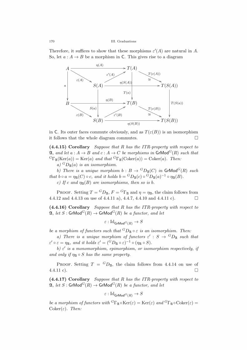
170 III. Graduations
Therefore, it suffices to show that these morphisms ε′(A) are natural in A.
So, let a : A→ B be a morphism in C. This gives rise to a diagram
Aη(A)
//
ε(A) &&MMMMMMMMMMMM
a
T (A)
T (a)
T (ε(A))
∼= ((PPPPPPPPPPPPP
S(A)η(S(A))
//
ε′(A)77oooooooooooo
S(a)
T (S(A))
T (S(a))
Bη(B)
//
ε(B) &&MMMMMMMMMMMM T (B)T (ε(B))
∼= ((PPPPPPPPPPPPP
S(B)η(S(B))
//ε′(B)
77ooooooooooooT (S(B))
in C. Its outer faces commute obviously, and as T (ε(B)) is an isomorphism
it follows that the whole diagram commutes.
(4.4.15) Corollary Suppose that R has the ITR-property with respect to
A, and let a : A→ B and c : A→ C be morphisms in GrModG(R) such thatGΓA(Ker(a)) = Ker(a) and that GΓA(Coker(a)) = Coker(a). Then:
a) GDA(a) is an isomorphism.
b) There is a unique morphism b : B → GDA(C) in GrModG(R) such
that b a = ηA(C) c, and it holds b = GDA(c) GDA(a)−1 ηA(B).
c) If c and ηA(B) are isomorphisms, then so is b.
Proof. Setting T = GDA, F = GΓA and η = ηA, the claim follows from
4.4.12 and 4.4.13 on use of 4.4.11 a), 4.4.7, 4.4.10 and 4.4.11 c).
(4.4.16) Corollary Suppose that R has the ITR-property with respect to
A, let S : GrModG(R)→ GrModG(R) be a functor, and let
ε : IdGrModG(R) → S
be a morphism of functors such that GDA ε is an isomorphism. Then:
a) There is a unique morphism of functors ε′ : S → GDA such that
ε′ ε = ηA, and it holds ε′ = (GDA ε)−1 (ηA S).
b) ε′ is a monomorphism, epimorphism, or isomorphism respectively, if
and only if ηA S has the same property.
Proof. Setting T = GDA, the claim follows from 4.4.14 on use of
4.4.11 c).
(4.4.17) Corollary Suppose that R has the ITR-property with respect to
A, let S : GrModG(R)→ GrModG(R) be a functor, and let
ε : IdGrModG(R) → S
be a morphism of functors with GΓAKer(ε) = Ker(ε) and GΓACoker(ε) =
Coker(ε). Then:
4. Cohomology of graded modules 171
a) GDA ε is an isomorphism.
b) There is a unique morphism of functors ε′ : S → GDA such that
ε′ ε = ηA, and it holds ε′ = (GDA ε)−1 (ηA S).
c) ε′ is a monomorphism, epimorphism, or isomorphism respectively, if
and only if ηA S has the same property, and this is the case if and only ifGΓA S = 0, GH1
A S = 0, or GΓA S = GH1A S = 0 respectively.
Proof. Claim a) holds by 4.4.15, and hence claim b) and the first equiv-
alence in claim c) follow from 4.4.16. The second equivalence in claim c)
can be read off the exact sequence YA S.
4.5. Cech cohomology
Let a = (ai)ni=1 be a finite sequence in Rhom. By a Z-quasigraduation on a
G-graded R-module we always mean a (Z, IdGrModG(R))-quasigraduation.
In this section we introduce graded Cech cohomology, and we investigate
if it coincides with local cohomology; see [2, 5.1] for the ungraded situation
with Noetherian hypotheses. We start by defining the graded Cech cocom-
plex functor.
(4.5.1) For k,m ∈ N0, we denote by I km the set of all strictly increasing
sequences of length k in [1,m] ⊆ Z. For k, s ∈ N0, we denote by ιs ∈ I kk+1
the map defined by
ιs(j) :=
j, if j < s;
j + 1, if j ≥ s.
Then, for m ∈ N0 we have the map ·s : I k+1m → I k
m, f 7→ f s := f ιs, and
for t ∈ N0 it holds
·t ·s =
·s−1 ·t, if s > t;
·s ·t+1, if s ≤ t.
Furthermore, for k ∈ N0 and f ∈ I kn , the map af := a f = (afi)
ki=1 is
a sequence of length k in a1, . . . , an ⊆ Rhom, and therefore we can define∏af =
∏ki=1 afi ∈ Rhom.
(4.5.2) Let M be a G-graded R-module. For k ∈ Z, let
GC(a,M)k :=
⊕f∈I k
nM∏
af , if k ≥ 0;
0, if k < 0.
We denote by GC(a,M) the Z-quasigraded object in GrModG(R) with un-
derlying G-graded R-module⊕
k∈ZGC(a,M)k and with Z-quasigraduation
(GC(a,M)k)k∈Z). We have GC(a,M)0 = M , and for every k ∈ Z \ [0, n] it
holds GC(a,M)k = 0.
For k ∈ Z \ [0, n− 1], let
Gd(a,M)k : GC(a,M)k → GC(a,M)k+1
172 III. Graduations
be the zero morphism. For k ∈ [0, n− 1], f ∈ I kn and g ∈ I k+1
n , the map
Gd(a,M)kf,g : M∏af →M∏
ag
with x 7→ (−1)s−1 agsxags
if f = gs for some s ∈ [1, k + 1] and x 7→ 0 otherwise
is a morphism in GrModG(R), and (Gd(a,M)kf,g)(f,g)∈I kn×I k+1
ninduces a
morphismGd(a,M)k : GC(a,M)k → GC(a,M)k+1
in GrModG(R). Thus, the family (Gd(a,M)k)k∈Z induces a morphism
Gd(a,M) : GC(a,M)→ GC(a,M)(−1)
of Z-quasigraded objects in GrModG(R), and by abuse of language we denote
the pair (GC(a,M),Gd(a,M)) just by GC(a,M).
If ψ : G H is an epimorphism in Ab, then it holds GC(a,M)k[ψ] =HC(a,M[ψ])
k and Gd(a,M)k[ψ] = Hd(a,M[ψ])k for every k ∈ Z, for ψ-
coarsening commutes with modules of fractions and with direct sums by
2.5.3 and 2.1.3. Hence, the pair underlying (GC(a,M),Gd(a,M)) is the
Cech cocomplex of the R-module underlying M with respect to a. This im-
plies that GC(a,M) is a cocomplex in GrModG(R), and we call it the Cech
cocomplex of M with respect to a.
(4.5.3) Let M and N be G-graded R-modules and let h : M → N be a
morphism in GrModG(R). For k ∈ Z \ [0, n], let
GC(a, h)k : GC(a,M)k → GC(a, N)k
be the zero morphism. For k ∈ [0, n] and f ∈ I kn , the map
GC(a, h)kf := h∏af : M∏af → N∏
af
is a morphism in GrModG(R). For k ∈ [0, n], the family (GC(a, h)kf )f∈I kn
induces a morphism
GC(a, h)k : GC(a,M)k → GC(a, N)k
in GrModG(R). Thus, the family (GC(a, h)k)k∈Z induces a morphism
GC(a, h) : GC(a,M)→ GC(a,M)
of Z-quasigraded objects in GrModG(R).
If ψ : G H is an epimorphism in Ab, then it clearly holds GC(a, h)k[ψ] =HC(a, h[ψ])
k for every k ∈ Z. Hence, we see that the morphism of Z-
quasigraded R-modules underlying GC(a, h) is equal to the morphism in
CCo(Mod(R)) induced by h on the Cech cocomplexes. This implies thatGC(a, h) is a morphism in CCo(GrModG(R)).
(4.5.4) By 4.5.2 and 4.5.3, we have a functor
GC(a, •) : GrModG(R)→ CCo(GrModG(R)),
4. Cohomology of graded modules 173
mapping a G-graded R-module M onto its Cech cocomplex with respect to
a. This functor is called the Cech cocomplex functor with respect to a. If
ψ : G H is an epimorphism in Ab, then it holds
GC(a, •)[ψ] = HC(a, •[ψ]).
(4.5.5) Proposition There is an isomorphism of functors
• ⊗R GC(a, R)∼=−→ GC(a, •).
Proof. Let M be a G-graded R-module. For k ∈ [0, n] and f ∈ I kn ,
the R-bilinear map
ϕk,fM : M ×R∏af →M∏
af , (m, r(∏
af)l) 7→ rm
(∏
af)l
induces a morphism
ϕk,fM : M ⊗R R∏af →M∏
af
in GrModG(R) with m ⊗ r(∏
af)l7→ rm
(∏
af)l. This is an isomorphism, since
the map
ψk,fM : M∏af →M ⊗R R∏
af ,m
(∏
af)l7→ m⊗ 1
(∏
af)l
is the inverse of ϕk,fM . Hence,
ϕkM :=⊕f∈I k
n
ϕk,fM : M ⊗R GC(a, R)k → GC(a,M)k
is an isomorphism in GrModG(R). For k ∈ Z \ [0, n], let
ϕkM : M ⊗R GC(a, R)k → GC(a,M)k
be the zero morphism, and let ϕM be the morphism of Z-quasigraded ob-
jects in GrModG(R) induced by the family (ϕkM )k∈Z. Then, it is straight-
forward to verify that ϕM is a morphism and hence an isomorphism in
CCo(GrModG(R)). Moreover it is readily checked that it is natural in M .
(4.5.6) If M is a flat G-graded R-module, then GC(a,M)k is flat for every
k ∈ Z by 4.5.2 and 2.3.9. In particular, GC(a, R)k is flat for every k ∈ Z.
Next, we look at graded Cech cohomology, and we show that it commutes
with coarsening.
(4.5.7) Proposition The sequence (H i(GC(a, •)))i∈Z is an exact δ-func-
tor from GrModG(R) to GrModG(R).
Proof. Let
S : 0 −→ L −→M −→ N −→ 0
and
S′ : 0 −→ L′ −→M ′ −→ N ′ −→ 0
174 III. Graduations
be short exact sequences in GrModG(R) and let (u, v, w) : S → S′ be a
morphism of short exact sequences in GrModG(R). For k ∈ Z, the R-
module GC(a, R)k is flat by 4.5.6. Hence, in CCo(GrModG(R)) we have the
commutative diagram
0 // L⊗R GC(a, R) //
M ⊗R GC(a, R) //
N ⊗R GC(a, R) //
0
0 // L′ ⊗R GC(a, R) // M ′ ⊗R GC(a, R) // N ′ ⊗R GC(a, R) // 0
with exact rows. Each of its rows corresponds to a family of connecting
morphisms, and together with 4.5.5 their naturality yields the claim.
(4.5.8) The δ-functor (H i(GC(a, •)))i∈Z is denoted by (GH i(a, •))i∈Z and
called the Cech cohomology functor with respect to a.
(4.5.9) Proposition Let ψ : G H be an epimorphism in Ab. Then, for
every i ∈ Z it holds
GH i(a, •)[ψ] = HH i(a, •[ψ]).
Proof. This is clear by 4.5.4 and 4.1.2.
Now, we adapt the proof of [2, 5.1.19] to get a condition under which
local cohomology and Cech cohomology coincide.
(4.5.10) Proposition Let b ∈ Rhom and let b := a q (b). Then, there is
an exact sequence
0 −→ GC(a, •b)(−1)ϕ−→ GC(b, •) ψ−→ GC(a, •) −→ 0
of functors such that for every G-graded R-module M and for every k ∈ Zthe sequence
0 −→ GC(a,Mb)k−1 ϕkM−→ GC(b,M)k
ψkM−→ GC(a,M)k −→ 0
in GrModG(R) splits.
Proof. Let M be a G-graded R-module. For k ∈ [1, n + 1] and f ∈I k−1n there is a canonical isomorphism χk,fM : (Mb)
∏af
∼=−→ Mb(∏
af) in
GrModG(R) that is natural in M . Hence, for k ∈ [1, n] there is an isomor-
phism
χkM :=⊕
f∈I k−1n
χk,fM :⊕
f∈I k−1n
(Mb)∏
af
∼=−→⊕
f∈I k−1n
Mb(∏
af)
in GrModG(R) that is also natural in M . Furthermore, we let ϕkM for k ∈Z \ [1, n + 1] and ψkM for k ∈ Z \ [0, n] be zero morphisms, and we set
ϕn+1M := χ
n+1,Id[1,n]
M and ψ0M := IdM . These morphisms in GrModG(R) are
obviously natural in M .
4. Cohomology of graded modules 175
Now, let k ∈ [1, n]. Then, it holds
I kn+1 = f ∈ I k
n+1 | n+ 1 /∈ f([1, k]) q f ∈ I kn+1 | n+ 1 = f(k).
Hence, we have canonical bijections
λk : I kn
∼=−→ f ∈ I kn+1 | n+ 1 /∈ f([1, k])
and
κk : I k−1n
∼=−→ f ∈ I kn+1 | n+ 1 = f(k).
Using these we see that
GC(b,M)k =⊕
f∈I kn+1
M∏af =
( ⊕f∈I k−1
n
M∏aκk(f)
)⊕( ⊕f∈I k
n
M∏aλk(f)
),
and hence we have the canonical injection
ιkM :⊕
f∈I k−1n
Mb(∏
af) ⊕
f∈I kn+1
M∏af
and the canonical projection
ψkM :⊕
f∈I kn+1
M∏af →
⊕f∈I k
n
M∏af .
Both of these are natural in M . Moreover, we get the monomorphism ϕkM :=
ιkM χkM that is also natural in M . Now it is straightforward to check that
the families (ϕkM )k∈Z and (ψkM )k∈Z yield the claim.
(4.5.11) Let a ⊆ R be a finitely generated G-graded ideal, and let a
be a finite, homogeneous generating system of a. It is easy to see thatGH0(a, •) = GΓa(•). As the local cohomology functors with respect to a
are the right derived functors of GΓa by 4.4.3, universality and 4.5.7 yield a
unique morphism of δ-functors
(gia)i∈Z :(GH i
a(•))i∈Z →
(GH i(a, •)
)i∈Z
such that g0a = IdGΓa
.
(4.5.12) Proposition Let a ⊆ R be a finitely generated G-graded ideal,
let a be a finite, homogeneous generating system of a, and suppose that R
has the ITI-property with respect to every finitely generated G-graded ideal
of R. Then, the morphism of δ-functors
(gia)i∈Z :(GH i
a(•))i∈Z →
(GH i(a, •)
)i∈Z
is an isomorphism.
Proof. By [6, 2.2.1] and 4.5.7 it suffices to show that GH i(a, •) is ef-
faceable for every i ∈ N. So, let I be an injective G-graded R-module. We
show the claim by induction on the number n of elements in a = (ai)ni=1. If
n = 0, then it holds GC(a, I) = 0 and hence GH i(a, I) = 0 for every i ∈ Z.
176 III. Graduations
So, let n > 0 and assume the claim to be true for strictly smaller values of n.
We set b := (ai)n−1i=1 and b := 〈b〉R. By 4.5.10, we have an exact sequence
0 −→ GC(b, Ian)(−1) −→ GC(a, I) −→ GC(b, I) −→ 0
in CCo(GrModG(R)) . Hence, for every i ∈ Z we have an exact sequence
GH i−1(b, I)δi−1
−→ GH i−1(b, Ian) −→ GH i(a, I) −→ GH i(b, I)
in GrModG(R). Moreover, our hypothesis implies that GH i(b, I) = 0 for
i > 0 and that GH i−1(b, I) = 0 for i > 1.
In particular, for i > 1 we have GH i−1(b, Ian) ∼= GH i(a, I). Now, con-
sider the exact sequence
S : 0 −→ GΓ〈an〉R(I) −→ I −→ Ian −→ 0
in GrModG(R). As R has the ITI-property with respect to 〈an〉R, this se-
quence splits, and hence Ian is injective. Therefore, the induction hypothesis
implies that GH i(a, I) ∼= GH i−1(b, Ian) = 0 for every i > 1.
Finally, we have to consider the case i = 1. By 4.5.11, the morphism
δ0 : GH0(b, I)→ GH0(b, Ian)
in GrModG(R) equals
GΓb(ηan) : GΓb(I)→ GΓb(Ian),
where ηan : I → Ian denotes the canonical morphism in GrModG(R). There-
fore, it suffices to show that GΓb(η) is an epimorphism. From the coho-
mology sequence of GΓb associated with S we see that this is equivalent toGH1
b (GΓ〈an〉R(I)) = 0. But, as R has the ITI-property with respect to 〈an〉R,
this holds by the induction hypothesis. Thus, the claim is proven.
(4.5.13) From the proof of 4.5.12 it is seen that instead of having the ITI-property
with respect to every finitely generated G-graded ideal it suffices if R has the ITI-
property with respect to 〈ai〉R for every i ∈ [1, n].
Since Cech cohomology commutes with coarsening, the above result gives
a condition for local cohomology to commute with coarsening, different from
the one given in 4.4.4.
(4.5.14) Corollary Let ψ : G H be an epimorphism in Ab, let a ⊆ R be
a finitely generated G-graded ideal, and assume that R and R[ψ] respectively
have the ITI-property with respect to every finitely generated G- and H-
graded ideal. Then, the morphism of δ-functors
(hiR/a,ψ)i∈Z :(GH i
a(•)[ψ]
)i∈Z →
(HH i
a[ψ](•[ψ])
)i∈Z
is an isomorphism.
Proof. Clear from 4.5.12 and 4.5.9 by choosing a finite, homogeneous
system of generators of a.
CHAPTER IV
Toric Schemes
In this last chapter we will put together what was done previously to
obtain the desired theory of toric schemes.
In Section 1, toric schemes will be defined as schemes of the form XM(R)
as studied in Chapter I, where the projective system of monoidsM is defined
by a fan. So, the results from Chapter I immediately give a bunch of results
on the geometry of toric schemes, depending on properties of the base ring.
Moreover, we characterise properness of toric schemes. In contrast to the
results mentioned above this property depends not on the base ring, but on
the fan.
Section 2 contains the first part of our generalisation of Cox’s work [10]
on homogeneous coordinate rings of toric varieties. First, we introduce the
Cox ring associated with a fan. As this is a ring furnished with a graduation
by a finitely generated group, Chapter III provides tools to handle Cox rings
and graded modules over them. Next, we show how Cox rings give rise to
further schemes of the form XM(R) as in Chapter I, called Cox schemes.
So, with every fan Σ are associated a toric scheme, denoted by XΣ(R),
and a Cox scheme, denoted by YΣ(R), and moreover there is a canonical
morphism YΣ(R) → XΣ(R) that is natural in R, and at the end of Section
2 we show that this morphism is an isomorphism if and only if the fan Σ
is full. Therefore, if Σ is full, Cox schemes yield another description of
toric schemes. But also if Σ is not full, then XΣ(R) is isomorphic to a Cox
scheme on use of an appropriate base change – a further reason to prefer
toric schemes over toric varieties.
On use of homogeneous coordinate rings (that is, Cox rings) Cox ex-
plained in [10] how a graded module F over the Cox ring associated with a
fan Σ gives rise to a quasicoherent sheaf F of modules on the toric variety
XΣ(C). Moreover, he showed – if Σ is simplicial – that every quasicoher-
ent sheaf arises like this, and that this correspondence induces a bijection
between graded ideals of a certain restriction of the Cox ring that are satu-
rated with respect to some irrevelvant ideal, and quasicoherent ideals of the
structure sheaf on XΣ(C). Later, in [18] Mustata generalised the first state-
ment to toric varieties defined by an arbitrary fan. Section 3 is devoted to a
generalisation of these results to Cox schemes, and hence to toric schemes.
In Section 4 we treat the foundations of cohomology on toric schemes.
More precisely, we show how sheaf cohomology on toric schemes and graded
local cohomology over Cox rings are related. Our preparations in Chapter
178 IV. Toric Schemes
III allow to prove a statement analogous to the Serre-Grothendieck corre-
spondence for projective schemes.
Altogether, the foundations for the theory of toric schemes presented in
this chapter will hopefully lead to a better understanding of toric schemes
(and, as a special case, toric varieties) and provide a useful basis for future
work.
1. Toric schemes
Let V be an R-vector space of finite dimension, let n := dimR(V ), let N be
a Z-structure on V , and let M := N∗.
1.1. Toric schemes
We start right away by defining the objects of our main interest.
(1.1.1) By I.1.4.3 and I.1.4.4 there is a contravariant functor
TM (•) := Spec(•[M ]) : Ann→ Sch
over Spec, mapping a ring R onto the monoid R-scheme TM (R) called the
M -torus over R.
(1.1.2) Let Σ be an N -fan. Then, by II.4.3.6 this gives rise to an openly im-
mersive projective system Σ∨M of submonoids of M over the lower semilattice
Σ, and then the construction from I.1.4.10 and I.1.4.13 yields a contravariant
functor
XΣ∨M: Ann→ Sch
over Spec that maps a ring R onto an R-scheme
tΣ∨M (R) : XΣ∨M(R)→ Spec(R).
If Σ 6= ∅, then the zero cone 0 is the smallest element of Σ, and hence
XΣ∨M(R) is furnished with a canonical structure of TM (R)-monomodule R-
scheme. If Σ = ∅, then we have XΣ∨M(R) = ∅, and hence also in this case
XΣ∨M(R) is furnished with a canonical structure of TM (R)-monomodule R-
scheme. So, if R is a ring, then the TM (R)-monomodule R-scheme XΣ∨M(R)
(and by abuse of language also its underlying R-scheme and its underlying
scheme) is called the toric scheme over R associated with Σ (and N). If no
confusion can arise we write XΣ and tΣ instead of XΣ∨Mand tΣ∨M .
If σ ∈ Σ, then XΣ∨M ,σdoes depend not on Σ but only on σ and N , and
if τ 4 σ, then ιΣ∨M ,τ,σ : XΣ∨M ,τ→ XΣ∨M ,σ
does also depend not on Σ but
only on σ, τ and N . If no confusion can arise we denote XΣ∨M ,σand ιΣ∨M ,τ,σ
respectively by Xσ and ιτ,σ, and moreover we denote ιΣ∨M ,σ : Xσ → XΣ by
ισ.
If σ ∈ Σ, then ιτ,σ : Xτ → Xσ for every τ 4 σ and ισ : Xσ → XΣ are
open immersion. Moreover, (Xσ)σ∈Σ is a finite affine open covering of XΣ
that has the intersection property.
1. Toric schemes 179
Now, let R be a ring. For σ, τ ∈ Σ with τ 4 σ we consider Xτ (R)
as an open sub-R-scheme of Xσ(R) by means of ιτ,σ(R), and for σ ∈ Σ
we consider Xσ(R) as an open sub-R-scheme of XΣ(R) by means of ισ(R).
Then, (Xσ(R))σ∈Σ is a finite affine open covering of XΣ(R) that has the
intersection property, that is, for all σ, τ ∈ Σ it holds Xσ(R) ∩ Xτ (R) =
Xσ∩τ (R).
(1.1.3) Example If σ is a sharp N -polycone in V , then the morphisms
ισ : Xσ → Xface(σ) and IdXσ are the same, and if R is a ring, then Xσ(R) =
Xface(σ)(R) is called the toric scheme over R associated with σ (and N). In
particular, TM (R) equals the toric scheme X0(R) over R associated with
the zero cone 0 and N .
(1.1.4) Example Let Σ be an N -fan in V , and let R be a ring. By I.1.4.11
it holds XΣ(R) = ∅ if and only if Σ = ∅ or R = 0.
(1.1.5) Example Let Σ be an N -fan in V , and let R be a ring. Then,
tΣ(R) : XΣ(R) → Spec(R) equals IdSpec(R) if and only if R = 0, or if
Σ 6= ∅ and n = 0. Indeed, suppose that tΣ(R) = IdSpec(R) and that Σ 6= ∅.Then, ι0 : TM (R) → Spec(R) is an open immersion and in particular a
monomorphism, and hence the canonical injection ι from R into the Laurent
algebra S in n indeterminates (Xi)i∈I overR is an epimorphism. Considering
the morphism of R-algebras f : S → S with f(Xi) = X−1i for every i ∈ I we
have f ι = IdS ι, hence epimorphy of ι yields Xi = X−1i for every i ∈ I,
and hence R = 0, or I = ∅ and thus n = 0. The converse holds obviously.
The next two examples show that affine and projective spaces are ex-
amples of toric schemes.
(1.1.6) Example Let σ be a full N -regular N -polycone in V , and let E be
an N -regular N -generating set of σ, hence a Z-basis of N . For a ring R we
denote by R[(Ye)e∈E ] the polynomial algebra in the indeterminates (Ye)e∈Eover R. Since the dual basis E∗ of E generates σ∨ we get an isomorphism
N⊕E0
∼=−→ σ∨M and hence an isomorphism
α : Xσ(•)∼=−→ Spec(•[(Ye)e∈E ])
of contravariant functors from Ann to Sch over Spec. Now, let τ 4 σ, and
let F ⊆ E be such that τ = cone(F ). Then, it is easy to see that there is an
isomorphism
αF : Xτ (•)∼=−→ Spec(•[(Ye)e∈E ]∏
e∈E\F Ye)
of contravariant functors from Ann to Sch over Spec such that the diagram
Xσ(•) α // Spec(•[(Ye)e∈E ])
Xτ (•)αF //
ιτ,σ
OO
Spec(•[(Ye)e∈E ]∏e∈E\F Ye
)
Spec η∏e∈E\F Ye
OO
180 IV. Toric Schemes
commutes. In particular, we have Xσ(•) ∼= Vn• .
(1.1.7) Example Let E be a Z-basis of N . We set
F := E ∪ −∑
e∈E e ⊆ N
and σe := cone(F \ e) for e ∈ E. Then, Ω :=⋃e∈F face(σe) is a complete,
N -regular N -fan in V by II.2.2.14. We denote by R[(Zf )f∈F ] the Z-graded
polynomial algebra in the indeterminates (Zf )f∈F over R with respect to
the constant map F → Z with value 1.
If e ∈ F , then it is easy to see that there is an isomorphism
βe : •[(Yf )f∈F\e]∼=−→ •[(Zf )f∈F ](Ze)
of functors from Ann to Ann over IdAnn, and if moreover e′ ∈ F \ e, then
there is an isomorphism
βe′,e : •[(Yf )f∈F\e]Ye′∼=−→ •[(Zf )f∈F ](ZeZe′ )
of functors from Ann to Ann over IdAnn such that the diagram
•[(Yf )f∈F\e]βe //
ηYe′
•[(Zf )f∈F ](Ze)
(ηZeZe′)0
•[(Yf )f∈F\e]Ye′
βe′,e // •[(Zf )f∈F ](ZeZe′ )
commutes. Hence, on use of 1.1.6 and [EGA, II.2.4.1] we get an isomorphism
XΩ(•)∼=−→ Proj(•[(Zf )f∈F ])
of contravariant functors from Ann to Sch over Spec that induces by restric-
tion and coastriction for every e ∈ F and for every ring R an isomorphism
from Xσe(R) onto the open sub-R-scheme D+(Ze) of Proj(R[(Zf )f∈F ]).
In particular, it holds XΩ(•) ∼= Pn• .
(1.1.8) Example Let n = 1, let Σ be an N -fan in V , and let R be a ring.
If Σ is not full, then it holds either Σ = ∅ or Σ = 0, and hence XΣ(R) = ∅or XΣ(R) = TM (R) by 1.1.4 and 1.1.3. If Σ is full, then there is an x ∈ N \0such that it holds either Σ = 0, cone(x) or Σ = 0, cone(x), cone(−x),and hence XΣ(R) ∼= V1
R or XΣ(R) ∼= P1R by 1.1.6 and 1.1.7.
The general results on base changes from Chapter I imply some sort of
“universality” of toric schemes.
(1.1.9) Let Σ be an N -fan in V . If R is a ring, then XΣ : Ann → Sch
induces a contravariant functor XΣ : Alg(R) → Sch/R over Spec, and it
follows from I.1.4.10 that there is a canonical isomorphism
XΣ(R)×R • ∼= XΣ(•)
1. Toric schemes 181
of contravariant functors from Alg(R) to Sch/R over Spec. In particular,
there is a canonical isomorphism
XΣ(Z)× • ∼= XΣ(•)
of contravariant functors from Ann to Sch over Spec.
Now, let R be a ring. If a ⊆ R is an ideal and p : R R/a denotes
the canonical epimorphism in Ann, then XΣ(p) : XΣ(R/a) → XΣ(R) is a
closed immersion by the above, and by means of this we consider XΣ(R/a)
as a closed sub-R-scheme of XΣ(R). If f ∈ R and ηf (R) : R → Rf denotes
the canonical epimorphism, then XΣ(ηf (R)) : XΣ(Rf )→ XΣ(R) is an open
immersion by the above, and by means of this we consider XΣ(Rf ) as an
open sub-R-scheme of XΣ(R).
(1.1.10) Let Σ be an N -fan in V , and let Σ′ ⊆ Σ be a subfan. If R is
a ring, then XΣ′(R) =⋃σ∈Σ′ Xσ(R) ⊆ XΣ(R) is an open sub-R-scheme of
XΣ(R), and hence there is a canonical monomorphism XΣ′ XΣ.
The above base change behaviour of toric schemes gives rise to a tech-
nique of reduction to toric schemes defined by full fans. One should note
that this feature is not available for toric varieties.
(1.1.11) Lemma Let Σ be an N -fan in V , let V ′ := 〈Σ〉, let N ′ := N∩V ′,and let Σ′ denote the set Σ considered as an N ′-fan in V ′. Then, there is
an isomorphism
XΣ(•) ∼= XΣ′(•[N/N ′])
of contravariant functors from Ann to Sch over Spec.
Proof. By 1.1.9 there are canonical isomorphisms
XΣ(•) ∼= XΣ(Z)× •
and
XΣ′(•[N/N ′]) ∼= XΣ′(Z)× (•[N/N ′]) ∼= XΣ′(Z)× (Z[N/N ′])× •
of contravariant functors over Spec, and hence it suffices to show that there
is an isomorphism of schemes XΣ(Z) ∼= XΣ′(Z)× (Z[N/N ′]).
We set M ′ := (N ′)∗, and for σ ∈ Σ we denote by σ′ the set σ consid-
ered as an N ′-polycone in Σ′. As the group M ′ is free, we can choose an
isomorphism M ′ ⊕N/N ′∼=−→M in Ab. If σ ∈ Σ, this induces by restriction
and coastriction an isomorphism (σ′)∨M ′ ⊕ N/N ′∼=−→ σ∨M in Mon such that
for every τ 4 σ the diagram
(σ′)∨M ′ ⊕N/N ′∼= //
_
σ∨M _
(τ ′)∨M ′ ⊕N/N ′
∼= // τ∨M
182 IV. Toric Schemes
in Mon commutes. As the functor Z[•] : Mon→ Ann commutes with coprod-
ucts by I.1.3.1, these isomorphisms induce for every σ ∈ Σ an isomorphism
Z[(σ′)∨M ′ ]⊗ Z[N/N ′]∼=−→ Z[σ∨M ]
in Ann and hence by taking spectra an isomorphism
Xσ(Z)∼=−→ Xσ′(Z)× Spec(Z[N/N ′])
in Sch such that for every τ 4 σ the diagram
Xσ(Z)∼= // Xσ′(Z)× Spec(Z[N/N ′])
Xτ (Z)∼= //
ιτ,σ(Z)
OO
Xτ ′(Z)× Spec(Z[N/N ′])
ιτ ′,σ′ (Z)×IdSpec(Z[N/N′])
OO
in Sch commutes. Thus, these isomorphisms can be glued to obtain an
isomorphism XΣ(Z)∼=−→ XΣ′(Z)× Spec(Z[N/N ′]) in Sch as desired.
(1.1.12) Note that the isomorphism in 1.1.11 depends on the choice of an isomor-
phism M ′ ⊕N/N ′ ∼= M in Ab and is therefore not canonical.
1.2. Basic properties of toric schemes
Let Σ be an N -fan in V , and let R be a ring.
In this section we apply the results from I.2 to describe some fundamental
properties of toric schemes.
(1.2.1) Proposition a) XΣ(R) is separated, quasicompact, flat and of
finite presentation over R.
b) XΣ(R) is faithfully flat over R if and only if Σ 6= ∅ or R = 0.
Proof. This follows from II.4.3.4, I.2.1.2, I.2.2.1, II.4.3.1, I.2.1.3 b) and
I.2.2.2.
(1.2.2) Proposition a) XΣ(R) is reduced, connected or normal, respec-
tivly, if and only if R is so, or Σ = ∅.b) XΣ(R) is irreducible or integral, respectively, if and only if R is so
and Σ 6= ∅.
Proof. This follows from II.4.3.1, I.2.3.8, I.2.4.3 and I.2.5.3.
(1.2.3) Proposition If Σ 6= ∅, then the map p 7→ XΣ(R/p) defines a
bijection from Min(R) onto the set of irreducible components of XΣ(R).
Proof. Clear from II.4.3.1 and I.2.3.12.
(1.2.4) Proposition a) XΣ(R) is Noetherian if and only if R is Noether-
ian, or Σ = ∅.b) XΣ(R) is Artinian if and only if R is Artinian and n = 0, or R = 0,
or Σ = ∅.
1. Toric schemes 183
Proof. This holds by II.4.3.1, I.2.6.4 b), II.4.3.2 and I.2.6.9.
(1.2.5) Proposition a) If Σ 6= ∅, then it holds
dim(R) + n ≤ dim(XΣ(R)) ≤n−1∑i=0
2i + 2n dim(R).
b) If R is Noetherian and Σ 6= ∅, then it holds
dim(R) + n = dim(XΣ(R)).
c) If R is Noetherian, then XΣ(R) is equidimensional if and only if R
is equidimensional, or Σ = ∅.
Proof. For σ ∈ Σ it holds
rk(Diff(σ∨M )) = dim(〈Diff(σ∨M )〉R) = dim(σ∨) = n
by II.1.2.10. So, all the claims follow from II.4.3.1, I.2.6.7 and I.2.6.10.
1.3. Projections of fans and properness of toric schemes
The aim of this section is to characterise toric schemes that are proper
over their base ring. It will turn out that this property can be characterised
by the fan alone. We start by showing how a toric scheme XΣ(R) can be
covered by the toric schemes XΣ/σ(R) associated with projections of Σ along
every cone σ in Σ.
(1.3.1) Let σ and τ be N -polycones in V with σ 4 τ . Then, τ∨M \ σ⊥ is a
prime monoideal of τ∨M . Indeed, for u ∈ τ∨M \σ⊥ and v ∈ τ∨M it holds v+u ∈τ∨M , and for x ∈ σ we have u(x) > 0 and v(x) ≥ 0, hence (u+ v)(x) > 0 and
therefore u + v ∈ τ∨M \ σ⊥. This shows that τ∨M \ σ⊥ is a monoideal of τ∨M ,
and since τ∨M ∩ σ⊥ is obviously a submonoid of τ∨M it is prime.
Moreover, it is easy to see that there is surjective morphism
pσ(τ)∨Mσ→ τ∨M ∩ σ⊥, u 7→ u pσ N
in Mon. Since pσ induces by restriction and coastriction an epimorphism
N Nσ in Ab this morphism is a monomorphism and hence an isomor-
phism.
(1.3.2) Let σ and τ be N -polycones in V with σ 4 τ . Then, by 1.3.1 and
I.1.3.16 we get a morphism
ϑτ,σ := ϑτ∨M ,τ∨M\σ⊥ : •[τ∨M ]→ •[τ∨M ∩ σ⊥]
of functors from Ann to Ann under IdAnn such that ϑτ,σ(R) is surjective and
that
ϑτ,σ(R)(ex) =
ex, if x ∈ σ⊥;
0, if x /∈ σ⊥
for every ring R and every x ∈ σ∨M .
184 IV. Toric Schemes
Moreover, the inverse of the isomorphism defined in 1.3.1 induces an
isomorphism
πτ,σ : •[τ∨M ∩ σ⊥]∼=−→ •[pσ(τ)∨Mσ
]
of functors form Ann to Ann under IdAnn, and composition with ϑτ,σ yields
a morphism
ϑ′τ,σ : •[τ∨M ]→ •[pσ(τ)∨Mσ]
of functors from Ann to Ann under IdAnn such that ϑ′τ,σ(R) is surjective for
every ring R.
For a further N -polycone ω in V with σ 4 ω 4 τ it is readily checked
on use of I.1.3.16 that the diagram
•[τ∨M ]ϑ′τ,σ // •[pσ(τ)∨Mσ
]
•[ω∨M ]ϑ′ω,σ //
OO
OO
•[pσ(ω)∨Mσ]
OO
OO
of functors from Ann to Ann under IdAnn, where the unmarked morphisms
are induced by the canonical injections of τ∨M and τ∨M ∩ σ⊥ into ω∨M and
ω∨M ∩ σ⊥, commutes.
Composing the above morphisms with Spec we get a closed immersion
χτ,σ : Xτ/σ → Xτ of functors from Ann to Sch over Spec such that for every
ω 4 τ with σ 4 ω the diagram
Xτ/σχτ,σ // Xτ
Xω/σχω,σ //
ιω/σ,τ/σ
OO
Xω
ιω,τ
OO
of functors from Ann to Sch over Spec commutes. If R is a ring and no
confusion can arise, then we consider Xτ/σ(R) as a closed sub-R-scheme of
Xτ (R) by means of χτ,σ(R).
(1.3.3) Lemma Let σ, τ and ω be N -polycones in V with σ 4 ω 4 τ .
Then, the diagram
Xτ/σχτ,σ // Xτ
Xω/σχω,σ //
ιω/σ,τ/σ
OO
Xω
ιω,τ
OO
in Hom(Ann, Sch)/Spec is cartesian.
Proof. By II.4.3.3 there is a u ∈ τ∨M ∩ σ⊥ with ω = τ ∩ u⊥ and ω∨M =
τ∨M ⊕N0(−u), and then I.1.2.10 implies ω∨M ∩ σ⊥ = (τ∨M ∩ σ⊥)⊕N0(−u).
1. Toric schemes 185
Now, let R be a ring. It suffices to show that the diagram
R[τ∨M ∩ σ⊥]
ε
R[τ∨M ]ϑτ,σ(R)
oo
R[εu]
R[ω∨M ∩ σ⊥] R[ω∨M ]
ϑω,σ(R)oo
in Alg(R), where ε is induced by restriction and coastriction of εu, is co-
cartesian. By I.1.3.8 we have
A := R[τ∨M ∩ σ⊥]⊗R[τ∨M ] R[ω∨M ] = R[τ∨M ∩ σ⊥]⊗R[τ∨M ] R[τ∨M ⊕N0(−u)] ∼=
R[τ∨M ∩ σ⊥]⊗R[τ∨M ] (R[τ∨M ]⊗R R[N0(−u)]) ∼= R[τ∨M ∩ σ⊥]⊗R R[N0(−u)] ∼=
R[(τ∨M ∩ σ⊥)⊕N0(−u)] = R[ω∨M ∩ σ⊥]
and hence an isomorphism λ : A∼=−→ R[ω∨M∩σ⊥]. Denoting by λ0 and λ1 the
canonical morphisms from R[τ∨M ∩σ⊥] and R[τ∨M⊕N0(−u)] to A it is readily
checked that λλ0ϑτ,σ(R) = εϑτ,σ(R) and λλ1R[εu] = ϑω,σ(R)R[εu].
Since ϑτ,σ(R) and R[εu] are epimorphisms by 1.3.2, I.1.2.2 and I.1.3.13 this
implies λ λ0 = ε and λ λ1 = ϑω,σ(R), and thus the claim.
(1.3.4) Lemma Let σ, τ and ω be N -polycones in V with σ 4 τ and
σ 64 ω 4 τ . If I denotes the initial object in Hom(Ann, Sch)/Spec, then the
diagram
Xτ/σχτ,σ // Xτ
I //
OO
Xω
ιω,τ
OO
in Hom(Ann, Sch)/Spec is cartesian.
Proof. By II.4.3.3 there is a u ∈ τ∨M \ σ⊥ with ω = τ ∩ u⊥ and ω∨M =
τ∨M ⊕N0(−u).
Now, let R be a ring. It suffices to show that the diagram
R[τ∨M ∩ σ⊥]
R[τ∨M ]ϑτ,σ(R)
oo
R[εu]
0 R[τ∨M ⊕N0(−u)]oo
in Alg(R) is cocartesian, and for this it suffices to show that
A := R[τ∨M ∩ σ⊥]⊗R[τ∨M ] R[τ∨M ⊕N0(−u)] = 0,
where R[τ∨M∩σ⊥] is considered as an R[τ∨M ]-algebra by means of ϑτ,σ(R). By
the above we have ϑτ,σ(R)(eu) = 0, and eu ∈ R[τ∨M ⊕N0(−u)] is invertible.
Therefore, for the unit of A we get
1⊗ 1 = 1⊗ (eue−u) = eu(1⊗ e−u) = ϑτ,σ(R)(eu)⊗ e−u = 0,
hence A = 0 and thus the claim.
186 IV. Toric Schemes
(1.3.5) Proposition Let σ be an N -polycone in V , and let R be a ring.
Then, it holds Xσ/σ(R) = Xσ(R) \⋃τ≺σXτ (R).
Proof. By 1.3.4 we have Xσ/σ(R) ⊆ Xσ(R)\⋃τ≺σXτ (R). Conversely,
let p ∈ Xσ(R) \⋃τ≺σXτ (R). Let u ∈ σ∨M \ σ⊥. Then, τ := σ ∩ u⊥
is a face of σ. If eu /∈ p, then we see on use of [AC, II.4.3 Proposition
13, Corollaire], II.4.3.3 and I.1.3.14 that there exists q ∈ Spec(R[σ∨M ]eu) =
Xτ (R) with p = ιτ,σ(R)(q), and then the choice of p implies τ = σ and
hence the contradiction u ∈ σ⊥. So, it holds eu ∈ p, and from this we get
Ker(ϑσ,σ(R)) = 〈eu | u ∈ σ∨M \ σ⊥〉 ⊆ p. But by [AC, II.4.3 Remarque] this
is equivalent to p ∈ Xσ,σ(R), and thus the claim is proven.
(1.3.6) Lemma Let f : Y → X be a morphism in Sch, and let (Xi)i∈I and
(Yj)j∈J respectively be open coverings of X and Y that have the intersection
properties such that J is a segment1 of I. Moreover, suppose that f induces
for every j ∈ J a closed immersion fj : Yj → Xj, and that for all i ∈ I and
all j ∈ J it holds
f−1j (Xinf(i,j)) =
Yinf(i,j), if i ∈ J ;
∅, if i /∈ J.
Then, f is a closed immersion.
Proof. Let i ∈ I, and let gi : f−1(Xi) → Xi denote the morphism
induced by f . By [EGA, I.4.2.4] it suffices to show that gi is a closed
immersion. For every j ∈ J it holds Yj ⊆ f−1(Xj), and the intersection
property implies Yj ∩ f−1(Xi) = Yj ∩ f−1(Xinf(i,j)). Hence, from [EGA,
0.1.2.14] it follows
Yj ∩ f−1(Xi) = Yj ∩ f−1(Xinf(i,j)) = Yj ×X Xinf(i,j) =
Yj ×Xj Xinf(i,j) = f−1j (Xinf(i,j)).
Therefore, we get f−1(Xi) =⋃j∈J f
−1j (Xinf(i,j)). If i ∈ J , it follows
f−1(Xi) =⋃j∈J Yinf(i,j) = Yi ⊆ f−1(Xi),
and hence gi = fi is a closed immersion. If i /∈ J , we have f−1(Xi) = ∅,and then gi is obviously a closed immersion, too. Herewith, the claim is
proven.
(1.3.7) Proposition Let Σ be an N -fan in V , and let σ ∈ Σ. Then, there
exists a unique morphism χσ : XΣ/σ → XΣ of functors from Ann to Sch over
1If E is an ordered set, then a subset F ⊆ E is called a segment of E if for every
x ∈ F it holds E≤x ⊆ F . Note that if E is a lower semilattice and F is a segment of E,
then F is a lower subsemilattice of E, that is, for all x, y ∈ F it holds infE(x, y) ∈ F .
1. Toric schemes 187
Spec such that for every τ ∈ Σσ the diagram
XΣ/σχσ // XΣ
Xτ/σ
ιτ/σ
OO
χτ,σ // Xτ
ιτ
OO
commutes, and χσ : XΣ/σ → XΣ is a closed immersion.
Proof. Existence and uniqueness of χσ are clear by 1.3.2. Let R be a
ring, let τ ∈ Σσ, and let ω ∈ Σ. By 1.3.6 and 1.3.2 it suffices to show that
Xτ/σ(R)×Xτ (R) Xτ∩ω(R) = X(τ∩ω)/σ(R)
if σ 4 ω and that Xτ/σ(R)×Xτ (R)Xτ∩ω(R) = ∅ if σ 64 ω. To do this we can
assume without loss of generality that ω 4 τ , and then the claim follows
from 1.3.3 and 1.3.4.
(1.3.8) Let Σ be an N -fan in V , let σ ∈ Σ, and let R be a ring. If no
confusion can arise, then we consider XΣ/σ(R) as a closed sub-R-scheme of
XΣ(R) by means of χσ(R).
(1.3.9) Corollary Let Σ be an N -fan in V , let σ ∈ Σ, and let R be a ring.
Then, (XΣ/σ(R))σ∈Σ is a closed covering of XΣ(R), and (Xσ/σ(R))σ∈Σ is a
locally closed covering of XΣ(R).
Proof. By 1.3.5 we have
XΣ(R) =⋃σ∈Σ
(Xσ(R)\
⋃τ≺σ
Xτ (R))
=⋃σ∈Σ
Xσ/σ(R) ⊆⋃σ∈Σ
XΣ/σ(R) ⊆ XΣ(R),
and hence the claim follows from 1.3.7.
Now we attack the characterisation of properness by means of the well-
known valuative criterion. As before, base change properties allow reducing
to a Noetherian base ring and hence to discrete valuation rings.
(1.3.10) Lemma Let R be a ring. Then, the following statements are
equivalent:
(i) TM (R) is proper over R;
(ii) VnR is proper over R;
(iii) R = 0 or n = 0.
Proof. On use of the valuative criterion for properness [EGA, II.7.3.8]
and I.1.3.1 it is easily seen that (i) and (ii) respectively holds if and only
if n = 0 or if for every R-algebra A that is a valuation ring2 with field of
fractions K it holds A∗ = K∗ or A = K, respectively. But this is the case if
and only if n = 0 or if there exists no R-algebra A that is a valuation ring.
2We use the terminology of [EGA], that is, a valuation ring is a valuation ring in the
sense of [AC] that is not a field.
188 IV. Toric Schemes
Clearly, this holds ifR = 0. Conversely, ifR 6= 0, then there exists a maximal
ideal m in R by [AC, I.8.6 Theoreme 1], and then the ring of fractions
(R/m)[X]〈X〉 of the polynomial algebra (R/m)[X] in one indeterminate over
R is an R-algebra that is integral, local and Noetherian but not a field, and
its maximal ideal is principal. Therefore, it is a (discrete) valuation ring by
[AC, VI.3.6 Proposition 9], and thus the claim is proven.
(1.3.11) Lemma Let R be a ring, let Σ be a complete N -fan in V , let
α : R → A be an R-algebra such that A is a discrete valuation ring, let
η : A → K be the canonical injection into the field of fractions of A, and
let f : Spec(K) → XΣ(R) be a morphism in Sch/R. Then, there exists a
morphism g : Spec(A)→ XΣ(R) in Sch/R such that g Spec(η) = f .
Proof. By 1.3.9 there is a σ ∈ Σ with f(Spec(K)) ⊆ Xσ/σ(R), and
hence by [EGA, I.4.6.2] there is a morphism f ′ : Spec(K) → Xσ/σ(R) in
Sch/R such that χσ(R)ισ/σ(R)f ′ = f . Then, f ′ corresponds to a morphism
p : R[Mσ]→ K in Alg(R), and by I.1.3.1 this corresponds to a morphism u
in Mon from Mσ to the multiplicative monoid underlying K. Since Mσ is a
group it holds u(Mσ) ⊆ K∗.Now, asK is the field of fractions of the discrete valuation ring A, there is
a valuation v : K → Z∞ of K with ring A, hence, in particular, a morphism
v in Mon from the multiplicative monoid underlying K to Z∞ such that
x ∈ K | v(x) ≥ 0 = A (see [AC, VI.3.6]). Then, coastriction of v u yields
a morphism w : Mσ → Z in Mon, that is, w ∈M∗σ = Nσ.
As Σ/σ is complete by II.2.2.7 c), there is a τ ∈ Σσ with w ∈ τ/σ and
hence (τ/σ)∨Mσ⊆ w∨ ∩Mσ. It follows that for every x ∈ (τ/σ)∨Mσ
we have
v(u(x)) = w(x) ≥ 0 and therefore u(x) ∈ A. Thus, there is a morphism
t from (τ/σ)∨Mσto the multiplicative monoid underlying A such that the
diagram
Mσu // K
(τ/σ)∨Mσ
t //?
OO
A
η
OO
in Mon commutes. By I.1.3.1 we get a morphism q : R[(τ/σ)∨Mσ] → A in
Alg(R) such that the diagram
R[Mσ]p // K
R[(τ/σ)∨Mσ]
q //
OO
A
η
OO
in Alg(R), where the unmarked morphism is induced by the canonical in-
jection (τ/σ)∨Mσ→ Mσ, commutes. Taking spectra yields a morphism
1. Toric schemes 189
g′ : Spec(A)→ Xτ/σ(R) in Sch/R such that the diagram
Spec(K)f ′ //
Spec(η)
Xσ/σ(R)
ισ/σ,τ/σ(R)
Spec(A)
g′ // Xτ/σ(R)
in Sch/R commutes, and then with g := χσ(R) ιτ/σ(R) g′ the claim
holds.
(1.3.12) Theorem Let Σ be an N -fan in V , and let R be a ring. Then,
the following statements are equivalent:
(i) XΣ(R) is proper over R;
(ii) Σ is complete, or Σ = ∅, or R = 0.
Proof. If Σ = ∅ or R = 0 this is clear. So, let Σ 6= ∅ and R 6= 0.
First, suppose that XΣ(R) is proper over R. We show by induction on n
that Σ is complete. If n = 0, then Σ = 0 is complete. If n = 1 and
Σ is not complete, then it holds XΣ(R) = TM (R) or XΣ(R) ∼= V1R by
1.1.8, and then 1.3.10 yields a contradiction. So, let n > 1, and suppose
the claim to be true for strictly smaller values of n. If Σ1 = ∅, then we
have Σ = 0, hence XΣ(R) = TM (R), and therefore 1.3.10 yields again a
contradiction. Thus, it holds Σ1 6= ∅, and then by II.2.3.12 it suffices to show
that Σ/ρ is complete for every ρ ∈ Σ1. So, let ρ ∈ Σ1. By 1.3.7 we have
a closed immersion XΣ/ρ(R) → XΣ(R), and since closed immersions and
compositions of proper morphisms are proper by [EGA, II.5.4.2] it follows
that XΣ/ρ(R) is proper over R and hence Σ/ρ is complete by our hypothesis.
Conversely, suppose that Σ is complete. As Z is Noetherian and tΣ(Z)
is quasicompact and of finite type by 1.2.1 a), the valuative criterion for
properness [EGA, II.7.3.8] and 1.3.11 imply that tΣ(Z) is proper. Since
properness is stable under base change, it follows from 1.1.9 that tΣ(R) is
proper, too.
Combined with the Completion Theorem II.3.7.5 the above implies that
every toric scheme can be openly embedded in a proper toric scheme “in a
toric way”.
(1.3.13) Corollary Let Σ be a (simplicial) N -fan in V . Then, there exists
a (simplicial) N -fan Σ′ in V and an open immersion u : XΣ → XΣ′ such
that XΣ′(R) is proper over R for every ring R.
Proof. Clear by II.3.7.5, 1.1.10 and 1.3.12.
190 IV. Toric Schemes
2. Cox schemes
Let V be an R-vector space of finite dimension, let n := dimR(V ), let N
be a Z-structure on V , let M := N∗, and let Σ be an N -fan in V . If no
confusion can arise, then we set A := AΣ1, a := aΣ1, and c := cΣ1, and if
moreover Σ is full, then we consider Pic(Σ) by means of bΣ as a subgroup
of A.
2.1. Cox rings
We start by introducing some definitions concerning the lower standard
sequence of a fan.
(2.1.1) It holds Diff(NΣ10 ) = ZΣ1 , and by means of the canonical morphism
NΣ10 → ZΣ1 in Mon we consider NΣ1
0 as a submonoid of ZΣ1 . Hence, we
can and do consider every monoid of differences of NΣ10 as a submonoid of
ZΣ1 . If no confusion can arise, then we denote the canonical basis of the
free monoid NΣ10 by (δρ)ρ∈Σ1 .
By means of restriction of a : ZΣ1 → A we consider submonoids of ZΣ1 ,
and in particular monoids of differences of NΣ10 , as monoids over A. We set
a+Σ1
:= a N
Σ10
: NΣ10 → A, and if no confusion can arise we write a+ := a+
Σ1.
For ρ ∈ Σ1 we set αρ := a(δρ) ∈ A.
(2.1.2) For σ ∈ Σ we set
δσ :=∑
ρ∈Σ1\σ1
δρ ∈ NΣ10
and ασ := a(δσ) ∈ A. Then, for cones σ and τ in Σ we have δτ ∈ NΣ10 + δσ
if and only if τ 4 σ, and then it holds
NΣ10 − δτ = (NΣ1
0 − δσ)− (δτ − δσ)
and hence NΣ10 − δσ ⊆ NΣ1
0 − δτ . Furthermore, the canonical injection
NΣ10 − δσ → NΣ1
0 − δτ and the canonical epimorphism
εδτ−δσ : NΣ1
0 − δσ → (NΣ10 − δσ)− (δτ − δσ)
are equal.
The monoideal of NΣ10 generated by δσ | σ ∈ Σ is denoted by IΣ and
called the irrelevant monoideal associated with Σ. Obviously it is generated
by δσ | σ ∈ Σmax.
Now we define the Cox ring associated with a fan (or more precisely, with
the set of its 1-dimensional cones)3. This makes use of the graded version
of algebras of monoids as introduced in III.3.4.2. From the beginning on we
carry out the whole construction relative to a subgroup B of the group A of
degrees. Later on, B will be supposed to fulfil additional conditions (making
3This must not be confused with Cox rings as introduced by Hu and Keel in [15]
(based also on [10]), although there are of course connections between the two notions.
2. Cox schemes 191
it in some way “big enough”), and finally we specialise to B = Pic(Σ) (see
2.2.4 and 3.4.5).
(2.1.3) Let B ⊆ A be a subgroup. Composing the extension functor
•(A) : Ann→ GrAnnA
first with the functor
•[a+] : GrAnnA → GrAnnA
under IdGrAnnA that maps an A-graded ring R onto the A-graded algebra of
NΣ10 over R with respect to a+ (see III.3.4.2) and then with the restriction
functor •(B) : GrAnnA → GrAnnB, yields a functor
SΣ1,B(•) := •(AΣ1)[a+
Σ1](B) : Ann→ GrAnnB
under •(B). Taking components of degree 0 yields a functor
SΣ1,B(•)0 : Ann→ Ann
under IdAnn, and it is easy to see that
SΣ1,B(•)0 = •[Ker(a+)](B) = •[Im(c) ∩NΣ10 ](B).
In caseB = A we write SΣ1 instead of SΣ1,A. Clearly, we have SΣ1,B(•) =
SΣ1(•)(B), and hence the functors SΣ1(•)0 and SΣ1,B(•)0 from Ann to Ann
under IdAnn are equal.
(2.1.4) Let R be a ring. Then, SΣ1(R) is called the Cox ring associated with
Σ1 (and N) over R. Its underlying R-algebra is the polynomial algebra over
R in indeterminates (Zρ)ρ∈Σ1 , and its A-graduation is given by deg(Zρ) = αρfor every ρ ∈ Σ1. If R′ is a further ring and h : R → R′ is a morphism in
Ann, then the morphism SΣ1(h) : SΣ1(R)→ SΣ1(R′) in GrAnnA is given by
Zρ 7→ Zρ for every ρ ∈ Σ1.
Now, let B ⊆ R be a subgroup. Then, SΣ,B(R) is called the B-restricted
Cox ring associated with Σ (and N) over R. Its underlying R-algebra is the
sub-R-algebra of the polynomial algebra over R in indeterminates (Zρ)ρ∈Σ1
generated by the monomials whose degrees lie in B, that is, by TR,Σ,B :=
TR,Σ1 ∩ SΣ,B(R).
(2.1.5) Example Let R be a ring, let k ∈ N, and let Σ be as in II.4.2.2. Then, we
have A = Z2, and SΣ1(R) is the A-graded polynomial algebra R[Z1, Z2, Z3, Z4] over
R with deg(Z1) = (0, 1), deg(Z2) = (1,−k), deg(Z3) = (0, 1) and deg(Z4) = (1, 0).
The next result gives some information on Noetherianity of Cox rings.
(2.1.6) Proposition Let B ⊆ A be a subgroup, and let R be a ring.
a) The R-algebra SΣ1,B(R) is TR,Σ1,B-Noetherian.
b) If the A-graded R-algebra SΣ1(R) is Noetherian, then the B-graded
R-algebra SΣ,B(R) is Noetherian.
192 IV. Toric Schemes
Proof. a) holds by III.3.3.4 a), for it follows from I.1.2.8 and I.2.6.1
that SΣ1(R) is TR,Σ1-Noetherian. b) holds by III.3.3.5.
The property of a Cox ring SΣ1,B(R) to have a component of degree 0
coinciding with R depends only on the fan Σ, as we show next.
(2.1.7) Proposition Let B ⊆ A be a subgroup, and suppose that Σ is full.
Then, the following statements are equivalent:
(i) Σ is skeletal complete;
(ii) SΣ1,B(•)0 = IdAnn;
(iii) There is a ring R 6= 0 with SΣ1,B(R)0 = R.
Proof. By 2.1.3 we can suppose without loss of generality that B = A.
Furthermore, we know from II.4.2.6 that Σ is skeletal complete if and only if
Im(c)∩NΣ10 = 0, that is, if and only if Ker(a+) = 0. Hence, the equivalence
of (i) and (ii) is clear by 2.1.3. So, suppose that there is a ring R with
R 6= 0 such that SΣ1(R)0 = R. Then, the R-module underlying SΣ1(R)0 =
R[Ker(a+)] is free of rank 1, and from this we get Im(c)∩NΣ10 = Ker(a+) = 0
and thus again by II.4.2.6 that Σ is skeletal complete.
(2.1.8) It is seen from its proof and II.4.2.7 that in 2.1.7 we cannot omit the
hypothesis that Σ is full.
(2.1.9) Corollary Let B ⊆ A be a subgroup, let R be a ring, let F be
a Noetherian B-graded SΣ1,B(R)-module, and let α ∈ B. If Σ is skeletal
complete, then the R-module Fα is Noetherian.
Proof. Clear by III.3.3.6 and 2.1.7.
We already know from the general results in Chapters I and III that Cox
rings behave well under base change, but we state this formally for the sake
of reference.
(2.1.10) Proposition Let B ⊆ A be a subgroup, let R be a ring, and let
R′ be an R-algebra. Then, there is a canonical isomorphism
SΣ1,B(•)⊗R R′ ∼= SΣ1,B(• ⊗R R′)
of functors from Alg(R) to GrAlgB(R′) under (• ⊗R R′)(B).
Proof. Clear by III.3.4.4.
We end this section by introducing the irrelevant ideal of a Cox ring.
This ideals will play a role similar to the irrelevant ideal in a positively
graded ring defining a projective scheme.
(2.1.11) Let R be a ring. For σ ∈ Σ we set
Zσ := expR,N
Σ10
(δσ) =∏
ρ∈Σ1\σ1
Zρ ∈ SΣ1(R),
2. Cox schemes 193
and then it holds deg(Zσ) = ασ (see 2.1.2). The A-graded ideal
IΣ(R) := ExpR,N
Σ10
(IΣ) = 〈Zσ | σ ∈ Σ〉SΣ1(R) ⊆ SΣ1(R)
is called the irrelevant ideal associated with Σ (and N) over R. Clearly,
it holds IΣ(R) = 〈Zσ | σ ∈ Σmax〉SΣ1(R), and IΣ(R) is finitely TR,Σ1-
generated.
Now, let B ⊆ A be a subgroup. The B-graded ideal
IΣ,B(R) := IΣ(R) ∩ SΣ,B(R) = IΣ(R)(B) ⊆ SΣ,B(R)
is called the B-restricted irrelevant ideal associated with Σ (and N) over R;
it is finitely TR,Σ,B-generated by III.3.3.4 b) and 2.1.6 a).
2.2. Cox schemes
Our goal in this and the next section is to give another description of
toric schemes. We start by defining a further projective system of monoids
arising from a fan and also the so-called Cox scheme defined by this system.
(2.2.1) The family ((NΣ10 − δσ)∩Ker(a))σ∈Σ defines a projective system of
submonoids of ZΣ1 over the lower semilattice Σ, and this we denote by CΣ.
Let σ, τ ∈ Σ with τ 4 σ, and let u ∈ σ∨M with τ = σ ∩ u⊥. Then,
it clearly holds c(u) ∈ (NΣ10 − δσ) ∩ Ker(a), and moreover the canonical
injection
(NΣ10 − δσ) ∩Ker(a) → (NΣ1
0 − δτ ) ∩Ker(a)
and the canonical morphism
εc(u) : (NΣ10 − δσ) ∩Ker(a)→ ((NΣ1
0 − δσ) ∩Ker(a))− c(u)
are equal. Indeed, there is a family (uρ)ρ∈Σ1 in Z with c(u) =∑
ρ∈Σ1uρδρ,
and it holds uρ = 0 for every ρ ∈ τ1 and uρ > 0 for every ρ ∈ σ1 \ τ1. Hence,
we have
−c(u) =∑
ρ∈Σ1\σ1−uρδρ +
∑ρ∈σ1\τ1 −uρδρ ∈ N
Σ10 − δτ
and
−δτ =∑
ρ∈σ1\τ1(uρ − 1)δρ +∑
ρ∈Σ1\σ1uρδρ − δσ − c(u) ∈ NΣ1
0 − δσ − c(u),
and therefore
(NΣ10 − δσ) ∩Ker(a)− c(u) ⊆ (NΣ1
0 − δτ ) ∩Ker(a) ⊆
(NΣ10 − δσ − c(u)) ∩Ker(a) = (NΣ1
0 − δσ) ∩Ker(a)− c(u).
This proves the claim.
The above and I.1.4.15 imply that the projective system CΣ of sub-
monoids of ZΣ is openly immersive.
194 IV. Toric Schemes
(2.2.2) Keeping in mind 2.2.1 we apply the construction of I.1.4.10 to
the projective system CΣ of submonoids of ZΣ to get in Hom(Ann,Sch) a
morphism
tCΣ: XCΣ
→ Spec,
for every σ ∈ Σ a morphism tCΣ,σ : XCΣ,σ → Spec and an open immersion
ιCΣ,σ : XCΣ,σ → XCΣ, and for all σ, τ ∈ Σ with τ 4 σ an open immersion
ιCΣ,τ,σ : XCΣ,τ → XCΣ,σ such that if R is a ring, then XCΣ(R) is obtained by
glueing the family (XCΣ,σ(R))σ∈Σ of R-schemes along (XCΣ,σ∩τ )(σ,τ)∈Σ2 . If
no confusion can arise, then we set YΣ := XCΣand uΣ := tCΣ
, Yσ := XCΣ,σ,
uσ := tCΣ,σ and κσ := ιCΣ,σ for σ ∈ Σ, and κτ,σ := ιCΣ,τ,σ for σ, τ ∈ Σ with
τ 4 σ.
If R is a ring, then the R-scheme uΣ(R) : YΣ(R) → Spec(R), and by
abuse of language also its underlying scheme YΣ(R), is called the Cox scheme
over R associated with Σ (and N).
Next, we introduce an additional condition on the subgroup B ⊆ A.
(2.2.3) For σ ∈ Σ, we denote by AΣ or, if no confusion can arise by A, the
subgroup of A generated by ασ | σ ∈ Σ.A subgroup B ⊆ A is called Σ-big (in A) or, if no confusion can arise,
big (in A) if it has finite index in A+B, that is, if for every σ ∈ Σ there is
an mσ ∈ N such that mασ ∈ B.
(2.2.4) Example Obviously, AΣ1 is Σ-big in AΣ1 . If Σ is full and simpli-
cial, then II.4.2.9 shows that Pic(Σ) is Σ-big in AΣ1 .
The following description of Cox schemes generalises the description of
projective schemes in [EGA, II.2.3–4].
(2.2.5) Let B ⊆ A be a big subgroup, let σ ∈ Σ, and let m ∈ N be such
that mασ ∈ B. The functor
SΣ1,B(•)Zmσ
: Ann→ GrAnnA
under •(B) and the canonical morphism
ηZmσ
: SΣ1,B(•)→ SΣ1,B(•)Zmσ
in Hom(Ann,GrAnnB)/•(B)
are independent of the choice of m. We denote
them by SΣ1,B(•)σ and ησ, respectively. Composition with the functor of
taking components of degree 0 from GrAnnB to Ann yields a functor
SΣ1,B(•)(σ) := SΣ1,B(•)(Zmσ )
: Ann→ Ann
under IdAnn and a morphism
η(σ) : SΣ1,B(•)0 → SΣ1,B(•)(σ)
in Hom(Ann,Ann)/IdAnn .
It follows from III.2.5.11 that SΣ1,B(•)σ = (SΣ1(•)σ)(B), and moreover
we have SΣ1,B(•)(σ) = SΣ1(•)(σ).
2. Cox schemes 195
(2.2.6) Let B ⊆ A be a big subgroup, let σ, τ ∈ Σ with τ 4 σ, and let
m ∈ N be such that mασ ∈ B and mατ ∈ B. Then, Zmσ divides Zmτ in
SΣ1,B(R) for every ring R, and hence we have a morphism
ηστ : SΣ1,B(•)σ → SΣ1,B(•)τ
in Hom(Ann,GrAnnB)/•(B)
, mapping a ring R onto the canonical morphism
ηZσZτ
(SΣ1(R)) : SΣ1(R)Zσ→ SΣ1(R)
Zτ
in GrAlgA(R) and being independent of the choice of m. Composition with
the functor •0 : GrAnnB → Ann of taking components of degree 0 yields a
morphism
η(σ)(τ) : SΣ1,B(•)(σ) → SΣ1,B(•)(τ)
in Hom(Ann,Ann)/IdAnn .
(2.2.7) Let B ⊆ A be a big subgroup. It follows from I.1.3.14 and 2.2.5
that for every σ ∈ Σ there is a canonical isomorphism
εσ : •[NΣ10 − δσ](B)
∼=−→ SΣ1,B(•)σ
in Hom(Ann,GrAnnB)/•(B)
such that for all σ, τ ∈ Σ with τ 4 σ the diagram
•[NΣ10 − δσ](B)
εσ
∼=//
SΣ1,B(•)σ
ηστ
•[NΣ1
0 − δτ ](B)
ετ
∼=// SΣ1,B(•)τ
in Hom(Ann,GrAnnB)/•(B)
, where the unmarked morphism is induced by the
canonical injection NΣ10 − δσ → NΣ1
0 − δτ , commutes. Taking components
of degree 0 and keeping in mind 2.1.3 we get for every σ ∈ Σ a canonical
isomorphism
ε(σ) : •[(NΣ10 − δσ) ∩Ker(a)]
∼=−→ SΣ1,B(•)(σ)
in Hom(Ann,Ann)/IdAnn such that for all σ, τ ∈ Σ with τ 4 σ the diagram
•[(NΣ10 − δσ) ∩Ker(a)]
ε(σ)
∼=//
SΣ1,B(•)(σ)
η(σ)(τ)
•[(NΣ10 − δτ ) ∩Ker(a)]
ε(τ)
∼=// SΣ1,B(•)(τ)
in Hom(Ann,Ann)/IdAnn , where the unmarked morphism is induced by the
canonical injection (NΣ10 − δσ) ∩Ker(a) → (NΣ1
0 − δτ ) ∩Ker(a), commutes.
(2.2.8) Let B ⊆ A be a big subgroup. If σ ∈ Σ, then by 2.2.7 we can
and do identify uσ : Yσ → Spec with the composition of Spec with the
canonical injection IdAnn(•) → SΣ1,B(•)(σ). It follows that for all σ, τ ∈ Σ
with τ 4 σ the open immersion κτ,σ : Yτ → Yσ is identified with Spec η(σ)(τ) .
196 IV. Toric Schemes
So, for a ring R we obtain the R-scheme YΣ(R) also by glueing the family
(Spec(SΣ1,B(R)(σ)))σ∈Σ of R-schemes along (Spec(SΣ1,B(R)(σ∩τ)))(σ,τ)∈Σ2 ,
and as is also seen by 2.2.5 this construction is independent of the choice of
the big subgroup B ⊆ A.
2.3. Cox schemes and toric schemes
Now we construct a natural morphism from the Cox scheme YΣ(R) to
the toric scheme XΣ(R), and we show that this is an isomorphism if and
only if the fan Σ is full. Together with the base change results given above
this allows us to apply results on Cox schemes to toric schemes and vice
versa.
(2.3.1) The morphism c : M → ZΣ1 induces by restriction and coastriction
for every σ ∈ Σ a surjective morphism
cσ : σ∨M → (NΣ10 − δσ) ∩Ker(a)
in Mon such that for all σ, τ ∈ Σ with τ 4 σ the diagram
σ∨Mcσ //
_
(NΣ10 − δσ) ∩Ker(a)
_
τ∨M
cτ // (NΣ10 − δτ ) ∩Ker(a)
in Mon commutes.
So, by 2.2.7 we have for every σ ∈ Σ a canonical morphism
c′σ : •[σ∨M ]→ SΣ1(•)(σ)
in Hom(Ann,Ann)/IdAnn such that for all σ, τ ∈ Σ with τ 4 σ the diagram
•[σ∨M ]c′σ //
SΣ1(•)(σ)
η(σ)(τ)
•[τ∨M ]
c′σ // SΣ1(•)(τ)
in Hom(Ann,Ann)/IdAnn , where the unmarked morphism is induced by the
canonical injection σ∨M → τ∨M , commutes.
Taking spectra yields for every σ ∈ Σ a canonical morphism γσ :=
Spec(c′σ) : Yσ → Xσ in Hom(Ann,Sch)/ Spec such that for all σ, τ ∈ Σ with
τ 4 σ the diagram
Yσγσ // Xσ
Yτγτ //
Spec(η(σ)(τ)
)
OO
Xτ
ιτ,σ
OO
in Hom(Ann, Sch)/Spec commutes.
Moreover, if σ ∈ Σ, then cσ and hence also c′σ is surjective, and therefore
γσ is a closed immersion.
2. Cox schemes 197
(2.3.2) Proposition There exists a unique morphism
γΣ : YΣ → XΣ
in Hom(Ann, Sch)/ Spec such that for every σ ∈ Σ it holds ισ γσ = γΣ κσ.
Proof. This follows from the construction of YΣ and 2.3.1.
(2.3.3) Proposition The fan Σ is full if and only if γΣ : YΣ → XΣ is an
isomorphism.
Proof. It follows from II.4.2.3 that
Ker(cσ) = M ∩ 〈Σ〉⊥ ∩ σ∨M = M ∩ 〈Σ〉⊥
for every σ ∈ Σ. Therefore, Σ is full if and only if cσ is an isomorphism for
every σ ∈ Σ, hence if and only if c′σ is an isomorphism for every σ ∈ Σ. This
is equivalent to γσ being an isomorphism for every σ ∈ Σ, and this clearly
holds if and only if γΣ is an isomorphism.
(2.3.4) If Σ is full, then by 2.3.3 we can and do identify YΣ and XΣ by
means of the canonical isomorphism γΣ. So, the results on Cox schemes in
this chapter apply to toric schemes associated with full fans.
On the other hand, suppose that Σ is not full. We denote by Σ′ the
set Σ considered as a full fan in 〈Σ〉, and we set N ′ := N ∩ 〈Σ〉. If R is a
ring, then by 1.1.11 and the above we have a (non-canonical) isomorphism
XΣ(R) ∼= XΣ′(R[N/N ′]) = YΣ′(R[N/N ′]) of schemes, and hence the results
on Cox schemes apply to toric schemes associated with nonfull fans after a
suitable base change.
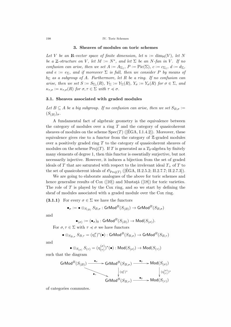
198 IV. Toric Schemes
3. Sheaves of modules on toric schemes
Let V be an R-vector space of finite dimension, let n := dimR(V ), let N
be a Z-structure on V , let M := N∗, and let Σ be an N -fan in V . If no
confusion can arise, then we set A := AΣ1, P := Pic(Σ), c := cΣ1, d := dΣ,
and e := eΣ, and if moreover Σ is full, then we consider P by means of
bΣ as a subgroup of A. Furthermore, let R be a ring. If no confusion can
arise, then we set S := SΣ1(R), YΣ := YΣ(R), Yσ := Yσ(R) for σ ∈ Σ, and
κτ,σ := κτ,σ(R) for σ, τ ∈ Σ with τ 4 σ.
3.1. Sheaves associated with graded modules
Let B ⊆ A be a big subgroup. If no confusion can arise, then we set SB,σ :=
(S(B))σ.
A fundamental fact of algebraic geometry is the equivalence between
the category of modules over a ring T and the category of quasicoherent
sheaves of modules on the scheme Spec(T ) ([EGA, I.1.4.2]). Moreover, these
equivalence gives rise to a functor from the category of Z-graded modules
over a positively graded ring T to the category of quasicoherent sheaves of
modules on the scheme Proj(T ). If T is generated as a T0-algebra by finitely
many elements of degree 1, then this functor is essentially surjective, but not
necessarily injective. However, it induces a bijection from the set of graded
ideals of T that are saturated with respect to the irrelevant ideal T+ of T to
the set of quasicoherent ideals of OProj(T ) ([EGA, II.2.5.2; II.2.7.7; II.2.7.3]).
We are going to elaborate analogues of the above for toric schemes and
hence generalise results of Cox ([10]) and Mustata ([18]) for toric varieties.
The role of T is played by the Cox ring, and so we start by defining the
sheaf of modules associated with a graded module over the Cox ring.
(3.1.1) For every σ ∈ Σ we have the functors
•σ := • ⊗S(B)SB,σ : GrModB(S(B))→ GrModB(SB,σ)
and
•(σ) := (•σ)0 : GrModB(S(B))→ Mod(S(σ)).
For σ, τ ∈ Σ with τ 4 σ we have functors
• ⊗SB,σ SB,τ = (ηστ )∗(•) : GrModB(SB,σ)→ GrModB(SB,τ )
and
• ⊗S(σ)S(τ) = (η
(σ)(τ) )∗(•) : Mod(S(σ))→ Mod(S(τ))
such that the diagram
GrModB(S(B))•σ //
•τ ))SSSSSSSSSSSSSSGrModB(SB,σ)
•0 //
(ηστ )∗
Mod(S(σ))
(η(σ)(τ)
)∗
GrModB(SB,τ )
•0 // Mod(S(τ))
of categories commutes.
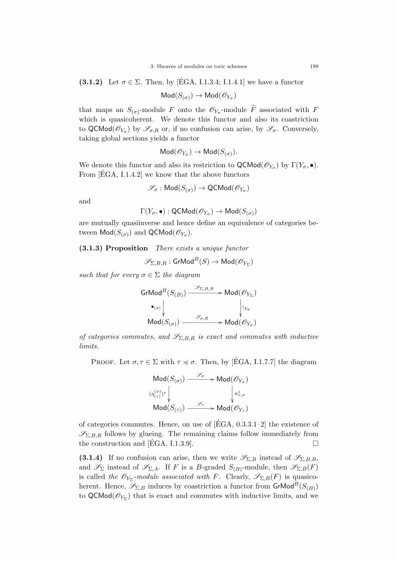
3. Sheaves of modules on toric schemes 199
(3.1.2) Let σ ∈ Σ. Then, by [EGA, I.1.3.4; I.1.4.1] we have a functor
Mod(S(σ))→ Mod(OYσ)
that maps an S(σ)-module F onto the OYσ -module F associated with F
which is quasicoherent. We denote this functor and also its coastriction
to QCMod(OYσ) by Sσ,R or, if no confusion can arise, by Sσ. Conversely,
taking global sections yields a functor
Mod(OYσ)→ Mod(S(σ)).
We denote this functor and also its restriction to QCMod(OYσ) by Γ(Yσ, •).From [EGA, I.1.4.2] we know that the above functors
Sσ : Mod(S(σ))→ QCMod(OYσ)
and
Γ(Yσ, •) : QCMod(OYσ)→ Mod(S(σ))
are mutually quasiinverse and hence define an equivalence of categories be-
tween Mod(S(σ)) and QCMod(OYσ).
(3.1.3) Proposition There exists a unique functor
SΣ,B,R : GrModB(S)→ Mod(OYΣ)
such that for every σ ∈ Σ the diagram
GrModB(S(B))SΣ,B,R //
•(σ)
Mod(OYΣ)
Yσ
Mod(S(σ))Sσ,R // Mod(OYσ)
of categories commutes, and SΣ,B,R is exact and commutes with inductive
limits.
Proof. Let σ, τ ∈ Σ with τ 4 σ. Then, by [EGA, I.1.7.7] the diagram
Mod(S(σ))Sσ //
(η(σ)(τ)
)∗
Mod(OYσ)
κ∗τ,σ
Mod(S(τ))Sτ // Mod(OYτ )
of categories commutes. Hence, on use of [EGA, 0.3.3.1–2] the existence of
SΣ,B,R follows by glueing. The remaining claims follow immediately from
the construction and [EGA, I.1.3.9].
(3.1.4) If no confusion can arise, then we write SΣ,B instead of SΣ,B,R,
and SΣ instead of SΣ,A. If F is a B-graded S(B)-module, then SΣ,B(F )
is called the OYΣ-module associated with F . Clearly, SΣ,B(F ) is quasico-
herent. Hence, SΣ,B induces by coastriction a functor from GrModB(S(B))
to QCMod(OYΣ) that is exact and commutes with inductive limits, and we
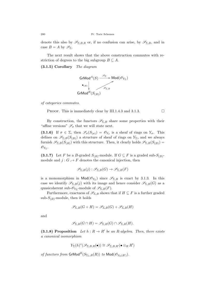
200 IV. Toric Schemes
denote this also by SΣ,B,R or, if no confusion can arise, by SΣ,B, and in
case B = A by SΣ.
The next result shows that the above construction commutes with re-
striction of degrees to the big subgroup B ⊆ A.
(3.1.5) Corollary The diagram
GrModA(S)
•(B)
SΣ // Mod(OYΣ)
GrModB(S(B))
SΣ,B
77oooooooooooo
of categories commutes.
Proof. This is immediately clear by III.1.4.3 and 3.1.3.
By construction, the functors SΣ,B share some properties with their
“affine versions” Sσ that we will state next.
(3.1.6) If σ ∈ Σ, then Sσ(S(σ)) = OYσ is a sheaf of rings on Yσ. This
defines on SΣ,B(S(B)) a structure of sheaf of rings on YΣ, and we always
furnish SΣ,B(S(B)) with this structure. Then, it clearly holds SΣ,B(S(B)) =
OYΣ.
(3.1.7) Let F be a B-graded S(B)-module. If G ⊆ F is a graded sub-S(B)-
module and j : G → F denotes the canonical injection, then
SΣ,B(j) : SΣ,B(G)→ SΣ,B(F )
is a monomorphism in Mod(OYΣ) since SΣ,B is exact by 3.1.3. In this
case we identify SΣ,B(j) with its image and hence consider SΣ,B(G) as a
quasicoherent sub-OYΣ-module of SΣ,B(F ).
Furthermore, exactness of SΣ,B shows that if H ⊆ F is a further graded
sub-S(B)-module, then it holds
SΣ,B(G+H) = SΣ,B(G) + SΣ,B(H)
and
SΣ,B(G ∩H) = SΣ,B(G) ∩SΣ,B(H).
(3.1.8) Proposition Let h : R → R′ be an R-algebra. Then, there exists
a canonical isomorphism
YΣ(h)∗(SΣ,B,R(•)) ∼= SΣ,B,R′(• ⊗R R′)
of functors from GrModB(SΣ1,B(R)) to Mod(OYΣ(R′)).
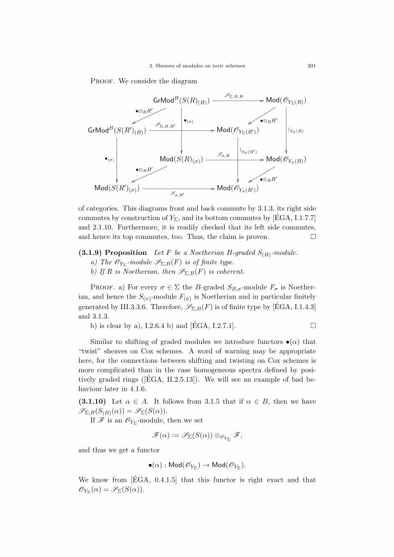
3. Sheaves of modules on toric schemes 201
Proof. We consider the diagram
GrModB(S(R)(B))SΣ,B,R //
•(σ)
•⊗RR′
vvnnnnnnnnnnnnMod(OYΣ(R))
Yσ(R)
•⊗RR′yyssssssssss
GrModB(S(R′)(B))SΣ,B,R′ //
•(σ)
Mod(OYΣ(R′))
Yσ(R′)
Mod(S(R)(σ))Sσ,R //
•⊗RR′
vvmmmmmmmmmmmmMod(OYσ(R))
•⊗RR′yyrrrrrrrrrr
Mod(S(R′)(σ))Sσ,R′
// Mod(OYσ(R′))
of categories. This diagrams front and back commute by 3.1.3, its right side
commutes by construction of YΣ, and its bottom commutes by [EGA, I.1.7.7]
and 2.1.10. Furthermore, it is readily checked that its left side commutes,
and hence its top commutes, too. Thus, the claim is proven.
(3.1.9) Proposition Let F be a Noetherian B-graded S(B)-module.
a) The OYΣ-module SΣ,B(F ) is of finite type.
b) If R is Noetherian, then SΣ,B(F ) is coherent.
Proof. a) For every σ ∈ Σ the B-graded SB,σ-module Fσ is Noether-
ian, and hence the S(σ)-module F(σ) is Noetherian and in particular finitely
generated by III.3.3.6. Therefore, SΣ,B(F ) is of finite type by [EGA, I.1.4.3]
and 3.1.3.
b) is clear by a), I.2.6.4 b) and [EGA, I.2.7.1].
Similar to shifting of graded modules we introduce functors •(α) that
“twist” sheaves on Cox schemes. A word of warning may be appropriate
here, for the connections between shifting and twisting on Cox schemes is
more complicated than in the case homogeneous spectra defined by posi-
tively graded rings ([EGA, II.2.5.13]). We will see an example of bad be-
haviour later in 4.1.6.
(3.1.10) Let α ∈ A. It follows from 3.1.5 that if α ∈ B, then we have
SΣ,B(S(B)(α)) = SΣ(S(α)).
If F is an OYΣ-module, then we set
F (α) := SΣ(S(α))⊗OYΣF ,
and thus we get a functor
•(α) : Mod(OYΣ)→ Mod(OYΣ
).
We know from [EGA, 0.4.1.5] that this functor is right exact and that
OYΣ(α) = SΣ(S(α)).
202 IV. Toric Schemes
(3.1.11) Proposition Suppose that Σ is full, let σ ∈ Σ, and let α ∈ P .
Then, there exists a unique virtual polytope p = (mτ + τ∨)τ∈Σ over Σ such
that mτ = 0 for every τ ∈ face(σ) and that e(p) = α, and the S(σ)-module
S(α)(σ) is free of rank 1 with basis∏ρ∈Σ1
ZρN (mρ)ρ .
Proof. Existence of a unique p with the required properties holds by
II.4.1.9. Furthermore, we have
d(p) =∑ρ∈Σ1
ρN (mρ)δρ ∈ (NΣ10 − δσ) ∩ c−1(α),
and hence there exists for every q ∈ (NΣ10 − δσ) ∩ c−1(α) an m ∈ M with
q = c(m) + d(p), that is, with∏ρ∈Σ1
Zqρρ = (
∏ρ∈Σ1
ZρN (m)ρ )(
∏ρ∈Σ1
ZρN (mρ)ρ )
in Sσ. Since every element of S(α)(σ) = (Sσ)α is an S(σ)-linear combination
of elements of the form∏ρ∈Σ1
Zqρρ with q ∈ (NΣ1
0 − δσ)∩c−1(α), this implies
that∏ρ∈Σ1
ZρN (mρ)ρ generates the S(σ)-module S(α)σ. As this element is
obviously free over S(σ) the claim is proven.
(3.1.12) Corollary Suppose that Σ is full, and let α ∈ P . Then, the
OYΣ-module OYΣ
(α) is invertible.
Proof. Clear from 3.1.11, since OYΣ(α) Yσ= Sσ(S(α)(σ)) for every
σ ∈ Σ.
(3.1.13) Corollary Suppose that Σ is full, let σ ∈ Σ, and let α, β ∈ P .
Then, the morphism
S(α)(σ) ⊗S(σ)S(β)(σ) → S(α+ β)(σ)
in Mod(S(σ)) induced by multiplication of Sσ is an isomorphism.
Proof. The morphism in question is induced by restriction and coas-
triction of the canonical isomorphism Sσ ⊗Sσ Sσ → Sσ and hence injective.
By 3.1.11 there are virtual polytopes p = (mτ +τ∨)τ∈Σ and q = (lτ +τ∨)τ∈Σ
over Σ such that eΣ(p) = α and eΣ(q) = β, and that mτ = 0 and lτ = 0 for
every τ ∈ face(σ). This implies p+ q = (mτ + lτ + τ∨)τ∈Σ and eΣ(p+ q) =
α+ β, and then the claim follows easily on use of 3.1.11.
Now we can show that some rings of fractions of the P -restriction of S
are strongly graded (see III.3.1).
(3.1.14) Corollary Suppose that Σ is full and simplicial, and let σ ∈ Σ.
Then, the P -graded ring SP,σ is strongly graded.
Proof. Since Σ is full and simplicial, the subgroup P ⊆ A is big by
2.2.4. For every α ∈ P the morphism
(Sσ)α ⊗S(σ)(Sσ)−α → S(σ)
3. Sheaves of modules on toric schemes 203
in Mod(S(σ)) induced by multiplication of Sσ is an isomorphism by 3.1.13,
and thus the claim follows from III.3.1.3.
(3.1.15) Corollary Suppose that Σ is full and simplicial, let F be a P -
graded S(P )-module, let σ ∈ Σ, and let α ∈ P . Then, there is an isomor-
phism (Fσ)α ∼= F(σ) in Mod(S(σ)).
Proof. On use of III.2.5.11 we get (SP,σ)β = ((Sσ)(P ))β = (Sσ)β for
every β ∈ P . If we apply this with β = α and β = 0 and keep in mind
3.1.11, then we get an isomorphism (SP,σ)α ∼= S(σ) in Mod(S(σ)). Moreover,
it follows from 3.1.14 and III.3.1.3 that Fσ ∼= SP,σ ⊗S(σ)F(σ) in Mod(S(σ)).
Thus, taking components of degree α yields
(Fσ)α ∼= (SP,σ ⊗S(σ)F(σ))α = (Sσ)α ⊗S(σ)
F(σ)∼= S(σ) ⊗S(σ)
F(σ)∼= F(σ)
in Mod(S(σ)) and hence the claim.
From the above results we derive now quickly a flatness criterion for
sheaves of the form SΣ,B(F ) in terms of the graded module F . In order to
characterise flatness of such sheaves in 3.1.17 we have to suppose that Σ is
simplicial and that B = P .
(3.1.16) Proposition Let F be a B-graded S(B)-module.
a) SΣ,B(F ) is flat over R if and only if F(σ) is flat over R for every
σ ∈ Σ.
b) If Fσ is flat over R for every σ ∈ Σ, then SΣ,B(F ) is flat over R.
Proof. Clearly, SΣ,B(F ) is flat over R if and only if Sσ(F(σ)) =
SΣ,B(F ) Yσ is flat over R for every σ ∈ Σ. By [EGA, IV.2.1.2] this is
the case if and only if F(σ) is flat over R for every σ ∈ Σ, and thus a) is
proven. Now, b) follows from a) and [AC, I.2.3 Proposition 2].
(3.1.17) Corollary Suppose that Σ is full and simplicial, and let F be a
P -graded S(P )-module. Then, SΣ,P (F ) is flat over R if and only if Fσ is
flat over R for every σ ∈ Σ.
Proof. Suppose that SΣ,P (F ) is flat over R. Then, 3.1.16 a) implies
that F(σ) is flat over R for every σ ∈ Σ. Moreover, by 3.1.15 we have
(Fσ)α ∼= F(σ) in Mod(S(σ)) for every σ ∈ Σ and every α ∈ P , and hence (Fσ)αis flat over R for every σ ∈ Σ and every α ∈ P . Thus, Fσ =
⊕α∈P (Fσ)α
is flat over R by [AC, I.2.3 Proposition 2], and together with 3.1.16 b) the
claim is proven.
(3.1.18) We denote by JΣ,B(R) the set of graded ideals of S(B), and we
denote by JΣ(R) the set of quasicoherent ideals of OYΣ. On use of 3.1.6 and
3.1.7 we get a map
ΞΣ,B,R : JΣ,B(R)→ JΣ(R), a 7→ SΣ,B(a),
204 IV. Toric Schemes
and by 3.1.5 it is clear that the diagram
JΣ,A(R)
ΞΣ,A,R // JΣ(R)
JΣ,B(R)
ΞΣ,B,R
88ppppppppppp
in Ens, where the unmarked morphism is induced by the functor •(B), com-
mutes.
If no confusion can arise, then we set JΣ,B := JΣ,B(R), JΣ := JΣ(R),
and ΞΣ,B := ΞΣ,B,R.
3.2. The first total functor of sections
This section is devoted to the preparations for proving that the functors
SΣ,B are essentially surjective. Keeping in mind the proof of the analogous
statement for projective schemes (see [EGA, II.2.7.7]) we start by intro-
ducing a “total functor of sections”. Since shifting and twisting are not
necessarily compatible, there are two possibilities of defining such a functor.
We consider only the first one here, resulting in the first total functor of
sections. The second one – and the connections between the first and the
second one – are studied later in Section 4.1.
We start with a construction that generalises [EGA, 0.5.4.6].
(3.2.1) Let (X,OX) be a ringed space, let G be a group, and let
E =((Eg)g∈G, (µg,h)(g,h)∈G2
)be a couple consisting of a family (Eg)g∈G of OX -modules with E0 = OX and
of a family (µg,h : Eg ⊗OX Eh → Eg+h)(g,h)∈G2 of morphisms in Mod(OX).
Furthermore, we suppose that for all g, h ∈ G it holds µg,h = µh,g σg,h,
where σg,h : Eg⊗OX Eh∼=−→ Eh⊗OX Eg denotes the canonical isomorphism in
Mod(OX), and that for all g, h, k ∈ G it holds
µg+h,k (µg,h ⊗OX IdEk) = µg,h+k (IdEg ⊗OX µh,k).
Let U ⊆ X be an open subset. We consider the G-graded OX(U)(G)-
module⊕
g∈G Γ(U,Eg). For g, h ∈ G we have a canonical morphism
Eg(U)⊗OX(U) Eh(U)→ (Eg ⊗OX Eh)(U),
and it is readily checked that its composition with
µg,h(U) : (Eg ⊗OX Eh)(U)→ Eg+h(U)
yields a structure of G-graded OX(U)(G)-algebra on⊕
g∈G Γ(U,Eg). This G-
graded OX(U)(G)-algebra is denoted by ΓE,U∗ . For every open subset V ⊆ Uthe restriction morphisms Eg(U) → Eg(V ) for g ∈ G induce a morphism
ΓE,U∗ → ΓE,V∗ of G-graded OX(U)(G)-algebras, by abuse of language called
the restriction morphism and denoted by V .
3. Sheaves of modules on toric schemes 205
(3.2.2) We keep the hypotheses of 3.2.1. Let F be an OX -module. We
consider the G-graded OX(U)(G)-module⊕
g∈G Γ(U,Eg ⊗OX F ). For g, h ∈G we have a canonical morphism
Eg(U)⊗OX(U) (Eh ⊗OX F )(U)→ (Eg ⊗OX Eh ⊗OX F )(U),
and it is readily checked that its composition with
(µg,h ⊗OX IdF )(U) : (Eg ⊗OX Eh ⊗OX F )(U)→ (Eg+h ⊗OX F )(U)
yields a structure of G-graded ΓE,U∗ -module on⊕
g∈G Γ(U,Eg⊗OX F ). This
G-graded ΓE,U∗ -module is denoted by ΓE,U∗ (F ). The above gives rise to a
functor
ΓE,U∗ (•) : Mod(OX)→ GrModG(ΓE,U∗ ).
For every open subset V ⊆ U the restriction morphisms
(Eg ⊗OX F )(U)→ (Eg ⊗OX F )(V )
for g ∈ G induce a morphism ΓE,U∗ (F ) → ΓE,V∗ (F ) of G-graded ΓE,U∗ -
modules, by abuse of language called the restriction morphism and denoted
by V . The above gives rise to a morphism
ΓE,U∗ → ΓE,V∗
in Hom(Mod(OX),GrModG(ΓE,U∗ )), by abuse of language also called the re-
striction morphism and denoted by V .
The G-graded ΓE,U∗ -module underlying ΓE,U∗ is ΓE,U∗ (OX). If no confu-
sion can arise, then we denote the G-graded OX(U)(G)-algebra ΓE,U∗ also by
ΓE,U∗ (OX).
Now we apply the above to Cox rings and Cox schemes to get the first
total functor of sections.
(3.2.3) Let α, β ∈ A. For every σ ∈ Σ, multiplication of S defines a
monomorphism
(Sσ)α ⊗S(σ)(Sσ)β → (Sσ)α+β
in Mod(S(σ)) such that for all σ, τ ∈ Σ with τ 4 σ the diagram
(Sσ)α ⊗S(σ)(Sσ)β //
(ηστ )α⊗(ηστ )β
(Sσ)α+β
(ηστ )α+β
(Sτ )α ⊗S(τ)
(Sτ )β // (Sτ )α+β
in Mod(S(σ)) commutes. Hence, by 3.1.2 and 3.1.3 we have for every σ ∈ Σ
a monomorphism
OYΣ(α)(Yσ)⊗OYΣ
(Yσ) OYΣ(β)(Yσ)→ OYΣ
(α+ β)(Yσ)
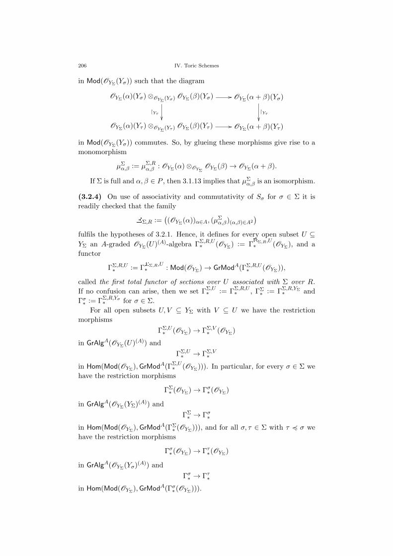
206 IV. Toric Schemes
in Mod(OYΣ(Yσ)) such that the diagram
OYΣ(α)(Yσ)⊗OYΣ
(Yσ) OYΣ(β)(Yσ) //
Yτ
OYΣ(α+ β)(Yσ)
Yτ
OYΣ(α)(Yτ )⊗OYΣ
(Yτ ) OYΣ(β)(Yτ ) // OYΣ
(α+ β)(Yτ )
in Mod(OYΣ(Yσ)) commutes. So, by glueing these morphisms give rise to a
monomorphism
µΣα,β := µΣ,R
α,β : OYΣ(α)⊗OYΣ
OYΣ(β)→ OYΣ
(α+ β).
If Σ is full and α, β ∈ P , then 3.1.13 implies that µΣα,β is an isomorphism.
(3.2.4) On use of associativity and commutativity of Sσ for σ ∈ Σ it is
readily checked that the family
EΣ,R :=((OYΣ
(α))α∈A, (µΣα,β)(α,β)∈A2
)fulfils the hypotheses of 3.2.1. Hence, it defines for every open subset U ⊆YΣ an A-graded OYΣ
(U)(A)-algebra ΓΣ,R,U∗ (OYΣ
) := ΓEΣ,R,U∗ (OYΣ
), and a
functor
ΓΣ,R,U∗ := Γ
EΣ,R,U∗ : Mod(OYΣ
)→ GrModA(ΓΣ,R,U∗ (OYΣ
)),
called the first total functor of sections over U associated with Σ over R.
If no confusion can arise, then we set ΓΣ,U∗ := ΓΣ,R,U
∗ , ΓΣ∗ := ΓΣ,R,YΣ
∗ and
Γσ∗ := ΓΣ,R,Yσ∗ for σ ∈ Σ.
For all open subsets U, V ⊆ YΣ with V ⊆ U we have the restriction
morphisms
ΓΣ,U∗ (OYΣ
)→ ΓΣ,V∗ (OYΣ
)
in GrAlgA(OYΣ(U)(A)) and
ΓΣ,U∗ → ΓΣ,V
∗
in Hom(Mod(OYΣ),GrModA(ΓΣ,U
∗ (OYΣ))). In particular, for every σ ∈ Σ we
have the restriction morphisms
ΓΣ∗ (OYΣ
)→ Γσ∗ (OYΣ)
in GrAlgA(OYΣ(YΣ)(A)) and
ΓΣ∗ → Γσ∗
in Hom(Mod(OYΣ),GrModA(ΓΣ
∗ (OYΣ))), and for all σ, τ ∈ Σ with τ 4 σ we
have the restriction morphisms
Γσ∗ (OYΣ)→ Γτ∗(OYΣ
)
in GrAlgA(OYΣ(Yσ)(A)) and
Γσ∗ → Γτ∗
in Hom(Mod(OYΣ),GrModA(Γσ∗ (OYΣ
))).
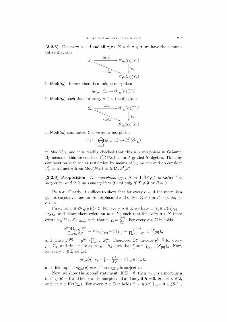
3. Sheaves of modules on toric schemes 207
(3.2.5) For every α ∈ A and all σ, τ ∈ Σ with τ 4 σ, we have the commu-
tative diagram
Sα(ησ)α //
(ητ )α ((RRRRRRRRRRRRRRR OYΣ(α)(Yσ)
Yτ
OYΣ(α)(Yτ )
in Mod(S0). Hence, there is a unique morphism
ηΣ,α : Sα → OYΣ(α)(YΣ)
in Mod(S0) such that for every σ ∈ Σ the diagram
SαηΣ,α //
(ησ)α ((RRRRRRRRRRRRRRRR OYΣ(α)(YΣ)
Yσ
OYΣ(α)(Yσ)
in Mod(S0) commutes. So, we get a morphism
ηΣ :=⊕α∈A
ηΣ,α : S → ΓΣ∗ (OYΣ
)
in Mod(S0), and it is readily checked that this is a morphism in GrAnnA.
By means of this we consider ΓΣ∗ (OYΣ
) as an A-graded S-algebra. Thus, by
composition with scalar restriction by means of ηΣ we can and do consider
ΓΣ∗ as a functor from Mod(OYΣ
) to GrModA(S).
(3.2.6) Proposition The morphism ηΣ : S → ΓΣ∗ (OYΣ
) in GrAnnA is
surjective, and it is an isomorphism if and only if Σ 6= ∅ or R = 0.
Proof. Clearly, it suffices to show that for every α ∈ A the morphism
ηΣ,α is surjective, and an isomorphism if and only if Σ 6= ∅ or R = 0. So, let
α ∈ A.
First, let x ∈ OYΣ(α)(YΣ). For every σ ∈ Σ we have x Yσ∈ S(α)(σ) =
(Sσ)α, and hence there exists an m ∈ N0 such that for every σ ∈ Σ there
exists a y(σ) ∈ Sα+mασ such that xYσ= y(σ)
Zmσ. For every σ ∈ Σ it holds
y(σ)·∏ρ∈σ1
Zmρ∏ρ∈Σ1
Zmρ= xYσY0= xY0=
y(0)∏ρ∈Σ1
Zmρ∈ (S0)α
and hence y(0) = y(σ) ·∏ρ∈σ1
Zmρ . Therefore, Zmρ divides y(0) for every
ρ ∈ Σ1, and thus there exists y ∈ Sα such that y1 = x Y0∈ (S0)α. Now,
for every σ ∈ Σ we get
ηΣ,α(y)Yσ= y1 = y(σ)
Zmσ= xYσ∈ (Sσ)α,
and this implies ηΣ,α(y) = x. Thus, ηΣ,α is surjective.
Now, we show the second statement. If Σ = ∅, then ηΣ,α is a morphism
of rings R→ 0 and hence an isomorphism if and only if R = 0. So, let Σ 6= ∅,and let x ∈ Ker(ηα). For every σ ∈ Σ it holds x
1 = ηα(x) Yσ= 0 ∈ (Sσ)α,
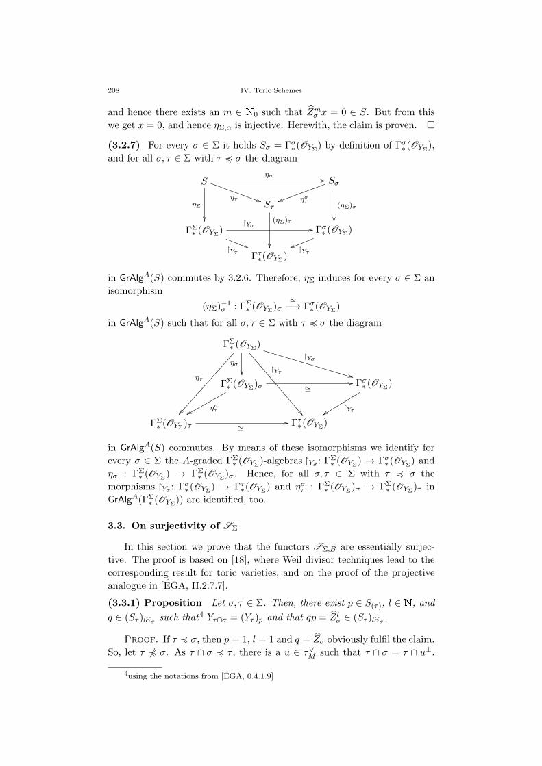
208 IV. Toric Schemes
and hence there exists an m ∈ N0 such that Zmσ x = 0 ∈ S. But from this
we get x = 0, and hence ηΣ,α is injective. Herewith, the claim is proven.
(3.2.7) For every σ ∈ Σ it holds Sσ = Γσ∗ (OYΣ) by definition of Γσ∗ (OYΣ
),
and for all σ, τ ∈ Σ with τ 4 σ the diagram
Sησ //
ητ ))SSSSSSSSSSSS
ηΣ
Sσ
(ηΣ)σ
ηστuukkkkkkkkkkkk
Sτ
(ηΣ)τ
ΓΣ∗ (OYΣ
)Yσ //
Yτ))RRRRRR
Γσ∗ (OYΣ)
Yτvvllllll
Γτ∗(OYΣ)
in GrAlgA(S) commutes by 3.2.6. Therefore, ηΣ induces for every σ ∈ Σ an
isomorphism
(ηΣ)−1σ : ΓΣ
∗ (OYΣ)σ
∼=−→ Γσ∗ (OYΣ)
in GrAlgA(S) such that for all σ, τ ∈ Σ with τ 4 σ the diagram
ΓΣ∗ (OYΣ
)
ησ
ητ
Yτ
::::::::::::::::::Yσ
**UUUUUUUUUUUUUUUUUUUUU
ΓΣ∗ (OYΣ
)σ ∼=//
ηστxxqqqqqqqqqqΓσ∗ (OYΣ
)
Yτyyssssssssss
ΓΣ∗ (OYΣ
)τ ∼=// Γτ∗(OYΣ
)
in GrAlgA(S) commutes. By means of these isomorphisms we identify for
every σ ∈ Σ the A-graded ΓΣ∗ (OYΣ
)-algebras Yσ : ΓΣ∗ (OYΣ
) → Γσ∗ (OYΣ) and
ησ : ΓΣ∗ (OYΣ
) → ΓΣ∗ (OYΣ
)σ. Hence, for all σ, τ ∈ Σ with τ 4 σ the
morphisms Yτ : Γσ∗ (OYΣ) → Γτ∗(OYΣ
) and ηστ : ΓΣ∗ (OYΣ
)σ → ΓΣ∗ (OYΣ
)τ in
GrAlgA(ΓΣ∗ (OYΣ
)) are identified, too.
3.3. On surjectivity of SΣ
In this section we prove that the functors SΣ,B are essentially surjec-
tive. The proof is based on [18], where Weil divisor techniques lead to the
corresponding result for toric varieties, and on the proof of the projective
analogue in [EGA, II.2.7.7].
(3.3.1) Proposition Let σ, τ ∈ Σ. Then, there exist p ∈ S(τ), l ∈ N, and
q ∈ (Sτ )lασ such that4 Yτ∩σ = (Yτ )p and that qp = Z lσ ∈ (Sτ )lασ .
Proof. If τ 4 σ, then p = 1, l = 1 and q = Zσ obviously fulfil the claim.
So, let τ 64 σ. As τ ∩ σ 4 τ , there is a u ∈ τ∨M such that τ ∩ σ = τ ∩ u⊥.
4using the notations from [EGA, 0.4.1.9]
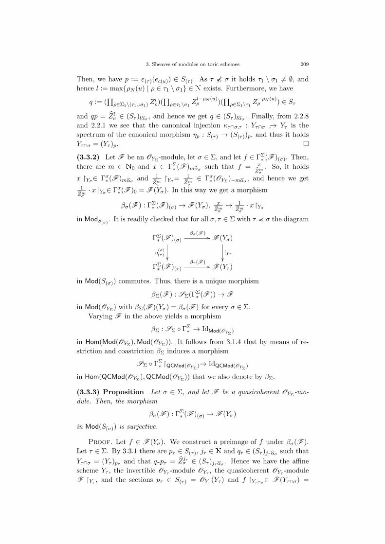
3. Sheaves of modules on toric schemes 209
Then, we have p := ε(τ)(ec(u)) ∈ S(τ). As τ 64 σ it holds τ1 \ σ1 6= ∅, and
hence l := maxρN (u) | ρ ∈ τ1 \ σ1 ∈ N exists. Furthermore, we have
q := (∏ρ∈Σ1\(τ1∪σ1) Z
lρ)(∏ρ∈τ1\σ1
Zl−ρN (u)ρ )(
∏ρ∈Σ1\τ1 Z
−ρN (u)ρ ) ∈ Sτ
and qp = Z lσ ∈ (Sτ )lασ , and hence we get q ∈ (Sτ )lασ . Finally, from 2.2.8
and 2.2.1 we see that the canonical injection κτ∩σ,τ : Yτ∩σ → Yτ is the
spectrum of the canonical morphism ηp : S(τ) → (S(τ))p, and thus it holds
Yτ∩σ = (Yτ )p.
(3.3.2) Let F be an OYΣ-module, let σ ∈ Σ, and let f ∈ ΓΣ
∗ (F )(σ). Then,
there are m ∈ N0 and x ∈ ΓΣ∗ (F )mασ such that f = x
Zmσ. So, it holds
x Yσ∈ Γσ∗ (F )mασ and 1
ZmσYσ= 1
Zmσ∈ Γσ∗ (OYΣ
)−mασ , and hence we get
1
Zmσ· xYσ∈ Γσ∗ (F )0 = F (Yσ). In this way we get a morphism
βσ(F ) : ΓΣ∗ (F )(σ) → F (Yσ), x
Zmσ7→ 1
Zmσ· xYσ
in ModS(σ). It is readily checked that for all σ, τ ∈ Σ with τ 4 σ the diagram
ΓΣ∗ (F )(σ)
βσ(F )//
η(σ)(τ)
F (Yσ)
Yτ
ΓΣ∗ (F )(τ)
βτ (F )// F (Yτ )
in Mod(S(σ)) commutes. Thus, there is a unique morphism
βΣ(F ) : SΣ(ΓΣ∗ (F ))→ F
in Mod(OYΣ) with βΣ(F )(Yσ) = βσ(F ) for every σ ∈ Σ.
Varying F in the above yields a morphism
βΣ : SΣ ΓΣ∗ → IdMod(OYΣ
)
in Hom(Mod(OYΣ),Mod(OYΣ
)). It follows from 3.1.4 that by means of re-
striction and coastriction βΣ induces a morphism
SΣ ΓΣ∗ QCMod(OYΣ
)→ IdQCMod(OYΣ)
in Hom(QCMod(OYΣ),QCMod(OYΣ
)) that we also denote by βΣ.
(3.3.3) Proposition Let σ ∈ Σ, and let F be a quasicoherent OYΣ-mo-
dule. Then, the morphism
βσ(F ) : ΓΣ∗ (F )(σ) → F (Yσ)
in Mod(S(σ)) is surjective.
Proof. Let f ∈ F (Yσ). We construct a preimage of f under βσ(F ).
Let τ ∈ Σ. By 3.3.1 there are pτ ∈ S(τ), jτ ∈ N and qτ ∈ (Sτ )jτ ασ such that
Yτ∩σ = (Yτ )pτ and that qτpτ = Zjτσ ∈ (Sτ )jτ ασ . Hence we have the affine
scheme Yτ , the invertible OYτ -module OYτ , the quasicoherent OYτ -module
F Yτ , and the sections pτ ∈ S(τ) = OYτ (Yτ ) and f Yτ∩σ∈ F (Yτ∩σ) =
210 IV. Toric Schemes
F ((Yτ )pτ ). Therefore, [EGA, I.6.8.1] implies the existence of kτ ∈ N and
g′′τ ∈ F (Yτ ) such that
g′′τ Yτ∩σ= pkττ Yτ∩σ f Yτ∩σ∈ F (Yτ∩σ),
and we set k := maxkτ |τ ∈ Σ ∈ N and j := maxjτ |τ ∈ Σ ∈ N. Then,
for every τ ∈ Σ it holds
g′τ := Zk(j−jτ )σ qkτ p
k−kττ g′′τ ∈ F (kjασ)(Yτ )
and
g′τ Yτ∩σ= (Zk(j−jτ )σ qkτ p
k−kττ g′′τ )Yτ∩σ=
(Zk(j−jτ )σ qkτ p
k−kττ )Yτ∩σ p
kττ Yτ∩σ f Yτ∩σ=
(Zk(j−jτ )σ (qτpτ )k)Yτ∩σ f Yτ∩σ= Zkjσ f Yτ∩σ∈ F (kjασ)(Yτ∩σ).
Now, let τ, τ ′ ∈ Σ. We set ω := τ ∩ τ ′ and
hττ ′ := g′τ Yω −g′τ ′ Yω∈ F (kjασ)(Yω).
By 3.3.1 there are rττ ′ ∈ S(ω), lττ ′ ∈ N and sττ ′ ∈ (Sω)lττ ′ ασ such that
Yω∩σ = (Yω)rττ ′ and that sττ ′rττ ′ = Zlττ ′σ . Hence we have the affine scheme
Yω, the invertible OYω -module OYω , the quasicoherent OYω -module F Yω ,
and the sections rττ ′ ∈ S(ω) = OYω(Yω) and hττ ′ ∈ F (kjασ)(Yω) with
hττ ′ (Yω)rττ ′= hττ ′ Yω∩σ= g′τ YωYω∩σ −g′τ ′ YωYω∩σ=
g′τ τ∩σYτ∩σ∩τ ′ −g′τ ′ τ ′∩σYτ ′∩σ∩τ= Zkjσ f Yτ∩σ∩τ ′ −Z
kjσ f Yτ ′∩σ∩τ= 0.
Therefore, [EGA, I.6.8.1] implies the existence of mττ ′ ∈ N such that
rmττ ′ττ ′ hττ ′ = 0 ∈ F (kjασ)(Yω), and we set
l := maxlττ ′mττ ′ |(τ, τ ′) ∈ Σ2 ∈ N.
Then, for every τ ∈ Σ it holds
gτ := Z lσg′τ ∈ F ((kj + l)ασ)(Yτ ),
and if τ, τ ′ ∈ Σ and ω := τ ∩ τ ′, then it follows
gτ Yω −gτ ′ Yω= Z lσg′τ Yω −Z lσg′τ ′ Yω= Z
l−lττ ′mττ ′σ Z
lττ ′mττ ′σ hττ ′ =
Zl−lττ ′mττ ′σ s
mττ ′ττ ′ r
mττ ′ττ ′ hττ ′ = 0 ∈ F ((kj + l)ασ)(Yω).
Thus, there exists g ∈ F ((kj+l)ασ)(Y ) such that g Yτ= gτ for every τ ∈ Σ,
and it holds g
Zkj+lσ∈ ΓΣ
∗ (F )(σ).
Finally, for every τ ∈ Σ we have
gYσZkj+lσ
Yτ∩σ=gYτ∩σZkj+lσ
=gτYτ∩σZkj+lσ
=Zlσg
′τYτ∩σ
Zkj+lσ=
Zkj+lσ fYτ∩σZkj+lσ
= f Yτ∩σ ,
and this implies βσ(F )( g
Zkj+lσ) =
gYσZkj+lσ
= f as desired.
(3.3.4) Proposition Let σ ∈ Σ, and let F be a quasicoherent OYΣ-mo-
dule. Then, the morphism
βσ(F ) : ΓΣ∗ (F )(σ) → F (Yσ)
in Mod(S(σ)) is injective.
3. Sheaves of modules on toric schemes 211
Proof. Let f ∈ ΓΣ∗ (F )(σ) be such that βσ(F )(f) = 0. Then, there are
k ∈ N0 and g ∈ F (kασ)(Y ) with f = g
Zkσ, and it holds
gYσZkσ
= 0 ∈ F (Yσ),
hence g Yσ= Z lσgYσZlσ
= 0 ∈ F (kασ)(Yσ). So, to show f = 0 we have to show
the existence of l ∈ N0 with Z lσg = 0 ∈ F ((l + k)ασ)(Y ).
Let τ ∈ Σ. By 3.3.1 there are pτ ∈ S(τ), mτ ∈ N and qτ ∈ (Sτ )mτ δ
such that Yτ∩σ = (Yτ )pτ and that qτpτ = Zmτσ ∈ (Sτ )mτ ασ . Hence we
have the affine scheme Yτ , the invertible OYτ -module OYτ , the quasicoherent
OYτ -module F (kασ) Yτ , and the sections pτ ∈ S(τ) = OYτ (Yτ ) and g Yτ∈F (kασ)(Yτ ) with
g Yτ(Yτ )pτ= g YτYτ∩σ= g YσYτ∩σ= 0 ∈ F (kασ)((Yτ )pτ ).
Therefore, [EGA, I.6.8.1] implies the existence of lτ ∈ N such that
plττ (g Yτ ) = 0 ∈ F (kασ)(Y τ).
From this we get
(Z lτmτσ g)Yτ= qlττ plττ (g Yτ ) = 0 ∈ F ((lτmτ + k)ασ)(Yτ ).
Setting l := maxlτmτ |τ ∈ Σ ∈ N it follows
(Z lσg)Yτ= 0 ∈ F ((l + k)ασ)(Yτ )
for every τ ∈ Σ and thus Z lσg = 0 ∈ F ((l + k)ασ)(Y ) as desired.
(3.3.5) Theorem The morphism
βΣ : SΣ ΓΣ∗ QCMod(OYΣ
)→ IdQCMod(OYΣ)
in Hom(QCMod(OYΣ),QCMod(OYΣ
)) is an isomorphism.
Proof. If F is a quasicoherent OYΣ-module, then βΣ(F )(Yσ) = βσ(F )
is an isomorphism for every σ ∈ Σ by 3.3.3 and 3.3.4, and hence βΣ(F ) is
an isomorphism, too. The claim follows from this.
(3.3.6) Corollary Let B ⊆ A be a big subgroup. Then, the functor
SΣ,B : GrModB(S(B))→ QCMod(OYΣ)
is essentially surjective.
Proof. If F is a quasicoherent OYΣ-module, then ΓΣ
∗ (F ) is an A-
graded S-module, and by 3.3.5 it holds SΣ(ΓΣ∗ (F )) ∼= F . Now, the claim
follows from 3.1.5.
As an applications of the above we derive corollaries on surjectivity of the
functors SΣ,B with respect to ideals and finiteness conditions, respectively.
(3.3.7) Corollary Let B ⊆ A be a big subgroup. Then, the map
ΞΣ,B : JΣ,B → JΣ, a 7→ SΣ,B(a)
is surjective.
212 IV. Toric Schemes
Proof. By 3.1.18 we can suppose without loss of generality that B = A.
If Σ = ∅, then the claim is obvious. So, let Σ 6= ∅. Then, ηΣ : S → ΓΣ∗ (OYΣ
)
is an isomorphism by 3.2.6. Let J be a quasicoherent ideal of OYΣ, and let
j : J → OYΣdenote the canonical injection. Considering the graded ideal
a := Im(η−1Σ ΓΣ
∗ (j)) ⊆ S and applying SΣ we get by 3.2.3 and 3.1.7 the
diagram
OYΣ SΣ(ΓΣ∗ (OYΣ
))∼=
βΣ(OYΣ)
oo∼=
SΣ(η−1Σ )
// SΣ(S)
J?j
OO
SΣ(ΓΣ∗ (J ))∼=
βΣ(J )oo
SΣ(ΓΣ∗ (j))
OO
// // SΣ(a)?
OO
in GrModA(S), where the unmarked morphisms are the canonical ones, and
it suffices to show that it commutes. The two quadrangles commute, and so
it suffices to show that SΣ(ηΣ) is the inverse of βΣ(OYΣ). But this follows
immediately from the definitions of these morphisms.
(3.3.8) Corollary Let B ⊆ A be a big subgroup.
a) If F is a quasicoherent OYΣ-module of finite type, then there exists a
finitely generated B-graded S(B)-module F such that F ∼= SΣ,B(F ).
b) If J is a quasicoherent ideal of OYΣof finite type, then there exists
a finitely generated graded ideal a of S(B) such that F ∼= SΣ,B(a).
Proof. We prove a) and b) simultaneously, and we write F instead of
J in case b). By 3.3.6 and 3.3.7, respectively, there exists a B-graded S(B)-
module F , or a graded ideal F ⊆ S(B), respectively, with F ∼= SΣ,B(F ).
Let L ⊆ F hom be a generating set of F , and let L denote the right filtering
ordered set of finite subsets of L. For every H ∈ L we denote by FH the
graded sub-S(B)-module of F generated by H, which is a graded ideal of
S(B) in case b), and by iH : SΣ,B(FH) F the induced monomorphism in
Mod(OYΣ). By [A, II.6.2 Remarque] it holds F ∼= lim−→H∈L FH , and thus 3.1.3
implies F ∼= SΣ,B(F ) ∼= lim−→H∈LSΣ,B(FH). But by [EGA, 0.5.2.3] there
exists H ∈ L such that iH is an epimorphism and hence an isomorphism,
for L is right filtering, YΣ is quasicompact by I.2.1.2 c), and F is of finite
type. This shows F ∼= SΣ,B(FH) and thus proves the claim.
3.4. On injectivity of SΣ
Let B ⊆ A be a big subgroup. If no confusion can arise, then we set IB :=
IΣ,B(R).
As in the projective case the functors SΣ,B, and also their restrictions
to graded ideals of S, are not necessarily injective. But we get a positive
result if we consider restrictions to saturated graded ideals, where saturation
is taken with respect to the irrelevant ideal introduced in 2.1.11.
3. Sheaves of modules on toric schemes 213
(3.4.1) We denote by
JsatΣ,B(R) := a ∈ JΣ,B(R) | a = asat,IB
the set of IB-saturated graded ideals of S(B), and if no confusion can arise
then we write JsatΣ,B instead of Jsat
Σ,B(R). Since IB is finitely generated by
2.1.11, it follows from III.3.2.2 that for a ∈ JΣ,B it holds asat,IN ∈ JsatΣ,B.
By restriction, the map ΞΣ,B : JΣ,B → JΣ induces a map
ΞsatΣ,B,R : Jsat
Σ,B(R)→ JΣ(R),
and if no confusion can arise then we denote this by ΞsatΣ,B.
In order to get injectivity statements as desired, the subgroup B ⊆ A
needs not only be big in A, but also to be contained in a certain subgroup
of A.
(3.4.2) Proposition Let a, b ∈ JΣ,B.
a) If asat,IB = bsat,IB , then it holds SΣ,B(a) = SΣ,B(b).
b) Suppose that B ⊆⋂σ∈Σ〈δρ | ρ ∈ Σ1 \σ1〉Z. Then, it holds asat,IB =
bsat,IB if and only if SΣ,B(a) = SΣ,B(b).
Proof. a) Suppose that asat,IB = bsat,IB . Let σ ∈ Σ, and let u ∈ a(σ).
Then, there are k ∈ N0 with kασ ∈ B and f ∈ akασ such that u = f
Zkσ, and it
follows f ∈ akασ ⊆ (asat,IB )kασ = (bsat,IB )kασ . Therefore, there is an l ∈ N0
with lασ ∈ B and Z lσf ∈ b, and this yields u = f
Zkσ= Zlσf
Zk+lσ∈ b(σ). So, we
have shown that a(σ) ⊆ b(σ), and by reasons of symmetry this implies a(σ) =
b(σ). Now, we get SΣ,B(a) = SΣ,B(b) immediately from the definition of
SΣ,B.
b) Suppose that SΣ,B(a) = SΣ,B(b). Then, it holds a(σ) = b(σ). Let
α ∈ B, and let f ∈ aα. There exists k ∈ N such that for every σ ∈ Σ it holds
kασ ∈ B, and hence it holds kασ + α ∈ B. By hypothesis there exists for
every σ ∈ Σ a family (rρ)ρ∈Σ1\σ1in Z such that kασ + α =
∑ρ∈Σ1\σ1
rρδρ.
Therefore, for every σ ∈ Σ we have gσ := Zkσ ·f∏ρ∈Σ1\σ1
Zrρρ∈ a(σ) = b(σ), and
hence there exist l ∈ N with lασ ∈ B and hσ ∈ blασ such that gσ = hσZlσ
.
Thus, for every σ ∈ Σ it holds Z l+kσ ·f = (∏ρ∈Σ1\σ1
Zrρρ )hσ ∈ b, and therefore
there exists m ∈ N with ImB · f ⊆ b, hence f ∈ bsat,IB . From this we easily
get asat,IB ⊆ bsat,IB on use of 2.1.11 and III.3.2.2, and then the claim follows
by reasons of symmetry and a).
(3.4.3) Theorem a) The map ΞsatΣ,B : Jsat
Σ,B → JΣ is surjective.
b) If B ⊆⋂σ∈Σ〈δρ | ρ ∈ Σ1 \ σ1〉Z, then the map Ξsat
Σ,B : JsatΣ,B → JΣ is
bijective.
214 IV. Toric Schemes
Proof. a) Let J ∈ JΣ. By 3.3.7 there exists a ∈ JΣ,B with J =
SΣ(a), and then 3.4.1 implies asat,IB ∈ JsatΣ,B. Moreover, by 3.4.2 a) we get
SΣ,B(asat,IB ) = SΣ,B(a) = J ,
and thus ΞsatΣ,B is surjective.
b) For a, b ∈ JsatΣ,B with SΣ,B(a) = SΣ,B(b) we get a = asat,IB = bsat,IB =
b by 3.4.2 b), and hence ΞsatΣ,B is injective.
Now, we show that the Picard group P of a simplicial fan Σ fulfils all
the conditions on B in the above results, and hence we can apply 3.4.3 to
get the desired generalisation of the results of Cox and Mustata.
(3.4.4) Lemma Suppose that Σ is full. Let σ ∈ Σ. Then, it holds P ⊆〈δρ | ρ ∈ Σ1 \ σ1〉Z.
Proof. Let α ∈ P . From 3.1.11 we get the existence of a virtual poly-
tope p = (mτ + τ∨)τ∈Σ over Σ such that mτ = 0 for every τ ∈ face(σ)
and that e(p) = α, and it holds d(p) = (ρN (mρ))ρ∈Σ1 ∈ ZΣ1 ∩ c−1(α) with
ρN (mρ) = 0 for every ρ ∈ Σ1\σ1. Therefore, we get α = c((ρN (mρ))ρ∈Σ1) =∑ρ∈Σ1\σ1
ρN (mρ)δρ as desired.
(3.4.5) Corollary Suppose that Σ is full and simplicial.
a) For a, b ∈ JΣ,P it holds asat,IP = bsat,IP if and only if SΣ,P (a) =
SΣ,P (b).
b) The map ΞsatΣ,P : Jsat
Σ,P → JΣ is bijective.
Proof. Clear from 2.2.4, 3.4.4, 3.4.2 b) and 3.4.3 b).
4. Cohomology of toric schemes 215
4. Cohomology of toric schemes
Let V be an R-vector space of finite dimension, let n := dimR(V ), let N
be a Z-structure on V , let M := N∗, and let Σ be an N -fan in V . If no
confusion can arise, then we set A := AΣ1.
Furthermore, let R be a ring. If no confusion can arise, then we set S :=
SΣ1(R) and YΣ := YΣ(R), and Yσ := Yσ(R) for every σ ∈ Σ.
4.1. The second total functor of sections
Let B ⊆ A be a big subgroup. If no confusion can arise, then we set SB,σ :=
(S(B))σ for every σ ∈ Σ.
As mentioned in 3.2, we introduce now the second total functor of sec-
tions. In contrast to the first one (and also to its name), this functor is
defined on GrModB(S(B)) instead on QCMod(OYΣ). However, by 3.3.6 this
difference is rather a technical one.
(4.1.1) If α ∈ B, then by III.1.2.4, III.2.3.11 and 3.1.3 we have the exact
functor
SΣ,B(•(α)) = SΣ,B(S(B)(α)⊗S(B)•) : GrModB(S(B))→ Mod(OYΣ
).
If moreover U ⊆ YΣ is an open subset, then composition with the left exact
functor
Γ(U, •) : Mod(OYΣ)→ Mod(OYΣ
(U))
yields a left exact functor
ΓΣ,R,B,Uα (•) := Γ(U,SΣ,B(•(α))) : GrModB(S(B))→ Mod(OYΣ
(U)).
If V ⊆ YΣ is a further open subset with V ⊆ U , then restriction from U to
V induces a morphism
ΓΣ,R,B,Uα → ΓΣ,R,B,V
α
in Hom(GrModB(S(B)),Mod(OYΣ(U))), denoted by V if no confusion can
arise.
Taking direct sums over all α ∈ B yields for every open subset U ⊆ YΣ
a left exact functor
ΓΣ,R,B,U∗∗ :=
⊕α∈B
ΓΣ,R,B,Uα : GrModB(S(B))→ Mod(OYΣ
(U)),
and for every further open subset V ⊆ YΣ with V ⊆ U a morphism
ΓΣ,R,B,U∗∗ → ΓΣ,R,B,V
∗∗ ,
denoted again byV if no confusion can arise. The functor ΓΣ,R,B,U∗∗ is called
the second total functor of sections over U associated with Σ and B over R.
If no confusion can arise, then we set ΓΣ,B,U∗∗ := ΓΣ,R,B,U
∗∗ , ΓΣ,B∗∗ :=
ΓΣ,B,YΣ∗∗ and ΓΣ
∗∗ := ΓΣ,A∗∗ .
216 IV. Toric Schemes
(4.1.2) If U ⊆ YΣ is an open subset, then it follows from III.1.4.6, 3.1.5
and 3.1.6 that
ΓΣ,B,U∗∗ (S(B)) =
⊕α∈B
Γ(U,SΣ,B(S(B)(α))) =⊕α∈B
Γ(U,SΣ,B(S(α)(B))) =
⊕α∈B
Γ(U,SΣ(S(α))) =⊕α∈B
ΓΣ,U∗ (OYΣ
)α = ΓΣ,U∗ (OYΣ
)(B),
and hence ΓΣ,B,U∗∗ (S(B)) carries a structure of B-graded ring.
Moreover, if V ⊆ YΣ is a further open subset with V ⊆ U , then the
restriction morphism ΓΣ,B,U∗∗ (S(B))→ ΓΣ,B,V
∗∗ (S(B)) equals the B-restriction
of the restriction morphism ΓΣ,U∗ (OYΣ
) → ΓΣ,V∗ (OYΣ
) from 3.2.4, and in
particular it is a morphism in GrAnnB.
(4.1.3) Let F be a B-graded S(B)-module, and let α, β ∈ B. For every
σ ∈ Σ, the structure of B-graded SB,σ-module on Fσ yields a morphism
(SB,σ)α ⊗S(σ)(Fσ)β → (Fσ)α+β
in Mod(S(σ)) such that for every τ ∈ face(σ) the diagram
(SB,σ)α ⊗S(σ)(Fσ)β //
(ηστ )α⊗S(σ)(ηστ (F ))β
(Fσ)α+β
(ηστ (F ))α+β
(SB,τ )α ⊗S(τ)
(Fτ )β // (Fτ )α+β
in Mod(S(σ)) commutes. These morphisms induce a morphism
SΣ,B(S(B)(α))⊗OYΣSΣ,B(F (β))→ SΣ,B(F (α+ β))
in Mod(OYΣ).
If U ⊆ YΣ is an open subset, then composing Γ(U, •) with the above mor-
phisms yields a structure of B-graded ΓΣ,B,U∗∗ (S(B))-module on ΓΣ,B,U
∗∗ (F ).
By means of this we always consider ΓΣ,B,U∗∗ as a functor from GrModB(S(B))
to GrModB(ΓΣ,B,U∗∗ (S(B))), and then it is again left exact. It is readily
checked that if V ⊆ YΣ is a further open subset with V ⊆ U , then the
restriction morphism V : ΓΣ,B,U∗∗ → ΓΣ,B,V
∗∗ is a morphism of functors from
GrModB(S(B)) to GrModB(ΓΣ,B,U∗∗ (S(B))).
(4.1.4) Let U ⊆ YΣ be an open subset. We consider the B-restriction
of the morphism ηΣ : S → ΓΣ∗ (OYΣ
) from 3.2.6. By 4.1.2 this is a mor-
phism S(B) → ΓΣ,B∗∗ (S(B)) in GrAnnB. Composition with the restriction mor-
phism to U yields a morphism S(B) → ΓΣ,B,U∗∗ (S(B)) in GrAnnB, by means
of which we consider ΓΣ,B,U∗∗ (S(B)) as a B-graded S(B)-algebra. Moreover,
by scalar restriction we consider ΓΣ,B,U∗∗ as a functor from GrModB(S(B)) to
GrModB(S(B)), and then it is again left exact.
Now we establish the existence of a canonical morphism from the first
to the second total functor of sections, induced by morphisms met already
4. Cohomology of toric schemes 217
in Section III.2.5. As the example given below shows, this is not necessarily
an isomorphism.
(4.1.5) If α ∈ B, then by III.2.5.8 and III.2.5.9 we have for every σ ∈ Σ a
morphism
δσ,α := δZσ
(S(α), •) : S(α)(σ) ⊗S(σ)•(σ) → (S(α)⊗S •)(σ)
in Hom(GrModB(S(B),Mod(S(σ))) such that for all σ, τ ∈ Σ with τ 4 σ the
diagram
S(α)(σ) ⊗S(σ)•(σ)
δσ,α //
η(σ)(τ)⊗S(σ)
η(σ)(τ)
(S(α)⊗S •)(σ)
η(σ)(τ)
S(α)(τ) ⊗S(τ)
•(τ)δτ,α // (S(α)⊗S •)(τ)
in Mod(S(σ)) commutes. These morphisms give rise to a morphism
δΣ,B,α : SΣ,B(•)(α)→ SΣ,B(•(α))
in Hom(GrModB(S(B)),Mod(OYΣ)), and by taking sections over an open sub-
set U ⊆ YΣ and direct sums over all α ∈ B we get a morphism
δΣ,B,U : ΓΣ,U∗ (SΣ,B(•))(B) → ΓΣ,B,U
∗∗ (•)
in Hom(GrModB(S(B)),GrModB(ΓΣ,B,U∗∗ (S(B))) such that
δΣ,B,U (S) = IdΓΣ,U∗ (OYΣ
)(B)
(see 4.1.2). Moreover, for every further open subset V ⊆ YΣ with V ⊆ U ,
the diagram
ΓΣ,U∗ (SΣ,B(•))(B)
δΣ,B,U //
(V SΣ,B)(B)
ΓΣ,B,U∗∗ (•)
V
ΓΣ,V∗ (SΣ,B(•))(B)
δΣ,B,V // ΓΣ,B,V∗∗ (•)
in Hom(GrModB(S(B)),GrModB(ΓΣ,B,U∗∗ (S(B)))) commutes.
(4.1.6) The morphism
δΣ,B,U : ΓΣ,U∗ (SΣ,B(•))(B) → ΓΣ,B,U
∗∗ (•)
of functors from 4.1.5 is not necessarily an isomorphism. We give a counterexample
on the Cox scheme over Z associated with the complete Z2-fan Σ in R2 defined in
II.4.2.2 with k = 3. Its Cox ring is S = Z[Z1, Z2, Z3, Z4] with deg(Z1) = (0, 1),
deg(Z2) = (1,−3), deg(Z3) = (0, 1) and deg(Z4) = (1, 0), where A = Z2 (see 2.1.5).
Now, we consider the graded ideal a := 〈Z41Z2Z3Z4〉S ⊆ S, and we show that
δΣ,A,YΣ(a) is not an isomorphism. In order to do this it suffices to show that the
component of some degree α ∈ A of the restriction to Yσ(Z) for some σ ∈ Σ of
δΣ,A,YΣ(a), or – equivalently –, the morphism
δσ,α(a) : S(α)(σ) ⊗S(σ)a(σ) → a(α)(σ)
218 IV. Toric Schemes
induced by the structure of Sσ-module on aσ, is not an isomorphism. We will
do this for α := (3, 5) and σ := cone((−1, 3), (0,−1)). It holds Zσ = Z1Z2 and
hence deg(Zσ) = (1,−2), and we will show that Im(δσ,α(a)) does not contain f :=(Z2
1Z2Z23Z4)⊗(Z4
1Z2Z3Z4)Z1Z2
∈ (S(α)⊗S a)(σ).
So, we assume that f ∈ Im(δσ,α(a)). Then, there are l, k ∈ N0, families
(rj)lj=1 and (sj)
lj=1 in Z, a family (uj)
lj=1 of monomials in Sk deg(Z1Z2) and a family
(tj)lj=1 of monomials in ak deg(Z1Z2) with
sjuj(Z1Z2)k
∈ S(α)(σ) andrjtj
(Z1Z2)k∈ a(σ) for
every j ∈ [1, l] such that f =∑lj=1
sjuj⊗rjtj(Z1Z2)2k . Since f 6= 0 and by identification
of S(α) ⊗S a (see III.2.3.11) and a(α) it follows that there is an i ∈ [1, l] with
Z6+2k1 Z2+2k
2 Z33Z
24 = Z1Z2tiui. Furthermore, there are families (aj)
4j=1 and (bj)
4j=1
in N0 with tj =∏4j=1 Z
ajj and uj =
∏4j=1 Z
bjj . From deg(ti) = k deg(Z1Z2),
deg(ui)− (3, 5) = k deg(Z1Z2) and ti ∈ a we get the equations
a1 + b1 = 2k + 5, a2 + b2 = 2k + 1, a3 + b3 = 3, a4 + b+ 4 = 2, a2 + a4 = k,
b2 + b4 = k + 3, a1 + a3 − 3a2 = −2k, b1 + b3 − 3b2 = −2k + 5
with b1, b2, b3, b4, k ∈ N0, a1 ∈ N≥4 and a2, a3, a4 ∈ N. These imply the equations
a4 = k − 2 and a3 = 3a2 − a1 − 2k, and the inequalities
2k + 5− a1 ≥ 0, 2k + 1− a2 ≥ 0, 3− a3 ≥ 0, 2− a4 ≥ 0
with k ∈ N0, a1 ∈ N≥4 and a2, a3, a4 ∈ N. Therefore, we get the inequalities
3a2 − a1 ≥ 2k + 1, k − 1 ≥ a2, 2k + 5 ≥ a1,
2k + 1 ≥ a2, 3− 2k ≥ 3a2 − a1, 2− k ≥ a2
with k ∈ N0, a1 ∈ N≥4 and a2 ∈ N, in particular 3−2k ≥ 3a2−a1 ≥ 2k+ 1, hence
2 ≥ 4k and therefore k = 0. But this implies the contradiction −1 = k − 1 ≥ a2,
and thus our claim is proven.
4.2. The toric Serre-Grothendieck correspondence
Let B ⊆ A be a big subgroup. If no confusion can arise, then we set IB :=
IΣ,B(R) and I := IA.
Sheaf cohomology is defined by taking the right derived cohomological
functor of the functor of sections. So, if we take the right derived cohomo-
logical functor of the second total functor of sections we get functors that
contain sheaf cohomology as a graded component.
(4.2.1) Let U ⊆ YΣ be an open subset, and let α ∈ B. The category
GrModB(S(B)) is Abelian and fulfils AB5 by III.2.1.1 a), and the functor
ΓΣ,B,Uα : GrModB(S(B))→ GrModB(S0)
is left exact (see 4.1.1). Hence, we can consider its right derived cohomolog-
ical functor, denoted by (H iα,Σ,B,U )i∈Z. If F is a B-graded S(B)-module and
i ∈ Z, then it follows from 3.1.3 and [6, 2.2.1] that
H iα,Σ,B,U (F ) = H i(U,SΣ,B(F (α)))
4. Cohomology of toric schemes 219
is the i-th sheaf cohomology of SΣ(F (α)) over U in the sense of [EGA,
0.12.1]. In particular,
H i0,Σ,B,U (F ) = H i(U,SΣ,B(F ))
is the i-th sheaf cohomology of SΣ,B(F ) over U . On use of [6, 2.3] we can
and do identify H0α,Σ,B,U with ΓΣ,B,U
α .
If no confusion can arise, then we set H iα,Σ,B := H i
α,Σ,B,YΣ, H i
α,Σ,U :=
H iα,Σ,A,U and H i
α,Σ := H iα,Σ,A for every i ∈ Z.
(4.2.2) Let U ⊆ YΣ be an open subset. The category GrModB(S(B)) is
Abelian and fulfils AB5 by III.2.1.1 a), and the functor
ΓΣ,B,U∗∗ : GrModB(S(B))→ GrModB(S(B))
is left exact (see 4.1.1). Hence, we can consider its right derived cohomolog-
ical functor, denoted by (H i∗∗,Σ,B,U )i∈Z. Since GrModB(S(B)) fulfils AB4 it
is seen on use of [6, 2.2.1] that
H i∗∗,Σ,B,U =
⊕α∈B
H iα,Σ,B,U
for every i ∈ Z. On use of [6, 2.3] we can and do identify H0∗∗,Σ,B,U with
ΓΣ,B,U∗∗ .
If no confusion can arise, then we set H i∗∗,Σ,B := H i
∗∗,Σ,B,YΣ, H i∗∗,Σ,U :=
H i∗∗,Σ,A,U and H i
∗∗,Σ := H i∗∗,Σ,A for every i ∈ Z.
Next, we show that the cohomology functors H i∗∗,Σ,U commute with
restriction of degrees to the big subgroup B ⊆ A.
(4.2.3) Proposition For every open subset U ⊆ YΣ and for every i ∈ Zit holds
H i∗∗,Σ,U (•)(B) = H i
∗∗,Σ,B,U (•(B)).
Proof. For every α ∈ B it holds
H iα,Σ,U (•) = H i(U,SΣ(•(α))) = H i(U,SΣ,B(•(α)(B))) =
H i(U,SΣ,B(•(B)(α))) = H iα,Σ,B,U (•(B))
by 4.2.1, 3.1.5 and III.1.4.6, and the claim follows from this.
We aim at the toric Serre-Grothendieck correspondence, giving a rela-
tion between sheaf cohomology (that is, the functors H i∗∗,Σ,B as introduced
above) and graded local cohomology with respect to the irrelevant ideal,
analogously to the case of projective schemes and positively graded rings as
treated in [2, 20.4.4]. We follow the proof given there. Hence, we will use
the characterisation of ideal transformation functors from III.4.4.17, leading
to an ITR-hypothesis.
220 IV. Toric Schemes
(4.2.4) Let F be aB-graded S(B)-module. For every α ∈ B and all σ, τ ∈ Σ
with τ 4 σ, we have the commutative diagram
Fαησ(F )α //
ητ (F )α &&MMMMMMMMMMMMMM (Fσ)α
ηστ (F )α
(Fτ )α
in Mod(S0). Since (Fσ)α = F (α)σ = ΓΣ,B,Yσα (F ) for every σ ∈ Σ there is a
unique morphism
ηΣ,α(F ) : Fα → ΓΣ,Bα (F )
in Mod(S0) such that for every σ ∈ Σ the diagram
FαηΣ,α(F )
//
ησ(F )α ''OOOOOOOOOOOOOOOO ΓΣ,Bα (F )
Yσ
ΓΣ,B,Yσα (F )
in Mod(S0) commutes. It is easy to see that by taking direct sums over all
α ∈ B and varying F we get a morphism
ηΣ,B :=⊕α∈B
ηΣ,α : IdGrModB(S(B))→ ΓΣ,B
∗∗
in Hom(GrModB(S(B)),GrModB(S(B))). If no confusion can arise, then we
set ηΣ := ηΣ,A.
Clearly, ηΣ,B(F ) equals the B-restriction of
ηΣ(F (A)) : F (A) → ΓΣ∗∗(F
(A)).
(4.2.5) Lemma It holds
BΓIB Ker(ηΣ,B) = Ker(ηΣ,B)
andBΓIB Coker(ηΣ,B) = Coker(ηΣ,B).
Proof. Let F be a B-graded S(B)-module. We have to show thatBΓIB (Ker(ηΣ,B(F ))) = Ker(ηΣ,B(F )) and that BΓIB (Coker(ηΣ,B(F ))) =
Coker(ηΣ,B(F )). By 4.2.4 this is equivalent to
AΓI(Ker(ηΣ(F (A)))) = Ker(ηΣ(F (A)))
andAΓI(Coker(ηΣ(F (A)))) = Coker(ηΣ(F (A))),
and hence we can assume without loss of generality that B = A.
4. Cohomology of toric schemes 221
First, let x ∈ Ker(ηΣ(F )). We have to show that there exists m ∈ N0
such that Imx = 0. For this we can assume without loss of generality that
there is an α ∈ A with x ∈ Fα. As ηΣ(F )(x) = 0 we have
0 = ηΣ(F )(x)Yσ=x
1∈ (Fσ)α
for every σ ∈ Σ by definition of ηΣ, and hence there exists for every σ ∈ Σ
an mσ ∈ N0 such that Zmσσ x = 0. The first claim follows from this.
Next, let x ∈ ΓΣ∗∗(F ). We have to show that there exists m ∈ N0 such
that Imx ⊆ Im(ηΣ(F )). For this we can assume without loss of generality
that there is an α ∈ A with x ∈ ΓΣ∗∗(F )α = Γ(YΣ,SΣ(F (α))). Then, there
exist l ∈ N0 and for every σ ∈ Σ an xσ ∈ Fα+lασ such that x Yσ= xσZlσ∈
(Fσ)α. Therefore, for every σ ∈ Σ it holds
(Z lσx)Yσ= xσ1 = ηΣ(F )(x)Yσ∈ (Fσ)α
and hence
(Z lσx− ηΣ(F )(x))Yσ= 0 ∈ (Fσ)α.
So, for every σ ∈ Σ there exists mσ ∈ N0 with Zmσσ (Z lσx − ηΣ(F )(x)) = 0.
Thus, if m ∈ N0 fulfils m ≥ mσ for every σ ∈ Σ, then it holds
Zmσ x = Zm−l−mσσ Zmσσ Z lσx = Zm−lσ ηΣ(F )(x) = ηΣ(F )(Zmσ x)
for every σ ∈ Σ, and hence Imx ⊆ Im(ηΣ(F )). The second claim follows
from this.
(4.2.6) Lemma It holds BΓIB ΓΣ,B∗∗ = 0.
Proof. Let F be a B-graded S(B)-module. We have to show thatBΓIB (ΓΣ,B
∗∗ (F )) = 0. As this is equivalent to AΓI(ΓΣ∗∗(F
(A))) = 0 we can
assume without loss of generality that B = A. So, let x ∈ ΓΣ∗∗(F ) be such
that there exists m ∈ N0 with Imx = 0. We have to show that x = 0, and
hence we can assume without loss of generality that there is an α ∈ A with
x ∈ ΓΣ∗∗(F )α = Γ(YΣ,SΣ(F (α))). Then, there exist l ∈ N0 and for every
σ ∈ Σ an xσ ∈ Fα+lασ such that xYσ= xσZlσ∈ (Fσ)α. From this we get
xYσ= Zmσ xσ
Zm+lσ
= 1
Zmσ(Zmσ x)Yσ= 0
for every σ ∈ Σ and thus x = 0 as desired.
(4.2.7) Keep in mind that in III.4.4.1 we have defined the ideal transfor-
mation functor
BDIB : GrModB(S(B))→ GrModG(S(B))
with respect to IB (see also III.4.4.3), and that in III.4.4.7 we have shown
the existence of a canonical exact sequence
YIB : 0 −→ BΓIBξIB−→ IdGrModB(S(B))
ηIB−→ BDIB
ζIB−→ BH1IB−→ 0
of functors (see also III.4.4.8).
222 IV. Toric Schemes
(4.2.8) Proposition Suppose that S(B) has the ITR-property with respect
to IB.
a) There exists a unique morphism η′Σ,B : ΓΣ,B∗∗ → BDIB of functors
such that the diagram
IdGrModB(S(B))
ηΣ,B //
ηIB ''PPPPPPPPPPPPΓΣ,B∗∗
η′Σ,B
BDIB
of functors commutes.
b) η′Σ,B is an isomorphism.
Proof. Claim a) follows immediately from 4.2.5 and III.4.4.17 b). Fur-
thermore, 4.2.6 and III.4.4.17 c) imply that η′Σ,B is a monomorphism, and
so it remains to show that η′Σ,B is an epimorphism. For this we can assume
without loss of generality that B = A.
Let F be an A-graded S-module. We set η := ηΣ(F ), η′ := η′Σ,A(F ) and
η := ηI(F ). It suffices to show that the morphism
η′α : Γ(YΣ,SΣ(F (α)))→ ( lim−→m∈N0
AHomS(Im, F ))α
in Mod(S0) is surjective for every α ∈ A. So, let α ∈ A. By III.2.1.1 c) we
have
( lim−→m∈N0
AHomS(Im, F ))α = lim−→m∈N0
(AHomS(Im, F )α) =
lim−→m∈N0
HomGrModA(S)(Im, F (α)) = lim−→
m∈N0
(AHomS(Im, F (α))0),
and hence we can assume without loss of generality that α = 0, that is, we
have to show that the morphism
η′0 : Γ(YΣ,SΣ(F ))→ lim−→m∈N0
HomGrModA(S)(Im, F )
in Mod(S0) is surjective.
For every l ∈ N0 we denote by
ιl : HomGrModA(S)(Il, F )→ lim−→
m∈N0
HomGrModA(S)(Im, F )
the canonical morphism in Mod(S0). So, for every x ∈ F0 the morphism
I l → F, a 7→ ax in GrModA(S) is mapped by ιl onto η(x).
Now, let x ∈ lim−→m∈N0HomGrModA(S)(I
m, F ). We construct a preimage
of y under η′. First, there exist l ∈ N0 and h ∈ HomGrModA(S)(Il, F ) such
that x = ιl(h). For every σ ∈ Σ we set yσ := h(Zlσ)
Zlσ∈ F(σ) = Γ(Yσ,SΣ(F )).
For all σ, τ ∈ Σ with τ 4 σ it holds
yσ Yτ= h(Zlσ)ZlτZlσZ
lτ
= h(Zlτ )ZlσZlτ Z
lσ
= yτ .
4. Cohomology of toric schemes 223
Therefore, there exists a unique y ∈ Γ(YΣ,SΣ(F )) such that y Yσ= yσ for
every σ ∈ Σ.
Next, let r ∈ Im. For every σ ∈ Σ it holds
(ry)Yσ= r(y Yσ) = rh(Zlσ)
Zlσ= Zlσh(r)
Zlσ= h(r)
1 = η(h(r))Yσ ,
and therefore we have ry = η(h(r)), hence
rη′(y) = η′(ry) = η′(η(h(r))) = η(h(r)) = ιl(rh) = rιl(h) = rx
by a), and thus r(η′(y) − x) = 0. This shows I l(η′(y) − x) = 0 and thus
η′(y)− x ∈ AΓI(ADI(F )). Since it holds AΓI(
ADI(F )) = 0 by III.4.4.11 d)
we get η′(y) = x, and herewith the claim is proven.
Now, the toric Serre-Grothendieck correspondence is at hand.
(4.2.9) Theorem Suppose that S(B) has the ITR-property with respect to
IB.
a) There exists a morphism ζ0Σ,B : ΓΣ,B
∗∗ → BH1IB
of functors such that
the sequence
0 −→ BΓIBξIB−−→ IdGrModB(S(B))
ηΣ,B−−−→ ΓΣ,B∗∗
ζ0Σ,B−−−→ BH1
IB−→ 0
of functors is exact.
b) There exists a unique morphism of δ-functors
(ζiΣ,B)i∈Z :(H i∗∗,Σ,B
)i∈Z →
(BH i+1
IB
)i∈Z,
and ζiΣ,B is an isomorphism for every i ∈ N.
Proof. This follows immediately from III.4.4.7 and 4.2.8.
(4.2.10) The above Theorem 4.2.9 can be applied if R is Noetherian, for
then the B-graded ring S(B) is Noetherian by III.3.4.7 and 2.1.6 b), and
hence it has the ITR-property by III.4.2.4.
The last question treated is whether the components of the cohomology
modules H i∗∗,Σ,B(F ) (or of BH i
IB(F )) are finitely generated or not. This is
of interest for example to define cohomological Hilbert functions. Our result
relies on a general theorem on proper morphisms of schemes and hence makes
completeness of fans enter again.
(4.2.11) Proposition Suppose that Σ is complete and that R is Noether-
ian. Let F be a finitely generated B-graded S(B)-module, let i ∈ Z, and let
α ∈ B. Then, the R-module H i∗∗,Σ,B(F )α is finitely generated.
Proof. By 4.2.1 we have
H i∗∗,Σ,B(F )α = H i
α,Σ,B(F ) = H i(X,SΣ,B(F (α))).
Furthermore, since R is Noetherian, the same is true for S(B) by III.3.4.7 and
2.1.6 b), and since the B-graded S(B)-module F (α) is finitely generated, it
therefore follows from 3.1.9 b) that the OYΣ-module SΣ,B(F (α)) is coherent.
224 IV. Toric Schemes
Finally, since Σ is complete it is in particular full, and hence YΣ(R) is proper
over R by 2.3.3 and 1.3.12. Thus, the S0-module H i(X,SΣ,B(F (α))) is
finitely generated by [EGA, III.3.2.3], and as R = S0 by 2.1.7 the claim is
proven.
(4.2.12) Corollary Suppose that Σ is complete and that R is Noetherian.
Let F be a finitely generated B-graded S(B)-module, let i ∈ Z, and let α ∈ B.
Then, the R-module BH iIB
(F )α is finitely generated.
Proof. Since Σ is complete it is in particular skeletal complete, and so
we have S0 = R by 2.1.7. If i < 0, then the claim is obvious. If i = 0,
then we have BH0IB
(F )α = BΓIB (F )α. Since R is Noetherian and F is
finitely generated it follows from III.3.4.7 and 2.1.6 b) that the B-graded
S(B)-module BΓIB (F ) is Noetherian, and therefore the S0-module BΓIB (F )αis Noetherian and hence finitely generated by III.3.3.6. If i = 1, then by
4.2.9 a) there is an epimorphism
ζ0Σ,B(F )α : ΓΣ,B
∗∗ (F )α BH1
IB(F )α
in Mod(S0), and so the claim follows from 4.2.11. Finally, for i > 1 the
claim follows immediately from 4.2.9 b) and 4.2.11.
(4.2.13) Suppose that R is Noetherian, and let F be a finitely generated A-
graded S-module. If Σ is not complete, then the components AHiI(F )α of local
cohomology, for i ∈ Z and α ∈ A, are not necessarily finitely generated over R.
As a counterexample we take for R a field and consider the Z2-fan Σ in R2 with
maximal cones cone((1, 0)) and cone((0, 1)). Then, it holds A = 0, and S is the
0-graded polynomial algebra R[Z1, Z2] over R. Moreover, we have I = 〈Z1, Z2〉S ,
but it follows from [2, 7.3.3] that the R-vector space H2I (S)0 = H2
I (S) ∼= H2ISI
(S)
is not finitely generated.
Logical Bibliography
[E] N. BOURBAKI, Elements de mathematique: Theorie des ensembles. Springer-
Verlag, Berlin, 2006.
[A] N. BOURBAKI, Elements de mathematique: Algebre. Springer-Verlag, Berlin,
2006–2007.
[TG] N. BOURBAKI, Elements de mathematique: Topologie generale. Springer-Verlag,
Berlin, 2007.
[EVT] N. BOURBAKI, Elements de mathematique: Espaces vectoriels topologique.
Springer-Verlag, Berlin, 2007.
[AC] N. BOURBAKI, Elements de mathematique: Algebre commutative. Springer-
Verlag, Berlin, 2006.
[EGA] A. GROTHENDIECK, J. A. DIEUDONNE: Elements de geometrie algebrique. I:
Le langage des schemas (seconde edition). Die Grundlehren der mathematischen
Wissenschaften 166, Springer-Verlag, Berlin, 1971; II: Etude globale elementaire
de quelques classes de morphismes. Inst. Hautes Etudes Sci. Publ. Math. 8, 1961;
III: Etude cohomologique des faisceaux coherents I. Inst. Hautes Etudes Sci. Publ.
Math. 11, 1961; IV: Etude locale des schemas et des morphismes de schemas II.
Inst. Hautes Etudes Sci. Publ. Math. 24, 1965.
[1] M. ARTIN, A. GROTHENDIECK, J. L. VERDIER, Seminaire de geometrie
algebrique 4. Theorie des topos et cohomologie etale des schemas I. Lecture Notes
in Mathematics 269, Springer-Verlag, Berlin, 1972.
[2] M. P. BRODMANN, R. Y. SHARP, Local cohomology: an algebraic introduction
with geometric appplications. Cambridge Studies in Advanced Mathematics 60,
Cambridge University Press, Cambridge 1998.
[3] H. CARTAN, S. EILENBERG, Homological algebra. Princeton Mathematical Se-
ries 19, Princeton University Press, Princeton NJ, 1956.
[4] M. DEMAZURE, A. GROTHENDIECK, Seminaire de geometrie algebrique 3.
Schemas en groupes I. Lecture Notes in Mathematics 151, Springer-Verlag, Berlin,
1970.
[5] R. GILMER, Commutative semigroup rings. Chicago Lectures in Mathematics,
University of Chicago Press, Chicago IL, 1984.
[6] A. GROTHENDIECK, Sur quelques points d’algebre homologique. Tohoku Math.
J. (2) 9 (1957), 119–221.
[7] A. GROTHENDIECK, Introduction au langage fonctoriel. Faculte de Science
d’Alger, 1965 (unpublished).
[8] C. NASTASESCU, F. VAN OYSTAEYEN, Graded ring theory. North-Holland
Mathematical Library 28, North-Holland Publishing Co., Amsterdam, 1982.
225

Additional Bibliography
[9] T. BOTTS, On convex sets in linear normed spaces. Bull. Amer. Math. Soc. 48
(1942), 150-152.
[10] D. COX, The homogeneous coordinate ring of a toric variety. J. Algebraic Geom.
4 (1995) 17–50.
[11] G. EWALD, Spherical complexes and nonprojective toric varieties. Discrete Com-
put. Geom. 1 (1986), 115-122.
[12] G. EWALD, Combinatorial convexity and algebraic geometry. Graduate Texts in
Mathematics 168, Springer-Verlag, New York, 1996.
[13] G. EWALD, M. ISHIDA, Completion of real fans and Zariski-Riemann spaces.
Tohoku Math. J. (2) 58 (2006), 189-218.
[14] A. GROTHENDIECK, Techniques de construction et theoremes d’existence en
geometrie algebrique IV: Les schemas de Hilbert. Seminaire Bourbaki 221 (1961).
[15] Y. HU, S. KEEL, Mori dream spaces and GIT. Michigan Math. J. 48 (2000),
331-348.
[16] G. KEMPF, F. F. KNUDSEN, D. MUMFORD, B. SAINT-DONAT, Toroidal em-
beddings I. Lecture Notes in Mathematics 339, Springer-Verlag, Berlin, 1973.
[17] D. MACLAGAN, G. G. SMITH,. Uniform bounds on multigraded regularity. J.
Algebraic Geom. 14 (2005), 137–164.
[18] M. MUSTATA, Vanishing theorems on toric varieties. Tohoku Math. J. (2) 54
(2002), 451–470.
[19] C. NASTASESCU, F. VAN OYSTAEYEN, Methods of graded rings. Lecture Notes
in Mathematics 1836, Springer-Verlag, Berlin, 2004.
[20] T. ODA, Convex bodies and algebraic geometry, translated from the Japanese.
Ergebnisse der Mathematik und ihrer Grenzgebiete 15, Springer-Verlag, Berlin,
1988.
[21] Z. SMILANSKY, Decomposability of polytopes and polyhedra. Geom. Dedicata 24
(1987), 29–49.
[22] N. V. TRUNG, L. T. HOA, Affine semigroups and Cohen-Macaulay rings generated
by monomials. Trans. Amer. Math. Soc. 298 (1986), 145–167.
227

Index of Notations
Notations are sorted more or less by typeface.
Ab, 2
Alg(R), 2
Ann, 2
Big(R), 2
C, 1
C/A, 1
C/A, 1
CG, 143
CCo(C), 1
Co(C), 1
Com(C), 6
Ens, 1
GrAlgG(R), 126
GrAnnG, 125
GrIdG(R), 154
GrModG(R), 126
Hom(C,D), 1
Mod(M) (M monoid), 2
Mod(M)(C), 8
Mod(R) (R ring), 2
Mon, 2
Mon(C), 6
Ord, 2
QGrCG, 122
QGrCG,T , 122
Sch, 3
TopMod(R), 2
DN,R,Σ,DΣ, 117
EΣ,R, 206
IM , 11
I•,M , 17
JΣ,B(R),JΣ, 203
JsatΣ,B(R),Jsat
Σ,B , 213
JΣ(R), JΣ, 203
L, 99
N, 1
N0, 1
Q, 1
R, 36
SN,R,Σ1 ,SΣ1 , 115
T•,M , 13, 17
TW,Σ,TΣ, 112
TR,Σ,B , 191
XA, 165
YA, 166
YA, 166
Z, 1
αρ, 190
ασ, 190
βΣ, 209
Γ( , •), 199
ΓE,U∗ , 204, 205
ΓΣ,R,U∗ ,ΓΣ,U
∗ ,ΓΣ∗ ,Γ
σ∗ , 206
ΓΣ,R,B,U∗∗ ,ΓΣ,B,U
∗∗ ,ΓΣ,B∗∗ ,ΓΣ
∗∗, 215
ΓΣ,R,B,Uα , 215
GΓA,GΓa, 155
γσ, 196
γΣ, 197
∆W,Σ,∆Σ, 111
δS , 145
δρ, 190
δΣ,B,U , 217
δΣ,B,α, 217
δσ,α, 217
δσ, 190
εT (T subset of monoid), 10
εt (t element of monoid), 10
ε(σ), 195
εσ, 195
ζiA, 165
ζiΣ,B , 223
ζA, 165
ηST , η(S)
(T ) (S, T subsets of a ring), 144,
145
ηfg , η(f)
(g) (f, g elements of a ring), 145
ηστ , η(σ)
(τ) (σ, τ polycones), 195
229
230 Index of Notations
ηS , η(S) (S subset of a ring), 2, 144, 145
ηf (f element of a ring), 2
ηA, 165
ηp (p prime ideal of a ring), 2
ησ, η(σ) (σ polycone), 194
ηΣ, 207
η′Σ,B , 222
ηΣ,B , ηΣ, 220
ησ,α, 220
ϑ′τ,σ, 184
ϑM,P (P prime monoideal in monoid
M), 19
ϑτ,σ, 183
ιs, 171
ιM,i,j (M projective system of
monoids), 21
ιM,i (M projective system of monoids),
23
ισ, 178
ιτ,σ, 178
κσ, 194
κτ,σ, 194, 198
µΣ,Rα,β , µ
Σα,β , 206
ν, 147
ΞΣ,B,R,ΞΣ,B , 203
ΞsatΣ,B,R,Ξ
satΣ,B , 213
ξA, 165
ξA, 165
πτ,σ, 184
ρN , 115
Σ(ρ) (ρ ∈ Σ1), 84
Σ(k) (k ∈ N0), 69
Σ/σ, 72
Σ[ρ] (ρ ∈ Σ1), 83
Σ∨M (Σ fan), 120
Σk,Σ≤k,Σ<k,Σ≥k,Σ>k (k ∈ N0), 69
Σmax, 69
Σσ (σ ∈ Σ), 69
Σq,a,B(T′),Σ(T′) (T′ fan), 102
|Σ| (Σ semifan), 70
σ ∩ Σ (Σ fan, σ polycone), 87
τ/σ (τ, σ polycones), 72
χσ, 186
χτ,σ, 184
Ψq,a,B(T′),Ψ(T′) (T′ fan), 101
Ψq,a,B(T′),Ψ(T′) (T′ fan), 101
ψq,a,B(σ), ψ(σ) (σ polycone), 100
ΩH ,ΩΣ,H , 94
ΩH ,ΩΣ, 93
ωx,Σ, ωx, 75
A[ψ], 155
R/A, 155
(R/A)[ψ], 155
bsat,a, 148
D(Σ), 69
F(Σ), 69
F(Σ), 70
I km, 171
SΣ,B,R,SΣ,B ,SΣ, 199
Sσ,R,Sσ, 199
A, 190, 198, 215
A,V , A, 37
A⊥,V , A⊥, 37
A∨,V , A∨, 37
Ak (A convex), 50
AN,R,Σ1 , AΣ1 , 115
AΣ, 194
af , 171
a, 190
aN,R,Σ1 , aΣ1 , 115
a+Σ1
, 190
adjΣ(Σ′,T′), 96
Bσ ((q, a,B) pullback datum), 100
bN,R,Σ, bΣ, 117
C(Σ,Σ′), 91
CΣ, 193GC(a, •), 171, 172
c, 190, 198
c′σ, 196
c(Σ,Σ′), 91
cV , 37
cN,R,Σ1 , cΣ1 , 115
cσ, 196
clX(A), cl(A), 3
cone(A), 43
cone(Σ) (Σ semifan), 70
conv(A), 43GDA,
GDa, 163, 164GDi
A,GDi
a, 163, 164Gd(a, •), 172
d, 198
d′′N,R,Σ, d′′Σ, 116
d′N,R,Σ, d′Σ, 115
dN,R,Σ, dΣ, 116
deg, 124
degsupp(A), 124
Diff, 10
dim(A) (A convex), 45
dim(Σ) (Σ semifan), 70
dimR(V ),dim(V ) (V affine R-space), 37
E≥x, E≤x, E>x, E<x, 2
e, 198
Index of Notations 231
em (m element of monoid), 13
eW,Σ, eΣ, 112
exΣ(Σ′) (Σ′ fan), 90
exΣ(σ) (σ polycone), 89
Exp•,M , 17
expR,M , 13GExtiR(•, ), 160
FG, 143
FCom, 7, 8
fW,Σ, fΣ, 111
face(A), 50
face(A)k, 50
frX(A), fr(A), 3
gia, 175
gW,Σ, gΣ, 112
Hi∗∗,Σ,B,U , H
i∗∗,Σ,B , H
i∗∗,Σ,U , H
i∗∗,Σ, 219
Hiα,Σ,B,U , H
iα,Σ,B , H
iα,Σ,U , H
iα,Σ, 218
H=r(u), H≥r(u), H>r(u), 38GHi(a, •), 174GHi
A,GHi
a, 163, 164
hiψ (ψ morphism of groups), 160, 161
hW,Σ, hΣ, 111
hψ (ψ morphism of groups), 137GHomR(•, ), 137gHomR(•, ), 137
HomR(E,F ) (R ring), 2
HomC(A,B) (C category), 1
I, 218
IB , 212, 218
IG(M), 152
IΣ,B(R), IΣ(R), 193
IΣ, 190
IdA, 1
Idem(R), 2
inX(A), in(A) (X topological space), 3
inΣ(σ) (σ polycone), 89
KW,Σ,KΣ, 111
M − T (M monoid), 10
M − t (M monoid), 10
Min(R), 2
Nil(R), 2
Ob(C), 1
P , 198
PW,Σ, PΣ, 111
PW,Σ, PΣ, 112
pσ, 72
pσ (σ polycone in V ), 72
pface(A), 50
PicW (Σ),Pic(Σ), 112
R[(Xi)i∈I , d], 151
R[X, g], 151
R[•], 13, 14, 16, 150
R[a, g], 152
R⊗R(ϕ)•, 131
Rf , 145
Rf (f element of ring R), 2
R(f), 145
Rp (p prime ideal of ring R), 2
rkR, rk, 39, 135
(S)−1•, 145
S, 198, 215
S−1•, 2, 144
SB,σ, 198, 215
SΣ1,B(•), SΣ1(•), 191
SΣ1,B(•)(σ), 194
SΣ1,B(•)σ, 194
S (S subset of a ring), 143
S (S subset of a ring), 143
s(A) (A convex), 45
s(Σ) (Σ semifan), 69
SatM (N, a), 148
Spec, 19
T (•, ), 139
TM , 178
tM,i (M projective system), 21
tΣ, 178
uσ, 194
uΣ, 194
V ∗, 37
V ∗∗, 37
Vσ (σ polycone in V ), 72
W/V ′ (W R-structure on V ⊇ V ′), 39
W ∗ (W R-structure), 40
W ∗∗ (W R-structure), 40
WK (W R-structure), 39
Wσ (σ W -polycone in V ), 72
XM,i (M projective system), 21
XM (M projective system), 23
Xσ, 178
XΣ, 178
Yσ, 194, 198, 215
YΣ, 194, 198, 215
Zσ, 192
•(α), 201
•(g), 124, 126
•[ ], 13, 14, 16, 151
• ⊗R , 139
•(G) (G group), 130
•(ϕ) (ϕ morphism of groups), 124, 129,
130
•[ψ], 127, 129
•0, 125
•f (f element of a ring), 145
232 Index of Notations
•g (g degree), 123, 125, 126
•(F ) (F subgroup), 130
•(ϕ) (ϕ morphism of groups), 129, 130
•(σ) (σ polycone), 198
•(f) (f element of a ring), 145
•[ψ], 123, 126, 127, 143, 158
•σ (σ polycone), 198
·s, 171
→, 1
, 1
, 1
〈A〉R, 〈A〉, 37
〈X〉R, 〈X〉 (R ring), 2
〈Σ〉 (Σ semifan), 70
4, 50
≤, 36
(N :M U), 148⊕i∈I Ai (Ai conic), 65
V , 204, 205, 215
[[x, y]], ]]x, y]], ]]x, y[[, 43
| · |, 36
Index of Terminology
Terms including variable letters are listed without these letters. For example, “R-
structure” appears as “structure”.
adjustment, 96
affine open covering, 3
algebra, 2
graded, 126
of a monoid, 13
graded, 150
antichain, 11
aperiodic, 10
Archimedean, 36, 37
bifunctor, 1
big, 194
bigebra, 2
of a monoid, 14
cancellable, 9
canonical ordering, 62
category, 1
Cech
cocomplex, 172
functor, 173
cohomology functor, 174
closed immersion, 3
closure, 44
coarsening, 123, 158
coassociative, 6
cocommutative, 6
comonoid, 6
complete
semifan, 70, 94
skeletal, 70
completion, 70
strong, 93
component, 123
cone, 69
generated by a fan, 70
conic, 43, 44
combination, 43
finitely, 44
hull, 43
connected, 30, 164
convex, 43
combination, 43
hull, 43
counit, 6
covering, 3
Cox
ring, 191
restricted, 191
scheme, 194
decomposable, 66
decomposition, 66
degree
map, 124
support, 124
dimension, 45, 70
direct sum, 65
dual, 37
equidimensional, 70
equifulldimensional, 70
extension, 124, 130
extension semifan, 70
exterior part, 89
extremal, 63
face, 50
proper, 50
facial
fan, 72
semifan, 69
fan, 72
filtering, 155
finitely
conic, 44
233
234 Index of Terminology
generated, 16, 136, 161
presented, 136
first total functor of sections, 206
flat, 139
forgetful functor, 9, 135
free, 87, 135
full, 45, 70
fulldimensional, 70
functor, 1
generated, 16
finitely, 16
generating set, 44
generator, 62
good pullback datum, 102
graded
algebra, 126
of a monoid, 150
module, 126
polynomial algebra, 151
Rees algebra, 152
ring, 125
group, 2
of differences, 10
halfspace, 41
higher ideal transformation functor,
163, 164
hyperplane, 41
ideal transformation functor, 163, 164
higher, 163
idealisation, 152
immersion, 3
indecomposable, 66
indivisible, 63
induced subdivision, 83
integrally closed, 10
interior part, 89
intersection property, 22
irreducible, 27
irrelevant
ideal, 193
restricted, 193
monoideal, 190
ITI-property, 156
ITR-property, 159
lie on different sides, 42
strictly, 42
lie on one side, 42
strictly, 42
local cohomology functor, 163, 164
lower
semilattice, 22
standard sequence, 115
minimal, 44, 62
module
graded, 126
monoid, 2, 6
of differences, 10
monoideal, 11
irrelevant, 190
monomial, 13
monomodule, 2, 8
morphism of quasigraded objects, 122
multiplicative, 155
Noetherian
module, 16
graded, 149
monoid, 11
ordered set, 11
ring, 16
graded, 149
normal, 31
nowhere dense, 47
open
covering, 3
immersion, 3
openly immersive, 22
orthogonal, 37
packing, 91
partition, 67
Picard module, 112
polar, 37
polycone, 55
polynomial algebra
graded, 151
presentation, 136
projection, 72
projective system of graded ideals, 154
pullback, 102
datum, 99
good, 102
very good, 102
quasigraded object, 122
quasigraduation, 122
quasipacking, 91
rank, 135
rational
affine subspace, 39
Index of Terminology 235
element, 39
Hilbert norm, 42
linear form, 40
morphism, 40
subvector space, 39
Rees algebra
graded, 152
refinement, 127, 129
regular, 62, 64, 75
relatively simplicial, 88
restricted
Cox ring, 191
irrelevant ideal, 193
restriction, 129, 130
restriction morphism, 204, 205
right filtering, 155
ring, 2
graded, 125
saturated, 143, 148
saturation, 148
scalar restriction functor, 9
second total functor of sections, 215
segment, 186
semifan, 69
semilattice, 22
separable, 42
cone, 89
extension, 90
tightly, 91
in their intersection, 42
strictly, 42
separated, 42
in their intersection, 42
strictly, 42
sharp, 45
shift, 124
simplicial, 61, 75
relatively, 88
skeletal complete, 70
space generated by a fan, 70
standard
diagram, 117
sequence
lower, 115
upper, 112
strict subdivision, 82
strong
completion, 93
graduation, 147
strongly graded ring, 147
structure, 39
induced, 39
subdivision, 82
induced, 83
strict, 82
subsemifan, 70
summit, 45, 69
support, 70
symmetric, 38
tensor product, 139
term, 13
tightly separable, 91
toric scheme, 178, 179
torsion
functor, 155
module, 155
resolution, 159
torsionfree, 10
torus, 178
total functor of sections
first, 206
second, 215
upper standard sequence, 112
valuation ring, 187
very good pullback datum, 102
virtual polytope, 112