Contingent Valuation of Sports - Appalachian State Universitywhiteheadjc/research/papers/jse272943.pdf · 10.1177/1527002504272943 JOURNAL OF SPORJohnson et al. / CONTINGENT VALUATION

10.1177/1527002504272943 JOURNAL OF SPORTS ECONOMICS / Month 2005Johnson et al. / CONTINGENT VALUATION OF SPORTS

Contingent Valuation of Sports:Temporal Embedding and Ordering Effects

BRUCE K. JOHNSONCentre College

MICHAEL J. MONDELLOFlorida State University

JOHN C. WHITEHEADAppalachian State University

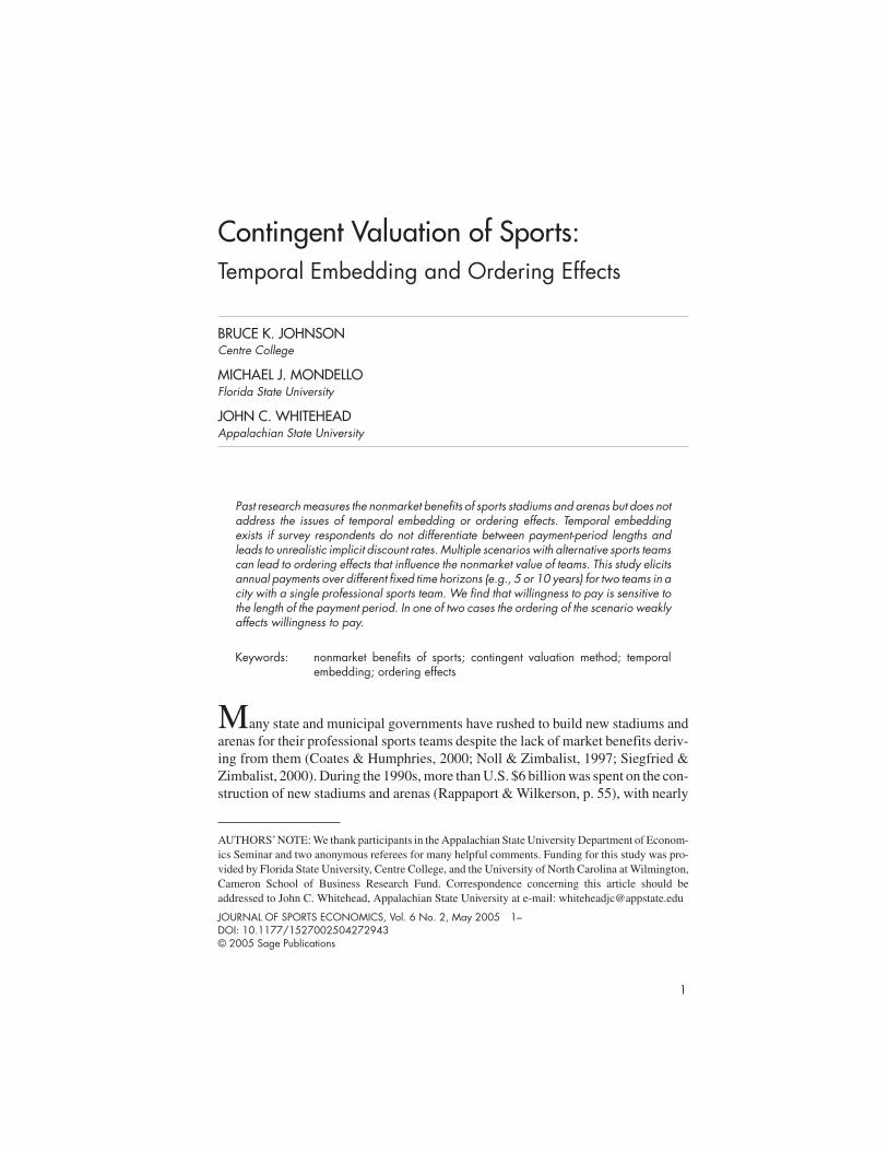
Past research measures the nonmarket benefits of sports stadiums and arenas but does notaddress the issues of temporal embedding or ordering effects. Temporal embeddingexists if survey respondents do not differentiate between payment-period lengths andleads to unrealistic implicit discount rates. Multiple scenarios with alternative sports teamscan lead to ordering effects that influence the nonmarket value of teams. This study elicitsannual payments over different fixed time horizons (e.g., 5 or 10 years) for two teams in acity with a single professional sports team. We find that willingness to pay is sensitive tothe length of the payment period. In one of two cases the ordering of the scenario weaklyaffects willingness to pay.

Keywords: nonmarket benefits of sports; contingent valuation method; temporalembedding; ordering effects

Many state and municipal governments have rushed to build new stadiums andarenas for their professional sports teams despite the lack of market benefits deriv-ing from them (Coates & Humphries, 2000; Noll & Zimbalist, 1997; Siegfried &Zimbalist, 2000). During the 1990s, more than U.S. $6 billion was spent on the con-struction of new stadiums and arenas (Rappaport & Wilkerson, p. 55), with nearly

1

AUTHORS’NOTE: We thank participants in the Appalachian State University Department of Econom-ics Seminar and two anonymous referees for many helpful comments. Funding for this study was pro-vided by Florida State University, Centre College, and the University of North Carolina at Wilmington,Cameron School of Business Research Fund. Correspondence concerning this article should beaddressed to John C. Whitehead, Appalachian State University at e-mail: [email protected]

JOURNAL OF SPORTS ECONOMICS, Vol. 6 No. 2, May 2005 1–DOI: 10.1177/1527002504272943© 2005 Sage Publications

$4 billion of additional construction in progress in 2003 (compiled from figures in“Stadiums and arenas under construction,” 2002, pp. 48-49). A potential explana-tion for the continuing flow of subsidies to sports teams is that teams producenonmarket benefits that are valued highly by the local population (e.g., culturalamenities). When the value of cultural amenities is included in the benefit-costanalysis the total benefits of a new stadium may exceed total costs.

Noll and Zimbalist (1997) suggested that the value of cultural amenities is prob-ably substantial but hard to measure. In an attempt at such measurement, Johnsonand Whitehead (2000) employed a contingent valuation method (CVM) survey toestimate the total benefits that would have been generated by a new basketball arenafor the University of Kentucky and by a minor league baseball stadium forLexington, Kentucky. For both projects, they found that construction costs farexceeded the total benefits and that most of the benefits would have accrued to fansattending games. Johnson, Groothuis, and Whitehead (2001) used a CVM surveyto value the total benefits generated by a major league professional sports team, thePittsburgh Penguins. Although they found large total benefits, their valueamounted to 25% or less of the cost of a new arena. Fenn and Crooker (2003) foundsimilar results for a new Minnesota Vikings stadium.

The existing studies do not address several issues of importance to the valuationof the cultural amenities generated by sports teams. One issue is the temporal natureof the payment streams. As first defined by Kahneman and Knetsch (1992) tempo-ral embedding exists if survey respondents do not consider the length of paymentperiods leading to unrealistic implicit discount rates. Most contingent valuationapplications, including the sports studies mentioned previously, elicit annual pay-ments in perpetuity assuming the annual budget constrains the annual willingnessto pay (WTP). Aggregation over time is then conducted by multiplying annual pay-ments by the time period of the project and applying a market discount rate. Thepresent value of annual WTP is the discounted sum of annual payments.

An alternative is to assume that respondents are constrained by their lifetimewealth and elicit a lump-sum payment or an annual payment over a fixed time hori-zon (e.g., 10 years). In this case, the respondents would apply their individual ratesof time preference to the project and state the present value of WTP. A comparisonof the two question formats in the same survey allows estimation of the implicit dis-count rate used by respondents.

Comparisons of WTP amounts with different payment periods show thatrespondents answer WTP questions with temporal embedding; i.e., with highimplicit discount rates. Kahneman and Knetsch (1992) find that a lump-sum pay-ment and annual payments are not significantly different. Smith (1992) argued thatthe survey design used by Kahneman and Knetsch is flawed leading to the anoma-lous result. Stevens, DeCoteau, and Willis (1997) find that the lump-sum paymentis larger than the annual payments; however, the implicit discount rates are unreal-

2 JOURNAL OF SPORTS ECONOMICS / Month 2005

istically high—annual rates between and 50% and 270% for a public good andweekly rates of 20% to 34% for a private good. The current study employed collegestudents, who have higher rates of time preference than other adults, as respon-dents. Instead of comparing lump-sum and annual payments, Stumborg,Baerenklau, and Bishop (2001) compared WTP with 3-year and 10-year paymentperiods. Perhaps this is one reason they find a more realistic 40% implicit discountrate. Kim and Haab (2003) find implicit discount rates that range from 20% to131%.

These studies have been used to question the validity of the CVM. Comparingthese results to the implicit discount rates obtained from studies of the demand forappliances with varying energy use reviewed by Loewenstein and Thaler (1989),which range from 25% to 243%, suggests that it is not just consumers in contingentmarkets who have high implicit discount rates.

Another issue is the effect of alternative sports teams on WTP values. Johnsonand Whitehead (2000) valued two teams but do not vary the order of the valuationscenarios ignoring the role that the valuation sequence can play. When the sameCVM survey asks for WTP for multiple government policies or public goods insequence, respondents tend to indicate a lower WTP for the second project (Hoehn& Loomis, 1993). Independent valuation, in effect valuing at the beginning of asequence, will lead to the largest of the possible WTP estimates. This result isexpected for the value of public goods estimated with the CVM because of substitu-tion and income effects (Carson, Flores, & Hanemann, 1998; Hoehn & Randall,1989).

Boyle, Welsh, and Bishop (1993) argued that respondent experience plays a rolein the ordering effects of WTP. In an empirical application the order of the valuationscenarios is influential for respondents who are unfamiliar with the survey topic.Those who have experience with whitewater rafting have better formed WTP val-ues and are not influenced by the ordering of the scenario. Stewart, O’Shea,Donaldson, and Shackley (2002) also find evidence that respondent experiencemitigates ordering effects.

The current study considers temporal embedding and ordering effects applied tothe contingent valuation of sports. The case study is professional sports in Jackson-ville, Florida, a city with only one major league sports team. We develop WTP esti-mates for keeping the Jacksonville Jaguars, a National Football League team, inJacksonville and attracting a National Basketball Association team to Jacksonville.In the next section, we describe the CVM survey and the different scenarios.Respondents received different versions of the survey based on the number of yearsthat an annual payment is required and the sequence of the two valuation scenarios.We develop the economic theory and describe tests for temporal embedding andordering effects. Then we describe the data and how the tests are implementedempirically. The results are then described, and conclusions follow.

Johnson et al. / CONTINGENT VALUATION OF SPORTS 3

THE SURVEY

In April 2002 we sent a CVM survey to a random sample, purchased from a pro-fessional sampling firm, of 1,200 households located in Duval County, Florida. Thecity of Jacksonville and Duval County share a merged government. According tothe census of 2000, Duval County contains 72.8% of the population in the Jackson-ville metropolitan statistical area (MSA). The U.S. Postal Service returned 69 ofthe surveys as undeliverable, or 5.75% of the total. Of the 1,131 delivered surveys,421 produced responses, for a response rate of 37.2%. Because some respondentsfailed to complete the surveys, particularly the questions about the demographicvariables, 367 surveys are usable for this analysis.

We employed several strategies to boost the response rate. First, we mailed apostcard to all survey recipients informing them of the survey and asking them towatch for it in their mail in the next few days. The survey cover letter informedrecipients that if they sent back the completed survey postmarked within the nextweek and if they also included their name and address on a separate piece of paper,they would be eligible for a $100 lottery prize. A week after the survey was mailedout, we mailed a reminder postcard to all recipients. The postage-paid survey returnenvelopes were coded so that 1 month after the original mailing we could sendanother copy of the survey to all nonrespondents. We offered another $100 lotteryprize for respondents to the follow-up mailing.

As in many CVM surveys, the typical respondent is older than the typical resi-dent. About 73.7% of the Duval population is age 18 years or older and about 19%is age 55 years or older. The average respondent is age 52 years. As in previoussports CVM surveys, men respond disproportionately more often than women,constituting 69% of the sample. Whites make up 67% of the Duval County popula-tion but 83% of the sample. The census says the average Duval household contains2.51 people. The average sample household size is 2.53. Given the relationshipbetween these demographic variables and income, it is not surprising that theself-reported average household income in the sample, about $58,000, exceededthe estimated Duval household income of $52,949. Of the useable sample, 23respondents did not report income. Income values for these respondents wereimputed with the conditional mean from a multivariate regression model predictingincome.

The survey presented two contingent valuation scenarios designed to elicit WTPfor government policies to (a) ensure that the NFL Jaguars remain in Jacksonvilleand (2) to attract an NBA team to Jacksonville. One half of the surveys presentedthe NFL scenario first and the NBA scenario second. The other one half reversedthe order of the scenarios.

The football scenario was titled, “Should Jacksonville keep the Jaguars frommoving away?” It informed readers that seven times since 1984 NFL teams havemoved to new cities. It then asked readers to suppose that within the next decade the


owner of the Jaguars decides to sell the team to someone who wanted to move themto another city. It then said:

Suppose the city of Jacksonville was able to buy a majority of the team. If the cityowned a majority of the team the Jaguars would never have to leave Jacksonville.Large sums of money from Duval County taxpayers would be needed to buy a major-ity of the team. It has been estimated that it would take annual tax payments of $A forthe next T1 years from each Duval County household to buy a majority of the team.Your total payment would be $A × T1.

The annual tax payments $A and the number of years T1 varied across the surveys,as explained below.1

A dichotomous choice WTP question followed: “Would you be willing to paythe annual tax payments of $A for the next T1 years out of your own household bud-get so that the city of Jacksonville could buy a majority of the Jaguars?” A fol-low-up question asked: “What is the highest annual tax payment you would be will-ing to pay for the next T1 years out of your own household budget to keep theJaguars in Jacksonville?” Response categories are zero, between $0.01 and $4.99,between $5 and $9.99, between $10 and $19.99, between $20 and $39.99, between$40 and $75, and more than $75.

The basketball scenario was titled, “Should Jacksonville try to attract an NBAteam?” After informing readers that NBA teams also move to new cities, it askedthem to suppose that Jacksonville is able to attract an NBA team at some point in thenext decade if Jacksonville upgrades its new arena, currently being built, to NBAstandards. It then said:

Consider the following situation. Large sums of money from Duval County taxpayerswould be needed to upgrade the new arena in Jacksonville to NBA standards. It hasbeen estimated that it would take annual tax payments of $A for the next T2 years fromeach Duval County household to upgrade the new arena. Your total payment would be$A × T2.

The annual tax payments $A and the number of years T2 varied across the sur-veys, as explained below. A dichotomous choice WTP question identical to the firstdichotomous choice question followed.

In the football scenario, the annual tax payment could take the values of $5, $10,$20, or $40 per year, and the number of years could take values of 10 or 20 years. Inthe basketball scenario, the annual tax payment took the same values as those in thefootball scenario. The basketball scenario always presented a payment period onehalf as long as in the football scenario, either 5 or 10 years.

The frequency distributions for NFL and NBA annual WTP by length-of-pay-ment period and ordering are presented in Table 1. More than one half of the WTPamounts are zero. Very few respondents are willing to pay more than $75 each year.Of all respondents, 46% are willing to pay a positive amount (POSITIVE) to keep


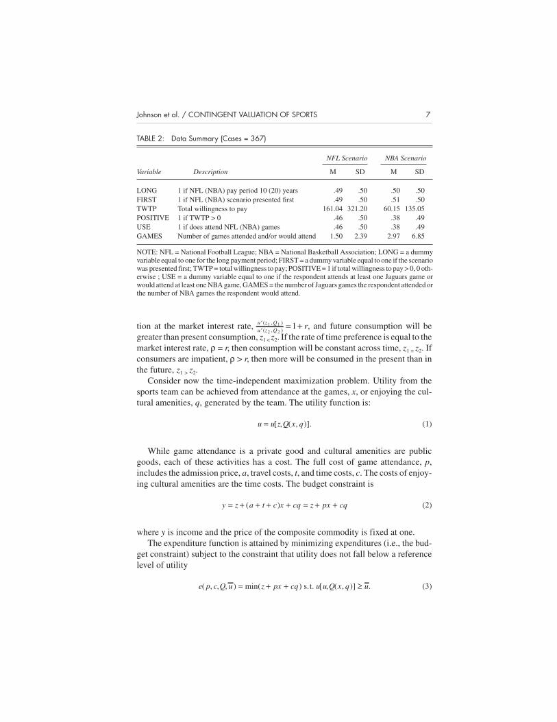
the Jaguars in Jacksonville (Table 2). For those who are willing to pay, the midpointof the annual WTP category is used with the exception of “more than $75” that iscoded as $75. Including the zero WTP responses, the average sum of annual WTPfor the Jaguars across the payment periods (TWTP) is $161. Of all respondents,46% have attended Jaguars games (USE). The average number of games attendedduring the 2001 season (GAMES) was 1.53. Of all respondents, 38% are willing topay a positive amount to attract an NBA team to Jacksonville. The average sum ofannual WTP across the payment periods is $60 for the NBA team. Of all respon-dents, 38% say that they would attend NBA games. The average number of gamesthat they would attend is 2.9.

THEORY

First, to focus on the relationship between the interest rate and the rate of timepreference, consider a two-period utility maximization problem (Silberberg &Suen, 2000). Assume that utility is additively separable over time,U z Q u z Q( , ) ( , )= +1 1 ,u z Q( , )2 2

1+ ρ where U is the intertemporal utility function, u is the utility function in eachtime period, zt is a composite commodity of market goods in time period t, t = 1, 2,Qt is the local sports team and ρ is the rate of time preference. The wealth constraintis that the sum of discounted consumption is equal to the sum of discountedincome,W z yz

ry

r= + = ++ +1 1 1 1

2 2 , where W is wealth and r is the market interest rate.Maximization of utility subject to the wealth constraint leads to the marginal rate

of substitution of present for future consumption, ′′

++=u z Q

u z Qr( , )

( , )1 1

2 2

11 ρ. If consumers are

not impatient, ρ = 0, then future consumption will be traded for present consump-


TABLE 1: Frequency Distribution of Annual Willingness to Pay

NFL NBA

Short Long Short Long

First Second First Second First Second First Second

Zero 56 45 49 49 59 60 68 40Between U.S. $.01and $4.99 11 9 12 8 6 11 7 13

Between $5 and $9.99 13 7 10 14 4 9 9 13Between $10 and$19.99 2 6 3 10 7 2 6 6

Between $20 and$39.99 7 4 1 6 3 7 2 5

Between $40 and $75 10 9 4 4 2 9 2 6More than $75 4 4 7 2 1 5 1 3Total 103 84 86 93 82 103 95 86

NOTE: NFL = National Football League; NBA = National Basketball Association.

tion at the market interest rate, ′′ = +u z Q

u z Qr( , )

( , )1 1

2 21 , and future consumption will be

greater than present consumption, z1 < z2. If the rate of time preference is equal to themarket interest rate, ρ = r, then consumption will be constant across time, z1 = z2. Ifconsumers are impatient, ρ > r, then more will be consumed in the present than inthe future, z1 > z2.

Consider now the time-independent maximization problem. Utility from thesports team can be achieved from attendance at the games, x, or enjoying the cul-tural amenities, q, generated by the team. The utility function is:

u u z Q x q= [ , ( , )]. (1)

While game attendance is a private good and cultural amenities are publicgoods, each of these activities has a cost. The full cost of game attendance, p,includes the admission price, a, travel costs, t, and time costs, c. The costs of enjoy-ing cultural amenities are the time costs. The budget constraint is

y z a t c x cq z px cq= + + + + = + +( ) (2)

where y is income and the price of the composite commodity is fixed at one.The expenditure function is attained by minimizing expenditures (i.e., the bud-

get constraint) subject to the constraint that utility does not fall below a referencelevel of utility

e p c Q u z px cq u u Q x q u( , , , ) min( ) [ , ( , )] .= + + ≥s.t. (3)


TABLE 2: Data Summary (Cases = 367)

NFL Scenario NBA Scenario

Variable Description M SD M SD

LONG 1 if NFL (NBA) pay period 10 (20) years .49 .50 .50 .50FIRST 1 if NFL (NBA) scenario presented first .49 .50 .51 .50TWTP Total willingness to pay 161.04 321.20 60.15 135.05POSITIVE 1 if TWTP > 0 .46 .50 .38 .49USE 1 if does attend NFL (NBA) games .46 .50 .38 .49GAMES Number of games attended and/or would attend 1.50 2.39 2.97 6.85

NOTE: NFL = National Football League; NBA = National Basketball Association; LONG = a dummyvariable equal to one for the long payment period; FIRST = a dummy variable equal to one if the scenariowas presented first; TWTP = total willingness to pay; POSITIVE = 1 if total willingness to pay > 0, 0 oth-erwise ; USE = a dummy variable equal to one if the respondent attends at least one Jaguars game orwould attend at least one NBA game, GAMES = the number of Jaguars games the respondent attended orthe number of NBA games the respondent would attend.

The expenditure function measures the minimum expenditures necessary toachieve the reference utility level and is increasing in the costs of consumption andutility. A necessary condition for consumption of goods related to the local sportsteam is that the team is in the local market; Q = 1 indicates that the team is located inthe local market and Q = 0 indicates that it is located somewhere else.

The indirect utility function is found by maximizing utility subject to the budgetconstraint

v p c Q y u z Q x q y z px cq( , , , ) max [ , ( , )] .= ≥ + +s.t. (4)

The indirect utility function is decreasing in costs and increasing in income. Notethat substitution of the indirect utility function into the expenditure function yieldsincome when terms in the two functions are equivalent. For example, when theexpenditure function is evaluated with the indirect utility function when the sportsteam is in the local market, Q = 1

y e p c Q v p c Q y= = =[ , , , ( , , , )].1 1 (5)

The annual WTP to keep a professional sports team in the local market can bedefined by comparing expenditure functions

AWTP e p c Q v p c Q y e p c Q v p c Qe = = = − = =[ , , , ( , , , )] [ , , , ( , , ,0 1 1 1 y

e p c Q v p c Q y y

)]

[ , , , ( , , , )] .= = = −0 1 1

(6)

where AWTPe is the equivalent surplus and y1 is the income level associated withhaving a team. When the team moves out of the local market, the expenditures nec-essary to achieve the utility level associated with the team is higher than income. Inother words, the annual WTP to keep the sports team in the local market is positive.

The annual WTP to attract a professional sports team in the local market can alsobe defined by comparing expenditure functions

AWTP e p c Q v p c Q y e p c Q v p c Qc = = = − = =[ , , , ( , , , )] [ , , , ( , , ,0 0 1 0 y

y e p c Q v p c Q y

)]

[ , , , ( , , , )].= − = =0 0 1

(7)

where AWTPc is the compensating surplus and y0 is the income level associated withnot having a team. When the team moves into the local market, the expendituresnecessary to achieve the utility level associated with the team are lower thanincome. The annual WTP to attract the sports team in the local market is positive.

The WTP to avoid a decrement when consumers have property rights to the ini-tial resource allocation, Q = 1, is the equivalent surplus measure of welfare


(Bergstrom, 1990). The WTP to gain an increment when consumers have propertyrights to the initial resource allocation, Q = 0, is the compensating surplus measureof welfare. For the same good with equal increments and decrements, it is possibleto make predictions about the relative size of AWTPe and AWTPc. In our case, it isimpossible to compare WTP based on different implicit property rights because wevalue different goods.

TEMPORAL EMBEDDING

Most contingent valuation applications elicit annual payments assuming thecurrent-period budget constrains the WTP. Aggregation over time is then con-ducted by summing annual payments after applying the social discount rate. Thepresent value of annual WTP is

PVAWTP

rtt

t

T

=+=

∑ ( )11

(8)

where ris the social discount rate. Eliciting annual WTP is problematic if therespondents assume they would only pay until the project is completely financed(paying their so-called fair share), say, T = 5, while the analyst aggregates over thelife of the project, say T = 30.

An alternative is to assume that respondents are constrained by their lifetimewealth and elicit a lump-sum payment. In this case, the respondents would applythe individual rate of time preference to the project and state the present value ofWTP as

LSAWTP

tt

T

=+=

∑ ( )11 ρ(9)

where LS is the stated lump-sum WTP, AWTP is the implicit annual WTP of the pol-icy, and ρ is the individual rate of time preference. This approach will tend to under-estimate the present value of WTP if current income constrains respondents and ifthey do not have access to perfect capital markets in which to borrow.

If the average of the individual rates of time preference equals the social dis-count rate, the two approaches will yield the same WTP amount, PV = LS. In theempirical studies reviewed above, estimated rates of time preference are greaterthan market interest rates that serve as measures of the social discount rate. Thisimplies that PV > LS when ρ > r. In other words, the typical approach leads to over-estimates of the present value of aggregate WTP because the rate of discount is toolow.


In this article, in contrast to the typical lump-sum versus annual payments com-parison, respondents face either short or long payment periods. Respondents areasked to state the maximum amount of money that they would be willing to payannually for T years. The total WTP is the undiscounted sum of the annual WTPvalues

TWTP AWTPtt

T

==∑ .

1

(10)

In the case of the Jaguars, respondents face either 10 or 20 years of increased taxes.In the case of the NBA team, respondents face either 5 or 10 years of increasedtaxes. In both cases, the short time period, t = S, is one half that of the long timeperiod, t = L. The rate of time preference can be found by equating the present valueof WTP associated with the annual WTP amounts from the short and long paymentperiods

AWTP AWTPSS

LL

L

T

S

T LS

( ) ( ).

1 111 +=

+==∑∑ ρ ρ

(11)

If respondents ignore the time dimension across surveys and respond withannual WTP amounts that do not differ across short and long time periods,ATWPS = ATWPL, the total WTP with the long time period will be twice as great asthe total WTP with the short time period when 2 × TS = TL

21 1

×⎛

⎝⎜⎜

⎞

⎠⎟⎟ =

= =∑ ∑AWTP AWTPSS

T

LL

TS L

.(12)

For a broad range of realistic WTP amounts when TS is equal to 5 and 10 the rate oftime preference will be greater than 100%. If respondents state annual WTPamounts so that the total WTP for the short and long payment periods are equal (i.e.,AWTPS = 2 × ATWPL) then

AWTP AWTPS LL

T

S

T

===

∑∑ .11

(13)

and the rate of time preference will be zero. For a broad range of realistic WTPamounts when TS is equal to 5 and 10 if respondents adjust their annual WTPamounts so that


21 1

×⎛

⎝⎜⎜

⎞

⎠⎟⎟ >

= =∑ ∑AWTP AWTPSS

T

LL

TS L (14)

the rate of time preference will be greater than zero and less than 100%.

ORDERING EFFECTS

We consider two issues related to ordering effects: substitution and incomeeffects and respondent experience. Consider the independently elicited WTP val-ues for two public goods, Q1 and Q2, and implicitly defined by the indirect utilityfunctions. In this section of the article, the subscripts on Q will refer to differentpublic goods and not different time periods. Annual WTP depends on the quantityof the cross-public good

v Q Q y v Q Q y AWTP( , , ) ( , , )1 2 1 2 10 1= = = − (15)

v Q Q y v Q Q y AWTP( , , ) ( , , ).1 2 1 2 20 1= = = − (16)

WTP is the dollar value subtracted from income that makes the consumer indiffer-ent between keeping the team, Q = 1, and not having the team, Q = 0.

Suppose in the valuation sequence M that WTP for Q1is elicited first and WTPfor Q2 is elicited second:m AWTP AWTP= [ , ]11 22 . If the respondent is willing to payfor the first public good the income available in the second scenario is reduced byAWTP11

v Q Q y v Q Q y AWTP( , , ) ( , , )1 2 1 2 110 0 1 0= = = = = − (17)

v Q Q y v Q Q y AWTP AWTP( , , ) ( , , ).1 2 1 2 11 221 0 1 1= = = = = − − (18)

Consider another valuation sequence N in which WTP for Q2is elicited first andWTP for Q1 is elicited second: N AWTP AWTP= [ , ]21 12 . The WTP values are

v Q Q y v Q Q y AWTP( , , ) ( , , )1 2 1 2 210 0 0 1= = = = = − (19)

v Q Q y v Q Q y AWTP AWTP( , , ) ( , , ).1 2 1 2 21 120 1 1 1= = = = = − − (20)

Implications for the direction of the ordering effects can be determined by compar-ing Equations (17) with (20) and (18) with (19). Because the left-hand side of (17)is less than the left-hand side of (20), the right-hand side of (17) is less than theright-hand side of (20)


v Q Q y AWTP v Q Q y AWTP AWTP( , , ) ( , , )1 2 11 1 2 21 121 0 1 1= = − < = = − − . (21)

By definition, the increase in utility from the increment to Q1 and the decrease inutility from the payment of AWTP21 on the right-hand side of (21) are equal. There-fore, WTP when valued first in the sequence must be greater than WTP when val-ued second in the sequence, ATWP11 > ATWP12, for the inequality to hold. Whenvalued second in the sequence, WTP is lower because of an increasingly bindingincome constraint, y – ATWP12 < y. WTP is also negatively affected by the availabil-ity of a substitute good, Q1 = 1.

A similar argument can be made for the effects of ordering on WTP for Q2. Inthis case, the WTP when valued first in a sequence will be greater than the value forthe same public good elicited second in the sequence, ATWP 21 > ATWP22, becauseof income and substitution effects. The implication of these comparisons is thatWTP values are not unique; they depend on the policy context in which the publicgoods are delivered.

Consider next the role of respondent experience and a public good for which allrespondents have experience, such as the consumption and other activities relatedto the Jacksonville Jaguars. When respondents formulate WTP values for the Jag-uars they are familiar with the characteristics of the good that they are paying for. Incontrast, respondents do not have experience with a NBA team and are not familiarwith the characteristics of the public goods associated with a NBA team. When for-mulating WTP values, the lack of experience may create uncertainty about WTPand the order of the scenarios may affect the WTP estimates.

Whitehead, Blomquist, Hoban, and Clifford (1995) argue that prior knowledgeof the resource, gained from experience, is a necessary condition for positive WTP.Survey information can lead to positive WTP; however, the WTP statements fromuninformed respondents will be relatively less valid and reliable than those frominformed respondents. In the context of ordering effects, this suggests that unin-formed respondents will be more likely to be influenced by survey and other factorsaffecting WTP, such as the order of the scenario, starting point dollar amounts, andother survey information.

Yea saying may be a factor for uninformed respondents. Some survey respon-dents prefer to please the interviewer rather than answer survey questions honestly.Yea-saying behavior in CVM surveys leads to respondents stating that they wouldbe willing to pay for the public good in an attempt to please the interviewer even iftheir utility would fall after payment. Yea-saying respondents will be less likely torespond that they would be willing to pay for a public good that is presented secondin a sequence if they have already responded with a positive WTP to the first good inthe sequence. Respondents with experience with the public good (i.e., Jaguar fans)might be less prone to yea-saying behavior.


EMPIRICAL MODEL

We focus our empirical modeling efforts on the continuous WTP data con-structed from the follow-up interval WTP questions. With continuous WTP ques-tions, respondents first decide whether to pay anything and then, conditional onpositive WTP, the magnitude of WTP. Total annual WTP is positive if utility withthe team is greater than utility without the team

TWTPAWTP T v p c Q y v p c Q y

AWTP T=

× > = ≥ =× =

0 1 0

0

if

if

( , , , ) ( , , , )

v p c Q y v p c Q y( , , , ) ( , , , ).

= < =⎧⎨⎩ 1 0

(22)

The second decision, the magnitude of total WTP, is equal to annual WTP, asdefined above, multiplied by the length of the payment period. The expected valueof total WTP is the product of the probability that total WTP will be positive andexpected total WTP given that WTP is positive

E TWTP TWTP E TWTP TWTP( ) ( ) ( | ).= > × >π 0 0 (23)

There are several approaches to analyzing these data. Two of the more obviousare the Tobit and the Cragg models (Bockstael, Strand, McConnell, & Arsanjani,1990). The Cragg model allows the determinants of positive WTP and the magni-tude of WTP to differ. The single-equation Tobit model constrains the determinantsof both decisions to be equal. In the current study, more than one half of the respon-dents report zero WTP values, suggesting substantially different processes fordeciding whether to pay and, if so, how much. In the empirical results below, likeli-hood ratio tests indicate that the Cragg model is superior to the Tobit for these data.

The Cragg model offers an alternative to the Tobit that decomposes WTPdirectly. The Cragg model first employs a probit model to estimate the probabilityof positive total WTP

π βσ

( )TWTPX> = ′⎛

⎝⎜

⎞⎠⎟0 1

1 1

1

Φ(24)

where Φ is the standard normal distribution function, X is a vector of independentvariables, β is a vector of coefficients, and σ is the standard deviation of the regres-sion. The subscript refers to the first decision on whether to pay. The truncatedregression model employs only the positive WTP data to estimate expected totalWTP

E TWTP TWTP X( | )

( )

( )

> = ′ +

=−

0

1

2 2 2

2

2

β σ λ

λ φ θθΦ

(25)


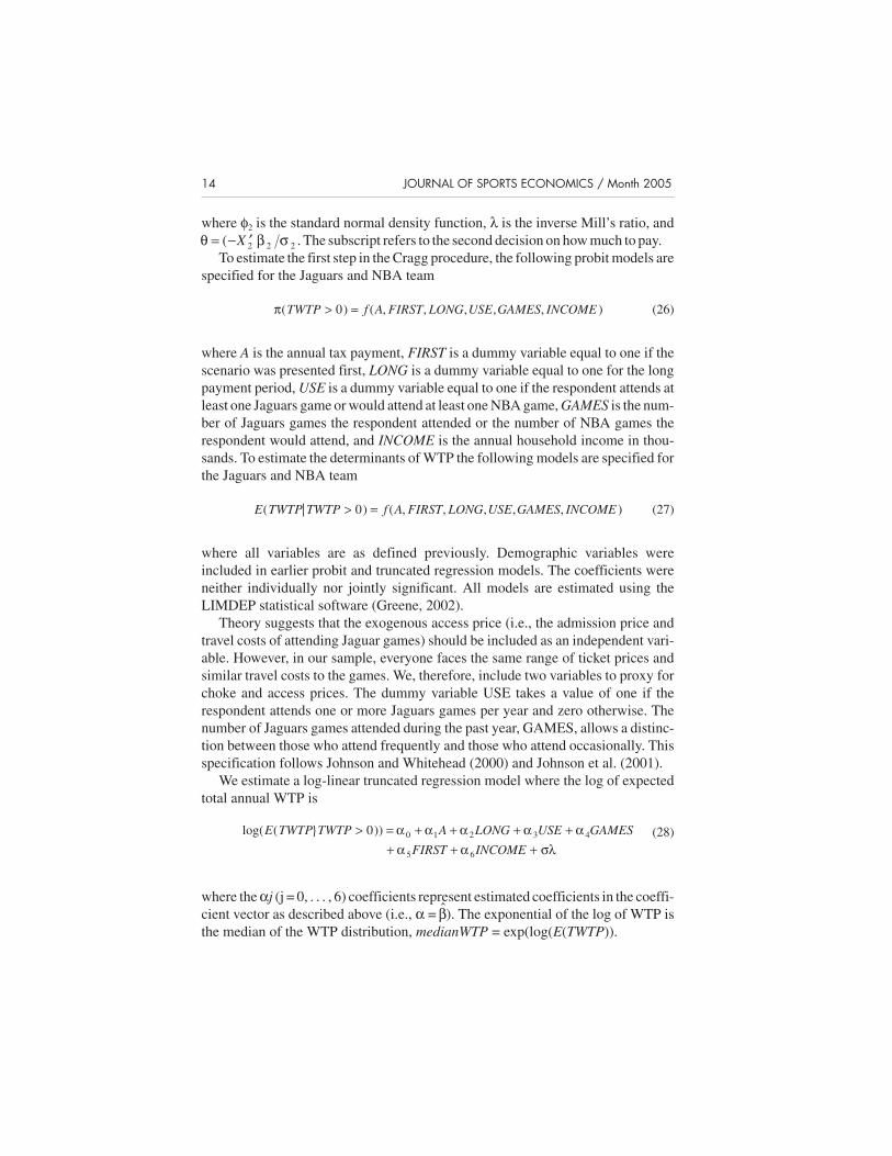
where φ2 is the standard normal density function, λ is the inverse Mill’s ratio, andθ β σ= − ′( X 2 2 2 . The subscript refers to the second decision on how much to pay.

To estimate the first step in the Cragg procedure, the following probit models arespecified for the Jaguars and NBA team

π( ) ( , , , , , )TWTP f A FIRST LONG USE GAMES INCOME> =0 (26)

where A is the annual tax payment, FIRST is a dummy variable equal to one if thescenario was presented first, LONG is a dummy variable equal to one for the longpayment period, USE is a dummy variable equal to one if the respondent attends atleast one Jaguars game or would attend at least one NBA game, GAMES is the num-ber of Jaguars games the respondent attended or the number of NBA games therespondent would attend, and INCOME is the annual household income in thou-sands. To estimate the determinants of WTP the following models are specified forthe Jaguars and NBA team

E TWTP TWTP f A FIRST LONG USE GAMES INCOME( | ) ( , , , , , )> =0 (27)

where all variables are as defined previously. Demographic variables wereincluded in earlier probit and truncated regression models. The coefficients wereneither individually nor jointly significant. All models are estimated using theLIMDEP statistical software (Greene, 2002).

Theory suggests that the exogenous access price (i.e., the admission price andtravel costs of attending Jaguar games) should be included as an independent vari-able. However, in our sample, everyone faces the same range of ticket prices andsimilar travel costs to the games. We, therefore, include two variables to proxy forchoke and access prices. The dummy variable USE takes a value of one if therespondent attends one or more Jaguars games per year and zero otherwise. Thenumber of Jaguars games attended during the past year, GAMES, allows a distinc-tion between those who attend frequently and those who attend occasionally. Thisspecification follows Johnson and Whitehead (2000) and Johnson et al. (2001).

We estimate a log-linear truncated regression model where the log of expectedtotal annual WTP is

log( ( } ))E TWTP TWTP A LONG USE GAMES> = + + + ++

0 0 1 2 3 4

5

α α α α αα FIRST INCOME+ +α σλ6

(28)

where the αj (j = 0, . . . , 6) coefficients represent estimated coefficients in the coeffi-cient vector as described above (i.e., α = �β). The exponential of the log of WTP isthe median of the WTP distribution, medianWTP = exp(log(E(TWTP)).


The effect of the tax amount on total WTP is a test of starting point bias from theinitial dichotomous choice WTP question. Starting point bias exists when a sug-gested value serves as an anchor for subsequent valuation responses. Becauseordering effects are more likely to occur when consumers lack experience withgoods, starting point bias is more likely to affect the NBA scenario than the Jaguarsscenario. When measuring the log of expected total WTP, starting point bias can bepurged by setting the tax amount equal to zero

log( ) ( ) .TWTP A Xj jj

= + = + +=∑α α α σλ0 1

2

6

0(29)

TESTING FOR TEMPORAL EMBEDDING AND ORDERING EFFECTS

The long scenario, measured by the LONG dummy variable, may affect WTP.Given a positive WPT, it may affect the magnitude of WTP. However, there are noobvious theoretical reasons why the long scenario should affect the probability of apositive amount. Even if respondent total WTP is $1 spread over 20 years, the cor-rect survey response is the interval “between $.01 and $4.99.” Therefore, we do notexpect a statistically significant effect unless respondents wish to avoid longerpayment commitments.

The magnitude of the LONG dummy variable on expected total WTP is a mea-sure of the log sum of the annual WTP amounts during the second one half of thelong payment period. The coefficient on the LONG dummy variable will be posi-tive if total WTP is higher with the longer payment period. In other words, α2 willbe zero if respondents have a zero rate of time preference and positive if the rate oftime preference is greater than zero.

Alternatively, setting LONG equal to zero and one when measuring expectedWTP measures the log of total WTP for the short and long payment periods

log( ) ( ) ( )TWTP A LONG XS j jj

= + = + = + +=∑α α α α σλ0 1 2

3

6

0 0(30)

log( ) ( ) ( ) .TWTP A LONG XL j jj

= + = + = + +=∑α α α α σλ0 1 2

3

6

0 1(31)

The hypothesis test for temporal embedding is

H TWTP TWTP

HA TWTP TWTPS L

S L

0 2

2

:

: .

× ≤× >

(32)


If twice the total WTP amounts in the short payment period is greater than the totalWTP in the long payment period then the implicit rate of time preference will bebetween 0% and 100%. This indicates that respondents are cognizant of the tempo-ral dimensions of the scenario, and temporal embedding does not arise. Note, how-ever, that unrealistically high implicit discount rates could still be a problem eventhough temporal embedding, as defined here, does not arise.

By contrast, the tests for ordering effects are straightforward. If the placement ofthe CVM scenario affects the probability of a positive WTP amount then the probitcoefficient on the FIRST variable will be statistically different from zero. Withordering effects, we expect a positive coefficient. In other words, the size of theWTP market is expected to be larger when the CVM scenario is placed first in asequence. In the truncated regression model, a positive and statistically significantcoefficient estimate on the FIRST variable, α5 > 0, indicates that total annual WTPis greater when the NFL team or NBA team and/or arena is valued first in thesequence. A statistically insignificant coefficient indicates that WTP is not affectedby the order of the CVM scenario.

RESULTS

The estimation results from the probit models conducted as the first step in theCragg model appear in Table 3. The NBA and NFL models use the same vector ofindependent variables to estimate the probability that a respondent reports a posi-tive WTP value for the basketball and football teams. This allows for a direct com-parison between the factors that affect positive WTP in the two scenarios.


TABLE 3: Probit Regression Models: Dependent Variable = Positive (Cases = 367)

NBA NFL

b t Ratio b t Ratio

Constant –1.295 –5.36 –.564 –2.73TAX (A) –.009 –1.68 .001 .20FIRST .616 3.94 .044 .32LONG .303 1.94 –.013 –.09USE .991 4.75 .727 3.82GAMES .082 2.93 .050 1.24INCOME .001 .42 .0001 .03Model χ2 138.08 50.29

NOTE: NBA = National Basketball Association; NFL = National Football League; TAX (A) = annualtax payment; FIRST = a dummy variable equal to one if the scenario was presented first; LONG = adummy variable equal to one for the long payment period; USE = a dummy variable equal to one if therespondent attends at least one Jaguars game or would attend at least one NBA game; GAMES = thenumber of Jaguars games the respondent attended or the number of NBA games the respondent wouldattend; INCOME = the annual household income in thousands.

In the basketball scenario, the magnitude of the tax amount from the dis-crete-choice WTP question has a negative effect on the probability of a positiveWTP. This indicates a form of starting point bias in which high stated costs lead toavoidance of paying anything. The bias does not appear in the NFL model. The longpayment period leads to a greater probability of a positive WTP in the NBA sce-nario but not in the football scenario. This is a surprising result and may indicatethat the 5-year payment period was unrealistically short leading to zero WTPresponses that indicate a protest of the unrealistic contingent market.

Those respondents who would attend at least one game are more likely to pay apositive amount for basketball, as would those who reported attending at least onefootball game would be more likely to pay in the football scenarios. The probabilityof a positive amount in the NBA scenario increases with the number of games thatthe respondent expects to attend; however, the number of games does not affect theprobability of being willing to pay for the NFL. If the basketball scenario was pre-sented first, the probability of a positive WTP for the NBA is greater. However, noordering effect appears in the NFL model. Given the differences in the resultsacross basketball and football scenarios, respondents distinguish between the twoscenarios and regard football and basketball differently.

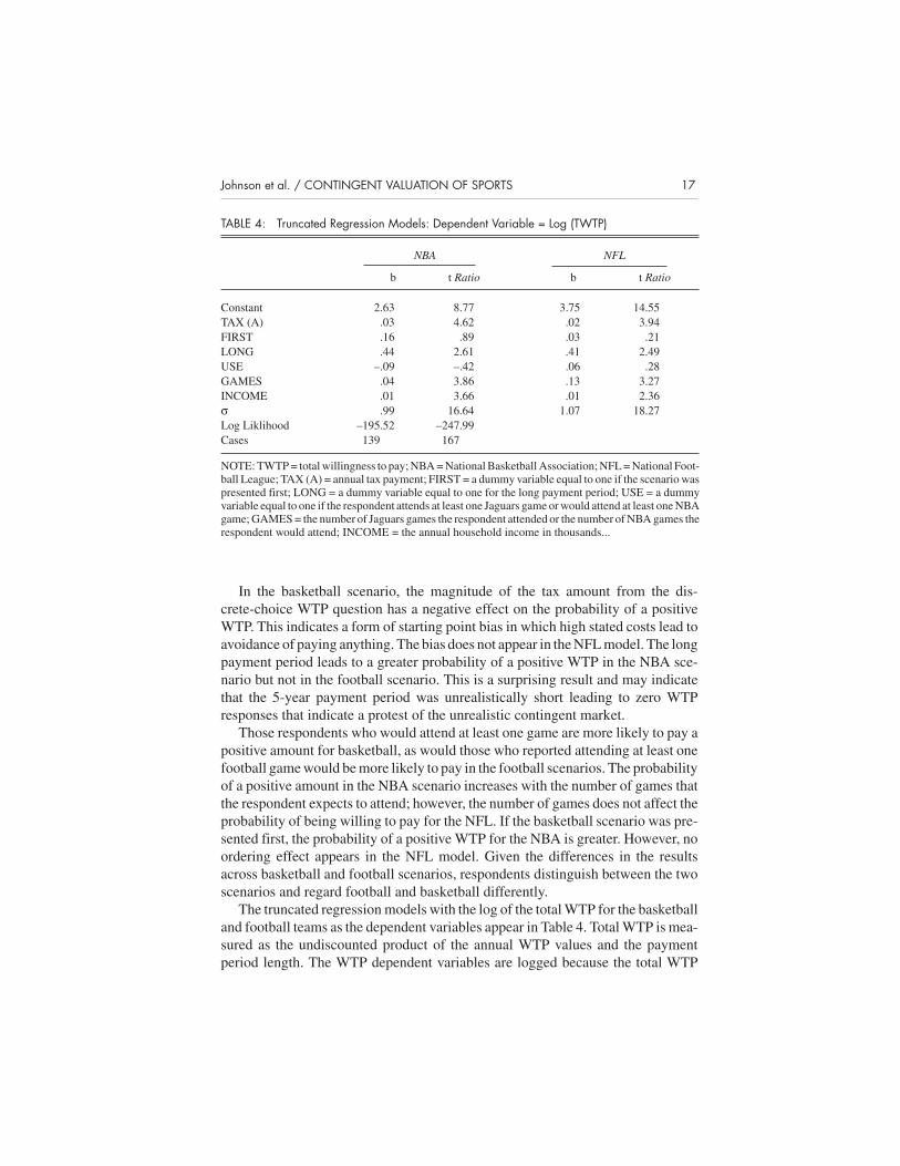
The truncated regression models with the log of the total WTP for the basketballand football teams as the dependent variables appear in Table 4. Total WTP is mea-sured as the undiscounted product of the annual WTP values and the paymentperiod length. The WTP dependent variables are logged because the total WTP


TABLE 4: Truncated Regression Models: Dependent Variable = Log (TWTP)

NBA NFL

b t Ratio b t Ratio

Constant 2.63 8.77 3.75 14.55TAX (A) .03 4.62 .02 3.94FIRST .16 .89 .03 .21LONG .44 2.61 .41 2.49USE –.09 –.42 .06 .28GAMES .04 3.86 .13 3.27INCOME .01 3.66 .01 2.36σ .99 16.64 1.07 18.27Log Liklihood –195.52 –247.99Cases 139 167

NOTE: TWTP = total willingness to pay; NBA = National Basketball Association; NFL = National Foot-ball League; TAX (A) = annual tax payment; FIRST = a dummy variable equal to one if the scenario waspresented first; LONG = a dummy variable equal to one for the long payment period; USE = a dummyvariable equal to one if the respondent attends at least one Jaguars game or would attend at least one NBAgame; GAMES = the number of Jaguars games the respondent attended or the number of NBA games therespondent would attend; INCOME = the annual household income in thousands...

variables are nonnormally distributed, and the truncated regression model assumesa normal distribution. Because of the log-linear functional form the coefficient esti-mates are interpreted as the percentage change in total annual WTP.

In the NBA model, the coefficient on the annual tax amount variable is statisti-cally significant. The coefficient on this variable indicates that for each one-dollarincrease in the annual tax amount, total WTP increases by 3%. This is evidence thatrespondents anchored their WTP amounts to the tax amount. If the basketball sce-nario is presented first, WTP is no higher. WTP in the long scenario is 44% greaterthan in the short scenario. The dummy variable for whether the respondent wouldattend at least one game has no effect on WTP; however, WTP does increase withthe number of games. The coefficient indicates that an additional game increasestotal annual WTP by 4%, above and beyond the expected ticket price and othercosts of game access. Income is a statistically significant variable. As incomeincreases by $1,000, WTP increases by 1% indicating that the basketball team is anormal good.

Estimation of the NFL WTP model yields results qualitatively similar to those ofthe NBA model in that the same variables tend to be statistically significant. As inthe NBA model, starting point bias exists, with each one-dollar increase in theannual tax amount increasing total WTP by 2%. The order of the scenario does notsignificantly affect the total WTP amount. Total WTP is 41% higher in the long sce-nario. The dummy variable for whether the respondent attended at least one foot-ball game has no effect on total WTP. However, as in the case of the NBA, the num-ber of games the respondent attends increases total WTP. An additional gameincreases total WTP by 13%. Note that the effect of games on total WTP increaseswith game scarcity (i.e., 8 home games compared to 41). Although the coefficienton income is positive, it is not statistically significant.

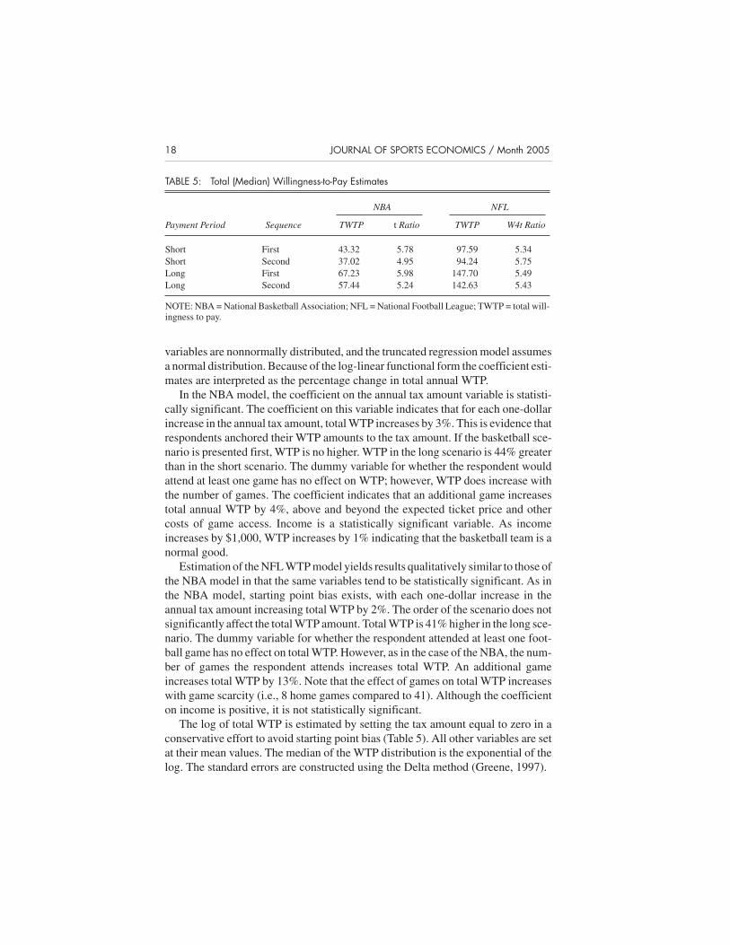
The log of total WTP is estimated by setting the tax amount equal to zero in aconservative effort to avoid starting point bias (Table 5). All other variables are setat their mean values. The median of the WTP distribution is the exponential of thelog. The standard errors are constructed using the Delta method (Greene, 1997).


TABLE 5: Total (Median) Willingness-to-Pay Estimates

NBA NFL

Payment Period Sequence TWTP t Ratio TWTP W4t Ratio

Short First 43.32 5.78 97.59 5.34Short Second 37.02 4.95 94.24 5.75Long First 67.23 5.98 147.70 5.49Long Second 57.44 5.24 142.63 5.43

NOTE: NBA = National Basketball Association; NFL = National Football League; TWTP = total will-ingness to pay.

The (median) total WTP for the basketball team and/or arena during the shortpayment period (5 years) is $43. The implied annual WTP is $8.66. During the longpayment period (10 years), total WTP is $67, and the annual WTP is $6.72. Thetotal WTP during the short payment period is $24 greater than that of the additionalWTP during the second half of the long payment period. This difference is statisti-cally different from zero (t = 2.43). In other words, twice the total WTP in the shortpayment period is greater than total annual WTP in the long payment period. Thisindicates no temporal embedding. The implicit rate of time preference that equatesthe present value of the WTP amounts, assuming that the first payment occurs in thefirst year of the payment period (not the current year), for these two paymentschedules is 28%.

In the second NBA scenario, total WTP is $37 in the short payment period and$57 in the long payment period. The annual WTP amounts are $7.40 and $5.74,respectively. The difference of $20 in total WTP between payment periods is statis-tically different from zero (t = 2.40). Again, the total WTP amount in the long pay-ment period is less than twice the total WTP in the short payment period. Theimplicit rate of time preference is 28%.

In the first scenario, total WTP for the football team is $98 over the short pay-ment period (10 years) and $148 over the long payment period (20 years). Theannual WTP amounts are $9.76 and $7.39, respectively. The total WTP amount inthe long payment period is less than twice the total annual WTP in the short pay-ment period. The $50 difference in total annual WTP during the payment periods isstatistically different from zero (t = 2.30). Again, we find no evidence of temporalembedding. The implicit rate of time preference is 12% in the first footballscenario.

Total WTP in the second scenario is $94 and $143 with the short and long pay-ment periods, respectively. The annual WTP amounts are $9.42 and $7.13, respec-tively. Again, the total WTP amount in the long payment period is less than twicethe total WTP in the short payment period. The $48 difference in WTP is statisti-cally different from zero (t = 2.23). The implicit rate of time preference is 12% inthe second football scenarios.

For the NBA team, there is a $6 and $10 decrease in the total WTP amounts fromthe first to second scenarios in the short and long payment periods, respectively.The ordering effects are an increase of $3 and $5 in total WTP from the first and sec-ond scenarios for the football team. However, none of these differences are statisti-cally different from zero at the p = .10 level.

CONCLUSIONS

In this article, we estimate the WTP for two professional sports teams and con-sider temporal embedding and ordering effects. Temporal embedding is an issuewhen the length of the payment period is not made explicit and survey respondentsand researchers use different lengths of payment periods. In this case, aggregated


benefit estimates will be biased. Ordering effects are an issue when multiple WTPscenarios are presented to respondents. Typically, WTP for the same good is lowerwhen placed second in a sequence of scenarios relative to when it is placed first. Wefind no evidence of temporal embedding and ordering effects. Furthermore, theWTP estimates are internally valid. Respondents are more likely to be willing topay if they attend games. The magnitude of WTP is greater for those who attendgames and for those with higher incomes (in one of two scenarios).

In our tests for temporal embedding, the total annual WTP amounts in the longpayment period are less than twice the total annual WTP in the short paymentperiod. This indicates that respondents applied a positive discount rate to their WTPstatements, agreeing to pay higher annual WTP amounts if the number of yearsrequired to pay is lower. The implicit discount rates for the NFL scenario, 12%, arevery reasonable. The implicit discount rates for the NBA scenario are more thantwice as high, 28%, but still lower than estimates of the implicit discount rate fromthe CVM literature. These discount rates are in the range of market interest ratesoffered by credit card companies and finance companies to households with highdefault risk and lower than most of the implicit discount rates obtained fromrevealed behavior reviewed by Loewenstein and Thaler (1989).

The difference in discount rates between the NBA and NFL scenarios is of someconcern. It should be expected that respondents will have similar rates of time pref-erence across commodities. The difference in discount rates may be because of thedifferent length of time periods for the two scenarios. This result is similar to thatobtained by Kim and Haab (2003) who find that shorter payment schedules lead tohigher implicit discount rates. The result may also be due to the valuation of differ-ent commodities and the lack of respondent experience with the NBA. Stevens et al.(1997) find that implicit discount rates differ for different commodities with thediscount rate for a private good exceeding the discount rate for a public good.

This and other CVM studies to date that estimate implicit discount rates havefound that the rates are greater than market interest rates that are typically used todiscount annual WTP values when aggregating over time. For example, many stud-ies contrast the present value of discounted benefits from the 2% and 7% rates rec-ommended by the U.S. General Accounting Office and the U.S. Office of Manage-ment and Budget. Use of either of these discount rates will lead to overestimates ofaggregate benefits when CVM respondents state annual WTP values with higherrates of time preference greater than market interest rates.

In our tests for ordering effects, we find no ordering effects in the NFL models.Past research has argued that experience with the good might lead to a lack of order-ing effects. This is consistent with our NFL results because Jacksonville residentshave a number of years of experience with the Jaguars. The probability of positiveWTP is greater when the NBA team and/or arena appears first in the valuationsequence. This type of ordering effect, which affects the market size of WTP, maybe due to a lack of experience with an NBA team and will lead to an increase in


WTP when aggregated to the population. The bias in total WTP from ordered CVMscenarios is not statistically significant.

These results suggest that the typical CVM that elicits annual WTP amountsshould explicitly state the length of the payment period to avoid aggregating WTPestimates over a time period longer than respondents perceive. This may be espe-cially true with the contingent valuation of sports teams, stadiums, and arenas thathave large up-front costs. However, if stadiums and arenas are financed by munici-pal bonds the payment period could be 30 years or longer. Even so, the length of thepayment period should always be made explicit when it could be interpreted invarious ways by respondents.

Another concern is that this, and other, CVM studies focused on temporal issuesassume that expected inflation is zero. As is well known in the macroeconomics lit-erature, positive expected inflation will lead to growing expected nominal incomeover time. As with fixed rate mortgages and automobile loan payments, the abilityto pay fixed nominal amounts increases over time. Therefore, positive expectedinflation will lead to larger nominal WTP for normal goods over time. In our case,the effect of expected inflation will narrow the difference in the nominal annualWTP amounts for the short and long payment periods. Discounting for expectedinflation will cause real total WTP amounts in short and long payment periods toconverge and lead to smaller implicit discount rates than those reported here. Asexpected inflation increases, the implicit discount rate decreases. Future studies oftemporal embedding should consider the issue of expected inflation, expectedfuture income, and their effects on WTP.

Other than an ordering effect for the size of the WTP market, ordering of CVMscenarios does not appear to be a major problem with this sports economics appli-cation. However, this result could be an artifact of some characteristic of the currentstudy. Best practice is not to ignore the potential for ordering effects. Future studieswith multiple scenarios should vary the appearance of each scenario in thesequence of scenarios.

NOTES

1. As pointed out by a referee, saying that “large sums of money . . . would be needed” may negativelybias WTP. Bohara et al. (1998) found that information about the total cost of a project has no effect onWTP elicited with a dichotomous choice question but negative effects on WTP elicited with anopen-ended question. We recognize that the cost information may lead to a negative bias in WTP.

REFERENCES

Bergstrom, J. C. (1990). Concepts and measures of the economic value of environmental quality: Areview. Journal of Environmental Management, 31, 215-228.


Bockstael, N. E., Strand, I. E., McConnell, K. E., & Arsanjani, F. (1990). Sample selection bias in theestimation of recreation demand functions: An application to sportfishing. Land Economics, 66(1),40-49.

Bohara, A., McKee, M., Berrens, R., Jenkins-Smith, H., Silva, C., & Brookshire, D. (1998). Effect ofcost and group-size information on willingness to pay responses: Open-ended vs. dichotomouschoice. Journal of Environmental Economics and Management, 35, 142-163.

Boyle, K. J., Welsh, M. P., & Bishop, R. C. (1993). The role of question order and respondent experiencein contingent-valuation studies. Journal of Environmental Economics and Management, 25(1),S80-S99.

Carson, R., Flores, N. E., & Hanemann, W. M. (1998). Sequencing and valuing public goods. Journal ofEnvironmental Economics and Management, 36(3), 314-323.

Coates, D., & Humphreys, B. (1999). The growth effects of sport franchises, stadia, and arenas. Journalof Policy Analysis and Management, 18(4), 601-624.

Fenn, A. J., & Crooker, J. R. (2003, July). The willingness to pay for a new Vikings stadium. Paper pre-sented at the 2003 Western Economics Association Meetings, Denver, CO.

Greene, W. H. (1997). Econometric analysis (3rd ed.). Englewood Cliffs, NJ: Prentice Hall.Greene, W. H. (2002). LIMDEP version 8.0: User’s manual. Bellport, NY: Econometric Software.Hoehn, J. P., & Loomis, J. B. (1993). Substitution effects in the valuation of multiple environmental pro-

grams. Journal of Environmental Economics and Management, 25(Pt. 1), 56-75.Hoehn, J. P., & Randall, A. (1989). Too many proposals pass the benefit cost test. American Economic

Review, 79, 544-551.Johnson, B. K., Groothuis, P. A., & Whitehead, J. C. (2001). The value of public goods generated by a

major league sports team: The CVM approach. Journal of Sports Economics, 2(1), 6-21.Johnson, B. K., & Whitehead, J. C. (2000). Value of public goods from sports stadiums and arenas: The

CVM approach. Contemporary Economic Policy, 18(1), 48-58.Kahneman, D., & Knetsch, J. L. (1992). Valuing public goods: The purchase of moral satisfaction. Jour-

nal of Environmental Economics and Management, 22(1), 57-70.Kim, S.-I., & Haab, T. C. (2003). Temporal sensitivity of willingness to pay and implied discount rates

(Working Paper). Columbus: The Ohio State University, Department of Agricultural, Environmen-tal, and Development Economics.

Loewenstein, G., & Thaler, R. H. (1989). Intertemporal choice. Journal of Economic Perspectives, 3(4),181-194.

Noll, R. G., & Zimbalist, A. (Eds.). (1997). Sports, jobs, and taxes: The economic impact of sports teamsand stadiums. Washington, DC: Brookings Institution.

Rappaport, J., & Wilkerson, C. (2001, January). What are the benefits of hosting a major league sportsfranchise? Federal Reserve Bank of Kansas City Economic Review, 55-86.

Siegfried, J., & Zimbalist, A. (2000). The economics of sports facilities and their communities. Journalof Economic Perspectives, 14(3), 95-114.

Silberberg, E., & Suen, W. (2000). The structure of economics (3rd ed.). New York: McGraw-Hill.Smith, V. K. (1992. Arbitrary values, good causes, and premature verdicts: Comment. Journal of Envi-

ronmental Economics and Management, 22, 71-89.Stadiums and arenas under construction. (2002, December 30). Sports Business News, pp. 48-49.Stevens, T. H., DeCoteau, N. E., & Willis, C. E. (1997). Sensitivity of contingent valuation to alternative

payment schedules. Land Economics, 73(1), 140-148.Stewart, J. M., O’Shea, E., Donaldson, C., & Shackley, P. (2002). Do ordering effects matter in willing-

ness-to-pay studies of health care? Journal of Health Economics, 21, 585-599.Stumborg, B. E., Baerenklau, K. A., & Bishop, R. C. (2001). Nonpoint source pollution and present val-

ues: A contingent valuation study of Lake Mendota. Review of Agricultural Economics, 23(1),120-132.


Whitehead, J. C., Blomquist, G. C., Hoban, T. L., & Clifford, W. B. (1995). Assessing the validity andreliability of contingent values: A comparison of on-site users, off-site users and non-users. Journalof Environmental Economics and Management, 29(2), 238-251.

John C. Whitehead obtained his Ph.D. in economics from the University of Kentucky. He is anassociate professor in the Department of Economics at Appalachian State University. Hisresearch interests include various applications of stated preference methods including the con-tingent valuation of sports.

Michael Mondello obtained his Ph.D. from the University of Florida in higher education with afinance concentration. He currently teaches sport finance in the Graduate Sport ManagementProgram at The Florida State University. His research interest focus on financial and/or eco-nomical issues related to sports including revenue sharing, contingent valuation, ticket pricing,and the professional development of the academic field of sport management.

Bruce K. Johnson earned his Ph.D. in economics from the University of Virginia and is the JamesGraham Brown Professor of Economics at Centre College in Danville, KY. His research andwriting interests include economic policy and the economics of sports.


Documents

Contingent Valuation of Sports - Appalachian State Universitywhiteheadjc/research/papers/jse272943.pdf · 10.1177/1527002504272943 JOURNAL OF SPORJohnson et al. / CONTINGENT VALUATION