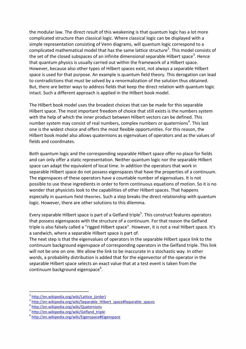
Continuity Equation for Quaternionic Quantum Fields

By Ir J.A.J. van Leunen

Retired physicist & software researcher

Location: Asten, the Netherlands

Website: http://www.crypts-of-physics.eu/

Communicate your comments to info at that site.

Last version: November 19, 2011

Abstract The continuity equation is specified in quaternionic format. It means that the density and current of the considered “charge” is combined in a quaternionic probability amplitude distribution (QPAD). Next, the Dirac equation is also put in quaternionic format. It is shown that it is a special form of continuity equation. Further it is shown that two other quaternionic continuity equations can be derived from the quaternionic Dirac equation. The square and the squared modulus of the QPAD play an essential role in these new equations. Further, a whole series of equivalent equations of motions is derived from the possible sign flavor couplings. The corresponding particles are identified as member of the standard model. The coupling constant of the particles can be computed from their fields. In this way all known particles in the standard model can be identified. Keywords: quaternionic partial differential equation, continuity equation, balance equation, Dirac equation, Majorana equation, quaternionic field theory, quaternionic field sign flavors, standard model.

Preface This is an update of the paper that was published under the title “Quaternionic continuity equation for charges”. Some of the findings in this paper are certainly not unique and also not the first of its kind. The paper of Finkelstein ea, which is referred at the bottom, showed that similar things were already discovered in the sixties of the last century. Welch discovered similar things for quarks.

Essentials of the Hilbert book model The subject of this paper is a part of the Hilbert book model. For that reason a short introduction of that model is presented here. The Hilbert book model is a simple model of physics that is strictly based on the axioms of quantum logic1. Quantum logic is very similar to classical logic, but one of the axioms of quantum logic is weaker than the corresponding axiom of classical logic. This axiom concerns

1 http://en.wikipedia.org/wiki/Quantum_logic

the modular law. The direct result of this weakening is that quantum logic has a lot more complicated structure than classical logic. Where classical logic can be displayed with a simple representation consisting of Venn diagrams, will quantum logic correspond to a complicated mathematical model that has the same lattice structure2. This model consists of the set of the closed subspaces of an infinite dimensional separable Hilbert space3. Hence that quantum physics is usually carried out within the framework of a Hilbert space. However, because also other types of Hilbert spaces exist, not always a separable Hilbert space is used for that purpose. An example is quantum field theory. This derogation can lead to contradictions that must be solved by a renormalization of the solution thus obtained. But, there are better ways to address fields that keep the direct relation with quantum logic intact. Such a different approach is applied in the Hilbert book model. The Hilbert book model uses the broadest choices that can be made for this separable Hilbert space. The most important freedom of choice that still exists is the numbers system with the help of which the inner product between Hilbert vectors can be defined. This number system may consist of real numbers, complex numbers or quaternions4. This last one is the widest choice and offers the most flexible opportunities. For this reason, the Hilbert book model also allows quaternions as eigenvalues of operators and as the values of fields and coordinates. Both quantum logic and the corresponding separable Hilbert space offer no place for fields and can only offer a static representation. Neither quantum logic nor the separable Hilbert space can adapt the equivalent of local time. In addition the operators that work in separable Hilbert space do not possess eigenspaces that have the properties of a continuum. The eigenspaces of these operators have a countable number of eigenvalues. It is not possible to use these ingredients in order to form continuous equations of motion. So it is no wonder that physicists look to the capabilities of other Hilbert spaces. That happens

especially in quantum field theories. Such a step breaks the direct relationship with quantum logic. However, there are other solutions to this dilemma. Every separable Hilbert space is part of a Gelfand triple5. This construct features operators that possess eigenspaces with the structure of a continuum. For that reason the Gelfand triple is also falsely called a "rigged Hilbert space". However, it is not a real Hilbert space. It's a sandwich, where a separable Hilbert space is part of. The next step is that the eigenvalues of operators in the separable Hilbert space link to the continuum background eigenspace of corresponding operators in the Gelfand triple. This link will not be one on one. We allow the link to be inaccurate in a stochastic way. In other words, a probability distribution is added that for the eigenvector of the operator in the separable Hilbert space selects an exact value that at a test event is taken from the continuum background eigenspace6.

2 http://en.wikipedia.org/wiki/Lattice_(order)

3 http://en.wikipedia.org/wiki/Separable_Hilbert_space#Separable_spaces

4 http://en.wikipedia.org/wiki/Quaternions

5 http://en.wikipedia.org/wiki/Gelfand_triple

6 http://en.wikipedia.org/wiki/Eigenspace#Eigenspace

Instead of directly applying a probability density distribution we use a quaternionic probability amplitude distribution7. However, the square of the modulus of this distribution is a probability density distribution. It determines the probability of presence. We can separate the amplitude distribution into a charge density distribution and a current density distribution. For a while the interpretation of these charges and currents will be left in the middle. In the described way we achieve several goals at one blow. It opens the possibility to apply continuity equations8. Continuity equations are also called balance equations. The equations of motion of the charge-bearing quanta are in fact continuity equations. By using this approach, we have created the possibility to analyze the movement of these quanta, whatever those quanta may be. This interpretation also determines the kind of operator that is involved. It is an operator that delivers an observable, which changes dynamically in the realm of a background continuum space. We now have a powerful weapon in the hands to describe the behavior of quanta. Unfortunately, neither the separable Hilbert space that is extended with quaternionic probability amplitude distributions, nor the similarly extended quantum logic can represent anything else than a static status quo. Since the charge distributions and flow distributions are known in the form of probability distributions at least something is known about how the following static status quo will look. Despite the containment of these these preconditions the somewhat extended model is still a static model and not a dynamic model. The solution is obvious. It consists of an ordered sequence of consecutive static models. Each static model consists of a sandwich in the form of a Gelfand triple and the stochastic but static links that exist between the separable Hilbert space and the Gelfand triple. The picture that emerges is that of a book where the consecutive pages represent successive sandwiches. The page number acts as a progress counter. It is a global working counter. It adds a parameter that represents the Hilbert space wide progress for each Hilbert space in the Hilbert book model. So this parameter is not our common notion of time, but the progression counter has certainly much relation with it. This model shows that no direct relationship exists between the progression parameter and the position of a quantum. The progression is represented by a Hilbert space wide parameter. The position is an eigenvalue of a corresponding operator. Only when the quantum moves, a relationship emerges between these quantities. A uniform movement can be described by a Galileo transformation or, when a maximum speed exists, by a Lorentz transformation9. The Lorentz transformation introduces the notions of proper time and coordinate time. It offers the opportunity to bind coordinate time and space into the notion of spacetime. We now have a dynamic model that can display the movement of quanta and can describe the behavior of related fields.

7 http://en.wikipedia.org/wiki/Probability_amplitude

8 http://en.wikipedia.org/wiki/Continuity_equation

9 http://en.wikipedia.org/wiki/Lorentz_transformation#Derivation

The beauty of this model is that it is literally based on pure logic. Only mathematics is used in order to extend that foundation. The main extra ingredient is the stochastic link between eigenvalues in the separable Hilbert space and eigenspaces in the Gelfand triple.

Quaternion sign flavors Quaternion fields come in four sign flavors10: . The sign flavors are determined by sign selections. Three sign selections play a role. One of them corresponds to conjugation.

And with the same symbolic:

But we will not apply that symbol very often. The background coordinate system has its own kind of sign flavor. The sign flavor of the background coordinate system can act as a reference for comparing quaternion field sign flavors. A quaternionic field will stick with one and no more than one sign flavor. We will use the

symbol for the quaternionic field that has the same sign flavor as the local background coordinate system. The background coordinate system can be curved. In that case we use the local tangent space that acts as a quaternionic number space. In the investigated continuity equations, pairs of field sign flavors will be treated that belong to the same base field .

We sometimes call the flipped field and stands for the flip. The continuity equation will use one of the pair as the analyzed field and the other pair member as the source field. Each choice of the pair of field sign flavors will result in a different equation. The same equation may accept different basic fields ( ). The standard model appears to use three different field configurations for . Each of these configurations has its own set of coupling factors. This paper does not explain why these three field configurations exist. Each ordered pair represents an elementary particle type category. Each such pair corresponds to a specific continuity equation of motion, which is also an equation of motion. Some categories appear in triplets. The members of the triplet are coupled to directions of imaginary base vectors. Apart for the categories for which the coupling factor equals zero, each category corresponds with three different coupling factors

Sign flavor Flip Imaginary Handedness Isotropy

10

The notion of “sign flavor” is used because for elementary particles “flavor” already has a different meaning.

(1)

(2)

(3)

base vectors conjugation: 3 switch isotropic

double flip: 2 neutral anisotropic

single flip: 1 switch anisotropic

No flip 0 neutral isotropic

flip 3 switch anisotropic

The quaternionic nabla operator uses the sign flavor of the background coordinate system.

Continuity equation When is interpreted as a charge density distribution, then the conservation of the corresponding charge is given by the continuity equation:

Total change within V = flow into V + production inside V

∫

∮

∫

∫

∫⟨ ⟩

∫

Here is the normal vector pointing outward the surrounding surface S, is the velocity at which the charge density enters volume V and is the source density inside V. In the above formula stands for

It is the flux (flow per unit area and unit time) of . The combination of and is a quaternionic skew field and can be seen as a probability amplitude distribution (QPAD).

can be seen as an overall probability density distribution (PDD). is a charge density distribution. is the current density distribution. Depending on their sign selection, quaternions come in four sign flavors. In a QPAD the quaternion sign flavors do not mix. So, there are four QPAD sign flavors. Still these sign flavors can combine in pairs or in quadruples. The quaternionic field contains information on the distribution of the considered charge density as well as on the current density , which represents the transport of this charge density.

(1)

(2)

(3)

(4)

(5)

Where can be seen as a probability density of finding the center of charge at position , the probability density distribution can be seen as the probability density of finding the center of the corresponding wave package at location . is the Fourier transform of . The dimension of is , the dimension of is ]. The factor c has dimension . is an arbitrary dimension. It attaches to the charge. The conversion from formula (2) to formula (3) uses the Gauss theorem11. This results in the law of charge conservation

⟨ ( )⟩

⟨ ⟩

⟨ ⟩ ⟨ ⟩

⟨ ⟩

The blue colored ± indicates quaternionic sign selection through conjugation of the field . The field is an arbitrary differentiable vector function.

⟨ ⟩ is always divergence free. In the following we will neglect . In Fourier space the continuity equation becomes:

⟨ ⟩ This equation represents a balance equation for charge (or mass) density. Here is the charge distribution, is the current density. This only treats the real part of the full equation. The full equation runs:

⟨ ⟩ ( )

⟨ ⟩ ⟨ ⟩

( )

⟨ ⟩ ⟨ ⟩

11

http://en.wikipedia.org/wiki/Divergence_theorem

(6)

(7)

(8)

(9)

(10)

( ( ))

The red sign selection indicates a change of handedness by changing the sign of one of the imaginary base vectors. (Conjugation also causes a switch of handedness). If temporarily no creation and no annihilation occur, then these equations reduce to equations of motion.

⟨ ⟩ ( )

⟨ ⟩

⟨ ⟩

The field can be split in a (relative) stationary background and the moving private field .

If is a constant then

⟨ ⟩

( )

⟨ ⟩ ( )

The continuity equation has a direct relation to a corresponding conservation law12. The conserved quantity is or its integral

∫

Noether’s theorem13 provides the relation between conserved quantities, differentiable symmetries and the Lagrangian14.

The Dirac equation The QPAD can be used to define a charge probability density and probability current density. See http://www.vttoth.com/qt.htm.

The Dirac equation appears to be a special form of continuity equation.

12

http://en.wikipedia.org/wiki/Conservation_law 13

http://en.wikipedia.org/wiki/Noether's_theorem 14

http://en.wikipedia.org/wiki/Lagrangian#Lagrangians_in_quantum_field_theory

(11)

(12)

(13)

(14)

(15)

(16)

(17)

(18)

(1) (2)

The Dirac equation runs

and represent the matrices that implement the quaternion behavior including the sign selections of quaternions for complex fields. We keep the sign selections of the background coordinate system fixed. Thus and only influence the elements of spinor .

[

]

[

]

[

]

[ ]

There exist also a relation between and the Pauli15 matrices :

[ ] [

] [

]

This combination is usually represented in the form of gamma matrices16. These matrices are not used in this paper. They are used when a complex Hilbert space must handle quaternionic behavior. Transferring the matrix form of the Dirac equation into quaternionic format delivers two quaternionic fields and that couple two equations of motion.

The mass term couples and . The fact decouples and .

Thus the fields are each other’s quaternionic conjugate. Reformulating the quaternionic equations gives

15

http://en.wikipedia.org/wiki/Pauli_matrices 16

http://en.wikipedia.org/wiki/Gamma_matrices

(2)

(3)

(4)

(5)

(6)

(7)

(8)

(9)

(10)

(11)

For the conjugated field holds

This implements the reverse flip. The corresponding particle is the antiparticle.

( ) ( )

Summing the equations gives via

⟨ ⟩ the result

⟨ ⟩ The difference gives

Just reversing the sign flavors does not work. The corresponding equation contains extra terms:

⟨ ⟩ ⟨ ⟩

⟨ ⟩ Thus if the reverse equation fits, then it will concern another field configuration that will not fit the original equation.

⟨ ⟩

Compare with the continuity equations

⟨ ⟩

And

(12)

(13)

(14)

(15)

(16)

(17)

(18)

(19)

(20)

(21)

(22)

This means that

Thus in the Dirac equation the mass term is a source term that depends on the (conjugate) field. The following definitions specify another continuity equation:

⟨ ⟩

⟨ ⟩

| |

The field is real and non-negative and represents a probability density distribution. This result defines two new continuity equations. has a Minkowski signature.

The interpretation of as the probability density distribution of presence leads to:

∫

∫

The coupling factor for the antiparticle is the same. The field has an intrinsic spin17:

∫ ∫ ∫

The sign flavor flip reverses the spin.

Interactions The interaction free equation can be extended with interactions with other fields.

17

http://www.plasma.uu.se/CED/Book/EMFT_Book.pdf Section: Conservation of angular momentum, formula 4.70a

(23)

(24)

(25)

(26)

(27)

(28)

(29)

(30)

(31)

(32)

(33)

The field is right covariant with . The field is left covariant with . The two can be

combined in Q-covariance. is a coupling constant. Thus here is the two sided covariant derivative18. The field represents a source. For the interaction field holds

⟨ ⟩

is the d’Alembert operator The wave equation for the electromagnetic field in vacuum is

Besides of the one sided covariance also a Q covariance is possible due to the application of a quaternion waltz19.

Prospect The original Dirac equation can be transformed into two quaternionic equations:

The reverse equations are more complicated:

⟨ ⟩

⟨ ⟩ We will analyze whether this is more general principle. For example the Majorana equation is to a certain extend similar to the Dirac equation.

The Majorana equation The Majorana equation20 differs from the Dirac equation in the way that the sign selection of the field is changed.

18

See paragraphs on covariant and Q-covariant derivative 19

Fermion and boson equations; Q covariant derivative 20

http://en.wikipedia.org/wiki/Majorana_equation

(1)

(2)

(3)

(4)

In the Majorana equation the mass term contains the sign flavor of the field . In this case only two imaginary base vectors change their sign. This sign selection does not switch handedness. Three independent directions are possible. (That fact may not be observable).

For the conjugated equation holds:

The sign selection only switches a single imaginary base vector. Like the conjugation, it switches the handedness of Thus the conjugated equation does not switch the handedness. Again three independent directions are possible. Neutrinos are supposed to obey the Majorana equation. When the Majorana equation holds, then

|

|

∫( )

∫( )

∫| |

∫

∫

∫| |

∫| |

For the conjugated field holds:

|

|

∫( )

∫

Another version of equations for neutral particles is:

For the conjugated equation holds:

And for the coupling factor:

(1)

(2)

(3)

(4)

(5)

(6)

(7)

(8)

(9)

(10)

∫( )

∫

This selection obviously concerns a boson21.

The third category sign flavor switch Apart from the Dirac equation and the Majorana equation, a third category equation is possible. In this equation the mass term flips the sign of only one imaginary base vector. As a result the handedness flips as well. The sign flavor of the background coordinate system can act as a reference for comparing quaternion sign flavors. The quaternionic nabla operator uses that same sign flavor. With respect to the background sign flavor, three different possibilities for the choice of the flipped imaginary base vector exist. It will become clear that this category corresponds to quarks. The corresponding equation is:

The index runs over three color versions r, g and b. For the conjugated equation holds:

For each color an up version

and a down version

exists. The up version

obeys equation (1). The down version obeys equation (2). The down version is the conjugated version of the up version. When this third category equation holds, then

|

|

∫

∫

∫ | |

∫( )

|

|

21

Fermion and boson equations

(1)

(2)

(3)

(4)

(5)

(6)

(7)

Intermezzo:

⟨ ⟩

(

)

Another version of the third category is

For the conjugated equation holds:

∫( )

∫( )

In contrast to the ( ) flip, the ( ) flip and the (

) flip are strongly

anisotropic. The three choices for the flipped imaginary base vector may be linked with color charges. The antiparticles have anti-color. The particles and antiparticles may be linked with the color charges and the up and down versions of quarks. The fact that only one of the three, or with the second version two of the three imaginary base vectors are flipped may account for the respective electrical charges, which are .or .

The cross-sign flavor equations

These equations describe the situation that a flip is made from a

field to a

field or

vice versa. The direction seems to play no role.

(8)

(9)

(10)

(11)

In fact equation 2 is the conjugated equation of equation 1. The sign flavor switch affects three imaginary base vectors and flips the handedness. As a consequence the particles have a full electric charge. It concerns two particles, the and the bosons. These bosons carry electrical charges.

∫ ( )

∫ ( )

∫ (

)

∫ ( )

The non-sign flavor flip category In this category no switch is performed. The field couples with itself. The corresponding equation is:

For the antiparticle holds:

And for the mass holds

∫( )

∫ ( )

∫( )

The equation describes neutral particles. For the probability density no integral source or leakage exists. Thus must be zero.

Fermion and boson equations Elementary particles are identified by a pair of quaternionic field sign flavors. The antiparticle corresponds to the conjugated pair. The type of sign flavor switch determines the charge of the particle. From this combination it is not clear what the spin of the particle

(1)

(2)

(3)

(4)

(5)

(6)

(1)

(2)

(3)

will be. It certainly has something to do with the handedness of the transported field (The field that is subjected to Elementary particles with zero mass are not coupled and appear to be bosons. With the W

bosons the transported field is in condition or . For all fermions the transported field

is in condition or .

The Z boson is a stranger. The Z boson might correspond to equation (4a) rather than to equation (4b). Eight fermion equations exist. Their interaction free forms are:

The general form of the equation is:

For the antiparticle:

(1)

(2)

(3)

(4)

(5)

(6)

(7)

(8)

(9)

(10)

(11)

Elementary fermions are elementary particles that are based on a coupled pair of

field sign flavors of which the transported member has sign flavor 𝜓 or 𝜓 . Elementary bosons are elementary particles that are based on non-coupled field sign flavors or on a coupled pair of field sign flavors of which the transported

member has sign flavor 𝜓 or 𝜓

For all particles holds:

⟨ ⟩

∫

Further, the equation for coupling factor

∫

∫

∫| |

An equivalent of the Lagrangian may look like

Survey of couplings In the following table the attribution of particle names is speculative.

RLrl e Diff Coupling Particle Multiplet

RL -1 3 fermion electron 1

LR 1 3 fermion positron 1

Rl -⅓ 1 fermion down-quark 3 colors

lR ⅓ 1 boson ? 3 colors

Lr ⅔ 1 fermion up-quark 3 colors

rL -⅔ 1 boson ? 3 colors

Rr 0 2 fermion neutrino 3?

rR 0 2 boson ? 3?

Ll 0 2 fermion ? 3?

lL 0 2 boson Z 3?

rl -1 1 boson 3?

lr 1 1 boson 3?

RR 0 0 0 boson photon

LL 0 0 0 boson photon

rr 0 0 0 boson gluon 3?

ll 0 0 0 boson gluon 3?

Colophon: RLrl; switch by 3, 2 or 1 imaginary base vectors e; electric charge of particle Diff; number of imaginary base vectors difference

(12)

(13)

(14)

(15)

(16)

(17)

Coupling; the field sign flavors that are coupled Fermion/boson; Particle; elementary particle category Multiplet; multiplet structure The neutrinos, Z and W bosons might show multiplicity. In the standard model three versions of fermion mass factors exist. These versions are not (yet) explained by this model. Remarkably, in the table several places for particles are still open. (lR, rL, rR, Ll)

Coupling factors The integral probability densities are:

∫( )

∫| |

∫( )

∫( )

∫| |

∫| |

The coupling factors are:

Primary Coupling factor reverse Coupling factor

∫

∫

∫( )

∫( )

∫(

)

∫(

)

∫ (

)

∫ (

)

Most particle categories of the SM appear with three different coupling factors. This corresponds with three different field configurations of . This paper does not explain that extra diversity.

Interactions In complex quantum field theory, interactions are derived from covariant derivatives. In quaternion field theory this is not that straight forward. The problem is caused by the fact that for quaternionic fields in general:

On the other hand quaternionic fields are interesting because a field can rotate inside another field under the influence of a quaternion waltz:

The result is Q-covariance.

Covariant derivative The covariant derivative plays a role in the Lagrangian and in the equation of motion. The covariant derivative of field is defined as

This is interesting with respect to a gauge transformation of the form

The field has a modulus that is equal to one:

We suppose that a field exists such that

A new version of the derivative can be obtained by a corresponding vector potential transformation

The following inequality holds in general for quaternionic functions.

( ) ( )

However, we assume that it is an equality for .

(1)

(2)

(1)

(2)

(3)

(4)

(5)

(6)

(7)

(8)

( )

Thus, with that transformation pair not only the modulus of the function stays invariant but also the modulus of the covariant derivative stays invariant. Further

Above the right sided covariant derivative is defined

The left sided covariant derivative is defined as:

We will use for both left sided and right sided covariant derivative:

Multiplication with a unitary factor corresponds with a displacement in the canonical conjugate space, thus with a shift of the momentum of the field.

Q Covariant derivative The Q covariant derivative22 relates to quaternionic field transformations of the form

This is the quaternion waltz. Let the imaginary field be defined by:

( )

22 Principle of General Q Covariance; D. Finkelstein, J. M. Jauch, S. Schiminovich and D. Speiser; Journal of

Mathematical Physics volume 4, number 6, June 1963, 788-796

(9)

(10)

(11)

(12)

(13)

(1)

(2)

(3)

(4)

The following step is questionable, because with quaternionic functions in general

However we consider the rule valid for this special case. In fact we apply the covariant case twice.

( ) ( )

The general equation of motion is:

Applying the quaternion waltz gives:

[

]

Where

Thus, the general equation of motion due to the waltz is

This equation describes the equation of motion including interactions that are due to the effect of the quaternion waltz under the influence of another field ( ). The interpretation of the Q-covariant derivative is that the particle to which and belong not only moves due to the nabla operator, but also rotates with respect to an outside field , which takes the particle in a quaternion waltz23.

English quaternion waltz When the rotation is slow compared to the current , then it becomes interesting to analyze an infinitesimal rotation. The quaternionic value of is close to 1. Thus

is imaginary. Let us investigate the transform .

23

For an explanation of the quaternion waltz, see the Hilbert book model: http://www.crypts-of-physics.eu/OntheoriginofdynamicsBoek2.pdf, part two

(5)

(6)

(7)

(8)

(9)

(10)

(11)

(12)

(13)

(14)

Forbidden region Fermions have asymmetric permutation wave functions. This fact has only significance when two or more states are considered. Let us consider the situation that the two states are completely identical24 and are nearly at the same location. In that case the superposition of the two states is given by:

| | | | | The plus sign holds for bosons and the minus sign holds for fermions. The images of the two cases are:

Boson pair Fermion pair

Symmetric distribution Asymmetric distribution

This is a two dimensional model, but it explains the general idea. Below the cut through the center of the asymmetric distribution is shown. When this is compared with the same cut of the squared modulus, then it reveals a forbidden region for the asymmetric distribution.

The particles were put at the closest possible position. Before the displacement occurs, the direction of the displacement is undefined. Thus the forbidden region has a spherical shape. When fermions go to their next position, they must step over the forbidden region. Bosons do not have that restriction.

Interpreting the flip event The equations of motion indicate that a flip of field sign flavor occurs. The charge density distribution specifies the probability where this flip occurs. The current density distribution represents the transport of the location where the flip may occur.

24

http://en.wikipedia.org/wiki/Identical_particles

The flip event can be observed. This is then the event of observing the corresponding quantum. The observation represents the interaction with another particle. The flip event may represent an electric charge and it may represent a color charge. Photons and gluons are flipping at every progression step. That is why their coupling constant delivers zero.

Interpreting coupling factors The gravitation field, which is a tensor field rather than a quaternionic field, is an administrator of the local curvature rather than that it is the cause of local curvature. The value of the local metric tensor accurately registers all aspects of the local curvature. From the gravitation field it is possible to derive centers of gravitation on which the field can be thought to be anchored. Such a center need not be the location of an actual cause. It can be the center of the activity of a local geometric anomaly, such as a black hole. Such a center is a (virtual) position that can be at a location where space does not even exist. This is possible when two coordinate systems are considered. One flat and the other curved. The curved system features geometric anomalies. In this way it becomes possible to consider a black hole as a geometric anomaly, such that within which nothing, not even space exists. Instead space at its border is curved such that no information can penetrate that border. Every particle, elementary or not, that approaches the border is ripped apart and part of the debris is attached to the border of the BH. The rest of the debris escapes from the process. It can be imagined that elementary particles that possess mass will also have a geometric anomaly at their center. The curvature at the border of that anomaly forms a center of gravity. The fact that the particle is formed by anti-symmetric private fields will already explain the presence of such a local hole. Private fields of elementary particles are formed by pairs of coupled sign flavors of the same quaternionic probability amplitude distribution. The coupling factor that characterizes the coupling of the two sign flavors might also determine the curvature of the local geometric anomaly.

Interpreting the equations of free movement The equations of movement are best interpreted when an extra differentiation step is added:

It means that a coupled oscillation takes place when the quantum moves. In case of leptons this means that:

The coupled oscillation takes place along the direction in which the electron moves. The anisotropic coupled quanta oscillate free in one or two directions and oscillate coupled along the direction of movement.

References The contents of this paper is taken from part two of the Hilbert book model: http://www.crypts-of-physics.eu/OntheoriginofdynamicsBoek2.pdf This paper uses a simpler form of Q-covariance than the paper: Principle of General Q Covariance; D. Finkelstein, J. M. Jauch, S. Schiminovich and D. Speiser; Journal of Mathematical Physics volume 4, number 6, June 1963, 788-796 For other investigations of similar quaternionic equations of movement, see: Colored Quaternion Dirac Particles of Charges 2/3 and -1/3; http://arxiv.org/abs/0809.0484 Quaternion Dirac Equation and Supersymmetry; http://arxiv.org/abs/hep-th/0701131