MIT OpenCourseWare http://ocw.mit.edu Continuum Electromechanics For any use or distribution of this textbook, please cite as follows: Melcher, James R. Continuum Electromechanics. Cambridge, MA: MIT Press, 1981. Copyright Massachusetts Institute of Technology. ISBN: 9780262131650. Also available online from MIT OpenCourseWare at http://ocw.mit.edu (accessed MM DD, YYYY) under Creative Commons license Attribution-NonCommercial-Share Alike. For more information about citing these materials or our Terms of Use, visit: http://ocw.mit.edu/terms.

8

Statics and Dynamics of SystemsHaving a Static Equilibrium

li-

~·.

8.1 Introduction

In general, it is not possible for a fluid to be at rest while subject to an electric or magneticforce density. Yet, when a field is used to levitate, shape or confine a fluid, it is a static equi-librium that is often desired. The next section begins by identifying the electromechanical conditionsrequired if a state of static equilibrium is to be achieved. Then, the following three sectionsexemplify typical ways in which these conditions are met. From the mathematical viewpoint, the subjectbecomes more demanding if the material deformations have a significant effect on the field. Thesesections begin with certain cases where the fields are not influenced by the fluid, and end with modelsthat require numerical solution.

The magnetization and polarization static equilibria of Sec. 8.3 also offer the opportunity toexplore the attributes of the various force densities from Chap. 3, to exemplify how entirely differentdistributions of force density can result in the same incompressible fluid response and to emphasizethe necessity for using a consistent force density and stress tensor.

Given a static equilibrium, is it stable? This is one of the questions addressed by the remainingsections, which concern themselves with the dynamics that result if an equilibrium is disturbed. Sometypes of electromechanical coupling take place in regions having uniform properties. These are exem-plified in Secs. 8.6-8.8. However, most involve inhomogeneities. The piecewise homogeneous modelsdeveloped in Secs. 8.9-8.16 are chosen to exemplify the range of electromechanical models that can bepictured in this way.

The last sections, on smoothly inhomogeneous systems, serve as an introduction to a viewpointthat could equally well be exemplified by a range of electromechanical models. Once it is realizedthat the smoothly inhomogeneous systems can be regarded as a limit of the piecewise inhomogeneous sys-tems, it becomes clear that all of the models developed in this chapter have counterparts in this domain.

The five electromechanical models that are a recurring theme throughout this chapter are sum-marized in Table 8.1.1.

Table 8.1.1. Electromechanical models.

Model Approximation

Magnetization (MQS) or polarization (EQS) No free current or charge

Instantaneous magnetization or polarization

Flux conserving (MQS) T << T

Charge conserving (EQS) T << T or Tmig

Instantaneous magnetic diffusion (MQS) T >> TmInstantaneous charge relaxation (EQS) T >> Te or Tmig

Magnetization and polarization models for incompressible motions require an inhomogeneity in mag-netic or electric properties. The remaining interactions involve free currents or charges which gener-ally bring in some form of magnetic diffusion or charge relaxation (or migration). How such rateprocesses come into the electromechanics is explicitly illustrated in the sections on homogeneous sys-tems, Secs. 8.6 and 8.7. However, in the more complex inhomogeneous systems, the last four models ofTable 8.1.1 not only result in analytical simplifications, but give insights that would be difficultto glean from a more general but complicated description. "Constant potential" continua fall in thecategory of instantaneous charge relaxation models.

STATIC EQUILIBRIA

8.2 Conditions for Static Equilibria

Often overlooked as an essential part of fluid mechanics is the subject of fluid statics. A re-minder of the significance of the subject is the equilibrium between the gravitational force densityand the hydrostatic fluid pressure involved in the design of a large dam. On the scale of the earth'ssurface, where g is essentially constant, the gravitational force acting on a homogeneous fluidobviously is of a type that can result in a static equilibrium.

Except for scale, electric and magnetic forces might well have been the basis for Moses' partingof the Red Sea. Fields offer alternatives to gravity in the orientation, levitation, shaping or

Secs. 8.1 & 8.2

~l

(0)

(b)

«[9I

(c)

(d)

Fig. 8.2.1. (a) Electric field used to shape a "lens" of conducting liquid resting on a pool ofliquid metal. Molten plastics and glass are sufficiently conducting that they can be re­garded as "perfect" conductors. (b) Polarization forces used to orient a highly insulatingliquid in the top of a tank regardless of gravity. The scheme might be used for providingan artificial bottom in cryogenic fuel storage tanks under the zero-gravity conditions ofspace. (c) Liquid metal levitator that makes used of forces induced by a time-varying mag­netic field. At high frequencies, the flux is excluded from the metal, and hence the fieldstend toward a condition of zero shearing surface force density. (d) Cross-sectional viewof axisymmetric magnetic circuit and magnetizable shaft with magnetizable fluid used to sealpenetration of rotating shaft through vacuum containment.

1-3otherwise controlling of static fluid configurations. Examples are shown in Fig. 8.2.1.

For what force distributions can each element of a fluid be in static equilibrium? If the ex­ternal electric or magnetic force density is Fe, then the force equation reduces to

++-V'(p - pg·r) (1)

This expression is a limiting form of Eq. 7.4.4 with the velocity zero. Even if effects of viscosity

1.

2.

3.

J. R. Melcher, D. S. Guttman and M. Hurwitz, "Die1ectrophoretic Orientation," J. Spacecraft andRockets i, 25 (1969).

E. C. Okress et al., "Electromagnetic Levitation of Solid and Molten Metals," J. Appl. Phys. Q,545 (1952).

R. E. Rosensweig, G. Misko1czy and F. D. Ezekiel, "Magnetic-Fluid Seals," Machine Design March 281968. ' ,

Sec. 8.2 8.2

are included in the model, because v = 0, Eq. 1 still represents the static equilibrium. Thus, it isalso the static limit oZ Eq. 7.4.4. The curl of a gradient is zero. So, the curl of Eq. 1 gives anecessary condition on Fe for static equilibrium:

V x Fe = 0 (2)

To achieve a static equilibrium, the force density must be the gradient of a scalar, -VS. Then Eq. 1becomes

V(p - pg'r + S) = 0 (3)

which will be recognized as Eq. 7.8.4 in the limit v = 0.

More often than not, in an electromagnetic field a fluid does not reach a static equilibrium.Electromagnetic forces do not generally satisfy Eq. 2. Fields designed to achieve an irrotational forcedensity are exemplified by Secs. 8.3-8.5.

These sections also illustrate that stress balance at interfaces is similarly restricted. A cleanstatic interface is incapable of sustaining a net electrical shearing surface force density. Formally,this is seen from the interfacial stress balance, Eq. 7.7.6, which states that the normally directedpressure jump and surface tension surface force density must be balanced by the electrical force density.The last, f Te[ 0 nj, is in general not normal to the interface.

To be specific about what types of interfaces do satisfy this requirement, consider an interfacehaving a normal vector in the x direction. Then, nj = 6jx and for the directions i 0 x the surfaceforce density is

OTix - E=DxD = EinDx (EQS)(4)

Tix f = HIBx B= Bx (MQS)

In writing the second equalities, advantage is taken of the continuity of tangential E (EQS) and normal

' (MQS). From Eq. 4a, two EQS idealizations are distinguished for having no electrical shearing surface

force density at the interface. First, the tangential electric field intensity can vanish, in which

case (4a) is satisfied. The interface is "perfectly" conducting. Secondly, the jump in electric dis-

placement at the interface can vanish, and again, there is no shear stress at the interface. The inter-

face then supports no free surface charge density. Two MQS circumstances exist for achieving no

shearing surface force density. First, the normal flux density can vanish at the interface. Physically,

this is realized if the interface is perfectly conducting. Alternatively, the jump in tangential f can

vanish, and this means that there is no surface current density on the interface.

The four static equilibria of Fig. 8.2.1 exemplify the four limiting situations in which there is

no electrical shearing force density at an interface. In Fig. 8.2.1a, the lens is pictured as suffi-

ciently highly conducting that it excludes the electric field, and hence behaves as a perfect conductor.

Molten glass is more than conducting enough to satisfy this condition. Polarization forces are used to

orient highly insulating fluids with no free charge density either on the interface or in the bulk, asillustrated in Fig. 8.2.1b. Metallurgists use high-frequency magnetic fields to make a crucible with

magnetic walls, as shown in Fig. 8.2.1c. Here, because of the high frequency used, the magnetic field

penetrates the liquid metal only slightly, and tends to the limit of no normal flux density. Thus, a

static configuration with the melt levitated in mid-air is in principle possible. Magnetic fluids are

being exploited as the basis for making vacuum seals for shaft penetrations as sketched in Fig. 8.2.1d.

Here, the magnetic field is used to orient the liquid in the region between shaft and walls. Generally,

the magnetizable fluids are highly insulating and so there is not only no surface current to produce a

surface shearing force density, but also no volume force density due to I x A.

In all of the examples in Fig. 8.2.1, the electromechanical forces can be regarded as confined to

interfaces. This is clear for the free charge and free current interactions of parts (a) and (c) of

that figure, because there are no fields inside the material. In the polarization and magnetization

interactions, the properties are essentially uniform in the bulk. Thus, the force density expressed as

Eq. 3.7.19 or 3.8.14 is concentrated at the interfaces.

Some common static configurations involving volume forces are evident from symmetry. For example,

if the force density is in one direction and only depends on that direction, i.e., if

F = F (x) (5)

then it is clear that the force density is the gradient of (- S):

Sec. 8.2

C= -f Fx(x)dx (6)

Similar arguments can be used if the force density is purely in a radial direction.

Other approaches to securing a static equilibrium using bulk force densities are illustrated inSec. 8.4.

8.3 Polarization and Magnetization Equilibria: Force Density and Stress Tensor Representations

For an incompressible fluid, the pressure is a dangling variable. It only appears in the forceequation. Its role is to be whatever it must be to insure that the velocity is solenoidal. As a con-sequence, those external forces which are gradients of "pressures" have no influence on the observableincompressible dynamics. Any "pressure" can be lumped with p and a new pressure defined. Althoughtrue for dynamic as well as static situations, this observation is now illustrated by two staticequilibria.

The first of these illustrates polarization forces, and is depicted My Fig. 8.3.1. A pair ofdiverging conducting electrodes are dipped into a liquid having permittivity E. A potential differ-ence Vo applied between these plates results in the electric field

SV oV .E = ie (1)

in the interior region well away from the edges. At any given radius r, the situation is essentiallythe dielectric of Fig. 3.6.1, drawn into the region between parallel capacitor plates. Because thefield increases to the left, so also does the liquid height. What is this height of rise, &(r)?

There are two reasons that this experiment is a classic one. The first stems from the lack ofcoupling between the fluid geometry and the electric field. The interface tends to remain parallelwith the 6-direction, and as a result the electric field given by Eq. 1 remains valid regardless of theheight of rise. As a result, the description is greatly simplified. The second reason pertains toits use as a counterexample against any contention that the polarization force density is pp, wherep2 is the polarization charge density. In this example, there is neither polarization charge in theliquid bulk (in the region between the electrodes and even in the fringing field near the lower edgesof the electrodes in the liquid) nor is there surface polarization charge at the interface (where E istangential). If pp9 were the force density, the liquid would not rise!

Illustrated now are two self-consistent approaches to determining the height of rise, the firstusing Kelvin's force density and the second exploiting the Korteweg-Helmholtz force density.

Kelvin Polarization Force Density: The force density and associated stress tensor are in thiscase (Table 3.10.1)

F = P. VE (2)

Tij = EiDj - ijEoEk (3)

The liquid is modeled as electrically linear with P and I collinear,

P= ( - E )E (4)

Throughout the liquid, E is uniform. Hence, Eqs. 2 and 3 and the fact that E is irrotational combineto show that the force density is

aEiEP(.VE) = (E - E)E j •- E)Eo)E- E o )( ( EEJ) (5)

So long as the force density is only used where E is constant (in the bulk of the liquid or of the air)Eq. 6 is in the form of the gradient of a pressure,

4 1 + _)F = -VC; ~E - E o)E-E (6)

This makes it clear that the polarization force density is irrotational throughout the bulk. In thebulk, Eq. 8.2.3 applies. With G evaluated using Eq. 1, it follows that in the bulk.regions

( - E)V2

P + pgz - 222 = constant (7)2a

2r2

Secs. 8.2 & 8.3

z

(0)

(b)

IIII

II

---JI

... I

- - I....... 1

------

(d) . (c)

Fig. 8.3.1. (a) Diverging conducting plates with potential difference Vo are immersed indielectric liquid. (b) Interfacial stress balance. (c) From Reference 12, Appen­dix C; corn oil (E = 3.7 Eo) rises in proportion to local E2. Upper fluid is com­pressed nitrogen gas (E ~ Eo) so that E can approach 107 Vim required to raiseliquid several cm. To avoid free charge effects, fields are 400 Hz a-c. The fluidresponds to the time-average stress. The interface position is predicted by Eq. 12.

Thus, with the interface elevation, ~, measured relative to the liquid level well removed from the elec­trodes, positions a and d in the air (where E = Eo and p ~ 0) and positions band c (in the 1iq~id) arejoined by Eq. 7:

(8 - 8 )V2

o 0pc

(8)

(9)

To complete the formulation, account must be taken of any surface force densities at the interface thatwould make the pressure discontinuous at the interface. In general, the boundary condition isEq. 7.7.6. As discussed in Sec. 8.2, there is no free surface charge, so there is no shearing componentof the surface force density. If the electrodes are very close together, capillarity will contributeto the height of rise, as described by the example in Sec. 7.8. Here the electrodes are sufficientlyfar apart that the meniscus has a negligible effect.

If the local normal to the interface is in the x direction, the surface force density is 0TO.Because the electric field is

1entire1y perpendicular to x and is continuous at the interface, it f~!lows

from Eq. 3 that 0TxxO = 0- 2 EoE~O = 0, so that there is no surface force density. Hence, the stressequilibrium for the interface at lOcations a-b and c-d is simply represented by

o

o

(10)

(11)

The pressures are eliminated between the last four relations by multiplying Eq. 8 by (-1) and adding

8.S Sec. 8.3

Courtesy of Education Development Center, Inc. Used with permission.

the four equations. The resulting expression can then be solved for E(r):

(E - 6o)V25 (12)

2a pgr2

This dependence is essentially that shown in the photograph of Fig. 8.3.1.

Korteweg-Helmholtz Polarization Force Density: It is shown in Sec. 3.7 that this force densitydiffers from the Kelvin force density by the gradient of a pressure. Thus, the same height of riseshould be obtained using (from Table 3.10.1) the force density and stress tensor pair

+ 1 2F - E VE (13)1

Tij = EiEj - 6, EkE (14)

Now, there is no electrical force in the volume and the static force equation, Eq. 8.2.3, simply requiresthat

p + pgz = constant (15)

Thus, points a and d and points b and c are joined through the respective bulk regions by Eq. 15 toobtain

Pa = Pd (16)

Pb + pgE = PC (17)

By contrast with Eqs. 8 and 9 there is no bulk effect of the field. Now, the electromechanical couplingcomes in at the interface wheree suffers a step discontinuity and hence a surface force density exists.At the interface, 0 Txx 0 = o - E)Ee, so that the stress balances at the interface locations a-b andc-d are respectively

(E - E)V2

Pa - Pb 2 2 (18)2a r

P - Pd = 0 (19)

Multiplication of Eq. 16 by (-1) and addition of these last four equations eliminates the pressure andleads to the same deflection as obtained before, Eq. 12.

Korteweg-Helmholtz Magnetization Force Density: The force density and stress tensor pairappropriate if the fluid has a nonlinear magnetization are (from Table 3.10.1)

+ m awF = E ak-Vak (20)

k=1 k

Tij - HiBj - ijW' (21)

where B and H are collinear:

2 +B = 1(al 2,a2 , m,H )H (22)

In the experiment of Fig. 8.3.2, the magnetic field

÷ I *H =rr i (23)

is imposed by means of the vertical rod, which carries the current I. The ferrofluid in the dish hasessentially uniform properties ai throughout its bulk, but tends to saturate as the field exceeds about100 gauss.

The Korteweg-Helmholtz force density has the advantage of concentrating the electromechanicalcoupling where the properties vary. In this example, this is at the liquid-air interface. Because

Sec. 8.3

. . .'. (d): ":-':(' .)... : .'. '. c .:

Fig. 8.3.2. A magnetizable liquid is drawn upward around a current-carrying wire in accordancewith Eq. 29. (Courtesy of AVCO Corporation, Space Systems Division.)

Eq. 20 is zero throughout the bulk regions, Eqs. 16 and 17 respectively pertain to these regions.

Stress balance at the interface is represented by evaluating the surface force density actingnormal to the interface, to write

o

owID (24)

(25)

for locations a-b and c-d, respectively. The pressures are eliminated between Eqs. 16, 17, 24 and 25to obtain

n WI n~ = -~ (26)pg

To complete the evaluation of ~(r), the magnetization characteristic of the liquid must be specified.As an example, suppose that

(27)

where a l and a 2 are properties of the liquid. Then, the coenergy density (Eq. 2.14.13) is

WI

+H

f+ + 1B·oH = ­

o al

/2 2 a2 1 2la

2+ H - - + - ~ Ha

l2 0 (28)

and, in view of Eq. 23, Eq. 26 becomes

~ = .1... Ii k2 + <_1_)2_ a~pg ~l 2 2~r aJ]

(29)

As for the electric-field example considered previously, the relative simplicity of Eq. 26 origi­nates in the independence of H and the liquid deformation. If there were a normal component of Hatthe interface, the field would in turn depend on the liquid geometry and a self-consistent solutionwould be more complicated.

8.7 Sec. 8.3

Courtesy of Textron Corporation. Used with permission.

8.4 Charge Conserving and Uniform Current Static Equilibria

A pair of examples now illustrate how the free-charge and free-current force densities can bearranged to give a static equilibrium.

Uniformly Charged Layers: A layer of fluid havingrests on a rigid support and has an interface at x = 6.and mass density Pa. Gravity acts in the -x direction.the potential V(z) applied to the electrodes above.

Sp,(y) ad.-. . . .- - - . ;Phb . . *

. .. b(y). ..

uniform charge density qb and mass density pbA second fluid above has charge density qaThe objective is control of E(y) by means of

XFig. 8.4.1

(e). .:f

J . •

Uniformly charged aerosolsentrained in fluids of dif-fering mass densities assumestatic equilibrium deter-mined by the applied poten-tial V(y).

As an example, the upper fluid might be air which is free of charge (qa = 0) and the lower onea heavier gas such as CO2 with entrained submicron particles previously charged by ion impact. Thus,the fluids have essentially the permittivity of free space and there is no surface tension.

The time-scales of interest are sufficiently short that migration of the charged particlesrelative to the fluids is inconsequential. Thus, the charge is frozen to the gas. Because the gasis incompressible (V.v = 0), the charge density of a gas element is conserved. Regardless of theparticular shape of the interface, the charge densities above and below remain uniform, qa and qbrespectively. It is for this reason and because t is irrotational that the force density in each fluidis irrotational:

F = qE = -qV( = -V(q0)

Thus, Eq. 8.2.3 shows that within a given fluid region

p + pgx + qt = constant

Evaluation of the constant at the points (e) and (f) adjacent to the interface where C = C gives

pa+Pgx + qa = + ago + qa(); x >

(3)p + pbgx + qb = p+ Pbgo + oqb(o);x < C

The force density suffers a step discontinuity at the interface. This means that there is no surfaceforce density, so that the pressure is continuous at the interface. Continuity of p also followsformally from the stress jump condition, Eq. 7.7.6 with the surface tension Y = 0.

So that stability arguments can be made, an external surface force density Text(y) is picturedas also acting on the interface. By definition Text = 0 at location (e-f):

c d e fp - p = Text; p - p = 0

Subtraction of Eqs. 3a and 3b then gives

g(C-~o)(Pb - Pa) + (qb - qa) [ '(C) o-I(%)] = Text

where (CC)is the potential evaluated at the interface.

Of course, the potential distribution is determined by the presently unknown geometry of the

interface and the field equations. Here, the relation of field and geometry is simplified by con-sidering long-wave distributions of the interface. The electric field is approximated as beingdominantly in the x direction. Thus, Poisson's equation reduces to simply

a20 -q2- =--;x2 oax 0

qfa: x >

q = b: x <

Sec. 8.4

I

S , of Eq. 9.

With the boundary conditions that 4(d) = V(y), that 0c0 = 0 and ] 81/a8xU = 0 at the interface and thatN(0) = 0, it follows that

() = -V+ qa (d - 2 qb 2(d - ) (7)d 2c d 2e d

o o

Thus, with Tex t = 0, Eq. 5 becomes a cubic expression that can be solved for C(y) given V(y)

g(ý- o)(P- Pa) + (qb q (-d -- V _

(8)

+ (qa (d-2 2 b [2(d)-(do)] Text+(qb-qa) 2e d 0 0 2E d

o o

Given a desired E(y), Eq. 8 can also be solved for the required V(y). If the field imposed by the elec-

trode potential V(y) is large compared to the space charge field, the last term in Eq. 8 can be ignored:Then, the equilibrium is represented by

g(-- E )(Pb P ) + (qb- q )(IT -V )= ext (9)

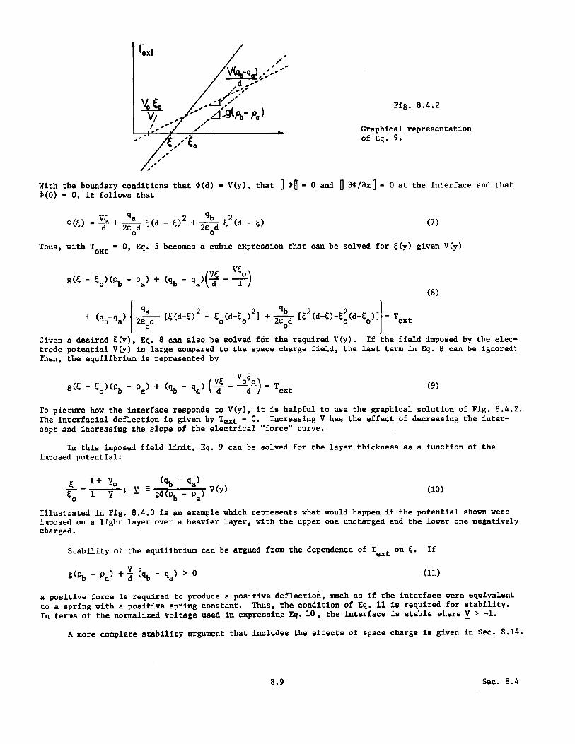
To picture how the interface responds to V(y), it is helpful to use the graphical solution of Fig. 8.4.2.

The interfacial deflection is given by Text = 0. Increasing V has the effect of decreasing the inter-

cept and increasing the slope of the electrical "force" curve.

In this imposed field limit, Eq. 9 can be solved for the layer thickness as a function of the

imposed potential:

S + Yo (qb - V() (10)0 1 gd(pb V(y)

Illustrated in Fig. 8.4.3 is an example which represents what would happen if the potential shown were

imposed on a light layer over a heavier layer, with the upper one uncharged and the lower one negativelycharged.

Stability of the equilibrium can be argued from the dependence of Text on C. If

g(Pb - ) + b - a) > 0 (11)

a positive force is required to produce a positive deflection, much as if the interface were equivalent

to a spring with a positive spring constant. Thus, the condition of Eq. 11 is required for stability.

In terms of the normalized voltage used in expressing Eq. 10, the interface is stable where V > -1.

A more complete stability argument that includes the effects of space charge is given in Sec. 8.14.

Sec. 8.4

V(qb-q),''

V_0 C Fig. 8.4.2

V 9- P-P)- / Graphical representation

0.5

V(y)1

-0.5

3

0

CY~cy

Uniform Current Density: Static equilibrium with the free-current force density Jf x poH dis-tributed throughout the volume of a fluid is now illustrated. In the MQS system of Fig. 8.4.4, a layer ofliquid metal rests on a rigid plane at x = 0 and has a depth ý(y). The system, including the fieldsand currents, is assumed to have a uniform distribution with the z direction, so that the view shownis any cross section.

The magnetic field is to be used in deforming the liquid interface. A d-c electromagnet producesa magnetic flux density with components in the x-y plane. In addition, a voltage source drives a uni-form current density Jo in the z direction throughout the fluid volume. This current density interactswith the imposed flux density to produce a vertical component of magnetic force in the liquid, and aresultant deformation of the interface. Note that because the fields are static, there are no surfacecurrents. Also, the liquid metal is not magnetizable, so there are no magnetization forces to consider.Finally, effects of surface tension are ignored. Therefore, the interface is in stress equilibrium,provided the pressure there is continuous.

The essential approximation in obtaining the irrotational force density throughout the volumeis that the imposed magnetic flux density is very large compared to the flux density induced by theimposed current density Jo. Thus, the force density takes the approximate form

t+4F = J i x [Bi + Bi ] (12)

The vector potential is convenient for dealing with B, because if the substitution is made B = V x A,then Eq. 12 becomes ? = -VC, wherein

9= -JoA(x,y) (13)

The imposed field approximation and the uniform imposed current result in the irrotational force densityrequired for static equilibrium. Given the particular field structure and the magnitude of the fieldexcitation, A(x,y) is known.

In an engineering application, the liquid metal might serve as a base for the casting of plasticor glass products.l The magnetic field can be controlled so that there is a ready means of alteringthe shape of the mold without a need for replacing the casting material. If a quiescent fluid state isdesirable, conditions for a static equilibrium are essential. From Eq. 8.2.3 and Eq. 13

p + pgx - J A = constant (14)

There is no current density in the gas above the interface, and hence no force density. The depthas y + -- is defined as E, and A (x = 5, y + -~o) is defined as A,. Then, Eq. 14 shows that for points

1. See U.S. Patent #3,496,736, "Sheet Glass Thickness Control Method and Apparatus," February 24,1970, M. Hurwitz and J. R. Melcher.

Sec. 8.4

Fig. 8.4.3

Imposed field equilibriumwith V = -0.7 sin(y).Shape of charge layer isgiven by Eq. 10.

8.10

Fig. 8.4.4. Layer of liquid-metal has the depth C(y) which is controlled by theinteraction of a uniform z-directed current density Jo and a magnetic fluxdensity induced by means of the magnetic structure.

(a) and (a') of Fig. 8.4.4

Pa' + Pag = Pa + Pag (15)

and for points (b) and (b')

Pb' + bg - JoA = P + Pbgb - JoA (16)

Because the hydrostatic pressures are the same at the primed and unprimed positions, subtraction ofEq. 15 from Eq. 16 gives a relation that can be solved for the height ý(y):

ý = ý6- Jo(A, - A)/g(p b - Pa ) (17)

The vector potential has the physical significance of being a flux linkage per unit length in thez direction. To see this, define X(y) as the flux linked by a loop having one edge outside the fieldregion to the right, the other edge at the position y and height C of the interface and unit depth inthe z direction. Then the flux linked per unit length is

S=Bnda = A.dk = Am - A(ý,y) (18)

and in terms of this flux, Eq. 18 becomes

o

g( bm - Pa) (19)

The flux passing through the interface to the right of a given point determines the depression at thatpoint. Proceeding from right to left, the flux is at first increasing, and hence the depression isincreasing. But near the middle, additions to the total flux reverse, and the net flux tends towardzero. Hence, ý returns to m?, as sketched in Fig. 8.4.4. Even if used only qualitatively, Eq. 19gives a picture of the interfacial deformation that is useful for engineering design. Measurementscan be used to determine X(x,y).

8.5 Potential and Flux Conserving Equilibria

Typical of EQS systems in which an electric pressure is used to shape the interface of a somewhatconducting liquid is that shown in Fig. 8.5.1a. Provided that the region between the cylindrical elec-trode and the liquid is highly insulating compared to the liquid, the interface is an equipotential.Because the applied voliage is constant and the equilibrium is static, this is true even for what mightbe regarded as relatively insulating liquids. Certainly water, molten glass, plasticizers and even

used transformer Oil will behave as equipotentials with air insulation between electrodes and interface.The liquid is in a reservoir. By virtue of its surface tension, the interface attaches to the reser-voir's edges at y = +4. Thus, continuity requires that the upward deflection of the interface underthe electrode be compensated by a downward deflection to either side. To be considered in this sectionis how the static laws make it possible to account for such requirements of mass conservation.

Secs. 8.4 & 8.58.11

In the MQS system of Fig. 8.5.1b, the liquid is probably a metal. To achieve the conditions fora static equilibrium, the driving flux source Fo is sinusoidally varying with a sufficiently highfrequency that the skin depth is small compared to dimensions of interest. Thus, the normal flux den-sity at the interface approaches zero. The liquid responds to the time average of the normal magneticstress.

IV•.

0'2 iN

Fig. 8.5.1. (a) EQS system; liquid interface stressed by d-c field is equipotential. (b) MQSsystem; driving current has sufficiently high frequency that currents are on surfaces ofliquid and electrode. Liquid responds to time average of magnetic pressure.

This pair of case Ptudies exemplifies the free charge and free current static equilibria, fromSec. 8.2, involving electromagnetic surface force densities. The EQS static equilibrium is possiblebecause there is no electric field tangential to the interface, while the MQS equilibrium resultsbecause there is essentially no normal magnetic flux density.

Antiduals: The two-dimensional fields in the two systems have an interesting relationship. Forthe moment, suppose that the geometry of the interfaces is known. Then, the electric field is repre-sented by the potential, while the magnetic flux density is represented in terms of the z componentof the vector potential, as summarized by Eqs. (a)-(c) of Table 2.18.1. Thus, in the regions betweenelectrodes and interfaces,

V2 4 = 0 V2A = 0

Boundary conditions on the respective systems are

= Vo on S

O f 0 on S2

A = F° on S1

A = 0 on S2

where S1 is the surface of the electrode or bus above the interface and S2 is the interface and ad-jacent surface of 1he container. By definition, Fo is the flux per unit length (in the z direction)passing between the bus and the interface. Note that to make the magnetic field tangential to thesesurfaces, A is constant on the interface and on the surface of the bus.

With the understanding that n denotes the direction normal to the local interface, the electricand magnetic stresses on the interfaces are

1 E2 1 e 2i€2nn 2 on 2 E n

1 2 1 1 A) 2

T = - pH = - Po nnn 2 0t 2 oU 3n

o

Thus, if the interface had the same geometry in the two configurations, the magnetic stress would "push"

Sec. 8.5 8.12

on the interface to the same degree that the electric stress would "pull." The magnetic stress is thenegative of the electric stress and can be formally found by replacing Co 4 Po and ac/In + (@A/Dn)/Vo.

Although limited to two-dimensional fields, the antiduality makes it possible to extend the elec-tromechanical description of one class of configurations to another by simply changing the sign of theelectromechanical coupling term. Provided that charge can relax sufficiently rapidly on the EQS inter-face to render it an equipotential even under dynamic conditions, and provided that motions remain slowcompared to the period of the sinusoidal excitation for the MQS system (so that the interface respondsprimarily to the time-average magnetic stress), the antiduality is valid for dynamic as well as staticinteractions.

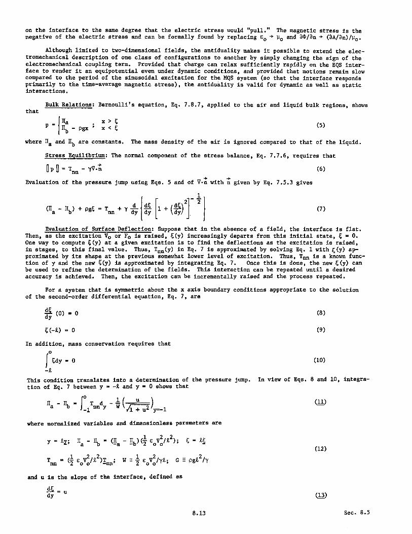
Bulk Relations: Bernoulli's equation, Eq. 7.8.7, applied to the air and liquid bulk regions, showthat

Ila x >Pi b - pgx x < (5)

where Ha and H1b are constants. The mass density of the air is ignored compared to that of the liquid.

Stress Equilibrium: The normal component of the stress balance, Eq. 7.7.6, requires that

p = Tnn- yV.n (6)

Evaluation of the pressure jump using Eqs. 5 and of V.n with n given by Eq. 7.5.3 gives

2] 2(IIH- ) + pgr= T + Y1+d(i )1[1+ (7)a b nn dy dy dyj

Evaluation of Surface Deflection: Suppose that in the absence of a field, the interface is flat.Then, as the excitation Vo or Fo is raised, ý(y) increasingly departs from this initial state, C = 0.One way to compute ý(y) at a given excitation is to find the deflections as the excitation is raised,in stages, to this final value. Thus, Tnn(y) in Eq. 7 is approximated by solving Eq. 1 with E(y) ap-proximated by its shape at the previous somewhat lower level of excitation. Thus, Tnn is a known func-tion of y and the new Q(y) is approximated by integrating Eq. 7. Once this is done, the new E(y) canbe used to refine the determination of the fields. This interaction can be repeated until a desiredaccuracy is achieved. Then, the excitation can be incrementally raised and the process repeated.

For a system that is symmetric about the x axis boundary conditions appropriate to the solutionof the second-order differential equation, Eq. 7, are

d- (0) = 0 (8)dy

(-E ) = 0 (9)

In addition, mass conservation requires that

jo dy =0 (10)

-P

This condition translates into a determination of the pressure jump. In view of Eqs. 8 and 10, integra-

tion of Eq. 7 between y = -k and y = 0 shows that

H- = Td1ny ( u (1)-a1an y W /+u y=-1

where normalized variables and dimensionless parameters are

y = y; a - b = (a - 4() oV2o/ 2) =((12)

T = (1 E V2/ 2 )T W - V2/y; G -pga2/

and u is the slope of the interface, defined as

dy ~

(

dy (13)

Sec. 8.58.13

In terms of u, Eq. 7 is normalized and written as a first-order differential equation

du (1 u2)3/2S(1 + u ) [(a - lb)W + Gý - WTnn] (14)

This last pair of relations, equivalent to Eq. 7, take a form that is convenient for numerical incegra-tion. (The integration of systems of first-order nonlinear equations, given "initial conditions," iscarried out using standard computer library subroutines. For example, in Fortran IV, see IMSL Integra-tion Package DEVREK.) With Tnn(y) given from the solution of Eqs. 1-3 (to be discussed shortly), theintegration begins at = -1 where Eq. 9 provides one boundary condition. To make a trial integrationof Eqs. 12 and 13, a trial value of u(-l) is assumed. Thus, from Eq. 11, the value of Ha-Hb that in-sures conservation of mass is determined. Integration of Eqs. 12 and 13 is then carried out and evalu--ated at y=0. Using u(-l) as a parameter, this process is repeated until the condition u(O) = 0 (bound-ary condition, Eq. 8) is satisfied. One way to close in on the appropriate value of u(-l) is by halvingthe separation of two u(-l)'s yielding opposite-signed slopes at y = 0.

Evaluation of Stress Distribution: To provide Tnn(y) at each step in the determination of thesurface deflection which has just been described, it is necessary to solve Eq. 1 using the boundary con-ditions of Eqs. 2 and 3. A numerical technique that is well suited to this task results in the directevaluation of the surface charge density af on the interface. Because Tnn = CoE2/2 = a2/2c , this istantamount to a direct determination of the desired stress distribution.

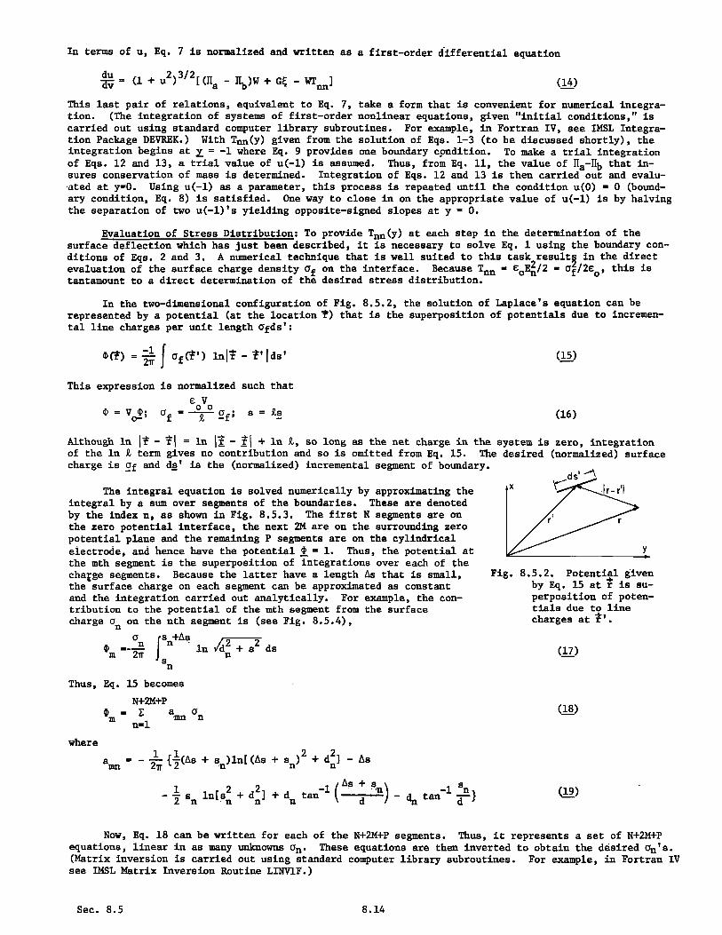
In the two-dimensional configuration of Fig. 8.5.2, the solution of Laplace's equation can berepresented by a potential (at the location t) that is the superposition of potentials due to incremen-tal line charges per unit length afds':

(15)(-1 afo ') Inj - t' ds'

This expression is normalized such that

EV4 = V4; a = ; s = (s

o- f Y f,

Although in 1 - fl = in - ( + In £, so long as the net charge in the system is zero, integration

of the In 1 term gives no contribution and so is omitted from Eq. 15. The desired (normalized) surface

charge is o and dg' is the (normalized) incrementa y

The integral equation is solved numerically by approximating theintegral by a sum over segments of the boundaries. These are denotedby the index n, as shown in Fig. 8.5.3. The first N segments are onthe zero potential interface, the next 2M are on the surrounding zeropotential plane and the remaining P segments are on the cylindricalelectrode, and hence have the potential 4 = 1. Thus, the potential atthe mth segment is the superposition of integrations over each of thecharge segments. Because the latter have a length As that is small,the surface charge on each segment can be approximated as constantand the integration carried out analytically. For example, the con-tribution to the potential of the mth segment from the surfacecharge ao on the nth segment is (see Fig. 8.5.4),n

a sn+AsSE n ns

m 27n

Thus, Eq. 15 becomes

In 2+ s2 dsn

Fig. 8.5.2. Potential givenby Eq. 15 at r is su-perposition of poten-tials due to linecharges at P'.

(17)

N+2M+P== a a

m n= mn nn=1

2 2a 1 (As + s )In[(A s + sn) + d - Asan 2'n 2 n n n

- 1 In[s 2 + d2 ] + d tan-l(As + ) - tan-1 sn2 n n n n d t

Now, Eq. 18 can be written for each of the N+2M+P segments. Thus, it represents a set of N+2M+Pequations, linear in as many unknowns an. These equations are then inverted to obtain the desired an's.(Matrix inversion is carried out using standard computer library subroutines. For example, in Fortran IV,see IMSL Matrix Inversion Routine LINVlF.)

Sec. 8.5

where

(18)

(19)

(16)

charve is a and ds'is-rthe noralied)incemenal e of

8.14

2Because T = a /2, the normalized stress distribution on each segment follows. So that the

-nn -nnumerical integration of the surface equations, Eqs. 13 and 14, can be carried out with an arbitrarystep size, the discrete representation of Tnn on the interface is conveniently converted to a smoothfunction by fitting a polynomial to the values of Tnn. (Polynomial fit can be carried out using a LeastSquare Polynomial Fit Routine such as the Math Library Routine LSFIT.)

m th segmentn th segment s

dn\\ -A-

Fig. 8.5.3. Definition of segments and geometry for Fig. 8.5.4. Typical segment on inter-numerical solution. face.

Typical results of the combined numerical integration to determine Tnn(y) and the interfacial de-formation are shown in Fig. 8.5.5. (These computations were carried out by Mr. Kent R. Davey.) Theprocedure begins with a modest value of W and a flat interface and starts with a determination of Tnn.Then, Eqs. 13 and 14 are integrated and this integration repeated until the boundary condition u(0) = 0is satisfied. Using this revised distribution of C(y), the distribution of Tnn is recalculated, followedby a recalculation of the interface shape. This process is repeated until a desired accuracy is achieved.

Fig. 8.5.5

Shape of interface withG = 3, r = 0.5 and h = 1.Broken culrves are for suc~-

cessive iterations l1) witnW fixed. (a) EQS systemwith W = 0.5. (b)MQS sys-tem with W = -0.5. Notethat electric case conver-ges monotonically, whilemagnetic one oscillates.

With W raised to a somewhat higher value, the previously determined shape is used as a startingpoint in repeating the iteration described.

Sec. 8.5

0.02

0

-0.02

Brokncrve areforsu-

8.15

HOMOGENEOUS BULK INTERACTIONS

8.6 Flux Conserving Continua and Propagation of Magnetic Shear Stress

Alfvyn waves that propagate along magnetic field lines in the bulk of a highly conducting fluidresult from the tendency for arbitrary fluid surfaces of fixed identity to conserve their flux linkage.The physical mechanisms involved are apparent in the one-dimensional motions of a uniformly conductingincompressible fluid permeated by an initially uniform magnetic field intensity Hoi , as in Fig. 8.6.1a.By assumption, each fluid particle in a y-z plane executes the same motion.

Y

(a) (b) (c)Fig. 8.6.1. (a)Perfectly conducting fluid initially at rest in uniform magnetic field.

(b) For flux conservation of loops of fixed identity initially lying in x-z planes,translation of layer in y-z plane requires induced currents shown. (c) Force den-sities associated with currents induced by initial motion. (d)Translation oflayers resolves into wave fronts propagating along magnetic field lines.

Consider the consequences of using an external force density Fexiy (Fig. 8.6.1b) to give ay-directed translation to a layer of fluid in one of these y-z planes. Because of the translation,fluid elements initially in any x-z plane form a surface that would be pierced twice by the initialfield Ho . It is shown in Sec. 6.2 that if the fluid is perfectly conducting, the total flux linkedby such a surface of fixed identity must be conserved. As a result of material deformation, a currentdensity (sketched in Fig. 8.6.1b) is induced in just such a way as to create the y component of mag-netic field required to maintain the net field tangential to each material surface initially in anx-y plane.

Note that because charge accumulation is inconsequential, the current density is solenoidal, sothat current in the z direction must be returned in the -z direction in adjacent planes. The forcedensity associated with these return currents is also shown in Fig. 8.6.1b. Because these currents areproportional to the displacement of a layer, the external force is retarded by a "spring-like" forceproportional to the magnitude of the displacement. Similarly, the returning currents in adjacent y-zlayers cause magnetic forces above and below, but here tending to carry these layers in the same direc-tion as the original displacement. Thus, fluid layers to either side tend to move in the same direc-tion as the layer subjected to the external force. Adjacent layers in the y-z planes are coupled bya magnetic shear stress representing the force associated with currents induced to preserve the con-stant flux condition.

In the absence of viscosity, the magnetic shear stress on adjacent layers is only retarded byinertia. There is some analogy to the viscous diffusion (Sec. 7.19), with the interplay betweenviscosity and inertia now replaced by one between magnetic field and inertia. The viscous shear stressof Sec. 7.19 is proportional to the shear-strain rate. By contrast, the magnetic shear stress in theperfect conductor is proportional to the shear strain (the spatial rate of change of the material dis-placement rather than velocity). Thus, rather than being diffusive in nature, the motion resultingfrom the magnetic shear stress in a perfect conductor is wave-like. As suggested by Fig. 8.6 .1c, themotion propagates along the lines of magnetic field intensity as a transverse electromechanical wave.Just how perfectly the fluid must conduct and how free of viscosity it must be to observe these wavesis now determined by a model that includes magnetic and viscous diffusion.

Sec. 8.6 8.16

A layer of fluid having conductivity 0, vis-cosity n and thickness A is shown in Fig. 8.6.2.In static equilibrium, it is permeated by a uni-form x directed magnetic field intensity Ho .Because the magnetic flux density is solenoidal,it is written in the form I = PHoIx + V x X, whereA is governed by the magnetic diffusion equation,Eq. 6.5.3. Fluid deformations that are now con-sidered are independent of z and confined to x-ylanes, and so only the z component of A exists;= AiZ . Moreover, motions are taken as inde-

pendent of y, so v = vy(x,t)iy and A = A(x,t).Thus,

1 D2A 3APo x2 = T + iHo y

xwhere[Eq.(b) of Table 2.18.1

where [Eq. (b) of Table 2.18.1]

(Av,)\

i.. .H--.----- --- L------

KVYV)Y

Fig. 8.6.2. Layer of liquid metal or plasmawith ambient magnetic field Ho .

1 aAy Iax

The fact that motions are independent of y and that I is solenoidal combine to show that Bx is inde-pendent of x, and hence Bx = ýHo even as the motion occurs. There is no linearization implied by thelast term of Eq. 1.

For the one-dimensional incompressible motions, conservation of mass is identically satisfied andonly the y component of the force equation is pertinent. With the magnetic stress substituted intoEq. 7.16.1, it follows from Eq. 2 that

2yv 2 A v

where the magnetic shear stress is T = pH H and the viscous shear stress is

vyxSyx =TD

The self-consistent coupling between field and fluid is expressed by Eqs. 1 and 3. Thesý repre-sent the one-dimensional response of the layer shown in Fig. 8.6.2. Given the amplitudes [la,A,v^ ,v]at the boundaries, what are the transfer relations for the amplitudes [H,HS x, S x] in these sameplanes? (Note that these relations are the limit k + 0 of more general transfer relations for travelingwave dependences on y. For the two-dimensional motions implied by such a dependence, vx becomes anadditional variable, and the normal stress Sxx is its complement. Thus, the more general two-dimensionaltransfer relations relate two potentials and four velocity components to two tangential fields and fourstress components, evaluated at the a and 8 surfaces.)

For complex amplitude solutions of the form A = Re A(x) exp(jwt), Eqs. 1 and 3 become differentiallaws for the x dependence:

2^1d v

S---• - jpy - H dA = 0

2 y 0 dx2

These constant coefficient expressions admit solutions A c exp(yx) and vy 0 exp(yx).that y must satisfy the relation (yA = y):

(y 2 - Jm ( v)

(Y _jWC m(Y _j WC V M=I

Substitution shows

(7)

Thus, the spatial distribution with x is determined by the magnetic diffusion time, Tm, the viscousdiffusion time, Tv, and the magneto-inertial time, TMI:

v MI o

Sec. 8.6

m

8.17

In the absence of the equilibrium magnetic field (Ho = 0), Eq. 7 shows that what remains is vis-cous diffusion (Secs. 7.18 and 7.19) and magnetic diffusion (Secs. 6.5 and 6.6). The parameter ex-pressing the coupling in Eq. 7, the ratio of the geometric mean of the magnetic and viscous diffusiontimes to the magneto-inertial time is defined as the Magnetic Hartmann number Hm = TmTv/TMIApHo0/O7. With the coupling, there are three characteristic times that determine the dynamics.

Even so, the biquartic form of Eq. 7 shows that there are still only four solutions to Eqs. 5and 6, y = ±71 and y = +y2 , where

1/2[21±~Y[H -- )2- + 2jW(T + Tv)H2

21

Thus, in terms of coefficients A1.* 4A,the solution is

A = A1 sinh Y1x + A2 sinh Y1 (x - A) + A3 sinh Y2x + A4 sinh Y 2 (x - A)

Equation 5 shows how to find vy in terms of these same four coefficients:

^ 1 /d2v = 2- jal-

y 2H 0 \dxo

(9)

(10)

(11)

Given the potential and velocity in the a and Rplanes, Eqs. 10 and 11 become four expressions that canbe inverted to determine A1 ... 4 . Fortunately, Al and A3 are determined by the a variables alone, andA2 and A4 by the 8 variables alone, so this task is not all that difficult. In fact, with a bit of hind-sight, the desired linear combination of solutions can be written by inspection:

{[ J 2•]~l sinh lx2 oy sinh 1

22jw )A 2 -]sinh Y1 (x-A)2 ovy sinh y1A

+ywc ,V U2Hasnhl + _sinhY2x + F Jw 1 ^+2 sinh y2(x-A)11 sinh Y 2)A 1 oHy sinh y22

Now, by use of Eqs. 11 and 12 in 2 and 4, the transfer relations follow:

= [Mij]

where with -k -YkA and qk = k - jW OA k = 1 or 2:

1(2

Ml(1) w -M2(2 - 2

2 1 l

cosh-1

Y21jsinh Y2 - Y2q1

cosh Y2sinh-1 sinh

,,oshy cosh Y2 Bi h YM1 (3) = -M2 (4 =- P H/0 2 2 -1 F

2 2 2 (-cosh

M23(l m M2H o d22 q12 1 sinh Y2 122p H A 2A Y

3(3) m -M4 (4) lq2 -1 sinh 71 --1q

2 2F = A(1 - Y2)sinh y1 sinh 72

Y) sixh -cosh

-/ 2•sinh Y1 1

2(cosh Y1 sinh Y /F

Sec. 8.6

(12)

2

(13)

Y]F/F

7I-/F

8.18

Temporal Modes: Suppose that the layer is excited in the a and 1 planes by perfectly conductingrigid boundaries that (perhaps by dint of a displacement in the y direction) provide excitations( ,). The perfect conductivity assures Aa = 0 and k = 0 (Eq. 6.7.6). Thus, the electrical andmechanical variables on the right in Eq. 13 are determined. The temporal modes for this system (thatrepresent the homogeneous response to initial conditions and underlie the driven response) are thengiven by F = 0. The roots of this equation are simply

Y1 = jnT; Y2 = jnT, n = 1,2,*.* (14)

With these values of y, Eq. 7 can be solved for the eigenfrequencies

S(n7 1 1 (n -+_ (15)n 2 T Tv 2 4

m v T m v

In the extreme where Tm and Tv are.long compared to TMI ,

nTn=+ (16)- TMI

This oscillatory natural frequency is the result of an Alfven wave resonating between the boundaries.The wave transit time is TMI = A/va, so va = VJHi/p is the velocity of this Alfv6n wave.

Typical of an experiment using a sodium-based liquid metal are the parameters

a = 106 mhos/m A = 0.1 m = 104 sec

3 3 -2S = 103 kg/m33H o = 1 tesla T = 1.25 x 10 sec (17)

2 -3n = 10-3 newton-sec/m2 M = 3.53 x 10- 3 sec

Thus, the characteristic times have the ordering TMI < Tm < Tv with the magnetic diffusion time farshorter than the viscous diffusion time. (The ratio of these times is sometimes defined as the mag-netic Prandtl number Pm = Tm/Tv = nrp/p. For the numbers given by Eq. 17, Pm = 1.25 x 10-6.) Thus,in Eq. 15, 1/Tv can be neglected compared to 1/Tm and it is seen that the natural frequency will dis-play an oscillatory part if

Tm nW> (18)TMI 2

That the transit time for the Alfvyn wave be short compared to the time for appreciable magnetic dif-fusion underscores the flux-conserving nature of the wave dynamics. For the numbers of Eq. 17,Tm/TMI = 3.54. As a practical matter, Alfv6n waves observed in the laboratory are relatively damped.Note that as A increases, the inequality of Eq. 18 is better satisfied. The dependence of the naturalfrequency on the mode number n reflects how damping increases with the wave number jy in the x direction.Near the origin in Fig. 8.6.3, the linear relation of frequency and mode number is typical of nondis-persive wave phenomena. As the mode number increases, magnetic (and possibly viscous) diffusion dampsthe oscillations, which then give way to totally damped modes. The oscillatory modes would of courseappear as resonances in the sinusoidal steady-state driven response.

Spatial Structure of Sinusoidal Steady-State Response: The penetration of a sinusoidal excitationfrom the surfaces into the bulk is determined by Y1 and Y2 , Eq. 9. As the magnetic field is raised,the viscous and magnetic skin effect are taken over by the electromechanical coupling. In Fig. 8.6.4,the transition of these complex wave numbers is shown, with the magnetic Hartmann number Hm representingthe magnetic field. In terms of characteristic times, Hm is increased until the magneto-inertial timebecomes sufficiently short that the Alfvyn wave can penetrate the layer before the flux diffuses to itsoriginal uniform distribution. The magnetic shear stress is then able to penetrate the layer (tendingto set the whole of it into motion) to a greater extent than would be possible via the magnetic orviscous diffusion alone. This is indicated by the lower of the roots shown, which has an imaginarypart Y + +,/mTv/AHn = +(TMI/A as Hm becomes large. In this same limit of large Hm, the other branchbecomes strongly decaying, with value y = +Hm/A. The physical nature of the dynamics represented bythis mode is recognized by observing that Hm -Tim/TMV, where TMV is the magneto-viscous time. Theelectrical analogue of this time, which expresses the rate at which a process occurs involving a compe-tion of viscous and magnetic stresses, will play an essential role in the next section. An experimentdemonstrating Alfvyn waves is sketched in Fig. 8.6.5.1

1. See also J. R. Melcher and E. P. Warren, "Demonstration of Magnetic Flux Constraints and a LumpedParameter Alfvyn Wave," IEEE Transactions on Education, Vol. E-8, Nos. 2 and 3, June-September,1965, pp. 41-47.

Sec. 8.68.19

Fig. 8.6.3. Eigenfrequencies of temporalmodes as a function of mode numberfor TMI = 0.0 1, Tm = 0.1, andTV = 1. wr - , i ------. m=31.6.

I

Y2 0

0 I 2HM ---------

Fig. 8.6.4. Real ( - ) and imaginary ( --- ) parts of71 and y2 (Eq. 9) as functions of Hm --AIHoIV7i.Low- and high-Hm approximations are shown. Notethat the Alfvyn wave branch is represented byjwrt-m'Tvm/v = jwrMI.

Fig. 8.6.5

Alfvyn wave, as demonstrated by Shercliffin film "Magnetohydrodynamics" (Reference 7,Appendix C). Liquid NaK (sodium-potassiumeutectic) fills conducting circular metalcontainer having coaxial inner and outerwalls. .Wave is excited at bottom by radialdriving current and detected at middle bycoil that senses the change in magneticfield accompanying the passage of the up-ward-propagating electromechanical wave.As viewed radially inward, layers of liquidmetal undergo shearing motions depicted byFig. 8.6.1.

8.7 Potential Conserving Continua and Electric Shear Stress Instability

In an electric counterpart to the magnetic flux conserving fluid introduced in Sec. 8.6, a fluidelement having fixed identity tends to retain its potential even as it moves. Under what physicalcircumstances could a homogeneous continuum tend to conserve its potential in this way? Figure 8.7.1gives a schematic illustration (see Prob. 5.12.1 for charge relaxation in anisotropic conductors).

Initially, the volume is filled with static layers of miscible fluid having the same mechanical

properties. Alternate layers are rendered conducting, perhaps by doping the same fluid as used for theother layers. At the upper and lower extremities, the conducting layers make electrical contact with

Secs. 8.6 & 8.7 8.20

X

rAYV V' VWV : W.

(a) (b) (c)Fig. 8.7.1. (a) Example of potential conserving fluid made from numerous conducting layers

buffered by relatively insulating layers. On a macroscale, a given fluid region tendsto retain its potential as it deforms. (b) Shearing displacement causing elevation ofpotential in plane (i) relative to that at the same position y in planes (ii) and (iii).(c) Charge density implied by potential conservation, showing electrical force in-duced by the motion in adjacent layers.

surfaces having a linear potential distribution in the y direction. Thus, there is an initialambient electric field I = Eo y throughout the volume. What would be termed an isotropic inhomo-geneous system on a microscale typified by the interlayer dimensions, is an anisotropic homogeneoussystem on the macroscale considered here. On this macroscale, a material element tends to retain itsinitial potential. In the model considered here, the conducting layers are of finite conductivity,but the layers between are considered perfect insulators. Just how faithfully the potential is con-served therefore depends on the electrical relaxation time of the composite.

By way of forming an intuitive impression of why the electric field induces instability, considermotions that are purely y-directed but depend on x. Suppose that the external force density Fexttv isused to translate a fluid layer in the y-z plane, denoted by (i) in Fig. 8.7.1b. To begin with, thepotential of this and the adjacent layers decreases linearly in the y direction. So, at a given posi-tion along the y axis, the translation results in the potential in the plane (i) becoming elevated withrespect to that of the adjacent layers (ii) and (iii). The adjacent layers form capacitor plates withthe (i) layer which, in accordance with the relative potentials, are charged as sketched in Fig. 8.7.1c.

The field- and deformation-induced charge of the initially displaced layer, (i), are such that it

is subject to an electrical force tending to further encourage the deformation. Thus, with the adjacent

layer fixed, the external force would act against a negative spring constant. However, the adjacent

layers are not fixed and experience electrical forces tending to carry them in a direction opposite

that of the original displacement. There is an electrical shear stress acting between adjacent layers

that is proportional to the negative of the strain. By contrast with the magnetic shear stress thatgives rise to Alfv6n waves, the electric stress tends to cause instability.

The laws needed to formulate a model begin with a constitutive law for the conduction. With n

defined as a unit normal to a material surface of fixed identity that is initially in an x-z plane,as shown in Fig. 8.7.1b, the component of the electric field that is tangential to this surface is

-x x t. Thus, if the average conductivity in the plane of the conducting layer is a, the currentdensity in a stationary sample of the anisotropic material is

J' = -ai x x (1)f

Because Jf = J~ + Pfv, it follows that the statement of charge conservation, Eq. 2.3.25a, is

xx + ] + = 0 (2)

+p~f ] t2

Sec. 8.7

E

0 i)i..-extni·,. + + + + + + fy

4++4+

(iii) \_

8.21

The normal vector can be eliminated from this expression by first expressing it in terms of the surfacey =f(x,t)

1

n = [i- i][l + ( )(3)

and then recognizing that because this surface is of fixed identity, the function F = y - 5 must have aconvective derivative that is zero (Sec. 7.5):

v =K-- + V (4)y =ft x ax

In Eq. 2, n can be replaced by Eq. 3, where E is in turn related to v by Eq. 4.

Before carrying out this elimination for the case at hand, note that because the electric field isirrotational and the perturbation quantities only depend on x, the electric field in the y direction isnot a function of x. Pinned at Eo in any y-z plane, Ey remains this value even as the fluid deforms:- = Eoty - (80/8x)x. As a result, Gauss' Law becomes

a2• pf•- -f-(5)2 Eax

The motions considered are only in the y direction: V = v (x,t). With this understanding,

Eqs. 2, 3 and 4 are linearized and combined to eliminate E, and Eq. 5 s substituted for pf, to obtain

2

- 2 [Ev --- (0 + -)] = 0 (6) -ax

This statement of the effect of the motion on the fields reduces to the linearized version of DO/Dt = 0

in the limit where the charge relaxation time, /a0, is short compared to times of interest. If thecharge can relax instantaneously, the potential of an element of fluid is conserved even as it deforms.

The y component of the force equation, Eq. 7.16.6 with V.' = 0 and Pex represented by the diver-gence of the stress tensor (given with Eq. 3.7.22 of Table 3.10.1), is

av 2 2v

p = -EE L + n - (7)at o ax 2 ax2

The x-component simply determines the pressure distribution required to equilibrate the x component ofthe electrical force density. Equations 6 and 7 represent the electromechanical coupling.

The quantity in brackets in Eq. 6 is zero throughout the volume when the fluid is in static equi-

librium. Hence, the two constants resulting from integrating Eq. 6 twice on x are zero. Then, withthe substitutions vy = Re y(x)ejwt and # = Re^(x)ejwt, Eqs. 6 and 7 become

Eo = j[1l + 1]$ = 0 (8)oy 0

2 2d d 0

(jwp - n 2 )v + CEo 2 = 0 (9)dx2)y dx

By contrast with the magnetohydrodynamic system represented by Eqs. 8.6.5 and 8.6.6, the system is only

second order in x, so that there are only two boundary conditions that can be imposed on a layer having

the thickness A (Fig. 8.6.2). Imposing a boundary condition on 0 is (through Eq. 8) tantamount to a

condition on vy. Substitution into Eqs. 8 and 9 of solutions having the form v = exp(yx) and 0 = exp(yx)gives a pair of homogeneous relations y

= 0 (10)2 2

jWp - ny SEoY

and the requirement that the determinant of the coefficients vanish gives an expression for the allowedvalues of y:

Sec. 8.7 8.22

Y = _Y1 Y1 2(11)

Tjn+w(l + a)

The situation is now no different than in dealing with Laplace's equation, where solutions take theform of Eq. 2.16.15 with y - y1. Thus, the transfer relation for the layer is (Table 2.16.1):

DB] -cosh(y 1A) 1

= le (12)Ssinh(Y 1 A) (12)

In terms of these variables, the mechanical variables follow from Eq. 8 as

v = [1 + _j (13)y E 1

o

dAA JITI [1 + q (14)

yx dx E 0 dx(o

Temporal Modes: Because the system is unstable, the temporal modes are of most interest. For asystem bounded by planes maintaining the linear equilibrium distribution in potential (constraigedA ozero pfrturbation potential), the condition on w resulting from there being a finite solution (Da,DO)with (Oa,$B) = 0 is sinh(y1A) = 0. Thus, the eigenvalues are

y1A jn'r, n = 1,2,3... (15)

The eigenfrequencies follow by substituting Y1 from this expression into Eq. 11. The result is a cubicequation which determines the allowed frequencies w:

3 2 [ (nr) 1 ( ] (n2)S- + - (2-(n2 = 0 (16)

2 T T T T TTVv v eo' EV E2

As a function of the mode number niT, the solutions sn = jW of this expression are illustrated inFig. 8.7.2. For each sinusoidal distribution represented by a given n, there are three temporalmodes, one unstable and two decaying.

Typical of a 2-cm liquid layer having 50 times the viscosity of water, the density of water,an electrical relaxation time of 10-2 sec and Eo = 2 x 10+5 V/m are the times given in the caption.Note that Te < TEV < TV .

The roots to Eq. 16 in the limit Te - 0 give a good idea of what is happening on time scaleslong compared to Te . The quadratic limit of Eq. 16 can then be solved to give

2 4Tvs = (w [-1 + + (17)

v EV(n )2

Thus, there are roots asn > 0 representing an exponentially growing instability. The fastest growingmodes are those having the largest number of wavelengths in the x direction. In the limit ni + m,this mode has a growth rate TEV. (In fact, there would be a finite mode exhibiting the maximum rateof growth, since wavelengths in the x direction shorter than the distance between layers are not de-scribed by the model.) By contrast with the electro-viscous nature of the short-wavelength insta-bility, the long wavelengths (small mode numbers) are electro-inertial in nature. In the limit nfr- 0,Eq. 17 reduces to sn = 1/TEI, where TEI = vTVEV = A/pEE2. Until its rate of decay becomes comparableto Te, the decaying mode can also be approximated using Eq. 17. At short wavelengths, the basicallyviscous diffusion mode and charge relaxation mode couple to produce a pair of modes that are damped ina sinusoidal fashion.

Sec. 8.78.23

S,

Fig. 8.7.2. Frequencies of temporal eigenmodes, sn = jw; --- (Sn)r, -- (sn)i.For each n there are three modes. Te = 10- 2 see, TEV = 0.1 sec, Tv = 10 sec.

The instability is fundamental to many situations where electric fields are used to augment mass,heat and momentum transfer. Usually a more complicated model is required even to recognize the linearstages of instability. Shown in Fig. 8.7.3 is an example for which the illustration given in this sec-tion is itself a useful model. The Couette mixer exploits a rotating inner cylinder to promote largescale mixing. Two liquids entering at the bottom are typically the highly viscous components of apolymer. Because of the rotation, these form laminae of relatively insulating and conducting liquidsthat work their way upward to the exit. With the application of a radial electric field, instabilityleads to mixing. The electrohydrodynamic instability provides mixing on a length scale that bridges thegap between what can be efficiently produced by the mechanical stirring and what is required to insure

Fig. 8.7.3

Couette mixer exploiting in-stability of componentsstressed by electric field.

ng

Sec. 8.7

i

8.24

genuine molecular scale mixing. 1 For successful operation the residence time of the liquids must atleast exceed TEV = n/cE2 . Even in its nonlinear stages and on length scales shorter than the distancebetween layers, TEV is found to scale the rate at which mixing processes occur." 3 In practical appli-cations, the "insulating" component actually is itself semi-insulating so the growth rate for instabilityis reduced by a factor reflecting the ratio of the component conductivities.

8.8 Magneto-Acoustic and Electro-Acoustic Waves

Electromechanical coupling through dilatational deformation is illustrated in this section.First considered as one-dimensional examples are perfectly conducting limits of the MQS and EQScontinua of Secs. 8.6 and 8.7, respectively. Then, the incremental motions of a system of magnet-izable particles randomly suspended in a uniform magnetic field are modeled.

Both the MQS and EQS configurations are shown in Fig. 8.8.1. Also shown in each case are the dis-tributed elements that embody the same physical phenomena as represented by the continuum models. With-out electromechanical coupling, the one-dimensional acoustic wave propagates through a continuum ofmasses (represented by the perfedtly conducting plates) interconnected by layers of fluid comprisingthe springs.

x• t)

H +h (Xt)OIzr~ l

/V

Eg ex(x,t)

fVx(x,t)

Z

Fig. 8.8.1. One-dimensional compressional motions. (a)Magneto-acoustic waves inperfectly conducting liquid across uniform magnetic field. (b) electro-acoustic waves in potential conserving continuum along uniform electric field.Lumped models emphasize salient features of dynamics.

In the magnetohydrodynamic case, the fluid is uniform and perfectly conducting. When at rest,it is permeated by a uniform magnetic field Ho directed transverse to the direction of propagation.Compression of the fluid results in a decrease in enclosed area for a contour such as C which isattached to the fluid. To retain the same flux linkage, a current is induced around this contour.The associated force density tends to counteract the dilatation, thus having the effect of a magneticspring between elements. It is not surprising that the magnetic field tends to increase the velocityof propagation of waves.

1. G. A. Rotz, "A Generalized Approach to Increased Mixing Efficiency for Viscous Liquids,"S.M. Thesis, Department of Mechanical Engineering, Massachusetts Institute of Technology,Cambridge, Mass., 1976.

2. J. H. Lang, J. F. Hoburg and J. R. Melcher, "Field Induced Mixing Across a Diaphragm," Phys.Fluids 19, 917 (1976).

3. J. F. Hoburg and J. R. Melcher, "Electrohydrodynamic Mixing and Instability Induced by CollinearFields and Conductivity Gradients," Phys. Fluids 20, 903 (1977).

Secs. 8.7 & 8.88.25

In the electrohydrodynamic case, a given element of fluid conserves its potential, as describedin Sec. 8.7. Either the fluid is a stratification of insulating and conducting components, or itactually consists of thin conducting sheets dispersed through the fluid. Because the motions are com-pressional, such sheets would not inhibit the motions. The equivalent distributed lumped parametersystem, shown in Fig. 8.7.1b, consists of perfectly conducting layers constrained to have the samepotential difference even as their relative spacing changes. As a "plate" approaches one of itsneighbors, the intervening electric field increases. So also does the electric force associated withthe charge on that side of the plate. Thus, the electric field is equivalent in its effect to a springwith a negative spring constant. It has the effect of diminishing the stiffness of the "spring"separating a pair of plates. The field is expected to reduce the velocity of a wave propagating in thex direction.

Now, consider the interactions in analytical terms. In both cases, the linearized longitudinalforce equation is simply

av a Tvx + xxPo at ax ax

where po is the equilibrium mass density, p' is the perturbation pressure, and Txx is the Maxwell stress.With the assumption that pressure is only a function of density, Eq. 7.11.3 can be used to replace theperturbation pressure with the perturbation density,

p' = a2p'

where a is the acoustic velocity. The permeability and permittivity in the respective situations aretaken as constant. Thus, with f and e the perturbations in A and t respectively, to linear terms,Txx becomes simply (Table 3.10.1, Eqs. 3.7.22 and 3.8.14)

T = (H +h )2 1 2H•2-_ohzxx 2 o z f o o0S1 2 1 2

Txx -E(E +e ) i CE oEoexxx 2 0 x 0 0ox

These last three equations combine to become

av ahx 2 2L z

o -t ax = o axavx 2 ex

o - + a2t- Eoax-

To linear terms, conservation of mass, Eq. 7.2.3, requires that

ap' Vxat + Po ax

These last two statements represent the mechanics, including the effect of the fields.

The reciprocal effects of the deformation on the fields follow from

the requirement that the flux linkedby a surface of fixed identity beconstant, Eq. 8.6.1. To linear terms

av ahx zH - =

oE 8xt

To combine these last three statements, take the time

Eqs. 5 and 6 and eliminate p and hz or ex:

a2vxa

at2

2Sav2 x

= am ax2

These wave equations make it clear that the effect ofwith a pagneto-acoustic velocity:

SH22 o

a = a +-m PO

the requirement that the potential,0, ofan element of fixed identity be constant,Eq. 8.7.1. To linear terms

,-Ev = 0

at ox

where e = -VO'x

derivative of Eq. 4 and the space derivative of

2avxx

at2

22 xe ax2

the fields is to replace the acoustic velocity

CE2 oa =Na -

e PO

Sec. 8.8 8.26

Acoustic velocities, given in Table .11.1, are typically 300 m/sec in gases and 1500 m/sec inliquids. In gases, the Alfvyn velocity, I/H~/po , can be made to dominate in its contribution to themagneto-acoustic velocity. In liquid metals the magnetic contribution to am is greatly reduced by theincreased mass density, although it is still possible for it to be significant. But in the electro-acoustic wave, electrical breakdown limits the effect of the electric field to a level that would makeit difficult to even measure the effect.

Magnetization Dilatational Waves: Although electromechanical effects on dilatational motions innatural materials are likely to be small, continua formed from "molecules" that are actually macro-scopic in their dimensions can give rise to significant electromechanical effects. As an example, mag-netizable spheres are suspended in a random array, with the voidage a gas or even vacuum. Interest isconfined to deformations characterized by lengths that are large compared to the distance between par-ticles. Unperturbed, the system is uniform on the macroscopic scale, and is subjected to a uniformz-directed magnetic field intensity Ho . Because the spheres can interact with each other only throughthe magnetic field, the pressure is taken as zero.

Perhaps determined experimentally, the effective permeability of the continuum has been relatedto the mass density through a constitutive law, i = 1(p). Thus, the force density of Eq. 3.8.17 from

Table 3.10.1 is applicable. With perturbations from the equilibrium mass density and magnetic field,

Po and Holz, denoted by p' and i, respectively, this force density is linearized to become

2=PoV[Ho(h)ohz + H 2 ) (9)

Because there are no free currents, Itis irrotational and hence H = H 1 - Vi. Thus, the force equation,Eq. 7.4.4 written with p = 0, is

÷ Po 2p -=opH()oV(- ) + -o H( )oVP' (10)Po at 0 0 o z 2 o=2 o

Mass conservation is represented by a linearized version of Eq. 7.2.3:

50 + poV. = 0 (11)t o

In terms of the scalar potential, 4, the linearized statement that pH is solenoidal is

-P(po ) V2 ý + Ho o = 0 (12)

To obtain an expression for p' alone, the divergence of Eq. 10 is taken. Then Eq. 11 eliminates V-v,while the D( )/Dz of Eq. 12 can be used to eliminate P. Thus, the expressions combine to give

22p poH2 2 P, 2 (13)

2 t H2(-3)VHp' (13)t2 (po ) o z 2 2 o 20

A possible relation between permeability and mass density is the Clausius-Mossotti law:1

(--- - 1)(P- P) 2 2p= C 3 + 2)( 1 ) p- 1 _ = ( 1) 2)p - 2 (14)

(-~ 2) 0oo p2 9 o

where C is determined by the nature of the spheres.

It follows from Eqs. 13 and 14 that compressional motions across the field lines (in the x direc-tion) are unstable, while those in the direction of the field propagate with the velocity

H 2 P P 1 2 LoaM =( + 2)( - 1) (15)

1. J. A. Stratton, Electromagnetic Theory, McGraw-Hill Book Company, New York, 1941, p. 140.

Sec. 8.88.27

PIECEWISE HOMOGENEOUS SYSTEMS

8.9 Gravity-Capillary Dynamics

The incompressible dynamics of fluids that are inhomogeneous in mass density are as commonplaceas wave motions in a teacup or at the interface between sea and atmosphere. At the interface, themass density suffers a step discontinuity. Fundamentally, the pertinent laws express the fact thatthe mass density in the neighborhood of a particle of fixed identity remains constant, Eq. 7.2.4, thatmass is conserved, Eq. 7.2.5, and that inertial and pressure forces balance. For the present purposesthe fluid is represented as being inviscid, and hence the pertinent force law is Eq. 7.4.4 with theexternal force density that due to gravity, f = p1.

ex

Because inhomogeneities in electrical properties are often accompanied by variations in mass den-sity, electromechanical interactions with inhomogeneous systems are commonly interwoven with the fluidmechanics resulting from effects of gravity. In this section, the mechanics of a fluid interfaceillustrates effects of gravity in systems that are inhomogeneous in mass density. If the interface isbetween immiscible fluids, effects of capillarity are also important.

In the configuration shown in Fig. 8.9.1, planar layers of fluid each have uniform propertiesdesignated by the subscripts "a" (above) and "b" (below), respectively, and a common interface atx = C(y,z,t). The lower fluid rests on a rigid boundary while the upper one consists of a deformablestructure. The system is driven from this structure by the traveling-wave excitation shown in thefigure. What is the response of the fluids, and in particular of their interface?

(C)Ra k,z)

(d)--(e)r_7 ..

Fig. 8.9.1. Fluids of differing mass densities have interface at 5and are driven by structure at E.

In the absence of the excitation, the fluids are in static equilibrium with the gravitationalforce density. Thus, the fluid velocity v = 0 and the pressure balances the gravitational force den-

sity. From the force equation, Eq. 7.8.3, applied to each region:

p =-Pagx + Ha; x > 0p = (1)

-pb g x + Hb; x < 0

Perturbations from this static equilibrium are represented in terms of complex amplitudes. Tolinear terms the pressure and velocity are

p = -pgx + H + p'(x,y,z,t); p' = Rep(x)exp j(wt-k y - kzz) (2)

= Rev(x)exp j(wt - kyy - kzz) (3)

Within a given fluid region the mass density is uniform. Thus, the complex amplitudes in the respective

planes designated in Fig. 8.9.1 are related by the transfer relations for an inviscid fluid given by

Eq. (c) of Table 7.9.1:

^C-coth(ka) 1 c ^ep -coth(ka) sinh(ka) x p -coth(kb) 1 ^eJap a JwPb sinh(kb) x

k k (4)^d -1 cd ^f

sinh(ka) coth(ka) P -i csinh(ka) sinh(kb) coth(kb) vJ

Sec. 8.9

X

8.28

Complex amplitudes are evaluated in the equilibrium planes. But, the jump conditions apply wherever theinterface is actually located and that location is in fact yet to be determined! This difficulty issidestepped by linearizing the jump conditions in such a way that they are expressed in terms of per-turbation variables evaluated at the equilibrium positions of the boundaries.

Taking boundary and jump conditions from top to bottom, observe first that the position of thedeformable upper structure is related to the velocity of the adjacent fluid by Eq. 7.5.5, which to linearterms is

vc = j~ (5)X

where it is appropriate to use the complex amplitude evaluated at the equilibrium position because thedifference between that and A (x = a + E) is second order in the perturbation amplitude, E.

Similarly, at the interface the velocities are related to the interfacial deformation by

^d ^ Ae

vx = JW; v = jW (6)

Again, this jump condition, which expresses mass conservation for the interface, has been written interms of amplitudes evaluated at the equilibrium interfacial position. Stress balance for the inter-face is represented by Eq. 7.7.6, which has only a normal component. To linear terms, this is repre-sented by the i = x component

[-a + a Pd(x=)]-[-Pb +b e(x=)] = 2 + ) (72

where the surface tension force density is given by Eq. (c) of Table 7.6.1. For static equilibrium,

Ha-Hb = 0. Also, to linear terms the perturbation pressures evaluated at the perturbed position E areequal to these pressures evaluated at the equilibrium position of the interface. Thus, Eq. 7 reducesto

Ad A 2Ad e (Pa - Pb) - yk E (8)

It is because the fluid is inviscid that the other two components of the interfacial stress balanceequation are, to linear terms, identically satisfied. Finally, on the rigid lower boundary

v = 0 (9)

The boundary and jump conditions, Eqs. 5, 6, 8 and 9, are now used to "splice" together the bulksolutions reýresented by Eqs. 4. Of the four equations summarized by these relations, the expressionsfor Dc and F simply serve to determine these pressures once the fluid motions have been determined.The other two, Eqs. 4b and 4d, are evaluated using the boundary conditions, Eqs. 6, 7 and 10, and sub-stituted into the stress balance condition, Eq. 9, to obtain

2 2W2 A 2 A W 2

- - [pa coth(ka) + pb coth(kb)]+ + [yk+ g(P - a ) = k sinh(ka) (10)

This relation has the same form as would be used to describe the deflections of a spring attachedto a mass at one end and to a displacement source at the other. The "mass" reflects the inertia of thefluids to either side of the interface while the "spring" results from the combined gravitational andcapillary forces.

From Eq. 10, it follows that the complex amplitude of the interfacial response is

2225 - a (11)

k sinh(ka) D(w,k)

where the dispersion equation, D(w,k), is

D(W,k) [P= coth(ka) + p coth(kb)] + [k 2 g(Pb - Pa)] (12)

Driven Response: The response having the same wave number and frequency as the drive would repre-sent all of the motions if the system were reentrant in the direction of the traveling wave and suf-ficient time had elapsed for a temporal sinusoidal state to be established. (This presumes that thetemporal natural modes are stable.) Under the assumption that yk2+g(pb - Pa) > 0 (which is assuredregardless of wavelength if the lower fluid is the heavier), the frequency response of the interface isas shown in Fig. 8.9.2. Because there are no dissipation mechanisms included in the model, the inter-face is either in phase or 1800 out of phase with the excitation.

8.29 Sec. 8.9

Gravity-Capillary Waves: The resonance comes

at that frequency that gives synchronism between

the hase velocit /k of the drive and hase

velocity of a gravity-capillary wave propagatingon the interface. Solution for w/k of Eq. 13set equal to zero identifies the phase velocityof these waves as

yk + g(pb - Pa)/kv (13)p Pa coth(ka) + pb coth(kb)

Long waves are dominated by gravity whileshort ones are of a capillary nature. Often,the waves are short enough that effects of thetransverse boundaries are not significant,laki >> IbkI >> 1. Then, Eq. 13 reduces to

vk g(Pb- Pa+= + + (14)_P Pa + b k(pb + Pa

This makes it evident that there is a wavenumber for minimum phase velocity, found bysetting the derivative with respect to k ofEq. 14 equal to zero. The wavelength, 2W/k,of this minimum will be termed the Taylorwavelength, AT:

I m 2., (1;)T - "g(pb - Pa) -

At wavelengths longer than AT, gravity wavesprevail, while shorter wavelengths represent Fig. 8.9.2. Driven response of gravity-capillary ripples. For an air-water interface, capillary wave system.

AT = 1.7 cm.

In the opposite limit of long waves, Ikal << 1 and Ikbl << 1, the phase velocity becomes

2Yk + g(Pb - Pa)

v = • a ( (16)p [(Pa/a) + (pb/b)

and the gravity wave (which is likely to dominate in a long-wave situation) propagates without dis-persion. A quasi-one-dimensional model for long gravity waves results in the wave equation with avelocity given by Eq. 16 without the capillary term.

Temporal Eigenmodes and Rayleigh-Taylor Instability: Temporal transients, initiated from conditionsthat are periodic in the horizontal plane, are described by D(w,k) = 0 with k real and jw the eigenfre-

quencies sn . The role of the temporal modes in this chapter is very much as introduced in Sec. 5.15.

The roots of D(sn,k) = 0 are either purely real or imaginary. Resonance in the driven response results

from the coincidence of the natural frequency and the driving frequency. Of most interest is the in-

stability resulting from having the heavier fluid on top and sufficiently long wavelengths that

yk2 < g(Pa -b) (17)

Note that this condition prevails for wavelengths longer than the Taylor wavelength defined with Eq. 15.

The eigenfrequencies can be pictured as poles in the complex s plane, with the density difference Pb-Paa variable parameter. For Pb > Pa, the poles are conjugates on the imaginary axis. With decreasingdensity difference and long enough wavelength, the poles migrate to the origin, and as the condition ofEq. 17 prevails, the poles separate on the real axis. The instability is incipient at zero frequency.In general, there might be an infinite set of eigenfrequencies. If all pass into the right-half s plane

through the origin, the principle of exchange of stabilities applies. That is, the incipient conditioncould be identified by setting w = 0 at the outset and asking for the condition on pb - P that makesit possible for all of the fluid mechanics laws to be satisfied. Here, as in Sec. 5.15 where thecharge relaxation eigenfrequencies for a step discontinuity in electrical properties is considered, thereare a finite number of eigenfrequencies (two). There it is shown that a smooth distribution of elec-trical properties leads to an infinite set of temporal modes. It should come as no surprise that asmoothly distributed density distribution similarly leads to an infinite set of eigenmodes. In that case,taken up in Sec. 8.18, the principle of exchange of stabilities also applies.

Sec. 8.9 8.30

...'.: Corn.. oil

Fig. 8.9.3a. Heavy liquid is stabilized on topof lighter fluid by means of polarizationforces induced by applying potential dif­ference to the diverging glass plates.These plates have a thin transparentcoating that renders them conducting.

The inviscid model is especially justified for predicting the incipience, because there are thenno temporal rates involved. Thus the effects of viscosity vanish.

1In the example of this Rayleigh-Taylor instability shown in Fig. 8.9.3, polarization forces are

used to stabilize a static equilibrium with a heavy liquid on top of a lighter one. (The electro­mechanics is developed in Sec. 8.11.) When the field is removed, the unstable temporal eigenmode isevident. Some fluid rises so that some can fall. The sinusoidal deflection predicted by the lineartheory gives way to a plume extending into the lighter liquid. It is characteristic of this purelymechanical instability that the nonlinear "process" initiated by the instability becomes blunted in itsadvanced stages. The bulbous plume can itself be unstable if the viscosity is low. This characteristicappearance, which is cOUDllonly seen "upside down" as warm air rises into the atmosphere, is in sharpcontrast with the electromechanical forms of Rayleigh-Taylor instability considered in the followingsections.

Spatial Eigenmodes: Spatial modes are introduced in Sec. 5.17. With longitudinal boundary condi­tions, the sinusoidal steady-state response consists not only of a part having the same wave number asthe transverse drive, but an infinite set of eigenmodes having the same frequency as the drive, eachwith its own wave number. These are in general complex, k = k + jki' and found by solving the disper­sion equation D(w,k) = 0 for k, given that W is the same as fo? the drive. In general this expressionis transcendental, so that it must be solved numerically. Here, an infinite set of eigenvalues can beidentified by a simple graphical solution. First, there are the two propagating modes in which k = kand the dispersion equation becomes r

(18)

A graphical solution is obtained by finding the intersection of curves representing the right and leftsides of this expression as a function of (a~). This is shown in Fig. 8.9.4a. An infinite set ofmodes are evanescent, k = jki • With k purely imaginary, the dispersion equation is again purely real(coth jx = -j cot x):

2[yki - g(Pb - Pa)]kiw2 = (19)

Pa cot(kia) + Pb cot(kib)

so that graphical solution gives rise to an infinite set of kits, as illustrated in Fig. 8.9.4b. Thefunctions on the right in these last two expressions are even in the wave number, so for each positiveroot there is a negative one as well. The two propagating modes have an exponential dependence on depth,while the evanescent modes are sinusoidal in their depth dependence, with a number of zero crossings inthe x direction that increases with the mode number.

1. See J. R. Melcher and M. Hurwitz, "Gradient Stabilization of Electrohydrodynamically Oriented Liq­uids," J. Spacecraft and Rockets~, 864-881 (1967).

8.31 Sec. 8.9

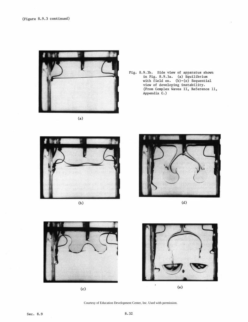
(Figure 8.9.3 continued)

Fig. 8.9.3b. Side view of apparatus shown in Fig. 8.9.3a. (a) Equilibrium with field on. (b)-(e) Sequential view of developing instability. (From Complex Waves II, Reference 11, Appendix C.)

(a)

(b) (d)

(c) (e)

Sec. 8.9 8.32

Courtesy of Education Development Center, Inc. Used with permission.

Fig. 8.9.4

Graphical solution for spatialeigenmodes. (a) Equation 18for propagating modes.(b) Equation 19 for evanescentmodes. For case shown, Pa = 0and Y/pbga2 = 1.

(a) (b)As an example, a gravity-capillary resonator might be constructed with rigid walls in the planes

y = 0 and y = )y and z = 0 and z = Zz. These propagating and evanescent modes would in general also beexcited by the transverse drive. In general, the evanescent modes are required to insure there beingno normal velocity on the longitudinal boundaries. With the surface tension comes still another bound-ary condition. For example, by virtue of the surface tension, the interface can cling to a sharp edge.Note that for Pb > Pa the lowest evanescent mode in fact exists because of the surface tension. Itrepresents the effect of the surface tension reaching out into the interfacial region from the longi-tudinal boundary. The higher order modes are more closely connected with the inertia and mass conserva-tion represented by Laplace's equation in the fluid bulk.

8.10 Self-Field Interfacial Instabilities

If a magnet is held over or under the free surface of a ferrofluid so that the field is normal to

the interface, sprouts of liquid will be seen to extend into the air. With the magnet fixed, the sprouts

are fixed. Even if stressed by an initially perfectly uniform magnetic field (so that hydrostatic pres-

sure can balance the magnetic forces to maintain a static equilibrium with the interface flat), the

sprouts represent a new static equilibrium preferred by the fluid. The electromechanical form of

Rayleigh-Taylor instability that takes place as the planar interface, stressed by a uniform magnetic

field, gives way to the new configuration, is one of the results from the model now developed. The con-

figuration, shown in Fig. 8.10.1a, consists of planar layers having different permeabilities (Ia,Pb),mass densities (Pa,Pb) and equilibrium thicknesses (a,b). The common interface is at x = ý, while rigid

boundaries (infinitely permeable pole faces) bound the layers from above and below. The liquids are

water based or even hydrocarbon based ferrofluids. Hence, in MQS terms, the materials are essentiallyinsulating. Only the magnetization force density, Eq. 3.8.14 with if = 0, is responsible for the elec-

tromechanical coupling.Av

- -ReiFe j(wt- kyy - kz z ))opooon0 ooro)nooono'

S(c)

a [LaP a B0~___~l_'M

- .. (f): :. .Eb :Pb

(a) (b)Fig. 8.10.1. (a) Layers of magnetizable fluid are stressed by a uniform normal

magnetic flux density, Bo . Polarizable liquid layers are stressed by anormal electric displacement, Do .

-V-ReVeiJ(wt-kyy-kzz )

Sa, Pa Do

Secs. 8.9 & 8.108.33

The time and space-varying drive is taken as imposed on the upper transverse boundary by means ofa coil structure. Thus, the magnetic potential in this surface is an equilibrium value -Co(relative A

to the lower surface) representing the magnet field plus a traveling wave having the complex amplitudecF

The EQS system, consisting of layers of insulating polarizable fluid as shown in Fig. 8.10.1b, isdescribed with the same model by simply identifying 1 + e, Bo 4 Do andý /r. There is an importantphysical difference between the two systems. To obtain a purely polarization coupling, it is necessaryto use an alternating electric field having a high enough frequency to guarantee that free charge doesnot enter into the electromechanics. This field can be considered as being essentially static providedthe frequency is also high enough to insure that the fluid responds to its rms value. In the respectiveregions the magnetic field is taken as having the form of an equilibrium plus a perturbation:

= x-VT (1)

The equilibrium magnetic flux density in each region is related to the equilibrium magnetic potentialdifference between the pole faces by

B =1IH = 0-/o (2)o a a =bHbA [(a/ua) + (b/jb)]

The magnetization force density is confined to the interface, where it acts on the equilibriuminterface as a normal surface force density. The equilibrium pressure difference Ha - Eb then holdsthe interface in static equilibrium. In the bulk regions, the magnetic field is uncoupled from thefluid nechanics. Thus, the perturbation mechanics of each layer is described by the inviscid pressure-velocity relations from Table 7.9.1, Eqs. 8.9.4. Similarly, the perturbation magnetic field is de-scribed by the flux-potential transfer relations, Eqs. (a) of Table 2.16.1 (k ' k+ k2)

-coth(ka) 1sinh(ka)

-1sinh(ka) coth(ka)

sinh(ka)

Ac

AdT4

hex

^fhx

=k

1-coth(kb) sinh(b)

sinh(kb)

-1coth(kb)

sinh(kb)

The essence of the electromechanics is in the boundary conditions, which must be consistent withthe electromagnetic and mechanical laws used in the model. Proceeding from top to bottom inFig. 8.10.1a, the magnetic potential must be that of the drive at the upper boundary. The boundary isrigid, so

T =• (4)

v = 0 (5)x

At the interface, continuity requires that

^d ^ev = v = j (6)x x

The x component of the stress balance jump condition, Eq. 7.7.3, is to linear terms equivalent to thenormal component of the stress balance. With i = x, that jump condition is evaluated using the stresstensor with Eq. 3.8.14 in Table 3.10.1:

[-Pagx + Ha d,d - [-Pbgx + Rb + Pe]x= (7)

[1i (Ha + d 1i 22 +2+1 T14b(Hbdh) 2 x= +Y( 42 )a22 a (Ha + hd) 11b (Hb + hx+ 2 x=

where, remember, all quantities are evaluated at the actual position of the interface. The normal

vector is written in terms of 5 by means of Eq. (a) from Table 7.6.1. Terms from the stress that are

nonlinear in the perturbation amplitudes have already been dropped in writing Eq. 7. To linear terms,the perturbation quantities evaluated at x = ý are the same as if evaluated at the equilibrium inter-

facial position x = 0. Also, the equilibrium magnetic field is uniform (not a function of x like the

equilibrium pressure), so these terms are the same at x = 0 as at x = 5. The equilibrium part of

Eq. 7 expresses the condition for static equilibrium,

Ea - Hb =(aH - H = B (Ha -

chx

^dhx

= k

Ae

^f

T

(3)

Sec. 8.10 8.34

and the perturbation part becomes the required jump condition representing stress balance at the inter-face:

(d _ e) g(0b Pa ) = Bo x - h - k(9)

The conditions of Eqs. 6 and 9 guarantee that the mechanical laws are satisfied through the interface.Similarly, on the magnetic side, ý is irrotational and ý is solenoidal, so x* = 0 and *. ElP = 0(Eqs. 21 and 22 of Table 2.10.1). With n again given by Eq. (a) of Table 7.6.1, either the y or z com-ponents of the condition that tangential ý be continuous reduces to

•d- e = (Ha - Hb) (10)

while the continuity of normal flux density is to linear terms given by

^d = ^eIah = bh (11)ax b x

Finally, there are the mechanical and magnetic conditions at the lower rigid and infinitely permeableboundary:

^fv = 0 (12)

Y = 0 (13)

With the objective of finding the driven response and in the process deducing the dispersionequation, the stress and field continuity conditions, Eqs. 9, 10 and ll,are now written with the p'sand hx's substituted from the bulk equations, Eqs. 8.9.4 and 3. These latter relations are themselvesfirst written using the remaining simple boundary conditions. Thus, Eqs. 9, 10 and 11 respectivelybecome

2

k [pacoth(ka) + Pbcoth(kb) - g(pb-P)-k2y kB coth(ka) kB coth(kb)

Ha - Hb - +1

0 akcoth(ka) Vbkcoth(kb)

Ad

Ae

^ k

sinh(ka)

0

sinh(ka)

Lsinh (ka)

(14)

Solution for Z gives

kBo(N - Pa)coth(kb)~ 1

sinh(ka)[ýbcoth(kb) + iacoth(ka)] D(w,k) (15)

where2

D(w,k) =- [Pacoth(ka) + pbcoth(kb)] + [Yk 2 + g(b akBa(bb - aa)

-- (16)allb ibtanh(ka) + Vatanh(kb)]

The many types of information that can be gleened from Eq. 15 are illustrated in Sec. 8.9. Con-

cerning the driven response, it is here simply observed that its frequency dependence is similar to

that illustrated by Fig. 8.9.2, with the frequency of the resonance occurring as the excitation phasevelocity coincides with that of a field coupled surface wave having the phase velocity

yk + g(b-Pba)/k - B(b-2a)2 /ab[ btanh(ka) + tanh(kb)] (17)

v pacoth(ka) + pbcoth(kb)

The -effect of the field is to reduce the gravity-capillary phase velocity and hence the frequency. This

phenomenon is a "self-field" effect, in the sense that a deformation of the interface distorts the mag-

netic field and this in turn creates a magnetization perturbation surface force density that tends to

further increase the deflection.1

1. For experimental documentation of resonance frequency shift with magnetic field, see R. E. Zelazo

and J. R. Melcher, "Dynamics and Stability of Ferrofluids: Surface Interactions," J. Fluid Mech.

39, 1 (1969).

8.35 Sec. 8.10

The tendency for this self-field coupling to precipitate instability makes the temporal modes ofK particular interest. In the short-wave limit ka << 1 and kb << 1, solution of the dispersion equation

D(w,k) = 0 for w2 results in

2 gk(Pb - Pa ) k3 k2B2(b - a)Pa + b + (Pa +P, + Pb Pa + Pb ýalb(pa + Pb)(Pa + Pb)

(18)

Even with the lighter fluid on top (say air over a ferroliquid) so Pb > Pa, the magnetic field can make2 -+ 0 and hence one of the eigenmodes unstable. Figure 8.10.2 shows W 2 as givenby Eq. 18 as a func-tion of k. As Bo is raised, there is a critical value at which the curve just kisses the w2 = 0 axis.Under this condition, instability impends at the wave number k . For greater values of Bo, wave numbers

between the roots of Eq. 18 with W2 = 0, ku and kk, are unstable. These roots coalesce as the dis-criminant of the quadratic formula vanishes. Thus, the incipient condition is

o(b a)

Pa1 b ta bb)y(19)

4g(p b - a)

Y

The critical wave number is what remains from the quadratic formula, which in view of Eq. 19 is

Sg(- a (20)k = (20)

Fig. 8.10.2

Dependence of w (k) as given byEq. 18 with B2 as a parameter.

0

r • •7

Note that the first perturbations to become unstable as thehave the Taylor wavelength given by Eq. 15.2

field reaches the level predicted by Eq. 19

What happens if the field is raised above the value consistent with Eq. 19? The initial rate ofgrowth is given by the linear theory, although because a rate process is now involved, this may bestrongly influenced by the viscosity. But, the ultimate state will depend on the nature of the electro-mechanical coupling. In the magnetization example at hand, the interface typically reaches a new stateof static equilibrium. The protrusions shown in Fig. 8.10.3 are typical. Consistent with the factthat the interface is always free of a shearing surface force density, they are perfectly static.

As discussed in the introduction to this section, to obtain a similar instability in the EQS polari-zation configuration of Fig. 8.10.1b, it is usually necessary to use an alternating field.3 If the fre-quency of this field is low enough that the natural modes can interact with its pulsating component, para-metric instabilities can also result. By contrast with the coupling described here, these instabilities

2. Conditions for instability are studied by M. D. Cowley and R. E. Rosensweig, J. Fluid Mech. 30,721 (1969).

3. E. B. Devitt and J. R. Melcher, "Surface Electrohydrodynamics with High-Frequency Fields," Phys.Fluids 8, 1193 (1965).

Sec. 8.10

I

8.36

aJu_

E

.. 0-." '., ... '. -:. '. . ~.....<:

1v.;

Fig. 8.10.4. Rigid plane-parallel electrodesbound liquids having common interface.The upper liquid is insulating relativeto the lower one.

Fig. 8.10.3. System of static fluid sprouts repre­sents a new static equilibrium formed onceplanar interface in perpendicular fieldbecomes unstable. (Courtesy of FerrofluidicsCorp., Burlington, Mass.)

are dynamic in character and can result in splattering or atomization of the interface. 4

To appreciate the perfectly static equilibrium of the polarization sprouts resulting from the in­stability of the flat interface, consider by contrast some of the possibilities resulting when the inter­face of a conducting fluid bounded by a relatively insulating one is stressed by a normal electric fieldEo' The configuration is shown in Fig. 8.10.4. For example, the upper fluid might be air and the lowerone water (or any other liquid having a charge relaxation time E/cr short compared to times of interest).5

The boundary condition at the interface is thatit sustains no tangential electric field. This isformally equivalent to the (analogous) magnetic fieldsituation in the limit where the lower fluid is infini­tely permeable. That is, in the limit ~b + 00, theinterfacial tangential magnetic field just above theinterface of Fig. 8.l0.la must vanish. The magneticfield above this infinitely permeable fluid thensatisfies the same boundary conditions as the elec­tric field does in the physically very differentsituation of Fig. 8.10.4.

It follows from Eq. 19 with the substitution~~ + E, ~b + 00 and Bo + Eo/E =~a that the volt­age required to just induce instability of theinterface is

8.10.5. Nonlinear stages of surfaceinstability caused by applying30 kV d-c between electrode aboveand glycerine interface below.Insulation is mixture of air andgaseous Freon.

Fig.

(21)[

4_g_(_Pb-'-=----'Pa;:..)-YJ 1/4~= a 2

E

A typical appearance shortly after incipience isshown in Fig. 8.10.5. An extremely sharp spike hasformed. In the neighborhood of this point, the non­linear stages of instability are generally dynamic, andoften involve dielectric breakdown in some region of the insulating fluid. Depending on properties andbreakdown strength, it is very likely that simultaneous spraying and corona discharge will be observed.

The danger in exploiting the formal equivalence ofthe infinitely permeable and the "infinitely" con­ducting lower fluid is that the physics of the twosituations will be confused. In the case now con­sidered, the surface force density acting upward onthe interface is due to free surface charges. Thatthese are free to conduct accounts for the diverseprocesses that can be triggered by the instability.

4. T. B. Jones, "Interfacial Parametric Electrohydrodynamics of Insulating Dielectric Liquids," J. Appl.Phys. ~, 4400 (1972).

5. For experiments and a more general treatment of stability conditions, see J. R. Melcher, Field­Coupled Surface Waves, The M.I.T. Press, Cambridge, Mass., 1963, Chaps. 3 and 4.

8.37 Sec. 8.10

Courtesy of Ferrotec USA Corp., Bedford, NH. Used with permission.

8.11 Surface Waves with Imposed Gradients

The electromechanical coupling exemplified in Sec. 8.10 is entirely caused by the distortion of theinitially uniform field that results from a deformation of the interface. It is this perturbation fieldthat creates the change in surface force density tending to destabilize the interface. The "self-field"origin of the coupling is reflected in the dependence of the coupling on the square of the jump in elec-trical properties [(a - Pb)2 in the last term of Eq. 8.10.16]. The perturbation self-field is propor-tional to Pa - Pb and the surface force density is proportional to this field multiplied by (ua - Vb).The net effect is proportional to the product of these and hence to (~, - pb)2.

The surface force density can also vary simply because the interface moves in a nonuniform equi-librium field. Because the change in field experienced by the deforming interface is independent of thejump in property, it can be expected that this imposed field type of coupling is linearly proportionalto the property jump.

To exemplify imposed field effects and at the same time highlight electromechanical surface wavesthat propagate along field lines, the electromechanics of the configuration shown in Fig. 8.9.3 is nowconsidered. Both fluids can be regarded as perfectly insulating so that the relevant force density isgiven by Eq. 3.7.22 of Table 3.10.1. How is it that the polarization interaction can stabilize theinitial equilibrium with the heavier liquid on top? What is the role of self-field effects when theequilibrium electric field is tangential to the interface?

The cross section of the system is shown in Fig. 8.11.1. Di-verging transparent electrodes (which are tin oxide coated glass inFig. 8.9.3a) are used to impose the field

o

on fluids with an interface essentially at r = R. Note that Eq. 1

gives the exact solution, provided that the interface approximately

has this equilibrium radius.

Because gravity does not act exactly in the radial direction,the equilibrium geometry of the interface is in fact somewhat field

dependent. The essential physics are retained in a Cartesian model

that pictures the interface as flat, but subject to a nonuniform

imposed field. In static equilibrium the x-directed polarization

surface force density is balanced by the jump in equilibrium pressureI HE. In terms of the coordinates defined in Fig. 8.11.1, r = R - x.

The equilibrium electric field in the neighborhood of the interface

(which is the only seat of electromechanical coupling) is therefore

approximated by

S (i+xE = E (1 Eo o

o Ro

Because of the quasi-Cartesian approximation, this equilibrium field isnot irrotational.

Fig. 8.11.1. -Cross sectionof experiment shownin Fig. 8.9.3a withCartesian coordinatesfor planar model.

Bulk Relations: Perturbations in the electric field are both irrota-

tional and solenoidal in the uniform bulk of the fluids. In applying the flux-potential transfer rela-

tions representing Laplace's equation above and below the interface (Eqs. (a) of Table 2.16.1), perturba-

tions on the interface having wave number k EHk2 + k2 are assumed short enough that boundaries aboveand below the interface can be considered as being at x = + -. Thus, with the understanding that Rek > 0,

perturbation fields evaluated at the equilibrium interfacial position are related by

ýa AA

e = k a

x

Ab ^be = -kxx

In the bulk regions, the pressure balances the gravitational force density. Hence, in each region the

pressure takes the form

p = I - pgx + p' (x,y,z,t)

From the inviscid pressure-velocity transfer relations (Eqs. (c) of Table 7.9.1) the perturbation part

of Eq. 5 evaluated at the equilibrium interfacial position is related to the velocity there by

Sec. 8.11 8.38

^a jWPa ^ap = vx (6)p =k x

^b jpb ^bP = - x (7)

Jump Conditions: To assure that the laws defining the model prevail through the interface, thereare two electrical boundary conditions. First, n x i =,0 is evaluated at the interface using I ex-pressed in terms of ý (Eq. (a) of Table 7.6.1) and y = jk 0or z = jkzO to obtain

a ID = . .0Lv••, (8)

Second, by assumption there is no free surface charge so i. EA = 0, which to linear terms requiresthat

ra AbEe - Ebe + jkyEo(Ea - E) = 0 (9)ax x y o a b (9)

In addition, two mechanical conditions are required, the first representing continuity

a = j = b (10)x x

and the second force equilibrium. To linear terms, the normal force balance is the x component ofEq. 7.7.6 with the surface tension contribution given by Eq. (b) of Table 7.6.1,

[1a - agE + pa(x = 0)] - 1b - pb + pb(x = 0)]

= [Eo(1 +i) + e (x=0)]2 + b[E (1+ L) + eb (x=0)]2 _ y + (11)

The balance of the equilibrium surface force density by the equilibrium pressure is represented by theequilibrium part of Eq. 11:

a -b = -(E - EbC)E (12)

so that in terms of complex amplitudes evaluated at the equilibrium position of the interface, the per-turbation stress balance requires that

2,^a ^b oa ^b 2^pa p + b a) = (Eb a)-p- - jk E b~ ) -yk2• (13)

Dispersion Equation: Of the possible types of information about the dynamics that can be gleanedfrom this model, it is the temporal modes that are of interest here. One way that they can be identi-fied is to find the response to a transverse drive in the form of Eq. 8.9.11 for example. Then the con-dition is D(w,k) = 0. Here, there is no drive and the temporal modes are identified by asking for therelation between w and k that makes it possible for surface distortions to exist, consistent with allthe laws, but with homogeneous boundary conditions. To this end, Eqs. 3 and 4, 6 and 7 and 9 are sub-stitutgd into Eq.,13 using Eqs. 8 and 10 in the process. The resulting expression is of the formD(w,k)E = 0. If E is to be finite, it follows that D(w,k) = 0. This relation,

2 E 2kE (C - Cb

(2(+Pb) = gk(b-Pa) + yk3 + (aEb) + k2E2 a b) (14)

is an expression of the fact that the inertia of the fluid above and below the interface is equi-librated by forces due to gravity, surface tension, imposed fields and self-fields.

Temporal Modes: In addition to the now familiar gravity and capillary contributions to the phasevelocity, w/k, there are now the polarization contributions. In the absence of an imposed gradient theeffect of the field is to stabilize perturbations with peaks and valleys running perpendicular to theelectric-field. To see why, consider the perturbation fields resulting from the deformation of theinterface shown in Fig. 8.11.2a. With Ea < %C,the equilibrium field, Eo induces polarization surfacecharges. As shown, these in turn give rise to the perturbation fields. Remember that the polarizationsurface force density on an interface stressed by a tangential field acts in the direction of decreasingpermitivity. Thus, at the downward peaks where the perturbation field reinforces the applied fieldthere is an increase in the upward directed surface force density, and this tends to restore the inter-

Sec. 8.118.39

"'4--

E,Fig. 8.11.2. (a) Perturbation fields for waves propagating along lines of electric field.

(b) Perturbation fields are absent for waves propagating across d lines.

face to its equilibrium position. That perturbations propagating in the z direction are not influencedby the self-fields is evident from the fact that the equilibrium field remains unaltered by such deforma-tions of the interface.

Note that the self-field stiffening cannot stabilize the interface with the heavy fluid on top;modes appearing as in Fig. 8.11.2b, sometimes called exchange modes because the fluid can be displacedwithout an associated change in stored electric energy, are unstable despite a uniform imposed field.

However, the imposed gradient can be used to stabilize all wavelengths. Regardless of wavenumber, the interface is stable provided that

E2

(a - b) -- > g(Pa - Pb) (15)

So, by making the upper fluid have the greater permittivity, the equilibrium can be made stable evenwith the heavier fluid on top.

In the experiment of Fig. 8.9.3, the region between the electrodes is sealed. Thus, hydrostaticpressure maintains the equilibrium, while the electric field stabilizes it. If too much of the upperfluid is run into the region between the electrodes, it simply breaks through the interface until enoughis lost to satisfy Eq. 15.1

Considerations of stability are essential to the design of systems for orienting liquids. Anexample is the use of polarization forces for orienting liquid fuels in the zero gravity environmentsof space. 2 Magnetization interactions with ferrofluids are analogous to those described here.3

8.12 Flux Conserving Dynamics of the Surface Coupled z-8 Pinch

The magnetic field levitation of a liquid metal, sketched in Fig. 8.2.1c, is based on time-averageforces caused by currents induced because the field is oscillating with a period short compared to a mag-netic diffusion time. Transient, rather than steady-state forces, are similarly induced if the fieldis abruptly switched on. The confinement of a highly ionized gas in many fusion experimentsl is basedon this tendency for the plasma to behave as a "perfect conductor" over several magnetic diffusion times.Not only does the magnetic field "bottle up" the plasma, but it can also be the means of compressing thegas. The stability of the pinch configuration shown in Fig. 8.12.1 is examined in this section.

An axial current on the surface of the cylindrical conductor gives an azimuthal magnetic field, Ha,

and hence a sur ace force density that compresses the conductor radially inward. An example is shown

in Fig. 8.12.2. If the conductor is an ionized gas, this pressure will evidence itself in the con-

striction of the conducting volume, thereby producing an increase in the plasma density and local con-ductivity. In turn, because the magnetic field intensity in the neighborhood of the conducting path isinversely proportional to the radius of the conductor, the magnetic pressure is itself increased. As

a scheme for heating of plasmas for thermonuclear experiments, the magnetic field serves the dual

purpose of compressing and confining the plasma column.

1. J. R. Melcher and M. Hurwitz, "Gradient Stabilization of Electrohydrodynamically Oriented Liquids,"

J. Spacecraft and Rockets 4, 864 (1967).

2. J. R. Melcher, D. S. Guttman and M. Hurwitz, "Dielectrophoretic Orientation," ibid., 6, 25 (1969).

3. R. E. Zelazo and J. R. Melcher, "Dynamics and stability of ferrofluids: surface interactions,"J. Fluid Mech. 39, 1-24 (1969).

1. See, for example, D. J. Rose and M. Clarke, Jr., Plasmas and Controlled Fusion, The MIT Press andJohn Wiley & Sons, New York, 1961, p. 336.

2. See F. C. Jahoda. E. M. Little, W. E. Quinn, F. L. Ribe and G. A. Sawyer,"Plasma Experiments with a570-kJ Theta-Pinch," J. Appl. Phys. 35, 2351-2363 (1964).

Secs. 8.11 & 8.12 8.40

2.4 sec.

Fig. 8.12.1. Plasma column showing equilibrium radius Rand equilibrium magnetic fields.

compression

direction of interferograms

3.6 sec.

6.1 sec.

Fig. 8.12.2

Theta-pinch experiment showing Theta-pinchTheta-pinch experiment showing magnetic compression of plasma magnetic compression experimentof plasma showingmagneticcross section compressionas of plasma

cross section as viewed by means of interferometer. Peak mag-viewed by means crossof interferometer. section as viewedPeak mag­by means

netic field is about 100 kgauss. (Courtesy of Los Alamos Scienofnetic interferometer.field is about Peak100 kgauss. mag­-tificLaboratory.)netic(Courtesy fieldof isLos aboutAlamos 100Scien­kgauss.

(Courtesytific Laboratory.) of Los Alamos Scien­tific Laboratory.)

8.41 Sec. 8.12

Image removed due to copyright restrictions. Four images taken at 2.4 sec., 3.6 sec., 4.9 sec. and 6.1 sec. As the plasma cross-section compresses, the number of dark and light rings decreases

4.9 sec.

Fig.8.12.2

The axial or z pinch, with the current in the direction of the columnar axis and the induced mag-netic field azimuthally directed, is inherently unstable: a fact that emphasized early in the fusioneffort that the stability of confinement schemes was of primary importance. The theta pinch ofFig. 8.12.2 avoids the inherent tendency toward instability by using currents that flow azimuthallyaround the column. These are induced by a magnetic field applied suddenly in the axial direction. Theapplied magnetic field has the virtue of being uniform in the region around the plasma, and thus themagnetic stress at the surface of the column is independent of the radial position of the interface. Aswill be seen, it is the 1/r dependence of the equilibrium magnetic field that makes the axial pinchnaturally unstable. The imposed field gradient is destabilizing. The combined axial and theta pinchconfiguration, shown in Fig. 8.12.1, is sometimes termed the "screw pinch" because of the helical shapeof the magnetic field lines.

Equilibrium: The plasma column is modeled as a perfectly conducting cylinder of incompressible andinviscid fluid. Although the equilibrium is pictured as static, the fields are nevertheless applied andthe column motion of interest completed in times that are short compared to the time for the field todiffuse into the column. Thus, surface currents are just those required to shield the applied fieldsfrom the column:

S= Ht + Hi, (1)r t az

where Ha and Ht are, respectively, the axial and theta fields at the equilibrium surface of the column.The equilibrium surface current on the column is therefore

K=- + (K , -Hai a+ Hti (2)

Stress equilibrium requires that the equilibrium pressure jump balance the magnetic surface force density:

I• -]I =- I (H + H (3)

Bulk Relations: With the column surface represented in the complex amplitude form ( = Regexpj(wt -m0 - kz), perturbations in the magnetic field around the column, t = -VT, where Y satisfies Laplace'sequation. Thus, the flux potential relations, Eq. (c) of Table 2.16.2, pertain to the region betweencolumn and wall:

[ Mb(R,a) Gm(a,R)I (4)

There is no perturbation magnetic field inside the column.

The perturbation mechanics of the column are represented by the inviscid model of Sec. 7.9. Thepressure-velocity relations, Eq. (f)of Table 7.9.1 in the limit where +-0, show that

^d (5)p = jwpF(O,R)v

(5)

That the region surrounding the column is essentially vacuum means that it is filled with fluid ofnegligible density and hence zero perturbation pressure: ^c 2 0.

Boundary and Jump Conditions: Because the equilibrium H is nonuniform, the field evaluated at theperturbed position of the interface is to linear terms

RR +H = y Htie + Hi + h(r = R + E)

(6)

-Hti + H HIT + t(r = R)t + Haiz R t6

The effect of the mechanics on the magnetic field is represented by the condition that there beno magnetic flux linked by contours lying in the deforming perfectly conducting interface. With thenormal vector related to ý by Eq. (e) of Table 7.6.1, it follows that to linear terms

Sec. 8.12 8.42

c mH t

hr = -j(-- + kHa)t (7)where hc is evaluated at the unperturbed position of the interface.r

The physical nature of the outer wall will be left open. For noy, it is presumed that there is somenormal magnetic field at the outer wall having the complex amplitude ':

hr (8)

To express the effect of the fields on the mechanics, continuity requires that

^d ^v.V= jwý (9)

Then, stress equilibrium is represented by Eq. 7.7.6. As applied to plasmas, the model need not includethe surface tension. Of the three components of the stress condition, only the normal component isappropriate. Fundamentally, this is because a perfectly conducting interface sustains no magnetic shearstress (see Sec. 8.2). To linear terms, it is the radial component og the stress condition that repre-sents the normal stresses. Thus, in view of Eq. 6 (ýz = jkV, f8 = jm'/R)

d 0oHt-Pd o - Ht + kHa)eC (10)

where c = 0.

Dispersion Equation: Equations 4b and 5 are evaluated using Eqs. 7, 8 and 9 and substituted intoEq. 10 to obtain

2 A OHt m 2 A mSpF(0,R)i = t -1 (Ht + kHa)2Fm(a,R) - jJ(Ht +kH)G(Ra) (11)

In particular, if the outer wall is perfectly conducting, Eq. 11 shows that the appropriate dis-persion equation is

2• 2 a 2Fm, (1-_WpFm(0,R)= - + •(i -Ht + ) F (a,R) (12)

It is shown in Sec. 2.17 that Fm(O,R) = 1/fm(O,R) < 0 (see Fig. 2.16.2b for typical behavior) andFm(a,R) > 0.

The first term on the right in Eq. 12 arises from the imposed gradient in azimuthal magnetic field.That it tends to make the equilibrium unstable is not surprising because the inward directed magneticsurface force density associated with the imposed 8 field decreases as the interface moves outward. Thequestion of stability hinges on whether or not the self-field coupling represented by the last term inEq. 12 "saves the day."

Certainly, the self-fields stiffen the interface. However, for deformations having azimuthal andaxial wave numbers related by (m/R)/k = -Ha/Ht, this stiffening is absent. To appreciate the originsof this result, observe that a vector perpendicular to crests and valleys of the surface perturbationis $ = (m/R)T + kA, as shown in Fig. 8.12.3. Also, as a vector in the (SR,z) plane, the equilibriummagnetic field is given by Eq. 1. The perturbations that produce no self-field effect have p.1 = 0 inthe surface of the column. Thus the modes that cause no perturbation in ý propagate across the linesof equilibrium field. If the equilibrium field circles the z axis in the clockwise direction shown inFig. 8.12.3, the perturbations that produce no self-fields have crests and valleys that also followthese helical lines, as shown in Fig. 8.12.3b. Note that for the z pinch, where Ha = 0, these are thesausage modes m = 0. These modes that have no self-fields, sometimes called exchange modes, are similarto the polarization and magnetization modes of Sec. 8.11.

From another point of view, it is Alfvyn surface waves propagating along the lines of magneticfield intensity that are described by Eq. 12. The flux conserving dynamics is similar to that for thebulk interactions. However, the phase velocity of waves is now dependent on k, the surface waves aredispersive.

The theta pinch (Ht = 0) is at worst neutrally stable. Only the self-field remains on the rightin Eq. 12. However, for "exchange" perturbations with crests running in the axial direction, this termis zero, so that the frequency is zero, and the system is on the verge of instability. In fact, thetheta pinch has been found to be a useful approach to obtaining confinement for extremely short periods

Sec. 8.128.43

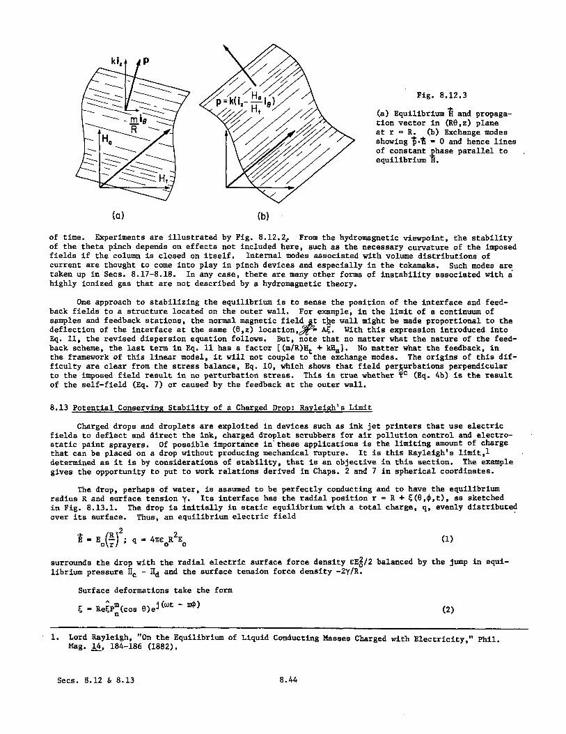
Fig. 8.12.3

(a) Equilibrium i and propaga-tion vector in (RO,z) planeat r = R. (b) Exchange modesshowing $1i = 0 and hence linesof constant phase parallel toequilibrium H.

(a) (b)

of time. Experiments are illustrated by Fig. 8.12.2, From the hydromagnetic viewpoint, the stabilityof the theta pinch depends on effects not included here, such as the necessary curvature of the imposedfields if the column is closed on itself. Internal modes associated with volume distributions ofcurrent are thought to come into play in pinch devices and especially in the tokamaks. Such modes aretaken up in Secs. 8.17-8.18. In any case, there are many other forms of instability associated with ahighly ionized gas that are not described by a hydromagnetic theory.

One approach to stabilizing the equilibrium is to sense the position of the interface and feed-back fields to a structure located on the outer wall. For example, in the limit of a continuum ofsamples and feedback stations, the normal magnetic field t the wall might be made proportional to thedeflection of the interface at the same (e,z) location,V= AE. With this expression introduced intoEq. 11, the revised dispersion equation follows. But, note that no matter what the nature of the feed-back scheme, the last term in Eq. 11 has a factor [(m/R)Ht + kHal. No matter what the feedback, inthe framework of this linear model, it will not couple to the exchange modes. The origins of this dif-ficulty are clear from the stress balance, Eq. 10, which shows that field perturbations perpendicularto the imposed field result in no perturbation stress. This is true whether Tc (Eq. 4b) is the resultof the self-field (Eq. 7) or caused by the feedback at the outer wall.

8.13 Potential Conserving Stability of a Charged Drop: Rayleigh's Limit

Charged drops and droplets are exploited in devices such as ink jet printers that use electricfields to deflect and direct the ink, charged droplet scrubbers for air pollution control and electro-static paint sprayers. Of possible importance in these applications is the limiting amount of chargethat can be placed on a drop without producing mechanical rupture. It is this Rayleigh's limit,1

determined as it is by considerations of stability, that is an objective in this section. The examplegives the opportunity to put to work relations derived in Chaps. 2 and 7 in spherical coordinates.

The drop, perhaps of water, is assumed to be perfectly conducting and to have the equilibriumradius R and surface tension y. Its interface has the radial position r = R + E(8,0,t), as sketchedin Fig. 8.13.1. The drop is initially in static equilibrium with a total charge, q, evenly distributed

over its surface. Thus, an equilibrium electric field

E = E R; q = 4e R2E (1)

surrounds the drop with the radial electric surface force density EE2/2 balanced by the jump in equi-librium pressure Hc - ld and the surface tension force density -2y/R.

Surface deformations take the form

S= Re P (cos 6)eJ( - (2)

1. Lord Rayleigh, "On the Equilibrium of Liquid Conducting Masses Charged with Electricity," Phil.Mag. 14, 184-186 (1882).

Secs. 8.12 & 8.13 8.44

with normal vector and surface tension force den-sity summarized in Table 7.6.2.

Bulk Relations: With the perturbation inelectric field from that given by Eq. 1 repre-sented by a = -VO, the Laplacian nature of thefields surrounding the drop is represented bythe flux-potential transfer relation, Eq. (d) ofTable 2.16.3:

ec . (n+l)Rcr R

Similarly, the inviscid fluid within is repre-sented by the pressure-velocity relation,Eq. (i) of Table 7.9.1 in the limit 8 + 0,

Ad Ad R Adpd= j PF (O,R)vd = -jwp - vn: r n r

Boundary Conditions: The electrical boundarycondition at the drop interface requires that therebe no tangential electric field: n x I = 0. Thiscondition prevails if frequencies of interest arelow compared to the reciprocal charge relaxationtime of the drop. With the objective of evaluatingthe electric field at the perturbed position of theinterface, note that to linear terms Eq. 1 is evalu-ated at the interface as

S r=R+E

,- - - -

Fig. 8.13.1. Spherically symmetric equilibriumfor a drop having total charge q uni-formly distributed over its surface.

SE(1 - 2-)0o

Then, Eq. M of Table 7.6. is used to represent 'nand, to linear terms in 5 and hence e, the boundarycondition is written in terms of amplitudes evaluated at the unperturbed interfaces I-c (4

c^C = EO

Continuity requires that (Eq. 7.5.5 to linear terms)

yr =

Stress equilibrium for the interface, in general given by Eq. 7.7.3, is written with the perturba-

tion pressure outside the drop ignored because the density there is negligible compared to that of the

drop. Thus,

c - d - (pdH- - (p')c d

28 E1 2 o E ec + (T) r= Trjn + (Ts) = •-•E 0

+ Ee + (T)rj j sr 2 oo R oor r

The equilibrium terms balance out, so that with the complex amplitude of (Ts)r given by Eq. (M)of Table 7.6.2,

2C E2

-d ooR + E E 8c -- (n - 1)(n + 2)•

oor R2R

Dispersion Relation and Rayleigh's Limit: All terms in the stress balance, Eq. 9, are written interms of 5 by using Eq. 6 in Eq. 3 for $, and Eq. 7 in Eq. 4 for Ad. The factor multiplying A in theresulting homogeneous equation is the dispersion equation:

w pR2 = (n - l)n[- (n + 2) - e E• ]R oo

The surface deflections are pictured with the help of Tabld 2.16.3.

n = 0 mode. From Eq. 10, the two n = 1 modes are neutrally stable.either along or transverse to the z axis.

(10)

Conservation of mass excludes theThese are pure translations,

The first modes to become unstable as Eo is increased are the three n = 2 modes. This is seenby solving Eq. 10 for the Eo that makes the term in brackets vanish and recognizing that this is first

Sec. 8.138.45

true for the lowest allowed value of n, n = 2. Thus, because Eo = q/4?r% 2 , it follows that Rayleigh'slimit on the total drop charge consistent with a stable equilibrium is

q =8 (11)

From this result, slowly increasing the net charge causes the drop to burst by fissioning into two drops.In most situations, the instability is dominated by the most rapidly growing of a spectrum of unstablemodes with growth rates predicted by Eq. 10.

8.14 Charge Conserving Dynamics of Stratified Aerosols

If charge can relax instantaneously on the time scale of interest, an interface and even bulkmaterial of fixed identity can preserve its potential. Examples are given in Secs. 8.13 and 8.7. Inthe opposite extreme are motions that conserve the charge density in the neighborhood of material offixed identity. A physical example is the transport of submicron charged particles entrained in air.By virtue of applied or self-fields, these particles migrate according to the laws investigated inSec. 5.6. But there, the gas flow was assumed to be known. What if the force transmitted to the gasby the charged particles results in a gas motion that dominates the migration of the particles relativeto the gas? In fact, because of .their extremely low mobilities, fine particles of high density canresult in a sufficient force on the gas that the resulting fluid motions dominate over migration indetermining the transport of the particles. Typically, what is observed is transport of particles byturbulent mixing with its origins in the electrohydrodynamic instability examplified in this section.

If fluid convection dominates over migration (or relaxation) in the transport of charged particlesby an incompressible fluid, then the charge density is related to the fluid flow by

Dpf-- =0 (1)Dt

In Sec. 7.2, this same statement was made for the mass density of an incompressible fluid. The generallaws and relations subsequently developed in Secs. 7.8 and 7.9 bear on the motions of a mass densitystratified fluid in a gravitational field much as does this section on motions of a charged fluid in anelectric field. The discussion of gravity-capillary dynamics, Sec. 8.9, exemplifies the dynamics offluids stratified in mass density, and is an example of how piecewise continuous models represent sys-

tems that are inhomogeneous in mass density.

At least as discussed here, where effects of self-gravitation are ignored, 9 in the gravitational

force density is constant, whereas the electric field t in the electric force density is a function of

the distribution of the field source, in this case pf. But, in regions where the charge density is con-

stant, say pf = q, the force density transmitted to the fluid by the charged particles neverthelesstakes the form of the gradient of a pressure:

SpfEp = -pfV =-V; E q4 (2)

Note that this statement prevails only where pf is constant. It cannot be used to deduce a stress

tensor at a boundary where pf is discontinuous, for example.

That the force density in regions of uniform charge density is the gradient of a pressure effec-

tively uncouples the bulk fluid mechanics from the electromagnetics. The inviscid equations of motion

are as given in Sec. 7.8, with C as defined by Eq. 2. Thus, in the bulk, vorticity is conserved by a

surface of fixed identity, and Eqs. 7.8.10 and 7.8.11 determine the velocity and pressure of motions

initiated from a state of zero vorticity.1

Planar Layer: Suppose that a planar layer is embedded in a system in such a way that the equi-

librium fields generated by the space charge are x-directed, as shown in Fig. 8.14.1. Because the

following comments are general, for the moment consider the layer to have an equilibrium uniform

translation in the z direction with velocity U. With G defined by Eq. 2, the pressure follows from

Bernoulli's equation, .Eq. 7.9.4, as

p (x) =- 2pU - q + -pgx

p' = p(-- + U a-),' - q'

1. The piecewise uniform approximation used here is developed in various geometries by M. Zahn,

"Space Charge Coupled Interfacial Waves," Phys. Fluids 17, 343 (1974).

Secs. 8.13 & 8.14 8.46

where primes indicate the time varying perturbation. A hybridperturbation pressure is now defined,

7r' p' + q0' (4) 1\

It follows from Eq. 3 that w is related to the velocity potential .. " " .

S= jp( - kzU)O (5)

Thus, 7r now has the same relationship to the velocity potential .----'.. -. .. . . .---as did $ in Sec. 7.9 (Eq. 7.9.6). Here, as in Sec. 7.9, 0satisfies Laplace's equation. Thus, the pressure-velocityrelations of Table 7.9.1 apply with . Fig. 8.14.1. Uniformly charged planar

Fig. 8.14.1. Uniformly charged planar

On the electrical side, Poisson's equation must be layer of charge conserving fluid.

satisfied at every point in the bulks However, because pf isconstant, the equilibrium field equilibrates the charge density in Poisson's equation and perturbationsin the potential must satisfy Laplace's equation. Thus, fields take the form

A j (t-k y-k z) dE d#0 (6)o= 0 (x) + Re e -~ =dx ; Eo dx

0

where the flux-potential transfer relations of Table 2.16.1 apply to the perturbation, Q.

Boundary Conditions: The electromechanical coupling occurs in the regions of singularity betweenlayers of uniformly charged fluid. Interfacial boundary conditions representing the mechanical equa-tions come from continuity, which requires that

Ax = j 4 (7)

and stress equilibrium. The charge density has a step discontinuity at the interface, but there is nosurface charge. Further, there is no discontinuity in the permittivity at the interface. Thus, thesurface force density, represented by the first term on the right side of Eq. 7.9.6, is zero. For

layers of charged aerosol, it is appropriate to ignore the surface tension, so the boundary condition is

simply

a9p =0 (8)

In view of Eq. 3, this condition is represented by its x-component evaluated to linear terms on the inter-

face at x (say) to give

qEo - pgj Z + JRI - Jq4) = 0 (9)

where Eo is now the equilibrium electrical field evaluated at the unperturbed interface.

The potential must be continuous at the perturbed interface. Because there is no surface charge

and no discontinuity in permittivity, it is also true that a Eo1 = 0, so this condition requires that

A =0 (10)

Because there is no surface charge even on the perturbed interface, a further boundary condition reflect-

ing Poisson's equations is that t~iE E = 0, so this condition requires that

Eqj Z + Co0 ex = 0 , (11)

where Eq. 6 is used to replace deoEo/dx by (q). The four boundary conditions, Eqs. 7, 9, 10 and 11, areevaluated at the unperturbed position of the interface.

Stability of Two Charge Layers: As a specific example, consider the motions of the layers shownin Fig. 8.14.2. In the bulk, the mechanics in each layer is represented by Eqs. (c) of Table 7.9.1with ý + ft:

Rc -coth(ka) s1nh(a) csinh(ka) x

=k--- (12)

Id -1 coth(ka) dsinh(ka) x

Sec. 8.148.47

1 .Aesinh(kb) x

cfcoth(kb) v

(13)

Similarly, the fields follow from Eqs. (a) of Table. 2.16.1:

-coth ka)

=k-1

sinh(ka)

-coth(kb)

=k

-1sinh(kb)

sinh(ka) c)

coth(ka) dj

1 esinh(kb)'

coth(kb)JL J

(14)

,Re

Lf1

Fig. 8.14.2.uniformhave anbounded

Fluid layers of differentcharge and mass densitiesinterface, d-e, and areby rigid electrodes.

(15)

Boundary conditions at the top electrode are

v = 0x

4c =0

at the interface are Eqs. 5, 7, 8 and 9:

Ad _e = jAx x

[Eo(qaqb) - g(paPb)] + (de) (qada e 0

^d _ e = 0

(q - qb ) + E ( ed _ e ) = 0

and at the bottom electrodes are

^fv =0

v= 0

(16)

(17)

(18)

(19)

(20)

(21)

(22)

(23)

It is a simple matter to substitute Eqs. 16-18,20,22, and 23 into the bulk relations.the resulting Eqs. 14b and 15a into Eq. 21 then shows that

Ad Ae -(qa- qb)

Sk[coth(ka)+ coth(kb)]o

The force-equilibrium boundary condition, Eq. 19, is finally

to obtain the dispersion equation

Substitution of

(24)

evaluated using Eqs. 12b and 13a and Eq. 24

W2 (qa - qb)2

-. [acoth(ka) + pb coth(kb)] = g( b-Pa)+Eo(a-b) coth(a)+ coth(kbk akcoth(ka) + coth(kb)]o

(25)

Remember that Eo is the equilibrium electric field evaluated at the unperturbed position of the inter-face. The equilibrium fields imply that the voltage Vo is related to Eo and the charge densities by

Sec. 8.14

-coth (kb)

JWP b

k-1

s inh (kb)

1.

a q5 9*(d),E 4.- -77.-. 7,

:.b ." b'Pb(e).±.LVo

F ,

ex.d

^f

7

8.48

Vo qbb 2 - qaa 2E + (26)o b+" 2e (a+b)

The last "self-field" term in Eq. 25 is positive regardless of the relative charge densities, andhence tends to stabilize all wavelengths. However, for short waveA (ka >> 1 and kb >> 1) its contribu-tion is negligible compared to the gravitational and "imposed field" term. Thus, a necessary and suf-ficient condition for all wavelengths to be stable is that the first two terms on the right in Eq. 25be positive,

g(Pb - Pa) + Eo(qa qb) > 0 (27)

The static arguments used in Sec. 8.4 lead to a similar condition, Eq. 8.4.11, because instability isincipient at zero frequency.

If the inequality of Eq. 27 is not satisfied, Eq. 25 shows that the growth rate of instabilitiesincreases linearly with the wave number. Actually, there is a wavelength for maximum rate of growththat would be predicted if the model included effects of viscosity (which come into play at shortwavelengths) or recognized the finite structure of the discontinuity in charge density.

The model of a charge density that is frozen to the fluid is of course relevant only if theprocesses described take place on a time scale short compared to the migration time of the chargedparticles. To what physical situations might the model apply?

Suppose that the electromechanical waves are of interest and Vo is adjusted to make E0 = 0. Fora fluid of uniform mass density (Pa = Pb = p ), according to Eq. 25, short waves have the frequency

S a= (28)

(Note that this is a reciprocal electro-inertial time.) For particles having charge q, number density nand mobility b, the self-precipitation time due to migration is Te = co/nqb) (Eq. 5.6.6). The frozencharge model is valid if the electro-inertial frequency given by Eq. 28 is high compared to the recipro-cal of the self-precipitation time. That is, for Iqa-qb| = nq, it is valid if

WT = >>1 (29)e 2 b

The summary of typical mobilities given by Table 5.2.1 makes it clear that the model does not apply toions in a gas. However, it could apply to charged macroscopic particles in air2 and to ions inliquids.3,4 In fact, as a consequence of the electrohydrodynamic instability that prevails when Eq. 27is not satisfied, the electrically induced convection can be a dominant charge transport mechanism.

The effect of the instability on transport of an aerosol is demonstrated by the experiment shownin Fig. 8.14.3.5 Generated by dry ice immersed in water, the aerosol passes from left to right as alayer, bounded from below by an electrode and from above by clear air. Thus, the configuration isessentially that of Fig. 8.14.2 with the upper region uncharged. The aerosol is negatively chargedby ion impact at the left. From the picture center to the right, the layer is subjected to a verticallyapplied electric field. In Fig. 8.14.3a, the applied field is upward and hence the configuration isstable. Some migration is observed, but little convection. In Fig. 8.14.3b, the field is reversed.Electrohydrodynamic instability is a arent in its contribution to the transport of charge out of thegas stream. For this experiment, eo/p/2b > 10, so effects of convection are expected to be important.

2. R. S. Withers, J. R. Melcher and J. W. Richmann, "Charging, Migration and ElectrohydrodynamicTransport of Aerosols," J. Electrostatics 5, 225-239 (1978)

3. P. K. Watson, J. M. Schneider and H. R. Till, "Electrohydrodynamic Stability of Space-Charge-Limited Currents in Dielectric Liquids," Phys. Fluids 13, 1955 (1970).

4. E. J. Hopfinger and J. P. Gosse, "Charge Transport by Self-Generated Turbulence in InsulatingLiquids Submitted to Unipolar Injection," Phys. Fluids 14, 1671 (1971).

5. R. S. Colby, "Electrohydrodynamics of Charged Aerosol Flows," B.S. Thesis, Department of ElectricalEngineering and Computer Sciences, Massachusetts Institute of Technology, Cambridge, Mass., 1978.

Sec. 8.148.49

(a)

(b)

Fig. 8.14.3. Aerosol passed through ion-impact charging re.gion at left and into region of applied electric field from the center to the right. The aerosol is charged negativep'. (a) Staole configuration with applied field directed upward. (b) Unstable configuration with ap­plied field reversed.

8.15. The z Pinch with Instantaneous Magnetic Diffusion

The model exemplified in this section pertains to the MQS dynamics of electrical conduction in the opposite extreme of that considered in Sec. 8.12. There time scales of interest were short compared to the magnetic diffusion time, so that the magnetic flux linked by a surface of fixed identity was con­served. In the opposite extreme considered here, the diffusion of magnetic field on the time scales of interest is instantaneous. In the magnetic diffusion equation, Eq. 6.2.2, the induction and "speed­voltagen terms are now negligible. That is, the magnetic diffusion time Tm = ~at2 is short compared to times of interest and the magnetic Reynolds number R = ~atv is small (Eq. 6.3.9).m

In this limit of instantaneous magnetic diffusion, the effect of the material deformation on the + +

magnetic field comes from the heterogeneity of the conductor. The distribution of J and hence H is determined by the geometry of the conductors. This is best emphasized by dealing with the current density rather than the magnetic field. Because R «1, the effect of motion on the current density is ignorable. Thus

m

+ + J = aE (1)

It follows from the law of induction, Eq. b.2.3 with T IT « 1 and R «1, that m m

(2)

Sees. 8.14 & 8.15 8.50

In the MQS approximation, the current density is also solenoidal:

V*J= 0 (3)

This is insured by Ampere's law, which represents J in terms of a "vectorpotential" which happens to be the magnetic field intensity:

+ +J = Vx H (4)

In regions where a and P are uniform, it follows from Eqs. 2 and 4 andthe solenoidal nature of A that

V = 0 (5)

which is of course the limit Tm/T << 1 and Rm << 1 of Eq. 6.2.6.

Liquid Metal z Pinch: The column of liquid metal shown inFig. 8.15.1 initially has a uniform circular cross section andcarries a longitudinal current density, Jo, that is uniform over thiscross section,

= Jo z (6)

Thus, by contrast with the perfectly conducting pinch of Sec. 8.12where the current is on the surface, the equilibrium magnetic fieldhas completely diffused into the conductor. It assumes the lineardistribution consistent with Amp're's law and Eq. 6: Fig. 8.15.1. Column of liquid

metal has static equi-or librium with 5 = 0 and

{ r2 r < R uniform axial currentH = (7) density.

oR 2

2r r > R

Static equilibrium prevails because the radial pressure distribution, p(r), just balances the associatedradial magnetic force density and surface tension surface force density. With p defined as zero in theair surrounding the column,

p = - 1 J 2 (r2 - R2) + (8)4 Odo R

An experiment demonstrating the dynamics to be described (Ref. 2, Appendix C) makes use of aliquid jet of mercury. In the model now developed, the longitudinal streaming of the jet is ignored.Instabilities exhibiting a temporal growth here can be displayed as a spatial growth as a result of thestreaming. Such effects of streaming are taken up in Chap. 11.

Bulk Relations: With the vector potential A 4 H and B - J, the situation is formally the same asdescribed by Table 2.18.1. Axisymmetric perturbations from this static equilibrium now considered canbe described in terms of one component of the magnetic field, fl= 1(r,z,t)t. Here, A= A/r and interms of A(r,z,t), the perturbation current density is

1 DA - 1 DA -+J= +l i (9)r -5 r + rr ar

The axisymmetric solutions of Eq. 5 in cylindrical coordinates are discussed in Sec. 2.19. Solu-tions are of the form of Eq. 2.19.10 with 8 O0:

^ A rJ1 (Jkr)A = H , (10)

That is, the perturbation current density in the bulk is uncoupled fgom the mechanics and determined bythe geometry of the interface, which will determine the coefficient Hf.

By contrasc, the mechanics is bulk coupled to the field distribution. The strategy in Sec. 8.14was to represent the electromechanical bulk coupling in terms of a force density that was the gradient

Sec. 8.158.51

of a pressure. Essentially, this attributes the coupling to interfaces. Here, part of the force densityis rotational, so that matters are not so simple. It follows from Eqs. 6 and 7 that

2+ + ~o Jdr o 0JorF =J x H =-i + J'x ie + oiz x H' (11)

o 29 r 2 i o

Thus, in view of Eq. 9, the force equation for the fluid becomes

p L- + V = r-o i ;at r r

Jo A7T - p' + 2

where the part of the force density that is the gradient of a pressure is lumped with the perturbationp'. Effects of gravity and viscosity are not included in Eq. 12. What is on the right in the force ofEq. 12 is the rotational part of the magnetic force density.

Because of this "one-way" coupling of the field to the fluid, it is necessaryamounts to the transfer relations,for the fluid. The r and z components of Eq. 12,tinuity condition V.v = 0, give three relations for the mechanical perturbations:

jwp +r dr r

jWp• z - jk* = 0

1 d (r r) - jk- = 0r dr r z

to rederive whatas well as the con-

(13)

(14)

(15)

Elimination of Vz between Eqs. 14 and 15 gives an expression that can be solved for 9,Z

wp = d (re)2 d (16)

Substitution of this expression into Eq. 13 gives

d2,dvr

dr2

1 dOr r 2^ jk2J2oo A+ k v =

r dr 2 r wp rr

(17)

In the absence of-the bulk coupling, these last two expressions could be used to derive the pressure-velocity transfer relations of Table 7.9.1. Added to the homogeneous solutions of Eq. 17 (that comprisethese transfer relations) is now a particular solution satisfying the equation with Eq. 10 substitutedon the right. Substitution and recognition that Jo(jkr) satisfies Eq. 2.16.19 with m = 0 shows that aparticular solution is

(18)j(jkR)rJ (jkr)2wpJ1(jkR) o

where Eq. 2.16.26c has been used. Of the two homogeneous solutions, the one that is not singular at theorigin is Jl(jkr). The linear combination of particular and homogeneous solutions that makes r (R)=vris

1dJl(jkr)v vr r Jl(jkR), PokHa RJo (jkR)J (jkr)

2wpJl(jkR) Ji kR - rJ (jkr2mpJ 1 (jkR) JjkR) o

(19)

Thus, in view of Eqs. 12-and 16, the amplitude of the perturbation pressure is

= J (j k r )

k Jl(jkR) ro2jkJ(jkR)

2jkJ1(QkR)

jkR J (jkR) -2(r 1 ( jI o J (j k r ) - 2J (jkr) + 2jkrJ1(jkrLJ1(j kR) 0 0a

Boundary Conditions: The effect of the boundary condition on the distribution of current density,and hence magnetic field, is represented by the condition that at the interface, *.J= 0. To linearterms, with A written in terms of C(z,t) (Eq. (e) of Table 7.6.2),

r + jk = 0 (21)

Sec. 8.15

(12)

(20)

r ur r

8.52

The radial current density, Jr, is substituted into this expression using Eqs. 9 and 10 to show that

This condition represents the effect of the mechanics (geometry) on the field.

The return effect of the field on the fluid is taken into account in writing stress equilibrium forthe interface. Note that there is no singularity in the magnetic force density at the interface. Thatis, there is no surface current and no discontinuity in magnetizability of the material. Hence, the mag-netic surface force density, i Te J n , makes no contribution to the stress equilibrium, Eq. 7.7.6.Because the fluid surrounding thecoldmn is of considerably lesser density than the column, the perturba-tion pressure, ^c, is ignored. Thus, the jump in total pressure evaluated at the perturbed position ofthe interface is balanced by the surface tension surface force density, Eq. (f) of Table 7.6.2:

-{-p [(R + ) 2 - R2 d =[-+ + 5] (23)4 0 RR R 2 z

By design, the equilibrium part of this balance cancels out. In terms of complex amplitudes, the perturba-tion part is

1 2' d (24)o/ Rý - d = [1 - (kR)2 (24)

^dEvaluated using Eqs. 20, 22 and the continuity condition vr = jw~, this expression becomes the dispersionequation

2 pR3 kRI1(kR) j02OR3 2(kR) 21o(kR) 22pR kR=1 12 21-2(kR) 1 + [(kR) - 1] (25)Y I(kR) 1 2 kRI(kR)

Rayleigh-Plateau Instability: The normalized frequency given by Eq. 25 is shown as a function ofwave number by Fig. 8.15.2 with the magnetic pressure o (daR)2/2 normalized to the surface tension pres-sure y/R as a parameter. Negatives of the quantities shown are also solutions. Note that even in theabsence of an axial current, perturbations kR < 1 (wavelengths longer than 27TR) are unstable. Any per-turbation results in major radii of curvature that differ in sign. For a region that is necking off,the curvature associated with the axial dependence tends to restore the equilibrium whereas that causedby the circular cross section of the column tends to further neck off the column. For perturbationshaving wavelength X > 2wR, the latter wins and the equilibrium is unstable. The wavelength for maximumrate of growth, given by kR = 0.7, can be used to give a rough prediction of the size of drops formedfrom a liquid jet. According to the linear theory, a drop having radius ro would have a volume equal tothat of one wavelength of the jet, 7rR2 = 4/3(rr3).

Fig. 8.15.2

Normalized frequencyS=W/pR3/y as a

function of wave num-ber. --- Wi, -- r.The parameter is

J~o2R 3 /2y.

KIN

Sec. 8.15

t'S

8.53

z-Pinch Instability: The general nature of the pinch instability is qualitatively similar to thatfound with the flux conserving pinch of Sec. 8.12. Because the current through the column must be con-served, both the current density and the magnetic field intensity in the fluid adjacent to the inter-face go up wherever the column tends to neck off. The result is an inward magnetic force density thattends to further encourage the necking off. Unless wavelengths are sufficiently short to be stabilizedby surface tension, they are unstable. According to the model, it is only the inertia of the columnthat limits the rate of growth of the instability.

Finally, is the instantaneous magnetic diffusion model appropriate for the description of a mercurycolumn having a radius of 1 cm or less? From Eq. 25 and Fig. 8.15.2 the frequency can be taken as ofthe order of /y/pR3. For the approximation to be justified, the product of this frequency (or growthrate) and the magnetic diffusion time (based here on the column radius) must be small:

22m

m P(26)

-3Typically, this number is less than 10- 3

The major electromechanical effect that would be experimentally observed but not accounted for bythis model is magnetic damping.

8.16 Dynamic Shear Stress Surface Coupling

It is a straightforward process to include the effects of viscosity in the piecewise homogeneousmodels developed in Secs. 8.9-8.15. The fluid mechanics is represented by the viscous diffusiontransfer relations of Sec. 7.19 rather than the inviscid pressure-velocity relations of Sec. 7.11. Withthe viscosity come additional boundary conditions. At an interface, not only is the normal velocitycontinuous, but so also is the tangential velocity (Eq. 7.7.3). Also, the shearing stresses acting atan interface, Eq. 7.7.6, are not automatically balanced. In Secs. 8.9-8.15, the interfacial stressbalance is for interfaces free of shearing surface force densities. Thus, any of these examples havestress balance equations in directions tangential to the equilibrium interface that are identicallysatisfied.

In this section, the example treated not only illustrates how viscosity is taken into account in

piecewise homogeneous systems, but also involves an electric shearing surface force density. Hence, the

viscous shear stresses are necessary for the formulation of a self-consistent model.

A highly insulating liquid, such as hexane, has a free surface which is bounded from above by agas, as shown in Fig. 8.16.1. Perhaps by means of a very small radioactive source, some ion pairs

are provided in the bulk of the liquid. By means of a potential applied between the planar electrodes,half of this charge is swept to the interface where it forms a monolayer of surface charge that shields

the electric field from the liquid; thus, Go = EEo. Subjected to a tangential electric field, common

interfacial ions migrate relative to the liquid at a rate that is negligible compared to that due to

convection. A good model pictures the charge as frozen to the liquid interface. What are the modesof motion characterizing the adjustment of the inter-face to a perturbation field?

Because the fluids to either side of the inter-face have uniform permittivities and no free chargedensity, the electromechanical coupling is confinedto the interface. In the following, it is assumedthat the depth of the liquid and the distance to the

upper electrode from the interface are large comparedto typical perturbation wavelengths on the interface.

Static Equilibrium: With *the interface flat and Fig.v = 0, the electric field is

= Eoix x; x > 0=E 0o

0 "; x < 0

and the pressure balances the gravitational force density inequilibrate the surface force density coE2/2:

00

1E. +

------. - --9-

8.16.1. Cross section of liquid-air inter-face supporting surface charge density

oo . Charges are modeled as frozen tothe liquid.

(1)

the liquid with a jump at the interface to

x> 0-xx= 1pgP

1 2x + - E E - ;

2 oo

Sec. 8.15 & 8.16

x< 0

8.54

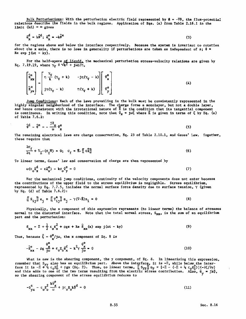
Bulk Perturbations: With the perturbation electric field represented by 4 = -VO, the flux-potentialrelations describe the fields in the bulk regions. Application of Eqs. (a) from Table 2.16.1 in thelimit (kA) - O gives

ed = kOd; e = e-ke (3)x x

for the regions above and below the interface respectively. Because the system is invariant to rotationabout the x axis, there is no loss in generality if perturbations are taken as independent of z; ' =Re exp j(wt - ky).

For the half-space of liguid. the mechanical perturbation stress-velocity relations are given byEq. 7.19.19, where yV E kZ + jwp/n,

A YV ^e

ie Ae'e '(Yv +k) vxSe jn( v - k) n(y + k) vY

Jump Conditions: Each of the laws prevailing in the bulk must be consistently represented in thehighly singular neighborhood of the interface. The charge forms a monolayer, but not a double layer,and hence consistent with the irrotational nature of E is thg condition that its tangential componentis continuous. In writing this condition, note that x = jmC where ' is given in terms of E by Eq. (a)of Table 7.6.2:

Ad Ae jEo e'd - =--- v (5)W x

The remaining electrical laws are charge conservation, Eq. 23 of Table 2.10.1, and Gauss' law. Together,these require that

a•- (f) = 0; af= . (6)

To linear terms, Gauss' law and conservation of charge are then represented by

-d Ae) - k ° e = (7)

For the mechanical jump conditions, continuity of the velocity components does not enter becausethe contributions of the upper fluid to the stress equilibrium is negligible. Stress equilibrium,represented by Eq. 7.7.5, includes the normal surface force density due to surface tension, y (givenby Eq. (d) of Table 7.6.2):

Sij n + Te nj - y(V*.)ni = 0 (8)

Physically, the x component of this expression represents (to linear terms) the balance of stressesnormal to the distorted interface. Note that the total normal stress, Sxx , is the .sumof an equilibriumpart and the perturbation:

S = E2+ EE + pgx + Re SS (x) exp j(Jt - ky) (9)xx 2 0o xx

Thus, because E = Ox/jw, the x component of Eq. 8 is

^e ^e

x ,d 2 x-S - pg + EoEoe - k2y -= 0 (10)xx j oox

What is new is the shearing component, the y component, of Eq. 8. In linearizing this expression,remember that S also has an equilibrium part. Above the interface, it is -TI,while below the inter-face it is -TI+ £oE0 2 + pgx (Eq. 2). Thus, to linear terms, I Syy ny [-TI - (-TI + ½ £oE 2) (-'a/y)an -hi-. oAAa -p ne nAf the +wa terms resultin from the elecri,. str•ss conntributio-n Abl. = 1

so the shearing component of the stress equilibrium reduces to Y

Se- E2 x + jEoE kd = 0 (11)yx oo W 00

Sec. 8.168.55

Dispersion Equation: By using Eqs. 3, the components (e ,ex) can be eliminated from the electricjump conditions, Eqs. 5 and 7, and these solved for ýd

-jE Eo +e vesd= o x o y (12)

SX= (12)W(Eo + E)

This expresses the effect of the mechanics on the fields.

The self-consistent electromechanics is now represented by the two stress conditions, Eqs. 10 and11, written in terms of the velocity amplitudes ( ). The strs amplitudes are elimited in favorof these variables using Eqs. 4, while eis written in terms of 4 by using Eq. 3a, and $ in turneliminated using Eq. 12. Thus, the two expressions are

2jEkE

o

WU + )E:w8+

0

o

EW(1 +

0-

jn (y V - k) j-(V + k) +L(l + -)(1 + 7-- )

- 1 0- 0-

ev

l1

l~e

0

0

(13)

Physical insights are more easily obtained by adding j times Eq. 13b to Eq. 13a, and writing both equa-tions (each multiplied by w) in terms of the variables exand (-_x + jz). Use is made of the defini-tions ao = EEn and y; E k2 + jwp/n:

+ 4akw - j(pg + k2y) + je kE2 [-2rikW]

kE E2[2jnkw] jn (YV + k)w + -

1+ 6-F_

0

ex

-e _e-vx+jvySy

0

0

(14)

The dispersion equation is obtained by setting either the determinant of the coefficients from Eq. 13

or from Eq. 14 equal to zero. But, written in the second form, it is clear that as the viscosity

approaches zero, two modes can be distinguished. These have limiting dispersion equations given by

setting the diagonal terms to zero. The frequencies resulting from the upper left and lower right

terms, respectively, are then

(=2nk 2 ± w aJ k (pg + k2y - ke E2 2nk2 2 (15)W =J + ) ;0 o+ k (-1 )

.r. 12/3U c + (16)

The modes can be distinguished in this way only if the frequencies given by Eqs. 15 and 16 are dis-

parate. In general, the higher order dispersion equation must be solved.

^e ^eWhen Eq. 15 is satisfied, Eq. 14 shows that v jv , and similarly, if Eq. 16 holds, then the

vertical motions are dominated by the horizontal ones, Ox 0. Thus, the dispersion equation (Eq. 15)

is identified with gravity-capillary like waves coupled to an electric field in much the same way as

discussed in the latter part of Sec. 8.10.

The main effect of viscosity on the gravity-capillary modes is damping, represented by the imagi-

nary term in Eq. 15. Perhaps a surprising feature of these modes in this low-viscosity limit is that

the electric field has the same destabilizing effect as if the interface were perfectly conducting. For

example, the condition for incipient instability is the same as given by Eq. 8.10.21, even though that

result was derived for an equipotential interface. In this low-viscosity limit, the surface charge on

the insulating interface is convected sufficiently rapidly to maintain the interfacial potential con-

stant.

The electromechanical oscillations or shear waves, represented by Eq. 16, involve interfacial

dilatations. If an interfacial region is horizontally compressed, self-fields give rise to horizontal

Sec. 8.16

v-

~' v v

8.56

electric repulsion forces, much as if there were an elastic film on the interface. Because this elec-trical "film" is coupled to the inertia of the liquid below through the viscous shear stress, an initialhorizontal dilatation of the interface results in oscillations. The oscillations are highly dampedbecause the electrical "spring" is coupled to the "mass" only through the viscous "damper." The fre-quency Wc typifies how rapidly nonuniformities in a charged interface can adjust, so that the interfaceis free of electrical shear stress. The motion stops when the interface is an equipotential.

SMOOTHLY INHOMOGENEOUS SYSTEMS AND THEIR INTERNAL MODES

8.17 Frozen Mass and Charge Density Transfer Relations

A static EQS equilibrium with mass density Po(x) and charge density qo(x) continuously varying withvertical position is shown in Fig. 8.17.1. The equilibrium vertical gravitational and electrical forcedensities are balanced by a vertical gradient in pressure. It is the objective in this section todescribe small amplitude perturbations from this equilibrium.

The mass density and charge density are conserved by a fluid element of fixed identity,

DpD 0; = 0DDt Dt

The fluid has uniform permittivity e and it is inviscid.

'''; ..· :::.:.;: · : .

q(x) E (x) x) .

.0.......q---/100)

Fig. 8.17.1

Planar layer of fluid with verticalinhomogeneities in mass and chargedensities.

7It will be recognized that this system is a generalization of the piecewise homogeneous systems

considered in Secs. 8.9 and 8.14. In principle, any distribution of po(x) and go(x) could be approxi-

mated by "stair-steps" representing stratified layers, with uniform densities, as illustrated in

Fig. 8.17.2. The transfer relations for the homogeneous layers might then be used to represent the

approximated system. With each interface goes a pair of modes, so

that the piecewise homogeneous approximation represents the dynam-

ics in terms of twice as many modes as interfaces. In the limitof a smooth distribution, an infinite number of modes are broughtinto play. Hence, it should come as no surprise that associatedwith the smoothly distributed inhomogeneities are an infinitenumber of "internal" modes. The objective in this and the nextsections is to explore an approach that is an alternative to thepiecewise homogeneous models.

In manipulations that follow, remember that Po, qo and Eoare functions of x. By Gauss' law, DEO = qo/e, Where d( )/dx ED( ). Thus, in terms of complex amplitudes and E Qx/jw, Eqs. 1relate perturbations in mass and charge density to the deformation

Fig. 8.17.2. Stair-step approxi-mation to smooth inhomo-geneity in po(x) or q0 (x).

S-(Dp o ) ;

The additional statements represent force balance, mass conservation, that the electric field is irrota-tionalAand Gauss' law. These are unraveled so as to obtain four first-order differential equations in

The z-component of the force equation can be solved for Oz to obtain

a ~kz wp0

where the perturbation electric field A = -VO and # E p + qo0. Thus, the continuity equation, V.- = 0,

Secs. 8.16 & 8.17

~-~3C(

......-----------

A = -(q

8.57

requires that

kgk 2

W z 2po

In view of Eqs. 2, the x component of the force equation requires that

Dl= (w2 po - EoDq 0 + gDpo)t + (Dq 0) (5)

where x is replaced by -DO and p represented in terms of ft.That 1 is irrotational is also explicitlystated,

DO =- I (6)

Finally, Gauss' law, together with Eq. 2b, gives

D(EAx ) =x + jkee z =-Dqog - k 2EO (7)

Given the amplitudes ( •,p,B,e) at the lower extremity of the layer (say x = 0), these last fourequations can be numerically integrated and the amplitudes evaluated at the upper extremity. Thus therelations

*ce

xe

= Bij I

XIx

(8)

are obtained. For example, to compute the Bij's, the equations are integrated with ( ,p ,' ,e•) =(1,0,0,0). Then, (B11 ,B1 2 ,B1 3 ,B14) are the computed values of (Xfa, O,Eea), respectively. x

Transfer relations in the form

~ftc

ActCex

CexX

= Icij IC$a

(9)

follow by manipulating Eqs. 8. With the 4x4 matrix Cij divided into four 2x2 submatrices, transductionbetween electrical and mechanical surface variables is represented by the upper right and lower leftsubmatrices. In the absence of coupling (say, with qo = 0), these entries should vanish. In this samelimit, the upper left submatrix relates the pressure to the velocity amplitudes and these relations playthe role of those derived in Sec. 7.9. Of course, here the layer has a nonuniform equilibrium mass den-sity. Also in this limit, the lower right matrix relates the electric perturbation flux to the poten-tials. Because the layer has uniform electrical properties, these should become the same as the 2x2entries in relations given by Eq. (a) of Table 2.16.1.

An alternative way of expressing Eqs. 4-7 results from combining the first three of these ex-pressions to obtain

A2 N kDqoD(poD0) + k2 - Po2 2 0 (10)

where N/ EoDqo - gDpo and the last two to obtain

2 2 Dqo&(D - k )= E (11)

This pair of second-order expressions can be used to determine (E,O) and the remaining pair of vari-ables (9,eFx) then evaluated using Eqs. 4 and 6. The first of these expressions represents force equi-librium between the inertial force density and the gravitational and electric force densities. The"imposed-field" electric force density is on the right. The second expression is Poisson's equation.

Sec. 8.17 8.58

On the right is the perturbation space charge generated by the convection of the nonuniform equilibriumcharge density.

The driven response, spatial modes and temporal modes are illustrated in Sec. 8.18.

Weak-Gradient Imposed Field Model: Two approximations make it possible to obtain analytical ex-pressions for the Cij. First, the mass and charge densities are taken as being linear functions of x.Hence,

Po = m + (Dpm)x; qo = qe + (Dqe)x (12)

where pm,Dp ,qe and Dq, are constants and neither po nor qo departs greatly from a mean value. Then,Eqs. 10 and 11 are approximated by

D2+ 2 A 22-=; 2 - ( - 1)k2 (13)

0 m m W2 2 Dqe

(D ) (14)

Secondly, the field E0 is regarded as largely imposed by means of external sources. Then, notonly is E0 approximated by a constant, but the coupling between fluid and field, represented by theterms on the right in Eqs. 13 and 14, is relatively weak. This breaks the electromechanical feedbackloop.

First, to determine the mechanical response, the effect of the motion on the charge distributionis ignored in determining the potential distribution. With the term on the right in Eq. 14 set tozero,

S• sinh(kx) _ ~ sinh k(x-6) (15)sinh(kA) sinh(kA)

This potential is used as a "drive" to evaluate the right-hand side of Eq. 13. By inspection, thesolution satisfying the boundary conditions that C is Co and V at the respective planes is

a 2 ^"a F 2 1k2qaDe sin(yx) + k Dq• sin y(x-A)

[ 2Pm(k2+y )J sin(A) + + 2 2 sin(yA)

(16)k2Dqe a sinh(kx) _ $B sinh k(x - tA)

S2 +(k22 sinh(kA) sinh(kA)

To find the approximate electrical response, the procedure is reversed. Given that ( is ( and 5at the respective planes, solution of Eq. 13 with the term on the right ignored gives

=a sin(yx) _ - sin y(x - ) (17)sin(yA) sin(yA)

In turn, the solution of Eq. 14 is

a Dqe sinh(kx) Dqe 1 sin k(x - A)+ +s- L-+kkjS y + k2 sinh(kA) 2+ k2+ sin(yA)

Dqe a sin(yx) _ sin y(x - (18)

2 + k2 sin(yA) sin(yA) (18)

where coefficients are determined by inspection so that the boundary conditions on 0 are satisfied atthe respective planes. The covariables (*,Eg ) follow from Eqs. 4 and 6 and are evaluated at therespective boundaries to give the transfer refations, Eqs. 9, with

Sec. 8.178.59

C1 = -C22 2 cot(yA)

m2Pm

C = -C =21 12 2

k sin(yA)

Dq eC1 3 = -C24 = -C31 42 2 2 [k coth(kA) - y cot(yA)]k +y

Dq [ yk ] (19)

14 23 32 41 k2 2 sin(yA) sinh(kA)

C33 = -C = -sk coth(kA)'

EkC = - = k34 43 sinh(kA)

Although the weak coupling approximation is sufficient to give the mechanical response to an elec-trical drive or the electrical response to a mechanical drive, the electrical-to-electrical response,represented by C3 3 , C3 4 , C4 3 and C4 4 is devoid of any of the electromechanics. Electromechanicaleffects on the transfer between electrical signals depend on there being a "two-way" interaction.

Reciprocity and Energy Conservation: That some coefficients, Cj, in the transfer matrix haveequal magnitudes suggests that basic relations exist between off-diagonal coefficients even with arbi-trary gradients and fields. The frozen charge model is free of dissipation and allows for energy

storage in electrical, kinetic and gravitational forms. With variables as defined in Eq. 9, this re-quires that the submatrix representing the hybrid pressure responses to electrical excitations is the

negative of that representing the electrical flux responses to mechanical deformations. It also re-quires that mutual electrical and mutual mechanical coefficients are respectively negatives. The proofis a generalization of that developed in Sec. 2.17 for a region storing only electric energy.

Incremental changes in the total electrical, kinetic and gravitational energy stored by a system

having volume V enclosed by a surface S are respectively

w = p dV - 6Dnda (20)e S

6sk = IfVf.6tdV - fsp6-*.da + fvpg.6ýdV (21)

6w = f (---)6pdV (22)

The electrical contribution is familiar from Sec. 2.13 (Eq. 2.13.4). The kinetic statement exploits

Newton's law and the incompressibility condition to state that all work done by the electrical, mechan-

ical and gravitational subsystems goes into the creation of kinetic energy (Eq. 7.17.3). The gravita-

tional energy storage is familiar as a specialized analogue of the electric one. The scale is small

enough that gravitational self-fields are neglected and g is constant. Thus, by contrast with the

potential 4 for the electrical system, the gravitational potential is "imposed" and is simply -g.r.

Charge migration is negligible, so the charge carried by fluid of fixed identity is conserved.

Because V.6r = 0, it follows (from Eq. 3.7.5 with ci - q) that

6q = -Vq.-6 (23)

Similarly, the mass density of fluid of fixed identity is conserved,

6p = -Vp.~ (24)

These expressions are now used in writing the sum of Eqs. 20-22 as

6 (we + wk + wg) = - f da - p6*da - J(Vq + qVb), 6dV

S S (25)

-S [pV(-.) + (-e..)Vp].6dVJV

Sec. 8.17 8.60

where use has also been made of the relations E = -VD and = V(J-2). The volume integrals are con-

verted to surface integrals by first using a vector identity to contract the integrands [OV+YV4=•=V(TYb)]

and then exploiting the fact that V.6 = 0 to make the integrands take the form of perfect divergences

(VT.- = V.A - A.lY). From Gauss' theorem, it follows that

6 (we +wk +wg) = - 6 da - [p + cq + (-j.?)p]6 .Ada (26)

S S

The desired reciprocity relations are between perturbation quantities, now designated by primes todistinguish them from the zero-subscripted equilibrium variables. Thus, incremental changes 6M*$ and6V*A on S lead to changes in the total energy given by Eq. 26 expressed up to quadratic terms in theperturbations as

6 (we +wk + wg) = - 0 6 0 da - (0 6•' + V'60 + V'D')*.da

(27)

- + [po o + (- p o]6t'da - S[p o + + (- )p']6'da

The surface S is now made one enclosing a section of the planar layer shown in Fig. 8.17.1 thathas the wavelengths 2r/ky and 2T/kz in the y and z-directions, respectively. Because ýo is x-directed,the first term makes contributions only on the a and B surfaces. Perturbations are assumed to take thecomplex-amplitude form E = Reý exp(-jky - jkzz), where ky and kz are real. The spatial periodicity in

the y and z dir&ctions insures that contributions to the surface integrations from the second and third

terms only come from the a and 8 surfaces. Moreover, because the integrands of these terms are linearin the perturbation quantities, they "average out" and make no contribution. The quadratic perturbationterms from the last intergral, which are also periodic and hence make contributions only on tfe a and 8surfaces, can be represented using the space-average theorem, Eq. 2.15.14:

6(w + wk + w ) = -(O6DO - - 1 Re(c 6(D)- 6(D ) ]e k g o xo o xo 2 x x

- -a- - Re q 1 B*] (28)

_ _ -, _~B,," 1 Re(--.)[ p(* - -6 (- Re[q 6(i )* q- • B( *] - Re(- r)[

6( *

With the understanding that the incremental variations are made with the equilibrium potentials o0held fixed on the transverse boundaries, the first terms on the right become perfect differentials,

0o0Dxo + 6 (4oDxo), so these equilibrium terms are moved to the left side of the equation.

In the remaining terms, it is now assumed that all complex amplitudes are real. It is entirely

possible to ~rogeed w thout making this assumption by treating the real and imaginary parts of the

variables (ý P, j,,P ) as independent. However, there is little to be learned from this generalizationbecause it is obvious from Eqs. 4-7 (which, provided w2 is real, have real coefficients) that the co-efficients Cii are real. Hence, given that the amplitudes ( O,,VJcOi,) are real, the amplitudes of the

conjugate variables are clearly real.

In the forth and sixth terms of Eq. 28, Eqs. 2 are used to substitute

Sj65 = -0 Dq 6 z 6( o•Dqo 2 ) (29)

(-_=-)i 6 -_(-_ )Dpo - 16(-_.1))Dp Z2 ] (30)

respectively. The second equalities are based on recognition that if variations in the Z's and Dx's

result in variations of Dqo or DPo, the latter can be neglected, because the terms in which they appear

are already quadratic in the perturbations. With the substitution of Eqs. 29 and 30, the fourth and

sixth terms also become perfect differentials and are therefgre moved to the left side of Eq. 28.Finally, in the second term on the right the transformation 0

6Dx = 6(Dx) - Dx6f is made and the perfectdifferential moved to the left-hand side. Thus, the energy statement becomes

Sec. 8.178.61

6w' I=-l (-a ) + I.(B6ai_ B061B) (31)

where

e k g 2 x X 4 0 0 0w' ~we k g a ge ( - - q ( )2

1- (- [Dp a2 - Dp B()2] + -a )4 o xo o xo

and

Now, with the assumption that w' is a state function w'I(X,c,',aa8), the incremental change 6w'can also be written as

6w' = w. 6 + -w'6 + w. ia + w' 60 (32)

Because the variables (Z ,Z ,a,8)are independent, it follows from Eqs. 31 and 32 that correspondingcoefficients must be equal:

T = -2--- ; IT = 2 a(33)

b = 2 ; = -2Ž (34)x ail x 810

The reciprocity relations follow by taking cross-derivatives of these relations. For example, in viewof Eqs. 33a and 34b together with Eq. 9,

3ia aDb- C14 = C41 (35)

Thus, if Cij is broken into four 2x2 matrices K, L, M and N such that

C =[K L]M N(36)

where K and N are each antisymmetric and L is the negative of M.

The next section exemplifies the implications of the transfer relations, both found by numericalintegration and approximated by the weak-gradient imposed-field model.

8.18 Internal Waves and Instabilities

The frozen charge and mass density transfer relations derived in Sec. 8.17 are now applied to thestudy of space-charge gravity waves excited in the sinusoidal steady state from transverse boundaries.Also discussed are the temporal and spatial modes. Instability conditions are exemplified and a generalproof given that the principle of exchange of stabilities is satisfied. With the objective of bothgaining physical insight for this type of dynamics and for ways in which it can be represented, twomodels are developed and compared. First, the weak-gradient imposed-field approximation of Sec. 8.17is used to obtain an analytical representation of the response. Then, as a recourse that is applicablefor an arbitrary distribution of charge and mass density, numerical integration is used to determinethe response. Because one of these representations depends on numerical procedures, it is convenientto normalize variables "at the outset.

Configuration: The stratified layer shown in Fig. 8.18.1 is bounded from above by fixed excita-

tion electrodes upon which a spatially and temporally periodic potential is imposed. From below, itis bounded by a conducting rigid electrode, essentially constrained in potential to the constant equi-librium value Vo .

Normalization: To be specific about the distributions in charge and mass density, they are takenas linear and written in terms of the constants defined in Fig. 8.18.1:

Secs. 8.17 & 8.18 8.62

,,=Redej(t-kz)

d... ..i g..:: E"x).Fig. 8.18.1

Cross section of system inwhich internal space-chargegravity waves are excited.

Dpm+ -PMPm

In terms of these quantities, variables are normalized such that

x = xd

k = k/d

2 2 VolDqelpdm

ii- lo

= ;IDqell 0vldS= (dIV

d = •x = dlDqIdx x -x e

For other equilibrium distributions, the same normalization

IDqel defined as mean values.could be used with the quantities Pm and

From the one-dimensional form of Gauss' law and the equilibrium potential boundary conditions, theequilibrium distribution of electric field is written in terms of the normalized variables as

Vo Vo e 1 1 Dqe 2 10o d o 2j7 - 3TV0

where SE .qeld2/ElVo represents the influence of the space charge on the imposed field.

Driven Response: Boundary conditions reflect electrode constraints on the normal motion of the

fluid and on the potential:

a ,b,a ,b = [0,0,V,0]

Given the electrical excitation at the upper boundary, what is the mechanical and electricalresponse of the fluid, and in particular, what perturbation pressure and normal electric field wouldbe expected on instruments embedded in the lower electrode? These follow from Eq. 8.17.9 as

^bfb dx^ C23; ^ 43

V V

In the weak-gradient imposed-field approximation, it is possible to evaluate the C 's by usingEqs. 8.17.19. Thus normalized, Eq. 3 becomes

C-2 3 -1 k

dDq k2 + y2 sin y sinh k

C4 3 1Vo_ -1 kC43- Dqe d2 sinh k

Sec. 8.18

II

Dq,I

9m gqSVO

Pm

qo(x)o q

so -e- 1

Dq1 + e x;

qe -

^bC

S 23V

^bd

9

-4

PoP o= P 1p 1

8.63

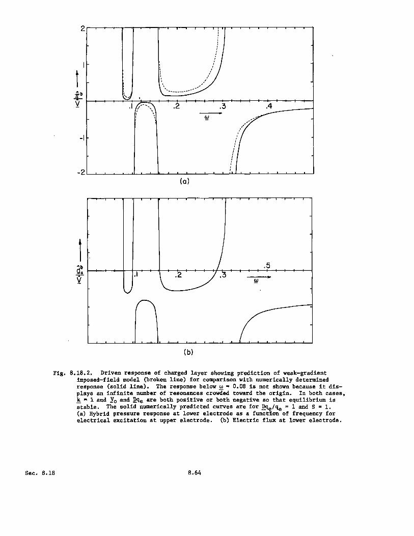
14

Fig. 8.18.2. Driven response of charged layer showing prediction of weak-gradientimposed-field model (broken line) for comparison with numerically determinedresponse (solid line). The response below w = 0.08 is not shown because it dis-plays an infinite number of resonances crowded toward the origin. In both cases,k = 1 and Yo and kqe are both positive or both negative so that equilibrium isstable. The solid numerically predicted curves are for Dqe/qe = 1 and S = 1.(a) Hybrid pressure response at lower electrode as a function of frequency forelectrical excitation at upper electrode. (b) Electric flux at lower electrode.

Sec. 8.18

I

^b:

Tvd

8.64

where

YEk +-] -d1-1 (8)

The upper sign applies if Vo and Dqe are both positive or both negative. The lower sign is to beused if Vo and Dqe have opposite signs.

The weak-gradient imposed-field driven responses are illustrated as a function of frequency inFig. 8.18.2. Because of approximations inherent to this model, the electrical-to-electrical responseis no more than that of the layer without the charged fluid. This result will be refined to includethe electromechanical effects shortly. The resonances in the hybred pressure response that dominatethe picture reflect the electromechanical coupling. In this loss-free system, they serve notice thatthe natural frequencies of the stable temporal modes are real and that there are an infinite numberof spatial modes having real wave numbers. The conditions for the resonances follow from Eq. 6:

sin y = 0 = y = nrr,n = 1,2,..* (9)

Thus, the resonance frequencies are found by evaluating y in Eq. 8 and solving for w,

V

2 k 2 /V Dq - gDPmW 2 ; N= Voe m (10)

k + (nr) IDqd Dqe

The associated distributions, E(x), in the neighborhood of a resonance follow from Eq. 8.17.17 asbeing sin(nrx). These are pictured by the broken curves of Fig. 8.18.3. Implicit to the discussionthus far is the presumption that N> a.

Ix

Fig. 8.18.3

Vertical displacement of fluid asa function of vertical position.Response is shown in the neighbor-hood of first and second resonances,and hence represents first and sec-ond temporal eigenmodes. Solidcurves are predicted numericallyusing parameters of Fig. 8.18.2,while broken curves are weak-gradient imposed-field approxi-mation.

Consider now the more general approach of numerically integrating Eqs. 8.17.4-7 to find thetransfer relations. Normalized, these equations are

k2DC = k2 (11)W P0

= (w2 DqoD = (p -N) +_ (12)o }EDq (2

Sec. 8.188.65

nD = -. dx (13)

Dqo 1 2Dd = - Dq - 1 (14)JxDqeI

5e

These expressions are applicable with arbitrary charge and mass distributions. For the specific lineardistributions, po is given by Eq. 2, Dqo = Dqe and

o Dqe Sre 1 1 2 11 Dqe gdDpmf + IDq Sl (x-2)+ (x -3) q o- (15)

The coefficients required to evaluate the responses, Eqs. 3, follow by converting the transferrelations of Eq. 8.17.8 to those of Eq. 8.17.9. The coefficients needed here are

C23 = -B14 /D; C43 = B12/D; D2 B12B34 B1 4B32 (16)

Coefficients in the transfer relations have been normalized so that Sij and Bij relate normalized veri-ables. The Bi 's are determined by numerical integration of Eqs. 11-1i following the procedure indicatedfollowing Eq. A.17.8. (Numerical integration of systems of first-order differential equations writtenin the form of Eqs. 11-14 is conveniently carried out using standard library subroutines. Used here wasthe IMSLIB Routine DVERK.)

For purposes of comparison, the numerically determined frequency responses are shown with thosepredicted by the weak-gradient imposed-field model in Fig. 8.18.2. For the numerical case shown,Dqe/qe = 1 and S = 1, so both the weak-gradient and the imposed-field approximations are somewhat in-valid. Note that the electrical-to-electrical response now displays the characteristic resonances ofthe internal waves. The numerically determined mechanical displacement and potential distributions withthe frequency in the neighborhood of the first and of the second resonances are shown in Fig. 8.18.3.

Spatial Modes: Still in the sinusoidal steady state, these modes satisfy homogeneous transverseboundary conditions and are needed to make the total solution obey longitudinal boundary conditions.(Spatial modes are introduced in Sec. 5.17.) For example, what is the response to a drive at somez plane with the duct walls free of excitations?

From the weak-gradient imposed-field driven response of Eq. 6, the dispersion equation isD(w,k) = sin Y = 0. This has roots that are the same as for the resonance conditions, Eq. 10. Here,however, interest is in complex k for a real driving frequency w,

nawk =+ nrw (17)

Under the assumption once again that N/V > 0, the dispersion equation is typified by Fig. 8.18.4. Notethat all modes have the same cut-off frequency . = 1. With ) < 1, all modes are propagating, whereaswith w > 1, all modes are evanescent.

The resonances below w = 1 in the driven frequency response, Fig. 8.18.2, result from a coinci-dence of the imposed wave number and the purely real wave number of the propagating spatial modes.

Temporal Modes: When t = 0, initial conditions are spatially periodic in the z direction, withwave number k. What modes are to be superimposed in representing the ensuing transient? (Temporalmodes are introduced in Sec. 5.15.)

A mode En(x) has the eigenfrequency jin E sn. Without being specific as to the charge and den-sity distributions, it can be deduced from Eqs. 8.17.10 and 8.17.11 together with the boundary con-ditions that these eigenfKequencies are either purely real or purely imaginary so sn is real. Equation8.17.10 is multiplied by En and integrated over the cross section. The first term is then integratedby parts to obtain

*^ d d ^* d2 N I/

* d Dqonpo nDn o poDnD ndx - k (p + -) n dx = -k 2 2 dx (18)

0 n ]n o o0o n o f o s 2n n

Similarly, the complex conjugate of Eq. 8.17.11 is multiplied by k2E0n and integrated over the crosssection. Again, the first term is integrated by parts to obtain

2 ADA* d 2.d •A 4. fd A * 2)d A*^

k nDo ] -k28 Dn(DO) dx - k o dx = k Dq 0 4 dx (19)n no n o n n o0 n no o

Sec. 8.18 8.66

fIW

O 2 4 6 8k-----

The point of these manipulations is to obtain positive definite integrands anq to make the right-handsides of these expressions negatives. Because of the boundary conditions on En and On, the termsevaluated on the boundaries vanish. Thus, the last two expressions give

d 22 d(Id PDn2 + pk 2In 2)dx = -p- 2 /fNjn 2 + Fc(IID• 2 + k2 2)]dx (20)n a 0

n2

This expression can be solved for the square of the eigenfrequency, Sn,

-k2[ d n 2 A+(D•* - k2" * ) ]dx

s2 o (21)Jd[po(IDnI + k nI)dx

2Terms on the right are real, and it thereforR follows that sn is real. Moreover, because terms in thedenominator are positive definite, as is k21n,12 in the numerator, it is clear that if /Nis everywherepositive, the eigenmodes are all stable:

N- EDq0 - gDp > 0 (22)

Similarly, if /Vis everywhere negative, the eigenmodes have an exponential dependence, half of themdecaying and half of them growing in time.

Using the weak inhomogeneity imposed-field approximations, the eigenfrequencies follow fromEq. 10 where this time k is a given real number. These are shown as a function of k in Fig. 8.18.5.According to this model, in the unstable configuration ( A/< 0) the n = 1 mode is the most rapidlygrowing.

It is worthwhile to make a comparative study of the discretely and smoothly stratified chargelayers. The condition of Eq. 22 plays a role relative to the smoothly inhomogeneous system that isplayed by Eq. 8.14.25 for the piecewise homogeneous system of Sec. 8.14.

Sec. 8.18

X

n=2

Fig. 8.18.4

Complex normalized frequency asfunction of real longitudinal

n=3 wave number for spatial modes inweak-gradient imposed-field ap-proximation. Wr - , wi ....All modes have common asymptoticfrequency at w = 1, above whichthey are evanescent.

8.67

±wn(N>0)

±s(N< 0)1

0 2 4. 6k -

Fig. 8.18.5

Weak-gradient imposed-field eigenfre-quencies of temporal modes as a func-tion of wave number. For N> 0, allmodes are stable and purely oscilla-tory. For N< 0, they are eitherexponentially growing or decayingwith time.

Sec. 8.18 8.68