1+1 National Libraryof Canada

Bibliothèque nationaledu Canada

Acquisitions and Direction des acquisitions etBibhographic services Branch des services bibliographiques

395 Wellington Street 395. rue WellingtonOttawa. anl.rio Ottawa (Onl'rio)K1AON4 K1AON4

NOTICE AVIS

The quality of this microform isheavlly dependent upon thequality of the original thesissubmitted for mlcrofilming.Every effort has been made toensure the highest quality ofreproduction possible.

If pll~es are missing, contact theuniversity which granted thedegree.

Some pages may have indistinctprlnt especlally if the originalpages were typed wlth a poortypewriter ribbon or If theuniversity sent us an Inferlorphotocopy.

Reproduction ln full or ln part ofthls mlcroform ls governed bythe Canadlan Copyright Act,R.S.C. 1970, c. C-30, andsubsequent amendments.

Canada

La qualité de cette microformedépend grandement de la qualitéde la thèse soumise aumicrofilmage. Nous avons toutfait pour assurer une qualitésupérieure de reproduction.

S'il manque des pages, veuillezcommuniquer avec l'universitéqui a conféré le grade.

La qualité d'impression decertaines pages peut laisser à .désirer, surtout si les pagesoriginales ont étédactylographiées à l'aide d'unruban usé ou si l'université nousa fait parvenir une photocopie dequalité Inférieure.

La reproduction, même partielle,de cette mlcroforme est soumiseà la Loi canadienne sur le droitd'auteur, SRC 1970, c. C-30, etses amendements subséquents..,.,

•

•

•

CONTRIBUTIONS TO THE KINEMATICSYNTHESIS OF PARALLEL

MANIPULATORS

Hamid Reza Mohammfldi Daniali

B.Sc. (Mashhad University), 1986

M.Sc. (Tehrc.n Unj·.'ersity), 1989

Department of Mechnical Engineering

McGill University

Montreal, Quebec, Canada

A thesis submitted to the Faculty of Graduate Studies and Research

in partial fulfillment of the requirements for the degree of

Doctor of Philosophy

March 1995

© Hamid Reza Mohammadi Daniali

.+. National Libraryo!canada

~uisilions andBibliographie Services Branch395 Welfinglon Street0t1awa. ontarioKIA llN4

Bibliothèque nationaledu Canada

Direction des acquisitions etdes services bibliographiques395. Ml WellinolonOttewa (Onterie)K1AllN4

THE AUTHOR HAS GRANTED ANIRREVOCABLE NON·EXCLUSIVELICENCE ALLOWING THE NATIONALLmRARY OF CANADA TOREPRODUCE. LOAN, DISTRIBUTE ORSELL COPIES OF HISIHER THESIS BYANY MEANS AND IN ANY FORM ORFORMAT, MAKING THIS THESISAVAILABLE TO INTERESTEDPERSONS.

THE AUTHOR RETAINS OWNERSHIPOF THE COPYRIGHT IN HISIHERTHESIS. NEITHER THE THESIS NORSUBSTANTIAL EXTRACTS FROM ITMAY BE PRINTED OR OTHERWISEREPRODUCED WITHOUT HISIHERPERMISSION.

ISBN 0-612-05759-3

Canadrl

L'AUTEUR A ACCORDE UNE LICENCEIRREVOCABLE ET NON EXCLUSIVEPERMETTANT A LA BmLIOTHEQUENATIONALE DU CANADA DEREPRODUIRE, PRETER, DISTRIBUEROU VENDRE DES COPIES DE SATHESE DE QUELQUE MANIERE ETSOUS QUELQUE FORME QUE CE SOITPOUR METTRE DES EXEMPLAIRES DECETTE THESE A LA DISPOSITION DESPERSONNE INTERESSEES.

L'AUTEUR CONSERVE LA PROPRIETEDU DROIT D'AUTEUR QUI PROTEGESA THESE. NI LA THESF,.NI DESEXTRAITS SUüSTANTIELS DE CELLE- •CI NE DOIVENT ETRE IMPRIMES OUAUTREMENT REPRODUITS SANS SONAUTORISATION.

•

•

•

..

•

•

•

Abstract

This thesis is devoted 1.0 the kinematic synthesis of parallel Illauipulat.ol's at. hu'ge,

special attention being given 1.0 three versions of a novel c1ass of Illanipulat.ol's,

named dOllblc-ll'ianglllal'. These are conceived in planaI', spherical and spat.ial double­

triangulaI' varieties.

The treatment uf planar and sphel'ical manipulatol's needs only plaual' aud sphel'­

ical trigonometry, a fact that inductively leads 1.0 the succcssfui treatlllent of spat.ial

varieties with methods of spatial trigonometry, whercin t.he relationships are cast. in

the form of dllal-nllmbcl' algebraic expressions. Using the forcgoing l.ools, t.he dil.'ect.

kinematics of the three types of doublc-triangular mauipulatol's is fOl'lllulat.ed and

resolved.

• Moreover, a general three-group classification, 1.0 deal with sinYllllLl'ilics encouu--tered in parallel manipulators, is proposed. The classification schellle relies on the

properties of .Jacobian matrices of parallel manipulators. 11. is shown l.hal. ail singu­

larities, within the workspaccs of the manipulators of interest, arc readily identified

if tbeir .Jacobian matrices arc formulated in an invariant form.

Finally, the optimal design of the manipulators is studied. These designs llIin­

imize the roundoff-error amplification clrects duc 1.0 the nUlllerical inversion of the

underlying Jacobian matrices. Such designs arc called isoll'Opic. Based on this

concept the multi-dimensional isotropic design continua of several manipulators arc

derived,

ii

•

•

•

Résumé

Cet.te thèse porte sur la synthèse cinématique des manipulateurs parallèles généraux,

et plus particulièrement, sur une nouvelle classe de manipulateurs, dite à double­

triangle. Ces manipulateurs se présentent en version planaire, sphérique et spatiale.

L'analyse de ces manipulateurs, en version planaire et sphérique, nécessite seule­

ment des relations trigonométriques planaires et sphériques, induisant ainsi l'utilisation

avec succès de relations trigonométriques spatiales pour la version spatiale de ces ma­

nipulateurs. Ces relations sont écrites sous forme d'expression algébrique à nombres

duals. Le problème géométrique direct des troiS versions de manipulateurs à double­

triangle est formulé et résolu avec cet outil mathématique.

De plus, une classification générale des manipulateurs parallèles en trois groupes

est proposée. Celle-ci repose sur les propriétés de la matrice Jacobienne des manip­

nlateurs. Elle montre que toutes les singularités, situées à J'intérieur de l'espace de

travail dn manipulateur étudié sont facilement identifiées si la matrice Jacobienne

('st écrite sous forme invariante.

l~inalement, la conception optimale des manipulateurs est étudiée, afin de min­

imiser les effets d'amplification des erreurs d'arrondissement lors de l'inversion de la

matrice Jacobienne. Les manipulateurs ainsi conçus sont appelés isotropes. En se

basant sur ce concept, l'auteur obtient le continuum multi-dimensionnel de plusieurs

manipulateurs isotropes.

Hi

•

•

•

Acknowledgements

Sincere gratitude is extended to my supervisor, Professor Paul .1. ZsomhOl'-l'l'llII'ray,

and my co-supervisor, Professor Jorge Angeles, for assistauce and guidaucc, aud

especially for suggestions which motivated, facilitated and enlmnced my rese,u·ch.

Thankfully, the Ministry of Culture and Higher Education of the Islamic Republic

of Iran made my work possible by granting me a generous scholarship. This was

augmented by additional support from NSERC.

Professors V. Hayward and E. Papadopoulos, provided me invaluable snggest.ions

in the early stages. Special thanks are due to Dr. Manfred Husty, Montanuniver­

sitat Leoben, for his enlightening insights into kinematic geometry and to Professor

O. Pfeiffer for guiding my design of practical planaI' and spherical double-triangulaI'

manipulators. Ali my colleagues and friends at Centre for Intelligent Machines (CIM)

shared with me their friendships and helped to make my studies at McGill a pleasant

experience. Particularly, 1 would like to thank John Oarcovich, for assistance with

computer animation, and Luc Baron for many enriehing discussions throughout. t.he

course of my research and for his French translat.ing of t.he abst.ract.. 'l'han ks arc also

due to CIM for offering state-of-UIC-art computer facilities and a pleasant research

environment.

The understanding, patience and support of my wife Masoumeh was unswerving.

1 am profoundly grateful for her great sacrifice on my behalf. The steadfast sup­

,port and encouragement of my family gave me the confidence and det.ermination to

'preserve.

iv

•

•

•

Claim of Originality

The author c1aims the originality of ideas and results presented here, the main con­

t.rihutions heing listed below:

• Introduction of three versions of a novel c1ass of parallel manipulators, namely,

planar, spherical and spatial douhle-triangular manipulatorsj

• solutions of the associatec! direct kinematic problemsj

• derivation of the Jacohian matrices for these and other classes of p~.rallel ma­

nipulators, hased on an invariant representationj

• classification of singularities in parallel manipulators into three groups, and

identification of ail three groups within the workspaces of the manipulatorsj

• derivatioll of multi-dimensioual continua of isotropie designs for sorne parallel

manipulatorsj

• expression of the screw matrix and its invariant paramet.~rs in invariant form.

'l'he material presented in this thesis has been partially reported in (Mohammadi

Daniali, Zsombor-Murray and Angeles, 1993a, 1993b, 1994a, 1994b, 1994c, 19!14d,

I!J95a, 1995b, 1995c. 1995d and Mohammadi Daniali and Zsombor-Murray, 1994).

v.: .

•

•

•

Dedicated to:

the memol'Y of my fatlwl". . ,

lllY lllotlwl';

IllY wHe and son.

•Contents

•

•

•

2.2.5 Thc Product of Two Liues

2.2.6 Dual Scrcw lvlatriccs

2.3 Spatial Trigouometry . .

2.3.1 Spatial Triangle . . .

2.3.2 PlanaI' Trianglc . . .

2.3.3 Spherical Triangle ..

2.3.4 Trigonomctric ldcntitics

3 Parallel Manipulators3.1 Introduction................

3.2 PlanaI' Manipulators .

3.2.1 3-DOF Manipulators of Class A .~.2.2 3-DOF Manipulators of Class B .

3.3 Spherical Manipulators .

3.3.1 Spherical 3-DOF, 3-RRR Mallipulator

3.3.2 Spherical 3-DOF, DT Manipulator

3.4 Spatial DT Manipulators . . . . . . . . . . . .

3.4.1 Spatial 6-DOI~, DT Manipulator ...

3.4.2 Othcr Versions of Spatial DT Mallipulators .

4 Direct Kinematics

4.1 Introduction .

4.2 PlanaI' Manipuiators .

4.2.1 PlanaI' 3-DOF, 3-RRR Manipulator .

4.2.2 PlanaI' 3-DOF, DT Manipulator .

4.3 Sphcrical Manipulators .

4.3.1 Spherical 3-DOF, ~:RRR Malliplilator

4.3.2 Spherical 3-DOF, DT Manipulator

4.4 Spatial DT Manipulators .

4.4.1 6-DOF Maniplilator .

4.4.2 Other Versions of Spatial DT Maniplilators .

5 Singularity Analysis

5.1 Introduction .

5.2 Jacobian Matrices. . . . . . . . . . . .

5.2.1 PlanaI' Maniplilators of Class A

viii

.)"_1

:12

38

'17

50

50

50

50

51

5li

5li

57fi4

fi4

71

75

75757li

•

•

ii.2.2 PlanaI' Manipulators of Class Bii.2.:l Spherical 3-RRR Manipulator .

5.2.1 Spherical DT Manipulator ...

.5.2..5 Spatial 6-DOF, DT Manipulator .

ii.3 Classification of Singularities .

05.3.1 PlanaI' Manipulators of Class A05.:3.2 PlanaI' Manipulators of Class B05.:3.:3 Spherical 3-RRR Manipulator ..

5.:3.1 Spherical DT Manipulator ....

5.:3.5 Spatial 6-DOF, DT Manipulator .

6 Isotropic Designs6.1 Introduction .

6.2 Isotropil Designs . . . . . . . . . . . .

6.2.1 PlanaI' Manipulators of Class A6.2.2 PlanaI' Manipulators of Class B6.2.:3 Spherical 3-RRR Manipulator .

6.2.1 Sphel"Ïcal DT Manipulator . . .

6.2.5 Spatial 6-DOF, DT Manipulator .

i8808182

85

8i929i

100102

107lOilOi109113

IIi

119

120

•

7 Concluding Remarks 125i.l Conclusions . . . . . . . . . . . 125

i.2 Consideration for Future Work . . 12i

References 129

Appendices 141

A Bezout's Method 141

B Coefficients of Equation (4.19b) 143

C Coefficients of Equation (4.38) 145

D Coefficients of Equation (4.41) 147

E Mechanical Designs of Planar and Spherical DT Manipulators 151

ix

•List of Figures

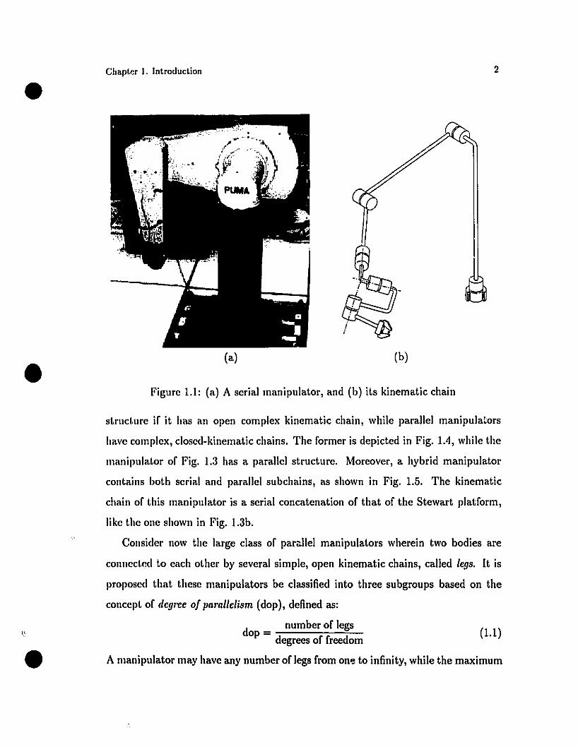
1.1 (a) A seriallllanipulator, and (b) its kincl1latic chain 2

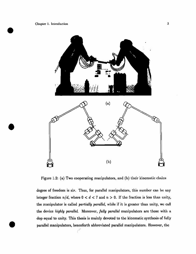
1.2 (a) Two cooperating Illanipulators, and (b) thcir kincl1la\,ic dmins :1

1.3 (a) Stewart platforlll, and (b) its kincl1latic chain '1

1.4 (a) A four-fingered hand (The Utah-MIT hal1(l), and (b) its kincl1lat.ie

chain. . . . . . . . . . . . . . . . . . . . fi

1.5 Hybrid manipulator; Logabex LX4 robot 5

•2.1

2.2

2.3

2.4

2.5

2.6?~~.I

2.8

2.9

Dual plane .

Dual angle between two skew Hnes

Plücker coordinates of a line

Vectors a, band s .

Layouts of Hnes A, 8 and S . . . .Screw motion of Hne A, about Hnc SSpatial triangle .

PlanaI' tl'Îangle .

Spherical triangle

171!)

1!)

22

2li

2!J

•

3.1 The graph of a general 3-dof, 3L parallcl Illaniplilator

3.2 The manipulator of c1ass A .3.3 PlanaI' 3-dof, 3-RRR parallel manipulator

3.4 The manipulator of c1ass 8. . .3.5 PlanaI' 3-dof, DT Illanipulator .

3.6 The spherical 3-dof, 3-RRR Illanipulator

3.7 The spherical 3-dof, DT manipulator .

3.8 The graph of a general 6-dof, DT array

3.9 Spatial DT manipulator .

3.10 Tlle graph of a general 3-dof, DT al'ray

x

45

4li

Mi

48

48

• 4.1 Geometrie model of the planaI' 3-dof, DT manipulator

4.2 Triangles Q and n .4.:1 Triangles Q, Q', 'P and n .4.4 Spherical triangles Q and n ..4.5 Spherical triangles Q, Q' and 'P4.6 Geometrie modcl of spatial DT manipulators

51

.52

56

.58

6.5

66

•

•

5.1 The ith leg of spherical DT manipulator . . . 82

.5.2 Example of the second type of singularity for the manipulators of class

A in which the three vectors Vi intersect at a point . . . . . . . . .. 88

.5.3 I~xamples of the first type of singularity for the planaI' 3-RRR manip­

ulator with (a) one leg fully extended, and (h) one leg fully folded .. 90

.5.4 Examples of the second type of singularity for the planaI' 3-RRR ma­

nipulator in which (a) the three vectors ri are parallel, and (h) the

three vectors ri intersect at a point . . . . . . . . . . . . . . . . . .. 91

.5 ..5 Examples of the third type of singularity for the planaI' 3-RRR ma­

nipulator in which (a) the three vectors ri are parallel, and (h) the

three vectors ri intersect at a point . . . . . . . . . . . . . . . . . .. 92

5.6 Example of the second type of singularity for the manipulators of class

B in which the three vectors ti intersect at a point 93

5.7 Example of the first type of singularity for the planaI' DT manipulator 9.5

5.8 Example of the second type of singularity for the planaI' DT manipulator 96

.5.9 Example of the third type of singularity for the planaI' DT manipulator 97

5.10 The first type of singularity of the spherical 3-RRR manipulator with

one leg fully extended. . . . . . . . . . . . . . . . . . . . . . . . . .. 98

5.11 The first type of singularity of the spherical 3-RRR manipulator with

one [eg folded . . . . . . . . . . . . . . . . . . . . . . . . . . . . .. 99

5.12 The second type of singularity of the spherical 3-RRR manipulator 100

.5.13 The third type of singularity of the spherical 3-RRR manipulator 101

.5.14 Spherical DT manipulator at the first type of singularity .. 102

5.1.5 Spherical DT manipulator at the second type of singularity . 103

.5.16 Spherical DT manipulator at the third type of singularity . . 104

5.17 Spatial 6-dof, DT manipu!ator at the first type of singularity 10.5

5.18 Spatial 6-dof, DT ,manipulator at the second type of singularity 106

.5.19 Spatial 6-dof, DT manipulator at the third type of singularity 106

xi

•

•

•

6.1 An isotropie design of a planar 3-RRR lllaniplIlator ..

6.2 An isotropie design of a planar DT maniplliator ....

6.3 An isotropie design of a spherieal 3-RRR Illaniplliator

6,4 An isotropie design of a spherieal DT manipulator

6.5 An isotropie design of a spatial 6-dof, DT Illaniplliator

E.l A typieal design of planar DT maniplIlators .

E.2 A typieal design of spherieal DT maniplliators

xii

Il:l

116

118

120

12'1

152

155

•List of Tables

1.1 General comparison of seriai and paral1el manipulators 6

•

•

2.1 Dual <Iuantities and their properties 28

4.1 The sixteen solutions of Example 4.3.2.1 64

4.2 The six solutions of Example 4.4.J.l . 71

4.:1 The 26 solutions of Example 4.4.2.1 . . . 73

5.1 Ai, Bi, Ci and Ej for different legs of the manipulators of class A 78

xiii

•

•

•

Chapter 1

Introduction

1.1 General Background

A manipulator, according to IFToMM l 's Commission A Standards for Terminology

(1991), is a device for gripping and the contml/ell movement of objcct,~, Examples

of manipulators appear in Figs. 1.1a-l.4a and 1.5. For the purpose of this thesis,

we regard the manipuiator as a kinematic chain of rigid links coupied by kincllllltic

pairs. A kinematic pair is, in turn, the coupling of two links so as to constrain their

relative motion. Kinematic chains arc classified as simple or complex, open or closed.

If the chain contains at least one link coupled to only one other link, the chain is

called open, as depicted in Fig. 1.1 bi otherwise it is closcd, Ils depiet,ed in Fig. 1.2b,

Moreover, a simple kinematic chain is one with links coupied to at most two other

links, while a complex kinematic chain is one with at least one Iink connected 1.0

threc or more links. Both Figs. LIb and 1.2b show simple kinematic chains, while a

complex kinematic chain is depicted in Fig. 1.3b.

Manipulators are classified here into four categories, namely, seriai, tl'ec-typc,

paraI/el and hybrid. The term seriai manipulator denotes an open, simple kinematic

chain structure, as shown in Fig. 1.1. A manipulator is said to have a trl.'C·type

llnternational Federation for the Theory of Machines and Mcchanisms

•

•

Chapter 1. Introduction

(a) (b)

2

(1.1)t'

•

Figure 1.1: (a) A seriai manipulator, and (b) its kinematic chain

struc\.ure if it has an open complex kinematic chain, while parallel manipulators

have complex, c1osed-kinematic chains. The former is depicted in Fig. lA, while the

nmniplliator of Fig. 1.3 has a parallel structure. Moreover, a hybrid manipulatol'

contains both seriai and parallel subchains, as shown in Fig. 1.5. The kinematic

chain of this maniplliator is a seriai concatenation of that of the Stewart platform,

like the one shown in Fig. 1.3b.

Consider now the large c1ass of parallel manipulators wherein two bodies are

conllectcd to each other by several simple, open kinematic chains, called legs. It is

pl'Oposed that these manipulators be c1assified into three subgroups based on the

concept of dcg/oce of parallelism (dop), defined as:

dnumber of legs

op-- degrees of freedom

A maniplliator may have any nllmber of legs from OM to infinity, while the maximum

•

•

Chapter 1. Introduction :1

(b) -

•

Figure 1.2: (a) Two cooperating manipulators, and (b) their kinematic chai liS

degree of freedom is six. Thus, for parallel manipulators, this number cali he allY

integer fraction nid, where 0 < d < 7 and n > O. If the fraction is Icss than unity,

the manipulator is called pal·tially pal'allel, while if it is greater than unity, wc cali

the device higilly parallel. Moreover, Jully parallel manipulators are thosc with a

dop equal to unity. This thesis is mainly devoted to the kinematic synthcsis of fully

parallel manipulators, henceforth abbreviated parallel manipulators. Howevcr, the

•Chaplcr 1. Inlroduclion

(a) (b)

4

•

•

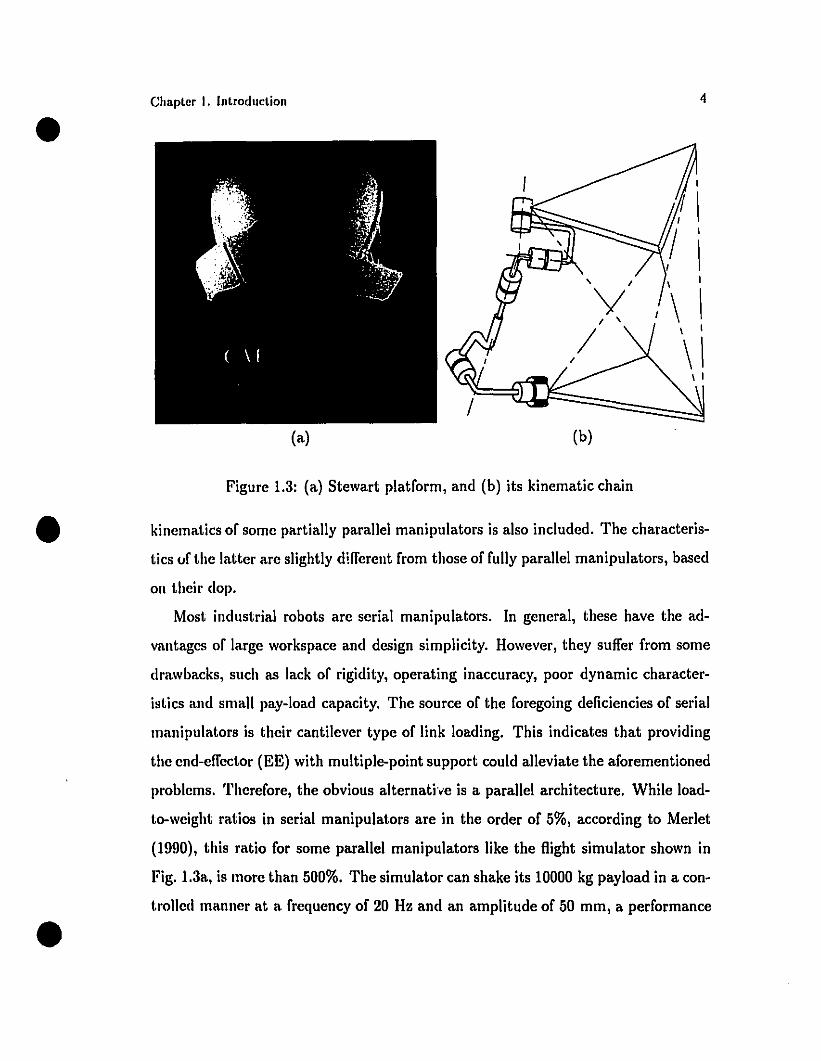
Figure 1.3: (a) Stewart platform, and (b) its kinematic chain

kinematics of sorne partially parallel manipulators is also included. The characteris­

tics of the latter arc slightly dilferent from those of fully parallel manipulators, based

on their dop.

Most industrial robots are seriaI manipulators. In general, these have the ad­

vantages of large workspace and design simplicity. However, they suifer from sorne

drawbacks, such as lack of rigidity, operating inaccuracy, poor dynamic character­

istics and small pay-Ioad capacity. The source of the foregoing deficiencies of seriai

manipulators is their cantilever type of link loading. This indicates that providing

the end-elfector (EE) with multiple-point support could alleviate the aforementioned

problems. Therefore, the obvious alternative is a parallel architecture. While load­

to-weight ratios in seriai manipulators are in the order of 5%, according to Merlet

(1990), this ratio for sorne parallel manipulators like the f1ight simulator shown in

Fig. 1.3a, is more than 500%. The simulator can shake its 10000 kg payload in a con­

trolled manner at a frequency of 20 Hz and an amplitude of 50 mm, a performance

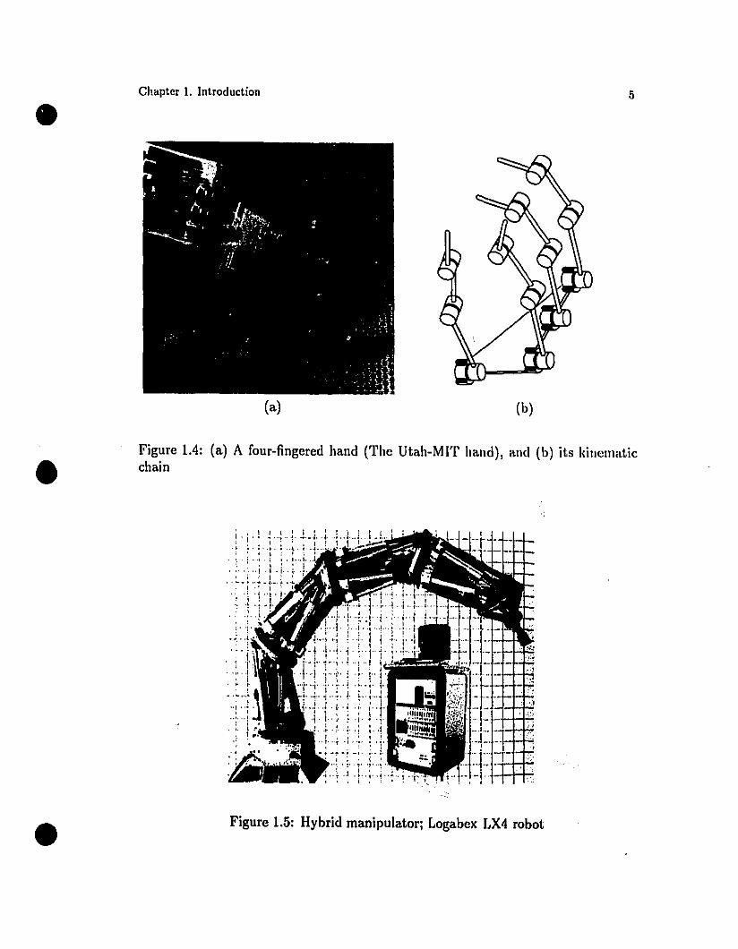
Figure 1.4: (a) A four-fingered hand (The Utah-MIT hand), and (h) its kinenllLticchain

•

•

Chapter 1. Introduction

(a) (h)

5

•

,!.;. 1....

i , 1..,. ;. ,...,., .... - ~ .. ". -1..­'" .1 :1 ..:,'!; ·1

1 : •'" "'" .L.

; ~ :.:. ':'

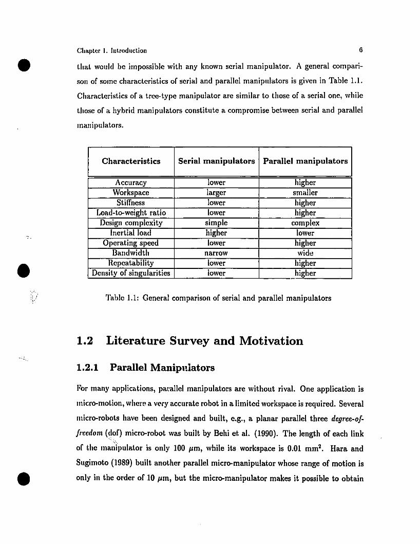
Figure 1.5: Hybrid manipulatorj Logabex LX4 robot

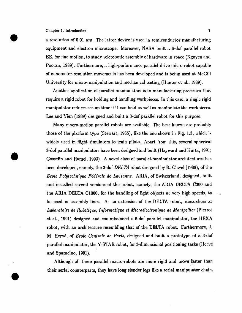
that wOllld be impossible with any known seriaI manipulator. A general cornpari­

son of sorne characteristics of seriai and parallel maniplliators is given in Table 1.1.

Characteristics of a trec-type manipulator arc similar to those of a seriaI one, while

those of a hybrid manipulators constitute a compromise between seriai and parallel

man ipulators.

•

•

Chapter 1. Introduction

Characteristics SeriaI manipulators Parallel manipulators

Accnracy lower higherWorkspace larger smallerStilfness lower higher

Load-to-weight ratio lower higherDesign complexity simple complex

Inertial load higher lowerOperating speed lower higher

Bandwidth narrow wideRepeatability lower higher

Density of singularities lower higher-

6

•

Table 1.1: General comparison of seriaI and parallel manipulators

1.2 Literature Survey and Motivation

1.2.1 Parallel Manipnlators

For many applications, pat'allel manipulators are without rival. One application is

micro-motion, wher~ a very accurate robot in a limited workspace is required. Several

micro-robots have been designed and built, e.g., a planaI' parallel three degree-of­

frecdom (dof) micro-robot was built by Behi et al. (1990). The length of each link

of the ma.;ipulator is only 100 Ilm, while its workspace is 0.01 mm2 • Hara and

SlIgimoto (1989) bllilt another parallel micro-manipulator whose range of motion is

only in the order of 10 Ilm, but the micro-manipulator makes it possible to obtain

a resolution of 0.01 /lm. The latter device is used in semiconductor manufacturing

equipment and electron microscope. Moreover, NASA built a 6-dof parallcl robot

EE, for fine motion, to study ",elerobotic assembly of hardware in space (Nguyen and

Pooran, 1989). Furthermore, a high-performance parallcl drive micro-robot capable

of nanometer-resolution movements has been developed and is being used at McGiIl

University for micro-manipulation and mechanical testing (Bunter et al., HJ8!J).

Another application of parallel m:mipulators is in manufacturing processes tlmt

require a rigid robot for holding and handling workpieces. In this case, a single rigid

manipulator reduces set-up time if it can hold as weil as manipulate the workpieces.

Lee and Yien (1989) designed and built a 3-dof parallel robot for this purpose.

Many m:lcro-motion parallel robots are available. The best known are probably

those of the platform type (Stewart, 1965), like the one shown in Fig. 1.3, which is

widely used in f1ight simulators to train pilots. Apart from this, several spherical

3-dof parallel manipulators have been designed and built (Hayward and Kurtz, 1991;

Gosselin and Hamel, 1993). A novel class of parallel-manipulator architectures has

been developed, namely, the 3-dof DELTA robot designed by R. Clavel (1988), of the

Ecole Polytechnique Fédérale de Lausanne. ARIA, of Switzerland, designed, built

and installed severa! versions of this robot, namely, the ARIA DELTA C300 and

the ARIA DELTA CI000, for the handling of light objects at very high speeds, to

be used in assembly lines. As an extension of the DELTA robot, researchers at

Laboratoire de Robotique, Informatique et MicI'oélectronique de Montpelliel' (Pierrot

et a!., 1991) designed and corumissioned a 6-dof parallel manipulator, the ImXA

robot, with an architecture resembling that of the DELTA robot. Furthermore,.1.

M. Hervé, of Ecole Centrale de Paris, designed and built a prototype of a 3·dof

parallel manipulator, theY-STAR robot, for 3-dimensional positioning tasks (Hervé,

and Sparacino, 1991).

Although ail these parallel macro-robots are more rigid and move faster than

their seriai counterparts, they have long slender legs like a seriai manipulator chain.

•

•

•

Chaptcr 1. Introduction j

Long, slender legs produce undesirable f1exibility and kinematic instabilities. Here, a

novel class of architecture that certainly does not have this drawback is introduced.

It is called double-tl'Îanglliar (DT), because it is based on a pair of triangles that

move with respect to each other. The three obvious subclasses of this manipulator

c1ass are planaI', spherical and spatial DT manipulators, based, respectively, on a pair

of pianu, spherical and spatial triangles. A common feature of DT manipulators is

their short, possibly zero-length, legs, thereby avoiding the objectionable f1exibility

of long-legged robots like the Stewart platform, HEXA, Y-STAR and ail versions of

DEI:rA, while retaining desirable parallel manipulator features like high stiffness,

load-carrying capacity and speed. Although they have a parallel architecture, they

do not introduce the drawbacks of the conventional parallel manipulators, namely,

extremely reduced workspace volume and high density of singularities within their

workspaces. A very important issue here is the structural stjffness, which can be

controlled at will, for the double-triangular architecture, similar to the double tetra­

hec/ml mechanism (Tamai and Makai, 1988, 1989a, 1989b; Zsombor-Murray and

Hyder, 1992), is free of long links and flexible joints that mal' the performance r;;

many paralle1 manipulators.

Double-triangulal' robotic devices do not exist; the concept is quite novel and

o/fers many possibilities for innovation and can find many applications. In a flexible

manufactul'ing system, the planaI' DT manipulator could be designed to manipulate

workpieccs 01' tools in a planaI' motion with one rotation about an axis perpendicular

to the plane of motion. Moreover, augmented with an axis, to allow translation in a

dircction perpendicular to the planp, of motion, this device can perform the motions

of what are known as SCARA (Selective Compliance Assembly Robot Arm) robots.

These are widely used, particularly to assemble printed circuit boards and other

e1ectronic hardware. The spherical device, in turn, rnay serve as a robotic wrist

at the end of a positioning arm. A very large class of tasks involving spherical

motion includes the orientation of antennas, radars and solar collectors, where very

•

•

•

Chapter 1. Introduction 8

heavy objects must be moved accumtely. A spatial DT manipnlator, by virtue of

its 6·dof capabilities, can arbitrarily pose workpieccs in 3D spacc. Aiterllltlively,

these manipulators can operate in a 3-dof mode, if orientation is either irrelevant or

provided by other means, e.g., by a spherical wrist. The latter could be, in fad, the

spherical DT manipulator.

•Chaptcr 1. Introduction 9

•

•

1.2.2 Direct Kinematics

Manipulator kinematics is the study of the relationship between joint and gg mo­

tion. disregarding how the motion is caused. It provides a basis for t.he study and

applications of robotics. There exist two basic problems in manipulator kincllmtics,

namely, the direct kinematie pl'oblem and the invel'se kinel1l11tie IJI'ob/em, as dc!ined

below:

Direct kinematics:

Given the actuator variables, find the Cartesian eool'llinates of the EE.

Inverse kinematics:

Given the Cal·tesian eoordinates of the EE, fin" the ac/uator val·iables.

For most seriaI manipulators, the direct kinematiesir, straightforward, whitc thc

inverse kinematics is challenging. The literature on the lattcr is extensive (Picper,

1968; Duffy and Derby, 1979; Duffy and Crane; 1980; Albala, 1982; Alizadc ct al.,

1983; Primr...qe, 1986), but only recently has a systematic solution proccdure, for

general 6R architectures, been reported (Lee and Liang, 1988; Raghavan and Roth,

1990; Lee et al., 1991).

For parallel manipulators, as a rule, the inverse kinematics is straightforward,

white the direct kinematic problem is quite challenging. A major issuc in the control

of manipulators with this architecture is their direct kinematics. Thc kinematics

of several planar parallel manipulators was investigated by Gosselin and Angeles

(1990a), Hunt (1983) and Gosselin and Sefr20ui (1991). Moreover, the kinematics of

a few spherical parallel manipulators was investigated by Gosselin and Angelcs (1989,

1990a), Craver (1989) and Gosselin et al. (1994a, 1994b). The direct kinematics of the

lIight simulator admits up to sixteen different poses for a given set of leg extensions

(Charentus and Renaud, 1989; Nanua et al. , 1990). Once this problem was solved,

the next challenge to researchers became the direct kinematics of the most general

platform. Numerical experiments conducted by Raghavan (1993) indicate that the

direct kinematics of this device admits up to forty solutions. Recently, Husty (1994)

proposed an algorithm for solving the problem and obtaining the characteristic 40th­

degree polynomial.

Hem, we solve the direct kinematics of ail versions of DT manipulators. The

kinematics of the planaI' and the spherical mechanisms require only the tools of

planaI' and spherical trigonometries. This fact has inductively led us to expand the

solution concept to three dimensions by invoking methods of spatial trigonometr1J.

Although the latter is less known than its planaI' and spherical counterparts, its

principles are weil established and appear to be weil suited to the direct kinematics

of the spatial double-triangular mechanisms. Spatial trigonometric relationships are

expressed in (lllal-nllmbel' algebm (Clifford, 1873; Yang, 1963; Yang and Freudenstein,

1964). This tool is used to describe the geometric relations among lines in space by

treating them as relations among points lying on the surface of a sphere centred at the

origin of the (illai space. While dual-number algebra was devised more than a century

ago, owing its origins to Clifford (1873), it is not yet commonly used in the realm

of kinematic design and analysis. However, it is the most suitable tool to handle

the kinematics of rigid bodies in the context of screw theory, which owes its origins,

in tUI'l1, to the work of Sir Robert Bali (1900). A milestone in the development of

dual-number algebra, applied to mechanism analysis, is the work of Yang (1963) and

of Yang and Freudenstein (1964). Yang extended the concept of dual number to that

of dual vector and dual quaternion, thereby laying the foundations for the design and

analysis of spatial kinematic chains. However, using this tool, he presented examples

of application involving the kinematics of relatively simple problems. Here we derive

•

•

•

Chaplcr 1. Inlroduclion 10

the dual screw matrix aud its linear invariants in an invariant form. Moreov'.)r,

building upon the work on dual-number algebra reported above, wc analyze the

spatial double-triangular mechanisllls introduccd here, thereby showing that more

cOlllplicated direct kinematic problems can be solved conveniently with dual number

algebra.

• Chnpter 1. Introduction Il

•

•

1.2.3 Singularities

A manipulator singularity occurs at the coincidence of dilfercnt direct or inverse

kinematic solutions. Aigebraically, a singularity amollnts to a rank deficiency of

the associated Jacobian matrices while, geometrieally, it is observed whenever the

manipulator gains sorne additional, uncontrollable degrees of freedom, or loses some

degrees of freedom.

The concept of singularity has been extensively studied in connection with seriai

manipulators (Sugimoto et aL, 1982; Litvin and Parenti-Castelli, 1985; Litvin ct. al.,

1986; Hunt, 1986, 1987; Lai and Yang, 1986; Angeles et al., 1988; Shamir, 19fJO).

On the other hand, as regards mauipulators with kinematic loops, the literatul'e

is more limited (Mohamed, 1983; Gosselin and Angeles, 199Gb; Ma and Angeles,

1992; Sefrioui, 1992; Zlatanov et aL, 1994a, 1994b; Notash and Podhorodeski, 1!l!J4;

Husty and Zsombor-Murray, 1994). Mohamed (1983) classified singlliarities into

three groups, based on the underlying Jacobian matrices, name\y, sttltiontll'Y conjif/­

m·tltion, unccI·tainty configumtion and immovablc stnic/III·C. Gosselin and Angeles

(199Gb) suggested a classification of singularities pertaining to parallellllaniplIlatOl's

into three main groups. Later, Ma and Angeles (1992) introduced another classifi­

cation for singularities, namely, configuration singulul'itics, IlrchitcctuI'c singulll1'itics

and formulation singularitics. The latter is caused by the failure of a kinematic modcl

at particular configurations of a manipulator and can be avoided by a proper fonTlu­

lation of the problem, while a configuration singularity is an inherent manipulator

property and occurs at some configurations within the workspace of the manipulator.

An architecture singularity is caused by a particular architecture of a manipulator.

Such a singularity prevails in all configurations inside the workspace. Moreover, Se­

frioui (1992) clmsidered architecture and configuration singularities, and classified

the latter into two groups. Finally, Zlatanov et al. (1994a, 1994b) classified singu­

larities of a nOIl-redundant general mechanism into six groups. However, sorne of

those groups always occur simultaneously. The above-mentioned singularity classifi­

cations fail in more general cases; the author has been unable to find reference to any

other sinc;ularity classification methods for general kinematic chains with multiple

kinematic loops. This motivated the study of singularities, which forms part of this

thesis.

Here, an alternative classification of singularities encountered in parallel manip­

ulators is proposed. Similar to the classification of singularities given in Gosselin

and Angeles (1990b), the classification suggested here relies on the properties of

the Jacobian matrices of the manipulator. These Jacobians, for the case of parallel

manipulators, occur in kinematic relations of the form

•

•

Chapter 1. Introduction

Ji1+Kt = 0

12

(1.2)

•

where 8 is the vector of joint rates, t is the twist arrayand K and J are the Jacobian

matrices.

Deriving the Jacobian matrices for the manipulators of interest, in an invariant

form, enables the detection of all singularities within the workspaces of the manipu­

lators. Moreover, contrary to earlier claims, (Gosselin, 1988; Gosselin and Angeles,

1990b; Sefrioui, 1992), it is proven that the third type of singularity is not necessarily

architccture-dependent.

1.2.4 Isotropy

An important propcrty of robotic manipulators, which has attracted the attention of

rescarchers for many years, is kinematic dexterity. However, dexterity bears different

connotation in different contexts. One definition of dexterity is given as that fraction

of the workspace volume in which a manipulator can assume ail orientations (Gupta

and Roth, 1982). Dexterity has also been interpreted as a specification of the dynamic

response of a manipulator (Yoshikawa, 1985), its joint range availability (Liegeois,

1977), and as global measures over a whole trajectory (Suh and Hollerbach, 1987).

With regard to dexterity in the context of local kinematic accuracy, a number

of measures, based on the Jacobian matrices, have becn proposed for quantifica­

tion, namely, the Jacobian determinant, manipulabilil,y, minimum singulal' lIalue,

and condition number. For non-redundant manipulators, the determinant has heen

used to evaluate the accuracy of wrist configurations (Paul and Stevensol', 1983).

Yoshikawa (1985) has extended the definition hased on the Jacobian determinant to

non-square matrices hy using the determinant of the product of the Jacohian matrix

by its transpose, thereby proposing the concept of manipulahility. Klein and Blaho

(1987) used the minimum singular value as a dexterity index.

If the determinant approaches zero, the value of the determinant cannot be used

as a practical measure of iIl-conditioning. This is true as weil for the minimum

singular value approaching zero. These two measures have dimensions of length to

a certain power, their value thus depending on the choice of units. Neverthcless,

to evaluate iII-conditioning, the matrix condition numher has been recommended hy

numerical analysts (Issacson and Keller, 1966). This measurc does not share the

drawback of determinants and minimum singular value pointed out above.

The Jacobian matrices of parallel manipulators are configuration-dependent, and

hence, a manipulator can be designed with an architecture that allows for postures

entailing isotropic Jacobian matrices. An isotropic matrix, in turn, is a matrix with

a condition number of unity. Such designs are called isotropie. The concept of

isotropy was first introduced by Salisbury and Craig (1982), for the optimum design

of multi-fingered hands. Later, isotropie Jacobian matrices were used as a design

criterion to configure various manipulators (Gosselin, 1988; (l1)5selin and Angeles,

1988 and 1989; Kleinand Miklos, 1991; Angeles and Lôpez-Cajun, 1992; Angeles

•

•

•

Chapt.r 1. Introduction 13

et al., 1992; Gosselin and Lavoie, 1993; Pittens and Podhorodeski, 1993; Hustyand

Angeles, 1994).

The foregoing concept is used here to find isotropie designs of several parallel

manipulatorso Parallel manipulators, contrary to their seriai counterparts, have two

Jacobian matrices, as expressed in eq.(1.2). Thus, the condition numbers of the two

oJacobian matrices should be minimized. For DT and sorne other parallel manipu­

lators, we tin': herein the complete set of isotropie designs. This is possible only

because we could find the Jacobian matrices in an invariant form. Moreover, the

continuum of design variables is at least one-dimensional, thereby allowing designers

the frcedom to investigate and incorporate optimality criteria other than isotropy,

e. go, workspace volume and global dexterity.

• Chapter 1. Introduction 14

•

•

1.3 Scope and Organization of the Thesis

The main theme of this thesis is the kinematic study of parallel manipulators. How­

ever, our focus will bp. on a novel class of parallel devices, namely, double triangular

parallel manipulators. Other parallel robots are included in our study to show that

sorne of the methods developed here are widely applicable and not confined to the

DT class.

The kinematks of the planar and spherical mechanisms require only the tools

of planar and spherical trigonometry. This fact has led us to expand the solution

concept ta thrce dimensions by invoking methods of spatial trigonornetry. In Chapter

2, the analytic tools, including dual numbers, quaternions, dual quaternions and

spatial trigonometry are studied.

Planar and Spherical DT manipulators, along with a generalization of the con­

cept, are developed in Chapter 2, the spatial version of these manipulators being

introduced in Chapter 3. Other parallel manipulators, namely, those to which our

methods have bcen applied in the later chapters, are introduced in Chapter 3 as weil.

Among these, we have two general classes of planar parallel manipulators.

Chapter 4 is devoted to the direct kinematics of planar, spherical and spatial

DT manipulatorsj for each, an example is included. The direct kinematics of ail the

manipulators mentioned in Chapter 3 is addressed here as weil.

In Chapter 5, wc introduce a classification of singularit'ies in parallel manipula­

tors, which is based on their Jacobian matrices, The Jacobian matrices of several

parallel manipulators are derived in an invariant form, their singularities bcing iden­

tified according to the new scheme,

Chapter 6 is devoted to the study of the isotropie design of parallelmanipulators.

Using isotropy criteria, multi-dimensional parameters of isotropie designs arc found,

which we daim are exhaustive as regards the manipulators al, han<l.

Chapter 7 summarizes the work accomplished in this thesis and suggests fUl'ther

avenues of research.

Finally, five appendices provide additional theoretical and application depth. A

brief account of Bezout's method to eliminate unknowns in a system of multivariate

polynomials is included in Appendix A. The coefficients of long equations arc tabu­

lated in Appendices B, C and D. Appendix E contains mechanical designs to show

how planar and spherical DT manipulators might be implemented.

•

•

•

Chapter 1. Introduction 15

•

•

Chapter 2

Analysis Tools

2.1 Introduction

The analysis tools on which this thesis l'clics arc dual tlumber algebra and spatial

trigonometry. An extensive treatment of these can be found in Clifford (1873), Study

(I!J03), Yang (1963), Yang and Freudenstein (1964), Ogino and Watanabe (1969),

l'mdeep ct al. (1989), FlInda and Paul (1990), Ge and McCarthy (1991), Gonzalez­

l'alacios and Angeles (1993), Cheng (1993), Ge (1994) and Thompson and Cheng

( 1!J!J4). For <llIick reference, and also with the pli l'pose of giving more insight into

these concepts, while introdllcing new viewpoints, wc give in this chapter an accollnt

of these vaillable concepts.

2.2 Dual Numbers

A dlllli numbc/' â, first introdllced by Clifford (1873), is defined as an ordered pair,

namcly,

â=(II,lIa) (2.1)

•with specific addition and multiplication rnles. In the foregoing definition, a is the

11l';1Il1l1 part and aa is the dual part, both being l'cal numbers. Moreover, if aa =0, â

is c.lIed • "eal number; if a = 0, il is called a pu/'e dual IIlImbe/' and, if neit.hcr is

zero, â is called a p"ope,' dual J1umbe,·.

Let ( denote the dual unit, which is a quasi-imaginary unit wit,h t,wu propcrt,ics,

namely,

•Chapter 2. An.lysis Tools

( # 0, (2 = °Then, a dual number can be wriUen as

â=a+wo

li

(2.2)

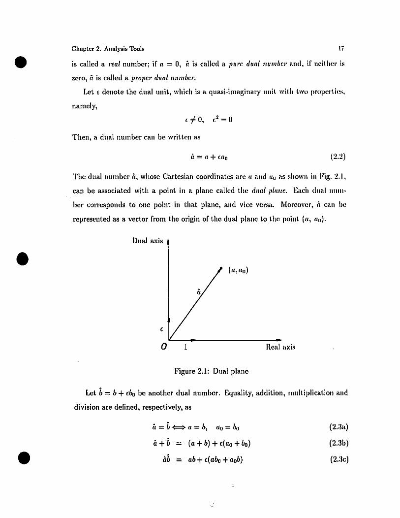
The dual number â, whose Cartesian coordinates are a and ao as shown in Fig. 2.\,

can be associated with a point in a plane called the dual /J/tme. Each dual nnnl­

bel' corresponds to one point in that plane, and vice versa. l\'loreover, il can be

represc'nted as a vedor from the origin of the dual plane to the point (a, au).

Dual axis

•(

1

(a,au)

Real axis

Figure 2.1: Dual plane

Let b= b+ (bo be another dual number. Equality, addition, Illult.iplication and

division arc deflned, respectively, as

•â = b<==> a = b, ao = be

â +b - (a +b) + ((ao +bol

âb = ab + ((abe +aob)

(2.:la)

(2.:lb)

(2.:lc)

•Chaptcr 2. Analysi. '1'001. 18

(2.3d)

From e'l.(2.3d) it i. ohvious that division hy a pure dual is not defined. Hence, dual

nU1llbc,·.~ do nol Jorm a field.

Ali formai operations involving dual numhers arc identical to those of ordinary

algehra while taking into account that (2 = (3 = ... = O. The series exp"nsion of an

analytic fundion of a dual numher is of great importance, i.e.,

The dual angle Ôbetween two skew lines .cl and .c2, introduced by Study (1903), is

dcfined as

•

• dJ(a)J(a) = J(a +wo) = J(a) +wo-l-

ca

where ail higher terms vanish hecause of the foregoing property of (.

2.2.1 Dual Quantities

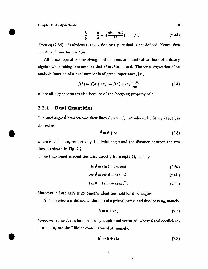
Ô= 0 +(s

(2.4)

(2.5)

where 0 and o. arc, respedively, the twist angle and the distance hetween the two

Iines, as shown in Fig. 2.2.

Three t.rigonometric identities arise directly from eq.(2.4), namely,

sin Ô= sin 0 +(s cos 0

cos Ô= cos 0 - (ssinO

tan Ô= tan 0 +(s sec2 0

(2.6a)

(2.6b)

(2.6c)

l\'loreover, ail ordinary trigonometric identities hold for dual angles.

A lirtrll vcetOl' â is defined as the sum of a primaI part a and dual part 80, namely,

Morcaver, a line A can be specified by a unit dual vector a", whose 6 real coefficients

in a and au are the Pliicker coordinates of A, namely,

• a" = a+(8o

(2.7)

(2,8)

•Chapt"r 2. Analysis Tools

s

Figure 2.2: Dual angle beLween two skew Hnes

19

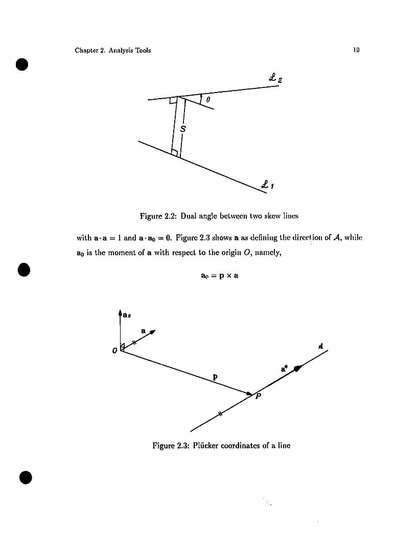
•with a·a = 1 and a·au = O. Figure 2.3 shows a as defining the diredion of A, while

an is the moment of a with respect to the origin 0, namcly,

a.

o

•Figure 2.3: Plücker coordinates of a line

Quaternions were introduced by Hamilton (1844). They have recently played a

significant role in several areas of science and engineering, namely, in differential

geometry, in analysis and synthesis of mechanisms and machines, simulation of par­

ticle motion in molecular physics, and in the formulation of the relativistic equation

of motion (Agrawal, 1987). Funda and Paul have shown that quaternions offer the

most efficient alternative among point transformation formalisms (Funda and Paul,

I!J90). However, they hava not received wide publicity in the area of kinematics and

dyn;lmics of mechanisms. This is mainly because quaternion algebra is complicated

and leads to tedious operations.

The word quaternion is derived from the Latin word quaterni and means a set of

four. It is a linear combination of four quaternion units, 1, i, j and k, namely,

•

•

CllIlptcr 2. Analysis Tools

2.2.2 Quaternions

with the definitions

q = cl +ai +bj +ek

.. k·k . k' .IJ = ,J =l, 1 =J

20

(2.9)

Pre-multiplying both sides of ij = k, jk =i and ki = j by i, j and k, respectively,

leads to

·k '" k kj .1 = -J, JI = -, = -1

Moreover, cl, a, band c are ail real numbers. The three quaternion units i,j and k

can be considered as orthogonal unit vectors with respect to the scalar produet. For

this reason i,j and k are also identified as an orthogonal triad of unit vectors in a

3-dimensional Euclidean space.

A quaternion consists of two parts, the scalar part s, and the vector part v,

namely,• q=s+v (2.10a)

•

•

Chaptc' 2. Analysis Toois

where

s::d

v:: ai +bj +ck

The n01"m of il quaternion is defined as

where k(q) is called the conjugate of q, defined as

k(q)::s-v

Then, eq.(2.l1) leads to

N = ve(l +a2 +b2 +c2

Furthermore, the reciprocal of a quaternion is defined as

(1_ 1 = k(q)- N2

and, as a result, wc have

21

(2.10h)

(2.lIk)

(2.11 )

(2.12)

(2.1 :1)

(2.11i)

A unit quaternion q" is a quaternion whose norm is unity, and takes on the general

form

and s is the unit vector representing the axis of the unit quaternion e(; it is given IL~

•

where

q" = cos 0 +ssin 0

dcos 0 =-

N~~~~. va2 + b2 +c2

Slll 0 = N

s = _a7i=;;+~bj~+~ck="va2 +b2 +c2

(2.IHa)

(2. Wb)

•Chaptcr 2. Analysis Tools

2.2.3 The Product of 'l'wo Vectors

Civen two unit vectors a and h, their produet ab, in this arder, is defined as

ab ;: -a· b + a x b

= - cos 0 + s sin 0

22

(2.17)

•

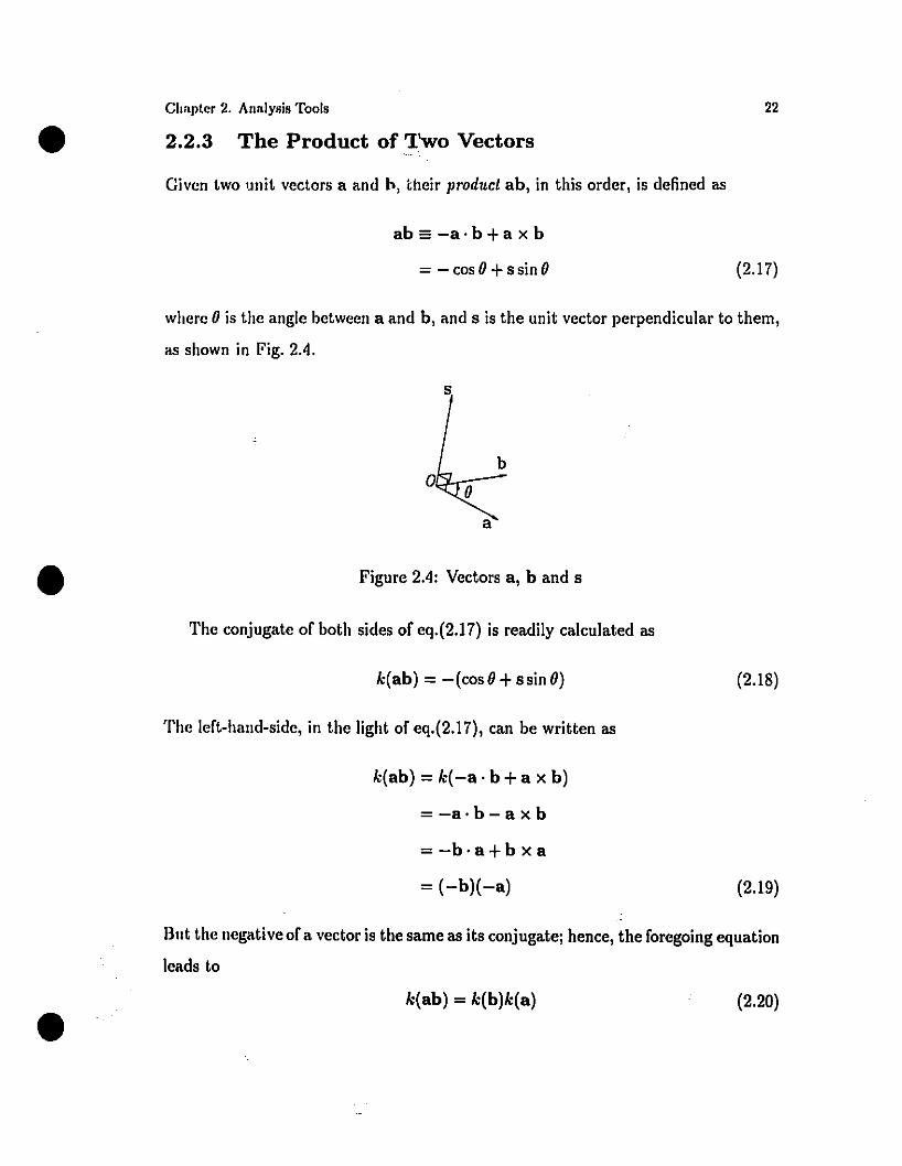
where 0 is the angle between a and b, and s is the unit vector perpendicular to them,

as shown in Fig. 2.4.

Figure 2.4: Vectors a, band s

The conjugate of both sides of eq.(2.l7) is readily calculated as

Bllt the lIegative of a vector is the same as its cOlljugatej hence, the foregoing equation

leads to

•

k(ab) = -(cosO+ssinO)

The left-halld-side, in the light of eq.(2.l7), can be written as

k(ab) = k(-a . b + a x b)

= -a· b- a x b

= -b·a+b xa

= (-b)(-a)

k(ab) = k(b)k(a)

(2.18)

(2.19)

(2.20)

•Chapter 2. Analysis Tools 23

Substitution of the value of k(ab) from eq.(2.20) into eq.(2.18), and'noting that the

right-hand-side of the latter is equal to -q", leads to

But, from eq.(2.14), we have

k(b)k(a) = -q"

k(a) = a-1

(2.21 )

(2.22)

Substitution of the value of k(a) from eq.(2.22) into eq.(2.21), with the faet that

k(b) is equal to -b,yields'"

q" = ba- I (2.23)

Furthermore, post-multiplying both sides of the foregoing equation by a yields

q"a= b (2.24)

(2.25a)

•whieh implies that a unit quaternion q" is a rotation opemtor. It rotates a vedor

a through an angle 0 about an axis s, called the quaternion axis that interseds the

vector at right angles, as shown in Fig. 2.4. Morcover, this operation preserves the

Euclidean norm of vectors.

The relation between a unit quaternion q" and the corresponding rotation matrix

Q follows directiy from definitions (2.16a) and (2.16b), namely,

1q" = 2[tr(Q) - 1] + vect(Q)

where tr(Q) and vect(Q) are the linear invariants of Q , as defined in (Angeles, 1988)

as

in which s, 0 and S are the axis of rotation, the rotation angle and the cross-product

matrix of vector s.•

tr(Q)=1+2cosO

vect(Q) = sin Os

Moreover, Q is given in an invariant form in this reference as

Q =ssT + cos 0(1 - ssT) + sin OS

(2.25b)

(2.25c)

(2.25d)

•Chllptcr 2. Anlllysis Tools

2.2.4 Dual Quaternions

24

The quaternion concept was combined with that of dual numbers by Yang (1963)

to producc the dual quaternion. Moreover, he applied the latter to analyze four-bar

linkages. Recently, Funda and Paul showed that dual quaternions provide the most

compact and computationally efficient formalism for motion in parallel and seriai

screw computations (Funda and Paul, 1990).

A dual quaternion q is a quaternion with dual components, namely

(2.26)

where d, êt, band ê are dual numbers. Simitar to an ordinary quaternion, a dual

quatemion con~ists of two parts, the scalar part S, and the vector part v, namely,

q=s+v (2.27a)

• where

s==d (2.27b)

v == âi+bj+êk (2.27c)

Moreover, the conjugate of a dual quaternion is defined as

'.

k(q) == s-v

white the norm of n dual quaternion is defined as

Furthermore, the reciprocal of a dual quaternion is defined as

and, as a result, we have

(2.28)

(2.29)

(2.30)

(2.31)

•Chapter 2. Analysis Tools

A unit dual quaternion ij" is a dual quaternion with norl11 equal to unit,y, uame1y,

25

where

ij" = cos Ô+5 siu Ô

• cicosO = ...,..

N.' y'-â-2 -+-:b"-2-+-c-'2

smO = .N

(2.32a)

•

and hence, s" represents the Pliicker coordiuates of the axis of the unit dual <Iuater­

nion ij', which is given as

(2.:l2b)

2.2.5 The Produet of Two Lines

Given the Pliicker coordinates of two tines A and B in dual-veetor fOI"I11, a' and b',

the product of A by B, in this order, is defined as the product of a' by b', in t.he

corresponding order, namely,

where

a'b' =-a' . b' +a' x b'

a'· b' = a· b +c(a· bo 1- ao· b) = cos Ô

a' x b' = a x b +c(a x bo+ao x b) = s· sin Ô

(2.:l3a)

(2.:J3b)

(2.:l3c)

•

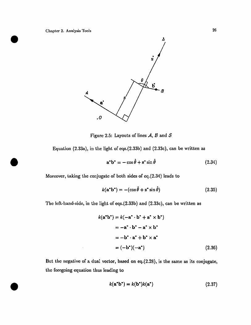
in which s' is an unit duall'ector representing the Pliicker coordinates of the comrnon

perpendicular between a' and b·. Moreover, Ôis given as

ô= 0 +cs

in which 0 is the twist angle and s is the distance between the two tines, respcetively,

as shown in Fig. 2.5.

i.'.

But thc IIcgativc of a dual vedor, based on eq.(2.28), is the same as its conjugate,

thc foregoing equation thus leading to

•

•

•

Chaptcr 2. Analysis '1'001.

Figure 2.5: Layouts of lines A, Band S

Equation (2.33a), in the light of eqs.(2.33b) and (2.33c), can be written as

a·b· = -cosÔ+s·sinÔ

Moreover, taking the conjugate of both sides of eq.(2.34) leads to

k(a·b·) = -(cos Ô+ s· sin Ô)

The Icft-hand-side, in thc light of cqs.(2.33b) and (2.33c), can be written as

k(a·b·) = k(-a· . b· +a· x b·)

= -a· . b· - a· x b·

= -b· . a· +b· x a·

= (-b·)(-a·)

k(a·b·) = k(b·)k(a·)

26

(2.34)

(2.35)

(2.36)

(2.37)

•Chapter 2. Analysis Toois

Substitution of the value of k(a"b") from eq.(2.3i) into eq.(2.35), with the faet. that

the right-hand-side of the latter is equal to -q", leads to

But, from eq.(2.30), we have

k(b")k(a") = -q"

k(a") = (a"t l

(2.:18)

(2.:I!I)

Substituting the value of k(a") froIn eq.(2.39) into eq.(2.38), and IlOting t.hat k(b")

is equal to -b", we obtain

Ir = ba- I

Post-multiplying both sides of the above equation by a" leads to

(2AO)

(2A 1)

•

•

which impties that a unit dual quaternion q" is a scrcw 0lJCI'/LlOl', It rotates a tine

A through an angle 0 about an axis S that intersects the tine at right angles, and

stides it along that tine through a distance s, as shown in Fig. 2.5,

As explained cartier, the main drawback of <Iuaternions is that thcir algebra is

quite involved, the complexity rclated to that of dual quaternions being even more

50. To overcome this obstacle, the author implemented some user-defined functiollH

in a MATHEMATICA environment to handle computations such as the product of

two tines, the product of two dual quaternbns, and the product of a tille by a dual

quaternion, to be used in Chapter 4.

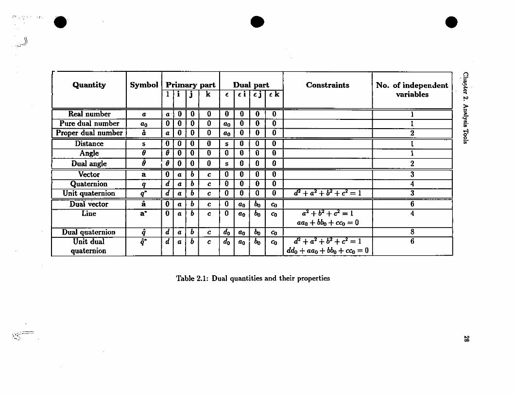
All the dual quantitics and their properties are summarized in Table 2.1.

2.2.6 Dual Screw Matrices

Here, wc combine the concept of rotation matrix with that of dual numbers, and

will find a dual scrcw matriz in an invariant form. Let us define two Iines A and S

in dual-vector form as a" and s", respectively. Line A rotates through an angle 0

...-; . ~

\~J• • •

>::.:::.::=.:.-:

Quantity Symbol Primary part Dual part Constraints No. of indepenJent1 i j k f fi d fk variables

Real number a a· 0 0 0 0 0 0 0 1Pure dual number ao 0 0 0 0 ao 0 0 0 1

Proper dual number â a 0 0 0 ao 0 0 0 2Distance s 0 0 0 0 s 0 0 0 1

Angle 0 0 0 0 0 0 0 0 0 1Dual angle 0 0 0 0 0 s 0 0 0 2

Vector a 0 a b c 0 0 0 0 3Quaternion q d a b c 0 0 0 0 4

Unit quaternion q* d a b c 0 0 0 0 cP +a' +b' +c' - 1 3

Dual vector â 0 a b c 0 ao bo Co 6Line a* 0 a b c 0 ao bo Co a'+b'+c = 1 4

aao +bbo +CCo = 0Dual quaternion q d a b c do ao bo Co 8

Unit dual q* d a b c do ao bo Co dl +a2 +b' +c2 = 1 6quaternion ddo+aao +bbo +CCo = 0

Table 2.1: Dual quantities and their properties

()

';.~

!'O>"!!.'ai!O"

b'o..

'"00

•

•

Chapter 2. Analysis Toois

(8

s'

s

29

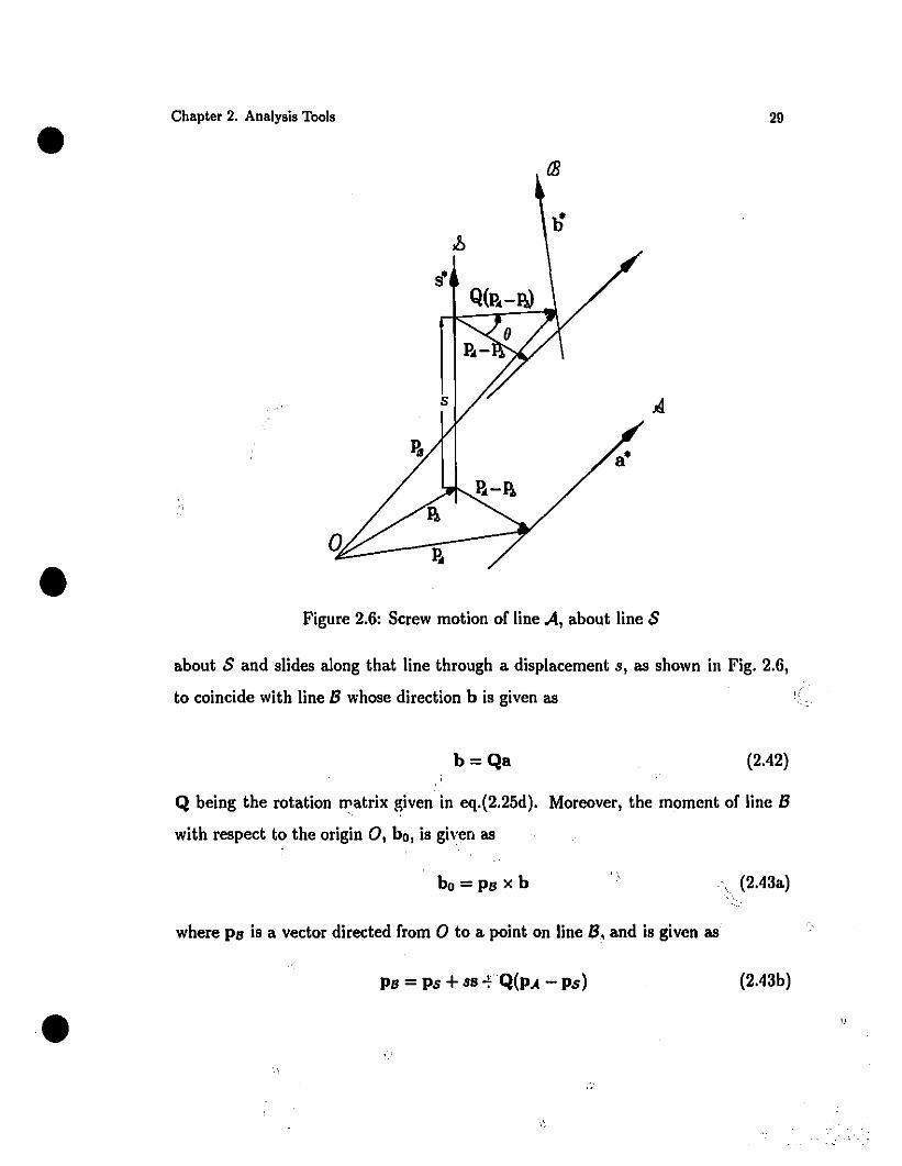
Figure 2.6: Screw motion of Hne A, about Hne S

about Sand sHdes a10ng that Hne through a displacement s, as shown in Fig. 2.6,

to coincide with Hne B whose direction b is given as

b=Qa (2.42)

Q being the rotation lPatrix given in eq.(2.25d). Moreover, the moment of Hne B

with respect to the origin 0, bD, is gh;en as

•

bD =PB X b

where PB is a vector directed from 0 to a point on Hne B, and is given as

PB =PS +S8 +Q(p.A - Ps)

(2.43a)

(2.43b)

Substituting the values of band P8 from eqs.(2.42) and (2.43b) into eq.(2.43a) [eads

to•Chapter 2. Analysis Tools

bo = [ps + ss + Q(p.A - Psi] x (Qa)

Equation (2.44), upon expansion, yields

bo =Ps x (Qa) + ss x (Qa) + (Qp.A) x (Qa) - (Qps) x (Qa)

30

(2.44)

(2.45a)

Upon substitution of the value of Q from eq.(2.25d) into eq.(2.45a) and expansion,

the first term of the foregoing equation leads to

PS x (Qa) = (ps >( s)sTa + cosO(ps x a) - cosO(ps x s)STa + sin O[ps x (5 x a)]

= sosTa + cos O(ps x a) - cosOsosTa +sin O[(p~a)s - (p~s)a] (2.45b)

•Sirnilarly, for the second, third and fourth terms of eq.(2.45a), we have

sS x (Qa) = s(s x s)sTa + s cos 0(5 x a) - s cos 0(5 X s)STa

+s sin 0[5 x (5 x a)]

=s cos 0(5 x a) +ssinO[(sTa)s - (sTs)a]

(Qp.A) x (Qa) = Q(p.A x a) = QlIo

(Qps) x (Qa) =Q(ps x a)

= ssT(pS x a) + cos O(Ps x a) - cos O(ssT)(ps x a)

+ sin Ols x (PS x a)]

=-ss;fa + cos O(Ps x a) + cos Oss;fa

+sinO[(sTa)ps - (sTps)a]

(2.45c)

(2.45d)

(2.45e)

•

Substituting the values of ps x (Qa), ss x (Qa), (Qp.A) x (Qa) and (Qps) x (Qa)

from eqs.(2.45b-e) into eq.(2.45a), upon simplification, yields

•Chaptcr 2. Analysis Tools

bo = Qao + (5051' + sS6)a - ssin 0(1- ssT)a - cosO(sosf + ss~')a +

sin O[(p~a)s - (51'a)psJ +s cos 0(5 x a)

= Qao + [(5051' + 556) - ssinO(I- 551') - cosO(Sosl' + ss~') +

sin OSo + s cos OSJa

:11

(2.'16)

in which So is the cross-product matrix of vector 50. From eqs.(2,42) and (2,4li), b­

can be written as

Wc have thus shown that a dual screw matrix can readily be derived by changing the

real quantities of the rotation matrix of eq,(2.25d) into dual quantities. The saille

is true for its Iinear invariants, namely, tr(Q) and veet(Q), as we show below. From

the invariant representations of the dual screw matrix, eCI.(2,48b), it is clear that the

first two terms of Q, namely, 5'5'1' and cos Ô(1 - s·s·'I') arc symmetric, while the

last term is skew-symmetric. Hence

•

•

b' =b + fbo = Qa + fQao + f[(SoSI' + 556) - s sin 0(1 - ssl')

- cos !J(soST + ss~') + sin OSo + s cos OSJa

Equation (2.4ï) leads to a simple form, namcly,

b' = Qa'

where Q is the dual screw matrix in invariant form, i. e.,

Q = 5'5"1' +cos Ô(1 - 5'5"1') +sin ÔS

with s·T and Sare defined as

.'1' '1' 7'5 =5 +(50

S=, '5 + (So

tr(Q) = tr[s·s·7· +cosÔ(l- s·s·T)J =) +2cosÔ

vect(Q) = vect(sin ÔS) = sin ÔS'

(2Aï)

(2A8a)

(2,48b)

(2,48c)

(2,48d)

(2,49a)

(2,49b)

Therefore, the relation between a unit dual quaternion ê( and the corresponding dual

screw matrix Q follows directly from definitions (2.32a) and (2.32b), namely,•Chnptcr 2. Annly.i. '1'001.

1. .ê( = 2"[tr(Q) - 1] +vect(Q)

32

(2.50)

•

Moreover, eqs.(2A9a) and (2A9b) should find extensive applications in the realm of

motion determination whereby the displacement of sorne Iines of a rigid body are

given, and, from these, the screw parameters are to be determined.

2.3 Spatial Trigonometry

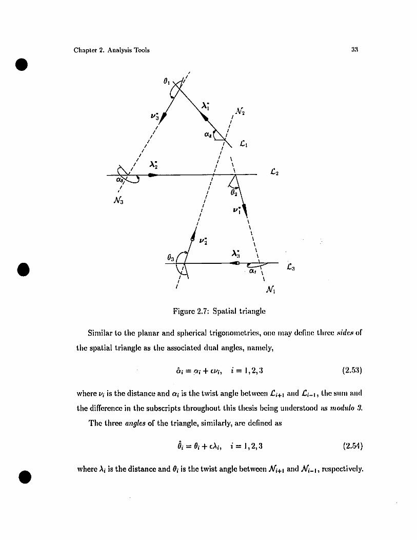
2.3.1 Spatial Triangle

A spatial triangle consists of three skew lines in space and their three common

perpendiculars, as depicted in Fig. 2.7. In that figure, the three Iines are labelled

{(,i n, thcir corre,'pondinl~ normals being {JI!; n, where NI is the common normal

between lincs (,2 and (,3, N2 is that between (,1 and (,3, with a similar definition for

N3 • The Iines are given by the three unit dual vectors {~i n, defined as

~i == ~i + (~0Î1 i = 1,2, 3 (2.51)

where ~i and ~Oi arc, respectively, the direction and the moment vectors of (,i about

origin.

Moreover, the thrcc cornmon perpendiculars of the foregoing Hnes, {JI!; n, are

given by the thrcc unit dual vectors { /Ii n, defined as

/Ii == /Ii + (/lOi, i = 1,2,3 (2.52)

•with /Ii and /lOi representing, respectively, the direction and the moment vectors of

line Ni about the origin.

•Chaplcr 2. Anal~'.i. 1'001•

À"N2

1

11

1 11 1

1 oc. 11 1 .cl1

1 1

1 11 \1

À" 11 1 \

1 21 \ .c2

11

11

N31

111

11 \1

\\

V" \2 \

À; \

03\

• OC, .c:l\\

NI

Figure 2.7: Spatial triangle

Similar to the planaI' and spherical trigonometril)S, one may deline t.hl'ee "i,{"" of

the spatial triangle as the associated dual angles, namely,

âi = !;fi +(/Ii, i = 1,2, a (2.5:1)

where /Ji is the distance and Cli is the twist angle between .ci+1 and .ci_l, the Sil 111 and

the difference in the subscripts throughout this thesis bcing understood ;L~ mO,{lIlo .'J.

The three (lllgics of the triangle, similarly, arc delined ;L~

where ~i is the distance and Oi is the twist angle between N i+1 and Ni-l, respectively.•Ôi = Oi + (~i, i = 1,2,3 (2.M)

•Chapt"'~. A"alysis Tools

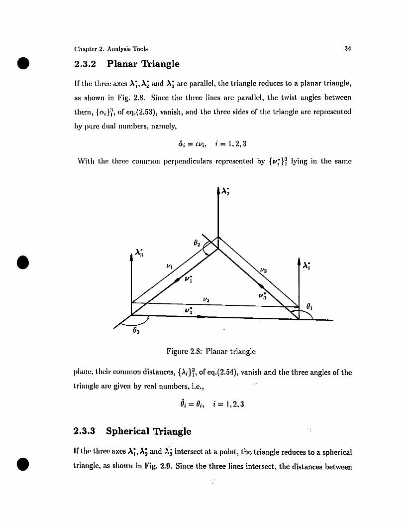
2.3.2 Planar Triangle

34

•

•

If the three axes À;, Ài and À; arc paralld, the triangle reduces to a planar triangle,

1,", shown in Fig. 2.8. Since the three lines arc parallel, the twist angles between

t.hem, {Oirl, of eq.(:2.5a), vanish, and t.he t.hree sides of the triangle arc represent.ed

hy pure dual nUlllhers, namely,

âi=CVi, i=1,2,a

Wit.h t.he t.hree COllll1lon perpendiculars represented hy {viH Iying in the saille

À"2

Figure 2.8: Plauar triangle

plane, their colllmon distances, Pin, of eq.(2.54), vanish and the three angles of the

triangle are given by real nUl1lbers, i.e.,

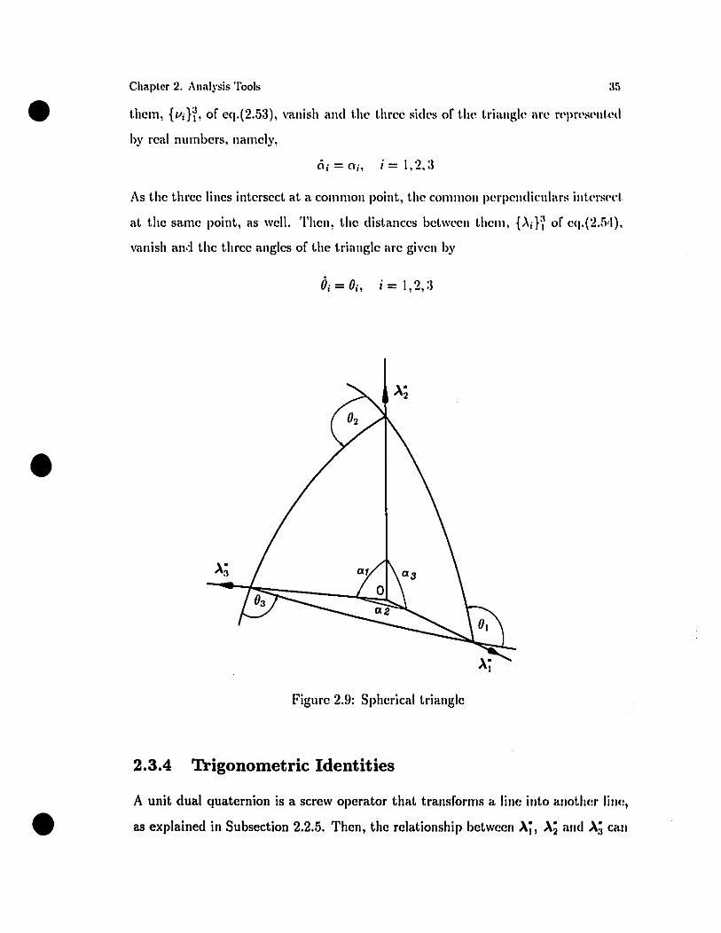
2.3.3 Spherical Triangle

If t.he tllI'ce axes À;, À; and X; intersect at a point, the triangle reduces ta a spherical

triangle, as sholVn in Fig. 2.9. Since the three lines intersect, the distances between

•

•

•

Chapter 2. Anal)'sis Tools

them, {Vin, of eq.(2.53), vanish and the three sides of the triangle arc represented

by real numbers, namely,

6; = ni, i=I,2~3

As the three lines intersecl at a coml1lon point, the coml1lou pcrpendknlars intersl'd,

at the same point, as weil. Then, the distances betwccn thel1l, Pin of eq.(:UH),

vanish and the three angles of the triangle arc given by

Ôi = Oi, i = 1,2,:3

Figure 2.9: Spherical triangle

2.3.4 Trigonometrie Identities

A unit dual quaternion is a screw operator that transforms a line into another Iillc,

as explained in Subsection 2.2.5. Then, the relationship bclween ~i, ~; alld ~; cali

•Chapt", ~. A'IIllysis Toois

he ex presse" as

'" .. ,."3 = V, "2

where ";, for j = 1,2,:1, is a unit dnal quaternion, given as

.. . + .' .IIi = casai Il; sinaï

SnbsLitnting the value of Àj from eq.(2.55c) into eq.(2.5.5a) yields

36

( ? -- )_.uua

(2 ..55b)

(2 ..55c)

(2.55d)

(2.56)

•Moreover, snbstiLnting the value of À; from eq.(2.55b) into eq.(2.56), upon simplifi-

cation, leads ta

(2.57)

The foregoing identity is calicd the angu/m' c/oSU1'e equation for spatial triangles; it

states that the three consecutive screw motions of Àj, represented by vi, vi and vj,tl'ansforll1s Àj, via the intermediate poses À; and Àj, back into itself.

Sill1ilarly, the side c/osul'e equation for spatial triangles transforms IIi, via the

intel'JlIediate poses Il; and IIj, back into itself, namcly,

where ~;, for i = 1,2,3, is a unit dual quaternion, given as

~i = cos Ôj +Ài sin Ôj

(2.58a)

(2.58b)

•One lI1ay conclude from eqs.(2.57) and (2.58a) the following spatial trigonometric

identit.ies (Yang, 1963):

Sine law:

(2.59)

•Chapter 2. Anal)'sis Toois

eosine 1aws:

cos ô. = cos â 2 cos â" - sin â2 sin â" cos Ô\

cos Ô" = cos Ô\ cos Ô2 - cos ci:. sin Ô\ sin Ô2

- sin ô\ cos Ô" = sin â2 cos Ô:l +cos Ô2 sin ô" cos Ô1

- sin Ô2 sin Ô" = sin Ô\ cos Ô2 +cos â:l cos Ô. sin Ô2

(:UlOal

(2'(lOl>1

(2.lilkl

(2.lilldl

•

•

The foregoing identities ho1d for spherical triangles. Indeed, if n is challged 1.0 ('l,

these identities become the sine and cosine laws of spherical triangles. MOI'"ove'r, fol'

planaI' triangles, the sine law and the cosine law l'l'duce 1.0 the e\elllcnt.ary sille and

cosine 1aws of planaI' trigonometry.

•

•

•

Chapter 3

Parallel Manipulators

3.1 Introduction

Here, we introduce planar and spherical DT manipulators and, based on spatial

tl'igonometry, which was introduced in Chapter 2, wc generalize the concept of DT

manipulators to that of spatial DT manipulators. Moreover, two general classes of

plana,' manipulators are given, wherein the first class contains 20 manipulator types

and the second contains four types. For the sake of completeness, the spherical

3-RRR manipulator is included as weil.

3.2 Planar Manipulators

Planar tasks, whereby objects undergo two independent translations and one rota­

Hon about an axis perpendicular to the plane of the two translations, are common

in manufacturing operations. These can be accomplished by planar parallel manip­

ulators that consist of two rigid bodies connected to each other via several cop\anar

legs.

.One of the general classes of planar parallel manipulators consists of two clements,

lIiunC:y the base ('P) and the moving (Q) plates, connected by three legs, each with

thrcc degre'ls of freedom. Thes!' will be called three-legged (3L) manipulators. The

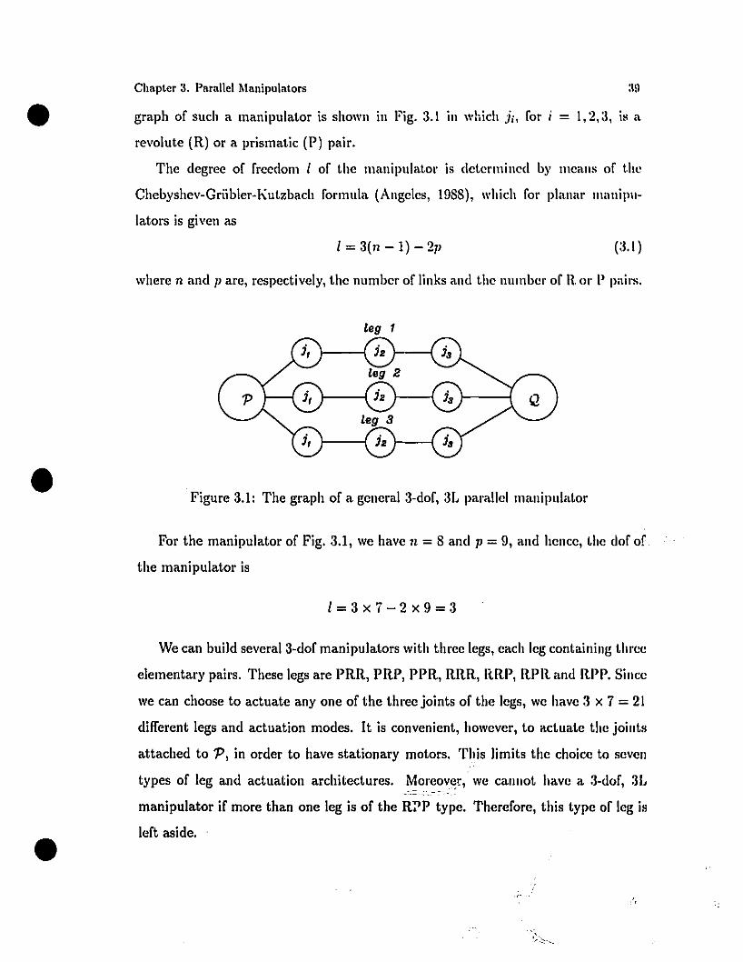
•Chaptcr 3. Parallel Manipulators

graph of such a manipulator is shown in Fig. 3.1 in which ii, for i = 1,2,3, is a

revolute (R) or a prismatic (P) pair.

The degree of freedom 1 of the manipulator is determincd by meatls of thc

Chebyshev-Griibler-Kutzbach formula (Angeles, 1988), which for planaI' nmnipu­

lators is given as

1= 3(n - 1) - 2]1 (3.1 )

•

•

where n and ]1 are, respectively, the number of links and the ntlmbci' of Il or l' pairs.

leg 1

Figure 3.1: The graph of a general 3-dof, 3L parallel manipulator

For the manipulator of Fig. 3.1, we have 11 = 8 and ]1 = 9, and hencc, the dof of

the manipulator is

1=3x7-2x9=3

We can build several 3-dof manipulators with three legs, each leg containing three

elementary pairs. These legs are pRR, l'RI', pPR, RRR, RRp, RPR and Rpl'. Since

we can choose 1.0 actuate any one of the three joints of the legs, we have 3 x 7 = 21

different legs and actuation modes. It is convenient, however, 1.0 actuate the joints

attached 1.0 P, in order 1.0 have stationary motors. This limits the choice to seven

types of leg and actuation architectures. rvt0reov~r, we canllot have a 3-dof, 3L

manipulator if more than one leg is of the R:'p type. Therefore, this type of leg is

left aside.

Lel us ch..,sify the remaining legs into two categories, based on their third joints.

'l'hase legs aUached ta Q with a revolute joint form the lirst eategory, i.e., PRR,

PPR, RRR and RPR. The 31. manipulators construded with these legs are ealled

lIIanipulators of dass A. Moreover, those legs aUached 1.0 Q with a prismatie joint

form the legs of another 31. parallel manipulator dass that will be ealled class l3.

The joinl. sequences for the legs are PRP and RRP.

•Chapter:l. l'aralld Ma"ip"intors 40

•

•

3.2.1 3-DOF Manipulators of Class Â

As explained above, the dass-A manipulator has three legs and ean be built with

allY thl'cp' combinations of four types of legs, namely, PRR, PPR, RRR and RPR.

Then, the nllmber of manipulators in this dass is given as

·1

11 = ~)4 - i + l)i = 20i=1

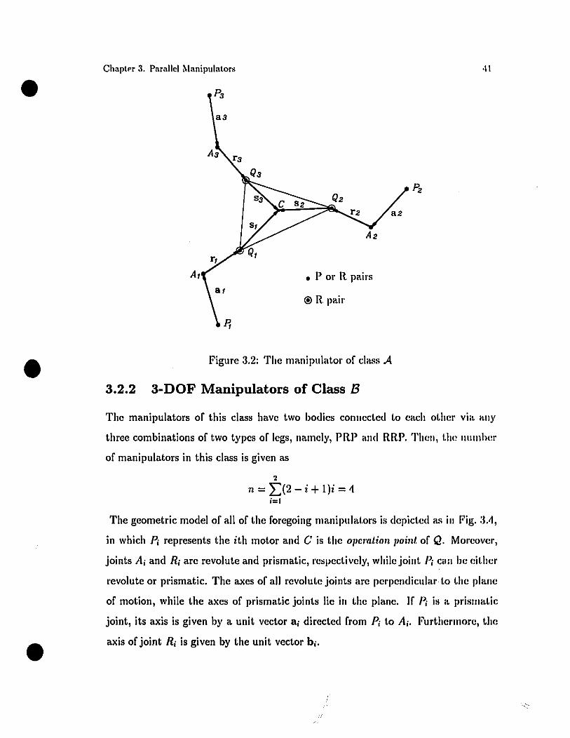
The geometric moclel of ail of the foregoing manipulators is depided as in Fig. 3.2,

in whieh Pi represents the ith motor and C is the o/lemtion /loint of Q. Moreover,

joint, Qi is a revolute, while joints Pi and Ai can be either revolute or prismatic. The

axes of ail revolute joints are perpendicular to the plane of motion, while the axes

of l'rismatic joints lie in the plane. If Pi is a prismatic joint, its axis is given by a

vect.or ai directc:d from Pi ta Ai. Similal'ly, if Ai is a prismatic joint, its axis is given

by a vedor ri directed from Ai to Qi.

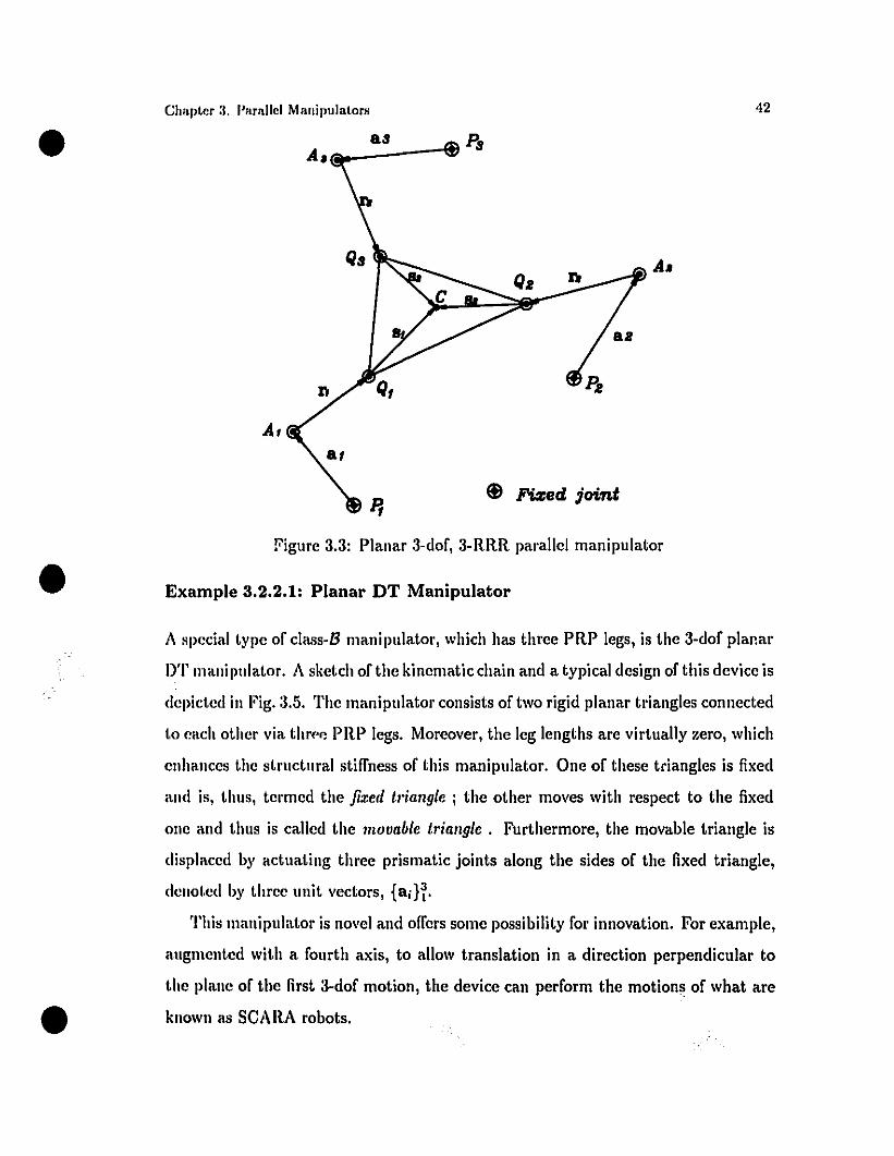
Example 3.2.1.1: Planar 3-RRR Manipulator

An exalllple of the manipulator of dass A is the planaI' 3-RRR manipulator, which

has been the subjed of extensive research (Hunt, 1983j Mohamed, 1983j Gosselin,

I!J88j Gosselin and Angeles, 1989j Gosselin and Sefrioui, 1991). This manipulator is

constl'uct.ed with two bodies, 'P and Q, conneeted to each othCl via three RRR legs,

as depict.ed in Fig. 3.3. Morcaver, ail three motors Pi are lixed to the ground.

Chaptpr 3. Parallcl Manipulators

3-DOF Manipulators of Class B

·11

A2

• l'or R pairs

@ R pair

Figure 3.2: The maniplliatoi' of c1ass A

At

3.2.2•

•

The manipulators of this c1ass have two bodies connected to each other via any

three combinations of two types of legs, namely, l'RI' and RRp. Then, the nnmher

of manipulators in this c1ass is given as

2

n = ~(2 - i + l)i = 1\i=1

•

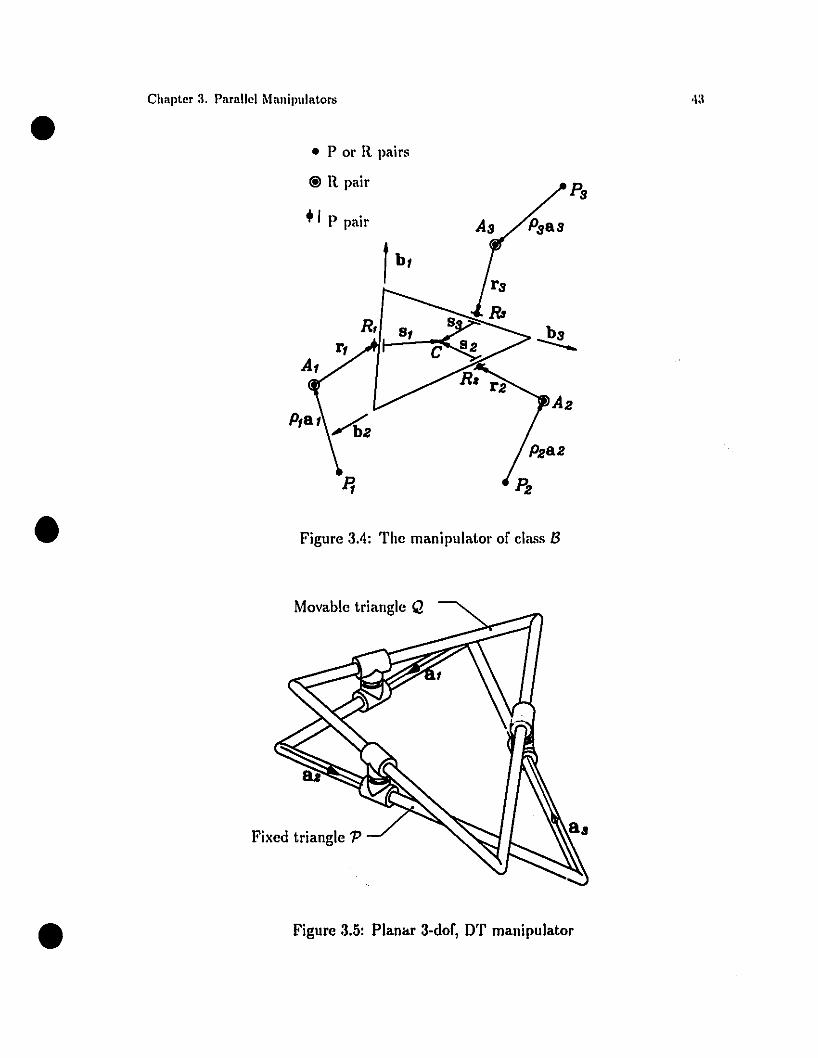
The geometric model of ail of the foregoing manipnlal.ors is depicted as in Fig. :tl\,

in which Pi represents the ith motor and C is the o/lcmlion /loint of Q. MOl'eover,

joints Ai and Ri are l'evolute and prismatic, respectively, while joint Pi can be cit.hel·

revolute or prismatic. The axes of ail revolute joints are perpendiclliar to the plane

of motion, while the axes of prismatic joints lie in the plane. If Pi is a prismatic

joint, its axis is given by a unit vector ai directed from Pi to Ai. Furthermore, the

axis of joint Ri is given by the unit vector bi.

•

•

Chapter:l. Parullel Malliplliators

a8 Rr..-_---1!' "8

A.

A,

$ Fia:ed. joint

figure 3.3: PlanaI' 3-dof, 3-RRR parallel manipulator

Example 3.2.2.1: PIanar DT Manipulator

42

•

A special type of c1ass-B manipulator, which has three PRP legs, is the 3-dof planaI'

DT mani pulator. A sketch of the kinematic chain and a typical design of this device is

dcpictcd in Fig. 3.5. The manipulator consists of two rigid planaI' triangles connected

1.0 each othcr via thrpp. PRP legs. Moreover, the leg lengths arc virtually zero, which

enhances thc structural stilfness of this manipulator. One of these triangles is fixed

and is, thus, termed the flxed Il'iangle ; the other moves with respect to the fixed

one and thus is called the lIIouable triangle. Furthermore, the movable triangle is

displaced by actuating three prismatic joints along the sides of the fixed triangle,

dcnoted by three unit vectors, {aiHoThis manipulator is novcl and olfers sorne possibility for innovation. For example,

augmented with a fourth axis, to allow translation in a direction perpendicular to

the plane of the first 3-dof motion, the device can perform the motions of what are

known as SCARA robots.

•

•

•

Chapter 3. Parallcl Mnnipulators

• P or Il. pairs

@ Il. pair

+1 P pair

R, s,f

Figure 3.4: The manipulator of dass B

Movable triangle Q

Fixed triangle 'P

Figure 3.5: Planar 3-dof, DT manipulator

CI"'pler :1. l'''rallel Manipulalors

• 3.3 Spherical Manipulators

44

•

•

Spherical motion allows the arbitrary orientation of workpieccs in 3D space. Herc,

two types of spherical parallcl manipulators, namely, the spherical 3-RRR and the

spherical DT rnanipulators, arc inclnded. Both of these devices consist of two bodies

connected by three 3-dof legs, the graph of such a devicc being that of Fig. 3.1. More­

over, the dof of spherical manipulators is determined by means of the Chebyshev­

Griibler-J(utzhach formula, as given in eq.(3.11. Here we have Il = 8, ]J = 9 and,

agai n, the dof, l, of the device is

1= 3(8 - 1) - 2 x 9 = 3

3.3.1 Spherical 3-DOF, 3-RRR Manipulator

This manipulator consists of two bodies connected by three RRR legs, as shown

in Fig. 3.6. Moreover, three actuators are attached to the base and rotate the

links connected to the base about {uiH. Similar to its planaI' counterpart, this

manipulator is weil documented in the research Iiterature (Cox and Tesar, 1989;

Craver, 1989; Gosselin and Angeles, 1989; Gosselin et a!., 1994a, 1994b; Gosselin

and Lavoic, 1993).

3.3.2 Spherical 3-DOF, DT Manipulator

The spherical 3-dof, DT manipulator consists of two spherical triangles connected

by thrcc legs. Similar to its planaI' counterpart, itr leg lengths are virtually zero,

which makes it particularly stiff. One of these triangles is fixed, and is thus termed

the fixed triangle; the other moves with respect to the fixed one, and thus is called

the movable triangle. Morcaver, the movable triangle is driven by three actuators

placed along the sides of the;iixed triangle, with actuated-joint variables {Jld~.

•

•

Chapter 3. Parallel Manipulators

u.

Q,

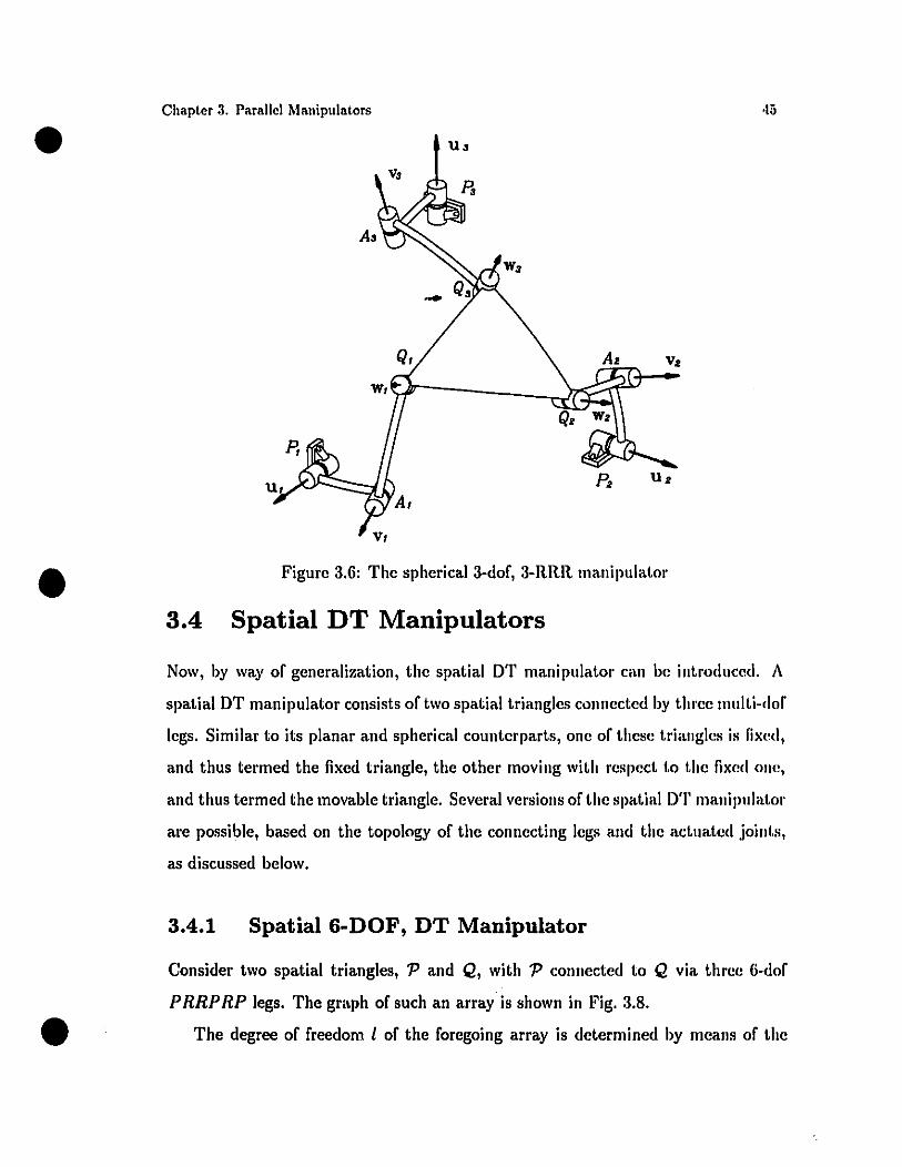
Figure 3.6: The spherical 3-dor, 3-RRR lllaniplIlator

·15

3.4 Spatial DT Manipulators

Now, by way or generalization, the spatial DT lllaniplliator can be int,rodllccd. A

spatial DT lllaniplliator consists or two spatial triangles connected by three llllliti-rior

legs. Silllilar to its planar and spherical cOlinterparts, one or these triallgles is fixed,

and thlls terllled the fixed triangle, the other lllovillg with respect t.o the fixed Olle,

and thus termed the movable triangle. Several versions or the spat.ial DT lllaniplliator

are possible, based on the t.opology or the connecting legs and the aetllated joint.s,

as discussed below.

3.4.1 Spatial 6·DOF, DT Manipulator

•Consider two spatial triangles, 'P and Q, with 'P connected to Q via three 6-dor

PRRPRP legs. The gmph or such an array is shown in Fig. 3.8.

The degree or rrcedom 1 or the roregoing array is determincd by means or the

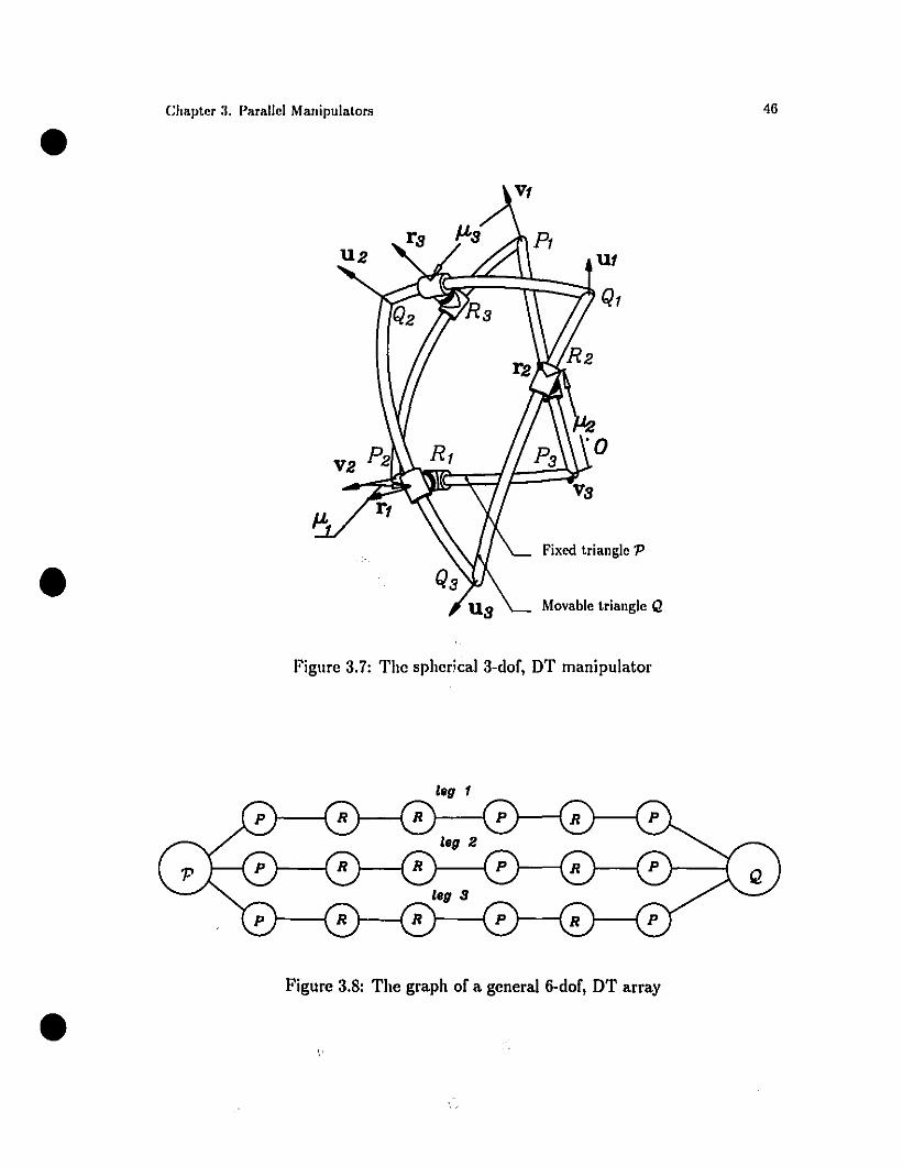
•Chapter :1. l'arallel Manipnlators 46

•

V2

Fixed triangle op

Movable triangle Q

•

Figure 3.7: The spher.ical 3-dof, DT manipulator

189 1

Figure 3.8: The graph of a general 6-dof, DT array

Chebyshev-Grübler-Kutzbach formula for spatialmechanisms (Angeles, 1988), namely,•Chapter 3. Parallel Mallipulators

1= 6(n - 1) - 51'

4ï

(a.2)

•

•

where n and l'are, respectiveiy, the numbers of links and of c!ementftry Il or P pairs.

For this array, we have n = 1ï and Il = 18, and hencc, the dof is

1= 6 x 16 - 5 x 18 = 6

Triangle l' is designated the fixed triangle, while Q is the movable triangle.

Moreover, the previous array is, in fact, the graph of the manipulator depicted in

Fig. 3.9. The manipulator has six degrees of freedom, but only three legs. Then,

the degree of paral1elism dop, based on eq.(1.1), is equal to 0.5, which lI1eans t.hat

we should actuate two jofii'ts pel' leg. If one chooses to actuate t.he first t.wo joints

in each leg, the manipulator is the general DT manipuiator, of which t,he phumr

and spherical DT manipu!ators are special cases. Some alternative designs of t.his

manipulator are given in the subsection below.

3.4.2 Other Versions of Spatial DT Manipulators

As explained in the previous subsection, one can choose alternative sets of actuating

joints for the 6-dof, DT manipulator. One practical alternative would be ta actuate

the first two prismatic joints of each leg, instead of actuating the first two joint,s.

Moreover, we can also have a 3-dof spatial DT manipulator. The structure of this

dc:wice is similar to that of its 6-dof counterpart, except that we omit the intermediate

prismaticjoint of each leg. The graph of such a mdnipulator is depicted in l''ig. a.lO.The interesting feature of this manipulator is that we can make the distance between

the two prismatic joints of each leg a:. smal1 as possible. In this way, we can get l'id

of long legs, which are a major source of structural flexibîlity.

For this manipulator, we have a number of links n = 14 and the number of elc­

mentary joints p = 15. The dof of the manipulator, thus, is obtaincd by substituting

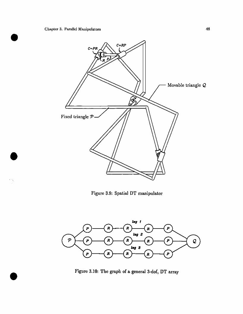
Movable triangle Q

•

•

•

Chapter :1. Parnllel Manipnlators

Figure 3.9: Spatial DT manipulator

Figure 3.10: The graph of a general 3-dor, DT array

48

•

•

•

Chaptcr 3. Parallcl Mal1ipulators

these values into eq.(3.2), namely,

1=6 x 13 - 5 x 15 = 3

Therefore, the degree of parallelism dop, based on eq.( l.l), is equal to one, which

means that one can aduate one joint per leg to move triangle Q. This mot.ion can

be produced by aduat.ing the first prismatic joints of the legs, 50 t.hat all the motors

remain conveniently fixed to the ground.

1""

•

•

•

Chapter 4

Direct Kinematics

4.1 Introduction

'l'he direct kinematics (OK) of the manipulators introduced in Chapter 3 is the

subject of study of this chapter. The OK problem leads to a quadratic equation for

the planar DT manipulator and to a polynomial of 16th degree for the spherical DT

manipulator. Moreover, the OK of ail versions of the spatial DT manipulators are

formulated. For the sake of completeness, the solution of the OK problem for planar

and spherical 3-RRR manipulators are included.

4.2 Planar Manipulators

4.2.1 Planar 3-DOF, 3-RRR Manipulator

The OK problem of the planar 3-RRR manipulator, introduced in Example 3.2.1.1,

is the subject of this subsection. This problem is weil represented in the literature.

Hunt (1983) showed that the problem has at most six real solutions, but he failed to

find the underlying polynomial. Merlet (1989) found a polynomial of degree 12 for

the problem, which is not minimal. Recently, Gasselin and Sefrioui (1991) derived

the minimal 6th-degree polynomial and gave an example having six real solutions.

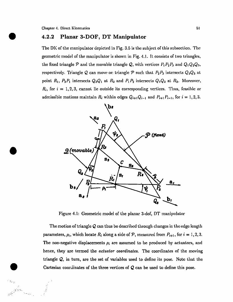
•Chapter 4. Direct Kincmaties

4.2.2 Planar 3-DOF, DT Manipulator

5\

•

•

The DI( of the manipulator depicted in Fig. 3.5 is the subject of this sllbsection. The

geometric mode! of the manipulator is shown in Fig. 4.1. Il. consists of two tl'Ïanglcs,

the fixed triangle 'P and the movable triangle 12, with vertices PI P2/~1 and QI Q2Q:h

respectively. Triangle Q can move or,. triangle 'P snch that 1'21'3 int,ersects Q2Q3 <LI.

point Rh 1'31'. intersects Q3QI at R2 and 1'11'2 intersects Q.Q2 at /l3' Moreover,

/li, for i = 1,2,3, cannot lie outside its corresponding vertices. Thus, feasihle or

admissible motions maintain /li within edges Qi+IQi-1 and Pi+1 Pi- h for i = 1,2,3.

a, ..

Q, ~

Figure 4.1: Geometrie model of the planaI' 3-dof, DT manipulator

The motion of triangle 12 can thus be described through changes in the edge length

parameters, pi, which locate Ri along a side of 'P, measured from Pi+l' for i = 1,2,:J.

The non-negative displacements Pi are assumed to be produced by actuators, and

hence, they are termed the actuator coordinatcs. The coordinates of the moving

triangle 12, in turn, are the set of variables used to deline its pose. Note that the

Cartesian coorJinates of the three vertices of Q can be used to deline this pose.

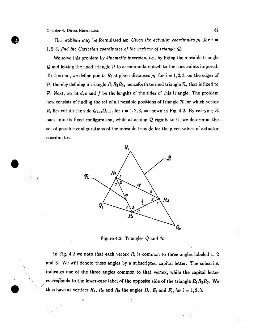
Chnrler 4. Direct I<inemalics 52

•

•

The problem may be formulated as: Civen the aetuator l'oordinates pi, for i =

1,2, :3, fin" the Cartesian l'oordinates of the vertil'es of triangle Q.

We solve this problem by kinematil' inversion, i.e., by fixing the movable triangle

Q and letting the fixed triangle 'P to accommodate itself to the constraints imposed.

'lb this end, we define points R; al. given distances pi, for i =1,2,3, on the edges of

'P, thereby defining a triangle RI R2 Ra, henceforth termed triangle n, that is fixed to

.". Next, we let d, e and f be the lengths of the sides of this triangle. The l'roblem

now consist~ of finding the set of ail possible positions of triangle n for which vertex

Ri lies within the side Qi+IQi-l, for i = 1,2,3, as shown in Fig. 4.2. By carrying nback into its fixed configuration, while attaching Q rigidly to it, we determine the

set of possible configurations of the movable triangle for the given values of actuatol'

coordinates.

Q,

Figure 4.2: Triangles Q and n

111 Fig. 4.2 we Ilote that each vertex R; is common to three angles labeled 1, 2

and 3. We will denote these angles by a subscripted capital letter. The subscript

indicates one of the three angles common to that vertex, while the capital letter

. corresponds to the lower-case label of the opposite side of the triangle Rt R2 Ra. We

thus' have at vertices R.. R2 and Ra the angles Di, Ei and Fi. for i = 1,2,3.

•

•

•

Chapter 4. Direct Kinematics

Considering triangle QI RaR2 , the law of sines for triangles yiclds

wherecl

(lI = -:-~"7sin(Qd

Similarly, for triangle QaR2RI we have

whereJ

(l2 = -:-7::::-"7sin(Qa)

Adding sidewise eq.(4.l) to eq.(4.2) gives

where

b = QIQa

From triangle Q2R I Ra, we have

But

Substitution of Fa from eq.(4.5) into eq.(4.4) yields

5a

(4.'1)

(4.5)

(4.6)

•CIUlplcr 4. Dirccl J<Încrnalics

Again, we have

54

(4.7)

Substitution of D, from eq.(4.6) into eq.(4.7) yields, in turn,

where

(4.8)

Snbstit,uting the expression for sin(D3 ) from eq.(4.8) into eq.(4.3), we obtain

• with bl and b2 defined as

(4.9)

ln eq.(4.!J), wc substitute now the equivalent expressions for cosines and sines

gi ven below:

1 _x2

cos(FJl = 1 2 '+x. (F) 2xsin Il =

1+x2

•

where x is the tangent of one half of the angle FI'

UpOIl simplification, eq.(4.9) leads to

(4.10)

•Chaptcr 4. Direct l\incmatÎcs

with ch C2 and C3 defincd as

Solving eq.(4.1O) fol' x givcs

5;)

The above expression thus leading to thc rcsult bclow:

('1.11)

•

Theorem 1: Given Iwo ldang/es 'R and Q, wc can inscribc 'R in Q i1l lit II/ost

Iwo poses such lhlll vel'lex Ri is /ocaled on lhe edflcs Qi+IQi-1 oJ l.1·Ïll1lfJ/c Q, Jm'i=l,2,3.

Example 4.2.2.1:

Consider the fol1owing sides assigned to thc triangles 'P and Q:

Choose three points, Rh R2 and R3 , located !ly thrcc actuator coordinatcs spccilicd

as PI -= O.? m, P2 = 0.14161 m and P3 = 0.03064 m. Thcsc valucs pl'Oducc the

lengths d, e and J given below:

d = 0.33166 m, e = 0.26458 m, J = 0.2 m

•The two roots of eq.(4.11) are:

XI =1.0788 , X2 =0.4447

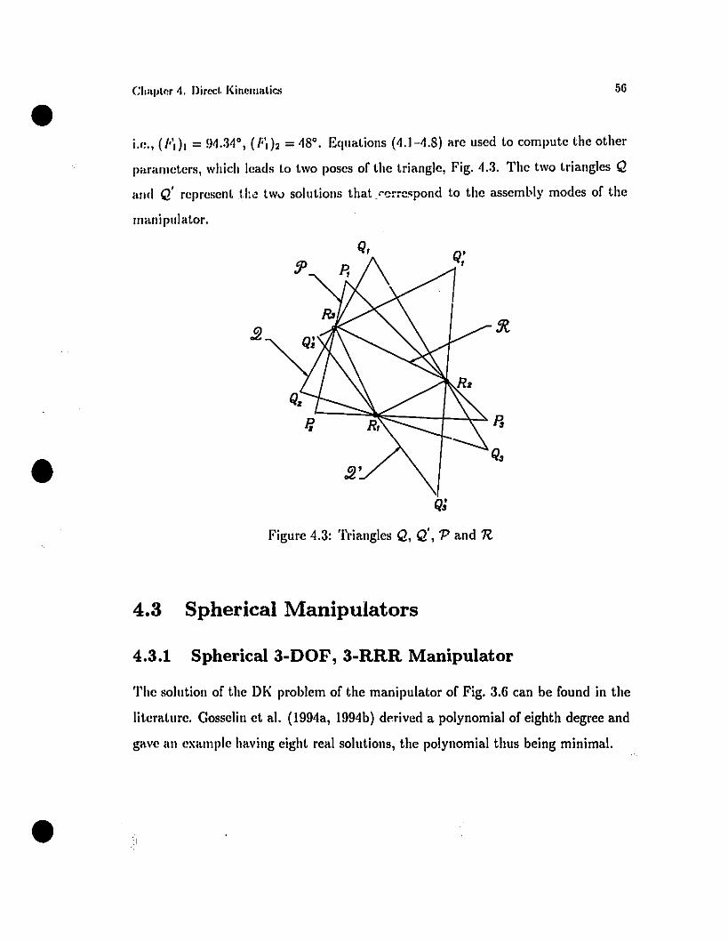
•CI",,,lcr 4. Dirccll<inclIIlllics 56

•

•

Le., (Fdl = !J4.34°, (Fd2 = 48°. Equations (4.1-4.8) are used to compute the other

pararneters, which leads to two poses of the triangle, Fig. 4.3. The two triangles Q

and Q' represent t.h~ twv solutions that r~rrcspond to the assembly modes of the

llJanipulator.

Q;

Figure 4.3: Triangles Q, Q', 'P and n

4.3 Spherical Manipulators

4.3.1 Spherical 3-DOF , 3-RRR Manipulator

The solution of the DI\ problem of the manipulator of Fig. 3.6 can be found in the

litcrature. Gosselin et al. (1994a, 1994b) d"rived a polynomial of eighth degree and

gave an exarnple having eight real solutions, the polynomial thus being minimal.

•Chapter 4, Direct Kincmaties

4.3.2 Spherical 3-DOF, DT Manipulator

5;

•

•- ----'~----

The DI( of the manipulator depicted in Fig, 3,7 is the subjecl of this subsect.ion.

The manipulator consists of two triangles, the fixed triangle P and the 1110mble

triangle Q, with vertices p. P2P3 and QIQ2Q3, respectively. Moreover, the side P21~1

of 'P intersects tl,e arc Q2Q3 of Q at point ni. Wc denote by 112 and n3 the ot.hel'

intersection points, that are defined correspondingly. Moreover ni, for i = 1,2,:1,

cannot lie outside its corresponding vertices. Thus, feasible or nd.ilissible Illotious

maintain ni within edges Qit .Qi-I and Pit. Pi-h for i = 1,2,3,

Thus, the motion of triangle Q can be described through the arc lengths IIi of

Fig. 3.7, or aeiuatOl' cOOl'dinates, for i = 1,2,3. Likewise, the Cart.csiiUl coordinat.es

of the moving triangle Q are the set of variables defining its orient.at.iou. Not.e t.hat

the Cartesian coordinates of the three vertices of Q can be determined once it.s

orientation is given.

Similar to the direct kinematics of the planaI' DT manipulat.or, t.he saille pl'Oblmn,

as pertains to the spherical manipulator, may be formulated as: Givell /.hc acl.1l11/m'

cOOl·dina/.es P.i, fod = 1,2,3, find the CII1'/.csian cOOl'dinates of the vel,tices of tri/lIlgle

Q.

Again, we solve this problem by kinematic invcI'sion, i.e., by fixing the Illovable

triangle Q and letting the fixed triangle P accommodate itsclf t.o the constraint.s

imposed. '1'0 this end, wc define points ni at given arc lengths Jli, for i = 1,2,:1,

on the ed~es of P, thereby defining a triangle n. n2n3 , hcnceforth terl11ed triangle

n, that is fixed to 'P. Next, wc let d, e and f be the sides of this triangle. The

problem now consists of finding the set of ail possible orientations of triangle n for

which vertex ni lies within the side QitlQi-h for i = 1,2,3, as shown in Fig. 4.4.

By carrying n back into its fixed configuration, while attaching Q rigidly to it, wc

determine the set of possible configurations of the movable triangle for the given

values of actuator coordinates.

In Fig. 4.4 we note that each vertex Ri is common to the three spherical angles

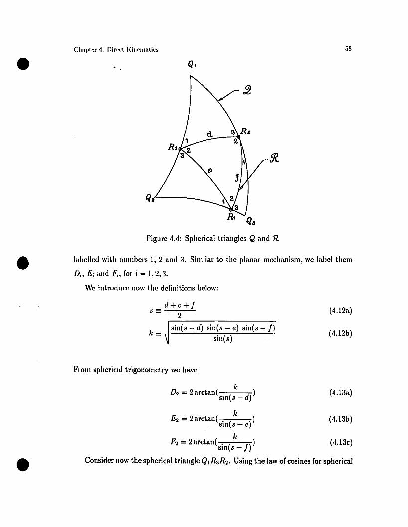
•Chaptf~r '1. Dirf~d I<irwlllatics

Q,

Qa'L---__

:;8

•Figure 4.4: Spherical triangles Q and n

labclled with nnlllbers l, 2 and 3. Simi\ar to the planaI' mechanisll1, we label them

Di, Bi and Fi, fol' i = 1,2,3.

We introdllce now the definitions below:

d+c+Is=• - 2

~..::...._--------

(4.12a)

k=:sin(s - d) sin(s - c) sin(s - Il

sin(s)(4.12b)

Consider now the spherical triangle QI RaR2• Using the law of cosines for spherical•

From spherical trigonometry we have

k

E'-? ( k )2-_ arctan . ( )

5111 S - c

k1"2 =2arctan( . ( I))

Slll s -

(4.13a)

(4.13b)

(4.13c)

Substitution of the expressions for cos Eaand sin Ba from cq.(4.15a) into CCl.(·1.I4a),

we obtain

•

•

Chaptcr 4. Direct Kincmatics

triangles, we have

cos Q: - - co;; F\ cos E3 + sin FI sin E3 cos cl

Similarly, for the spherical triangles Q2 RI/la and QaU2111 wc havc

cos Q2 = - cos DI cos /~ + sin DI sin Fa cos c

cos Qa = - cos El cos Da +sin El sin Da cos J

Bowever,

Fa = 71' - FI - F2

Da = 71' - DI - D2

where

(4.1-la)

('1.1'11»

('1.1 'le)

(4.\.'ia)

(4.151»

('1.I5c)

(4.16a)

ail = cos E2

ala = cos cl cos B2

alfi = - COSQI

SI = sin FI

S2 = sin El

Ul2 = - sin E'l

(l1.1 = cos cl sin E2

CI = cos FI

C2 = cos BI

•Similarly, substitution of eq.(4.15b) into eq.(4.14b) yiclds:

(4.l6h)

•Chnptr.r 4. Direct I<inmnatics 60

wherc

U24 = cos e sin 1'2

C3 = cos DI

I,ikewise, substitution of eq.(4.1.5c) into eq.(4.l4c) yields:

(4.l6c)

•where

ll33 = cos f cos D2 ll34 = cos f sin D2

Equations (4.l6a-c) must be solved simultaneously to determine the values of

angles DI. El and FI, ln the above equations, we substitute now the equivalent

expressions for cosines and sines given below:

2X i

I+x~Si =

1- x~1

ci =l+ ~'X,

•where :ri, for i = 1,2,3, are the tangents of one half of the angles FI. El and DI>

respectively.

Vpon simplification, eqs.(4.16a-c) lead to these trivariate polynomial equations

in :V .. X2 and X3' namely,

•

•

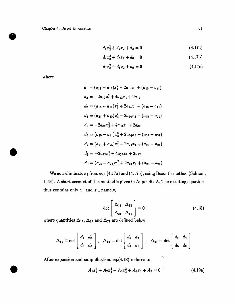
C:1'Jp~~r ~. Dircct I\incmatics

cllX~ + cl2X2 +cla = 0

cl'IX~ +d5X2 +da = 0

d,x~ +dsxa +dg = 0

whcrc

cll = (ail + aI5).1'~ - 2al.IXI + (a15 - ail)

cl2 = -2aI2x~ +"alaXI +2al2

cla = (a15 - all)x~ +2ll l.IXI + (a15 - ail)

d4 = (llal +aa5)X~ - 2lla4Xa + (a:15 - aad

cl5 = -2lla2X~ +"claaxa +2lla2

dG = (lla5 - aadx~ +2lla4Xa + (lla5 - CI:II)

d, = (a21 +ll25)X~ - 2ll24 XI +(ll25 - (121)

ds = - 2ll22X~ +4ll2aX1+21122

61

('l.lia)

(".lib)

(".lie)

Wc now eliminatc X2 from eqs.(4.1ia) and (4.1 ib), using Bczout's IlIcthod (Salmon,

1964). A short account of this method is givcn in Appcndix A. Thc rcsnlting cquat.illn

thus contains only XI and Xa, namely,

[

~II ~12]dct =0~21 ~II

where quanti tics ~II' ~12 and ~21 arc dcfincd bclow:

[dl da] [cl5 d2]~11 == det , ~12 == det ,d4 dG d'I dl

(4.18)

•After expansion and simplification, eq.(4.18) rcduccs to

(4.l9a)

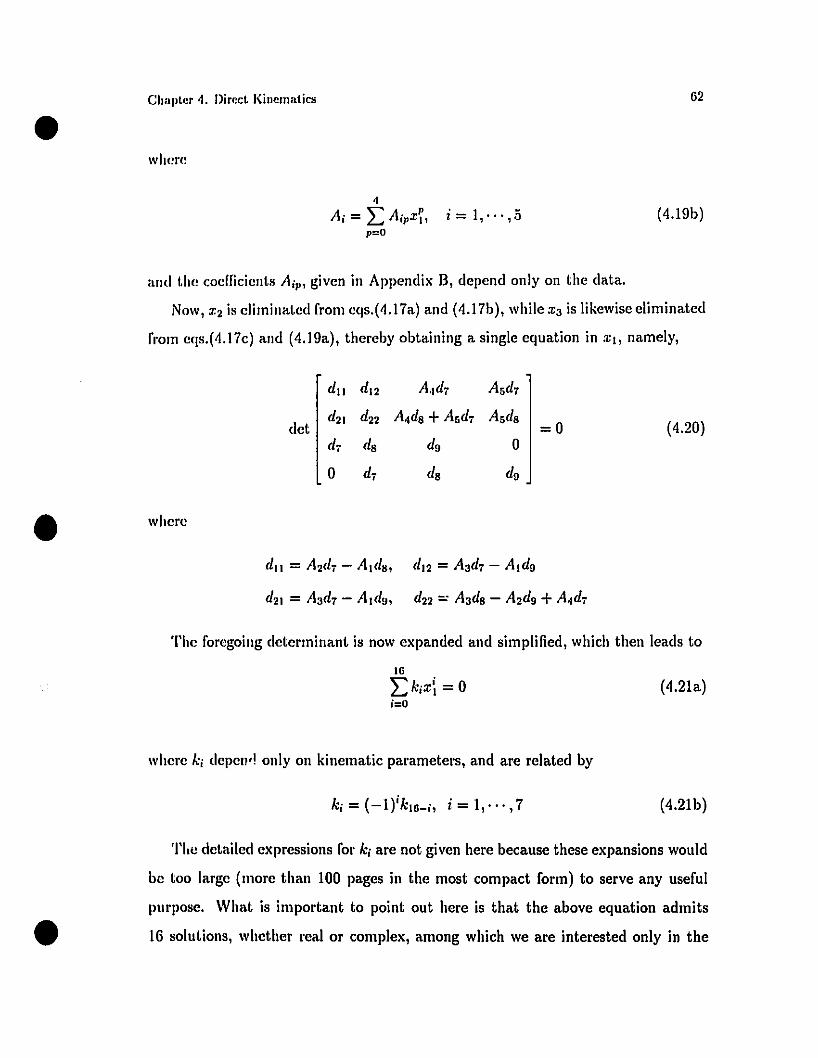
•CI",,,ter ~. Direct J<illematics

where

4

Ai=LAipX~, i=I,···,5p=O

62

(4.19b)

amI the coefficients Aip , given in Appendix B, depend only on the data.

Now, X2 is e1irninated from eqs.(4.17a) and (4.17b), while X3 is likewise elirninated

from eqs.(4.17c) and (4.19a), thereby obtaining a single equation in Xh namely,

• wher"

det

du dl2 A.1d7 Asd7

d21 d22 A.lds +Asd7 Asds

d7 ds dg 0

o (/7 ds dg

=0 (4.20)

du = A2d7 - Alds, dl2 = A3d7 - Aldg

d21 = A3d7 - Aldg, d22 :: A3ds - A2dg+A4d7

'l'he for"going deterrninant is now expanded and simplified, which then leads to

16

LkiX\ = 0Î=O

wher" ki depen<! only on kinematic parameters, and are related by

(4.21a)

(4.21b)

•'l'l,,, detailed expressions for ki are not given here because these expansions would

b" too large (more than 100 pages in the most compact form) to serve any useful

purpose. What is important to point out here is that the above equation admits

16 solutions, whether real or complex, among which we are interested only in the

•

•

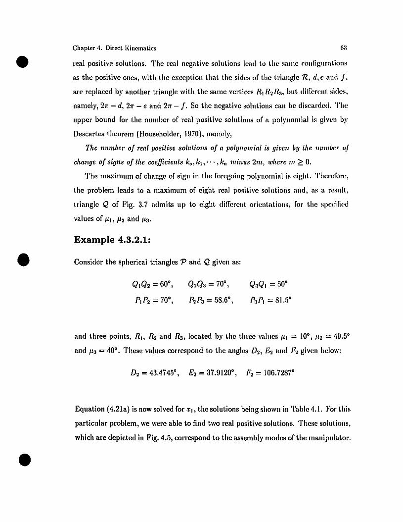
Chapter 4. Direct Kinematics

l'cal positive solutions. The real negative solutions lead t.o the same conlignmt.ions

as the positive ones, \Vith the except.ion t.hat. the sides of t.he I.riangle n, cl, c and f.arc replaced by another triangle \Vith t.he same vert.ices /lI R2 /h, hnl. dHrerent. sides,

namely, 271' - d, 271' - e and 271' - f. So the negative solntions can he discal'<led. The

upper bound fol' the number of real posit.ive solut.ions of a polynomial is giwn by

Descartes theorem (Householder, 1970), namely,

Thc nllmbe/' of "eal positiue sollltions of a polynomial is giuell by the nUII/ba of

change of sign.~ of the coefficients k., kl,"', k" millllS 2m., whc/'c 111 ;:: O.

The maximum of change of sign in the foregoing polynomial is eight.. Thereforc,

the problem leads t.o a maximum of eight real positive solut.ions and, as a. result.,

triangle Q of Fig. 3.7 admits up to eight different orient.at.ions, fol' t.he specilicd

values of 1110 112 and 113.

Example 4.3.2.1:

Consider the spherical triangles l' and Q given as:

QIQ2 = 60·,

PIP2 = 70·,

Q2Q3 = 70·,

P2 P3 = 58.6·,

Q3QI = 50·

P3 PI = 81.5·

•

and three points, Rh R2 and R3 , located by the tl1l'ee values III = 10·, 112 = ~!).5·

and 113 = ~Oo. These values correspond to the angles /J2' B2 and 1'2 given bclow:

/J2 = 43.4ï~5·, B2 =37.9120·, F2 = 106.7287·

Equation (4.21a) is now solved for Xh the solutions being shown in Table ~.l. Fol' this

particular problem, we were able to find two l'cal positive solutions. These solutions,

which are depicted in Fig. 4.5, correspond to the assembly modes of the manipulator.

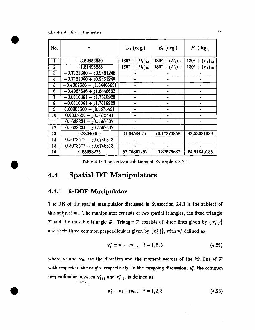
64

FI (deg.)El (deg.)DI (deg.)

Table 4.1: The sixtF.:en solutions of Example 4.3.2.1

Chapler 4. Direct I(inematics

1 -3.52853659 1800 + (Dd13 1800 + (Ed13 1800 + (Fd132 - 1.81493883 1800 + (DdlG 1800 + (Ed16 1800 + (Fl h63 -0.7122360 - JO.9461246 - - -4 -0.7122360 +JO.9461246 - - -5 -0.4987636 - JI.64486621 - - -6 -0.4987636 +JI.6448662 - - -7 -0.0110361 - JI.7618928 - - -8 -0.0110361 +JI.7618928 - - -9 0.00355500 - JO.::m5491 - - -10 0.0035550 +JO.5675491 - - -11 0.1688234 - JO.5567607 - - -12 0.1688234 +JO.5567607 - - -13 0.28340360 31.64584216 76.17273858 42.5302108914 0.5078577 - JO.6746313 - - -15 0.5078577 +JO.6746313 - - -16 0.55098275 57.70801252 99.32576667 64.91849185

•

• 4.4 Spatial DT Manipulators

4.4.1 6-DOF Manipulator

The OK of the spatial manipulator discussed in Subsection 3.4.1 is the subject of

this sul~"cction. The manipulator consists of two spatial triangles, the fixed triangle

'P and the movable triangle Q. Triangle 'P consists of three \ines given by {vi liand their three cornmon perpendiculars given by { ai li, with vi defined as

vi == Vi + tVOi, i = 1,2,3 (4.22)

where Vi and Vo; are the direction and the moment vectors of the ith \ine of 'P

with respect to the origin, respectively. In the foregoing discussion, ai, the common

perpendicular between vi+! and vi_l' is defined as

• ai =ai + tBoit i = 1,2,3 (4.23)

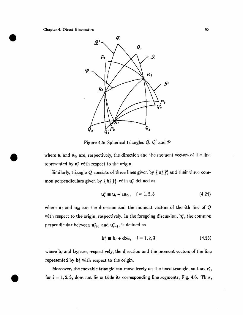
•Chapter 4. Direct I\inematics '"u.l

•Figure 4.5: Spherical triangles Q, Q' and 'P

where ai and aOi are, respective1y, the direction and the moment vedors of the Hne

represented by ai with respect to the origin.

Similarly, triangle Q consists of three Hnes given by {ui nand their three com­

mon perpendiculars given by {bi n, with ui defined as

ui == Ui +CUOi, i = 1,2,3 (4.24)

where Ui and UOi are the direction and the moment vectors of the ith Hne of Q

with respect to the origin, respectivcly. In the foregoing discussion, bi, the common

perpendicular between ui+1 and ui_Il is defined as

bi == bi +cbOi ' i = 1,2,3 (4.25)

•where bi and bOi are, respectively, the direction and the moment vectors of the Hne

represented by bi with respect to the origin.

Moreover1 the movable triangle can move freely on the fixed triangle, 50 that ri,

for i = 1,2,3, does not lie outside its corresponding Hne segments, Fig. 4.6. Thus,

•

•

•

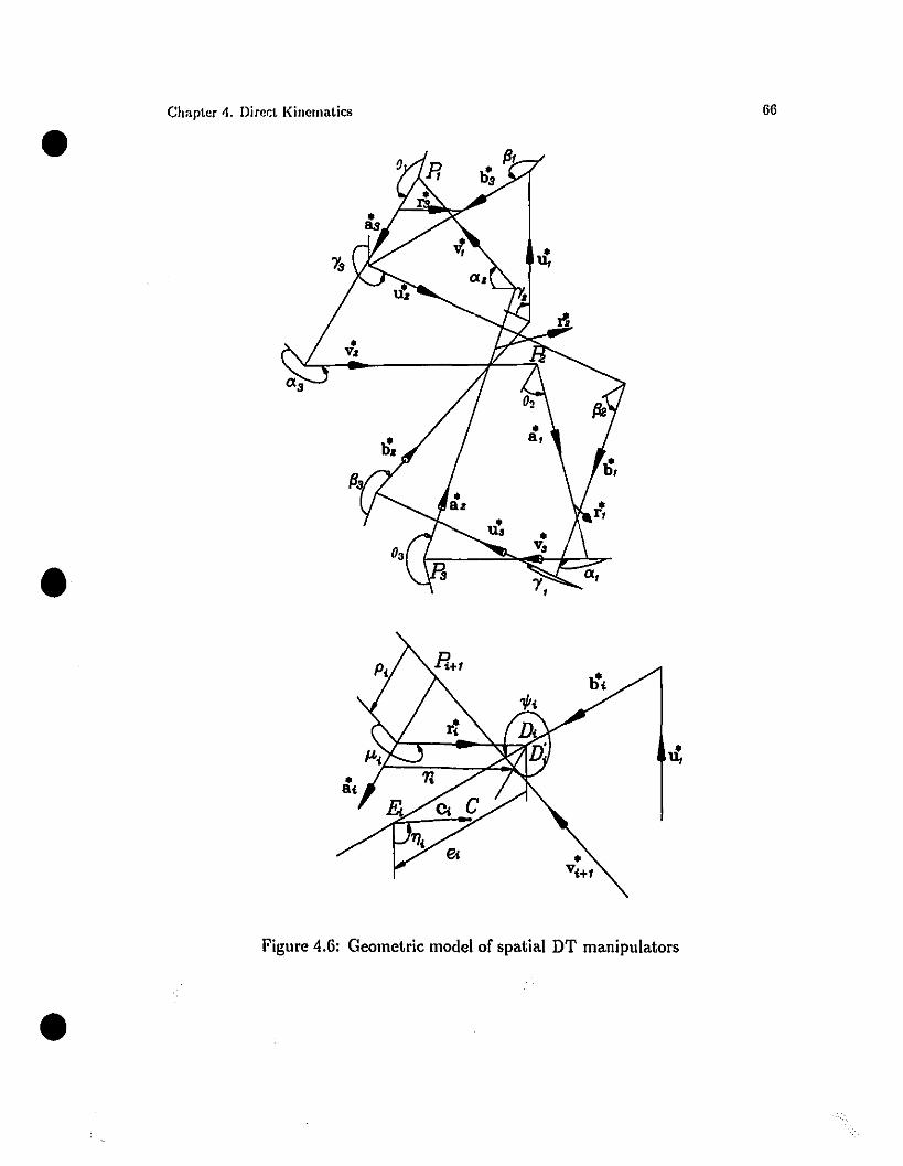
Chapler 4. Direcl Kinernalics

Figure 4.6: Geometrie model of spatial DT manipulators

55

for feasihle or admissible motions, ri must intersect ai and bi wi' ilin their tine­

segments. The motion of triangle 12 can thus be dcscribed throngh changes in the

edge-Iengtl, parameters Pi, which locate ri along a side of 'P, measured from Pith

and changes in the twist angle between vi+1 and ri, IIi, for i = 1,2,3. In other words,

this motion can be described through changes in the dual angles Iii, for i = 1,2,:1.

ln this discussion, ri is the dual representation of a line whose direct.ion and moment

vectors are specified by ri and rOi, respectively, i.e.,

•Chapter 4. Direct Kinematies

ri == ri + crOi, i = 1,2,3

6;

(4.2Ha)

and fti is the dual angle defined as

fti == /Li +CPi, i = 1,2,3 (4.2Hb)

•

•

The changes in fti, for i = 1,2,3, are assumed ta he prodnced byactuators,

and hence, they are termed the actllatm' cool'llinatcs. The three lines {bi nof the

moving triangle, in turn, are the set of variables used ta define its pose. Note that

three !ines can he used ta define a spatial triangle.

The DK problem may he formulated as: Given the actlw{(I7' cOOl'dinates Îli, fm'

i = 1,2,3, find the thl'ee lines of triangle 12, namely, bi, fOI' i = 1,2,3. Thus, given

{fti n, we define a spatial triangle whose three axes are {ri n. The DJ( problem

thus consists of finding aH triangles Q whose three r.ommon perpendiculars, { bi n.intersect these three axes at right angles.

The problem can be formulated in the same way that was formulated for the

spherical DT manipulators, given in eqs.(4.l4a-4.15c), by changing ail the angles to

the corresponding dual angles. Thus, we would have 12 equations in L8 unknowns,

namely, Di, Êi and Fi, for i=1,2,3..Therefore, we need, at least, six extra etluations,

which makes the problem more comp!icated. Bere, an alternative formulation is

given.

Note that ai can be transformed into bi via a screw motion represented by a

•Chapter 4. Direct I<inernatics

unit dual quaternion fi, namely,

b" .""i = ri ai'

wher" fi is dcfined as

i = 1,2,3

68

(4.27a)

ill which 1ÎJi is the dual angle defined as

i = 1,2,3 (4.27b)

1ÎJi == !/Ji +Cl'i, i = 1,2,3 (4.27c)

Moreover, ri is a transformation of vi+l via a screw motion represented by a unit

dual quatel'llion âi, as shown in Fig. 4.6, namely,

with !/Ji and l'i defined, in turn, as the twist angle and the distance between lines ai

and bi, respectively.

Substitution of the value of l~: from eq.(4.27b) into eq.(4.27a), upon simplification,

leads to

•b" J." + " . J. "i = cos Y/iai ri sin Cf/iai, i=1,2,3 (4.28)

where

ri = âivi+l' i = 1,2,3 (4.29a)

." . + " . •ai == cos Ili ai sm Il;, i=1,2,3 (4.29b)

Substitution of the value of ri from eq.(4.29a) into eq.(4.28), upon simplification,

leads to

b" .Î." + .. .Î. " "+. . . .Î. "" "i = cos 't'iai cos Ili sin o/iVi+l ai sin Jli sin Y"iaj Vi+l ai' i=l,2,3 (4.30)

•

Equation (4.30) leads to 18 scalar equations in 24 unkllowns, namely, the three lines

represented by {bi Hand the three dual quantities { 1ÎJi H.MO,m'Ver, we recall the angular c1\>sure e'luation from eq.(2.57), which, for mov­

able tl'ial..,le, leads to

(4.31a)

•Chaptcr 4. Direct Kincmatics

where bi, for i = 1,2,3, are unit dual quaternions, defincd as

ml

-. - b"-bi == cos ,i + i <IIl'i>

in which -ri is the dual angle defined as

i = 1,2,3 (4.:llb)

-ri == ,i +Cbi, i = 1,2, 3 (4.:llc)

where ,i and bi are the twist angle and the distance bctwccn lincs U;+I and ui_l'

respectively. Moreover, pre-multiplying both sides of cq.(4.:lla) by k(b;), lcads 1.0

bj bj = k(bi) (4.32)

•

Equation (4.32) thus leads to eight extra equal.ions to givc a total of 26 cqmüions

in 24 unknowns, whose roots are the solutions of thc DI< problem al. hand.

Moreover, substituting the values of bj, b; and b; from eq.(4.3Ib) inl.o cq.(4.:l2),

upon simplification, leads ta

cos -rI cos -ra +bj cos -rI sin -ra +bj sin -rI cos -ra +(4.:1:1)

Finally, substituting the values ofbi, for i = 1,2,3, from cq.(4.30) int.o cq.(4.:I:I),

leads to eight equations in six unknowns, namely, six parametcrs in thrce dual quan­

tities ~i' for i = 1,2,3. Among the eight equations, only six are indcpendcnt, and

the problem should admit sorne solutions.

Example 4.4.1.1:

The fixed triangle is given by three dual vectors vi, for i = 1,2,3, via their dircction

and moment vectors, as explained in eq.(4.22), Le.,

•T ['/'VI = [1, 0, 0], V 10 = 0, 0, 0]

T TV2 = [0,0,1], V20 = [1,0,0,]

T TVa = [0, -1,0], Vao = [1,0,1]

(4.34 )

The diredion and moment vectors of the tliree common perpendiculars to the fore-•Chaptcr '1. Direct KinclIlatics

going given lines, {ai H, arc

al = [-I,O,O]T,

a2 = [o,o,-If,

a3 = [0, l ,of,

alO = [0, -l, I]T

a20 = [0, -l, OlT

Ta30 = [0,0,0]

iO

(4.35)

•

Moreover, the moving triangle :.. given by its three sides, namcly,

1'1 = 1.99133 +&37268

1'2 = 0.876816 +cO.737494

1'3 = 1.74.577 +cO.123211

I~inally, six aduator coordinates are given in dual form as

ÎJ.I = -71" + cO.5

ÎJ.2 = -2.15873528 +cO.75

,Î3 = -371"/4 + cO.25

(4.36)

(4 ,,~\.v. J

Snbstitution of the foregoing data into eq.(4.33), upon simplification, \eads to

q=O (4.38)

•

where q is ~,n 8-dimensional vedor with only six independent components. The eight

components of q are given in Appendix C.

So\ving eq.(4.38) for l'i and .,pi, for i = 1,2,3, leads to the six real solutions in

Table 4.2.

Substitution of the data from eqs.(4.34 - 4.37) and the foregoing values for ri and

if';, for i = 1,2,3, into eq.(4.30), gives bi, for i = 1,2,3. For example, for solution

No. 4, one may obtain three Iines of the moving triangle as

bi = [-0.894427, -0,447214,OjT +([0.223608, -0.447214, 1.11803jT

bi = [0.5547, -0.83205, ojT +([0.208013,0.138676, 0,416026jT

bi = [0.707107,0, 0.707107f +c[0.176777, 0.353553, -0.176777f

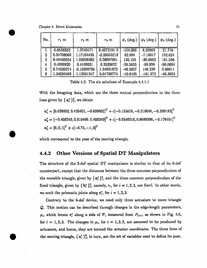
No. r. m r2 m 1'3 m !/JI (deg.) !/J2 (deg.) !/J3 (deg.)

1 0.0558852 1.0740471 0.4072191 6 -154.806 8.32983 21.7462 0.34708068 1.17104435 -0.20553218 62.084 -7.16017 152.62,13 0.46406054 1.03938365 0.28097901 135.155 -39.8682 101.5564 0.4999920 0.4160031 0.3535622 -26.5655 -89.999 -90.00045 0.74620074 -0.10399796 1.54681873 -46.5857 146.239 9.860116 1.34650493 1.13581347 0.01708774 -10.8435 -161.372 -46.3(i52

• Ch~pter 4. Direct Kinematics

Table 4.2: The six solutions of Example 4.4.1.1

i\

•

•

With the foregoing data, which are the three mutual perpendiculars to the t,hl'ce

lines given by {ui }~, we obtain

ui = [0.639602,0.426401, -0.639602f + ([-0.193819, -0.218046, -0.339l83f

ui = [-0.408249,0.816496. O.408249f + ([-0.0340218,0.0680398, -0.170101 fi'u; = [0,0, W+ ([-0.75, -l,of

which correspond to the pose of the moving triangle.

4.4.2 Other Versions of Spatial DT Manipulators

The structure of the 3-dof spatial DT manipulator is similar to that of its 6·dof

counterpart, except that the distances between the three common perpcndicnlal's of

the movable triangle, given by {ai n, and the threc common perpendiculars of the

fixed triangle, given by {bi n, namely, ri, for i = 1,2,3, are Iixe~l. In otller words,

we omit the prismatic joints along ri, for i = 1,2,3.

Contrary to the 6-dof device, we need only three actuators to mave triangle

Q. This motion càn be described thl'ough changes in the edge-Iength parametcr's,

pi, which 10cate ri along a side of 'P, measured from PHil as shown in Fig. 4.6,

for i = 1,2,3. The changes in pi, for i = 1,2,3, arc assumed to be produced by

actuators, and hence, they are termed the actuator coordinatcs. The three lines of

the moving triangle, { ui n, in turn, are the set of variables used to define its pose...

The direct kinematic problem of the manipulator described above is the subject of

this subsection. This problem may be formulated, similarly, as: Given the ar.iltator

coor(lintlte.~ (Ji, fOI' i = 1,2,3, fintl the three lines of triangle Q, namely, bi, for

i = 1,2,3. In order to solve this problem, wc define three ci l'des in planes of normals

{ai n, their radii bcing given by ri, for given value of Pi, for i = 1,:',3. The DI<

problem thus consists of finding ail triangles Q whose three common perpendiculars,

bi, for i = 1,2,3, intersect these three drdes and are perpendicular to ri.

The governing equations are the same as describeJ in eq.(4.33), in which we have

cight cquations in six unknowns. However, ri, for i = 1,2,3, are given and our six

unknowns arc the six angles /li and tPi, for i = 1,2,3. Again, among these eight

equations, only six are independent, and the l'roblem should admit sorne solutions.

•Chapter 1. Direct I<inematics 72

•Example 4.4.2.1:

Given arc the same fixed and movable triangles as in Example 4.4.1.1., and three

lengths ri, for i = 1,2,3, as

l') = 0.5, 1'2 = 0.416024, ra = 0.353553

Moreover, the three actuator coordinates are given as

PI = 0.5, P2 = 0.75. Pa = 0.25

(4.39)

(4.40)

Substitution of the foregoing data and the data from eqs.(4.34-4.36) intoeq.(4.33),

IIpon simplification, leads to

q=O (4.41)

•

wherc q is an 8·dimensional vector with only six independent components. The eight

components of q are given in Appendix D.

Solving eq.(4.41) for /li and tPi, for i = 1,2,3, leads ta 26 sets of solutions, as

given in Table 4.3.

Substitution of the data from eqs.(4.34-4.36) and the foregoing values for /li and

,pi, for i = 1,2,3,;nt~ eq~(4.30), gives {bi n. For example, for solution No. 1, we

•

•

•

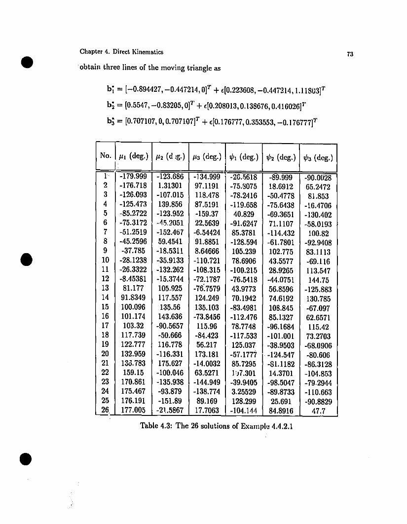
Chapter 4. Direct Kinematies

obtain three lines of the moving triangle as

b; = [-0.894427, -0.447214, W+![0.223608, -0.447214, 1.118U3f

bi = [0.5547, -0.83205, 0]1' +![0.208013, 0.138676, 0.416026]7'

bj = [0.707107,0, 0.707107f +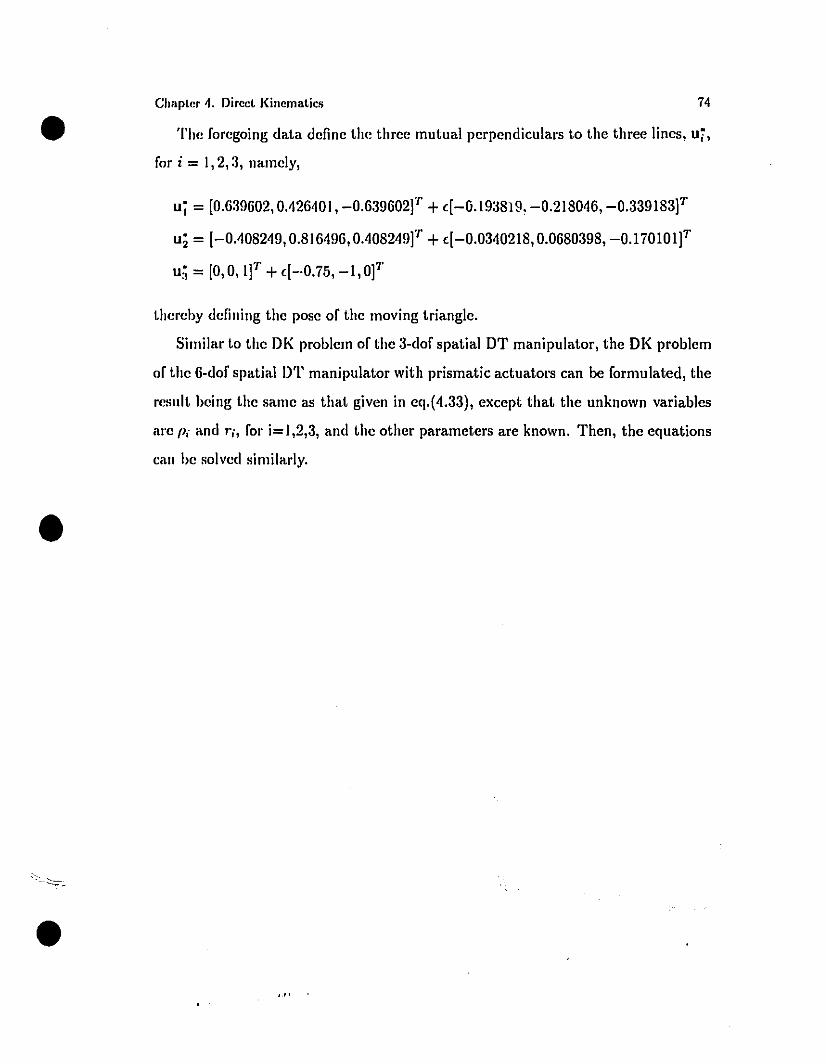![0.176777, 0.353553, -0.176777f

No. 1 III (deg.) 112 (d :g.) lia (deg.) !/JI (deg.) V'2 (dcg.) !/Ja (<lcg.)

1 -179.999 -123.686 -134.999 ' -26.!i618 -89.999 -90.00282 -176.718 1.31301 97.1191 -75.8075 18.6912 65.24723 -126.093 -107.015 118.478 -78.2416 -50.4778 81.8534 -125.473 139.856 87.5191 -119.658 -75.6438 -16.47065 -85.2722 -123.952 -159.37 40.829 -69.3651 -130.4026 -75.3172 -~.5. 2051 22.5639 -91.6247 71.1107 -58.01937 -51.2519 -152.467 -6.54424 85.3781 -114.432 100.828 -45.2596 59.4541 91.8851 -128.594 -61.7801 -92.94089 -37.785 -18.5311 8.64666 105.239 102.775 83.111310 -28.1238 -35.9133 -110.721 78.6906 43.5577 -69.11611 -26.3322 -132.262 -108.315 -100.215 28.9265 113.54712 -8.45381 -15.3744 -72.1787 -76.5418 -44.0751 144.7513 81.177 105.925 -76)579 43.9773 56.8596 -125.88314 91.8349 117.557 124.249 70.1942 74.6192 130.78515 100.096 135.56 135.103 -83.4981 108.845 -67.09716 101.174 143.636 -73.8456 -112.476 85.1327 62.657117 103.32 -90.5657 115.96 78.7748 -96.1684 115.4218 117.739 -50.666 -84.423 -117.533 -101.001 73.270319 122.777 116.778 56.217 125.037 -38.9503 -68.090620 132.959 -116.331 173.181 -57.1777 -124.547 -80.60621 130.783 175.627 -14.0032 85.7295 -BI. 1182 -86.312822 159.15 -100.046 63.5271 1')7.301 14.3701 -104.85323 170.861 -135.938 -144.949 -39.9405 -98.5047 -79.294424 175.467 -93.879 -138.774 3.25529 -89.8733 -110.66325 176.191 -151.89 89.169 128.299 25.691 -90.882926. 177.005 -21..5867 17.7063 -104.144 84.8916 47.7

Table 4.3: The 26 solutions of Exarnple 4.4.2.1

73

The foregoing data define the three mutual perpendiculars to the three lines, ui,

for i = 1,2,3, namcly,•Chapler 4. Direel Kinematies

uj = [0.639602,0.426401, -0.639602jT +c[-u.193819, -0.218046, -0.339183jT

u; = [-00408249,0.816496, 00408249jT +c[-0.0340218,0.0680398, -0.170101rr• T Tua =[0,0, L] +c[-·0.75, -l, OJ

74

•

•

thereby defining the pose of the moving triangle.

Similar to the DK problem of the 3-dof spatial DT manipulator, the DK problem

of the 6-dof spatial DT manipulator with prismatic actuators can be formu lated, the

resnlt being the same as that given in eq.(4.33), except that the unknown variables

are {Ji and '';, fol' i=1,2,3, and the other parameters are known. Then, the equations

can be solved similarly.

..,' '

•

•

Chapter 5

Singularity Analysis

5.1 Introduction

The .Jacobian matrices of several manipuiators, introduccd in Chaptcl' :1, arc derivcd

here in an invariant form. A classification of singularities in pamllcl manipu!ators

into three groups, which is based on the characteristics of thcir .Jacobian matrices,

is proposed and the singularities are identified for thesc manipuiators. Dcriving thc

Jacobian matrices in an invariant form allows us to detect ail singula.-it,ics wit,hin t.hc

manipulator workspaces.

5.2 Jacobian Matrices /,

The dilferential kinematic relations pert.aining to parallel manipulators take on t.hc

form

Jil+Kt = 0 (5.1a)

•

where J and K are the two .Jacobian matrices of the manipulator at hand. Morcover,

il is the vector of joint rates and t is the twist a7'1'ay, which assumes differcnt forllls,

depending on the nature of the task space, namcly,

(5.1 b)

5.2.1 Planar Manipulators of Class A

where the nrst fonn corresponds to planarj the second to sphericalj and the third to

spatial tasks. Moreover, in the foregoing forms, w is the scalar angular vclocity of

the llloving platform and c is the two-dilllensional vclocity vedor of the operatioll

poillt C of the llloving platform for the planaI' case. Likewise, for spherical and

spatial tasks, w denotes the three-dilllensional angular-vclocity vedor of the moving

platforrn. l''inally, for 6-dof positioning and orienting tasks, c denotes the three­

dirnensional velocity of the operation point of the moving body. Therefore, t is a

threc-dirnensional array for planaI' and spherical tasks, while it is six-dimensional for

spatial tasks. So, the .1 acobian matrices arc of 3 x 3 for the planaI' and spherical

devices. For six-dof spatial rnanipulators both J and K arc 6 x 6 matrices.

Bclow wc derive expressions for J and K for the manipulators introduced in Chap­

ter 3. These arc the two general classes of planaI' parallel manipulators, spherical

a-RRR and DT lllaniplllators, and spatial 6-dof, DT manipulators.

•

•

Chllpt"r 5. Singnlllrity Anlllysis ;6

Here, the .Iacobian rnatrices of the 20 different c1ass-A rnanipulators, discussed in

SlIbsection 3.2.1, arc derived. 'l'I.e rnaniplliator, in general form, is depicted in

Fig. :1.2.

The vclocity ccan be written for the ith leg as

(5.2)

whcre ai and qi arc the vedor direded from Pi to Ai and from Ai to Qi, respectively.

Moreover, we have

ai = OiAiai' i = 1,2,3

where Oi is the rate of the ith actuator and Ai is defined as

(5.3a)

•A.= { E,

1 - (1/lIa;l1)1,

if the first joint is revolute

if the first joint is prismatic(5.3b)

in which 1 is the 2 x 2 identity matrix and E is t.he 2 x 2 orthogonal matri x rotating

vectors in a plane through an angle of 90· counterc1ockwise, i. e.,•Chaptcr 5. Singularity Analysis ii

1vI0reover, we have

(5Aa)

where 1i is the rate of the second joint, ri is the veetor direeted from Ai 1.0 qi and

Bi and Ci are defined as

if the first joint is revolute

if the first joint is prismatic

with 0 denoting the 2 x 2 zero matrix. Furthel'lllOre, ë - CIi is given ,L~•

E,

(1/llrdIl1,

if the second joint is revolut.e

if the second joint is prismatic(5Ah)

(5Ac)

ë - CIi =WESi, i = 1,2,3 (5.5)

with veetor Si direeted from Qi 1.0 C, as shown in I~ig. 3.2.

Substitution of the values of Ïli,CIi - Ïli and ë - CIi from eqs.(5.3a), (5Aa) and

(5.5) into eq.(5.2), and simplification of the expression thus resulting leads 1.0

(5.Ci )

where 7i, being associated with an unaetuated joint, should be c1imirmt.ed. '1'0 t.his

end, we define Ei as

• T 'r 7'Oiri Ei(Aiai +Ciri) +wri EiEsi - ri Eië = 0, i = 1,2,3

Upon multiplication of the two sides of eq.(5.6) by rTEi, we obtain

•Ei == { 1,

E,

if the second joint is revolute

if the second joint is prismatic(5.7)

(5.8)

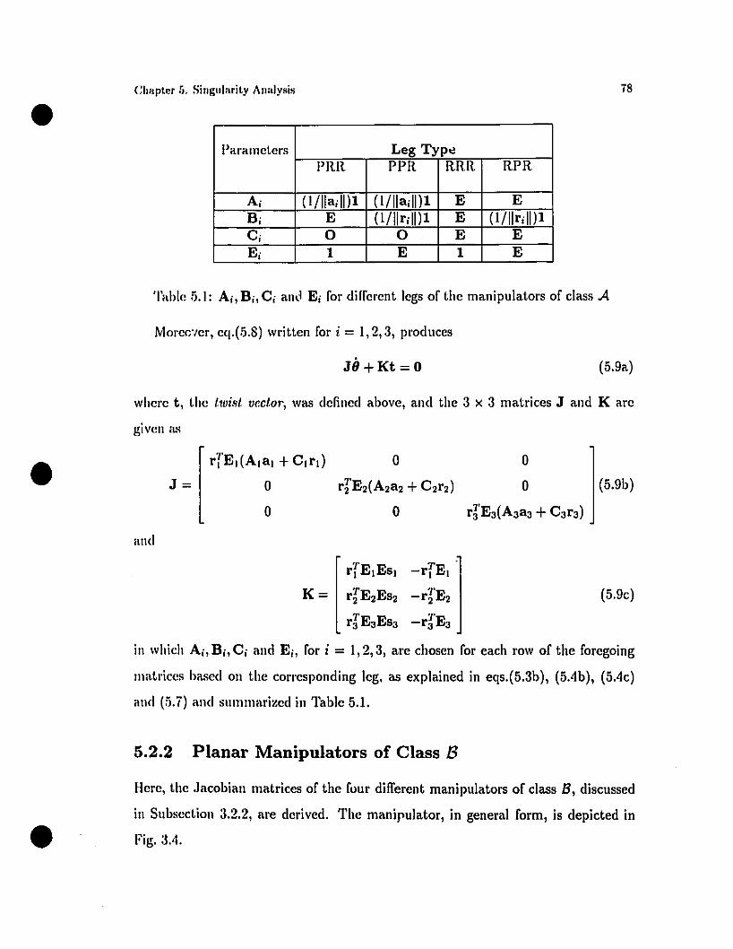
•Chapter 5, Singularity Analysis

l'arameters Leg Typt!l'RR PPR RRR RPR

Ai (I/lladlll (l/lIadlll E EBi E (I/llrdlll E (l/lIrdlllCi 0 0 E EEi 1 E 1 E

Table 5.1: Ai,Bi,Ci an(1 Ei for different legs of the manipulators of dass.A

Morec:,er, eq,(,5.S) written for i = 1,2,3, produces

;8

J8+Kt =0 (5,9a)

where t, the twist uectQl', was defined above, and the 3 x 3 matrices J and K are

•givcn as

rfEI(Alal +C1rd 0

J = 0 rrE2(A2a2 +C2r2)

oo (5.9b)

and

o o

•

7' -rTEIrI E1ES1

K= T -rIE2 (5,9c)r2E2Es27' 7'r3 E3Es3 -r3 E3

in which Ai, Bi, Ci and Ei, for i = 1,2,3, are chosen for each row of the foregoing

1lI1ltl'ices based on the corresponding leg. as explained in eqs.(S.3b), (S.4b), (5.4c)

and (S.i) and sllmnmrized in Table 5.1.

5.2.2 Planar Manipulators of Class B

Berc, the .Jacobian matrices of the four different maniplliators of dass 8, disclIssed

in SlIhscction 3.2,2, arc dcrived. Thc manipulator, in general form, is depicted in

Fig. 3.'1.

•Chapter 5. Singularit)' Anal)'sis

The veloeity C ean he now writtcn for thc ith lcg as

C=V,Ii+(V/li-VAi)+(C-V/li), i= 1,2,3

Moreover, wc have

V,li = OiEiai, i = 1,2,3

iH

(5.10)

(5.11 a)

where ai is the unit veetol' directed from Pi 1.0 Ai and Oi is t.he l'lIt.e of t.he it.h admüor,

while E i is defined as

in which Pi = PiAi.

Furtherlllore, wc have

PiE,

1,

if thc first joint is rcvo\nl,e

if t.he fil'st joint. is prisnmt.ic(5.\ 1h)

•Viii - VAi = wEri, 1. = 1,2,:1

where ri is the veetor dirceted from Ai to Ri. Finally, C - VIIi is givcn ;L~

C- Vn; = ~ibi + WESi, i = 1,2,:1

(5.12)

(5.1:1)

with ~i denoting the rate of the third joint. A unit vect.or b i represents t.he dircct.ion

of the thil'C! joint, which is prismatic, and Si is vcetor dircetcd from ni t.o C, as shown

in Fig. 3.4.

Substitution of t.he values of VAi, Vn; - VAi and C- VI/i from cqs.(5.lla), (5.12)

and (5.13) into eq.(5.1O), and simplification of the expression thns resnlting lcads 1,0

OiEiai + ~ibi + wE(ri + Si) - i: = 0, i = 1,2,:l (5.1~)

where ~i is associated with an unaetuated joint and shon\d be diminat.cd. Mnlt.ipli­

cation of the above equation by bl'E accomplishes this, namc1y,

•Oibl'EEiai - wb7'(ri + Si) - bl'Ec = 0, i = 1,2,:1

Upon writing eq.(5.15) for i = 1,2,3, wc obtain

JB+Kt =0

(5.l.5)

(.5.l6a)

•Chaptcr 5. Singlliarit,y Analysis

\l'1H'rc matrices J and K are given as

80

and

J=

o oo (1i.16b)

K=

l'-b l (rI +sr)

T-b2(r2 +S2)

l'-b3 (r" + s:J) -bIE

(1i.16c)

A :l-RRR spherical parallcl manipuhüor is depictecl in Fig. :1.6. Ali the joints of this

manip"lator arc l'l'volutes and the thre'e motors PI, 1'2 and !':l arc fixed ta the base.

The angnlar vdocity w of the EE can be \l'ritten as

•

5.2.3 Spherical 3-RRR Manipulator

0;1I; +o;v; + :";w; = w, i = 1.2.:3 (ii.li)

\l'hNe li;, V; and W; H1'(' the unit "cet ors painting from the t'enter of the sphere ta

points l';, :1; and Q;. respecti"c1y. :\Ioreover. 0;, 0; and :.,; arc the rates of the joint

attac!led 1.0 the base, tlll' inlermecliatejoint and the joint attached la EE. respeclivcly.

Ilelo\l' wc eiiminate the rates of the unactlwted joints by dot-mlliliplying bath sides

of lhe foregoing eqllation by V; x W;. thereby obtaining

•

Oill;' (Vi X w;) = w· (V; X w;). i = 1.2.:1

which can be \l'ritten in llll'll as

. l'Oi(V; X li;)' W; + (v; x w;) w = 0, i = 1.2.:1

The above eqllations, for i = 1,2,3, are now assembled in the f0I'111

JB +Kw =0

(5.18)

(5.19)

(5.20a)

•Chapter 5. Singularity Analysis

where the 3 x 3 matrices J and K are defined as

al 0 0

J == 0 a2 0

o 0 aa

and

(VI X WljT

K == (V2 X W2jT

(va X wajT

in which

81

(S.20b)

(S.20c)

(.5.21)

•5.2.4 Spherical DT Manipulator

The Jacobian matrices of a spherical paraUel manipulator, as depieted in Fig. 3.7,

are derived here. Let us intl'Oduce the normalized vectors ai and b i , for i = 1,2,:J,

which are perpendicular to the planes of arcs PHI Pi+2 and Qi+1 Qi+2, respeetivc1y,

as shown in Fig. S.1.

Thus,Vi+1 X Vi+2 b. _ Ui+1 X Ui+2

ai=IIvi+1 x Vi+2l1' • - lIui+1 x uidl

where Ui and Vi are both unit vectors directed from 0 to Qi and Pi, respectively.

The angular velocity "" of the EE can now be written as

(S.22)

•

where l'i is the upit vector direeted from the center of the sphere to Ri. Moreover,

ai is the angle between planes of Pi+h Pi+2 and Qi+h Qi+2' while "Yi is the angle

between UH1 and l'i.

The inner procluct of both sicles of eq.(S.22) with l'i x bi, upon simplification,

leacls to an equation free of unactuatecl joint l'ates, namely,

(S.23)

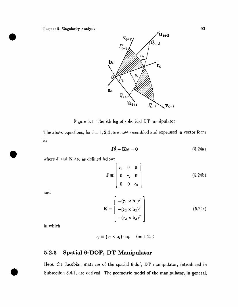
•Chaptcr 5. Singlliarity Analysis 82

Figure .5.1: Thc ith leg of spherieal DT manipulator

Tlw abol'c cqnations, for i = 1,2, :1, are now asscmbled and expressed in l'cetol' form

•as

J8+Kw = 0

whcl"(~ J and K arc as defiued bclow:

CI 0 0

J == 0 C2 0

o 0 C:l

am!

iu which

Ci == (ri x bd, ai, i = 1,2,3

(.5.24a)

(5.24b)

•5.2.5 Spatial 6-DOF, DT Manipulator

Here, the Jaeobian matrices of the spatial 6-dof, DT manipulator, introdueed in

Subseetion 3.4.1, are derived. The geometric model of the manipulator, in general,

is depieted in Fig. 4.6.

The angnlar vciocity w of the moving triangle can be written, for the ith leg, as•Chapter 5. Sillgularity Allalysis 83

/1iai + tPiri + 'iibi = w, i = 1,2,3

Below wc eliminale the rates of the lInactllated joints by dot-mllitiplying both sides

of the foregoing eqllation by bi x ri, thereby obtaining

- ,iiai . (bi x 1',) + w . (bi x l';) = 0, i = 1,2,3 (5.26)

l"loreover, the velocity ë of the operation point of the EE can be written, for the

ith leg, as shown in Fig. 4.6, namely,

•where di and d'i arc the position veetors of Di and D:, in which Di is rixed 1,0 the

line ri while D: is attached to the prismatic joint along that line; so, for i = 1,2,:l

wc have

di = Piai + ,iil'i(ai x l';)

(5.2ïb)

ë-d'i = éibi+W x (eibi+c;)

where Ci is a veetor whose end-point is the operation point and is nOl'lnal 1,0 lin" bi,

and Ci = DiEi.

SlIbstitllting di, d'i - di and ë - d'i fl'Om eq.(5.2ïb) into eq.(5.2ïa), lIpon simpli­

fication, leads 1,0

where i'i and éi , the velocity of the lInaetllated joints, shollid be eliminated, This

can be donc by post-mllitiplying both sides of eq.(5,28) by (bi x ri), i.e.,

•

é = Piai + ,ii7'i(ai x ri) + 7\ri + éibi + CiW x bi + W x Ci, i = 1,2,3

cT(bi x ri) =/>;aT(bi x ri) + /1i7'i(ai x r;)'r(bi x ri) + Ci(W X bif

(bi x ri) + (w x cif(bi x l';) = 0, i = 1,2,3

(!i.28)

(5.29)

•Chapt.cr 5, Singularit.y Analysis

Dividing the foregoing eqllation by /";, lIpon simplification, leads to

84

-ëT(b; x r;)/I'i + p;af(b; x r;J/"; + (I;(ai x rd'I'(bi x r;)+

'1'W (-c;r; +Ci x (b; x r;J)/r; = O. i = 1,2,:1 (,5.:30)

Writing eqs.(.5.26) and (5.30) for i = 1,2.:1. we obtain

JO + Kt = 0 (.5.:31 a)

where t is the twist or Cartesian-vclocity vector, and 0 is the joint-vclocity vector,

defined bclow as

_ '1"'1' '1't = [w , C )

o== [ri" P2, i''', (l,. (12' (l"fI'

Moreover, the fi X fi .Jacobian matrices J and Kan' gi\'en as

(5.:11b)

• J==

K==

0 0 0 -aTI11 ,

0 0 0 0

0 0 0 0'1' 0 0al 1111/1'1 1'1

0 T 0 08 2 111 2/1'2

0 0 '1' / 0a:J 11)-, 1':,

111'1' 0'1'1

111'1' 0'1'2

'1' 0'1'111"T -mf/riq,

'1' '1'q2 -1112/1'2

'1' '1'q" -l11a / ra

0 0

'1' 0-a21112

0 '1'-aa l11a

0 0

1'2 0

0 l'a

(.5.31c)

(5.31d)

•in whicb 111;, l'; ami qi, fOl' i = 1.2, :1, arc dcfined as

111; == b; x r;

'1'l'i == (ai x r;} 111;

q; == (-Ciri +Ci x l11i)/";

(5.31e)

•

•

Chaptcr 5. Singlllarity Analysis

One may write eq.(5.31a) in dual form as

where

aiml+(!J1 0 0

j== 0 T 0a2m2 + (]l2

0 0 aIm3+ (]l3

T + T-ml r.ql

K== -mf + (qiT T-m3 + (ql

w== W + (C/"i

in which

• 1 • • //li == 11i +Pi "i

85

(5.32a)

(5.32b)

(5.32c)

(5.:J2d)

(5.:l2e)

(5.:32f)

Equations (5.32a-c) reducc to velocity relationships of the spherical DT ma­

nipulator as expressed in eqs.(5.24a-c) by omitting the dual parts of the foregoing

equations.

5.3 Classification of Singularities

In parallel manipulators, singularities occur whenever J, K, or both become singu­

laI'. Thus, for these manipulators, a distinction can be made among three types of

singularities, which have different kinemat.ic interpretations, namciy,

1) The first type of singularity occurs when J becomes singular but K is invertible,

i. e., when

• det(J) =0 and det(K) # 0 (5.33)

This type of singularity consists of the set of points where al. least two branches of

the inverse kinematic problem meet. Since the nullity of J is not ~ero, wc can find a

set. of non-~ero actuator velocity veciors iJ for which the Cartcsian vclocity vecior t

is ~ero. Then, non~ero Cartesian vclocity veetors Kt, those Iying in the nullspace of

JT, cannat be prod uced, the manipulator thus losing one or more degrees of freedom.

2) The second type of singularity, occurring only in dosed kinematic dJains, arises

when K becomes singular but J is inverti bic, i. e., when

•Chapl.cr 5. Singularity Analysis

dct.(J) # 0 and det(K) = 0

8(j

(.5.:31)

•

•

This type of singularity consists of a point or a set of points whereby different

branches of the direct. kinematic problem meet. Since the nullity of K is not ~cro. wc

can find a set of non~ero Cartesian vclocity vectors t for 'which the aciuator vclocity

vecior iJ is zero. Then, the mechanism gains one or more nncontrollable degrees of

freedom or, equivalently, cannot resist forces or moments in one or more direciions,

even if ail the act.nators arc locked.

:1) The thinl type of singularity occurs when both J and K arc simultaneously

singnlar, while none of the raws of K wlllishes. Under a singularity of this type,

confignrations arise for which link Q of thl' lIIanipulator can undergo finite motions

('ven if the aduators are locked or. equivalently. it cannot resist forces or moments in

one or more directions over a finite pOl·tion of the workspace. even if ail the aciuators

arc locked. As weil, a finite 1II0tion of the ad ua tors produces no lIIotion of Q and

some of the Cartesian velocity vectors cannot be produced. This type of singularity,

as shown here, is not necessarily architeeture-dependent, contrary 1.0 earlier daims

(Gosselin, 1988; Gasselin and Angeles, InlJOb; Sefrioui, 1992).

Furthennore, depending on the formulation, il. can happcn that one or more rows

of K vanish. 11. tu rus out, then, that the corresponding rows of J vanish as weil, J

and K thus beCüming singular simultaneously. In other words, the formulation leads

to the third type of singularity. In this case, il. is possible to reforl1lulate the problem,

and the new formulation may lead 1.0 any of the three types of singularities. If this

is not the case, wc do not have a singular configuration at ail. Therefore, this type

of singularity, which arises merely from the way in which the kinematic relations arc

formulated, is, in fact, a formulation singularity.

•Chapter 5. Singularity Analysis 8i

5.3.1 Planar Manipulators of Class A

In this subsection the three types of singularities discussed above arc investigated

for the case of manipulators of dass A.

1) It is recalled that the first type of singularity occurs when the determinant of

J vanishes. From eq.(5.9b) this condition yields

Tri Ei(Aiai + Cir;) = 0, i = 1 or 2 or 3 (.5.35 )

•This type of configuration is reached whenever either ETri is perpendicular to (Aiaj+

Ciri) or Aiai + Ciri = 0, for i = 1 or 2 or 3. Then, the motion of one act.uator does

not produce any motion of Q alld the manipulator loses one dor.

2) The second type of singularity occurs when the detcrminant of K vanishes.

This type of configuration can be inferred from eq.(5.9c) by imposillg the !incar

dependence of the columns or the rows of K.

Let us defineT _ T

vi = ri E i, i = 1,2,3

Then, K of eq.(5.9c) can be written as

(5.:16)

K=

viEs!Tv2 Es2

vrEs3

(5.37)

•Inspection of eq.(5.37) reveals two instances of this type of singularity. The first

occurs when the three vectors Vi are parallel, the second and third columns of K

thus becoming linearly dependent. Then, the nullspace of K represents the set of

pure translations of Q along a direction normal ta Vi. Platform Q can move in

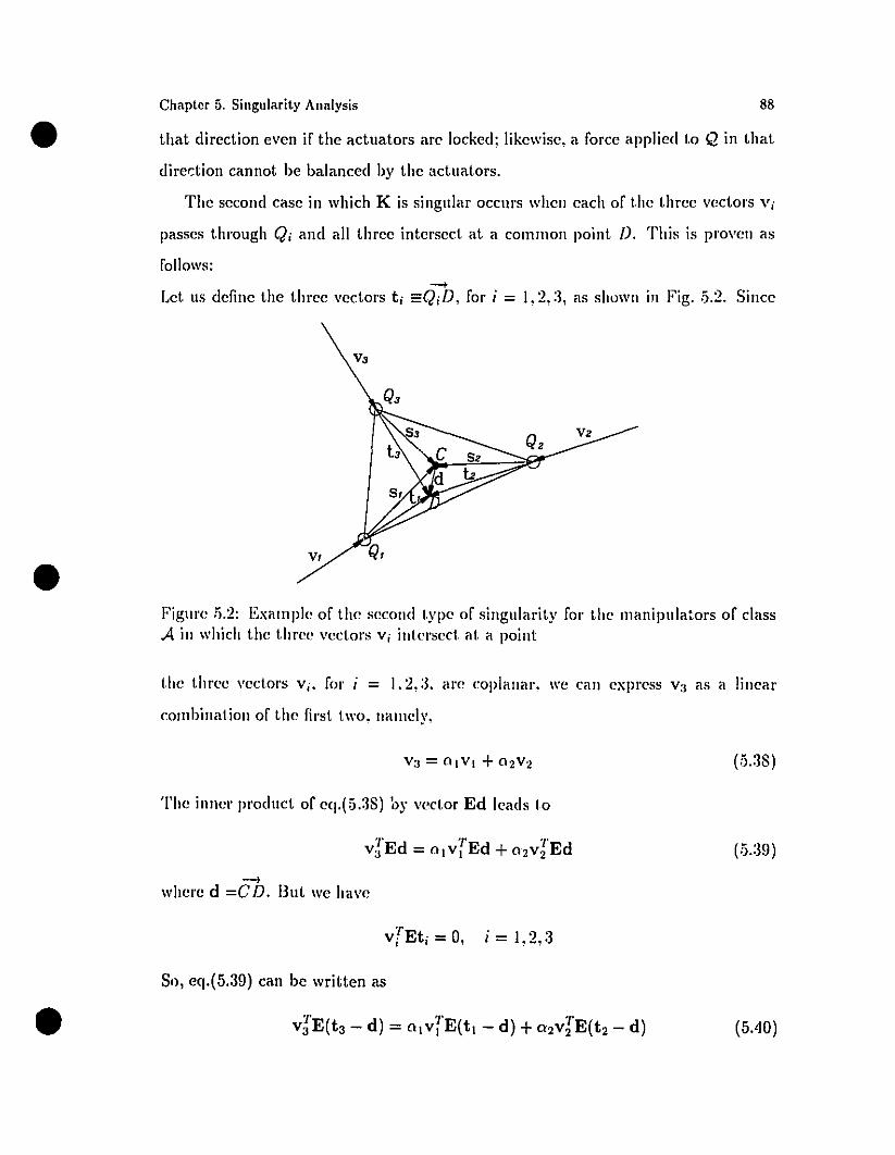
that direction l'ven if the actuators are locked; likewise, a force applied to Q in that

diredion cannot be balanced by the actuators.

The second case in which K is singular occurs wheu each of t.he three vectors Vi

passes through Qi and ail t.hree intersect. at. a common point D. This is proven as

follows:

•Chapter 5. Sil1gularity Al1alysis 88

.....Let us define the three vect.ors ti =.QiD, for; = 1,2,:3, as shown in Fig..5.2. Sincc

• v,

Figure 5.2: Exalllple of t.he second t.ype of singularity for the manipulators of c1assA in which the t.hree vect.ors Vi iulersect. at. a point

t.he t.hrcc vectors Vi. for i = 1,2, :l, arc Coplallar, wc can express Va aS a linear

combination of the first t.wo. namely.

(5.:38 )

•

The inner product. of eq.( 5.:l8) oy Vl'ctor Ed leads to

.....where d =C D. But. wc have

TvjEti=O, ;=1,2,3

Sil, eq.(5.39) can be written as

(5.40)

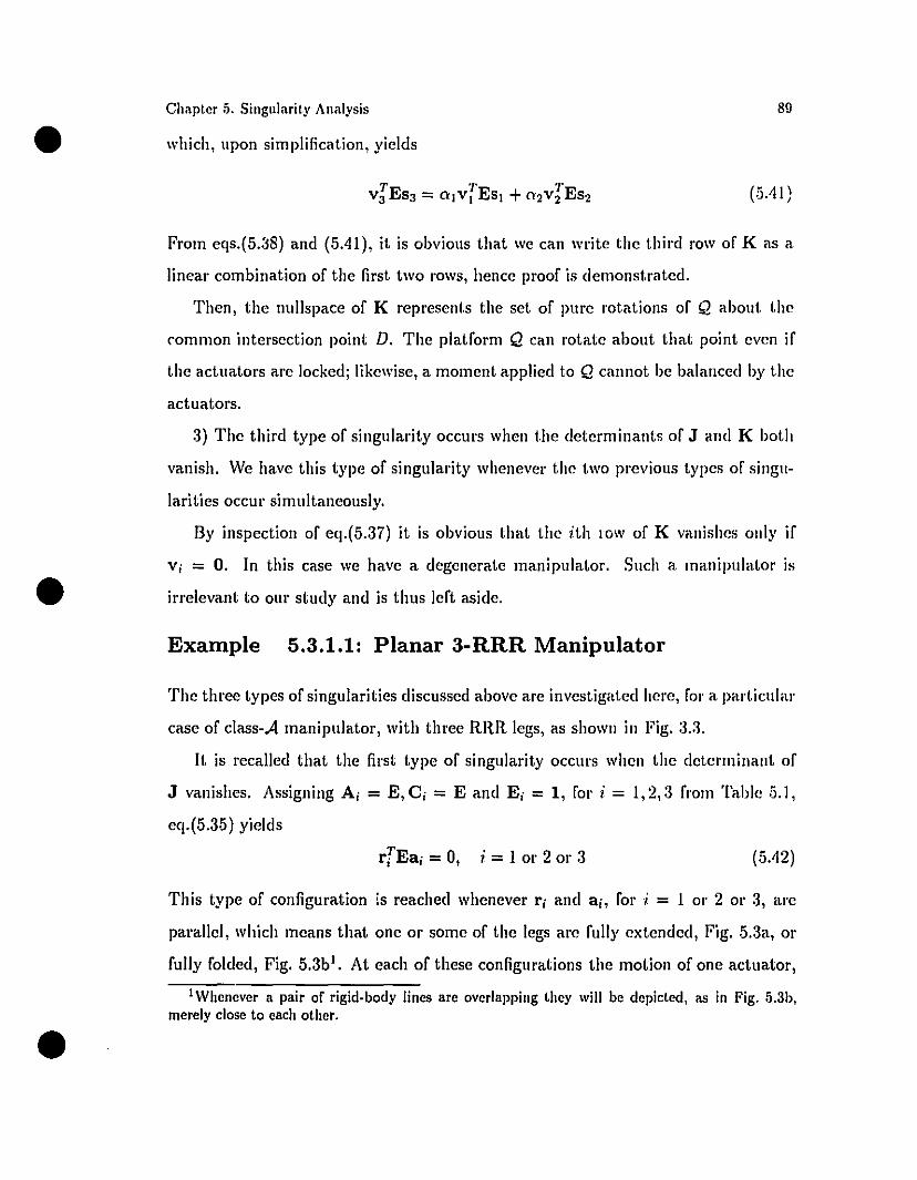
•Chapter 5. Singlliarity Analysis

which, upon simplification, yields

89

(5.41)

•

From eqs.(5.:j8) and (5.41), it is obvious that we can write the thinl row of K as a

linear combination of the first two rows, hence proof is demonstrated.

Then, the nullspace of K represents the set of pure rotations of Q about the

rommon intersection point D. The platform Q can rotate about that point l'ven if

the actuators are locked; likewise, a moment applied 1,0 Q cannot be balanced by the

actuators.

3) The third type of singularity occurs when the determinants of J and K both

vanish. We have this type of singularity whenever the two previous types of singu­

larities occur simultaneously.

By inspection of eq.(5.37) it is obvious that the ith IOW of K vanishes only if

Yi = O. In this case we have a degenerate manipulator. Such a manipulatol' is

irrelevant to our study and is thus left aside.

Example 5.3.1.1: Planar 3-RRR Manipulator

The three types of singularities discussed above are investigated here, fol' a particulal'

case of class-A manipulator, with tlnee RRR legs, as shown in Fig. 3.3.

It is recalled that the first type of singularity occurs when the detenninant of

J vanishes. Assigning Ai = E, Ci = E and E j = 1, for i = 1,2,3 from 'l~"tble 5.1,

eq.(5.35) yields

Tri Eai = 0, i = 1 or 2 or 3 (5.42)

•

This type of configuration :s reached whenever ri and aj, for i = 1 or 2 or 3, are

parallel, which means that one or sorne of the legs are fully extended, Fig. 5.3a, or

fully folded, Fig. 5.3b1• At each of these configurations the motion of one actuator,

1Whenever a pair of rigid-body Iines are overlapping they will be depieled, as in Fig. 5.3b,merely close ta each other.

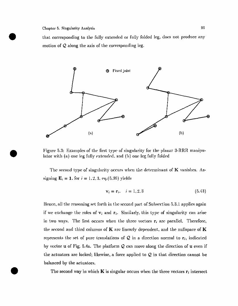
that corresponding to the fully ext.ended or fully folded leg, does not produce any

motion of Q along the axis of the corresponding leg.•Chapler 5. Singniarily Analysis

Cl Fi xpd joinl

DO

•

•

Figure .5.:1: Examples of t.hl' first t.ype of singularity for t.he planar 3-RRH manipu­lator with (a) one leg fully l'xtended. and (h) one leg fully folded

The second type of singularity occu,'S when the determinant of K vanishes. As­

signing E i = 1. for; = 1.2.:1. l'q.(:;.:.lG) yields

Vi=ri. ;=1.2.:3

Bence. ail t.he reasoning set. fort.h in the second part of Suhsection 5.:3.1 applies again

if wc exchange the roics of Vj and rj. Similarly. this type of singularity can arise

in t.wo ways. The first occurs when the three vect.ors ri arc parallel. Therefore.

t.he second and thinl colulllns of K arc linearly dependent. and the nullspace of K

I·epresent.s t.he set. of pure t.ranslat.ions of Q in a direction norlllal to ri. indicated

hy veetor u of Fig. 5.4a. The platforlll Q can 1110ve along the direction of u even if

the aetuators are lockedj likewise, a force applied t.o Q in that direetion cannot be

balanced by the act.uators.

The second way in which K is singular occurs when the three veetors ri interseet

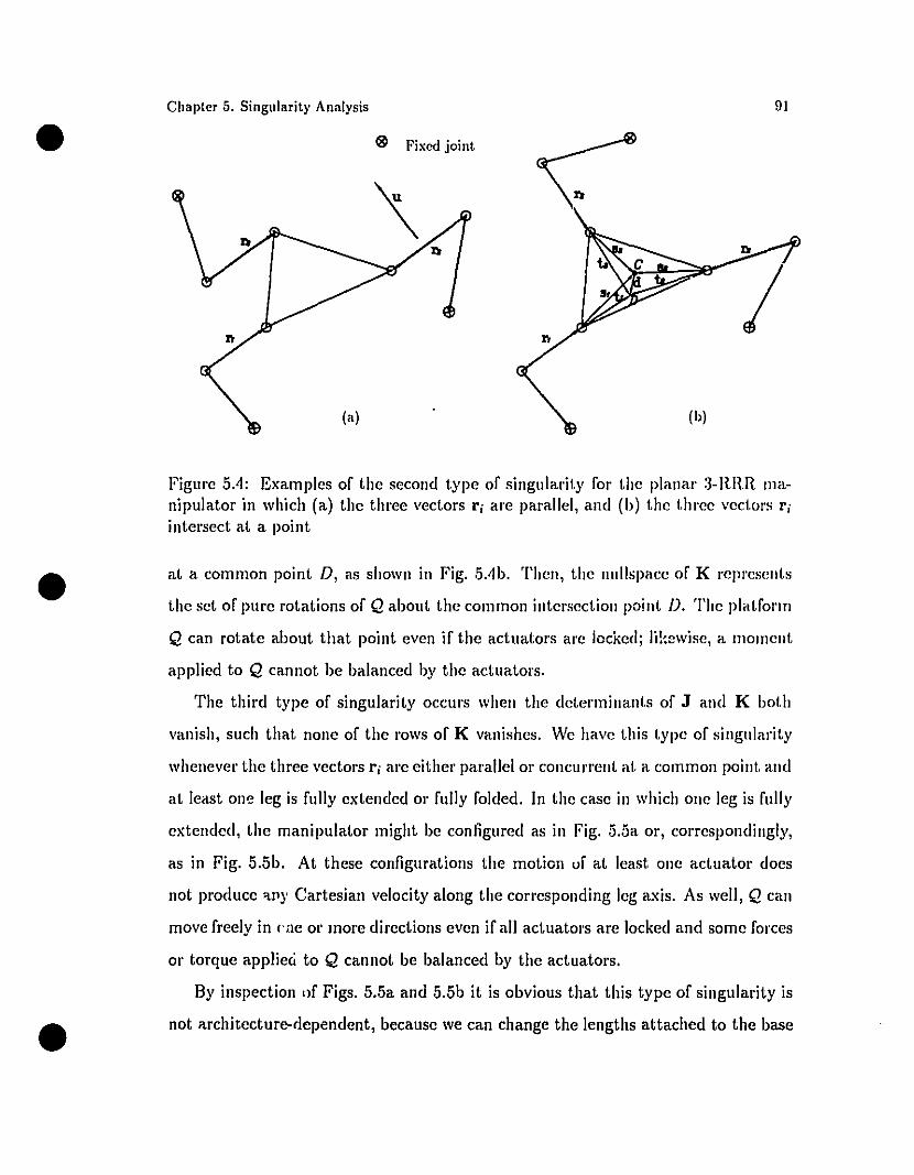
•Chapter 5. Singularity Analysis

~ Fixed joint

(b)

91

1

•

•

Figure .504: Examples of the second type of singularity fol' the planaI' 3-RIUl ma­nipulator in which (a) the three vectors ri arc parallel, and (b) the t.hree vect.ors ri

intersect at. a point.

at. a common point. D, as shown in Fig..5Ab. Thcn, t.hc nullspacc of K rcprescllt.s

t.he set. of purc rot.ations of Q about. t.he common int.crscct.ioll point. /J. The plat.form

Q can rotate about that point even if the actuat.ors arc lockcdj Ii!:ewise, a mOIllCIlt.

applied 1.0 Q cannot be balanccd by the actuators.

The t.hird type of singularity occurs when the dcterminant.s of J alld K bot.h

vanish, such that nonc of the l'OWS of K vanishes. Wc havc this typc of sillgularity

whellever the thrce vectors ri arc either parallcl 01' concurrcnt at. a common point. and

al. least one leg is fully extended 01' fully folded. III thc case in which onc leg is fully

extended, the manipulat.or might be configured as in Fig. 5.5a 01', correspondingly,

as in Fig. 5.5b. At these configurations the motion uf al. Icast. onc act.uat.or does

not pl'Oducc 'Lny Cartesian velocity along the cOl'I'esponding leg axis. As weil, Q can

move freely in ('ne 01' more directions even if ail actuators arc locked and somc forces

01' torque applieci to Q cannot be balanced by the actuators.

By inspection Ilf Figs. 5.5a and 5.5b it is obvious that this type of singularity is

not architecture-rlependent, because we can change the lengths attached 1.0 the base

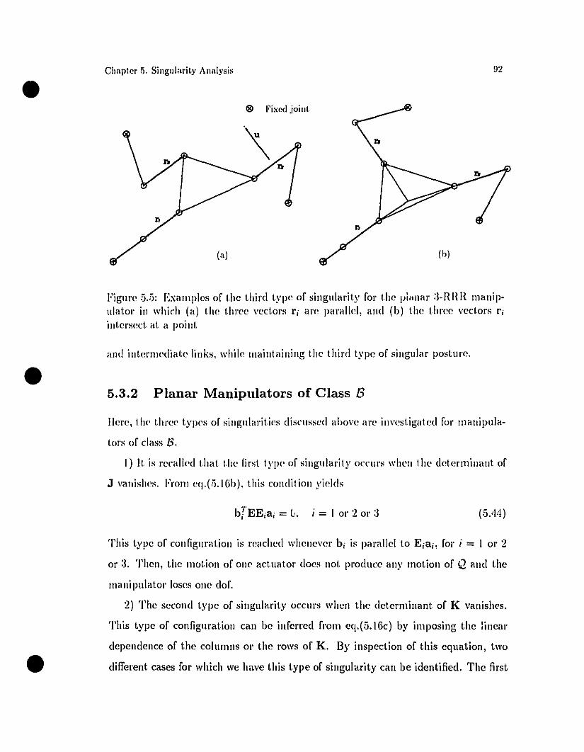
•Chapter 5. SingnJarity Analysis

181 Fixed joi nt

92

•

Figure 5.5: Examples of the thircl type of singularity for the pianar :3-RHR manip­ulator in which (a) the three vectors ri are paralle!, and (h) the three vectors ri

intersect al, a point

and interlllediate links, while lIlaintaining the thinltype of singular posture.

5.3.2 Planar Manipulators of Class B

lIere, ti){' three types of singularities discussed ahove arc investigated for lllauipula­

tors of c1ass B.

J) Il, is recalbl that the first type of singularity occurs when the determinant of

J vanishcs. From eq.(ii.Hih), this condition yields

Tbj EEjai = l" i = 1 or 2 or :3 (5A:l )

•

This type of configuration is reachcd whenever bi is parallcl to Eiaj, for i = 1 or 2

01':3. Then, the motion of one actuator does not producc any motiou of Q and the

manipulator loses one dof.

2) The second type of singularity occurs when the determinant of K vanishcs.

This type of configuration can he inferred from eq.(5.J6c) hy imposing the :inear

dependencc of the columns or the rows of K. By inspection of this equation, twu

different cases for which we have this type of singularity can he identified. The first

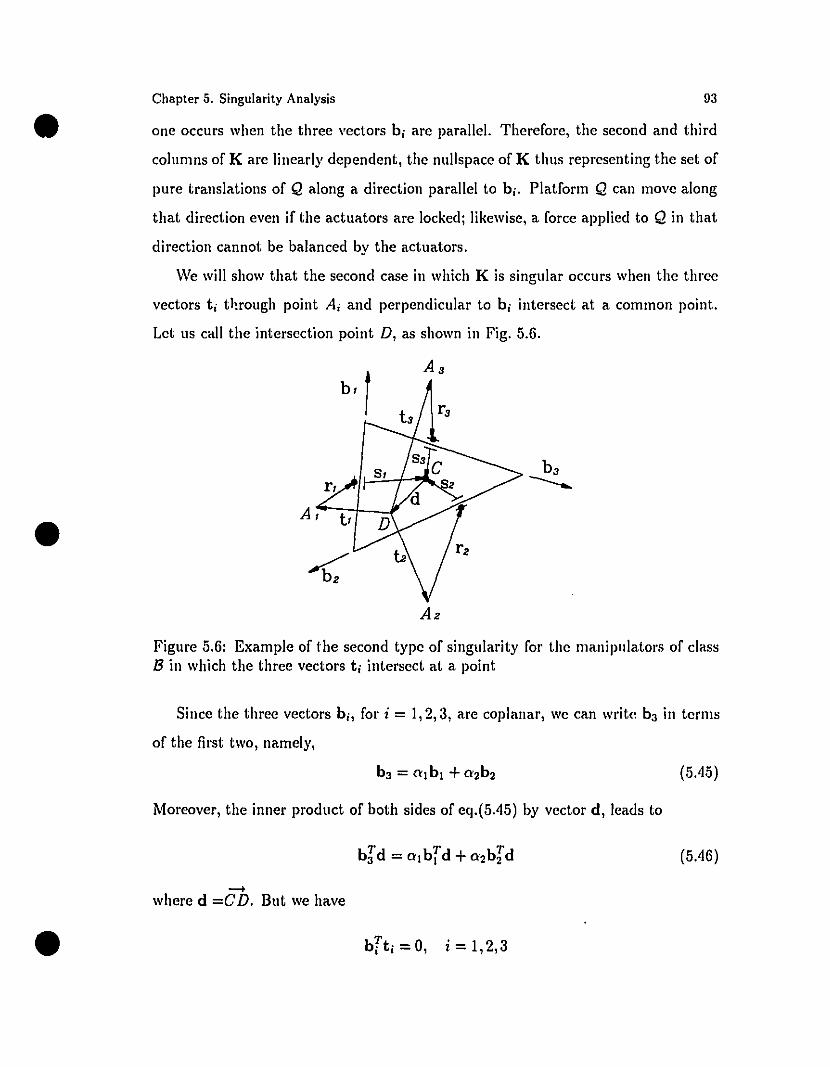
one occurs when the three "ectors b i arc paralleI. Therefore, the second and third

columns of K arc linearly dependent, the nullspace of K thus representing the set of

pure translations of Q along a direction parallel to bi. Platform Q can mo"e along

that direction even if the actuators arc locked; likewise, a force applied to Q in that

direction cannot be balanced by the actuators.

Wc will show that the second case in which K is singular occurs when the three

"ectors ti th.rough point Ai and perpendicular to bi intersect at a common point.

Let us cali the intersection point D, as shown in Fig. 5.6.

•

•

Chapter 5. Singularity Analysis

At b

93

Az

Figure 5.6: Example of the second type of singularity for the manipulators of dassB in which the three vectors ti intersect at a point

Since the three vectors bi, for i = 1,2,3, are coplanar, we can writc ba in terms

of the first two, namely,

(5.45)

Moreover, the inner product of both sides of eq.(5.45) by vector d, leads to

(5.46)

•-+

where d =CD. But we have

b;ti=O, i=1,2,3

•Chapter 5. Singularity Analysis

Then, eq.(5.46) can be written as

(5.4ï)

l\1oreover, wc have

cl + t j = -(rj + sil, i = 1,2,a

Substituting the values of cl + t j , for i = 1,2. a, from the foregoing equation iuto

eq.(.5.4ï), yiclds

(5.48)

•

•

Moreover, from eq.(5.45), il. is apparent that

(.5.49)

From eqs.(.5.·18) and (5.49). il. is obvious that one can write the third row of K

as a !inear combination of the first two rows. thereby complcting the proof.

Then, the nullspacc of K represents the set of pure rotations of 12 about the

common intersection point /J. The platform 12 can thus rotate about tl.at point even

if the actuators arc locked; likewise. a moment applied 1.0 12 cannot be baJanccd by

the actuators.

:1) The thil'(! type of singularity OCClll'S when the determinants of J and K both

\'anish. This type of singularity occnl's whenever the two types of singuJarities arises

si mul taneously.

Inspection of eq.(5.16c) reveals that the rows of K cannot vanish, because Ilbili =

1. for i = J, 2, a.

Example 5.3.2.1: Planar DT Manipulator

The tlll'ee types of singularities discussed above arc investigated here for a special

type of cJass-B manipulator that has three PRP legs. namely the dOllble-ll'ianglllal'

(DT) manipulator shown in Fig. 3.5.

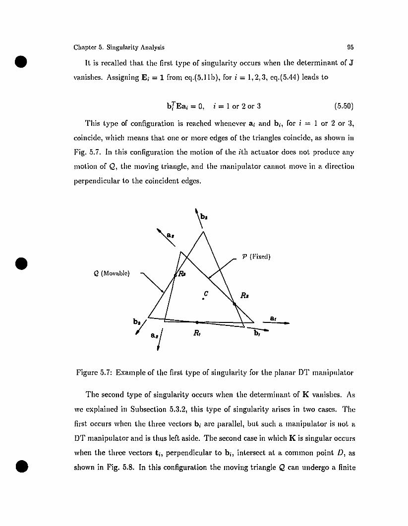
It is recalled that the first type of singularity occurs when the determinant of J

vanishes. Assigning Ei = 1 from eq.(5.llb), for i = 1,2,3, eq.(5.44) leads to•Chapter 5. Singnlarity Analysis 95

bTEai = 0, i = 1 or 2 or 3 (5..50)

This type of configuration is reached whenever ai and bi, for i = 1 or 2 or 3,

coincide, which means that one or more edges of the triangles coincide, as shown in

Fig. 5.i. In this configuration the motion of the ith actuator does not producc any

motion of Q, the moving triangle, and the manipulator cannot move in a direction

perpendicular to the coincident edges.

'"~.

• P (Fixed)

Q (Movable)

C R••

bja,

aiR, b, -

Figure .5. i: Example of the first type of singularity for the planaI' DT manipnlator

•

The second type of singularity occurs when the determinant of K vanishes. As

we explained in Subsection 5.3.2, this type of singularity arises in two cases. The

first occurs when the tlll"ee vectors b i are parallel, but such a manipulator is not a

DT manipulator and is thus left aside. The second case in which K is singular occurs

when the three vectors ti, perpendicular to bi, intersect at a common point D, as

shown in Fig. 5.8. In this configuration the moving triangle Q can undergo a finite

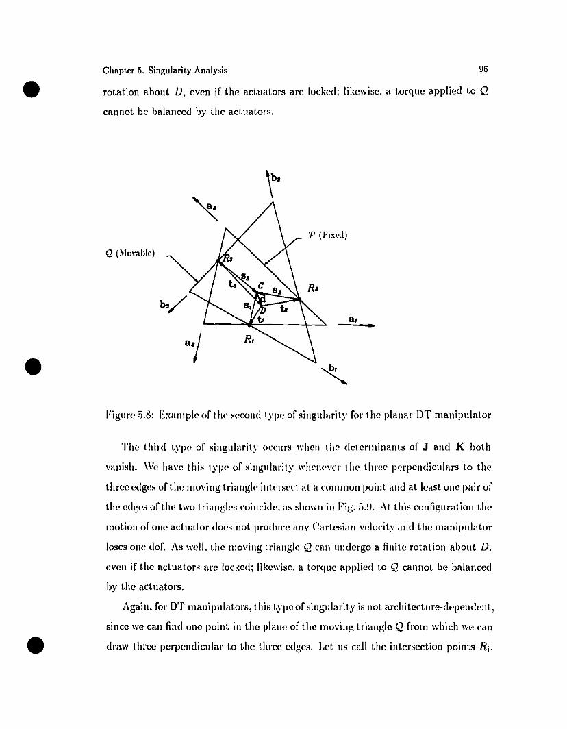
•Chapter 5. Singularity Analysis rJ6

rot.ation about D, even if the act.uators arc locked; !ikewise, a torque applied t.o Q

cannot be balanced by t.he act.uat.ors.

•

Q (Mm'ahle)

op (l'ixed)

•

Figun' 5.S: E)o;alllple of th,' second type of singularity for the planaI' DT manipulator

The t.hinl t.ype of singularity OCC\II'S when the deterlllinants of J and K bot.h

vanish. Wc have t.his Iype of singularity wlwncvcr the thrce perpendiculars to t.he

t.lll·cc edges of the lIIoving triangle intl'rs('ct al a mll1lllon point. and at. least. on<' pair of

the edges of t.he two triangles mincide, as shown in Fig. 5.D. :\t. t.his configurat.ion t.he

lIIot.ion of one aduator does not producc any Cartesian \'<,loeity and the Illanipulator

loses one dof. As weil, the Illoving triangle Q can undergo a finite rotation about /J,

even if t.he aduators are locked; likewise, a torque applied to Q cannot be balanccd

by t.hc act. uat.ors.

Again, fOl' DT Illanipulat.ors, t.his typc of singularity is not architccture-dependent,

since we can find one point in the plane of the moving triangle Q from which we can

draw t.hree perpendicular t.o the three edges. Let. us cali the intersection points Ri,

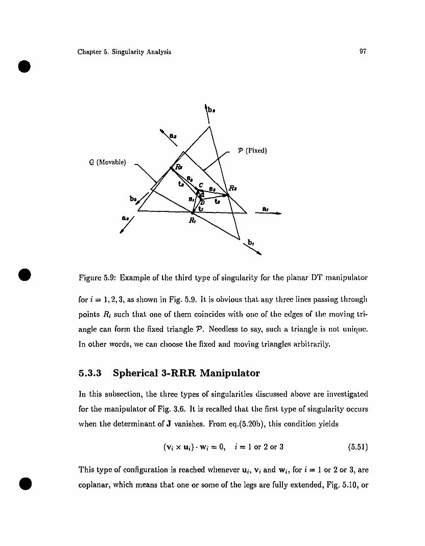
Figure 5.9: Example of the third type of singularity for the planaI' DT manipulator

•

•

Chapter 5. Singularity Allalysis

Q (Movable)

7

op (Fixed)

a,•

9i

for i = 1,2,3, as shown in Fig. 5.9. It is obvious that any three lines passing throngh

points Ri such that one of them coincides with one of the edges of the moving tri­

angle can form the fixed triangle 'P. Needless to say, snch a triangle is not unique.

In other words, we can choose the fixed and moving triangles arbitrarily.

5.3.3 Spherical 3-RRR Manipulator

In this subsection, the three types of singularities discnssed above are investigated

for the manipulator of Fig. 3.6. It is recalled that the first type of singularity occnrs

when the determinant of J vanishes. From eq.(5.20b), this condition yields

This type of configuration is reached whenever Ui, Vi and Wi, for i = 1 or 2 or 3, are

coplanar, which means that one or sorne of the legs are fully extended, Fig. 5.10, or•(Vi x Ui)' Wi =0, i =1 or 2 or 3 (5.51 )

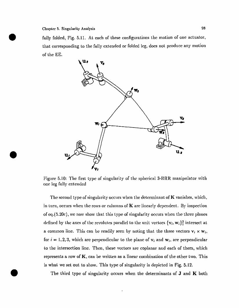
fully folded, Fig. 5.11. At each of these configurations the motion of one actuator,

that corresponding to the fully extended or folded leg, does not producc any motion

of the EE.

•

•

Chapter 5. Singularity Analysis 98

Ua

•

Figure 5.10: The first type of singularity of the spherical 3-HRH manipnlator withone Icg fully ex(ended

The second type of singulllri(y occlll's when the determinant of K vlInishes, which,

in tUI'll, occurs when thc rows or columlls of K arc linellrly dcpcndcnt. By inspection

of cq.(5.20c), wc nOlI' show that this t.ype of singularity occurs when thc three plancs

defincd by thc axcs of the rCI'olutes parallcl to the unit vectors {Vi, wd~ intersect at

a common Hnc. This can be readily seen by noting that the three vectors Vi x Wi,

for i = 1,2,3, which arc perpcndicular to the plane of Vi and Wh arc perpendicular

to the interscction Hnc. Thcn, these vectors arc coplanar and each of them, which

represents a row of K, can be written as a !inear combination of the other two. This

is what we set out to show. This typc of singularity is depicted in Fig. 5.12.

The third type of singularit.y occurs when the determinants of J and K both

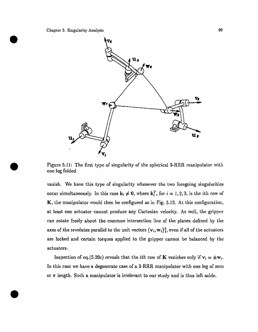
Figure 5.11: The first type of singularity of the spherical 3-RRR manipulator withone leg folded

•

•

Chapter 5. Singularity Analysis

v..

u ..

99

•

vanish. We have this type of singularity whenever the two foregoing singularitics

occur simultaneously. In this case kj # 0, where kT, for i = 1,2,3, is the ith row of

K, the manipulator would then be configured as in Fig. 5.13. At this configuration,

at least one actuator cannot produce any Cartesian velocity. As weil, the gripper

can rotate freely about the common intersection line of the planes defined by the

axes of the revolutes parallel to the unit vectors {Vi, Win, even if ail of the actuators

are locked and certain torques applied to the gripper cannot be balanced by the

actuators.

Inspection of eq.(5.20c) reveals that the ith row of K vanishes only if Vj = ±Wj.

In this case we have a degenerate case of a 3-RRR manipulator with one leg of zero

01' 11' length. Such a manipulator is irrelevant to our study and is thus left aside.

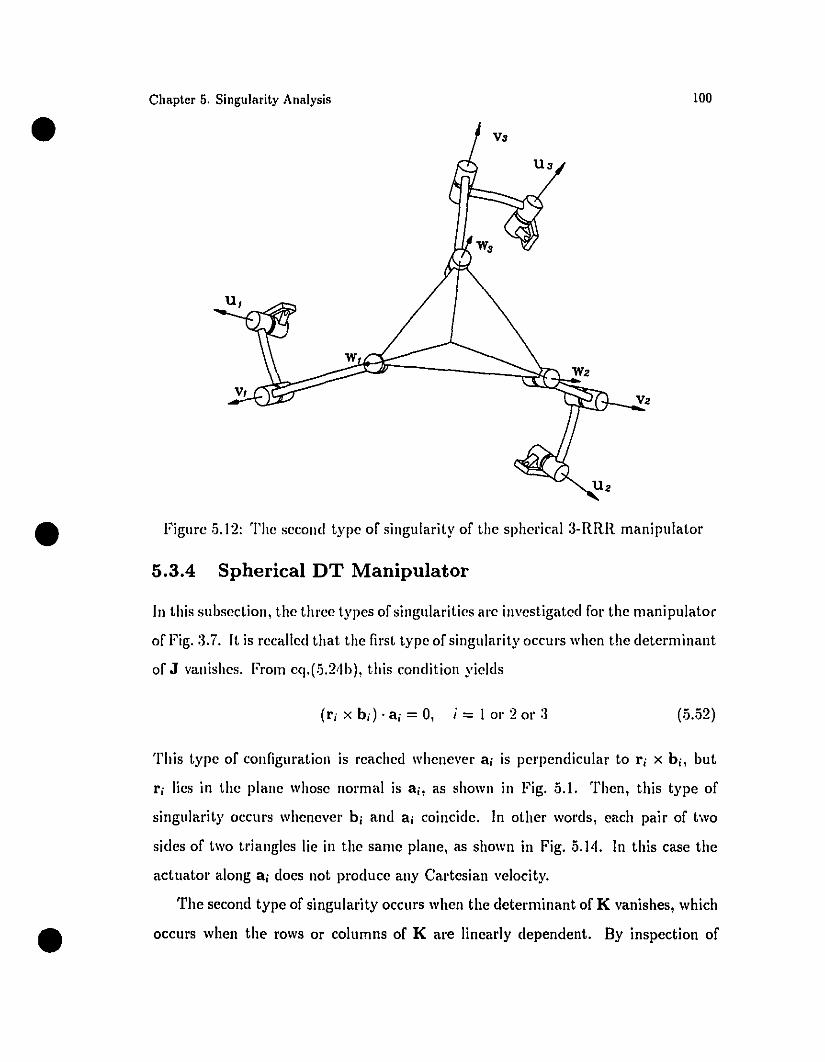
Figure 5.12: The second type of singularity of the spherical 3-RRR manipulator

•

•

Chaptcr 5. Singularity Analysis

w,

'rI'-.Lr--..;Vz

100

5.3.4 Spherical DT Manipulator

ln this subsection, the three types of singularities are investigated for the manipulator

of Fig. :3. ï. It is recalled that the first type of singularity occurs when the determinant

of J vanishes. From eq.(5.24b), this condition yields

(ri x b;) . ai = 0, i = 1 or 2 or :3 (- -?)0).0)_

•

This type of configuration is reached whenever ai is perpendicular to ri x b i , but

ri lies in the plane whose normal is ai, as shown in Fig. 5.1. Then, this type of

singularit)' occurs whenever b i and ai coincide. In other words, each pair of two

sides of two triangles lie in the saille plane, as shown in Fig. 5.14. In this case the

actuator along ai does not produce an)' Cartesian velocity.

The second type of singularity occurs when the determinant of K vanishes, which

occurs when the rows or columns of K are linearl)' dependent. By inspection of

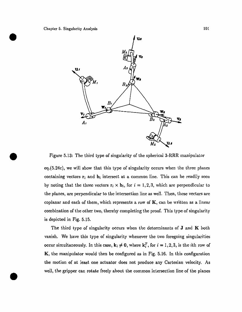
Figure 5.13: The third type of singularity of the spherical 3-RRR manipulator

•

•

Chapter 5. Singularity Analysis

Ut

At

101

•

eq.(5.24c), wc will show that this type of singularity occurs when the three planes

containing vectors ri and bi intersect at a common line. This can be readily seen

by noting that the three vectors ri x bi, for i = l, 2,~, which are perpendicular to

the planes, are perpendicular to the intersection line as weil. Then, these vectol'S are

coplanar and each of them, which represents a l'OW of K, can be written as a linear

combination of the other two, thereby completing the pl'oof. This type of singularity

is depicted in Fig. 5.15.

The third type of singularity occurs when the determinants of J and K both

vanish. Wc have this type of singularity whenever the two foregoing singularities

occur simultaneously. In this case, ki #- 0, where kT. for i =1,2,3, is the ith row of

K, the manipulator would then be configured as in Fig. 5.16. In this configuration

the motion of at least one actuator does not producc any Cartesian velocity. As

weil, the gripper can rotate freely about the common intersection line of the planes

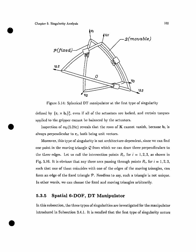
•CI.apter 5. Singularity Analysis

VI

;p(jixed)

U2

V2

.2 (movable)

102

•

•

Figure 5.14: Spherical DT manipulator at the first type of singularity

defined by {f; x b;H, e"en if ail of the actuators are locked. and ccrtain torques

"l'l'lied to t.he gripper cannot be balanccd by the actuators.

Inspection of eq.(5.24c) re"eals that the rows of K cannot vanish, because b i is

always perpendicular t.o fi, both being unit vectors.

Moreover, this type of singularity is not architecture-dependent, since we can find

one point in the moving triangle Q from which we l'an draw three perpendiculars to

the tJ.rcc edges. Let. us cali the intersection points R;, for i = 1,2,:J, as shown in

Fig. 5.16. It is obvious that any three arcs passing through points R;, for i = 1,2,:J,

such that one of them coincides with one of the edges of the moving triangles, can

fonTI an edge of the fixed triangle P. Needless to say, such a triangle is not unique.

ln other words, we can choose the fixed and 1110ving triangles arbitrarily.

5.3.5 Spatial 6-DOF, DT Manipulator

ln this subsection, the three types of singularities are investigated for t.he manipulator

introduccd in Subsection :J.4.1. It is recalled that the first type of singularity occurs

•

•

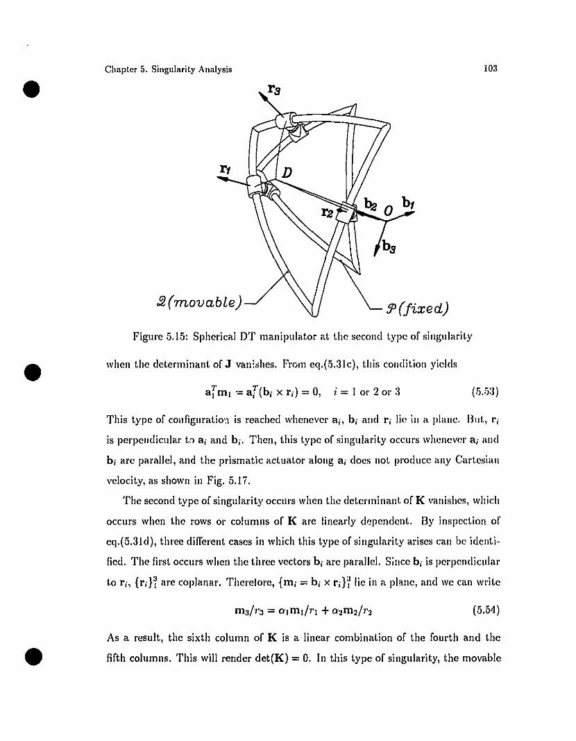
Chaptcr 5. Singularity Analysis

f2(movable)

Figurc 5.15: Sphcrical DT manipulator at thc sccond typc of singularity

whcn thc dctcrminant of J van:shcs. From cq.(.5.31c), this condition yiclds

103

7' Ta) ml -= ai (bi x ri) = 0, i = 1 or 2 or 3 (5.5:l)

•

This typc of configuratio'.l is rcachcd whcncvcr ai, bi and ri lic in a planc. But., ri

is pcrpcndicular tCl ai and bi. Thcn, this typc of singularity occurs whcncver ai all<l

bi arc parallcl, and the prismatic actuator along ai docs not producc <Lny Cartesian

velocity, as shown in Fig. 5.17.

Thc second type of singularity OCClll'S whcn the determinant of K vanishes, which

occurs when thc l'OWS or co!umns of K are lincarly d~pcndcnt. By inspcction of

cq.(5.31d), three different cascs in which this type of singularity ariscs can be idcnti­

ficd. The first occurs when the three vectors b i arc parallci. Sincc b i is pcrpcndicular

to ri, {rin are coplanar. Thcrelore, {mi =bi x r;}? lic in a planc, and wc can write

(5.54)

As a resu)t, the sixth column of K is a linear combination of the fOUl-th and the

fifth co)umns. This will rendel' det(K) =O. In this typc of singularity, the movable

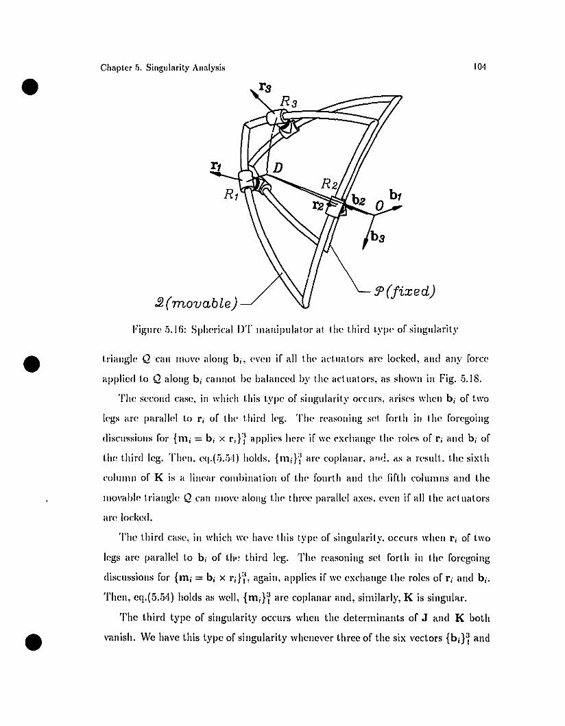
•Chapler ;i. Singularily Analysis

.!î(movable)

101

•

•

Figlll'e 5.1 fi; Spherical DT lIlallipulator al 1he t.hinl t.ype of siugularity

t.riallgle Q cali IIlllVe alollg b i . eVell if ail th" actllators are locked, aud allY force

applied t.o Q alollg b i ca Il ilOt. he balanced by t.he actualors, as showu in Fig. 5.18.

The secolld case, in which this t.ype of sillgularity occnrs. arises when b i of two

legs are paralle! t.o ri of the t.hinl leg. The reasonillg set fort.h ill 1he foregoing

discussiolls for {mi = b i x l'in appli"s here if we cx<'!lang<' t.h" roles of ri aud bi of

t.he t.hinl leg. Th"n. eq.(5.5'1) holds. {m,}'! an' copia liaI'. alld. as a n'still.. t.he sixth

COhllll1l of K is a linear cOlllbinatilln of t.he fOlll'lh a11<1 the fifth colulllns and t.he

nlovahl" triangle Q can 11I00'e alon~ t.11<' th1'<'e parallel axes. eVl'n if ail the acl uators

are locked.

The t.hinl case, iu which Il'e have this typ<~ of singularity. occurs when ri of t.wo

legs are paralle! t.o b i of t.h,~ thinl leg. The reasouÎng sel fort.h in t.he foregoing

discussions for {mi = bi x l'if!, agaiu, applies if Wl' l'xchauge t.he l'ales of ri aud bi.

Then, eq.(5.5'1) holds as weil, {min are coplanar aud, silllilarly, K is singular.

The thinl type of singularity occurs when the deterlllinauts of J and K bath

vanish. Wc have this type of singularity whenevel' th rel' of the six vectors {birl and

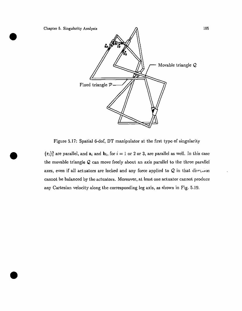
105

Movable triangle Q

Fixed triangle P----./

Chapt.er 5. Singularity Analysis

•

•Figure 5.17: Spatial 6-dof, DT manipulator at the first type of singularity

{rin are pal'allel, and ai and bi, for i = 1 or 2 or 3, are parallel as weil. In this case

the movable triangle Q can move freely about an axis parallel to the three parallel

axes, even if all actuators are locked and any force applied to Q in that dil"rC';'ll1

cannot be balanced by the aetuatol's. Moreover, at least one actuator cannot produce

any Cartesian velocity along the corresponding leg axis, as shown in Fig. 5.I!).

•

•

•

•

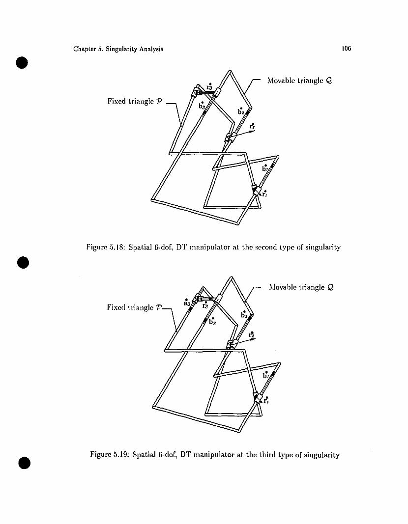
Chapter 5. Singularity Analysis

Movable triangle Q

Figure 5.18: Spatial 6-dof, DT manipulator at the second type of sillgularity

Movable triangle Q

Figure 5.19: Spatial 6-dof, DT m<tllipulator at the third type of singularity

lOG

•

•

•

Chapter 6

Isotropie Designs

6.1 Introduction

The concept of manipulator isotropy, based on the condition numbers of the .Jaco­

bian matrices, is now explained, as pertaining to parallel manipulators. Using this

concept, the isotropie designs of two general classes of planaI' parallel manipulators,

of spherical DT and 3-RRR parallel manipulators, and of spatial 6-dof, DT mecha­

nism, introduced in Chapter 3, are found. Having derived the Jacobian matrices of

the manipulators, in an invariant form in Chapter 5, al!ow us to find al! isotropie

designs.

6.2 Isotropie Designs

Mechanism control accuracy depends upon the condition number of the Jacobian

matrices J and K. The condition number is based on a concept common to al!

matrices, whether square or not, i.e., their singular values. For an m x n matrix

A, with m < n, we can define its m singular values as the non-negative square

l'oots of the non-negative eigenvalues of the m x m matrix AAT. Because AAT is

square, symmetric and at !east positive-semidefinite, its eigenvalues are ail real and

non-negative. Also, if the matrix under investigation is dimensional!y homogeneous

which, in our case, happens for J and K only in the spherical case, then we can

meaningful1y order the singular values of these matrices from smallest to largest.

If, on the other hand, these matrices are not dimensionally homogeneous, which

is the case for planaI' and spatial tasks involving both positioning and orienting,

or manipulators with both prismatic and revolute actuators; then we can redefine

these matrices by recalling the concept of ehamete/'istie length, first introducerl in

(Tandirci et aL, 1992), and dividing the e1ements that have units of length by this

quantity. Therefore, we can always produce a dimensionally-homogeneous .Jacobian

matrix, which enablcs a meaningful ordcring of its singular values from smallest to

largest. Thus, if am and aM denotc the smallest and the largest singular valucs of a

matrix, its condition numbcr is thcn defincd as

and hcnce, thc larger the variancc of thc singular values, thc larger thc condition

number. Thc significance of thc condition number of a matrix pertains to the nu­

mcrical invcrsion of this matrix when solving a systcm of lincar equations associated

with the matrix. Cleal'iy, in the casc of non-square matrices, this inversion is un­

dcrstood as a genel'llli:etf Ï1weI'Siorl. Indeed, when inverting a matrix with finite

precision, a rOllndoff error is always present, and hence, a roundoff-error amplifica­

tion arrccts thc accuracy of the computed results. Fllrthermore, this amplification

is bounded by the condition number of thc matrix. It is apparent that a singular

matrix has a minimulll singular value of zcro, and hence, its condition numbcr be­

comes infinite. Converscly, if the singular values of a matrix are identical, then the

condition number of thc matrix attains a minimum value of unity, matrices with such

a pruperty being calleel isotropie. The reason why isotropic matrices are desirable is

that they can be inverted at no cost because the inverse of an isotropic matrix, or

the generalized inverse of a rectangular isotropic matrix for that matter, is propor­

tional to its transpose, the proportionality factor being the reciprocal of its multiple

singular value.

•

•

•

Chapter 6. Isotropie Designs

1'(8) == aMO"m

\08

(6.1 )

6.2.1 Planar Manipulators of Class A

From the above discussion, and considering that the Jacobian matrices are

configuration-dependent, it is apparent that the condition number of the Jacobian

matrices of a manipulator is configuration-dependent as weil, and hence, a manipu­

lator can be designed with an architecture that allows for postures entailing isotropie

Jacobian matrices, such a design being called isotropie. However, this property disap­

pears in ail other postures. This is a fact of life and nothing can be done about it, but

one can design for postures that are isotropie, and then plan tasks that lie weil within

a region where th·.; condition number is acceptable. For manipulators with isotropie

designs, such regions coYer a substantial percentage of the overall workspace, the

condition number degenerating only for postures very close to singularities, which

should be avoided in trajectory planning, in any event.

Below we will find the isotropie designs of several manipulators introduced in

Chapter 3.

•

•

Chapter 6. Isotropie Designs 109

In this subsection we find isotropie designs for planar manipulators of class A. It

is recalled that a design is isotropie if both J and K are isotropie, i.e., if positive

scalars 0' and r exist such that

JJT = 0'21

KKT = r 21

(6.2a)

(6.2b)

•

where J and K are given in eqs.(5.9b) and (5.9c), respectively. But J is not

dimensionally-homogeneous if we have different types of actuators, i.e., if sorne ac­

tuators are revolute and the others are prismatic. If this is the case, in order to

render J dimensionally-homogeneous we divide the ith column of J by a length li,

the characteristic length of the ith leg of the manipulator, understood here as defined

•Chapter 6. Isotropie Designs

in (Tandirci ct al., 1992) for seriai manipulators, and redefine J as

rfEI(Alal +Clrtl/ll 0 0

J t- 0 rfE2(A2a2 +C2r2)/l2 0

o 0 rIE3(A3a3 +C3r3)/l3

110

(6.3)

•

where li = 1, for i = 1,2,3, if wc have the same lypes of aclualors in ail legs or the

acluatOl" of the ith leg is prismatic.

Matrix K is not dimensionally-homogeneous either. To render K dimensionally­

homogeneous we divide the first column of K by a length L, the characteristic length

of the manipulators, and redefine the .Jacobian K as

rfE1Esl/L '1'-ri El

Kt- '1' '1' (6,4 )r2E2EsdL -r2E2

'1' / '1'1'3 E3ES3 L -r3 E3

Snbstitution of the values of J and K of eqs.(6.:J) and (6..1) into eqs.(6.2a) and

(6.2b), respeclive1y, npon silliplification yiclds

(6.5a)

and

(6.5b)

•where ai and bi, for i = 1,2,3, are defined as

'1'a· = r· E·Es·1- 1 1 1

'1'bi == Ei ri

(6.5c)

(6.5d)

Equations (6.5a) and (6.5b) lead to the conditions for isotropie design of this dass

of manipulators, namely,•Chaptcr 6. Isotropie Designs

(bi(Atal +C t rd/ld2 = 0'2

(bf(A2a2 +C2r2)/l2f = 0'2

(bI(A3a3 +C3r3)/l3)2 = 0'2

bibl = bfb2 = bIb3p2

q+ L2 = 0

111

(6.6a)

(6.6b)

(6.6e)

(6.6d)

(6.6e)

•

where

and henee

2L2 = !!­

-q

l,. = 1,1 bTtAi aO'i+Cir;} Il,' 2 31 = l, ,

Example 6.2.1.1: Planar 3-RRR Manipulator

(6.6f)

(6.6g)

(6.ïa)

(6.ïb)

Here, we find isotropie designs for a partielliar case of dass-A maniplliator, with

three RRR legs, as shown in Fig. 3.3. The isotropie design of this maniplliator

has been addressed in the literature, namely, by Gosselin (1988) and Gosselin and

Angeles (1988). By resorting to numerieal methods, they found a number of disercte

isotropie designs for the manipulator.

Assigning Ai = E, Ci = E, Ei = 1, from Table 5.1, and li = l, for i = 1,2,3, the

conditions for isotropie design, namely, eqs.(6.6a-e) yield

•(6.8a)

(6.8b)

(6.8e)

Equations (6.8a- 6.8e), the conditions for isotropie design, produce manipulators

with the following characteristics:

1) The base and the EE triangles are equilateral and share a eommon centroid at

the isotropie configuration;

2) corresponding leg links have the same length;

3) the angles between the leg links arc equal.

The foregoing characteristics lead to a three-parameter continuum for isotropie

designs of the manipuiator. The three-dimensional design parameters p, a and {3 are

defined as follows:

•

•

Chapter 6. Isotropie Designs

where

ai = rTEsi = p, i = 1,2,3

T T Tri r2 = ri ra = r2ra = q

Cl = lIadl = lIa211 = IlaaliIIrdl II r211 lira Ilp=-=-=-

Cl Cl (l

lEa=­

Cl

{3 = IFCl

112

(6.8d)

(6.8e)

(6.9)

where lE and IF arc the side lengths of the EE and the fixed triangles, respectively.

The continuum of isotropie designs is given as

o:5a< 00

But the condition for feasibility of the design leads to the only constraint, i.e.,

•

o:5{3< 00

o:5p< 00

V3(a-{3) < 13(p+1) -

(6.10)

(6.11)

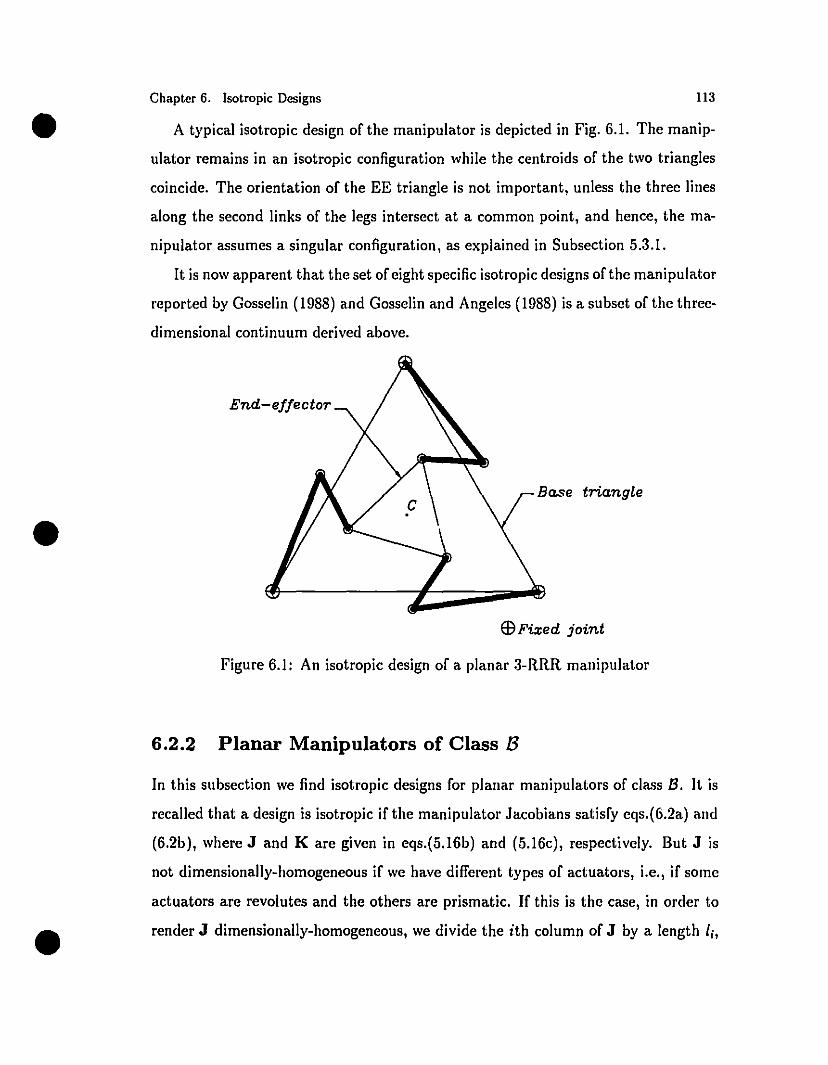
A typical isotropie design of the manipulator is depicted in Fig. 6.1. The manip­

ulator remains in an isotropie configuration while the centroids of the two triangles

coincide. The orientation of the EE triangle is not important, unless the three lines

along the second links of the legs intersect at a common point, and hence, the ma­

nipulator assumes a singuIar configuration, as explained in Subsection 5.3.1.

It is now apparent that the set of eight specifie isotropie designs of the manipulator

reported by Gosselin (1988) and Gosselin and Angeles (1988) is a subset of the three­

dimensional continuum derived above.

•

•

Chaptcr 6. Isotropie Designs

End-effeotor

113

•

$Fixed joint

Figure 6.1: An isotropie design of a planar 3-RRR maniplliator

6.2.2 Planar Manipulators of Class B

In this sllbsection we find isotropie designs for planar manipulators of class 8. It is

recalled that a design is isotropie if the manipulator Jacobians satisfy eqs.(6.2a) and

(6.2b), where J and K are given in eqs.(5.16b) and (5.16c), respectively. But J is

not dimensionally-homogeneous if we have different types of actuators, i.e., if sorne

actuators are revolutes and the others are prismatic. If this is the case, in order to

render J dimensionally-homogeneous, we divide the ith column of J by a length li,

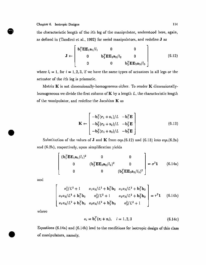
the characteristic length of the ith leg of the rnanipulator, understood here, again,

as defined in (Tandirci et al., 1992) for seriai rnanipulators, and redefine J as•Chaptcr 6. Isotropie Designs

biEE1al/11 0 0

J i- 0 bfEE2a2/12 0

or /o 0 b3EE3a3 13

114

(6.12)

where li = 1, for i = 1,2,3, if we have the sarne types of actuators in ail legs or the

actuator of the ith leg is prisrnatic.

Matrix K is not dirnensionally-homogeneous either. To render K dirncnsionally­

homogencous we divide the first column of K by a length L, the charactel'istic length

of the manipulator, and redcfinc the .Jacobian K as

•Ki-

-biE

_bTE2

-bfE

(6.13)

•

Substitution of thc valucs of J and K from cqs.(6.12) and (6.1:3) into cqs.(6.2a)

ami (6.2b), rcspcctivcly, upon simplification yiclds

(biEE1atl1d2 0 0

0 or 2 0 = ".21 (6.l4a)(b2 EE2a2/12)

0 0 (bIEE3a3/13j2

ami

(lfll} + 1 / 2 b·r / 2 b1·(11(/2 1- + 1b2 (11(13 1- + 1b3

2 T aYU + 1 / 2 b1· = r21 (6.14b)(11(12/1- + b l b2 (12(13 1- + 2 b3/ 2 ·r / 2 T (15/ [} + 1(11(131- +b,b3 (12(13 1- + b2 b3

whcre

T i = 1,2,3 (6.l4c)(Ii = b i (ri + sd,

Equations (6.14a) and (6.14b) lead to the conditions for isotropie dcsign ofthis class

of rnanipulators, narnely,

•

•

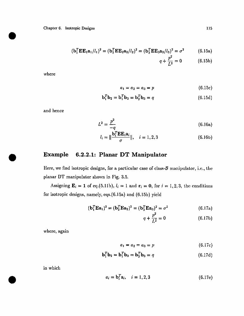
Chapter 6. Isotropie Designs

where

and hence

Example 6.2.2.1: Planar DT Manipulator

115

(6.15a)

(6.15b)

(6.l.5c)

(6.1.5d)

(6.16a)

(6.16b)

Here, we find isotropie designs, for a particu1ar case of class-B manipulator, i.e., the

planar DT manipulator shown in Fig. 3..5.

Assigning Ei = 1 of eq.(.5.lIb), li = 1 and ri = 0, for i = 1,2,3, the conditions

for isotropie designs, namely, eqs.(6.1.5a) and (6.I.5b) yie1d

(6.17a)

(6.17b)

where, again

•in which

C1i=bTsi, i=I,2,3

(6.17c)

(6.17d)

(6.17e)

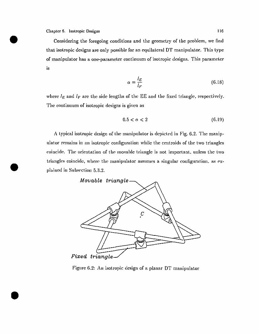
Considering the foregoing conditions and the geometry of the problem, we find

that isotropie designs are only possible for an equilateral DT manipulator. This type

of manipulator has a one-parameter continuum of isotropie designs. This parameter

•Chaptcr 6. Isotropie Designs 116

IS

(G.18)

where II' and IF arc the side lengths of the EE and the fixed triangle, respeetivcly.

The continuum of isotropie designs is given as

0.5 < 0 < 2 (G.Hl)

•

•

A typieal isotropie design of the manipulator is dcpicted in Fig. 6.2. The manip­

ulator remains in an isotropie configuration while the centroids of the two triangles

coincide. The orientation of the movable triangle is not important. unless the two

triangles coincide, where the lIlanipulator assumes a singular configuration. as ex­

phtined in Subsection .j.:1.2.

Movable triangle

Fixed triangle

Figure 6.2: An isotropie design of a planar DT manipulator

•Chapter 6. Isotropie Designs

6.2.3 Spherical 3-RRR Manipulator

IIi

In this subseetion we find isotropie designs for the spherical 3-RRR manipulator,

as shown in Fig. 3.6. The isotropie design of this manipulator has been addressed

in the literature. Gosselin (1988) claimed that an isotropie design is impossible for

this type of manipulators. Later, Gosselin and Lavoie (1993) found sorne isotropie

designs for this class.

It is reealled that a design is isotropie if both J and K are isotropie, i.e., if

eqs.(6.2a) and (6.20) hold. Equation (6.2a), upon substituting the value of J of

eq.(5.20b) and simplification, yields a diagonal matrix, namely,

a~ 0 0

o a~ 0 = ",21

o 0 a~

(6.20)

Similarly, eq.(6.2b), upon substituting the value of K from eq.(.5.20e) and simplifi-

• cation, yields

bibl bib2 bib3

bib2 bfb2 bfb3 = r 21

bib3 bfb3 bfb3

where

(6.21)

bj:=VjXWj, i=I,2,3

Equations (6.20) and (6.21) lead to the conditions for isotropy, i.e.,

(6.22a)

(6.22b)

•The foregoing equations are the neeessary and suffieient conditions for an isotropie

design, whieh lead to manipulators with the fol1owing eharacteristics:

1) The middle links, Al QI, A2Q2 and A3Q3 lie on the arcs of an equilateral spherieal

•

•

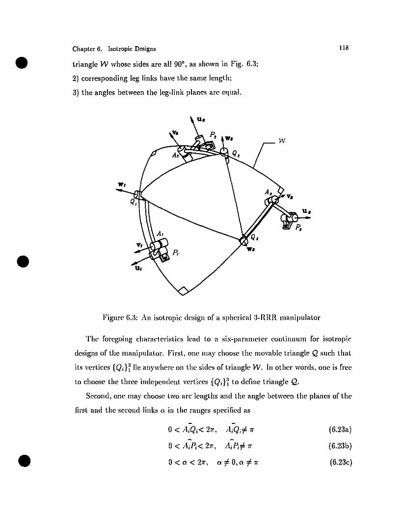
Chapter 6. Isotropie Designs

triangle W whose sides are ail 90°, as shown in Fig. 6.3;

2) corresponding leg links have the sarne length;

3) the angles between the leg-link planes are equal.

Figure (i.:l: An isotropie design of a spherical a-RRR manipulator

118

The foregoing characteristics lead to a six-parameler continuum for isotropie

designs of the manipulator. Firsl, one ma)' choose lhe 1lI0vable triangle 12 such lhal

its verlices {Qin lie an)'where on the sides of triangle W. [n other words, one is free

lo choose the thrcc independent vertices {Qin lo define triangle 12.

Second, one ilia)' choose two arc lengths and lhe angle between the planes of the

first and the second links (\ in the ranges specified as

- -0< AiQi< 27l', t1 i Q47l' (6.23a)

-0< AiPi< 27l', AjP47l' (6.231>)

• 0< 0' < 27l', 0' '" 0,0' '" 7l' (6.23c)

In the case in which we choose three vertices of triangle Q such that it cannot

be inscribed in triangle W, an isotropie design is impossible. That is why Gosselin

(1988) couId not find any. A typical isotropie design of the manipulator is depicted in

Fig. 6.3. Clearly, the set of isotropie designs of the manipulator reported by Gosselin

and Lavoie (1993) is a suhset of the six-dimensional continuum, described above,

which constitutes the complete set of ;sotropic designs for the manipulator at hand.

•Chapter 6. Isotropie Designs 119

•

6.2.4 Spherical DT Manipulator

In this subsection, we find isotropie designs for the spherical DT manipulator, as

shown in Fig. 3.7. It is recalled that a design is isotropie if both J and K are

isotropie, i.e., if eqs.(6.2a) and (6.2b) hold. Equation (6.2a), upon substituting the

value of J of eq.(5.24b) and simplification, yields a diagonal matrix, namely,

(6.24)

o 0 c~

Similarly, eq.(6.2b), upon substituting the value of K of eq.(5.24c) and simplification,

yields

dTd l dTd2 dTd3

dTd27" d"fd = r 21 (6.25)d 2 d 2 2 :1

dTd3 dfda dfd3

where

di == ri x ti, i = 1,2,3

Equations (6.24) and (6.25) lead to the conditions for isotropy, namely,

•(6.26a)

(6.26b)

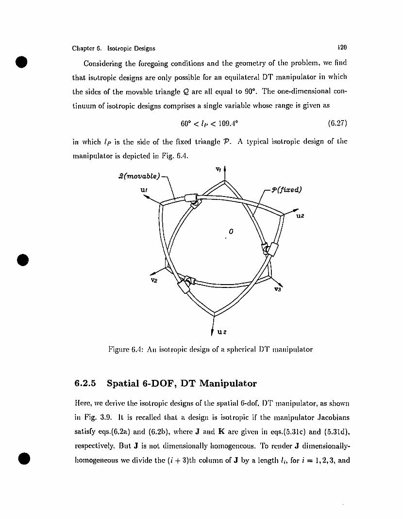
Considering the foregoing conditions and the geometry of the problem, we find

that iS<Jtropie designs are only possible for an equilaterdl DT manipulator in whieh

the sides of the movable triangle Q are ail equal t.o 90°. The one-dimensional con­

tinuum of isotropie designs comprises a single variable whose range is given as

•Chapter 6. Isotropie Designs

60° < lp < 10904°

120

(6.2ï)

•

•

in whieh lp is the side of the fixed triangle 'P. A typieal isotropie design of the

manipulator is depieted in Fig. 604 .

.2(movable)

Ut

V2

U2

Figure 604: An isot.ropie dt'sigll of a spht'rical DT mallipulator

6.2.5 Spatial 6-DOF, DT Manipulator

Bere, we derive the isotropie designs of the spatial (i-dor. DT mauipulator, as shown

in Fig. 3.9. It is reealled that a desigu is isotropie if the manipulator .Jacobians

satisfy eqs.(6.2a) and (6.2b), where J and Karl' given in eqs.(5.31e) and (5.31d),

respeetively. But J is not dimensionally homogeneous. '1'0 rendel· J dimensionally­

homogeneous we divide the (i + 3)th eolumn of J by a length li, for i = 1,2,3, and

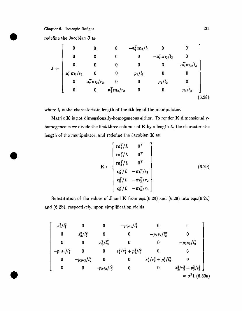
Chapter 6. Isotropie Designs 121

• redefine the Jacobian J as

0 0 0 -afml/ll 0 0

0 0 0 () -aIm 2/12 0

0 0 0 0 0 -aIma/laJ(-

afml/rl 0 0 pt/II 0 0

0 aIm2/1'2 0 0 pdl2 0

0 0 aIma/1'a 0 0 Pa/la(6.28)

where li is the characteristic Iength of the ith leg of the manipulator.

Matrix K is not dimensionally-homogeneous either. To rendcr K dimensionally­

homogeneous we divide the first three columns of K bya Icngth L, the charactcristic

length of the manipulator, and redcfine the Jacobian K as

mT!L OT

• mI/L 0'1'

mI/L OTK(- (6.2!J)

qI/L -mI/1'1

qI!L -mI!1'2

qI/L -m~Fa

Substitution of the values of J and K from eqs.(6.28) and (6.29) into cqs.(6.2a)

and (6.2b), respectively, upon simplification yields

o5~m 0 0 -Plo5lm 0 0

0 o5~m 0 0 -P2052/1~ 0

0 0 052/12 0 0 -Pasa/l~a a

-Plo5l/l~ 0 0 o5~M +p~m 0 0

0 -P2052/1~ 0 0 o5~M+p~m 0

0 0 -pao5a/l"5 0 0 055/1'"5 +p5/1"5• =0-21 (6.30a)

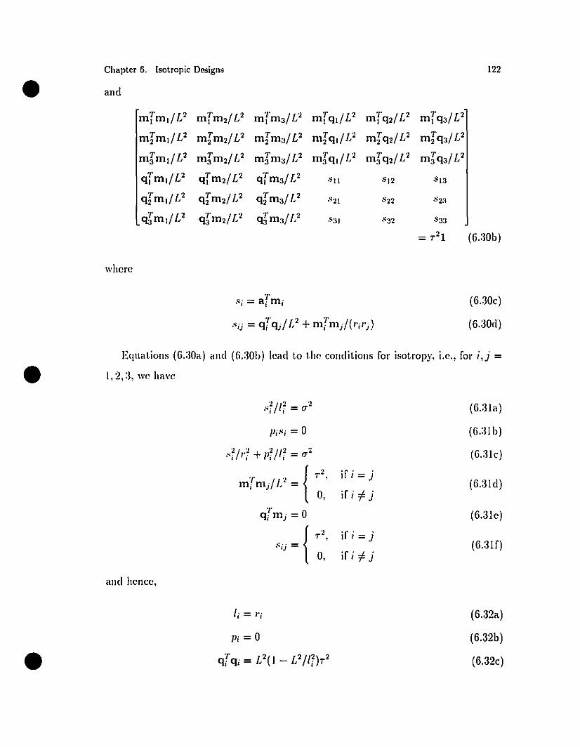
Chapter 6. Isotropie Designs 122

• and

mfml/U mfm 2/ L2 mfm 3/U T /U T /U mfq3/Umtql m 1q2

mIml/U mIm2/U mIm 3/U mIql/U T / 2 mIq3/Um 2q2 L

mImtlU mIm 2/U mIm 3/U T 2 mIq2/ U mIq3/ L2m 3ql/L

qfm l/L2 qfm2/L2 T 2ql m3/ L "'II 05 12 05 13T 2 T / 2 T 2q2 m l/ L q2m2 L q2 m3/ L 821 05 22 ·'523

T 2 qIm 2/U q~m3/UCfJmJ! L .531 ·"32 .533

= T21 (6.:30b)

where

(6.30c)

(6.:30d)

Equations (6.:30a) Hud (G.:30b) lead to the conditions for isotropy, i.e., for i,j =

• 1,2, :1, wc have

2 2 2 (G.3Ia),,;IIi ="

PiSi = 0 (G.:lIb)

,,2/,.2 + p2/l2 =,,2 (6.:31 c)1 1 1 1

2 if i = jT 2 {

T.mim)L = (6.:31 d)

0, if i i' jT (6.:3le)qi mj = 0

sij = {2 if i = jT,

(6.3H)0, if i i' j

and hence,

li = l'i (6.:32a)

Pi = 0 (6.32b)

• qTqi = L2(1_ L2/mT2 (6.32c)

bl = b2 = ba (6.32d)

(CI X mdT(ct X mJl = (C2 X m2f(c2 X m2) = (ca X ma)T(ca X ma)•Chapter 6. Isotropie Designs 123

•

(6.32e)

Moreover, eqs.(6.31a-f), the isotropy conditions, produce manipulators with the fol­

lowing characteristics:

1) The three planes containing veetors ri and bi, for i = 1,2,3, arc orthogonal;

2) the set{riH is orthogonal;

3) the set {biH is orthogonal;

4) ai, for i = 1,2,3, is perpendicular to the plane of veetors ri and bi;

5) the distances between ai and bi, for i = 1,2,3, are equaI.

The foregoing characteristics lead to a one-parameter continuum for isotropie

designs of the manipu!ator. The one-dimensiona! design paramcter l' is defined as

follows:

(6.33)

The continuum of isotropie design is given as

(6.:34 )

•

A typical isotropie design of the manipulator is depicted in Fig. (6.5).

•

•

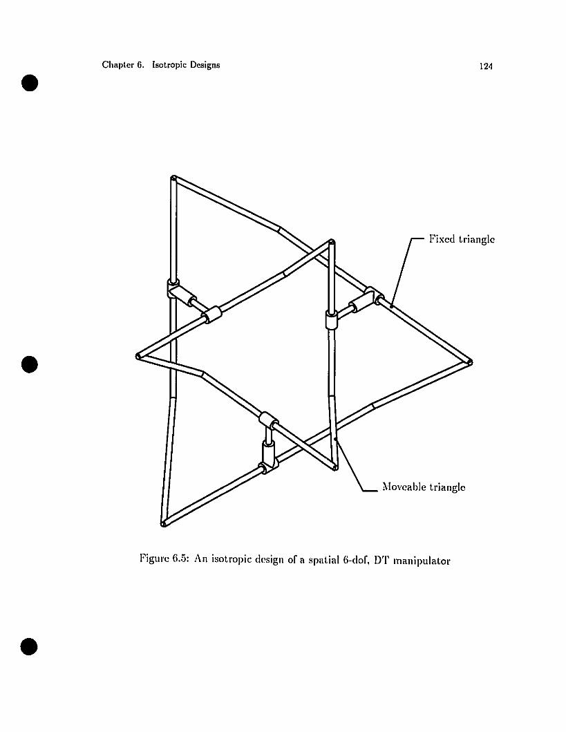
Chaptcr 6. Isotropie Dcsigns 124

Fixed triangle

Moveable triangle

•

FigUl'e fi.5: An isotropie design of a spatial fi-dof, DT manipulator

•

•

•

Chapter 7

Concluding Remarks

1.1 Conclusions

Research interest in parallel manipulators was prompted by the realization that

serial-manipulator performance is deficient. The source of deficiencies in these ma­

Ilipulators is their cantilever type of link loading. Therefore, the obvious alternative

is a parallel architecture, in which the end-effector is supported with a multiple point

support. However, long sIender legs, which are the source of flexibility, are present

in parallel manipulators. A novel class of parallc! device, namc!y, double-triangulaI'

(DT) manipulators, in three versions, was introduced to alleviate this problem. Min­

imum leg lengths occur as a common feature of this new class of manipulators.

Solutions to the direct kinematics (DK) of planaI', spherical and spatial DT ma­

nipulators were attempted and obtained. Using planaI' trigonometry, we found a

quadratic equation solution for the planaI' DT manipulator. The DK of the spherical

DT device was solved, as a 16th order polynomial, by means of spherical trigonom­

etry. These results inductively led us to invoke methods of spatial trigonometry to

treat skew lines. Spatial trigonometric relationships, in turn, were expressed in dual­

number algebra, while the 6 real components of a unit dual vector are the Plücker

coordinates of a line. With the aid of spatial trigonometry, we formulated and solved

the direct kinematic problem of several versions of spatial DT manipulators. These

results revealed that screw operators and the Plücker coordinates of a line expressed

by unit dual quaternions and unit dual vectors, respectively, provide the most efficient

means to formulate, manipulate and solve the kinematics of complicated problems

where motion is constrained by line contact.

A dual 3 x 3 matrix representing a screw motion was derived in an invariant

form. It was shown that the linear invariants of this matrix provide a convenient

way 1.0 compute the screw axis, the angle of rotation and the displacement along the

screw axis of a g'~neral motion. These invariants have bccn traditionally computed

by equation solving, which should be avoided in real-time applications. Therefore,

obtaining these parameters from the linear invariants of the dual matrix reduces the

COmlltltational burden to simple sums and differences.

It is customary to express .Jacobian matrices of parallelmanipulators component­

wise. Indeed, this practice is frequently encountered in the robotics literatUl'e. This

practice leads to equations that are frame-dependent and cumbersome to interpret.

The comp' OIent-wise expressions in such .Jacobian matrices are lengthy and do not

gi\'l' much geometric insight into the belmvionr of the manipula tOI'. As an alternative.

I\'e derived the .Jacobian matrices of certain large classes of parallel manipulators in

an invariant fonn. The .Jacobian matrices found in this way are compact, give direct

geomctric interpretations of the manipula1.01' behavionr, are frame-independent, and

are algebraically simpler. MOl'eover, wc proposed a general method to derive the

.Jacobian matrices of parall,,1 manipnlators al. large. For example. wc unified the

.Jacobian matrices for a large c1ass containing 20 manipula1.01' types into a single

fonnula.

A general classification of singnlarities encountered in parallel manipulators was

introduced and categorized in three singularity types. This classification scheme re­

lies on the conditioning of the Jacobian matrices. Having derived the J acobian matri­

ces in an invariant fonn, allowed us to delect ail singularities within the workspaces

•

•

•

Chaptcr i. Concluding Rcmarks 126

of the manipulators under study. Moreover, we showed that, contrary to earlier

daims, the third type of singularity is not necessarily architecture-dependent.

An important property of robotic manipulators is their dexterity. We regarded

dexterity in the context of local kinetostatic accuracy. Among various measures pro­

posed for quantification of dexterity, we adopted the condition number. This measure

does not share the drawbacks suffered by other measures like the determinant, the

manipulabilityand the minimum singular value. A manipulator design with opti­

mally conditioned Jacobian matrices was called isotl·opic. Having formulated the

Jacobian matrices of the manipulators at hand, in an invariant form, we found the

conditions leading to i~'.ltropic designs. For several manipulators, we were able to find

the complete set of isotroj1ic designs. The isotropie design parameter spaces of these

manipulators turn out to be a continuum of at least one dimension. This provides

a substantial domain of dextrous design choice to fit many situations, which should

admit design criteria other than isotropy, e.g., workspace volume, global dexterity.

•

•

Chapter 7. Concluding Remarks 127

•

7.2 Consideration for Future Work

A few recommended topics for future research are listed below:

1. A polynomial of degree 16 wa.~ found for the direct kinematic problem of spher­

ical DT manipulator. The result implies that the polynomial ha.~ at most 16

solutions, among which only eight would be real positive. Since only the real

positive solutions are acceptable, the direct kinematic problem of this device

has at most eight solutions. However, in tests we ran, we could find no instance

with more than t.wo geometrically distinct solutions. Therefore, the polynomial

is not minimal. Finding the minimal polynomial would be a topic of further

research.

2. The direct kinematic problem of ail versions of spatial DT manipulators was

formulated in this thesis, without dosed form solutions. This issue remains as

•Chapter 7. Concluding Remarks

a challenging research problem.

128

•

•

3. It has been shown that dual quaternion algebra is an excellent tool to handle

the kinematics of line-contact constrained mechanisms. The kinematic study

of other mechanisms of this type, such as the double-tetrahedral mechanism,

by this means, constitutes another possible extension to our wurk.

4. The main rcason why dual numbers, quaternions and dual quaternions are not

popular is that they are difficult to work with. To overcome this obstacle the

author implemented sorne user-defined functions in MATHEMATICA to han­

dIe sorne dual number algebraic operators. It is suggested that a computational

algebraic code be devcloped to make these computations as convenient as those

currently available for complex, vector and matrix algebras.

5. It was shown that expressing the Jacobian matrices in an invariant form makes

it easier to effectivc1y handle the issues of isotropy and singularity. Another

challenging and fruitful problem is to find the continuum of isotropic designs

and singular configurations of the most common parallel manipulator, i.e., the

Stewart-Gough platfonn, \Vith invariant forll1s of its Jacobian matrices.

6. Multi-parameter continua of isotropic designs for some manipulators were found.

This allo\Vs one to incorporate desig!l criteria other than isotropy. Clearly, de­

signing manipulators with ll1ulti-variate objective functions, including isotropy,

is a topic worthy of further research .

•

•

•

References

Agrawal, O. P., 1987, "Hamilton Operators and Dual-Number-Quaternions in Spatial

1<inematics," Mechanism and Machine Theory, Vol. 22, No. 6, pp. .569-.57.5.

Albala, H., 1982, "Displacement Analysis of the General n-Bar, Single-Loop, Spatial

Linkage, Part 1: Underlying Mathematics and Useful Tables. Part Il: Basic f)is­

placement Equations in Matrix and Algebraic Form," J. Mechanical Design, TI'IIIlB.

ASME, Vol. 104, No. 2, pp. 504-525.

Alizade, R., Duffy, J. and Hatiyev, E. 'l'., 1983, "Mathematical Modcls for Analy­

sis and Synthesis of Spatial Mechanisms, I-IV," Mec!ulIlism mlll Il'iachinc Thcol'Y,

Vol. 18, No. 5, pp. 301-328.

Angeles, J., 1988, Ralionalli'inCllwtics, Springer-Verlag, New York.

Angeles, J., Anderson, 1<., Cyril, X. and Chen, 8., 1988, "The Kincmatic Invcrsion

of Robot Manipulators in the Presence of Singularitics," ASME J. of Mcc!ulflisms,

Transmissions, and Automation in Design, Vol. 110, pp. 246-254.

Angeles, .1., Hommel, G. and Kovacs, P., 1993, Computational liïnematics, 1<luwcr

Academie Publishers, Dordrecht.

Angeles, J. and Lôpez-Cajtin, C. S., 1992, "1<inematic Isotropy and the Conditioning

Index of Seriai Robotic Manipulators," The /nt. J. Robotics Research, Vol. Il, No. 6,

pp. 560-570.

Angeles, J., Ranjbaran and Patel, R. V., 1992, "On the Design of the Kinematic

Structure of Seven Axes Redundant Manipulators for Maximum Conditioning," Pme.

IEEE In/. Conf. on Robo/ies A Il/oma/ion, Nice, Vol. I. pp. 494-499.

•References 130

•

•

Bpll, Sir P.. S., 1900, The TheO/'Y of S'erelVs, Cambridge University Press, Cambridge.

Behi, F., Mehregany, M. and Gabriel, K., 1990, "A Microfabricated Three-Degree­

of-Freedom Parallel mechanism," Pme. IEEE Miem E/ec/m Mecllflnieal S'ys/ems:

An lnvesligalion of Micro S'iruc/ures, Sensors. Aelualors. 1\laehine.~ and Robols.

pp. 159-165

Charentus, S. and Renaud, M., HJ89, Calcul du modèle géomélrique direc/e ,le

la plaie-forme ,le S'lelllarl, LAAS Heport # 89260. Laboratoire d'Automatique ct

d'Analyse de Systèmes, Toulousc.

Chellg, Il. Il., Hm:!, "Compulatiolls of Dual !\umbcrs ill the Extended Finite Dual

Plallc" l'me. IISMH COllf. 011 AdlHlI/ccs ill Design Aulomalioll, Albuquerque. Vol. 2.

pp. ;:1-80.

Clavel, Il., I!J88, "DEr;rA, a Fast Hobot with Parallel Gcometry:' Pme. 1111. Sym­

posium fJ/l Ir"luslrial Robols. Lallsannc. pp. !Jl-IOO.

Clifrord, W. 1\.. 18n. "Prelilllinary Sketch of Bi-Quatel'llions." Proe. LOlldon Mfllh.

S'oc.. Vol. '1. pp. :181 <Ilm.

Cox, D..1. and 'l'csar, n., I!l8!J. "Thc Dynamic j'l'Iodcl or a Three-Degree-of-Freedom

Parallel Robotic Shoulder Module:' Pme. Forth Inl. COllf. 011 Advalleed Robolies,

Columbus, Ohio.

Craver, W. i"l., 1989, "Structmal Analysis and Design of a Three-Degrec-of-Freedom

Robotic Shoulder Module," M. Ellg. Thesis, The Universily of Texas at Allstill,

A IlSIiIl.

Duffy, J. and Crane, C., 1980, "A Displacement Analysis of the General Spatial 7­

Link, 7R Mechanism," Mcchanism and Machinc ThcO/'y, Vol. 15, No. 3, pp. 153-159.•References 131

•

•

Duffy, J. and Derby, S.. 1979, "Displacement Analysis of a Spatial 7R Mechanism: A

Generalized Lobster's Arm," J. Mcchanical Dcsigll, Trans. ASME, Vol. 101, No. 2,

pp. 224-231.

Funda, J. and Paul, R. P., 1990, "A Computational Analysis of Screw Transfor­

mations in Robotics," IEEE Trans. on Robolics and Aulomalion, Vol. 6, No. a,pp. 348-356.

Ge, J. Q., 1994, "On the Matrix Algebra Realization of the Theory of Biquaternions,"

Proc. ASME Conf. on Mcchanism Synlhcsis and Analysis, Minnesota, pp. 425-432.

Ge, J. Q. and McCarthy, J. M., 1991, "Functional Constraints as Aigebraic Manifolds

in a Clifford Algebra," IEEE 11·ans. on Robolics And Aulomaliofl, Vol. 7, No. 5,

pp. 670-677.

Gonzalez-Palacios, M. A. and Angeles, J., 1993, Cam SY'llhcsis, I\luwer Academie

Publishers, Dordrecht.

Gosselin, C., 1988, "Kinematic Analysis, Optimization and Programming of Parallel

Robotic Mani]>ulators," Docl01'll1 Dissc7'lalion, McGill Univc7'sily, Monll'cal, Qllcbcc.

Gosselin, C. and Angeles, J., 1988, "The Optimum Kinematic Design of PlanaI'

Three-Degree-of-Freedom Parallel Mani]>ulator," ASME J. of Mcc/wnism.$, 1hms­

missions, ami Aulomalion in Dcsign, Vol. 110, No. l, ]>]>.15-41.

Gosselin, C. and Angeles, J., 1989, "The Optimum Kinematic Design of Spherical

Three-Degree-of-Freedom Parallel Manipulator," ASME J. of Mcc/wnisms, Tmns­

missions, and Aulomation in Dcsi!in, Vol. 111, No. 2, pp. 202-207.

Gosselin, C. and Angeles, J., 1990a. ·'Kinematic Inversion of Parallel Manipulator in

the Presence of Incompletely Specified Tasks,~ .J. Jl1ecllllllica/ Design, Trans. ASME,

Vol. 112, pp. 494-.500.•Rcrcrcnccs 132

•

•

Gosselin, C. and Angeles, .J., 1990b, "Singlliarity Analysis of Closed-Loop I\inematic

Chains," IEEE Trans. on Robolies and Aulomalion, Vol. 6, No. 3, pp. 281-290.

Gosselin, C. M. and Hamel, .J.-F., 1993, "The Agile Eye: a High-Performancc Three­

Degree-of-Freedom Camera-Orienting deviee," Rapporl Technique, Déplll'lemeni de

Génie Jl1éellnique, Université LavII/.

Gosselin, C. M. and Lavoie, E., 1993, "On the Kinematic Design of Spherical TIIree­

Degree-of-Freedom Parallel Maniplliators," The Inl . .J. Robolics Re.<ellreh, Vol. 12,

No. 4, pp. 394-402.

Gosselin, C. M. and Sefriolli, .J., 1991. "Polynomial Solutions for the Direct Kine­

matie Problcm of PlanaI' Three-Degree-of-Freedom Parallel Maniplliators," Proe.

Fiflh 1,,1. Conf. 011 Ad'll/nercl Robolie". Pisa. pp. 1124-1129.

Gosselin, C. M., Sefrioui. .J., and Hichard, M. .J., 19~J;la. "On the direct kinematies of

spherical three-degree-of-freedolll parallel manipulators with a coplanar platform",

ASME.J. Mechll"icII/ Dc,5ig". Vol. 116, pp. 58ï-59:3.

Gosselin, C. M., Sefrioui . .J., and Hichard. M. J., 19~J;lb. "On the direct kinematics

of sphel'ical three-dcgrec-of-frecdom parallel manipulators of general architecture".

ASME .J. Mec/Ill/liea/ Design, Vol. 1Hi, pp. 5!J'1-598.

Gupta, 1\. C. and Hoth, B., 1!J82, "Design Considerations fol' i\laniplllatol' \Vorkspace,"

ASME.J. of Mec/ul1Iisms Desigll, Vol. 104, No. 4, pp. ï04-ïI2.

Hamilton, W. A., 1844, "On Qllate1'l1ions: 01' a New System of Imaginaries in Alge­

bra," Phil. l'l'!lIg. 3rd Sel'. 25, pp. 489-495.

Hara, A. and Sugimoto, 1\., 1989, "Synthesis of parallel micl'Omaniplliators," Trans .

• References

of the ASME, Vol. Hl, pp. 34-39.

133

•

•

Hayward, V. and Kurtz, R., 1991, "Modeling of a Parallel Wrist Mechanism With

Actuator Redundancy," in Stifter, S. and Lenareic, J. (editors) Advance in Robot

Kinematics, Springer Verlag, pp. 444-456.

Hervé, J. M. and Sparaeino, F., 1991, "Structural Synthesis of 'Parallel' Robots

Generating Spatial Translations," Proc. Fifth Int. Conf. on Advanced Robotics, Pisa,

pp. 808-813.

Householder, A. S., 1970, The Numerical Treatment of a Single Nonlinear Equation,

McGraw-Hill Book Company.

Hunt, K. H., 1983, "Structural Kinematics of In-Parallel-Actuated Robot Arms,"

ASME J. of Mechanisms, Transmissions, and Automation in Design, Vol. 105, No. 4,

pp. 705-712.

Hunt, K. H., 1986, "Special Configurations of Robot-Arms Via Screw Theory, Part

l," Robotica, Vol. 4, pp. 171-179.

Hunt, K. H., 1987, "Special Configurations of Robot-Arms Via Screw Themy, Part

2," Robotica, Vol. 5, pp. 17-22.

Hunter, 1. W., Lafont~ine, S., Nielsen, P. M. F., Hunter, P. J. and Hollerbach, J. M.,

1989, "Manipulation and Dynamic Mechanical Testing of Microscopie Objects Using

a Tele-Micro-Robot System," Proc. IEEE Int. Conf. on Robotics and Automation,

Scottsdale, pp. 1553-1557.

Husty, M. L., 1994, "An Algorithm for Solving the Direct Kinematic of Stewart­

Gough-Type Platforms," Department of Mechanical Engineering & Centre for Intel­

ligent Machines Technical Report, McGill University, Montreal.

Busty, M. L. and Zsombor-Murray, P..1.,1994, "A Special Type of Singular Stewart­

Gough Platform, in Lenarëië, .1. and Ravani, B. (editors) Advanec.$ in Robol liÏnc­

malies and Compulalional Gcomcll'Y, Kluwer Academic Publishers, pp. 449-4.58.

•References 134

•

•

I-Iusty, M. L. and Angeles, .1., 1994, "Kinematic Isotropy in 3R Positioning Manipu­

lators," in Lenarëië, .1. and Ravani, B. (editors) Advanccs in Robol Kincmalies and

Compulalional Gcomcll'Y, Kluwer Academic Publishers, pp. 181-190.

IFToMM Commission A on Standards for Terminology, 1991. "Terrninology for the

Theory of Machines and MechanisI1ls," Mechanisl/l and Machine Theol',I', Vol. 26,

No..5, pp. 435-.539.

Issacson, E. and Keller, II. B., 1966, Arwlysis of NUlllcl'ical Mclhot/s, New York,

Wiley.

Klein, C. A. and Blaho, B. E., I!J8i, "Dexterity Measures for the Design and Control

of Kinematically Redundant Manipulators." Thc 1111. J. Robolies Rcscareh. Vol. 6,

No. 2, pp. i2-83.

Klein, C. A. and Miklos, T. A.. 1991, "Spatial Robotic Isotropy," The Inl. J. Robolies

RCSClll'ch, Vol. 10, No. 4, pp. '126-43i.

Lai, Z. C. and Yang, D. C. H., 1986, "A New Method fol' the Singularity Analysis

of Simple Six-Link Manipulators," The Inl. J. Robolies Rcscarch, Vol. 5, No. 2,

pp. 66-i4.

Lee, 1-1. Y. and Liang, C. G., 1988, "Displacement Analysis of the General Spa­

tial Seven-Link iR Mechanism," MecililnisllJ and Machine Theory, Vol. 23, No. 3,

pp. 219-226.

Lee, K. M. and Yien, C., 1989, "Design and Control of a Prototype Platform Manip­

ulatol' fol' Workhandling Applications," J. Mcehallical IVorking Teehnology, Vol. 20,

pp. 305-314.

Lee, H., Woernle, C. and Hiller, M., 1991, "A complete solution for the inverse

kinematic problem of the general 6R robot manipulator," J. Mechanical Design,

Trans. ASME, Vol. 113, pp. 481-486.

• References 135

•

•

Liégeois, A., 1977, "Automatic Supervisory Control of the Configuration and Be­

havior of Multibody Mechanisms," IEEE Trans. Sys. Man Cybernet., SMC-Vol. 7,

No. 12, pp. 868-871

Litvin, F. L. and Parenti-Castelli, V. , 1985, " Configurations of Robot's Manipu­

lators and Theil' Identification, and the Execution of Prescribed Trajeetories, Part

1: Basic Concepts," ASME J. of Mechanisms, Transmissions, and Automation in

Design, Vol. 107, pp. 170-178.

Litvin, F. L., Yi, Z., Parenti-Castelli, V. and Innocenti, C., 1986, " Singu!arities,

Configurations, and Displacemen'. Functions for Manipulators," The Int. J. Robotics

Resea7'ch, Vol. 5, No. 2, pp. 52-65.

Ma, O., Angeles, J., 1992, "Architecture Singularities of Parallel Manipulators," The

Int. J. of Robotics and Automation, Vol. 7, No. 1, pp. 23-29.

Merlet, .J.-P., 1989, "Manipulateurs parallèles, 4ième partie: Modes d'assemblage et

cinématique directe sous forme Polynomiale," Technical report, INRIA, France.

Merlet, J.-P., 1990, Les Robots Parallèles, Hermès Publishers, Paris.

Mohamed, M. G., 1983, "Instantaneous Kinematics and Joint Displacement Analy­

sis of Fully-Parallel Robotic Devices," Doctoral Dissertation, Unive7'sity of Florida,

Florida.

Mohammadi Daniali, H. R. and Zsombor-Murray, P. J., 1994, "The Design oflsotropic

PlanaI' Parallel Manipulators," in Jamshidi, M., Yuh, J., Nguyen, C. C. and Lumia,

R. (editors) Intelligent Automation and Soft Computing, TSI press, Vol. 2, pp. 273­

280.

Mohammadi Daniali, H. R., Zsombor-Murray, P. J. and Angeles, J., 1993a, "On

Singularities of PlanaI' Parallel Manipulators," Proe. ASME Conf. on Design Au­

tomation, Albuquerque, pp. 593-599.

• References 136

•

•

Mohammadi Daniali, II. R., Zsombor-Murray, P. J. and Angeles, J., 1993b, "The

Kinematics of 3-Dof PlanaI' and Spherical Double-TriangulaI' Parallel Manipulators,"

in Angeles, J., I-Iommel, G. and Kovacs, P. (editors) Computational Kinr.maties,

Kluwer Academie Publishers, Dordrecht, pp. Ui3-164.

Mohammadi Daniali, H. R., Zsombor-Murray, P. J. and Angeles, J., 1994a, "Isotropie

Design of Spherica! Paralle: Manipulators," Proe. ASME Conf. on Design Automa­

tion, Minnesota, pp. 461-466.

Mohammadi Daniali, H. R., Zsombor-Murray, P. J. and Angeles, .L, 1994b, "Sin­

gularity Analys;s of Spherical Parallel Manipulators," The Tenth CISill-IFToMkI

Symposium on the Theory and Pl'lleticc of Robo/ie Marlipulators, Gdansk, in press.

Mohammadi Daniali, H. R., Zsombor-Murray, P. J. and Angeles, J., 1994c, "The

Design of Isotropie PlanaI' and Spherica! Parallel Manipulators," Robotie Meeha'lieal

Systems Gmdull/e Studen/s Forum, lHcGill University, Mon/real, June 27-29.

Mohammadi Daniali, H. R., Zsombor-Murray, P..1. and .\ ngeles, J., 1994d, "The

Kinematics of Spatial Double-TriangulaI' Parallel Manipulators," /0 appear in J.

klee/ulIlical Design, Tmns. ASME.

Mohamm~di Daniali, H. R., Zsombor-lVlurray, P. J. and Angeles, J., 1995a "Singu­

larity Analysis of PlanaI' Parallel Manipulators," Meehanism and Machine Them'y,

Vol. 30, No. $, pp. 665-678.

Mohammadi Daniali, 1-1. R., Zsombor-Murray, l'. J. and Angeles, J., 1995b, "Singu­

larity Analysis of a General Class of PlanaI' Parallel Manipulators," ta be presented

at 1995 IEEE Int. Conf. on Roboties and Automation, Nagoya, Japan.

Mohammadi Daniali, H. R., Zsombor-Murray, P. J. and Angeles, J., 1995c, "Direct

Kinematics of Double-Triangular Parallel Manipulators," to appear in Mathematiea

Pannoniea.

• References 137

•

•

Mohammadi Daniali, H. R., Zsombor-Murray, P. J. and Angeles, J., 1995d, "The

Isotropie Designs of Two General Classes of Planar Parallel Manipulators," to appear

in J. of Robotie Systems.

Nanua, P., Waldron, 1<. J. and Murthy, V., 1990, "Direct Kinematic Solution of a

Stewart Platform," IEEE Trans. on Roboties and Automation, Vol. 6, No. 3, pp. 438­

444.

Nguyen, C. G. and Pooran, F. J., 1989, "KinematicAnalysis and Workspace Determi­

nation of a 6 Dof CKCM Robot End-Effector," J. ofMeehanieal Working Teehnology,

Vol. 20, pp. 283-294.

Notash, L. and Podhorodeski, R. P., 1994, "Uncertainty Configurations of Three­

Branel! Parallel Manipulators: Identification and Elimination," Proe. ASME Conf.

on Roboties: /(inematics, Dynamies and Controls, Minnesota, pp. 459-466.

Ogino, S. and Watanabe, 1<., 1969, "Study on Spatial Four-Link Chain Having Four

Cylindrical Pairs," Bulletin of the Japan Society of Meehanieal Engineering, Vol. 12,

No. 49, pp. 97-113.

Paul, R. P. and Stevenson, C. N., 1983, "Kinematics of Robot Wrists," The Int. J.

Roboties Research, Vol. 2, No. 1, pp. 31-38.

Pieper, D. L., 1968, The Kinematics of Manipulators under Computer Control, Ph.

D. Thesis, Stanford University, Stanford, CA.

Pierrot, F., Fournier, A. and Dauchez, P., 1991, "Towards a Fully-Parallel 6 DOF

Robot for High-Speed Applications," Proe. IEEE Int. Conf. on Robotics and Au­

tomation, Sacramento, pp. 1288-1293.

Pittens, K. H. and Podhorodeski, R. P., 1993, "A Family of Stewart Platforms with

Optimal Dexterity," J. Robotics and Autonomous Systems, pp. 463-479.• References 138

•

•

Pradeep, A. K., Yoder, P. J. and Mukundan, R., 1989, "On the Use of Dual-Matrix

Exponentials in Robotics Kinematics," The fnt. J. Robotics Research, Vol. 8, No. 5,

pp. 57-66.

Primrose, E. J. F., 1986, "On the Input-Output Equation of the General 7R Mech­

anism," MeC!'~nism and Machine Theory, Vol. 21, No. 6, pp. 509-.510.

Raghavan, M. and Roth, B., 1990, "Kinematic Analysis of the 6R Manipulator of

General Geometry," in Miura, H. and Arimoto, S. (editors), Proc. Fifth fnt. Sympo­

sium on Robotics Resea7'ch, MIT Press, Cambridge.

Raghavan, M., 1993, "The Stewart Platform of General Geometry Has 40 Config­

urations," J. of lV!echanicrt/ Design, Trans. ASME, Vol. 115, No. 1, pp. 277-282.

Salisbury, .1. K. and Craig, J. J., 1982, "Articulated Hands: Force Control and

Kinematic Issues," The fnt. J. Robotics Research, Vol. 1, No. 1, pp. 4-17.

Salmon, G., 1964, Lessons fntror/uctory to the lilor/em Higher Algebra (5th ed.), New

York: Chelsea.

Sefrioui, .1., 1992, "Problème Géométrique Direct et Lieux de Singularité des Manip­

ulateurs Parailèles," Doctoral Dissertation, Université Laval, Québ~c.

Shamir, T., 1990, "The Singularities of Redundant Robot Arms," The fnt. J. Robotics

Resea1'ch, Vol. 9, No. 1, pp. 113-121.

Stewart, D., 1965, "A Platform with Six Degrees of FreedolTt," Mechanism and Ma­

chine The07'y, Vol. 21, No. 5, pp. 365-373.

Study, E., 1903, Geometrie r/er Dynamen, Leipzig, Germany.

Sugimoto, K., Duffy, J. and Hunt, K. H., 1982, "Special Configurations of Spatial

Mechanisms and Robot Arms," Mechanism and Machine Theory, Vol. 17, No. 2,

pp. 11!?·-132.

• References 139

•

•

Suh, K. and Hollerbach, J., 1987, "Local Versus Global Torque Optimization of

Redundant Manipulators," Proc. lnt. Conf. on Robotics Automation, Raleigh, North

Carolina, pp. 619-624.

Tandirci, M., Angeles, J. and Ranjbaran, F., 1992, "The Characteristic Point and

the Characteristic Length of Robotic Manipulators," ASME Biennial M·chanisms

Conference, Vol. 45, pp. 203-208.

Tarnai, T. and Makai, E., 1988, "Physically Inadmissible Motions of a Pair of Tetra­

hedra," Proc. Third lnt. Conf. Eng. Graph. and Desc. Geom., Vienna, Vol. 2,

pp. 264-271.

Tarnai, T. and Makai, E., 1989a, "A Movable Pair of Tetrahedra," Proc. R. Soc.

Land., Vol. A423, 423-442.

Tarnai, T. and Makai, E., 1989b, "I(inematical Indeterminacy of a Pair of Tetra­

hedral Frames," Acta Technica Acad. Sci. Hung., Vol. 102, No. 1-2, pp. 123-145.

Thompson, S. and Cheng, H. H., 1994, "A Dual Iterative Method for Displacement

Analysis of Spatial Mechanisms," Proc. ASME Conf. on Mechanism Synthesis and

Analysis, Minnesota, pp. 23-28.

Yang, A. T., 1963, "Application of Quaternion Algebra and Dual Numbers to the

Analysis of Spatial Mechanisms," Doctoral Dissertation, Columbia University, New

York, No. 64-2803 (University Microfilm, Ann Arbor, Michigan).

Yang, A. T. and Freudenstein, F., 1964, "Application of Dual-Number Quaternion

Algebra to the Analysis of Spatial Mechanisms," J. of Applied Mechanics, pp. 300­

308.

Yoshikawa, T., 1985, "Dynamic Manipulability of Robot Manipulators," The Int. J.

Robotics Research, Vol. 5, No. 2, pp. 99-111.•References 140

•

•

Zlatanov, D., Fenton, R. G. and Benhabib, B., 1994a, "Singularity Analysis of Mech­

anisms and Robots Via a Motion-Space Model of the instantaneous Kinematics,"

Proc. IEEE Int. Conf. on Robotics and Automation, San Diego, pp. 980-985.

Zlatanov, D., Fenton, R. G. and Benhabib, B., 1994b, "Singularity Analysis of Mech­

anisms and Robots Via a Velocity-Equation Model of the instantaneous Kinematirs,"

Proc. IEEE Int. Conf. on Robotics and Autornation, San Diego, pp. 986-991.

Zsombor-Murray, P..1. and Hyder, A., 1992, "An Equilateral Tetrahedral Mecha­

nism," J. Robolics and Autonomous Systems, pp. 22ï-236.

•

•

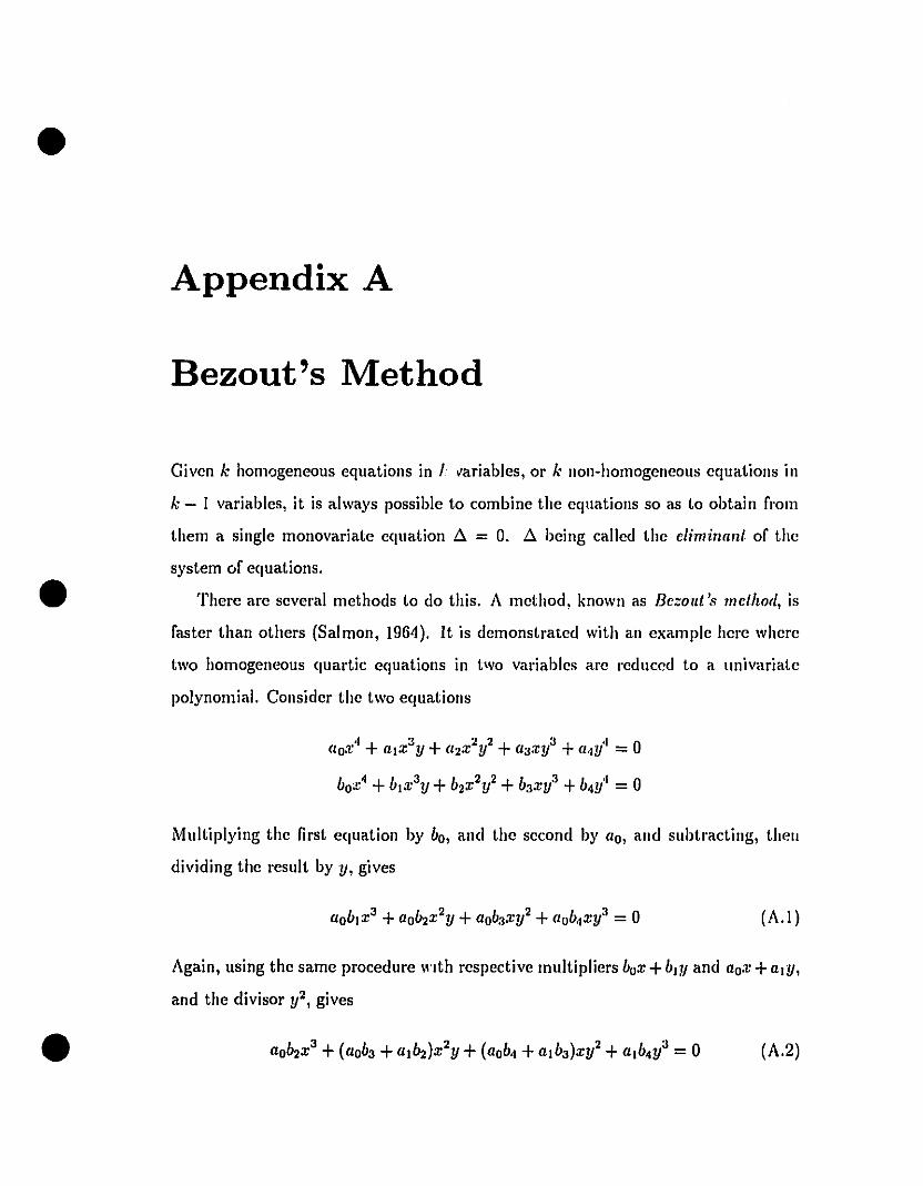
Appendix A

Bezout's Method

Givcn k homogeneous equations in r ~ariables, or k non-homogcneous cquations in

k - 1 variables, it is always possible to combinc the cql1ations so as to obtain from

them a single monovariate equation ~ = O. ~ being called the eliminant of the

system of equations.

There are scveral methods to do this. A mcthod, known as Bezout 's melhotl, is

faster than others (Salmon, 1964). It is demonstrated with an example here where

two homogeneol1s quartic eql1ations in t'Vo variables are redl1ced to a lInivariate

polynomial. Consider the two equations

UoX" + (lIx3y + {I2x2y2 +U3.-c y3 +{l'IY'' =0

box" +b,x3y +b2X2y2 +b3Xy3 +b..y·' = 0

Multiplying the first eql1ation by bo, and the second by {la, and sl1btracting, thell

dividing the result by y, gives

(A.I )

•Again, using the same procedure II"lth respective multipliers box +bly and uox +{l,Y,

and the divisor y2, gives

(A.2)

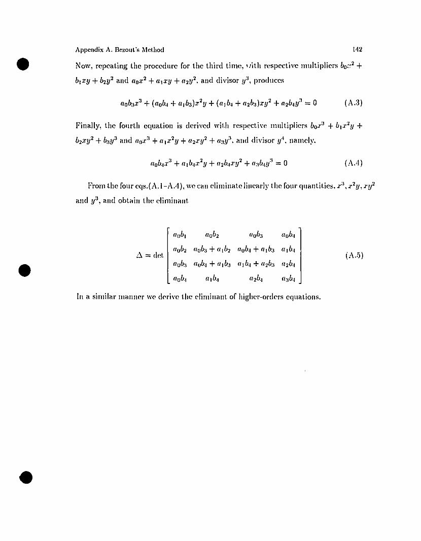
Now, repeating the procedure for the thinl time, 'Jith respective multipliers bo.~,2 +b,xy +b2y2 aud (lo.r2 +(I,xy + (l 2y2. and divisaI' y'l, prodllces•Appendix A. Bezollt's Melhod 142

(:U)

Finally, the fonrth equation is derived with respective multipliers box'l + b,.r2y +

b2.ry2+ b'l1l and lIo;ra + (I,.r2y + (l2.ry2 +(1:1.'/' and divisaI' 1/'. namely,

(AA)

From the four cqs.( A.I-A JI), we cali e1iminate lillcarly the four quantities, x", J.2 y, J'y2

and y'l, and obtaill thc c1iminant.

lIob, 1I0 b2 lIob" Il ob"

D. = deI.1I0 b2 lIob" + Il, b2 lIob., + (l, b'l "l b.1

(A.5)

• (lob" (lob., + Il, b" Il, b.1 + (l2b'l 112 b.,

(lob., (II b'l 112b'l (l'lb.,

III a similar manncr wc dcrÏ\'e the di minant of higher-ol'dcrs cquations.

•

•

•

•

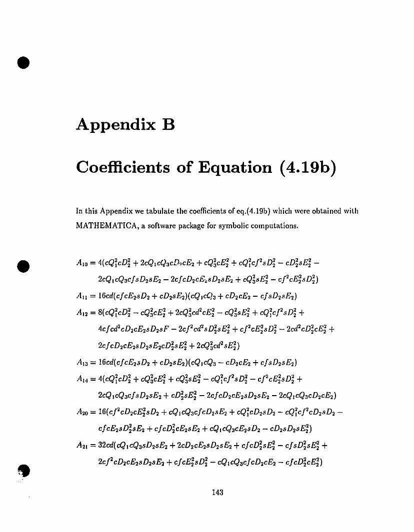
Appendix B

Coefficients of Equation (4.19b)

In this Appendix we tabulate the coefficients of eq.(4.19b) which wcre obtailled with

MATHEMATICA, a software package for symbolic computations.

A IO =4(cQ~cD~ +2CQICQ3CD.cE2 +cQâcE; +cQ~crsD~ - cD;sB; ­

2CQICQ3CjsD2sE2 - 2cJcD2cE,sD2sE2 +cQâsB~ - cJ2cE;sD~)

Ail = 16cd(cJcE2sD2+cD2sE2)(cQlc'h +cD2cE2 - cJsD2sE2)

AI2 = S(cQ~cD; - cQâcE~ +2cQâcd2cB; - cQâsB; +cQ~cJ2sD~ +4cJcd2cD2cE2sD2sF - 2CJ2cd2SD~sE; +crcE;sD~ - 2cd2CD~cE; +

2cJcD2CB2SD2SB2CD~sE~ +2eQâcd2sE;)

A I3 = 16cd(cJcE2sD2+cD2sE2)(cQICQ3 - cD2cB2 +cJsD2sE2)

Al" =4(cQ~cD~ +cQâcE; +cQâsE; - cQ~cJ2sD~ - cJ2cB;sD; +2CQICQ3CJsD2sE2 + cD~sE~ - 2cJcD2cE2sD2sE2 - 2CQICQ3CD2cB2)

A20 = 16(cj2cD2cE;sD2+CQICQ3CJcD2sE2 +CQ~CD2SD2 - cQ~CrCD2.sD2 ­

CJCE2SD~sE2 +cjcDicE2sE2+CQICQ3CE2sD2 - cD2sD2sEn

A2l =32cd(eQICQ3SD2SE2 +2cD2cE2sD2sE2+cJcD~sE~ - cJsD~sE~ +2cj2cD2cE2sD2sE2+cjcE;sD~ - CQICQ3CJcD2cE2 - cJcD~cE~)

143

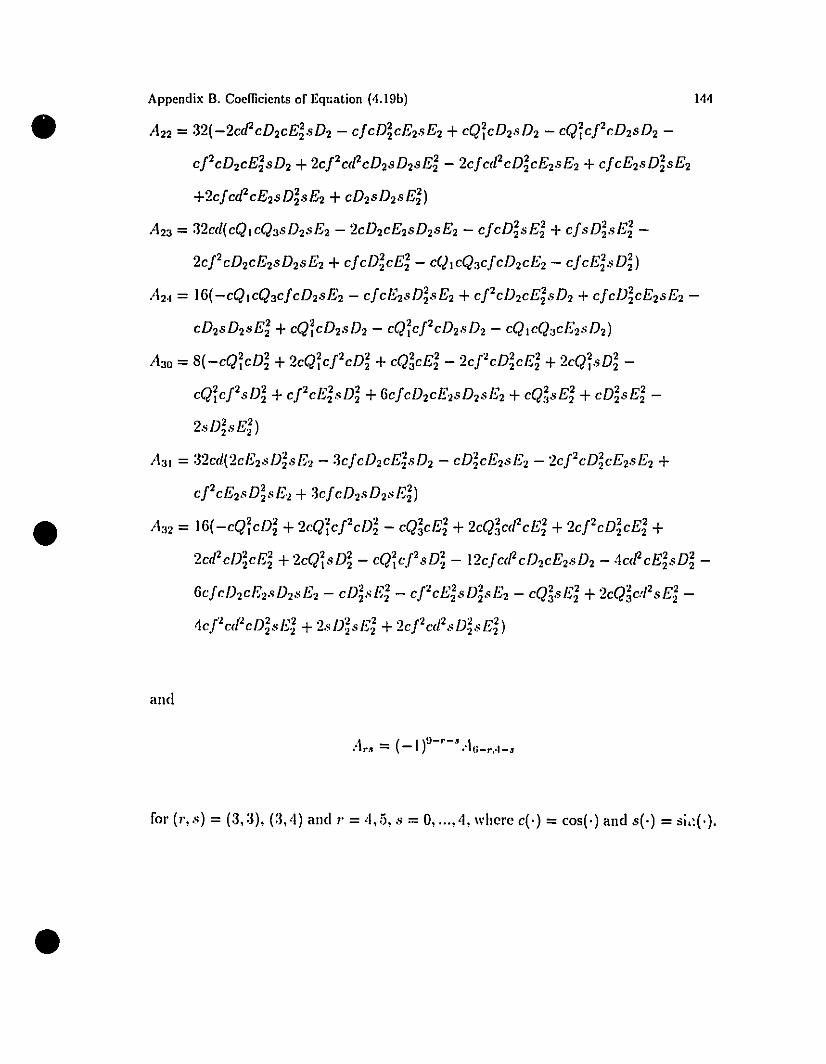
A22 = 32( -2ccfcD2CE~sD2 - cJcD~cE2.sE2 + cQ;cD2sD2 - cQ;cJ2cD2sD2 ­

cJ2cD2cEisD2+2CJ2Cd2CD2SD2SE~ - 2cJcd2cD~cE2SE2 +CJCE2SD~sE2

+2cJcd2CE2SD~sE2 + cD2sD2sEi)

An = 32cd(cQICQ3SJJ2sE2 - 2cD2cE2sD2sE2 - cJcD~sE~ + cJsJJ~.sE~ ­

2cFcD2cE2sD2sE2+ cJcD~cE~ - CQICQ3CJcD2cE2 - cJcEisD~)

Ihl = 16(-cQlcQ3cJcD2sE2 - CJCE2SD~sE2 + CJ2cJJ2CE~sD2 +cJcD~cE2SE2­

cD2sD2sEi +cQ;cD2sD2 - cQ;cJ2cD28D2 - CQICQ3CE2SD2)

A3a = 8( -cQ;cDi +2cQ;cJ2cD~ +cQ~cEi - 2CJ2cD~cE~ +2CQ;.5D~ ­

CQ;CJ2sJJ~ +cJ2cE~sD~ +6cJcD2cE2.5D2.sE2+cQ~sE~ +cD~sE~ ­

?cD2c!"2)...." 2'::>..12

•Appendix B. Coefficients of Eqt:ation (4.19b) 144

•

•

A31 = 32cd(2cE2sD~.5E2 - 3cJcl)2CE~.5D2 - cD~cE2SE2 - 2CJ2CD~cE2.5E2 +

cJ2cE2SD~sE2 + 3cJcD2SD2SE~)

A:12 = 16(-cQ;cD~ +2cQ;CJ2CD~ - cQ~cE~ + 2cQ~cd2CEi +2CJ2CD~cEi +

2c(PcD~cE~ +2cQ;sJJ~ - CQ;CJ2sD~ - 12cJc(PCJJ2CE2sD2 - 4c(PcE~sD~ ­

6cJcD2cE2sJJ205E2 - cD~.Œi - cFcEisD~.sE2 - cQ~s/~i +2cQ~c!PsEi ­

4clc(PcD~o5Ei + 2.5D~8Ei +2cJ2C(PÛ)~sEi)

and

for (1',05) = (3,a), (:3,4) and l' = 4,5, s = 0, ... ,4, whcrc c(·) = cos(·) and s(·) = si,:(·).

•

•

•

Appendix C

Coefficients of Equation (4.38 ~

Here we tabulate qi, for i = l,'" ,8, of eq.(4.38)which were obtained with MATHE­

MATICA, a software package for symbolic computations.

ql = 0.1589146384409058 cos .,pl +0.284268244827663 sin !/J3

-0.6356385402223707 sin !/J3 sin.,pl - 0.4264022119870481 sin !/J2

q2 = -0.402014~020702365 cos !/J3 - 0.6356385402246087 COS.,p1 sin.,p3 ­

0.1589146384403463sin.,p1 +0.6396018356438479 sin!/J2

q3 = -0.898932680742382 cos .,p3 cos !/JI - 0.7687052862670159 cos .,p2 +0.2842656920009319 sin .,p3 +0.6356442485266173 sin .,p3 sin.,pl

q~ = 0.284268244827663rl COS.,p3 +0.0842725261027617 cos .,pl ­

0.898932680742382 COS.,p3 COS.,p1 - 0.4264022119870481r3 COS!/J2 +.3017665551147022 sin .,p3 +0.6356385402246087 cos .,pl sin.,p3 ­

0.6356385402223707r2 COS.,p1 sin.,p3 +0.1589142167460837 sin .,pl ­

0.1589146384409058r2 sin !/JI +0.4494667898948425 cos .,p3 sin !/JI ­

0.6356385402223707rl COS.,p3 sin .,pl +0.2786954677580153 sin .,p3 sin .,pl

-0.4215550405217529 sin .,p2

145

146•

•

•

Appendix C. Coefficients of Equation (4.38)

qs = -0.3262577907206018 cos ,p3 +0.1589146384409058 COS,p1 ­

0.15891463844034637'2 COS,p1 - 0.63563854022460877'1 cos ,p3 COS,p1 ­

0.7687062862670159 cos ,p2 +0.63960183564384797'3 COS,p2 +

0.40201420207023657'1 sin,p3 - 0.3569479374078874 cos ,pl sin ,p3 ­

0.0842727369495963 sin ,pl - 0.317814833052336.5 sin ,p3 sin,pl +0.63563854022460877'2 sin,p3 sin,pl +0.2858790240055581 sin ,p2

q6 = 0.28426569200093197'1 COS,p3 - 0.1589146384409058 COS,p1 +

0.1694026843444782 cos ,p3COS,p1 - 0.471702595330201 COS,p2 +

0.1596309991409217 sin ,p3 - 0.6356442485288552 cos ,pl sin,p3 +

0.8989326R07423827·1 COS.p1 sin,p3 +0.63564424852661737'2 cos ,pl sin ,p3 +0.079457095.5954.5802 siu.pl - 0.89893029.534063 cos ,p3 sin,pl +0.63.5644248.52661737'1 COS,p3 sin ,pl +0.8989326807423827'2 cos ,p3 sin,pl +0.0391241ii37143.591.5 sin ,p3 sin,pl - 0.63960183.56438479 sin ,p2 +

0.76870628626701.597'3 sin,p2

li, = -0..568.5332823940687 - v.63.5644248.5288.5.52 cos ,pl sin ,p3 ­

0.898932680739217 cos ~'3 sin ,pl

lis = 0.67.56731531896393 +0.898932680742382 COS.p3 COS,p1 ­

0.63.56442485288.5.521'1 COS,p3 cos ~'I - 0.8989326807392171'2 COS.p3 COS,p1 +0.5965152298796.568 cos ~'I sin.p3 +0.169401491644588.5 COS,p3 sin,pl

-0.953462.571444:399 sin ~'3 sin,pl +0.8989326807392177'1 sin,p3 sin ,pl +0.63.56442485288.5527'2 sin.p3 sin,pl

•

•

•

Appendix D

Coefficients of Equation (4.41)

Bere we tabulate qj, for i = 1,'" ,8, of eq.(4.41) which were obtained with MATB­

EMATICA, a software package for symbolic computations.

ql = -0.898932680742382 cos /-l3 cos /-l, sin 1{>a Sitl1PJ -

0.4020142020702365 sin /-l3 sin 1{>3 - 0.898932680742382 cos V'a sin /-lI sin 1{>,

+0.1589146384409058 cos 1{>, + 0.7687062862670159 cos 112 sin 1{>2

q2 =-0.4020142020702365 cos 1{>3 + 0.898932680742382 cos /-l3 cos 1{>, sin 1{>3 +

0.1589146384409058 cos /-l, sin 1{>1 - 0.7687062862670159 sin /-l2 sin 1{>2 +

0.898932680742382 sin /-l3 sin /-lI sin 1{>3 sin 1{>' O.7687062862670159 sin /-l2 sin 1{>2

q3 = -0.898932680742382 cos 1{>3 cos 1{>, - 0.7687062862670159 cos 1,1,2 ­

0.4020142020702365 cos /-l3 sin 1{>3 - 0.1589146384409058 sin Il, sin 1{>, +

0.898932680742382 cos /-l, sin /-l3 sin 1{>3 sin 1{>,

q.l = 0.0842725261027617 cos 1{>1 - 0.898932680742382 cos 1{>3 cos 1{>, +

0.3198002640379491 cos /-l2 cos 1{>2 - 0.1421333271845383 cos 1{>3 sin /-l3 ­

0.4494645425058293 cos 1{>3 cos 1{>1 sin /-lI - 0.1005035505175591 cos /-l3 sin 1{>3

-0.898932680742382 cos /-l3 cos 1{>1 sin 1{>3 -

147

•

•

•

Appendix D. Coefficients of Equation (4.41) 148

0.4494645425058293 cos /la cos /lI COS,p1 sin ,pa

-0.32625i7907206018 sin Ila sin,pa - 0.0794.5700139117601 sin ,pl ­

0.1.589146384409058 cos /lI sin,pl - 0.4494663403711908 cos III cos,pa sin Il>J

-0.317820346074.5112 cos Ila cos III cos~'a sin,pl -

0.1.589146384409058 sin /lI sin,pl + 0.471702.59.5330201 cos /l2 sinlb2 +

0.4494663403711908 cos /la sin III sin ,pa sin ~'I +

0.22473317018.5.59.54 cos /II sin lia sin,pa sin,pl +

0.3178203460745112sin III sin ,p:lsin ~'I

+0.1694026843444782 cos,pa sin /lI sin ~'I

+0.1694026843444782 cos lia cos III sin ~'" sin ~'I

+0.1921773402730402 sin 112 sin ,p2

'Ir. = -0.3262.577907206018 cos ~'a + 0.1.58!Jl:16384409058cos~'1 +

0.07!J·1.57001 :jrJ 117GO 1cos III cos ~'I + 0.31 7820:34(i074.5112 cos Il,, cos ~'" cos 1/'1

-O. 7(i870G2862G70159 cos ~'2 - 0.:319800264037!J491 cos ~'2 sin /12 +

0.1421 :33327 184538:j sin ~'" - 0.16940268:134:14782 cos l'" cos ~'I sin 1/':1 +

0.67:1199.51 05.5G7862 cos 'h sin l'" sin ~'" +

O.:l:HH6:154250582!J3 cos d'I sin Il:1 sin 1'1 sin ~':l

+0.08:12725261027G 17('Os 1'1 sin ~'1 - 0.0794.573192204529 sin /II sin ~'I +

0.:1l7820:j:IG0745112cos d'" sin 1':1 sin 1'1 sin ~'I -

O.:l4!J:I(i:1542.505829:j ('Os /13 sin ~'" sin d'I

-0.8!J89:.l2(i80742:382 cos /13 cos 1'1 sin ~'3 sin ~'I +

O.:l4!J4663403711908 cos 1'1 sin /la sin ~'3 sin ~'I ­

0.67419951055678G2cos/l3sinlll sin~'3sin,pl-

0.1694026843444782 sin 1'3 sin /lI sin ,p3 sin ~'I +

0.1921773102730402 cos 112 sin ,p2 - 0.471702,595330201 sin /l2 sin ,p2

•

•

•

Appendix D. Coefficients of Equation (4.41)

qs = -0.1421333271845383 cos IL3 cos 1/;3 - 0.1589146384409058 cos 1/;1 +

0.1694026843444782 cos 1/;3 cos 1/;1 - 0.471702595330201 cos 1/;2 ­

0.07945700139117601 cos 1/;1 sin /LI - 0.3262577907206018 cos /L3 sin 1/'3 +

0.3178203460745112 cos 1/;1 sin 1/;3 + 0.1005035505175591 sin /L3 sin 1/;3 +

0.898932680742382 cos 1/;1 sin /L3 sin 1/;3 +

0.4494645425058293 cos /LI cos 1/;1 sin /L3 sin 1/;3 -

0.0794573192204529 cos /LI sin 1/;1 + 0.4494645425058293 cos 1/;3 sin 1/;1 +

0.898932680742382 cos /LI cos 1/;3 sin 1/;1 +

0.3178203460745112 cos /LI cos 1/;3 sin /L3 sin 1/;1 -

0.0842725261027617 sin /LI sin 7/11 + 0.898932680742382 cos 1/;3 sin /LI sin 1/;1

+0.2247331701855954 cos /L3 cos /LI sin 1/;3 sin 1/;1 -

0.1694026843444782 cos /LI sin /L3 sin 1/;3 sin 1/;1 -

0.4494663403711908 sin /L3 sin /LI sin 1/;3 sin 1/;1 + 0.3198002640379491 sin 1/;2

+0.7687062862670159 sin /L2 sin 1/;2

q7 = -0.5685332823940687 + 0.898932680742382 cos 1/;1 sin /L3 sin 1/;3 +

0.R98932680742382 cos /LI cos 1P3 sin 1/;1 -

0.898932680742382 cos /L3 sin /L 1sin 1/;3 sin 1/;1

qs = 0.6756731531896393 + 0.898932680742382 cos 1/;3 cos 1/;1 +

0.4494645425058293 cos /LI cos 1/;3 cos 1/;1 +

0.3178203460715112 cos 1/;3 cos 1/;1 sin /L3 ­

0.6741995105567862cos/L3cos1/;1 sin 1/;3 ­

0.1694026843444782 cos 1/;1 sin /L3 sin 1/;3 ­

0.4494645425058293 cos /L3 cos 1/;1 sin /LI sin 1/;3 ­

0.1694026843444782 cos /LI cos 1/;3 sin 1/;1 ­

0.4494663403711908 cos 1/;3 sin /LI sin 1/;1

149

•

•

•

Appendix D. Coefficients of Equation (4.41)

-0.3178203460745112 cos /la cos >Pa sin /lI sin >PI ­

0.3178203460745112 cos /lI sin >Pa sin >PI ­

0.4494645425058293 sin /la sin >Pa sin 1/'1

-0.4494663403711908 cos /la cos /lI sin >Pa sin >Pt

-0.898932680742382 cos JlI sin /la sin >Pa sin >Pl +

0.1694026843444782 cos 11a sin /lI sin >Pa sin >PI ­

0.6741995105.567862 sin/la sin /lI sin >Pa sin >PI

150

•

•

•

Appendix E

Mechanical Designs of Planar and

Spherical DT Manipulators

Typical designs of the planaI' and spherical DT manipulators are depictcd in Figs. (B.l)

and (E.2), respcctivcly.

151

•

•

•

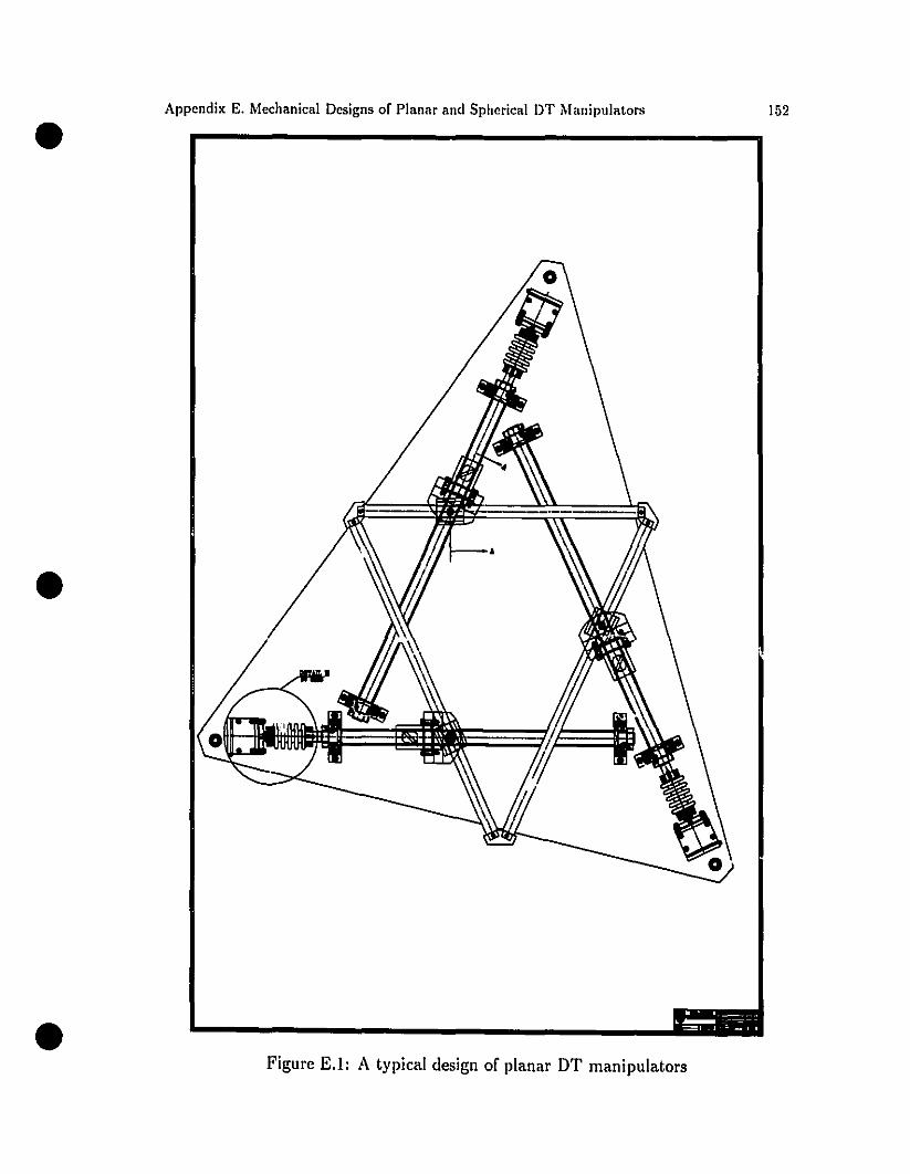
Appcndix E. Mcchanical Designs of PIanar and Spherical DT Manipulators

Figure E.l: A typical design of planar DT manipulators

152

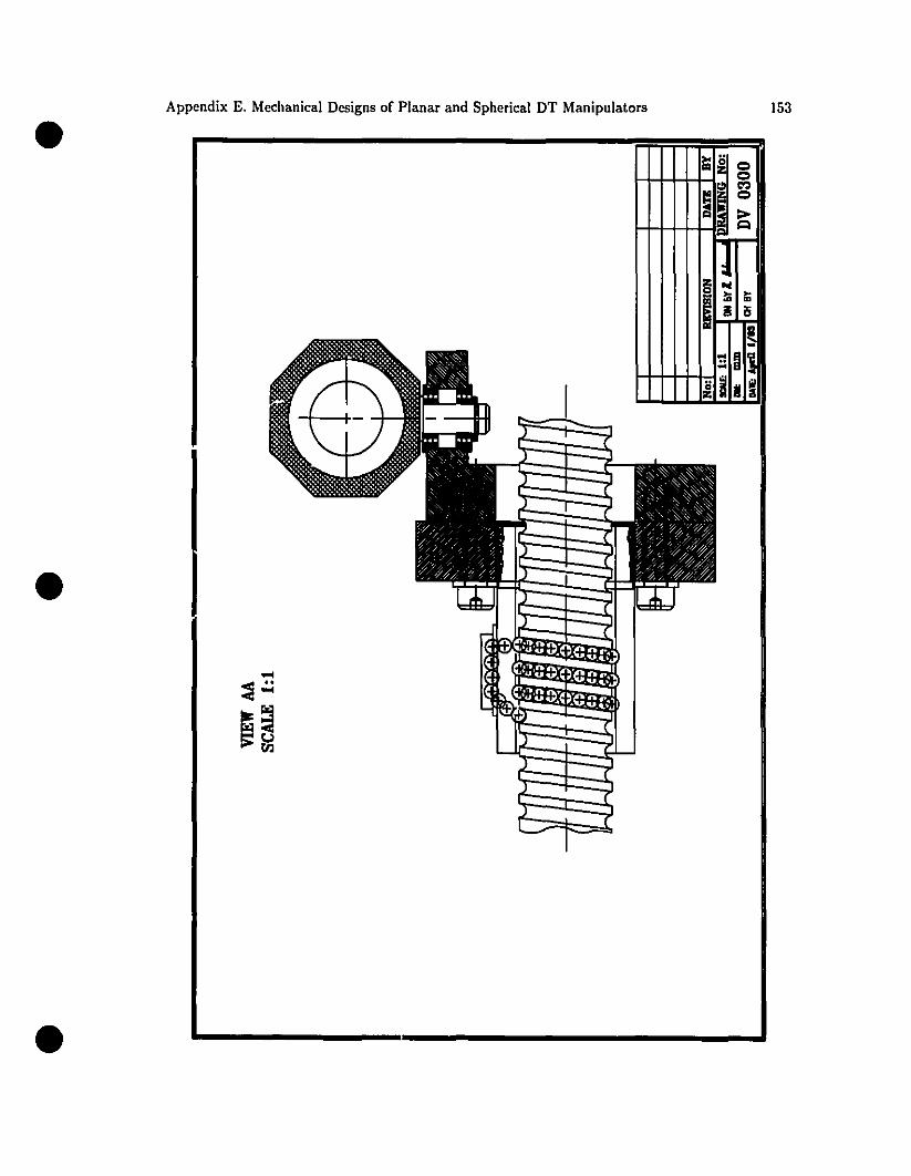
•Appendix E. Mechanical Designs of Planar and Spherical DT Manipulators 153

•

•

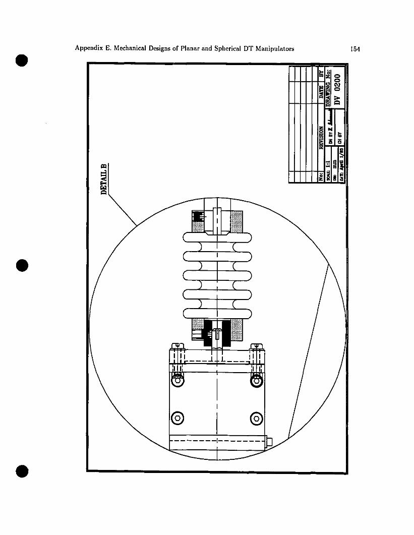
• Appcndix E. Mcchanical Designs of Planar and Sphcrical DT Manipulators 154

~~ 00

" N

U 0

"il! ~"

JI: .."1~ ~

li i5Il

~9

d ~ ~

- - - - - - -1- - - - - --

@

Il!IIIIIII

@

•

•

•

•

•

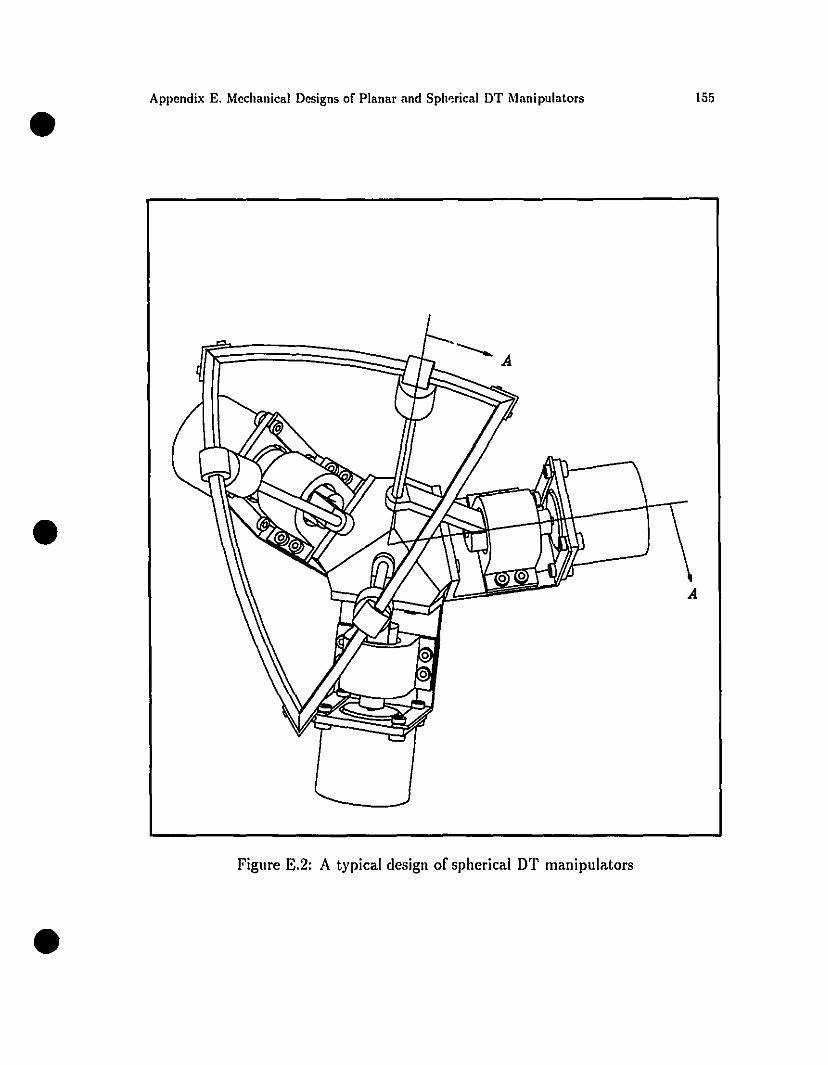
Appendix E. Mechanical Designs of Planar and Spherical DT Manipulators

---- A

Figure E.2: A typical design of spherical DT manipulators

155

A

•

•

•

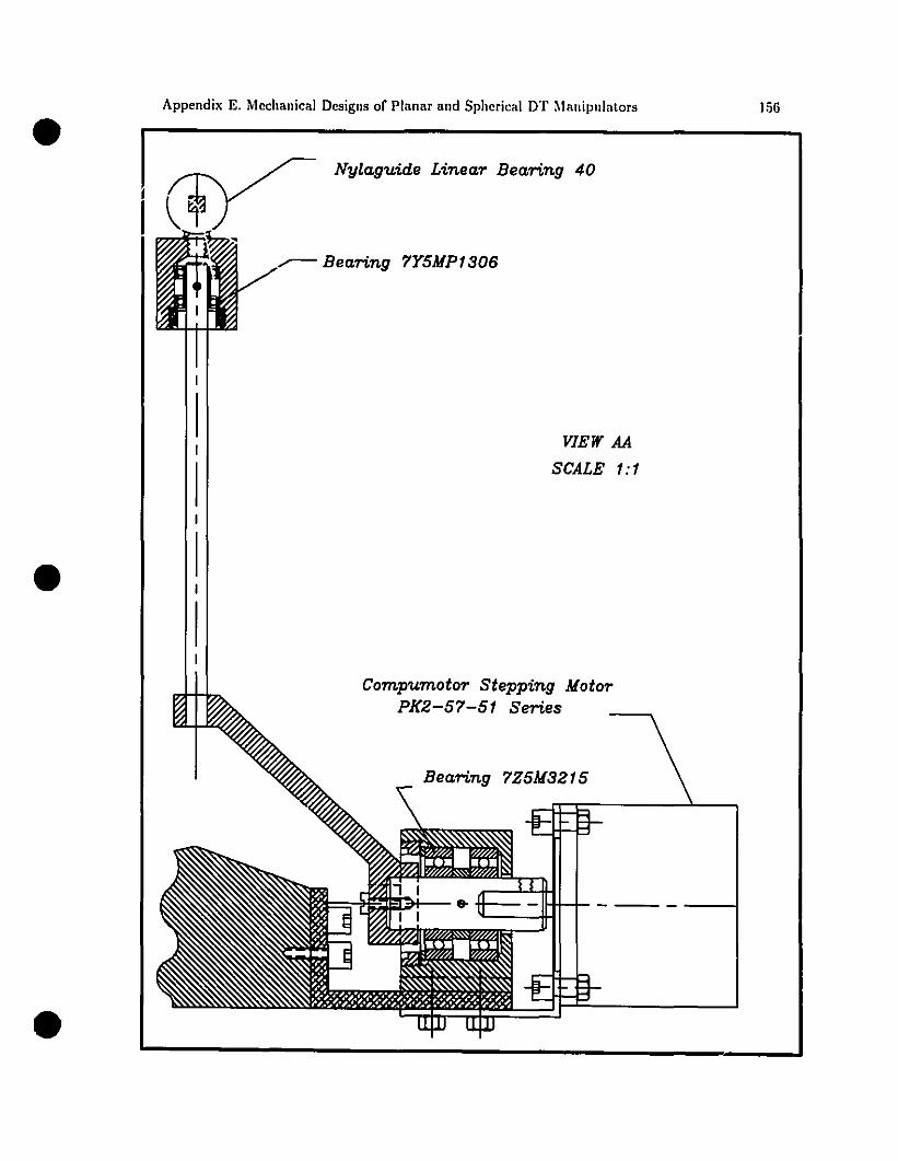
Appendix E. Meehanieai Designs of Planar and Spherieal DT Manipnialors

Nylaguide Linear Bearing 40

,.- Bearing 7Y5MP1306

VIEW AA

SCALE 1:1

Compumotor Stepping MotorPK2-57-51 Series

Bearing 7Z5M3215

156