Embed Size (px)
Citation preview
N Ui11 tILE WVQ '¢N
(7)Technical Report 1022
I--Analysis and Control
of Robot Manipulators
with Kinematic
Redundancy
Pyung H. Chang
MIT Artificial Intelligence Laboratory
S F11 FA r 9,98
rads d.jiii.bw Pubbe "dem"'Fad
UNC LASS IF IEDSECURTv CL AS55IC &!ION or TNIS PAGE (Wi,.,. Data [email protected])_
READ INSTRUCTIONSREPORT DOCUMtHTATION PAGE BEFORE COMPLETING FORMI. REPORT NUMBER 12. GOVT ACCESSION4 NO. A. RECIPIENT'S CATALOG NUMBER
AI-TR 1022
4. TITLE fond Subillie S. TYPE Of REPORT A PERIOD COVERED
Analysis and Control of Robot Manipulators technical report* with Kinematic Redundancy a. EORMING ORG.REPORT NUMBeR
7. AUTHOR@) I. CONTRACT OR GRANT NUMBERfet)
Pyung Hun Chang N0001I4-80-C-0505
NOQ 1 4-86-K-06859. PERFORMING ORGANIZATION NAME ANO ADDRESS I0. PROGRAM FLEUENT. 1111JECV. TASK
Artificial Intelligence Laboratory AE OKUI UBR
545 Technology SquareCambridge, MA 02139 ______________
I$. CONTROLLING OFFICE NAME AND ADDRESS 12. REPORT DATE
Advanced Research P rojects Agency Februar 19881400 Wilson Blvd. IS. NUMBER OFr PAGES
Arlington, VA 22209 1 3214. MONITORING AGENCY NAME It AODRESS(II different from Controlling Office) 1S. SECURITY CLASS. (of this report)
Office of Naval Research UNCLASSIFIEDInformation Systems _________________
*Arlington, VA 22217 ISa. 01CL SSI IC ATO/ QWNGRADING
16. DISTRIBUTION STATEMENT (of Oio Reort)
Distribution is unlimited
17. DISTRIBUTION STATEMENT (01 WOf abstract entered In 81109 20, it 41i11101611 frm Report)
IS. SUPPLEMENTARY NOTES
None
19I. KEY WORDS (Continue on reverse sieH ii e 01eceee nmd 114110111111 6F' block u ber)
kinematic controlredundant manipulators
20. ABSTRACT (Continue an favor** aide It 1eeeeeelY And 11101111FS? block a eR)1160
A closed-form solution formula for the kinematic control of manipulators withredundancy is derived, using the Lagrangian multiplier method. Differentialrelationship equivalent to the Resolved Motion Method has been also derived.The proposed method is proved to provide with the exact equilibrium state forthe Resolved Motion Method. This exactness in the proposed method fixes therepeatability problem in the Resolved Motion Method, and establishes a fixed
DD I "'Rm, 1473 EDITION orF Nov5 asis OBSOLETE UCLS FIES/N 0!02-014- 6601 I
SECURITY CLASSI'ICAION 4QF thiS PAGE (When Does Bnftrw
aA
Block 20 cont.
transformation from workspace to the joint space. Also the method, owing to the
exactness, is demonstrated to give more accurate trajectories than the Resolved
Motion Method.In addition, a new performance measure for redundancy control has been de-
veloped. This measure, if used with kinematic control methods, helps achieve
dexterous movements including singularity avoidance. Compared to other mea-
sures such as the manipulability measure and the condition number, this measuretends to give superior performances in terms of preserving the repeatability prop-erty and providing with smoother joint velocity trajectories.
Using the fixed transformation property, Taylor's Bounded Deviation Paths
Algorithm has been extended to the redundant manipulators.
AcoessIon For
PTTS GWAIDTI TABUnannomeed 0Justltioation
Distribution/
Availability Codes
fAvai -and/orDist Special
N "
C.
6!
--4
0l
I1ANALYSIS AND CONTROL OF ROBOT MANIPULATORS
WITH KINEMATIC REDUNDANCY
BY
PYUNG HUN CHANG
B.S.(1974) Mechanical EngineeringSeoul National University, Seoul, Korea
M.S.(1977) Mechanical EngineeringSeoul National University, Seoul, Korea
Submitted to the Department of Mechanical Engineering
in partial fulfillment ofthe requirements for the Degree of
Doctor of Philosophy in Mechanical Engineering
at the
Massachusetts Institute of Technology
May 1987
@ Massachusetts Institute of Technology
Signature of AuthorDepartment of Mechanical Engineering
May 12, 1987
Certified byBerthold K. P. Horn
Department of Electrical Engineering and Computer ScienceThesis Supervisor
Accepted byAin A. Sonin, Chairman
Departmental Graduate CommitteeDepartment of Mechanical Engineering
_ii+ 11 I~ k iiI1
Analysis And Control Of Robot Manipulators
With Kinematic Redundancy
by
PYUNG HUN CHANG
Submitted to the Department of Mechanical Engineeringon May 1, 1987 in partial fulfillment of
the requirements for the Degree ofDoctor of Philosophy in Mechanical Engineering
ABSTRACT,A closed-form solution formula for the kinematic control of manipulators with
redundancy is derived, using the Lagrangian multiplier method. Differential*relationship equivalent to the Resolved Motion Method has been also derived.
The proposed method is proved to provide with the exact equilibrium state forthe Resolved Motion Method. This exactness in the proposed method fixes therepeatability problem in the Resolved Motion Method, and establishes a fixedtransformation from workspace to the joint space. Also the method, owing to theexactness, is demonstrated to give more accurate trajectories than the ResolvedMotion Method.
In addition, a new performance measure for redundancy control has been de-veloped. This measure, if used with kinematic control methods, helps achievedexterous movements including singularity avoidance. Compared to other mea-sures such as the manipulability measure and the condition number, this measuretends to give superior performances in terms of preserving the repeatability prop-erty and providing with smoother joint velocity trajectories.
Using the fixed transformation property, Taylor's Bounded Deviation Paths
Algorithm has been extended to the redundant manipulators. ( g I. ) -
Thesis Supervisor: Dr. Berthold Klaus Paul Horn
Professor of Electrical Engineering and Computer Science
Acknowledgment: This report describes research done at the Artificial In-telligence Laboratory of the Massachusetts Institute of Technology. Support for thelaboratory's artificial intelligence research is provided in part by the Office of NavalRebearch UnIversity Research Initiative Program under Office of Naval Researchcontract N00014-86-K-0685, in part by the Advanced Research Projects Agcncy ofthe Department of Defense under Office of Naval Research contract N00014-80-C-0505, and in part by the Systems Development Foundation.

Acknowledgements
Many people contributed to this thesis. I will attempt to recall the major
contributions here.
My adv isor Berthold K. P. Horn was the guiding force behind the thesis, whom
I deeply thank. He first suggested to me to work on the redundant manipulators,
provided advices on the direction of the thesis, and then helped with insights,
encouraged, and generously supported me throughout my thesis work at the MIT
Artificial Intelligence Laboratory. He also read through several drafts carefully,
returning valuable comments.
I also thank the other members of my committee: Jean J. Slotine and Ken
Salisbury. Jean has been helping me in various ways for several years. He espe-
cially gave me some important insights about sliding mode control techniques. I
also appreciate his effort and understanding as the chairman of the committee,
which were of great help to me. I would like to thank Ken sincerely for his help
in many ways. Out of a genuine interest in my research, he gave me many helpful
suggestions in solving some of the problems that I had faced. Above all, his will-
ingness to be available without reservation, together with friendliness, has been
especially consoling and encouraging during the period when my advisor was on
sabbatical leave.
I also thank Toms Lozano-Pdrez for his excellent teaching through the course
in robot manipulation. Besides, his comments and suggestions in the first half of
my thesis were valuable. In addition, I recall with thanks the kindness and favor
TomAs showed to me on some occasions.
T would like to thank the MIT Al Lab, directed by Patrick Winston, for
providing the excellent environment, abundant resources, and generous financial
support, which made this thesis work much easier. Additional thanks go to Chae
2
' '
1 1
t; ;11 1 ;
0
An for providing me various helps including prayers; Neil Singer for helping me
in computation problems including advices on plottings.
Members of the Gate Bible Study at MIT have supported me by their loving
care and prayer. My parents and parents-in-law have supported me and encour-
aged me throughout the seven years at MIT. Now, I cannot recall my two great
sons, Chai and Jun, without appreciating and being proud of what they have
been and done to me: so disciplined and mature for their ages.
Finally I can never thank enough my wife, Minja, who has demonstrated her
love by supporting me both spiritually and emotionally, with such remarkable
patience and sensitivity.
3
Contents
1 Introduction 71.1 Background Study .. .. .. .... .... ... .... .... .... 8
1.1.1 Inverse Kinematics For Trajectory Control. .. .. .. ..... 81.1.2 Kinematically Redundant Manipulators .. .. .. .... .. 111.1.3 Performance Measure For Singularity Avoidance. .. .. ... 14
1.2 Objectives .. .. .. ... .... ... .... ... .... .... .. 181.3 Overview of the Thesis .. .. .. ... ... .... .... ... ... 19
2 The Proposed Method for the Kinematic Control 212.1 Introduction .. .. .. .. .... .... ... .... .... ... .. 212.2 Derivation of the Proposed Equation .. ... ... .... ..... 222.3 Characteristics .. .. .. .... .... ... .... .... ... .. 262.4 Computational Consideration .. .. .. ... .... .... ... .. 28
2.4.1 Motion strategy .. .. ... .... .... ... .... ... 292.4.2 Computational Effort at Each Iteration Step .. .. ... .. 302.4.3 Number of Iterations. .. .. .. .... ... .... ...... 312.4.4 Minimum Number of Via Points .. .. ... .... ... .. 32
2.5 Comparison with Other Methods. .. .. ... ... .... ...... 332.5.1 Relationship with Luh's Expression .. .. .. ... ... ... 342.5.2 Relationship with Extended Jacobian Method. .. .. .. .. 34
2.6 Conclusion .. .. ... .... ... .... .... ... .... ... 35
3 Relationship with Resolved Motion Method 373.1 Introduction .. .. .. .. .... .... ... .... .... ... .. 37'3.2 Resolved Motion Method .. .. ... .... .... ... .... .. 38
3.2.1 The Method and Its characteristics .. .. .. ... .... .. 38:3.2.2 Repeatability' Problemii.. .. .. ... .... .... ...... 10
3P.3 Relationship between the Two Methods.. .. .. .. ... .... .. 413.3.1 Equilibrium Slate .. .. ... .... .... ... .... .. 423.3.2 Differential Relationship. .. .. .. .... .... ... ... 430.3.3 Summary. .. .. .. .. .... ... .... .... ... ... 44
3.4 Computational Consideration .. .. .. .... ... .... ...... 453.4.1 Obtaining equilibrium States. .. .. ... .... .... .. 453.4.2 Obtaining Joint Velocitv .. .. .. ... .... ... ..... 47
3..5 Conclusion .. .. ... .... ... .... .... ... .... ... 48
4 Numerical Experiment on Kinematic Control Methods 504.1 Introduction .. .. .. .. .... .... ... .... .... ..... 504.2 System Descriplon. .. .. .. .... ... .... .... ... ... 514.3 Procedures. .. .. .... ... .... .... ... .... ...... 534.4 Results................. .. . . .... . ... . ..... .. .. .. .. 554.5 Discussions. .. .. ... .... .... ... .... .... ... .. 63
5 Development of A Dexterity Measure 685.1 Introduction .. .. .. .. .. ... ... ... ... ... ... ..... 685.2 Review of Singularity and Redundancy. .. .. .. .... ... ... 70
5.2.1 Singularity .. .. ... ... .... .... .... ... ... 705.2.2 Kinematic Redundancy. .. .. .... ... .... ...... 72
5.3 A New Concept of Distance from Singularity in Redundant Case .735.4 The Derivation of A New Performance Measure .. .. .. ... ... 775.5 The Property of The Measure .. .. .. ... .... ... .... .. 785.6 Conclusion .. .. ... .... .... ... .... .... ... ... 79
6 Relationship and Comparison with other Measures 826.1 Introduction .. .. .. .. .. ... ... ... ... ... ... ..... 826.2 Relationship with Other measures. .. .. .... .... ... ... 83
6.2.1 the relationship to the manipulability measure .. .. .. .. 836.2.2 Relationship with the condition number .. .. .. .... .. 85
6.3 Comparison of Performance measures .. .. ... .... .... .. 876.3.1 Overcoming singularity .. .. ... .... .... ... ... 886.3.2 Preserving the aspect and its effect to the repeatability
problem .. .. .. ... .... .... ... .... .... .. 956.3.3 Discontinuity effects .. .. ... ... .... .... ... .. 99
6.4 Conclusion. .. .. .... .... ... .... .... ... ..... 100
7 Conclusion 112
*Appendices 115Appendix 1: Taylor~s Algorithm. .. .. ... ... ... ... ... ... 115Appendix 2: The Derivation of The Extended Jacobian Method. .. ... 116Appendix 3: Equilibrium State Relationship. .. .. .. .. ... ... ... 17Appendix 4: Proof of Theorem .. .. .. ... .. .... ... ... ... 119
S5
I0r 111 11 1 I
Chapter 1
Introduction
The kinematic control of kinematically redundant manipulators has become an
important subject of study, owing to the growing interests in redundant robot
manipulators. Unfortunately, most of the existing control algorithms are in a
differential form based on the pseudoinverse matrix, subject to usual problems
resulting from linearization. The algorithms that instead use a direct mapping,
are not compact and closed-form, and not applicable to all manipulators. Fur-
thermore, little is known about the relationship between direct mapping methods
and the differential approach for redundant manipulators. One motivation of this
thesis is the desire to develop such a compact yet general formula that enables
direct mapping, and to understand the relationship between this formula and
* algorithms in differential form.
Another motivation comes from the observation that the degree of redundancy
cannot sufficiently describe how far a manipulator is from singularity. In other
words, with the same degree of redundancy, there are relatively different degrees
of distance from singularity. Surprisingly, little research, to our knowledge, has
dealt with this fact. Hence, to develop a satisfactory concept of relative degrees
of redundancy is another major purpose. Then, from this concept, we derive
7
a practical performance measure that can be used for singularity avoidance or
dexterity achievement in the redundant manipulators.
The introduction is organized as follows. In Section 1.1, we present the back-
ground of the motivations mentioned above. In Section 1.2, then, we define the
problems and objectives of this thesis. Finally, in Section 1.3, we present the
overview of the organization of this thesis.
1.1 Background Study
1.1.1 Inverse Kinematics For Trajectory Control
Manipulator Kinematics
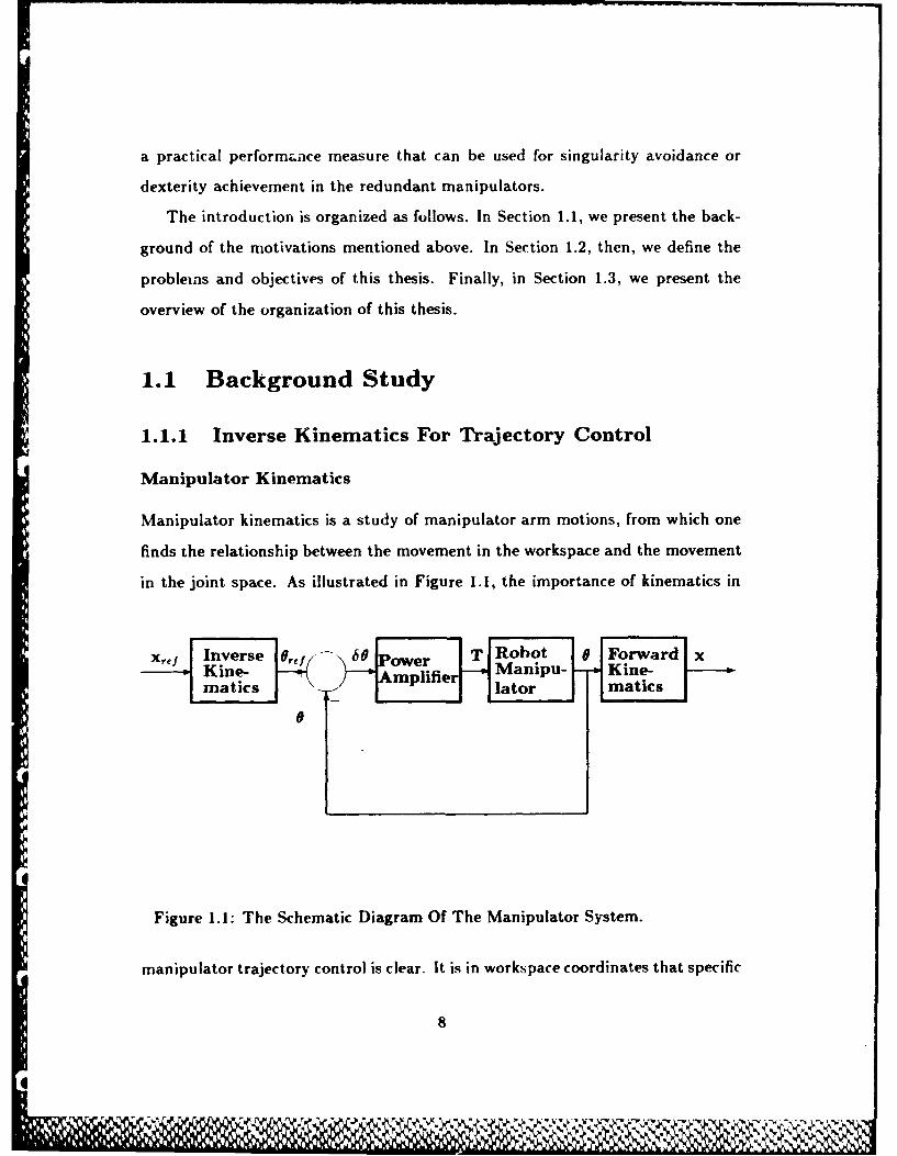
Manipulator kinematics is a study of manipulator arm motions, from which one
finds the relationship between the movement in the workspace and the movement
in the joint space. As illustrated in Figure 1.1, the importance of kinematics in
Xref Inverse -ref 6 8ower T Robot 0 Forward xKine- mplifier Manipu- Kine-matics lator matics
9
Figure 1.1: The Schematic Diagram Of The Manipulator System.
manipulator trajectory control is clear. It is in workspace coordinates that specific
d8
_N
12,11
tasks we desire are usually expressed; whereas it is in the joint coordinates that
the actuator movements are described. Therefore, kinematics is a fundamental
tool directly connected to the performance in manipulator trajectory control.
Forward Kinematics and Inverse Kinematics
Manipulator kinematics, hence, includes two important problems. One is to find
the location' of the manipulator in workspace coordinates from its joint coor-
dinates and the other is to find the joint coordinates from the location in the
workspace coordinates. The former is called the forward kinematic problem; the
latter, being the inverse problem, is called the inverse kinematic problem.
Of the two problems, the forward kinematic problem is the simpler one since
a set of joint coordinates unambiguously determines a unique location in the
workspace. Furthermore, the solution can usually be expressed in a symbolic
form, which can be easily evaluated given a set of joint coordinates (Paul,1981).
The inverse kinematic problem, on the other hand, is more complicated because,
given a location in the workspace, there are multiple sets of corresponding joint
coordinates. More importantly, there do not exist, in general, closed-form solu-
tions, except for some kinematic structures of manipulators. Pieper(1968), by
the way, presented the criteria that guarantee the existence of a closed-form solu-
tion. Thus, if a manipulator structure does not belong to this category, one has
to find solutions by numerical methods, typically iterative ones.
Resolved Motion Method and Inverse Kinematic Method for Non-
Redundant Manipulators
To numerically solve the inverse kinematic problem, there are two approaches: one
that uses the linear relationship between the differential joint displacement and
'location consists of position and orientation.
9
differential end effector displacement; and one that uses the direct mapping from
workspace to joint space. The former, originally proposed by Whitney(1969,1972)
and subsequently used by(Paul,1981; Featherstone,1983), is called the Resolved
Motion Method; while the latter, investigated by (Albala,1979; Konstantinov et
al,1982; Gupta et al,1985; Goldenberg et al,1985; Angeles,1985; Wampler,1986),
is simply called the Inverse Kinermatic Method.
More specifically, the Resolved Motion Method first differentiates the desired
trajectory of the end effector to obtain velocity. Then, this Cartesian velocity is
mapped into the joint velocity, using the inverse of the Jacobian matrix. Finally,
the joint velocity is integrated to determine the joint displacement.
The iterative Inverse Kinematic Method, on the other hand, directly solves
the nonlinear kinematic equations, without linearizing them, for a given location
in workspace. Note, however, that the updating process at each iteration step of
a numerical method for solving the nonlinear kinematic equations can be viewed
as an incremenal process like the Resolved Motion Method. With this view,
then, the essential difference between the two approaches may be considered the
number of iterations: The Resolved Motion Method can be considered a one
"-iteration Inverse Kinematic Method without any built-in convergence criteria.
Comparison of the two methods
The Resolved Motion Method, thus, has some weak points:
" The method has intrinsic inaccuracy because of the linear approximation
characteristics of the Jacobian matrix; thus it accumulates errors, which
become larger as the velocity increases.
" The method, being a rate equation, is not self-starting: given a location of
the end effector, corresponding joint values cannot be determined without
using other methods.
010
The Inverse Kinematic Method without closed-form solution, on the other
hand, usually requires more computational effort than the other method. So
this method is not efficient when high accuracy is not needed. Even when high
accuracy is required, in order to be practical for the real-time control purpose,
the method may need some additional numerical schemes such as interpolations
between knot points (Paul,1975; Paul,1979; Taylor,1979). Moreover, for some
applications that require to resolve joint velocity and acceleration as well, it has
an intrinsic disadvantage. Yet, the Inverse Kinematic Method is still attractive
because of the direct mapping from the workspace to joint space, fixing the afore-
mentioned problems of the other method.
1.1.2 Kinematically Redundant Manipulators
Kinematic Redundancy
A kinematically redundant robot manipulator is a manipulator that has more
degrees of freedom than necessary to place the end effector at a desired location.
For example, if we want to place the end effector in a three dimensional-space,
we need six degrees of freedom: three for translation and three for orientation.
Thus, a robot manipulator with more than six degrees of freedom is kinematically
redundant in the three-dimensional space.
Use of Redundancy
The major advantages of adding redundant degrees of freedom to a robot manip-
ulator are as follows:
1. One achieves greater dexterity in maneuvering in a workspace with obsta-
cles.
2. One can avoid singular configurations of the manipulators.
*111 M . .. . .
0 1 1 11 11
Because of these significant advantages, an increasing amount of research has fo-
cused on the kinematically redundant manipulator, and the progress in this field
has been rapid. More specifically, to avoid obstacles, several researcher such as
(Yoshikawa,1984; Maciejewski,1985; Espiau,1985; Nakamura,1985; Baillieul,1986)
have used the kinematical redundancy. Meanwhile the effort to avoid singular-
ity through the use of redundant manipulators is found in the works by (Whit-
ney,1972; Yoshikawa,1984; Hollerbach,1985,Baillieul,1985; Luh et al,1985; Naka-
mura,1985a). Besides, the use of the kinematic redundancy has been proposed for
constraining the joint variables within their physical limits (Liegeois,1977), or for
minimizing joint torques (Hollerbach,1985), or for minimizing the kinetic energy
due to joint velocity (Whitney,1972).
Redundancy control
Mathematically, the inverse kinematic problems of redundant manipulators are
under-determined problems: more variables(joint variables) than constraints(kinematic
equations). In order to solve equations we need to impose extra constraints.
These additional constraints sometimes tend to be imposed out of necessity to
fully specify the under-determined condition; or sometimes are used, on purpose,
to achieve additional performances objectives as mentioned above. The former
tendency was shown in (Whitney,1972), where the joint velocity was obtained by
using the pseudoinverse of the Jacobian matrix to resolve the under-determined
joint velocities.
The latter case, active use of redundancy called the redundancy control, was
first proposed by Liegeois (Liegeois,1977). He used, in addition to the same pseu-
doinverse term as above, the null space term, where he included the gradient
vector of a scalar function that represents the desired performance. This gradi-
ent vector by the way, if used with the null space of the Jacobian matrix, forces
12
WII
the joints to move toward the direction where the scalar function has the op-
timal value at that instant. This formulation of solution, owing to the ease of
including the desired performance, has been rather extensively used to achieve
various performances as mentioned above (Klein and Huang,1983; Maciejewski
and Klein,1985; Nakamura,1985a; Hollerbach and Suh,1986).
Resolved Motion Method and Inveirse Kinematic Method
In much of the research just mentioned - regardless of whether the null space is
actively used or not, or regardless of which performance is desired - the motion
is resolved in the differential form. More specifically, the differential displacement
(or velocity) of the end effector is mapped into the differential joint displace-
ment (or velocity) now by using the pseudoinverse of the Jacobian matrix, and
then incrementally determines the joint displacement. This technique, thus, is
essentially the same as the Resolved Motion Method in the nonredundant case;
the only difference is that the pseudoinverse is used instead of the inverse of the
Jacobian matrix. 2
In contrast to this direction of research, relatively little research for kine-
matically redundant manipulators, e.g., (Benati et al,1982; Hollerbach,1985; Oh
et ai,1984; Benhabib et al,1984,1985) has involved the direct mapping - the
counterpart of the Inverse Kinematic Method in the nonredundant case. In the
redundant case too, there exist in general no closed-form solutions; only if cer-
tain conditions are met by the manipulator structure, then a part of solution is
given. For example, in (Benati et al,1982, Hoilerbach, 1985) only some of the
joint variables were obtained symbolically. To obtain these solutions the manip-
ulator structure and the number of degrees of freedom were fixed, explicitly in
(Hollerbach,1985) and implicitly in (Benati,1982).
-Hence we will call tins resolhition technique the Resolved Motion Method, too.
13
1 I
I
Comparison of the two methods in the redundant case
Of the two methods, the Resolved Motion Method and the Inverse Kinematic
Method, the advantages(and disadvantages) of the one method over the other in
the nonredundant case were compared in the previous subsection. The comparison
still holds in the redundant case, since each of the methods is essentially the same
as its counterpart in the nonredundant case.
In addition, another significant drawback in the Resolved Motion Method was
pointed out in (Klein,1983): the lack of repeatability, the ability to repeat the
same joint values for repeated end effector motion. This problem, however, does
not occur when direct mapping is used.
6 Meanwhile, an additional difficult task for Inverse Kinematic Method, on the
other hand, is to rationally (or optimally) use the extra degrees of freedom when
achieving the additional objectives. Often, this optimization procedure being
rather complicated, the overall inverse kinematic process results in a series of
iterative procedures. This time, the shortcoming is not so serious in the Resolved
Motion Method, because of the simple null space expression.
Therefore, the comparison clearly shows that one method is complementary
to the other, indicating one desired direction in which a kinematic control formula
should be developed: a formula that provides with the direct mapping, and that
is as concise and general as the Resolved Motion Method.
1.1.3 Performance Measure For Singularity Avoidance
Using a quantitative measure that represents the desired performance is a ben-
eficial method for the analysis, design, and control of engineering systems, as
follows:
14
=ol
" one can evaluate the performance of a given system and analyze the system,
by estimating this measure; or
" one can design a system that achieves the performance in a certain degree,
by maximizing(or minimizing) this measure; or
" one can control, on the on-line basis, a given system to achieve it, by max-
imizing the measure at each moment,
without having to rely solely on experience and intuition.
In the robotic system, also, various performance measures have been incorpo-
rated to quantify desired performance features listed in the previous subsection.
Dexterity measure
One of these performances was the ability to avoid singularity, or in a broader
sense the ability to dexterously move the end effector to an arbitrary location
within the workspace, without getting into singular configurations. To quan-
titatively represent the ability, which may be called dexterity, several perfor-
mance measures have been proposed (Yoshikawa, 1985a, 1985b; Uchiyama,1985;
Maciejewski,1985; Salisbury; 1982). These measures are the determinant, the
condition number, and a few combinations of singular values, of the Jacobian
matrix J - through which, by the way, the end effector movement is achieved.
Determinant
In linear algebra, the determinant of a matrix has been an important measure
used to test the invertibility of the matrix and its nearness to singularity. Ac-
cordingly the determinant of the Jacobian matrix has been tried for the dexterity
measure for both nonredundant and redundant manipulators. For nonredundant
manipulators, for instance, the determinant has been used as a measure of de-
generacy for the analysis of the wrist configurations(Paul and Stevenson, 1983).
15
For redundant manipulators, on the other hand, Yoshikawa(1984) has proposed
a measure called manipulability defined as the square root of the determinant ofjjT .This measure is viewed as a generalized concept of the determinant, because
of the followings:
" the manipulability reduces to the regular determinant in the nonredundant
case.
" the manipulability become zero, when workspace rank reduces at singularity,
just as the regular determinant of a square Jacobian matrix does.
" since the singular values of jjT have the square values of those of J, the
determinant of jjT may be regarded as if it were the square of the regular
determinant of a square Jacobian matrix.
Condition number
Meanwhile, since the condition number of the Jacobian matrix is another im-
portant measure that also indicates the nearness of a matrix to singularity, it
has been proposed for a dexterity measure(Salisbury,1982). It is noteworthy that
this measure was initially used to determine the configuration that minimizes the
propagation from the torque error to the force error - equivalently, the velocity
error propagation from joint space to workspace - for nonredundant manipula-
tor.
Singular values
The determinant and the condition number can be also expressed in terms of sin-
gular values of the Jacobian matrix: the former is the product of all the singular
0values, the latter the ratio of the largest to the smallest singular value. Since
the minimum singular value becomes zero when the matrix is singular, and ap-
proximately determines the worst limits of the two measures, the value itself was
suggested as a new measure(Klein,1985). In addition to its simple expression,
16
,0 - ;.. .
the measure has a relatively clear physical meaning: it may be interpreted as
the minimum responsiveness in end effector velocity due to a unit change in joint
velocity(Klein,1985).
Besides, the geometric mean and harmonic mean of singular values have been
proposed for the dexterity measures(Yoshikawa,1985b), which may be viewed es-
sentially as variations of aforementioned measures.
Common features
The features common to all these measures are as the following:
" They indicate the presence of singularity: when singular, the value of these
measures become zero, except for the condition number, the value of which
becomes infinity.
" Their absolute values - inverse of the value in the case of the condition
number - appear to represent, in one way or another, the farness or dis-
tance from singularity. That is, the larger the value, the farther is the
manipulator from a singularity.
In the case of redundant manipulators, however, these measures do not ex-
plicitly indicate the successive changes in the available degrees of freedom as long
as the workspace rank is preserved. For instance, suppose we have a five d.o.f.
manipulator which is to move in a three-dimensional workspace, hence having
two degrees of redundancy. Although the manipulator happens to lose one degree
of freedom, or even two, the measures do not necessarily indicate that fact.
Problems when losing d.o.f.
Losing degrees of freedom may not in itself be a serious drawback, as long as
the workspace rank is fully preserved so that the desired location of the end
effector can be achieved by joint variables. Yet, what may be of more concerns
17
are potential problems that are expected to arise - from the similar experience
in the nonredundant case - when degrees of freedom are lost. More specifically
speaking, in the nonredundant case, the point where the degrees of freedom are
lost - namely the singular point - is in fact the boundary of switching from one
set of joint solution to another (Uchiyama,1979). Once that switching happens,
the manipulator tends to stay in the new kind of joint configuration different
from the previous kind, thus causing another pattern of repeatability problem.
Besides, when the switching arises, usually there are accompanying discontinuity
in motion, resulting in large joint velocities. The same problems are expected
in the redundant case, since in this case too there exist multiple solutions of
different kinds (Borrel,1986) whose boundaries are the points where the degree of
-eedom decreases. It appears, however, that these nontrivial problems tend to be
veiled because of the fact that owing to the redundancy the switching can happen
without causing the more serious problem, singularity. To our knowledge, there
have not appeared any analysis on these problems for redundant manipulators,
and any performance measures that are intended to prevent them.
1.2 Objectives
The objective of this thesis, broadly speaking, is to study trajectory control of
kinematically redundant manipulators, focusing on the kinematic problems men-
tioned in the first subsection.
To this end there are two major goals. The first goal is to develop a general
closed-form method for the inverse kinematics of manipulators with kinematic
redundancy. This method is similar to the formulation of the Resolved Motion
method, in actively using kinematic redundancy; but it is different in choosing
direct mapping from the workspace to joint space. Under the first goal, however,
*18
0AI
L M R1121r
I
to understand the relationship between the inverse kinematic method and resolved
motion method is another intended purpose.
The second goal is to analyze the aforementioaed relative distance of redun-
dant manipulators, and to derive from this analysis a performance measure that
represents the dexterity of manipulator including singularity overcoming. This
performance measure is intended to be used either with on-line kinematic control
methods including the one developed from the first goal, or for off-line design
purposes. Besides, the relationship between the resulting measure and already
existing measures is to be examined.
1.3 Overview of the Thesis
In Chapter 2, a closed-form formula for inverse kinematics of kinematically re-
dundant manipulators is to be derived using the Lagrangian multiplier method.
This formula consists of a set of equations which, if added to the kinematic equa-
tions, fully constrain the initially under-determined problem. The mathematical
meaning and applications of the formula are examined. Then the relationship
between the formula and already existing similar methods is investigated.
In Chapter 3, the qualitative relationship between the new method and the
Resolved Motion Method is examined. Then in the light of the relationship, the
repeatability problem is focused on.
In Chapter 4, the qualitative results obtained in Chapters 2 and 3 are verified
through numerical experiments. Finally numerical efficiencies of the two methods
are compared.
In Chapter 5, we propose a new concept representing the distance from sin-
gularity for kinematically redundant case. This concept is obtained by observing
the structure of the Jacobian matrix of redundant manipulators. Then, by using
01
I
the concept, we derive a new dexterity measure that can be used with either the
the formula obtained in Chapter 2 or the Resolved Motion Method.
In Chapter 6, the new performance measure is compared with two existing
performance measures: the manipulability measure and the condition number.
After their qualitative relationships are examined, the numerical experiments are
made with redundant manipulators to compare the effectiveness of each measure
in achieving dexterous movements. In the comparison, at the same time, the
repeatability problem, as well as the ability to preserve the kind of joint solutions
are to be observed.
Finally, in Chapter 7, concluding remarks are to be made.
20
I 2
Chapter 2
The Proposed Method for theKinematic Control
2.1 Introduction
In this chapter, we derive a general closed-form formula for the kinematic control
of redundant manipulators by using the Lagrangian multiplier method. This
formula, more specifically speaking, consists of an additional set of constraints
beside the kinematic equation.
The key features of this formula, beside its conciseness, are that it can contain
the performance measure as easily and generally as the Resolved Motion Method
with null space can (Liegeois,1977); and at the same time it is an inverse kine-
matic method. Among inverse kinematic methods for redundant manipulators,
we find similar approaches that use performance measures; but they lack some
of the features this formula has. Benati et a] (Benati,1982) suggested a method
using a general quadratic performance measure to be optimized, the resulting
control algorithm of which is quite complicated because of including the measure.
Benhabib et al (Benhabib,1984,1985) also used performance measures to achieve
21
HE10OMm
additional performances. These measures are optimized with a searching algo-
rithm under constraints on joint variables. The resulting algorithm becomes also
complicated.'
Rather, among the approaches using the Resolved motion method, we find
additional constraints in similarly concise forms, which could be also used in the
inverse kinematic method. Baillieul(Baillieul,1985), in the process of deriving a
rate equation called the extended Jacobian Method, obtained null space expres-
sions similar to the formula proposed here. Luh and Gu(Luh,1985) proposed
another expression of the null space in a generic form. We will investigate more
in detail about the relationship between the proposed formula and these methods.
After deriving the formula in Section 2.2, we will examine in Section 2.3 its
mathematical meaning and characteristics, as well as computational aspects in
Section 2.4. Then the relationship between the formula and the aforementioned
methods is covered in Section 2.5, and finally some concluding remarks are made
in Section 2.6.
2.2 Derivation of the Proposed Equation
In this section, we will derive extra equations which, together with the kinematic
equations of the manipulator, can fully specify the under-determined problem.
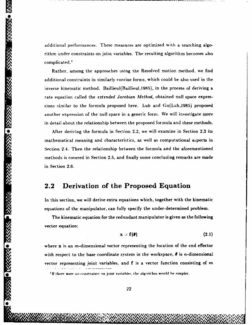
The kinematic equation for the redundant manipulator is given as the following
vector equation:
x f(9) (2.1)
* where x is an m-dimensional vector representing the location of the end effector
with respect to the base coordinate system in the workspace, 9 is n-dimensional
vector representing joint variables, and f is a vector function consisting of m
'if there were no con. traint.s on joint variahles, the .agnrithIil would be simpler.
22
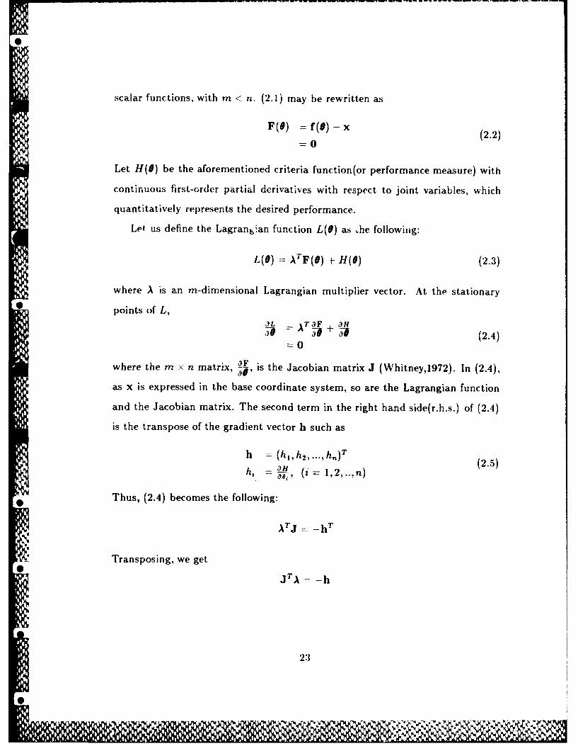
0scalar functions, with m < n. (2.1) may be rewritten as
F(0) f(0)- x (2.2)
=0
Let H(O) be the aforementioned criteria function(or performance measure) with
continuous first-order partial derivatives with respect to joint variables, which
quantitatively represents the desired performance.
Let us define the Lagran6ian function L(O) as ,he following:
L(0) = ATF(0) + H(0) (2.3)
where A is an m-dimensional Lagrangian multiplier vector. At the stationary
0 points of L,3L -T3F JH
3 0 T F0 4H (2.4)0
where the rn x n matrix, ' is the Jacobian matrix J (Whitney,1972). In (2.4),
as x is expressed in the base coordinate system, so are the Lagrangian function
and the Jacobian matrix. The second term in the right hand side(r.h.s.) of (2.4)
is the transpose of the gradient vector h such ash|
h = (h1, h2,...,) T (2.5)
h. = O_ , (Z'= 1, 2, n)
Thus, (2.4) becomes the following:
ATJ -_T
Transposing, we get
JTA -h
23
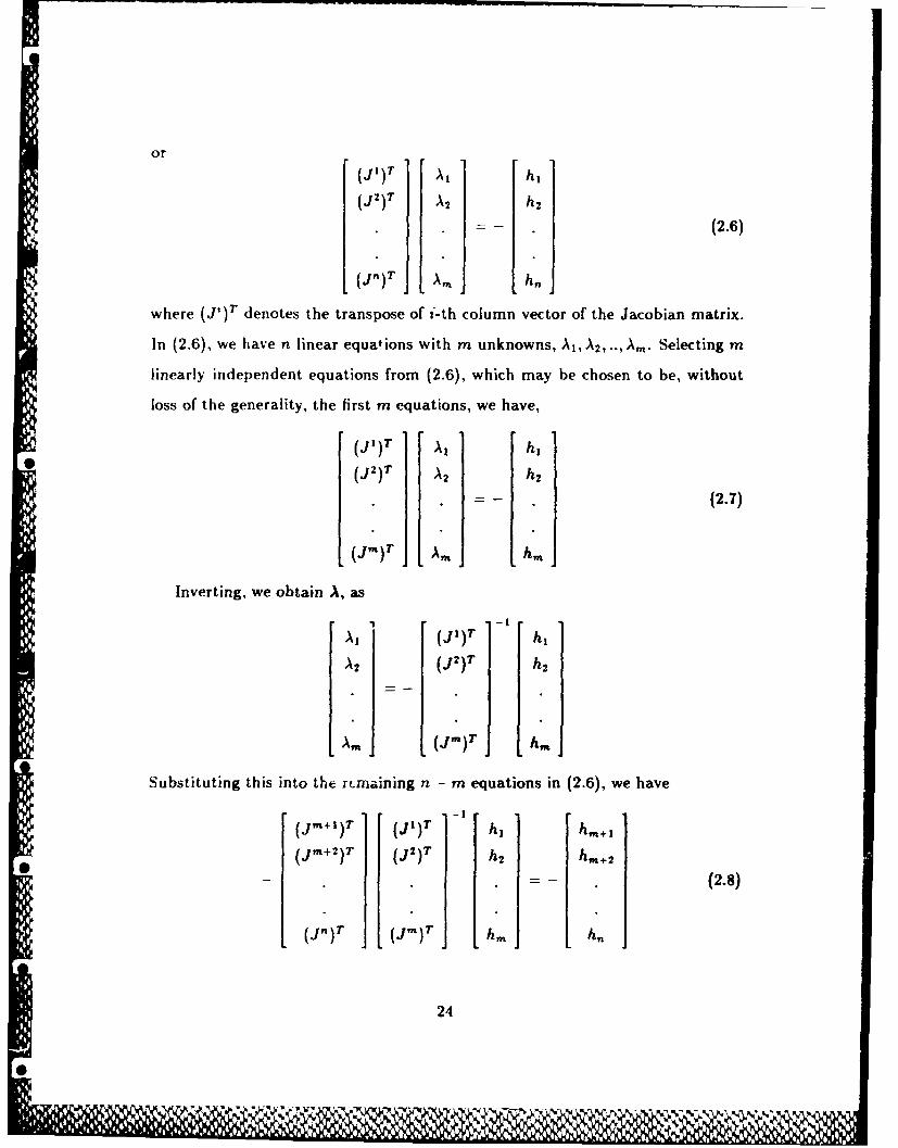
or(jI)T A, hi
(J2)T A2 h2
(2.6)
(jn)T An h,
where (Jt)T denotes the transpose of i*-th column vector of the Jacobian matrix.
In (2.6), we have n linear equations with m unknowns, Aj,A 2, .., A,. Selecting m
linearly independent equations from (2.6), which may be chosen to be, without
loss of the generality, the first m equations, we have,
(j1)T A, h
S(J2)T A2 h2
(2.7)
(Jm)T Anth
Inverting, we obtain A, as
A, (jl)T h
A2 (j2)T h
A,, (jm,)T hm
Substituting this into the rcrnaining n -m equations in (2.6), we have
(Jm+l)T (j1)T hi h.+i
(jmn+2)T (j2)T h2",
(2.8)
(jn)T (jm) T hm, ,
24
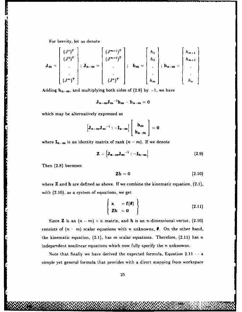
For brevity, let us denote
[ (jl)T (J,+1)T hi h.+ I
(j2)T (jm+2)T hm+2
,Jm ; Jn-m n h ;hn-m
(j-)? (jn)r L hm n
Adding hn-m, and multiplying both sides of (2.8) by -1, we have
Jn-mJm-'hn - hn-m = 0
which may be alternatively expressed as
[ininm-I :-I _MI hm 0Shn-m I
where ln-m is an identity matrix of rank (n - m). If we denote
Z [JnmJm- -In-rnl (2.9)
Then (2.8) becomes
Zh = 0 (2.10)
where Z and h are defined as above. If we combine the kinematic equation, (2.1),
with (2.10), as a system of equations, we get
, x =f(e) (.1
Zh =0
Since Z is an (n - m) x n matrix, and h is an n-dimensional vector, (2.10)
consists of (n - m) scalar equations with n unknowns, 0. On the other hand,
the kinematic equation, (2.1), has m scalar equations. Therefore, (2.11) has n
independent nonlinear equations which now fully specify the n unknowns.
Note that finally we have derived the expected formula, Equation 2.11 -- a
simple yet general formula that provides with a direct mapping from workspace
25
L
LM~ imm
to joint space. In (2.11), the additional set of constraints, (2.10), resolve the
redundancy -- at the inverse kinematic level - in such a way that, under the
kinematic constraint of (2.1), the criteria function, H(9), may be minimized.
Note also that (2.11) has to be solved numerically.
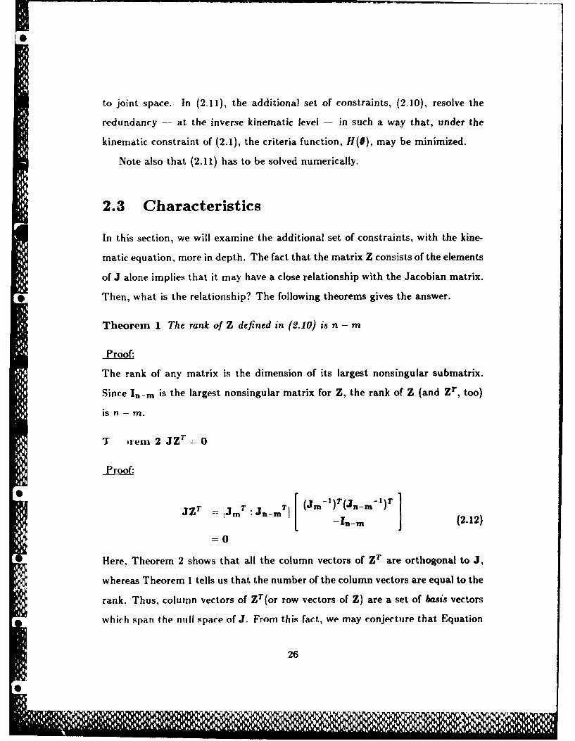
2.3 Characteristics
In this section, we will examine the additional set of constraints, with the kine-
matic equation, more in depth. The fact that the matrix Z consists of the elements
of J alone implies that it may have a close relationship with the Jacobian matrix.
*Then, what is the relationship? The following theorems gives the answer.
Theorem I The rank of Z defined in (2.10) is n - m
Proof:
The rank of any matrix is the dimension of its largest nonsingular submatrix.
Since In-r is the largest nonsingular matrix for Z, the rank of Z (and Zr , too)
is n - M.
T ,rem 2 JZT _ 0
Proof:
jZ T -J T T (Jm-l)T(Jn-m-l)Tt J- -IU_ (212=0
Here, Theorem 2 shows that all the column vectors of ZT are orthogonal to J,
whereas Theorem I tells us that the number of the column vectors are equal to the
rank. Thus, column vectors of ZT(or row vectors of Z) are a set of basis vectors
which span the null space of J. From this fact, we may conjecture that Equation
26
5 ZU0,1,1111Id11111',0 1
(2.10) could be the direct counterpart of the homogeneous solution term of the
Resolved Motion Method, which also uses the null space to resolve the redundancy.
This conjecture will be proved in Chapter 3, where the relationship between the
proposcd formula and the Resolved Motion Method will be focused on more in
detail.
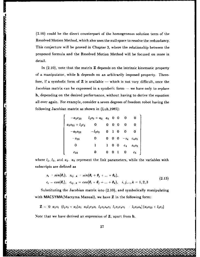
In (2.10), note that the matrix Z depends on the intrinsic kinematic property
of a manipulator, while h depends on an arbitrarily imposed property. There-
fore, if a symbolic form of Z is available - which is not very difficult, once the
Jacobian matrix can be expressed in a symbolic form - we have only to replace
h, depending on the desired performance, without having to derive the equation
all over again. For example, consider a seven degrees of freedom robot having the
following Jacobian matrix as shown in (Luh,1985):
-a 2c 23 12 S3 + a3 a3 0 0 0 0
a3 s 23 + 12C2 0 0 0 0 0 0
-a 3S2 3 -12C3 0 1 0 0 0
-S 23 0 0 0 0 -S 4 C4 5
0 1 1 00 c4 S4S5
C23 0 0 0 1 0 Cs
where 12, 13, and a 2 . a 3 represent the link parameters, while the variables with
subscripts are defined as
s, sin(O ), s j .. , n(O, + Oj + ... + Ok), (2.13)
C,- cos(O,), c,.k cos( , O + ... + +k) i,j,..,k = 1,2,3
Substituting the Jacobian matrix into (2.10), and symbolically manipulating
with MACSYMA(Macsyma Manual), we have Z in the following form:
Z N 0 a 3 85 (12S3 -r a3 )Sn a312C3S5 1283S4C5 1283C4 ";5 - 12Sep4s (a3s23 + 12C2)
Note that we have derived an expression of Z, apart from h.
27
4l l16
In (2.10), any criteria function may be used, as long as the function can be
reduced to an expression in terms of joint variables only. For instance, consider the
following criteria function, H(9), for the obstacle avoidance problem(Nakamura, 1985)2:
H - ko W /{Co(xi) - 1} + ki Ij 1/(02, - , (2.14)i=l 1=1
where ko and kj are scaling factors; xi = (x1i, X2i, X3 )T is the position of the i-th
point among I points on the manipulator; 0),,. is the limit of j-th joint; and the
model of the obstacle in the workspace, Co(xi), is defined as,
Co(X,) =- Zkc y (2.15)k=1 "
where xk,rk, and s are the center coordinate, radii, and roundness exponent
of the obstacle object. Note that we can reduce H to a function of 0 only, by
transforming x, into f,(O) using (2.1), and thus can apply (2.10) to it.
2.4 Computational Consideration
In this section, an analysis will be made with regard to the computational effort
required to solve (2.11). Much of the analysis is based on the various results of
the research on computational efforts. So one can find more detailed discussions
in the references cited in this subsection.
For the sake of generality, we consider the general manipulator without any
special geometry, thus assuming that J and Z are not given in the symbolic form.
A special geometry that allows the symbolic form, of course, would enable much
more efficient computations.
The computational effort will be measured in terms of arithmetic operations
such as addition, subtraction, multiplication, and division. Furthermore, we as-
sume that the four arithmetic operations require approximately the same amount
21.ie problem wais originllly tIeated ii the dynantic co.text by using a potential function.
28
4
10 U
'0
of computation time, and the effort required to evaluate trigonometric functions
is negligible as compared to the total computational effort.
2.4.1 Motion strategy
In order to compute the joint trajectory for a given Cartesian path, We need.
briefly speaking, to take the following procedures: we first determine via points
on the path; then obtain, by using inverse kinematic methods, corresponding
points in the joint space; and finally concatenate these angles to generated the
joint trajectory.
How to generate the via points, and how to determine an appropriate number
of the points are important subjects in the motion planning area. Too many via
points result in a wasteful computation and slow motion, whereas too few result
in inaccurate trajectory control. In addition to deciding the via points, how to
generate intermediate points between the via points is another important issue.
Usually interpolation methods are used to generate intermediate points, which
we will call knot points.
When obtaining joint values corresponding to a via point, we use iterative
methods if a symbolic solution is not available. So, determining joint angles for a
via point involves a number of iteration steps; each step in turn requires a series of
computations. Hence, the total computational effort, Ntoata, required for a given
trajectory is obtained in general as the following:
Ntota= Neo, + N'k=
Nk Nite .aionNep
where Nco,, is the computational effort for concatenating knot points either in
workspace or joint space, Ne,, the number of via points, Nk the computational
effort for inverse kinematics at each point, Nert,,n the number of iterations at
29
Lam0I
the point, and N,tp the computational effort at each iteration step. Assuming
that, as compared to the other term in Nt,,tI, Neon is relatively small, we will only
discuss each of remaining terms, in a reverse order.
2.4.2 Computational Effort at Each Iteration Step
If (2.11) is to be solved numerically, the computational effort at each iteration
step, Ntep(or N, in this case), is evaluated as follows:
N, = NFK + Nj 4- Nh + N,.1 (2.16)
where NFK denotes the computational effort required for the forward kinematics,
(2.1), Ni the effort to obtain the Jacobian matrix, Nzh for Zh in (2.10), and N,.t.
the effort needed by the numerical method for solving the system of nonlinear
equations.
For the general manipulator with revolute joints - no significant difference
is expected when a few prismatic joints are included - NFK is given as (Ange-
les,1985)
NFK = NR + NT (2.17)
NR = 36(n- 1) 4; NT = 16(n- 1) +2
where NR and NT indicate the computational efforts required to compute orien-
tation and position of the end effector'.
Nj for the general manipulator, with Waldron's scheme, is given as (Orin,1984)
Nj - 45n - 93 (2.18)
Since we have not, at this point, chosen a specific criteria function from a variety
of choices, let us simply assume that we have derived h with relatively a small
3 We derived these general formula on the hasis of the computation algorithm in (Angeles,1985).
Slightly different formula can result depending on different computation details
030
amount of computation as compared to the other parts of computation. If we
assume at the same time that a symbolic form of Z is not available, Zh in (2.10) is
more efficiently computed by first solving for A in (2.7) with Gaussian eliminatior,
and then substituting it as in (2.8). Thus, Nzh is given as follows:
Nzh = NG + N,
N +3 "2 N, = (n- m)(2m-1) (2.19)-3 -2 6'
where NG is the effort for Gaussian elimination(Nakamura,1985), and N, is that
for the substitution.
If we use, for example, MINPACK-1, one of the well-known software packages,
to solve the system of nonlinear equations, the computational effort, N,.,, becomes
(MINPACK Manual)
, .i = 11.5n 2
This package, by the way, is primarily based on an improved version of Powell's
hybrid method, a method that combines the Newton-Raphson method with the
steepest descent method (MINPACK Manual).
Consequently, the total effort of computation for the general manipulator with
kinematic redundancy per iteration for the proposed method becomes as follows:
N, = m3 + 11.5n2 - - - + 96n - 139 (2.20)3 2 6
As an example to show the total computational effort as well as the relative
significance of each part in it in a realistic situation, let us evaluate the effort when
n = 7 and m = 6. According to aforementioned estimations, we have N, = 1306,
in which, NFK = 318, Nj = 222, Nzh = 202, N,,i = 564.
2.4.3 Number of Iterations
The number of iterations required for a system of nonlinear equations depends on
several factors. Among these, there are some major ones such as the initial esti-
mate of solution, the particular updating algorithm being used, and the distance
of the estimate at the present step from singularities.
In the inverse kinematic context when the end effector is successively passing
adjacent points, the initial estimates are usually good enough to use such a fast
converging algorithm as the Newton-Raphson method. For applications with
poor initial estimates, however, we need some correctional algorithms such as
the steepest descent method. Alternatively, we may use a method that combines
the Newton-Raphson method and steepest descent method, such as the Powell's
hybrid method mentioned in the previous subsection.
With the Powell's method, solving a system of nonlinear equations that con-
* sists of trigonometric functions - thus very similar to the kinematic equations
- is reported to require from about 12 to 15 iterations for systems of up to nine
equations(Rabinowitz,1970). This data shows a good agreement with the result
by Benhabib et al(1986), which reports that the number of iterations for seven
degrees of freedom redundant manipulators is less than 15.
2.4.4 Minimum Number of Via Points
One extreme approach to control the motion of the end effector is to obtain joint
solutions at every sample interval. Obviously it requires considerable amount of
real time computation. One possible way to improve the approach is to compute
the joint solutions at every kth interval and then to interpolate on joint angles
(Taylor,1979). The difficulty with this way is that the number k that guarantees
a certain deviations, when interpolation is performed, from the desired path is
changing from point to point. So a fixed k small enough to ensure a given deviation
everywhere in the workspace requires still considerable amount of computation.
Another approach (Benhabib,1986) is to precompute joint solutions for suf-
ficiently large amount of via points in the Cartesian coordinates off-line, and to
32
0N( #
interpolate joint angles on-line. This approach may also waste computations and
storages, since this sufficient amount is not the same everywhere. In addition,
this approach requires us to know the path and corresponding via points well in
advance, so that we might execute the motion without much delay.
Then there follows a natural question: What is the number of via points
that is minimal yet guarantee a given deviation? An effective solution to this
question is found in Taylor's algorithm called Bounded Deviation Joint Path (
Taylor,1979). This algorithm computes, for a given straight line segments in
Cartesian coordinates, nearly minimal number of via points and corresponding
joint solutions, in a recursive way.
This algorithm requires one of inverse kinematic methods. Furthermore, it ap-
pears to require, if not explicit, a fixed transformation from the Cartesian space
to joint space. As we will show in the following chapters, the proposed formula
with the kinematic equation has the property of the fixed transformation. There-
fore this useful algorithm is expected to help the proposed formula efficiently and
accurately control kinematically redundant manipulators. We list the algorithm
in Appendix 1. In Chapter 4, we test the algorithm in conjunction with the
proposed formula.
On the other hand, there has not been, to our knowledge, any application
of the algorithm to the kinematically redundant case. In this sense, the appli-
cation of the algorithm may be considered an extension of the algorithm to the
kinematically redundant case.
2.5 Comparison with Other Methods
In this section, the proposed formula corresponding to equation (2.10) will be
compared with two existing null space expressions: the expression used by Luh
:3
011?
and Gu and the extended Jacobian method. The relationships will be investigated
on the basis of these comparisons.
2.5.1 Relationship with Luh's Expression
Luh and Gu (Luh,1985) proposed a null space matrix which is defined as
SN, = (n, '" n,)
where ns (i 7- 1,2..--, n - m) are orthogonal to every row vector of the Jacobian
matrix, so that for each n,, Jn, = 0.
Comparing this equation with (2.12), we see immediately that N, is a generic
* form of ZT; or conversely, Z' is a specific expression of N,. Since how to find N,
was not given, the formulation of Z in (2.9) provides with a systematic mean to
determine N,.
2.5.2 Relationship with Extended Jacobian Method
Baillieul, in the process of deriving a rate equation called the extended Jacobian
Method, presented another method to resolve the redundancy, also at the inverse
kinematic level (Bailleu1,1985,1986). This method derives the additional con-
straints by using the orthogonality characteristics between the gradient vector of
the criteria function and the null space matrix of J at the optimum, as
(I - J+J)h = 0 (2.21)
where J is the pseudoinverse of J as mentioned before.
From the resulting fully specified system of equations, one derives the new
Jacobian matrix, called the extended Jacobian, by partially differentiating with
respect to the joint variables, just in the same way as in the nonredundant case.
34
J0lill 1 11111F l
LUF
Among the n scalar equations in (2.21), only n - m equations are independent
constraints to be determined; for the rank of the null space matrix is n - m. The
detailed procedures of determining the n - m constraints and their concrete func-
tional forms are not known yet, except for the case n m + 1. When n m + 1,
that is, for the manipulator with just one redundant degree of freedom, a con-
straint is derived, through a series of procedures, as the following (Baillieul,1985)
G() njh (2.22)
=0
where
nj = ( IA 2 , .., ,") T (2.23)zA, = (-1)'+ det(P , J2, ..IJ -1 1 +1 1_1,in )
where det(.) is the determinant, with jk the k-th column vector of the Jacobian
matrix.
It is shown in Appendix 2 that (2.10) reduces to (2.22) in the case that n
m + 1. Considering this fact and that Z in (2.10) is a null space matrix of rank
n - m, we may regard (2.10) as a concrete expression of n - m independent
constraints.
2.6 Conclusion
To sum up, we have obtained a closed-form formula for the inverse kinematics
of redundant manipulators. It was demonstrated that the proposed formula is
concise in form, general in application, and easy to include the desired perfor-
mance. It was shown that the matrix, Z, in the formula consists of a set of the
* basis vectors of the null space of the Jacobian matrix. The comparison of the for-
mula to the other methods shows that the formulation provides with a systematic
mean to obtain Luh's null space matrix and that the formula serves as a concrete
expression for the general case of Baillieul's formulation. Whether the formula is
35
S%
U- F' ~ -, ~ ~U%

effective as a kinematic control method will be tested in experiments in Chapter
4.
36
I0
Chapter 3
Relationship with ResolvedMotion Method
3.1 Introduction
In Chapter 2. we proposed a formula that resolves the kinematic redundancy
at the inverse kinematic level, by using the null space. The similarity of the
formula to the null space term of the Resolved Motion Method led to a conjecture
that the former may be the counterpart of the latter at the inverse kinematic
level. In this Chapter, we will investigate their relationship and try to prove
that the conjecture is correct. Not only for that, we will also derive from the
proposed formula the counterpart at the differential level. In addition, we will
compare the numerical efficiencies of the two methods, too. In conjunction to
the comparison, we will discuss the repeatability problem in the Resolved Motion
Method, which was pointed out in (Baillieul,1985; Klein,1983), and examine if
the proposed formula solves it.
37
4
° ]
3.2 Resolved Motion Method
In this section, we first introduce the Resolved Motion Method for the redundant
case and review its characteristics. Then the causes of repeatability problem in
this method will be analyzed.
3.2.1 The Method and Its characteristics
The kinematic equation for manipulators given in (2.1) is again,
x - f(0) (3.1)
* where x is an m-dimensional vector representing the location of the end effector
with respect to the base coordinate system in the workspace, 0 is n-dimensional
vector representing joint variables, and f is a vector function consisting of m
scalar functions.
As mentioned in Section 1.1.1, the Resolved Motion Method first derives the
differential relationship by differentiating the kinematic equation with respect to
time as
*=Ji (3.2)
where the Jacobian matrix J defined as J is an m x n matrix (Whit-
ney,1972). T hen by inverting the matrix, we obtain the joint velocity, 9. For the
nonredundant case(n m), J being square, we can have 9 as
9 = J-x.
*. For the redundant case, however, since n > m, J does not exist. Instead,
we use a generalized inverse, J+, as (Ben-Israel and Greville, 1980),
-* (3.3)
38
0 'A1 ,
where J+ is defined as
j+ = jT(jjT)-I. (3.4)
This matrix, known as Moore-Penrose pseudoinverse, has by the way the following
properties:JJ+J = J
J+JJ+ = J+
(j+J)T =j+j
(jj+)T = jj+
The most general solution to (3.2) is known to be (Ben-Israel,1980)
= J+i + a(I - J+J)h (3.5)
where (I - J+J) is the null space of J, with a a gain constant, and h an arbitrary
vector. Equation (3.5) gives a way to resolve the redundancy at the velocity level.
We may call the first term in the r.h.s. a special solution, and the second term a
homogeneous solution.
Lidgeois(Lidgeois,1977) developed a formulation of resolution of redundancy,
such that a scalar criteria function may be minimized, by setting to the vector h
the gradient vector of the criteria function, H as in (2.5). He expresses (3.5) in
terms of the infinitesimal displacement, as
df = J+dx + a(I - J+J)h (3.6)
6 = adt
In (3.6)(or (3.5)), at time t, the special solution first moves the end effector to a
location x(t). Then, the homogeneous solution, on the other hand, forces joints
* to have self-motion to achieve an equilibrium (or optimum), 0', where H has a
local minimum, for x(t). In practice, however, it takes a certain amount of time,
6t, for the joint variables to reach 0', when the end effector has already moved
to a new location, x(t + 6t) -- thus requiring a new 9 . Therefore, the joint
39
'III Id I II II III V 1,1 111 P , III
variables never reach the optimal configuration, but continuously trail behind
with a slight difference in the direction of the end effector displacement, dx. In
other words, if the end effector would stay at a location sufficiently long, the
joints could eventually ,chieve the optimal configuration corresponding to that
location. This analysis appears helpful for understanding the following problem.
3.2.2 Repeatability Problem
The repeatability in the robotics context may be defined as the ability to give
the same joint values for a given location in workspace, regardless of the path of
end effector to that location. In mathematical terms, the repeatability means the
fixed transformation from the workspace to joint space. The lack of repeatability,
of course, can be a considerable drawback in robot manipulators which perform
cyclic tasks, because, as the end effector traces the cyclic path, joint variables
evolve into states which cannot be predicted in advance.
Klein and Huang (Klein and Huang,1983) noted this problem in (3.3), the
Resolved Motion Method without null space term. Baillieul mentioned the same
problem in (3.6), the method with null space term (Baillieul,1985). Then what
would be exactly the reason for this problem? The above analysis on the charac-
teristics of the method may help understand the reason.
More specifically, the analysis implies that the problem is caused by the fol-
lowing two factors:
1. Because of the directionality of dx in the special solution, the joint variables
have different values depending on the direction of the repeated path -
6 for instance, a cyclic path - in the workspace. Note, however, that the
repeatability can be preserved when tracing only one direction of the cyclic
path even in the presence of this factor (Baillieul,1985).
40
6N
I
2. Because of the irreters:bilty of the homogeneous solution part, they never
return to the initial configuration, once the joint variables reach a steady
state trajectory near to the optimal trajectory, 9(t)'. This situation can
happen at the initial transient period when initially guessed joint values
are far from the optimum; for the optimal joint values cannot be known in
advance.
Beside these factors, as briefly mentioned in Section 1.1.3., another pattern
of repeatability problem can exist when, among the multiple joint configurations,
transition from one configuration to another happens. About this pattern of
repeatability, we will discuss more in detail later.
To sum up, our analysis on the characteristics and the repeatability problem of
the method may lead to a conclusion: if we stay in one kind of joint configuration,
and if we trace the equilibrium(or optimal) joint values 9 (t), then we can pre-
serve the repeatability. Then this conclusion, together with the aforementioned
conjecture between the two methods, brings about another question: What is
the relationship between the equilibrium states, 0(t), and the states that satisfy
Equation (2.11)? The following section gives the answer to this question.
3.3 Relationship between the Two Methods
In this section, we will investigate the relationship between the proposed formula
and the Resolved Motion Method. More specifically, we will try to give the
answer to the question raised in the previous section: the relationship between the
equilibrium states of the Resolved Motion Method and the solutions of Equation
(2.11). At the same time, we will derive a rate equation, or differential relationship
like the Resolved Motion Method, from Equation (2.11).
41
-J7, J U- "W
3.3.1 Equilibrium State
In the Resolved Motion Method expressed in (3.6), if the end effector stays at a
location sufficiently long, the joints arrive at the equilibrium, stopping the self-
motion. Hence we have dO = 0, in addition to dx = 0 - the condition for fixed
end effector location. Therefore, from (3.6) we have
(I - J+J)h : 0.
It is proved in Appendix 3 that this equation holds if and only if (2.10) holds; thus
the proposed formula is the necessary and sufficient condition to be satisfied when
(3.6) has converged to its equilibrium states. In other words, (2.11) gives the exact
O_ equilibrium state, the optimal joint configuration, at which (3.6) will eventually
arrive by self-motion for a fixed end effector location. Thus, we may regard (3.6)
in the Resolved Motion Method as an approximated equation linearized at states
that are exactly determined by (2.11). Note that the above equation is the same
as the extra set of constraints proposed by Baillieul (Baillieul,1986).
The practical implication of this relationship would be that we can obtain the
equilibrium joint values either by solving (2.11) or by making sufficient iteration
of null space term of Resolved Motion Method with fixed end effector location.
However, as mentioned in Section 1.1.1, Resolved Motion Method, being a rate
equation, is not self-starting: given a location of end effector, corresponding equi-
librium joint values cannot be determined without using other methods.
When approaching the equilibrium, the speed of convergence is determined by
the value of 6: the larger the value, the faster is the convergence. The value of
* a, however, has an upper-limit, above which the equation becomes numerically
unstable, not to mention that the manipulator cannot respond because of the
torque limitation.
* 42
3.3.2 Differential Relationship
The proposed formula and the kinematic equation, in contrast to the Resolved
Motion Method, are a set of state equations or equilibrium equations that maps
from one space to another. Yet, these equations have in themselves all the neces-
sary informations about motion such as velocity and acceleration. Then how do
we derive motion from these state equations? More specifically, how do we derive
the joint velocity from these equations?
This question, obviously, is practically important, because often we need to
know joint velocity beside joint displacement. For example, when the dynamic
control is needed, or when the motion is specified in terms of end effector velocity,
it is more convenient to obtain joint velocity, by using the differential relationship,
than to obtain joint displacement.
To derive the joint velocity from (2.11), we have at least two ways:
1. Differentiate the equation with respect to time. Then, the Kinematic equa-
tion part becomes the well known Jacobian equation, x = Ji, while the
second part becomes 0 = J,., where J,. = 3zh. Combining these, the
resulting equation becomes
where
Je [;J J,
Inverting the above equation gives the joint velocity. Here, J, is so called
the extended Jacobian matrix by Baillieul (Baillieul,1985,1986)
2. Since J is given, use the pseudoinverse method in (3.6).
43
0
The first way, although conceptually simple, turns out to be an inefficient
method, because J, is a very complicated matrix - see the expression in (Bail-
lieul,1985). In the second way, on the other hand, we need to evaluate J+ from
J, which requires a substantial computation effort - note that we cannot make
use of Z already obtained with another intensive computation.
Instead, we can derive joint velocity by using the following relationship, the
proof of which is in Appendix 5:
0
where 1, is the identity matrix of rank m and JE is defined as
JE [~](3.8)Then the null space matrix is determined as
' z jIJ+J = J-1 01 (3.9)
Z
Substituting these matrices into (3.6), we have
JE [Zhj (3.10)
By this way, we can make use of the already obtained Z, and thus saving compu-
tation time.
3.3.3 Summary
* The relationship between (2.11) and (3.6) may be clearly summarized in the fol-
lowing block diagram. The comparison of numerical efficiency for one iteration is
treated in the next section, whereas the overall computation efforts are compared
in Chapter 4 and Chapter 7.
44
001
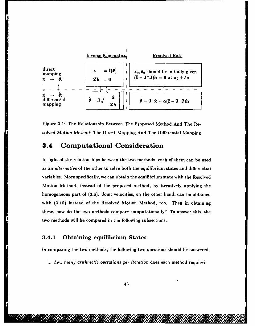
Inverse Kinematics, Resolved Rate
direct x = f(0) i x0, 00 should be initially givenmapping
x - 0 9: Zh =0 (I-J+J)h 0atx 0 +6x
differential JE1 =J* + a(I - J+J)hmapping Zh
Figure 3.1: The Relationship Between The Proposed Method And The Re-
solved Motion Method; The Direct Mapping And The Differential Mapping
3.4 Computational Consideration
In light of the relationships between the two methods, each of them can be used
as an alternative of the other to solve both the equilibrium states and differential
variables. More specifically, we can obtain the equilibrium state with the Resolved
Motion Method, instead of the proposed method, by iteratively applying the
homogeneous part of (3.6). Joint velocities, on the other hand, can be obtained
with (3.10) instead of the Resolved .Motion Method, too. Then in obtaining
these, how do the two methods compare computationally? To answer this, the
two methods will be compared in the following subsections.
3.4.1 Obtaining equilibrium States
In comparing the two methods, the following two questions should be answered:
1. how many arithmetic operations per iteration does each method require?
45
2. how many iterations are necessary for each method to achieve the same
degree of accuracy(and repeatability) from the same initial condition?
The former question will be briefly examined here by first evaluating the num-
ber of operations per iteration for the Resolved Motion Method, and then com-
paring it with that for the proposed method already obtained before. The latter,
on the other hand, was partly answered in Section 2.4.4 for the proposed method.
Yet since the number of iterations for Resolved Motion Method is not known, the
complete answer can be made through a computation example for a special case
in the following chapter.
As in Chapter 2, it is assumed that the numerical value h is provided at each
iteration step with relatively small amount of computation.
The computational effort, N1 , required for the proposed method at each iter-
ation step was obtained in (2.20) as
23 mN, = -m -t 1.5n + 2nrm--- + 96n - 133
3 2 6
On the other hand, the total computational effort required for the Resolved Mo-
tion Method, X2, at each iteration step or integration step, may be expressed
as
N2 = Ne(Nj + N.) + Nb (3.11)
where Nj is the effort required to compute the Jacobian matrix; N., the effort
required to evaluate the r.h.s of (3.6), once the Jacobian matrix is given; and
N , the number of times of evaluations of (3.6); Nb, the effort for numerical
integrations. For the general manipulator, Nj is given in (2.18) as
N = 45n - 93 (3.12)
and N is evaluated in (Nakamura,1985a) as,
N. 2m -+nm 2 5nm+ -n (3.13)
46
N,,,, together with Nh, depends on the specific numerical integration method to
be used. For example, fourth-order Runge-Kutta method requires that Nv = 4
and Nb = 13n; while most predictor-corrector methods require that N, = 2 and
Nb = 23n(Hamming,1973). Considering that N 2 heavily depends on the sum of
N,, and Nj, the latter method is much more efficient.
Therefore, N2 with the predictor-corrector method, is given as
_~ m nn z +ln r 2 +ll 4N 2 = - -,2nM2-+1nm+2M 2
+ll1- -m- 186 (3.14)3 3
On the other hand, Runge-Kutta method requires
N 2 = m 3 + 4nm 2 + 2Onm + 4m 2 + 189n - 8m - 372 (3.15)
When n =- 7 and m = 6, N2 = 1867 for the predictor-corrector method and N2
3503 for Runge-Kutta method, while N, = 1306 again. In this comparison, we see
that, if the predictor-corrector methods are used for the numerical integration,
the Resolved Motion Method requires about 43% more computational effort than
the proposed method per iteration, when n = 7 and m = 6.
3.4.2 Obtaining Joint Velocity
The comparison of computational efficiency of the two differential relationships
is quite straightforward: the only differences are the integrands in the r.h.s. of
(3.6) and (3.10). Therefore we have only to compare the computational efforts
for these terms; the remaining terms are exactly the same.
For the Resolved Motion Method, the effort for the terms, N, is again,
N 2 2m 3 +nm 2 + 5nm + m2 2m n
*3 3
Meanwhile, for (3.10), the corresponding part denoted, Nj,, is obtained as
follows:
N,, = Nz± + NG, (3.16)
47
N
where Nzh is the effort required to compute Zh, and N(, is the effort for Gaussian
elimination when inverting JE. Nzh was evaluated in (2.19), which is again
Nzh = NC + N,
N( =2, + . .N, = (n- m)(2m- 1)3 2 C ,
where Nr is the effort for Gaussian elimination(Nakamura.]l&Wa), and N8 is that
for the substitution of Lagrangian multiplier.
Meanwhile, N.,0 is obtained simply by substituting m for n in NG-, resulting
in
Ncn 2n 3n 2 7n3 2 6
Hence, Nj, becomes
2n 3 3n 2 13n 2m 3 m 2 m'V_ I= _ -- - - -- + 2rim (3.17)
3 2 6 3 2 6
The total computational effort N 3 for (3.17) was initially given as
N 3 = N.,(N, + N,,) + N
Assuming that the predictor-corrector method is used, and substituting for Nj
and Nb respectively, N 3 becomes
4n 3 5 4m 3 2 m,V 3 + 3n 2 -107-n+ -- 3+4nm-186 (3.18)
3 3 3 3
Again when n = 7 and m = 6, N 3 = 1597, as compared to N 2 = 1867, requiring
about 15% less computational effort.
3.5 Conclusion
Summing up, we have introduced the Resolved Motion Method and observed that
the deviation from equilibrium states is due to linear approximation characteris-
tics. The repeatability problem was analyzed on the basis of this understanding.
48
0I

We concluded that the proposed formula provides with equilibrium states that
preserve the repeatability. The equilibrium states are also the states at which the
Resolved Motion Method is considered as a linearized equation. In addition, the
differential relationship was derived from the proposed formula. The computation
efforts for one iteration with the two method were compared.
49
0m-
Chapter 4
Numerical Experiment onKinematic Control Methods
4.1 Introduction
In Chapter 2, we have derived a closed-form formula for inverse kinematics of
kinematically redundant manipulators that can achieve additional performances
represented in the performance measures. In Chapter 3, we have investigated on
the relationship between the formula and the Resolved Motion Method, focusing
on the repeatability problem. Although most of the results obtained appear rather
obvious, some important points had better be verified through experiments.
In this chapter, therefore, we will make numerical experiments or simulations
to confirm some of the important results. To this end, we select a kinematically
redundant manipulator and apply (2.10). The resulting system of equations is
solved numerically for x(t), the end effector location. In parallel to using (2.11),
the Resolved Motion Method method is applied to the same manipulator with the
same tip motion. The points we try to examine or verify through the simulation
are as follows:
50
6I
1. Whether the resulting system in (2.11) gives kinematically correct joint
variables for a given x, achieving the additional performance represented
by the criteria function we select.
2. How the present method compares to the Resolved Motion Method in terms
of accuracy, repeatability, and computational efficiency.
3. Whether the present method gives, in fact, the same equilibrium states as
the Resolved Motion Method will eventually reach.
In the comparison of computational efficiency, we consider two situations:
when solving the steady state equilibrium states with fixed tip location, and
when obtaining joint trajectories with tip moving along the Cartesian path.
4.2 System Description
We use the same manipulator presented in the paper (Yoshikawa,1984) for the
sake of comparison with data obtained in that paper: a 3 degrees of freedom
manipulator with the end effector moving in the (z, y) plane; thus kirematically
redundant. The schematic diagram with necessary parameters is in Figure 4.1.
The desired performance is to avoid singularity. A good criteria function for
this objective may be the manipulability(Yoshikawa,1984,1985a), which is given
asI
H = det(JJT) (4.1)
The kinematic equation is given as
X = 1181 + 12812 + 138123 (4.2)
Y = l1 cI + 12c12 + 13cI23
51
II 11 v 1 1. 1AI 1
*% A -IZM EJ
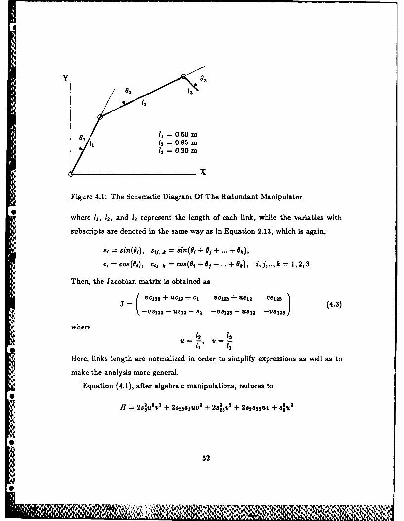
y
11 = 0.60 m1= 0.85 m
13 = 0.20 m
x
Figure 4.1: The Schematic Diagram Of The Redundant Manipulator
6 where 11, 12, and 13 represent the length of each link, while the variables with
subscripts are denoted in the same way as in Equation 2.13, which is again,
si= sin(e,), 8j j...kh = sin(Oj + 9, + ... + 0k)?
C= cos(0,), cj,...jk= eo.(9,+89,+ ... + 9), i,j, ..,k =1,2,3
Then, the Jacobian matrix is obtained as
VC 1 2 3 + ULC12 + C1 VC1 2 3 + UC12 VIC123 (43(-VS12S - U8S12 - 81 -VS12 3 -UtL 12 -VS123 J
where12 131 , l11
Here, links length are normalized in order to simplify expressions as well as to
make the analysis more general.
Equation (4.1), after algebraic manipulations, reduces to
2a H U 2v 2 + 282333UV +23 3sV2 + 282 82 3UV + 2 U2
52
By partially differentiating, we obtain the gradient vector, h = (hi, h2 , h 3 )T, with
h, =0
h 2 = 2(C2 ssaU + 82233)v2 + 23223uv + 822u2
h3 = 2(SssU2 + 823SU + 8223)v 2 + 2C23 2Uv
Meanwhile, (2.9) is simplified to,
Z = [s3uv - Ssuv - 823V 823V + S2u]
By applying (2.10), we get
2u~v(s 2sss3 - C238) + uvs(232 3 2s 33 - 3822338s) + 2svS 2833+
uv'(C33 - C22) + 2uv'(s 2 s2233 - c22 3 ) - u V322s 3 - 2usVs233 (4.4)
=0
where the same definition as in (4.2) is used for the subscripts.
The system of equations, (4.2), and (4.4) now fully specify the originally under-
determined system of equations, (4.2), while maximizing the criteria H in (4.1).
The system of equations may be solved either purely numerically, or by symbol-
ically reducing variables - in this example, 01 - and then by using numerical
methods. Incidentally, this example suggests that it is possible to reduce vari-
ables, thus reducing the order of the system of nonlinear equations, after resolving
the redundancy first with all the joint variables.
4.3 Procedures
The task is to trace a square path - thus a cyclic path. As shown in Figure 4.3,
* the z-y coordinates of the four vertices of the command path in the workspace
are successively given counterclockwise from the upper-left vertex as follows:
(446.00, 91.514),(446.00,-8.486), (546.00,-8.486),(546.00, 91.514),
where the units are mm.
53
4
The system of equations were numerically solved for joint values, with regard
to consecutive equidistant points on the command path - in this example, 100
segments each side - in the counterclockwise direction. As mentioned before,
the MINPACK-1 subroutine was used to solve the system of nonlinear equations.
The subroutine, by the way, allows only one set of local solutions, among multiple
sets of solutions.
Meanwhile, the Resolved Motion Method in (3.5) is also applied to this ex-
ample for the same path, which the end effector is to track with a constant
speed of 10mm/sec. (3.5), a system of differential equations, was solved with
the fourth order Runge-Kutta integration method, together with the LINPACK
subroutines, with the integration time step size, At = 0.01 seconds. We can also
use the predictor-corrector method for the better efficiency at the cost of the non
self-starting disadvantage and more complex program.
The simulation for the Resolved Motion Method was made with initial joint
angle values of (-40.5006, 141.6408, 78.4169) in degrees, which are far from equi-
librium states, that were deliberately selected to examine repeatability. The same
initial value was also used as the initial guess for the above nonlinear equations
for fair comparison of the two methods.
In addition to tracking the square path, another path was traced in order to
compare the efficiency in the case when obtaining the joint trajectory is required.
The path tried is a straight line path connecting z = 0.1m, y = Om and z =
1.6m, y = Om, along which the tip reciprocates. The proposed formula is used
to obtain joint angles corresponding to the via points determined with Taylor's
algorithm mentioned in Section 2.4.4. The via points of the Resolved Motion
* _Method, on the other hand, are simply the equidistant points determined by line
segments(the constant tip speed multiplied by the integration time step). Thus,
with this method, the equidistant via points are determined either by varying tip
54
i',,54
speed or the integration time step. For the proposed formula, hence, the deviation
is automatically bounded within a specified value, whereas for the other method
the the deviation is controlled by varying the tip speed or time step with trial
and error.
4.4 Results
The numerical results of simulations are plotted and listed in Figure 4.2, 4.3 and
Tables 4.1, 4.2, 4.3:
" Figure 4.2 is the plot of joint variables solved with the two methods. Note
that the 3-D trajectory of joint variables is represented with two 2-D plots:
01 vs. 02 and 01 vs. 03.
* On the other hand, Figure 4.3 shows actual trajectories, with the two meth-
ods, of the end effector in the workspace, as compared to the command
path. The actual trajectory was determined by forward kinematics with
joint values obtained by each method.
* Figure 4.4 shows the accuracy and corresponding computational effort to
achieve it, with the two methods. The task is to reciprocate a horizontal
straight line. Again, the proposed formula was used in conjunction with
Taylor's algorithm. Since the Resolved Motion Method may be viewed as
a one-time iteration method, the iteration number for this method in the
figure is in fact the number of integration steps required to cover a given
line-segment.
* Table 4.1 enables one to numerically compare the accuracy of the tip loca-
tion, and observe the irreversibility factor due to the homogeneous solution
term of (3.6), at the transient period. For the purposes, we have selected,
55
from the data in Figures 4.2, 4.3, five sets of data, which correspond to
the consecutive vertices of the square path - counterclockwise from the
upper-left one, when the tip begins to trace at the very first cycle.
Table 4.2 shows the comparison of the accuracy and repeatability when
tracing opposite directions in the steady state. In order to obtain the data,
the tip was made to reciprocate a straight line segment, which was set to the
left vertical side of the square path, after the first two cycles of the square
path, when the transient effect appeared negligible.
" Table 4.3 verifies the relationship proved in Appendix 2: the solution with
the Resolved Motion Method becomes equal to that with the proposed
method after sufficient time, provided that dx = 0. The four vertices were
selected for the comparison, as in Table 4.1. To obtain the data with the
Resolved Motion Method, the tip was commanded to stop at each vertex,
where it made the self motion through iterations of the homogeneous term
of (3.6), until the joints converged to an equilibrium configuration. At each
vertex, about 25 iterations were needed to converge to the joint values ob-
tained with the proposed method, within the accuracy of 10 - 4 in degree,
with 6 = 10, which provides about the upper-limit speed of convergence
without causing numerical instability.
56
01P 1- 1
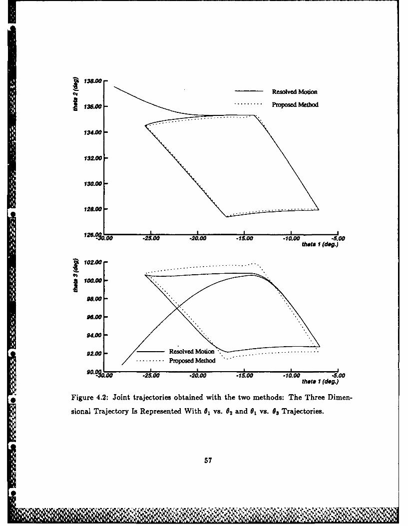
13800-
Resolved Motion
S134.00-
132.00-
132.00-
130.00- .....
128.001 ___
%10*2500 -20.00 -15.00 -10.00 -5.00theta 1 (dog.)
S102.00-
a100.00-
98.00-
96.00-
94.00-
92.00- Resolved Motion ................
00.0.00 -25S. 00 -20.00 -15.00 -10.00 -5.00theta I (dog.)
* Figure 4.2: Joint trajectories obtained with the two methods: The Three Dimen-
sional Trajectory Is Represented With 01 vs. 02 and 01 vs. 03 Trajectories.
57
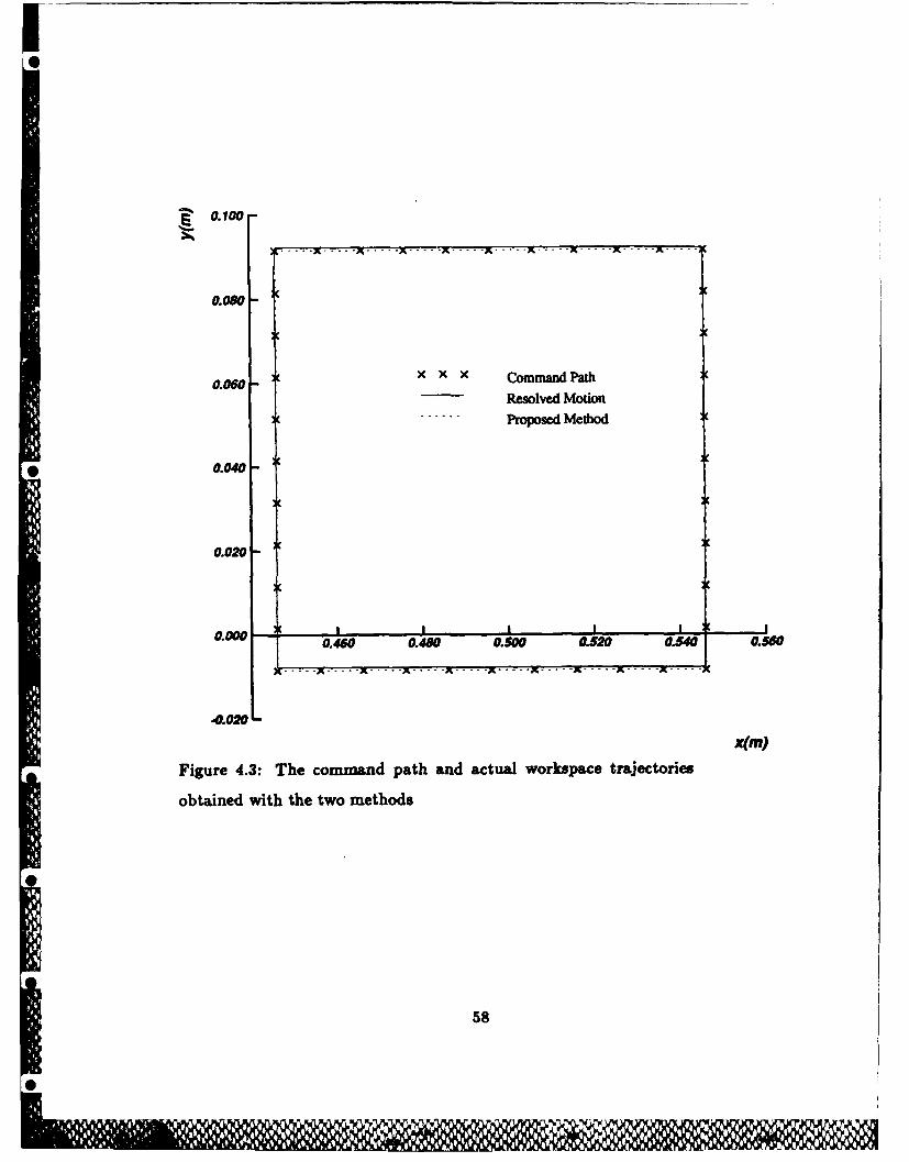
0.100
0.080-
0.060- X X X Comnmand PathResolved MotionkProposed Method
*0.040-i
0.020-
.00- X0.460 0.480 0.50 0.520 0.54 0.560
Figure 4.3: The command path and actual workspace trajectories
obtained with the two methods
58
QRS1II
'Pit,~
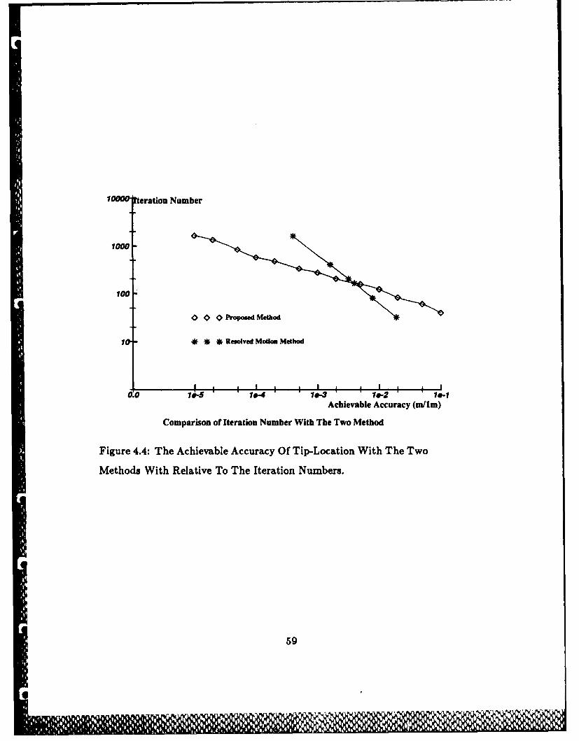
100 otration Number
1000-
100
C Propoed Method
1 * **Resolved MotionMethod
0.0 1~p 1 _&L4 1121 -Achievable Accuracy (mu1m)
Comparison of Iteration Number With The Two Method
Figure 4.4: The Achievable Accuracy Of Tip-Location With The Two
Methods With Relative To The Iteration Numbers.
59
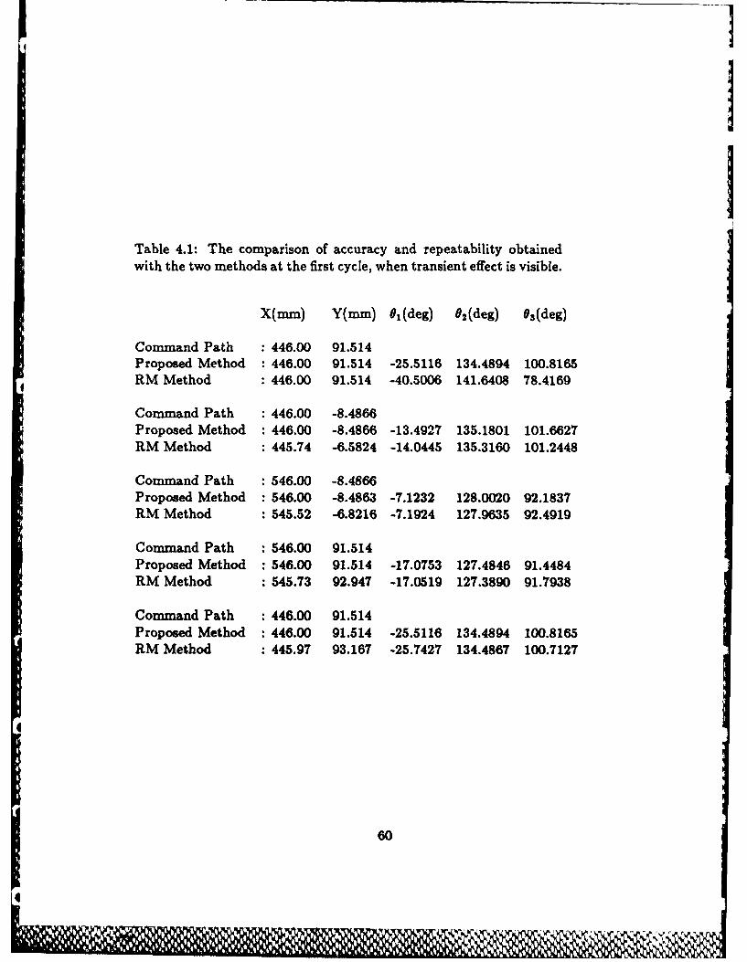
I~I;
I_
Table 4.1: The comparison of accuracy and repeatability obtainedwith the two methods at the first cycle, when transient effect is visible.
X(mm) Y(mm) 01(deg) 02(deg) 0s(deg)
Command Path : 446.00 91.514Proposed Method : 446.00 91.514 -25.5116 134.4894 100.8165RM Method : 446.00 91.514 -40.5006 141.6408 78.4169
Command Path : 446.00 -8.4866Proposed Method : 446.00 -8.4866 -13.4927 135.1801 101.6627RM Method : 445.74 -6.5824 -14.0445 135.3160 101.2448
Command Path : 546.00 -8.4866Proposed Method : 546.00 -8.4863 -7.1232 128.0020 92.1837RM Method : 545.52 -6.8216 -7.1924 127.9635 92.4919
Command Path : 546.00 91.514Proposed Method : 546.00 91.514 -17.0753 127.4846 91.4484RM Method : 545.73 92.947 -17.0519 127.3890 91.7938
Command Path : 446.00 91.514Proposed Method : 446.00 91.514 -25.5116 134.4894 100.8165RM Method : 445.97 93.167 -25.7427 134.4867 100.7127
4
60
IS lI 1' .'
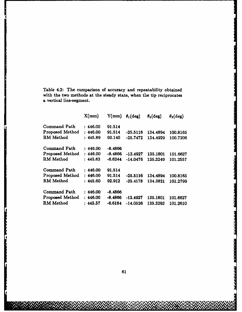
Table 4.2: The comparison of accuracy and repeatability obtainedwith the two methods at the steady state, when the tip reciprocatesa vertical line-segment.
X(mm) Y(mm) 01 (deg) 02 (deg) 0s(deg)
Command Path : 446.00 91.514Proposed Method : 446.00 91.514 -25.5116 134.4894 100.8165RM Method : 445.89 93.140 -25.7472 134.4929 100.7206
Command Path : 446.00 -8.4866Proposed Method : 446.00 -8.4866 -13.4927 135.1801 101.6627RM Method : 445.63 -6.6244 -14.0476 135.3249 101.2557
Command Path : 446.00 91.514Proposed Method : 446.00 91.514 -25.5116 134.4894 100.8165RM Method : 445.60 92.912 -25.4178 134.3821 101.2799
Command Path : 446.00 -8.4866Proposed Method : 446.00 -8.4866 -13.4927 135.1801 101.6627RM Method : 445.57 -6.6184 -14.0526 135.3293 101.2610
61
I
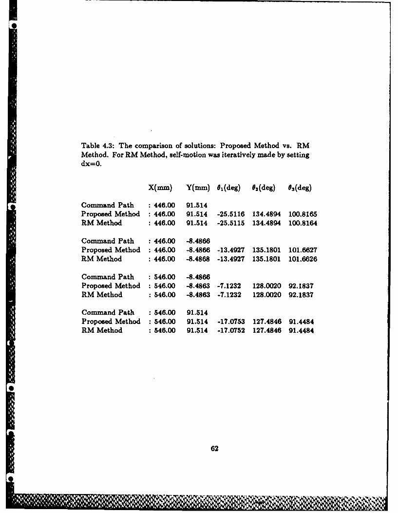
Table 4.3: The comparison of solutions: Proposed Method vs. RMMethod. For RM Method, self-motion was iteratively made by settingdx=O.
X(mm) Y(rnm) 01(deg) 0 2 (deg) 03(deg)
Command Path : 446.00 91.514Proposed Method : 446.00 91.514 -25.5116 134.4894 100.8165RM Method : 446.00 91.514 -25.5115 134.4894 100.8164
Command Path : 446.00 -8.4866Proposed Method : 446.00 -8.4866 -13.4927 135.1801 101.6627RM Method : 446.00 -8.4868 -13.4927 135.1801 101.6626
Command Path : 546.00 -8.4866Proposed Method : 546.00 -8.4863 -7.1232 128.0020 92.1837RM Method : 546.00 -8.4863 -7.1232 128.0020 92.1837
Command Path : 546.00 91.514Proposed Method : 546.00 91.514 -17.0753 127.4846 91.4484RM Method : 546.00 91.514 -17.0752 127.4846 91.4484
62
4.5 Discussions
From the results of simulations, we may evaluate the proposed method in terms
of accuracy and repeatability by comparing it with the Resolved Motion Method.
We can also derive some useful ideas from the relationship between the two meth-
ods.
Accuracy
As shown in Table 4.1 and Figure 4.3, the proposed method gives joint vari-
ables which exactly correspond to the commanded z and y, while maximizing
the criteria function to avoid singularities. Clearly, we see that the accuracy in6the workspace achieved with the proposed method is better than that with the
Resolved Motion Method.
Therefore, the proposed method provides useful means for accurate position
control of the end-effector, when the manipulator is kinematically redundant.
Repeatability
Table 4.2 and Figure 4.2 show that the repeatability is not preserved with the
Resolved Motion Method because of the two factors mentioned in Section 3.2.2:
the initial joint variables which are far from optimal joint values(Figure 4.2) and
the dependence on the direction, clockwise or counterclockwise, of the path to be
traced (Table 4.2).
On the other hand, it is obvious that the proposed method preserves the re-
peatability regardless of direction. In other words, the method provides a fixed
*- transformation from workspace to joint space. The property of fixed transfor-
mation is useful not only for the prediction of joint variables, but also for the
precomputation of position dependent terms such as the Jacobian matrix and the
63
pAlewM..
EL M~ -
0
inertia matrix (Raibert and Horn,1978).
Computational Effort
As mentioned before, the comparison of computational efficiency was made in two
situations: when solving the steady state equilibrium states with fixed tip loca-
tion, and when obtaining joint trajectories with tip moving along the Cartesian
path. The two cases will be discussed separately.
For Equilibrium State
The number of iterations to achieve the accuracy of 10 - 4 in degree by the proposed
method with MINPACK-1 is about from 10. On the other hand, the number of
*iterations required for the same accuracy by the Resolved Motion Method is about
25 1 - thus about 2.5 times more iterations than the proposed formula.
It is not immediately clear how the two method will compare for manipulators
with more degrees of freedom. Yet, we expect the Resolved Motion Method
would require a similarly larger computational effort than the proposed method,
considering the following factors:
As quoted in Section 2.4.3, the proposed formula requires about 15 iterations
for manipulators with up to none degrees of freedom. At the same time, it is
not quite probable that the Resolved Motion Method requires less iterations
for more degrees of freedom case;0
" Moreover the former requires about 43% more computation per iteration
than the latter.
For Trajectory Generation
'This number is based on the Runge-Kutta method. An efficient step-size control with the
predictor-corrector method may reduce the number of iterations.
64
J1
V.* , 0--
From the simulations, it turned out to be the deviation with the Resolved Mo-
tion Method is nearly proportional to the length of equidistant segments. This
length in turn is directly proportional to the number of integration steps, Natep,
or equivalently computational efforts. in other words, for a given straight line
segment, Ax, the number of integration steps, or iteration number, is estimated
as,Nate,,- IAxll
I116twhere x is the speed of the tip motion, 6t the integration time step, and 11.11represents the Euclidean norm of vectors. We can reduce, of course, Notp by
increasing the speed of tip motion and time step at the cost of accuracy and
numerical stability.
On the other hand, the deviation with the proposed formula, if Taylor's algo-
rithm is used, decreases exponentially with a base of 2 to 4 as the length between
two via points halves - by adding one via point in the middle. Figure 4.5 shows
the change of deviation as via points changes.
Thus, as Figure 4.4 shows, with sparse via points, the deviation resulting from
the Resolved Motion Method is smaller than that with the proposed method,
provided the same computational effort is applied. When the via points become
more than a certain number, the situation reverses. In the simulation, the break
point is when the number of via points for the proposed method becomes about
* 17, where the deviation is about 30mm, assuming total sum of lengths of links is
1M.
Since the proposed method requires about 9 iterations for a via point, the
total number of iterations is about 160. Hence, if the accuracy required is within
a deviation of less than 30mm per average link length of im, the proposed method
gives more accurate trajectory than the Resolved Motion Method.
In the case for more degrees of freedom manipulators, the comparison is ex-
65
.N
A.%
0*
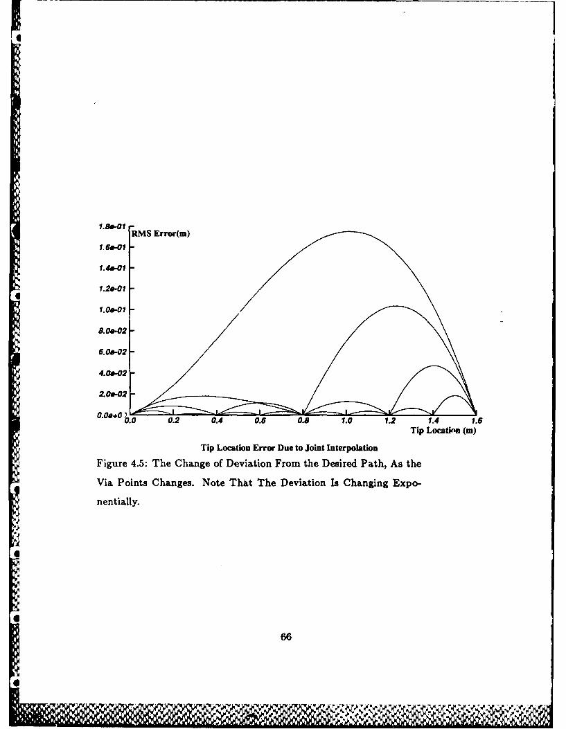
RMS Error(m)
1.6.-Cl
1.40-Cl-
1.2e-C1
1.00-01l
8. 0"-
6.0&-02-
4.0.-02-
2.0*-02
0 .0 0.2 0.4 0.6 0.8 1.0 1.2 1.4 1.6
Tip Location (in)
Tip Location Error Due to joint Interpolation
Figure 4.5: The Change of Deviation From the Desired Path, As the
Via Points Changes. Note That The Deviation Is Changing Expo-
nentially.
66
6r
-- - -- -
pected to be similar, because of almost the same reasonings made above, when
the equilibrium state case was considered.
Relationship between the Two Methods
The result in Table 4.3 shows a nearly perfect agreement of both solutions, ver-
ifying that (2.11) in tiLe proposed method is the equilibrium equation at which
(3.5) will finally arrive.
Because of the relationship between the two methods, we may use them in-
terchangeably as follows:
The exact equilibrium state can be determined either with the proposed
* method, or with the Resolved Motion Method by setting dx = 0. The latter,
however, would require more computations than the former, as discussed
before.
e The incremental displacement dl, which (3.5) of the Resolved Motion Method
easily provides, can be also obtained by using (3.10).
: .: 67
Chapter 5
Development of A DexterityIMeasure
5.1 Introduction
The benefits of using a quantitative measure in engineering systems are well
known. As mentioned in Section 1.1.3, a quantitative measure provide us with
a rational basis upon which we can, without having to rely on experience and
intuition alone, analyze, design, and control the systems.
In robot systems, too, various performance measures have been tried, which
were listed in Chapter 1. In the subsequent chapters, these measures, in a generic
form denoted as H, have been taken into account, when using kinematic control
methods for redundant manipulators.
In this chapter and next, we focus on a certain desired performance, dexterous
4t
configuration, and develop a corresponding measure, dexterity measure. This
performance, however, becomes in fact quite ambiguous unless the concept of
dexterity is more precisely defined. The concept of dexterity, when proposed byIKlein(1984), appeared to mean (I)the goodness of linear system of the differential
- 5o68
The beefitsof usng a uantittive easur in egineeigs yses rwl
relationship, as indicated by the determinant or condition number of the Jacobian
matrix; or (2)a natural appearance resulting from evenly distributed joint angles,
represented by summing the squares of the deviation of actuators displacements
from their midpoint.
According to this definition, the least dexterous configuration would be proba-
bly the singular configuration; for at singularity not only is the condition of linear
system at its worst, but also awkward appearances happen owing to lining-up or
folding of links. In this sense, therefore, dexterity may be viewed as a degree of
farness or distance from singularity. In the thesis, the meaning of dexterity is
explicitly specified as the distance from singularity.
S The distance from singularity, as mentioned in Section 1.1.3, may be repre-
sented with one of the following measures derived from the Jacobian matrix: the
determinant(or the manipulability measure for the redundant case), the condi-
tion number, and the singular values. Yet, in the case of redundant manipula-
tors, it was discussed that these measures cannot explicitly indicate the successive
changes in the degree of redundancy. This inability to indicate its change, consid-
ering that the degree of redundancy is an important constituent of the distance
from singularity, is an obvious shortcoming for distance measures. Furthermore,
even for a particular degree of redundancy, there appear relative differences in
the distance from singularity that have been unnoticed. Therefore, we feel that
a satisfactory dexterity measure should not only include the feature of indicating
the change in the degrees of redundancy, but also represent relative differences in
a particular degree of redundancy.
* In order to better understand the degree of redundancy and the relative dif-
ferences, we first review in Section 5.2, the concept of singularity, and some basic
knowledges about the degree of redundancy. Then, in Section 5.3, we derive a
new concept from observation of redundant manipulators. From this concept, a
69
-6 - - - -. ,%
II
new performance measure will be developed in Section 5.4. The property of this
measure will be discussed in Section 5.5. Finally some concluding remarks will
be made in Section 5.6.
5.2 Review of Singularity and Redundancy
This section presents reviews on two basic concepts, singularity and kinematic
redundancy, which are necessary for better understanding the distance from sin-
gularity in the redundant manipulators.
5.2.1 Singularity
Singularities can be easily observed by examining the differential relationship,
(3.2), which is again,
,i= (5.1)
where G is n-dimensional vector representing joint variables, x is m-dimensional
vector representing end effector location.
For the nonredundant case(n = m), the Jacobian matrix J is a square ma-
trix. When the Jacobian matrix becomes singular, a manipulator is said to be at
singular point.
Hence at singular point, the determinant of J, det(J) equals zero. This simple
fact. t-,%,, ther with the fact that the determinant is a continuous function of joint
variables, provides with some important insights:
1. When det(J) 0- 0, the rank of J being reduced, the arm loses corresponding
degrees of freedom, with the results that it cannot move in some directions
by' any combinations of small motions in the joints.
'Much of discussions here is based on the personal note on singularity by Professor B.K.P.
Hrn,,,, tile autlor' supervil.
70
X
2. Thus, as arm approaching this point, small movements in those directions
require very large displacements in joint space.
3. At singular points, since the determinant is a continuous function, its sign
changes. The change of sign, considering the determinant is the ratio of
differential volume of Cartesian coordinates to that of joint coordinates,
indicates a change from one kind of solution to another. In fact, just as
a change of sign in a continuous function cannot occur without passing
through zero, so the arm cannot change from one kind of solution to another
without passing through singularity. This property was also discussed in
(Uchiyama,1979)
4. At a singularity, thus, two different kinds of solution become one kind;
hence, the number of different solutions is reduced.
5. Items 3 and 4 can be explained in terms of Riemann sheets: multiple solu-
tions correspond to multiple sheets each of which represents the mapping
from joint angles to Cartesian coordinates; and singular points correspond
to the folds.
The first two items, by the way, may explain why keeping far from singularity is
closely related to dexterity.
From the fact that the determinant becomes zero at singularity, it functions in
a sense, as an indicator of the presence of a singular point. Besides, the absolute
value of the determinant, if geometrically interpreted, represents the volume of
parallelepiped made of n column vectors (or row vectors) of the Jacobian matrix.
This interpretation, together with the fact that at singularity the parallelepiped
collapses and the volume becomes zero, ;s in fact the basis of the idea that the
determinant is a measure of distance from singularity.
71
N
% 4~. N.- 'h
4
One disadvantage of using determinant, however, as an indicator of singular-
ity is that, once the rank of J is reduced, it does not distinguish between one
state of singularity and another although their remaining ranks are different; the
determinants of both of them are equally zero. The more accurate indicator for
this purpose would be probably the remaining rank, or degree of freedom, itself.
For redundant manipulators, it was pointed out in Section 1.1.3 that the
measure equivalent to det(J) is the manipulability measure, Vdet(JJT). Yet, this
measure, as mentioned in Section 5.1, cannot indicate the change in the degrees
of redundancy, which will be reviewed in the following subsection.
5.2.2 Kinematic Redundancy
The degree of redundancy r is formally defined as
r -n--rn (5.2)
where n is the degree of freedom, and mn the rank of workspace. In linear algebra
(Strang,1980), the degree of redundancy corresponds to the dimension of null
space of the Jacobian matrix, the degree of freedom to the dimension of its column
space, and the workspace rank to the dimension of its row space. In other words,
the degree of redundancy is the maximum number of linearly independent vectors
in the null space, e,, defined as
Jei 0 (5.3)
But, we find that this definition is not sufficient for describing the concept of
redundancy.
For instance, consider the following Jacobian matrix representing a three de-
grees of freedom planar redundant manipulator consisting of three two-dimensional
column vectors, P',JP, and JP as
j - (j' I 2 jIj 3 ).
72
1~Ir 'r W
% % %;N
%
If the second and the third links line up, that is J3 = cJ 2 with c any nonzero
constant, we know we do not have any redundancy left. However, the null space
vector that satisfies (5.3) is obtained as
e--(0 c -1),
which is a nonzero vector. Thus, according to the definition, the degree of redun-
dancy is one, whereas the observation indicates there is no redundancy. Then, how
can we explain this difference? The discrepancy can be resolved if we modify the
meaning of n in (5.2), as the available degrees of freedom. But, as mentioned in
Section 5.1, it turns out that this modified definition is still inadequate to describe
the relative differences in the distance within the same degree of redundancy.
5.3 A New Concept of Distance from Singular-
ity in Redundant Case
In this section, we will observe some Jacobian matrices of kinematically redundant
manipulators, and identify relative differences in the distance from singularity. On
the basis of the observations, we will propose a new definition of the distance from
singularity.
Again, the kinematic equation of a kinematically redundant manipulator is
generally given as follows:
x = f(O)
where x C Wm, and 0 E W" with with m < n. Then, tE<! Jacobian matrix from
the equation, which is given as J E Rmn, may be denoted in general as,
j = [j,, j2, .., y,, jm l-,.., jnl
where Jk is k-th column vector. If m linearly independent vectors are chosen,
without loss of generality, as the first m column vectors of J, then, from linear al-
73
.A
gebra, the remaining n - m vectors Jm- J,.., are linear combinations of J1 ,...,J"'
(Strang,1980).
Observations show that how many of these m vectors are included in the
linear combination for each of the remaining n - m vectors determines how far
from singularity a given configuration of the manipulator is at the moment.
To illustrate the point, let us select a manipulator with one degree of redun-
dancy, i.e., n - m - 1, where
j =jl,j 2 ,..jrnjn+l
Consider the following three cases of linear combinations for J,,+I:
1. jdm- = a1j 1
2. Jm-' = a1jl + a2 J2
3. Jn = a1j] + a2J2 -r ... + amJm
where a,'s, (i = 1,2,..,m) are arbitrary nonzero constants. What are then the
differences among these cases?
According to the formal definition in (5.2), the degrees of redundancy for the
three cases are the same, one. Alternatively, if the modified definition is used,
then the manipulator in Case 1 has no redundancy, whereas those in Cases 2 and
3 have equally one degree of redundancy. However, a careful observation reveals
that there still exists another difference in the distance from singularity between
Cases 2 and 3. The differences among the three cases may be explained as follows:
1. In Case 1, the manipulator gets into singularity, reducing its rank (< in), if
;any two of the first m column vectors happen to line up.
2. In Case 2, singularity arises if any two, except for J and 2 , of the m
column vectors line up.
74
%0%
3. In Case 3, it preserves its rank (= rn), although any two of the column
vectors happen to line up.
In other words, the chance for the manipulator to get into singularity decreases
by degrees, as the number of linearly independent vectors to be included in the
combination increases. These differences in chances of getting into singularity
make the relative differences, within the same degrees of redundancy, in the dis-
tance from singularity. Meanwhile, how many of J, j 2 ,..jm appear in each of
j,,l .. , jn uniquely determines the number of distinct combinations of rn lin-
early independent column vectors, or the number of distinct submatrices of rank
rn in the Jacobian matrix. Hence, this number of submatrices also represents the
margin from singularity; the larger the number, the less is the chance of getting
into singularity. Of course, the number reduces successively as the number of
lining-up of column vectors increases. Of the equivalent two, to determine the
number of submatrices would be much easier than to select rn vectors and to
examine how many of the rn vectors are included in the remaining n - rn vectors.
Note, at the same time, that the observation is not confined to this particular
example of one degree of redundancy case, but evidently true for general cases,
where the degree of redundancy is more than one.
As another example, consider the following five jointed robot having a three
dimensional workspace and thus two degrees of redundancy, where the Jacobian
matrix is given as,
J = (J1 j 2 j 3.14JSl
where J,'s are again the three dimensional column vectors. If Ji, J 2 ,and JP are
selected as linearly independent vectors, then j 4 and J5 are, in general, repre-
sented as
j4 = cIJ + c 2 j 2 -- c 3 j 3
J d1J' + d2j' - d3 J3
75
N0
Depending on how many and which of c,'s and di's are zero, we have different
numbers and combinations of linearly independent vectors appearing in J4 and
J. At the same time, this number and combination of vectors determine the
number of submatrices of rank 3 in the Jacobian matrix. The Table 5.1 shows
the relationship between the number of submatrices and the number(and the
combination) of linearly independent vectors.
It is noteworthy that the number of submatrices successively reduces from the
maximum, 10, to the minimum, 1, depending on the number and combination of
linearly independent vectors. Again, even within the same degree of redundancy,
there are different number of submatrices. Clearly this number of submatrices
differentiates the relative distance from singularity.
In addition, note that the absolute value of determinant of each submatrix,
called minor, represents the distance from its own degenerating state. Therefore,
the overall distance with relative to singularity should consider the value of each
minor of the Jacobian matrix. In other words, in addition to the number of
submatrices of rank m, the chance of singularity is even less, as each submatrix is
farther from singularity, that is, as each minor has larger absolute value.
The above observations directly lead to a definition of distance from singularity
as follows:
Definition
The distance from singularity is represented as the number of distinct
nonsingular submatrices of rank m and the magnitude of determinant
!of each submatrix, or the magnitude of each minor of the Jacobian
matrix.
76
5.4 The Derivation of A New Performance Mea-
sure
In this section, on the basis of the distance concept developed, we will derive a
performance measure for the kinematic control purpose. More specifically, from
the concept the following objectives are to be met to achieve the desired perfor-
mance:
* to keep the number of distinct nonsingular submatrices of rank
m as large as possible;4
* to make, and at the same time, the magnitude of each minor as
large as possible.
As an index that explicitly represents these objectives, we propose the follow-ing measure:
fi 1i /p ,
H =lAt (5.4)
where A,'s for i = 1,2,..,p, with p nCm, are minors of rank m of the Jacobian
matrix. Clearly, this measure contains in its expression the two elements of the
distance, the number and the magnitude of distinct minors, in such a way that
its increase automatically achieves the above two objectives. To be more specific,
since the measure has nonzero values only if all of the minors are nonzero, keeping
it greater than zero guarantees the maximum number of distinct submatrices. At
the same time, since the measure cannot have a large value unless each minor is
large, increasing the measure tends to increase the magnitude of each, as a whole.
Furthermore, since the measure, being a product, becomes smaller if the minors
have uneven values - some too large and some too small -- it prevents any minor
from being dominantly large at the cost of forcing others to be too small.
77
4
In (5.4), the exponent 1/p is primarily used so that, when n - m, the measure
might reduce to the absolute value of determinant. We find a similar treatment,
in (Yoshikawa.,1984), where the manipulability measure is defined by applying
the exponent of 1/2 to det(JJ T ). Of course, if exponents are used, then physical
interpretations for the measure become different. About this, we will discuss
more in the following section. Besides, the use of an exponent, when the measure
is used in the null space of Resolved Motion Method, results in a different time
response of convergence toward the optimal joint configuration. Except for these,
the essential characteristics are not changed.
5.5 The Property of The Measure
Examining the new measure, we find the following important properties:
" When m = n, i.e., for nonredundant manipulators, the measure reduces to
H - Idet(J)I
which is the same as that proposed by (Paul and Stevenson,1983). From a
*property of the determinant, the measure is conceptually interpreted as the
volume of a parallelepiped in m-dimensional space, the edges of which come
from the rows - or equivalently columns - of the Jacobian matrix, J.
" When n > rn, thus, the measure represents the geometric mean of the
volumes of p parallelepipeds made of each combination of m column vectors
out of n.
* The points where A, = 0 determine the boundary between one kind of
joint configuration(or solution) and another kind. These points are also the
points where some of the column vectors in A, are linear combinations of
the remaining ones in A,, and thereby causing the minor to become zero.
78
Note that the last property may be considered an extension, to the redun-
dant case, of the nonredundant case in Section 5.2, where the points satisfying
det(J) = 0 determines boundaries. This property in fact was used by Borrel and
Liegeois(Borrel,1986) to determine the boundaries of different kinds of joint solu-
tions. These boundaries then divide the joint space into subsets, called aspects,
each of which consists of the kind of joint solution or configuration.
In addition to determining aspects, by using this property, we can make the
joint configuration stay within a preferred aspect. More specifically, by keeping
A, from zero, we preserve the kind of joint solutions for redundant manipulators.
Then why do we need to make the joint configuration stay within an aspect?
Some of the reasons have been mentioned in Section 3.2.2, Section 5.2, and Sec-
tion 1.1.3, which are summarized as the following:
" The switching of aspects can cause a kind of repeatability problem.
" When the switching occurs, discontinuity in motion and awkward configu-
rations may accompany.
Clearly, now that maximizing the performance measure directly prevents Ai
from zero, it immediately aims at these problems. In other words, by virtue of
its property, the new performance measure is expected to help solve these. How
the measure achieves the expected performances is one of the main issues in the
following chapter.
5.6 Conclusion
To sum up, we have defined the desired performance, the dexterous configuration,
and developed the concept of the distance with relative to singularity for redun-
dant manipulators. On the basis of this concept we derived a new performance
79

mreasure to help achieve the performance. In addition, fromn the analysis of the
properties of the measure, we expect that the measure may )e useful for prevent-
inig the repeatability problem and other problems due to switching of aspects.
0
SS
41
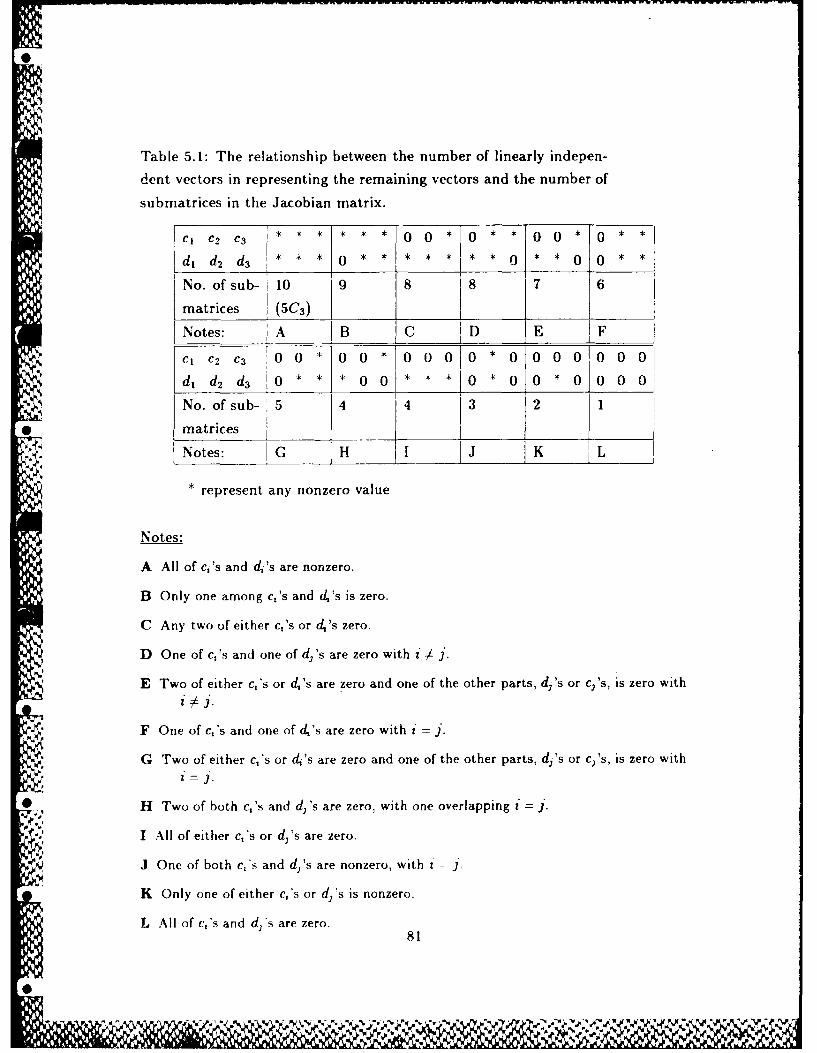
Table 5.1: The relationship between the number of linearly indepen-
dent vectors in representing the remaining vectors and the number of
submatrices in the Jacobian matrix.
CI C2 C3 * *** * 0 0 * 10 **-0 0 * 0**
d, d2 d3 ~ ~ *0**** * *0 ~ 0 0
INo. of sub- 10 98 8 7 6
Lmatrices (5C 3) ]___ ___I___ ______
Notes: A B__ C DIE F
No. of sub- 5 4 4 3 2 1
* ~~~matrices _ _ __ __ _
~Notes: G H_ __ _ K IL*represent any nonzero value
Notes:
A All of c,'s and d.,'s are nonzero.
B Only one among C,'s and d's is zero.
C Any two of either c,'s or d's zero.
D One of c,'s and one of d3's are zero with iI
E Two of either c,'s or d 's are zero and one of the other parts, d,'s or c 's, is zero with
- ~ F One of c,'s and one of d's are zero with Z'j
G Two of either c,'s or d 's are zero and one of the other parts, d3 's or c3 s, is zero with
H Two of both c1 s 'and d1 's are zero, with one overlappingZj
I All of either c, 's or d, 's are zero.
J One of both c,'s and d3 's are nonzero, with 1'-
K Only one of either c,'s or d.,'s is nonzero.
L All of c,*s and d,'s are zero. 8
%8
0%
Chapter 6
Relationship and Comparisonwith other Measures
6.1 Introduction
In this chapter, we test the new performance measure developed in the previous
chapter in order to see if it indeed helps achieve the desire performance. Also we
will examine if it has the ability of avoiding repeatability problem and problems
due to switching of the kinds of solutions.
To this end, first, we investigate the qualitative relationships of the new mea-
sure with two major performance measures introduced in Section 1.1.3: the ma-
nipulability measure and the condition number. We will also focus on the afore-
mentioned property of preventing the switching of aspects. Then, we will try
to confirm, through numerical simulations for three different manipulating situa-
tions, the points so far derived.
82
8011 z i
6.2 Relationship with Other measures
In this section, we investigate the relationship between the proposed measure and
each of the two measures: first the manipulability measure and then the condition
number.
6.2.1 the relationship to the manipulability measure
From the fact that both represent the distance from singularity, we intuitively
see that the new measure and the manipulability measure are somewhat related
to each other. However, what is more precise relationship between the two? The
* following theorem answers the question:
Theorem 3 For any matrix, J E gR"" n , with m < n,
P
det(JJT) = Z A, 2
t=1
where A 8', i = 1,2,..,p, with p = nCm, are again minors of rank m of the
matriz J.
The proof for the theorem is in Appendix 4. Since the manipulability measure,
H1, is defined as
H, = det(JJT)
it is expressed in terms of minors as follows:
H, = A (6.1)
* whereas the new measure expressed in (5.4) is again,
iH = IPAil"
Comparing the two measures, we note the following differences:
83
1. Geometrically, the manipulability measure may be interpreted as the Eu-
clidean norm of the vector representing the present state in the Al - A 2 -
... -AP coordinates system, or as the distance from the origin to the
present state in that coordinate system. The new measure, on the other
hand, represents the radius of sphere whose volume is equal to that of the
hyper-hexahedron made from the Ai, i = 1, 2,. , p coordinates in the same
coordinate system.
2. As mentioned in Section 5.5, the new measure cannot have a large value
if the value of each A, is uneven; whereas the other can have still a large
value only if some of dominant minors have large values. The manipula-
bility measure can have, in the extreme, some zero minors, as long as the
workspace rank is preserved.
Hence the new measure tends to give more balanced minors than the ma-
nipulability measure, not to mention prevents minors from being zero, thus
directly controlling over switching of aspects; whereas the manipulability
measure does not have an immediate effect on switching of aspects.
3. Note that the manipulability can be also expressed as(Yoshikawa,1985)
H, m~H 1 =1 0k a
* where 0h is the k - th singular value.
This expression shows that the measure has exactly the same form as the
new measure in that it is a product; the difference is that the manipulabil-
ity measure is the product of the singular values representing workspace,
whereas the new measure the product of minors representing the joint space.
This difference implies, in a sense, that the former concentrates on pre-
serving the workspace rank while the latter on degrees of freedom of joint
84
Millj W,
space. Since keeping maximum degrees of freedom of joint space automat-
ically preserves the workspace rank, the latter has the more sufficient yet
strict requirements.
To illustrate the second difference, let us consider the same redundant manip-
ulator in Chapter 4, which is to locate the end effector at a certain x - y position.
At the end effector location, there exist infinite numbers of configurations or sets
of joint values that enable the position, each determining a distinct Jacobian
matrix and thus a distinct set of minors.
These sets of minors accordingly determine a curve in the Al - A2 - A3 coor-
dinate system, as shown in Figure 6.1. Applying the proposed method for inverse
kinematics, when the end effector is located at x = 0.2m y = Om, we can obtain
Lwo sets of joint values that maximizes the two measures. Then their correspond-
ing sets of minors are plotted in the same curve in Figure 6.1. From the resulting
minor values plotted in the figure, one may confirm the predicted tendency: the
new performance measure gives somewhat more balanced minor values than the
manipulability measure. This tendency was also confirmed, although different in
degrees depending on the locations within the workspace: the more noticeable as
the tip moves toward the outer or inner workspace limits.
6.2.2 Relationship with the condition number
The relationship with the condition number, however, is not so clear as that with
the manipulability measure, because of the difficulty in deriving such a pair of
simple expressions as (5.4) and (6.1). As well known, the condition number H 2 is
defined as
H2 - (6.2)
where ar,,, and a,,. are minimum and maximum values of singular values, respec-
tively. As pointed out in the above subsection, since the singular values represent
85
4
qUNEMM N MO
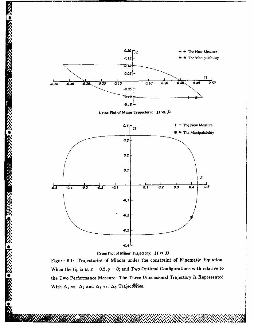
0.20 -12 + + The New Measure
0.15- The Manipulability
0.05-
0.50 .40 -0.8 -0.20 -0.10 0.10 0.20 0. 0. 0.50
Cross Plot of Minor Trajectory: J1 vs. J2
0.4 - + + The New Measure13
*t *I The Manipulability
o.11
I I I t I I l
-0.5 -0.4 -0.3 -0.2 -0.1 0.1 0.2 0.3 0.4 0.5
-0.1 -
0.3-
• 0.4-
Cross Plot of Minor Trajectory: J1 vs. J3
Figure 6.1: Trajectories of Minors under the constraint of Kinematic Equation,
When the tip is at z = 0,2, y = 0; and Two Optimal Configurations with relative to
the Two Performance Measure: The Three Dimensional Trajectory Is Represented
With A, vs. A2 and A1 vs. A3 TrajectAies.
" ' 0" I """
~%
Q2
the workspace rank, this measure, too, concentrates its concern on preserving the
workspace rank. More specifically, minimizing the condition number, in effect,
results in maximizing am,. Since nonzero value of , guarantees the workspace
rank, the measure after all tries to preserve the workspace rank. And as long
as it is preserved, it does not concern about what happens within the redundant
degrees of freedom.
6.3 Comparison of Performance measures
In this section, the new measure is quantitatively compared with the two other
measures. To this end, some numerical experiments are tried for the case of a
three degrees of freedom planar manipulator as in Chapter 4.
The points we try to examine through the experiments are as follows:
1. whether the new measure, if used for the kinematic control, helps achieve
the desired performance, that is to overcome singularity;
2. whether the measure contributes to preserve the aspect, the kind of joint
configurations, and how preserving the aspect relates to the repeatability
problem;
3. what other effects the transition of aspects brings about.
5To examine the first point, the ability to overcome singularity, simulations for the
following two cases are tried: when the manipulator has a nearly singular config-
uration; and when the end effector touches the base. To examine the second and
third points, on the other hand, the end effector is made to radially reciprocate
between the base and outer limits of the workspace.
For the kinematic control in the experiments, the two equivalent methods, the
proposed method or the resolved motion method, were alternately used depending
87
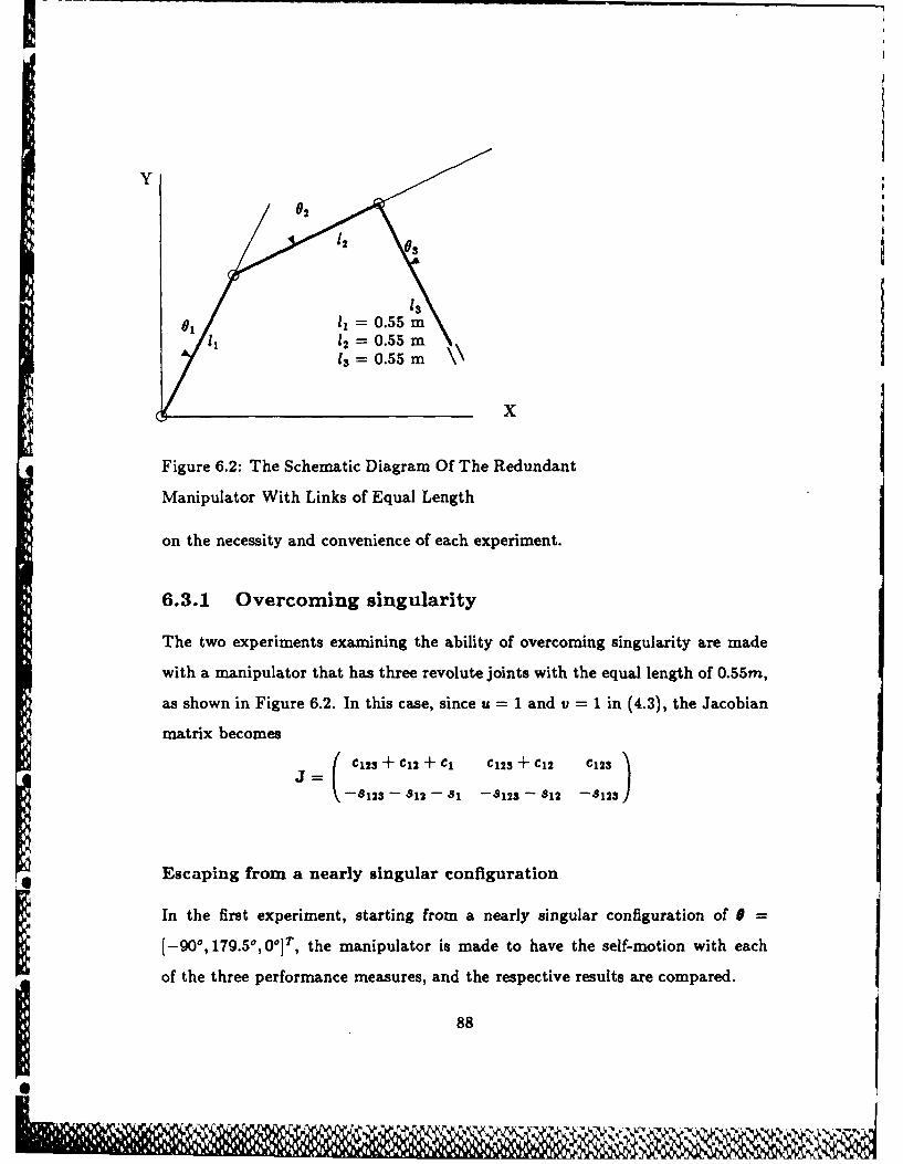
IY
02 1
013
, X
Figure 6.2: The Schematic Diagram Of The Redundant
Manipulator With Links of Equal Length
on the necessity and convenience of each experiment.
6.3.1 Overcoming singularity
The two experiments examining the ability of overcoming singularity are made
with a manipulator that has three revolute joints with the equal length of 0.55m,
as shown in Figure 6.2. In this case, since u = 1 and v = 1 in (4.3), the Jacobian
matrix becomes
( C123 + C12 + C1 C123 + C12 C123
-8123 - 812 - 81 -S123 - $12 -8123)
Escaping from a nearly singular configuration
In the first experiment, starting from a nearly singular configuration of 0 =
[-90, 179.50, 0 .1T, the manipulator is made to have the self-motion with each
of the three performance measures, and the respective results are compared.
88
Since the successive change of configurations - as time goes on - is to be
examined, the resolved motion method in (3.6), which appears the more suitable
for this purpose between the two kinematic control methods, is used with a = 10.
Of the measures, by the way, in order to avoid a large value of null space term,
the condition number is not directly minimized; instead, its inverse is maximized.
That is because the condition number has a large value at the initial state, result-
ing in a large value of h - it is proportional to the condition number - which,
in turn, causes a very large value of null space term.
89
0I
Si
s89
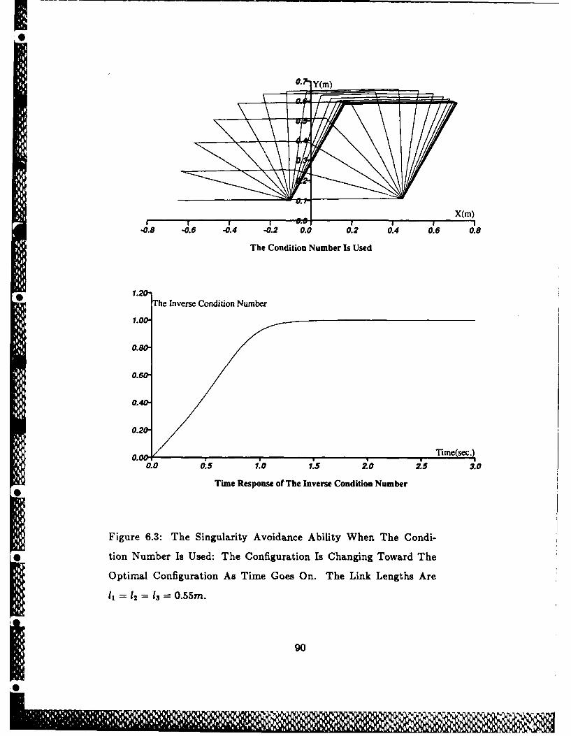
-08 -0.6 -0.4 -0.2 0.0 0.2 0.4 0.6 0.8
The Condition Number Is Used
1.20The Inverse Condition Number
1.00
0.80
0.60
0.40
0.20
0. D Time(sec.)0005101.5 2.0 2.5 3.0
Time Response or The Inverse Condition Number
Figure 6.3: The Singularity Avoidance Ability When The Condi-
* tion Number Is Used: The Configuration Is Changing Toward The
Optimal Configuration As Time Goes On. The Link Lengths Are
11 = 12 =13 0-O55M-
90
NMI
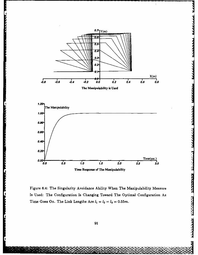
0.- Y(m)
~~~0.3. tJ'm
0.2" 7
&e X(M
__ _ __ _ __ _ __ _ __ _ _X(m)
-0.8 -0.6 -0.4 -0.2 0.0 0.2 0.4 0.6 0.8
The Manipulability is Used
1.20mThe Manipulability
1.00.
0.80-
0.60m
0.4
0.20"
0.1 nTime(sec.)
.00.5 1.0 1.5 2.0 is .0
Time Response of The Manipulability
Figure 6.4: The Singularity Avoidance Ability When The Manipulability Measure
Is Used: The Configuration Is Changing Toward The Optimal Configuration As
Time Goes On. The Link Lengths Are 11 = 12 = 13 = 0.55m.
91
4'NI
IIThe result of the experiment is given in Figures 6.3, 6.4, 6.5, where the change
9' of configurations and the time response of each measure are shown. From this
result, it is clearly demonstrated that each measure, if included in the null spaceI
term, makes the manipulator get out of the singular configuration, driving joint
values toward the state where the measure has the maximum value for the tip
location. The effect of including the performance measures becomes even more
obvious, if the self-motion without the measures is considered, when no self-motionI
happens at all because the r.h.s of (3.6) is zero. The speed of convergence for the
condition number case is noticeably slower than those of the two other measures,
both of which are almost the same.
At the steady state, whereas the condition number has a considerably different
one, the new measure and the manipulability measure have optimal configurations
that look surprisingly similar. Yet a close inspection shows that they are slightly
different. The reason for these similar configurations is as follows. The optimal
condition, Zh = 0, for each measure is in general quite different from one another.
Even for the manipulator in Figure 6.2 with such a particularly symmetric geom-
etry, joint solutions for each measure are different. However, the above optimal
condition for each measure turns out to be satisfied only at locations (x, y) of end
effector satisfying x2 + y2 = 12, with a particular joint values Of 02 = 03 = 900 or
02 = 83= -90*. Here I is the value of equal length of the three links of givenI
When passing the base
9 I]
Whereas the previous experiment examines the self-escaping ability, the present
one examines the behavior of the manipulator when the tip touches the base,
forming a closed kinematic chain - a triangle. This case is of interest because
LM '-
oviu l w the self-motion isa i t ssilenexce rd bo rotion
hapes tal bcus ter~~so (.6 s er.Th sed f ovegec 92 h
codto ubrcs sntcal lwe hntoeo h w te esrs
of the triangle with respect to the base, as long as the tip stays at that location.
This intuition can be easily confirmed if the projection matrix, I - J+J, in the
homogeneous solution term of (3.6), is symbolically derived. To be more specific,
when the tip is located at the base, the Jacobian matrix in (3.2) is modified as
the following symbolic form:
J = ( 2 3 (6.3)
0 j22 j23)
from which the projection matrix can be derived as,(10 0I-J+J= 0 0 (6.4)
0 0 0 0
Clearly, through the projection matrix, only 01 is affected by the gradient of
performance measures, h, resulting in a rigid body rotation of the triangle with
respect to the base, without making any other changes in the configuration.
Then, is it impossible for the manipulator to get into and out of the configura-
tion? In other words, can we obtain the inverse kinematic solution that resolves
the motion when the tip is passing the base? The answer for the question is that,
although the homogeneous term becomes ineffective with the tip at the base, it
is still possible for the manipulator to get into and out of the point. The reason
for the answer may be analyzed as follows:
9 When the tip approaching the base, the homogeneous solution term, al-
though diminishing, still exists, continuing the effort to achieve the optimal
configuration, until the very point of the base.
9 When the tip getting out of the base, on the other hand, now that the
projection matrix is given as in (6.4), the homogeneous term does not con-
tribute to overcoming the closed chain configuration. Yet, since the rank is
93
still preserved, the pseudoinverse J+ is available, which can be derived from
(3.4) as(0 0'
J = j23 -js (6.5)
-j22 12
Since, in this matrix, the second and the third row vectors are linearly
independent, we may have a differential tip displacement in any direction
we like in the workspace.
* Then, once the tip is apart from the base - no matter how small the
distance may be - the homogeneous term immediately begins to restore
* its effectiveness.
To sum up, at the base, where the particular solution term is still well defined,
this term drives the tip out of it, while the homogeneous term is momentarily in-
effective; at the remaining region in the workspace, on the other hand, both terms
are effective. Furthermore, between the two regions, the respective transitions of
the two terms are smooth without discontinuity.
One may suspects that the overcoming ability could have come from the inez-
act tip location - the tip can be slightly off the base - due to the linearization
characteristics of (3.6). On the other hand, inexact Jacobian matrix may have
made it possible for the tip to get out of the base, which, with the exact Jacobian
matrix, might be impossible. But these are not the cases, because both the Jaco-
bian matrix in (6.3) and the pseudoinverse in (6.5) are exact expressions defined
at an exact point, the base. Rather, the ability comes from intrinsic back-up
* function of kinematic redundancy.
The aforementioned analysis is well confirmed in the following experiment.
In the experiment, the tip is made to move along the straight line starting from
x - [0. 2 , O]T to [- 0 .2 , 0]T, passing the base, [0, O]T, with units in meters. Together
94
0
1101,
with the tip motion, the three measures are included in the inverse kinematic
method proposed in Chapter 2, which was proved to give the exact equilibrium
solution, thus excluding the effect of inaccuracy in both the tip location and the
Jacobian matrix.
From the result shown in Figures 6.6, we see that with the three measures the
manipulator had no difficulty to treat the point. We may conclude that the use
of redundant manipulator seals the hole in the workspace at the origin, where,
without the kinematic redundancy, singularity is unavoidable.
In the Figure, one may note the smoothness of motion when the new measure is
used, as compared to motions with the other measures: When the other measures
are used, the motions approaching the base from x = [0.2, 0]T are rather jerky -
see the abrupt changes in 01. The reason for the smoothness is not very clear right
now; but we can guess that keeping minors to be balanced prevents the abrupt
changes in the joint angles.
6.3.2 Preserving the aspect and its effect to the repeata-
bility problem
In the following experiment, we examine whether the manipulator, with the new
performance measure, can preserve the aspect indeed, by comparing to the cases
with other measures. The manipulator to be used for the purpose is the same one
0 -as used in the previous chapter: the three degrees of freedom planar manipulator
with revolute joints of 11 = 0.6, 12 = 0.85, and I = 0.2 with units in meters.
In the experiment, the tip is made to reciprocate radially between the base and
* the outer limit, where the manipulator fully extends. Here, the tip motion is so
made, not because the radial motion itself is of primary concern, but because it is
a way of scanning the workspace to examine the ability to preserve the aspect. To
be more specific, a series of configurations corresponding to the tip reciprocating
95
NEV
in one radial direction represent, owing to rotational symmetry, those in all the
other directions, thus covering the whole workspace. Of course, the rotational
symmetry lies in the fact that the new performance measure, together with the
other measures, depends on 82 and e3 only, and is independent of e1 - hence,
one optimal configuration for a fixed tip location is symmetrical to another for
the other tip location of the same distance from the base.
Of the two kinematic control methods, the proposed method, being the more
convenient one for obtaining the equilibrium states, is mainly used together with
the three measures. When applying the method, to solve the successive joint con-
figurations as the tip reciprocates, the present joint values are used as the initial
* conditions for the next tip location. The very first joint configurations corre-
sponding to the starting point of the tip, by the way, are determined by obtaining
the global minimum. To do this, we first find out, for comparison, all the local
minima by providing with every possible initial condition for solving the system
of nonlinear equations, (2.11). These initial conditions, in turn, may be deter-
mined by finely tessellating the joint space, that is, the domains of joint variables,
01, 02, 03. In parallel to this, all the local maxima at each tip location are obtained
with the proposed method, in order to cross-examine if the successive generations
of joint values are indeed correct. In addition to the joint configurations, cor-
responding minor values are obtained to examine the correlation between joint
configurations and minor values.
Tn Figures 6.7, 6.9, 6.11, the optimal joint configurations based on each of the
performance measures and the value of each measure are plotted.
Corresponding minor values are plotted in Figures 6.8, 6.10, 6.12.
As shown in the figures, each performance measure has two distinct sets of
configurations that, depending on the tip location, alternately give the global op-
timum. Hence, each of the two sets of configurations has its own corresponding
S
96
1111 FI J - 1 r 1r,1 .11
performance measure curve: the one, consisting of mostly the ladder-shaped con-
figurations, corresponds to the curve with a solid line; and the other, consisting
of mostly 'N'-shaped configurations, to the curve with a broken line. For conve-
nience, let us denote the former configurations A, and the latter configurations
B.
Besides, note that the mirror-image sets of Configurations A and B with re-
spect to the x-axis, although having the same values of the corresponding measure,
are not included in the figures, for brevity. Of course, there are still additional sets
of configurations that, corresponding to local maxima instead of global maxima,
are not shown in the figures either.
What do we find from the resulting configurations? Let us examine the con-
figurations generated by each performance measure one after another.
The Manipulability Measure
Figure 6.7 shows the two configurations and corresponding values of performance
measure, when the manipulability measure is used. In the figure, depending on the
tip location, each of the two configurations alternately assumes larger performance
measure value than the other. In the region between z = 1.1m and z = 1.6m,
however, the two configurations become identical, having the same performance
measure values. Then what happens with the two configurations, when the tip Is
coming out of this region of the identical configuration? To answer this question,
we need more careful observations as follows.
In Configurations A, the initial configuration is preserved within almost the
whole workspace except for the region between the base and x = 0.1m. That is,
except for this region, the initial shape does not change, regardless of wherever
the tip location may be, and to whatever direction - toward or outward from
the base - the tip may move.
97
')6 jjl 111) 11 I
In Configuration B, on the other hand, where the tip starts from near the base,
the initial configuration is preserved only if the tip is located within a certain dis-
tance from the base, about 1 m; outside the location, the configurations shift or
merge into Configuration A. And once merged, configurations corresponding to
subsequent tip motions stay within Configuration A, never returning to Configu-
ration B.
Here, we observe that the manipulator has switched the aspect or the kind
of joint solutions. Moreover the configuration, once switched from one aspect
to another, does not return to the initial configuration: the expected repeatabil-
ity problem. Then, what happened to the minors when this switching of aspect
occurred? Did they change their sign indeed, passing through zero values? Fig-
ure 6.8 clearly shows that is the case: the tip location where merging happens is
the place where one of the minors changes its sign.
The Condition Number
In the case of the condition number, the situation is even more complicated.
In this case, Configurations A consists of successive joint configurations, where
the tip starts from near outer limit of the workspace toward the base, whereas
Configuration B represents the movements in the opposite direction from the
base. Differently from the manipulability case, in both Configurations A and B,
the initial configurations are merged into the other. Furthermore, the locations
where mergings occur are different: about z = 0.7m for Configuration A; and
x = 1.3m for Configuration B. And within z = 0.7m, or outer than z = 1.3m, the
two configurations are identical, giving the same measure curve.
Hence, the repeatability problem occurs, between x = 0.7m, and x = 1.3m,
when the tip reverses its direction after experiencing a merging. Again, the mi-
nor curve in Figure 6.10 shows that, when the switchings occur, signs of minors
98
11 Id 1
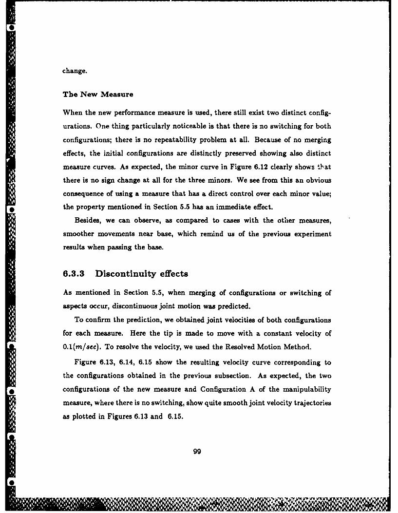
change.
The New Measure
When the new performance measure is used, there still exist two distinct config-
urations. One thing particularly noticeable is that there is no switching for both
configurations; there is no repeatability problem at all. Because of no merging
effects, the initial configurations are distinctly preserved showing also distinct
measure curves. As expected, the minor curve in Figure 6.12 clearly shows t!at
there is no sign change at all for the three minors. We see from this an obvious
consequence of using a measure that has a direct control over each minor value;
the property mentioned in Section 5.5 has an immediate effect.
Besides, we can observe, as compared to cases with the other measures,
smoother movements near base, which remind us of the previous experiment
results when passing the base.
6.3.3 Discontinuity effects
As mentioned in Section 5.5, when merging of configurations or switching of
aspects occur, discontinuous joint motion was predicted.
To confirm the prediction, we obtained joint velocities of both configurations
for each measure. Here the tip is made to move with a constant velocity of
0.1(m/aec). To resolve the velocity, we used the Resolved Motion Method.
Figure 6.13, 6.14, 6.15 show the resulting velocity curve corresponding to
the configurations obtained in the previous subsection. As expected, the two
*configurations of the new measure and Configuration A of the manipulability
measure, where there is no switching, show quite smooth joint velocity trajectories
as plotted in Figures 6.13 and 6.15.
99
2zWVM MEN
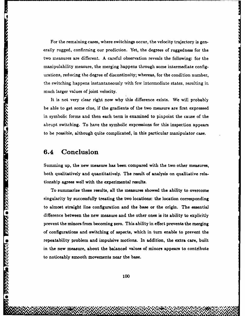
For the remaining cases, where switchings occur, the velocity trajectory is gen-
erally rugged, confirming our prediction. Yet, the degrees of ruggedness for the
two measures are different. A careful observation reveals the following: for the
manipulability measure, the merging happens through some intermediate config-
urations, reducing the degree of discontinuity; whereas, for the condition number,
the switching happens instantaneously with few intermcdiate states, resulting ir1
much larger values of joint velocity.
It is not very clear right now why this difference exists. We will probably
be able to get some clue, if the gradients of the two measure are first expressed
in symbolic forms and then each term is examined to pinpoint the cause of the
abrupt switching. To have the symbolic expressions for this inspection appears
to be possible, although quite complicated, in this particular manipulator case.
6.4 Conclusion
Summing up, the new measure has been compared with the two other measures,
both qualitatively and quantitatively. The result of analysis on qualitative rela-
tionship agrees well with the experimental results.
To summarize these results, all the measures showed the ability to overcome
singularity by successfully treating the two locations: the location corresponding
to almost straight line configuration and the base or the origin. The essential
difference between the new measure and the other ones is its ability to explicitly
prevent the minors from becoming zero. This ability in effect prevents the merging
of configurations and switching of aspects, which in turn enable to prevent the
repeatability problem and impulsive motions. In addition, the extra care, built
in the new measure, about the balanced values of minors appears to contribute
to noticeably smooth movements near the base.
100
i0 ...
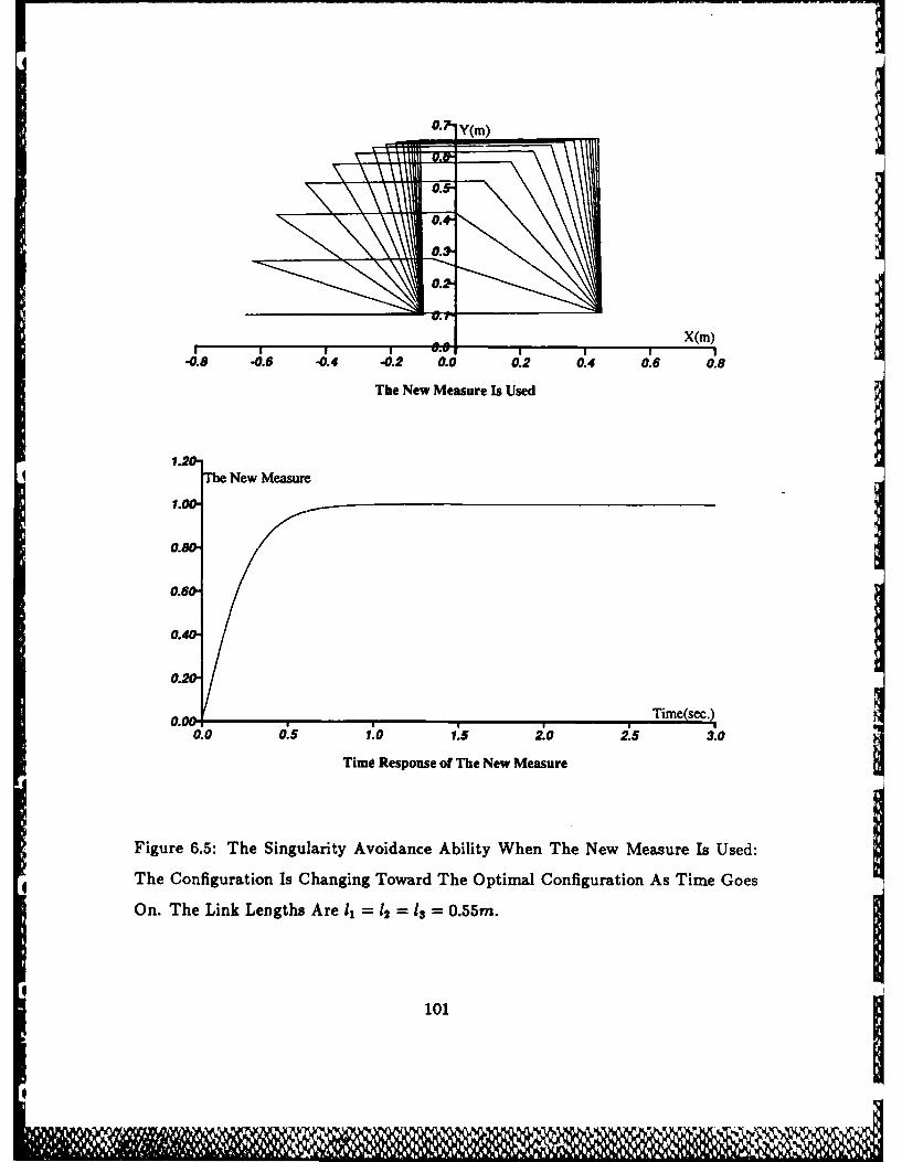
0.7 Y(m)
0.5
0.3
1.22
0.+
0.6.
1.0.
TiERsos lThe New Measure
Fiur .5:TeSnuait viac bliyWe h e MaueIsd
4 heCnfguaio I hagigToar heOpialCofguato A Tm Ge
0.0
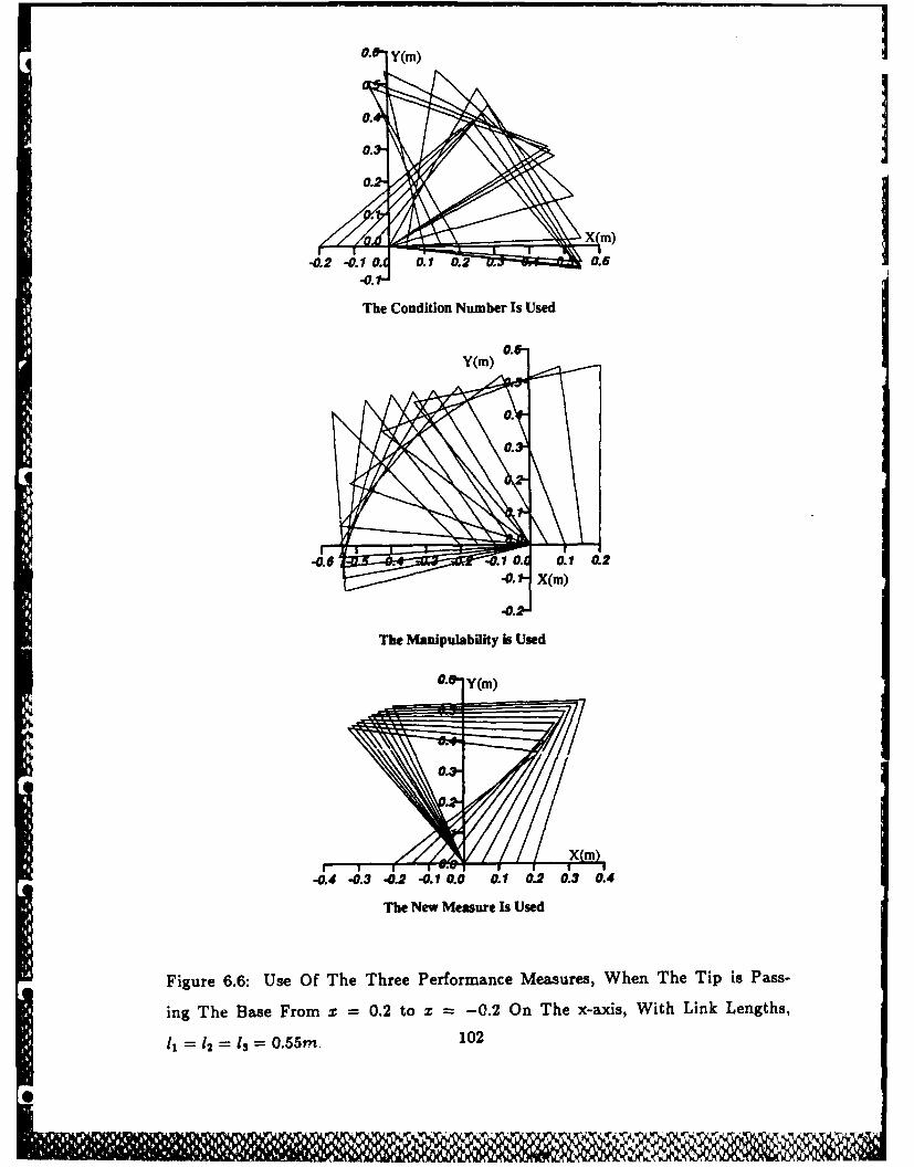
|I.Y(M)
J 0.
Io. mI
-0.2 -0.10.1 0.1 0.2 0.6-0.1-4
The Condition Number Is Used
-0.6 0 0.1 0.2
-0.- mm
2 -~0."
~The Manipulability is Used
-0.4 -0.3 -0.2 -0.1 0.0 0.1 0.2 0.3 0.4The New Measure Is Used
Figure 6.6: Use Of The Three Performance Measures, When The Tip is Pass-
ing The Base From z = 0.2 to z -0.2 On The x-axis, With Link Lengths,
11 =1 2 = 1s= 0.55m. 102
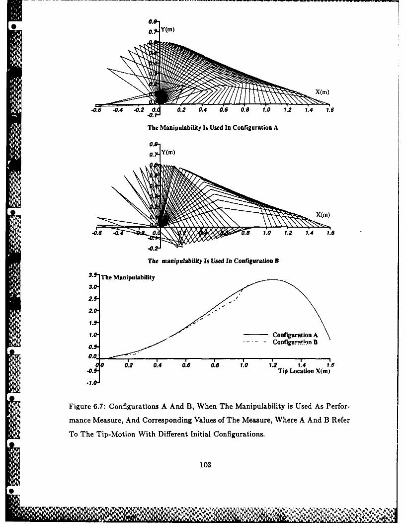
o.76 Y(M)
-0.6 -0.4 -0.2 0. 0.2 0.4 0.6 0.8 1.0 1.2 1.4 1.6
The Manipulability Is Used In Configuration A
3.0
2. 0
1.0
1.T mt Configuration A
0. - Configur',;.n B0.0 - --
I II I I !01.0 1.2 1 6
-o.F Tip Location X(m)
-1.0
Figure 6.7: Configurations A And B, When The Manipulability is Used As Perfor-
mance Measure, And Corresponding Values of The Measure, Where A And B Refer
To The Tip-Motion With Different Initial Configurations.
0103
-0..,,
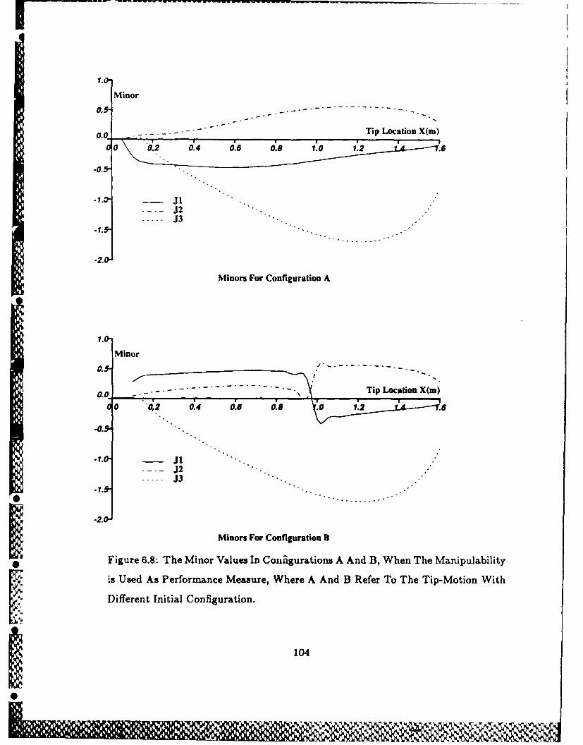
0
O.CL Tip Location X(m)
0 00 0.4 0.6 0.d 10o.
J12
-1.0
Minor
00 '0,2 0.4 0.6 0.8 .0 1.
J12................ J3
-20
Minors For Configuration B
* Figure 6.8: The Minor Values In Coriigurations A And B, When The Manipulability
is Used As Performance Measure, Where A And B Refer To The Tip-Motion WithI Different Initial Configuration.
104
0w
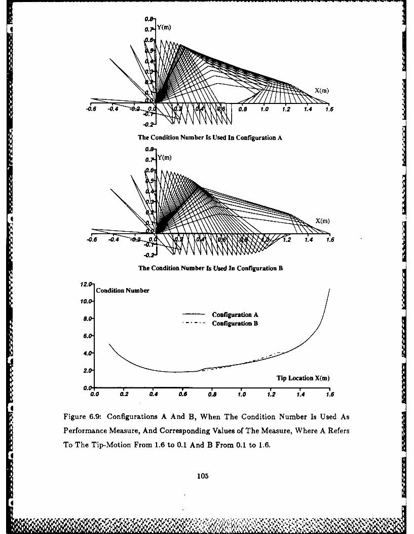
[! O.6 Y(m)i
0.8 i40.i 1.0 1.2 1.4 1.6
The Condition Number Is Used In Configuration A
4(M jThe Condition Number Is Used In Configuration B
12.0Condition Number
10.0"
8.I Configuration A-.--- Configuration B
6.0
4.0
Tip Location X(m)
0.0 S 080.0 0.2 .4 0.6 1. 1.4 1.6
Figure 6.9: Configurations A And B, When The Condition Number Is Used As
Performance Measure, And Corresponding Values of The Measure, Where A Refers
To The Tip-Motion From 1.6 to 0.1 And B From 0.1 to 1.6.
0"105 g
4.0
2.0-.~ S
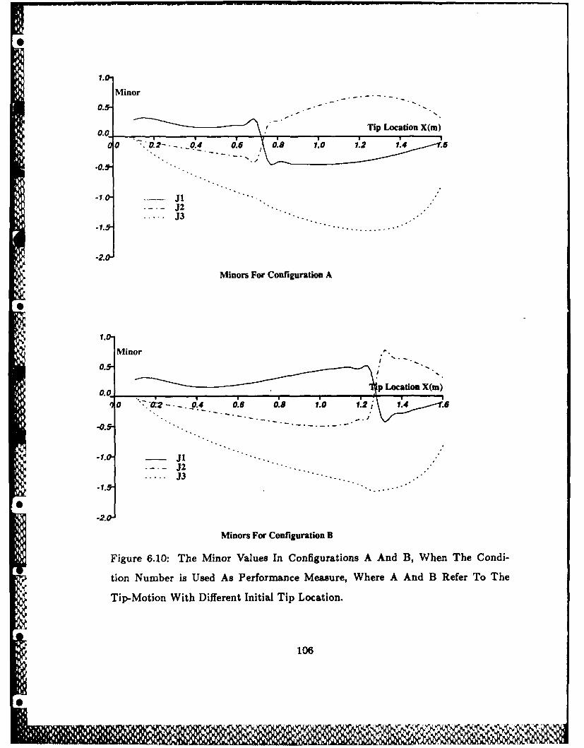
1.0
0.-Minor
00 -. 0.2- - -0 f.4 0.6 0.0 1.0 1.2 1.4 .6
J2.. . J3
= Minors For Configuration A
1.0
Minor0.5
0 i.:-...p4 0.6 0.8 1.0 1.2, 14 .
...................J3
Minors For Configuration B
Figure 6.10: The Minor Values In Configurations A And B, When The Condi-
tion Number is Used As Performance Measure, Where A And B Refer To The
Tip-Motion With Different Initial Tip Location.
106
; j
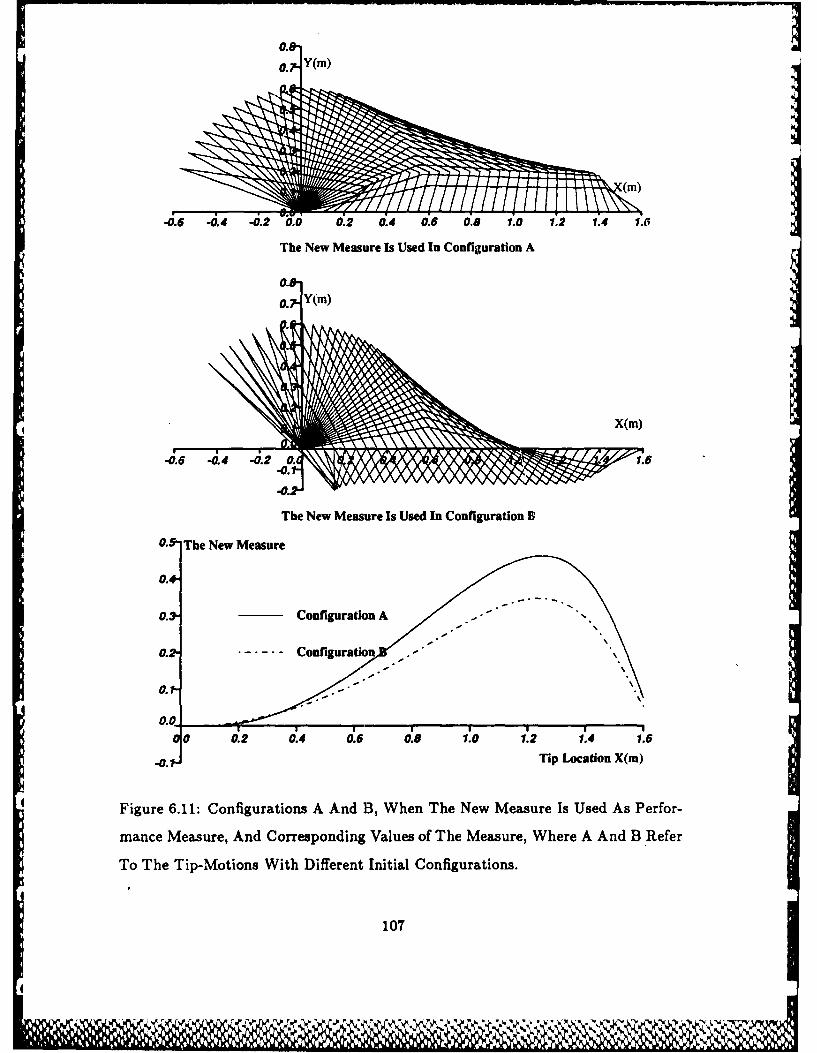
~~0.2,. Y(m) '
-0.6 -0.4 -0.2 0.0 0.2 0.4 0.6 0.8 1.0 1.2 1.4 1.6
The New Measure Is Used In Configuration A
k
0.7 Y(m)
X(m)
r(
-0.6 -0.4 -0.2 0. 1.6j -0.1J ~~-0.2-
The New Measure Is Used In Configuration B
0.5- The New Measure
0.+
0.3- Configuration A
0.2 - ----- Configuration -
0.r.
0.0r0 02 0.4 0.6 0.8 1.0 1.2 1.4 1.6
-0. Tip Location X(m)
Figure 6.11: Configurations A And B, When The New Measure Is Used As Perfor-
mance Measure, And Corresponding Values of The Measure, Where A And B Refer
To The Tip-Motions With Different Initial Configurations.
107
4
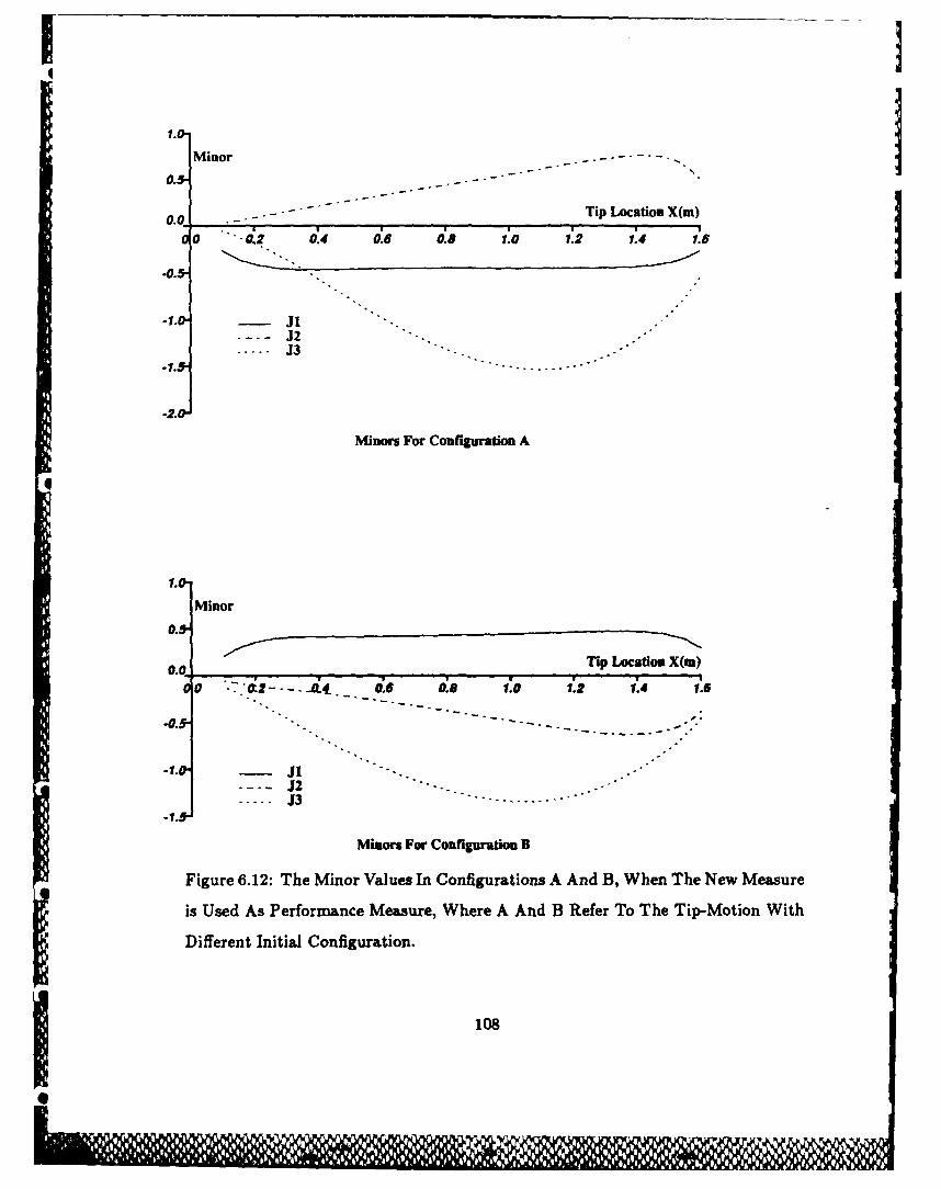
Minor
0.0. - - Tip Location X~u)
00 0,2 0W4 0.6 0.8 1.0 1.2 1'4 1.6I
J2... J3
-1. . . . . . . . .
-2.O
Minors For Configuration A
1.0
Minor
0.5
00.0 r. U.ip Location X(mn)0 i 01- 06 0i8 1.0 1.2 1.4 1.6
J2
Minors For Configuration B
Figure 6.12: The Minor Values In Configurations A And B, When The New Measure
is Used As Performance Measure, Where A And B Refer To The Tip-Motion With
Different Initial Configuration.
108% ljrj I
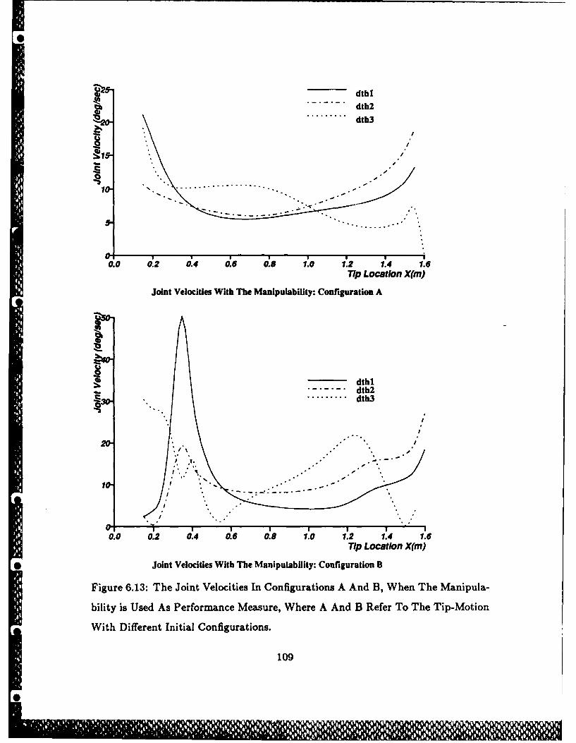
dthldth2dth3
S/A
*'" . -.. . -'- - "10-~ ............
00.0 0.2 0.4 0.6 0.8 1.0 1.2 1.4 1.6
Tip Location X(m)
Joint Velocities With The Manipulability: Configuration A
qb
~dthl. . . dth23 "........ dth3
., '"
0.0 0.2 0.4 0.6 0.8 1.0 1.2 1.4 1.6Tip Location X(m)
*Joint Velocities With The Manipulability: Configuration B
Figure 6.13: The Joint Velocities In Configurations A And B, When The Manipula-
bility is Used As Performance Measure, Where A And B Refer To The Tip-Motion
With Different Initial Configurations.
109
0i
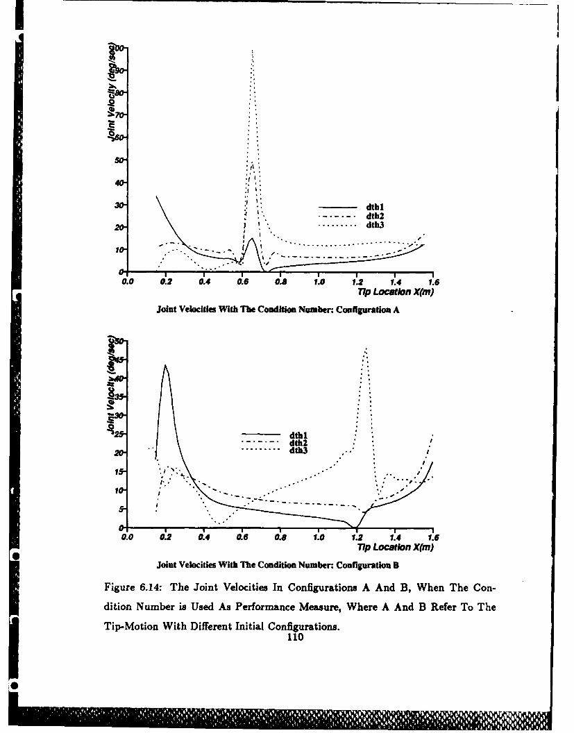
4-
30- dthl.- - --- -- dth2
20- .. ..... dth3
0-0.0 0.2 0.4 0.6 0.8 1 .0 1.2 1.4 1 .6
Tip Location X(m)
Joint Velocities With The Condition Number: Configuration A
2& dtb3
010.0 0.2 0.4 0.6 0.8 1.0 1.2 1.4 1.6
Tip Location X(m)
Joint Velocities With The Condition Number: Configuration B
Figure 6.14: The Joint Velocities In Configurations A And B, When The Con-
dition Number is Used As Performance Measure, Where A And B Refer To The
Tip-Motion With Different Initial Configurations.110
0j
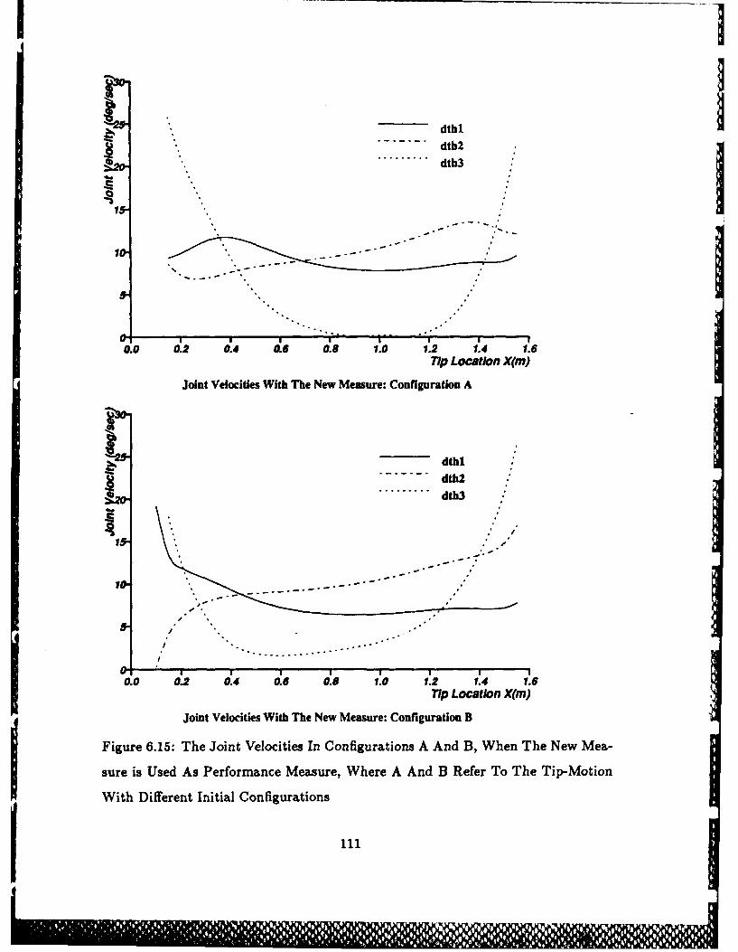
it -.- -. dthl
dth2.... .... dth3
10
ILI
I III
0.0 0.2 0.4 0.6 0.8 1.0 1.2 1.4 1.6Tip Location X(m)
Joint Velocities With The New Measure: Configuration A
dthldth2
. . . . . . . . . . . .. . . . . . . . . . . . . . . . . . . d th 3
10.1
1-
0.0 0.2 0.4 0.6 0.8 1.0 1.2 1.4 1.6Tip Location X(m)
Joint Velocities With The New Measure: Configuration B
Figure 6.15: The Joint Velocities In Configurations A And B, When The New Mea-
sure is Used As Performance Measure, Where A And B Refer To The Tip-Motion
With Different Initial Configurations
il1111111
Chapter 7
Conclusion
In this thesis, some important aspects of kinematic control problems have been
investigated. These aspects may be categorized into two main themes: One is the
formulation of a new general the inverse kinematic method for redundant arms.
The other is the development of a new dexterity measure.
Finding a concise yet general formulation is important for the exploitation of
kinematic redundancy. Furthermore, the fact that the equation is formulated at
the inverse kinematic level is significant because it has the advantage of directly
mapping from workspace to joint space. The relationship between the new formu-
lation and existing ones such as the Resolved Motion Method has been analyzed.
Among various desired performances, the dexterous configurations are not
yet well understood. By explicitly defining the dexterity as the distance from
the kinematic singularity, one can have a good springboard for approaching this
rather ambiguous concept. This distance concept in fact helps illuminate the
less known fact that for a particular degree of redundancy there are different
degrees of distance from singularity. This finding in turn immediately leads to a
performance measure for controlling this distance. An analysis of the relationship
of the new measure with similar measures confirms that our approach is sound
112
1 1%
and useful.
In the light of these two themes, each chapter is reviewed as follows. Chapter
2 covers the derivation of the proposed formula, the interpretation of its charac-
teristics, and estimation of computational efficiency. In addition, the new formula
was there compared to the existing formula and it is shown that the new formula
is a general, yet concrete expression of the others.
In Chapter 3, we qualitatively compared this formula with the Resolved Mo-
tion Method. From the comparison we analytically showed that the proposed
formula is in fact a direct mapping counterpart of the other method. That is,
the proposed formula was proved to provide directly the equilibrium states at
which the joint variables in the other method eventually arrive if the end effec-
tor is made to stop at a fixed location. In addition, Resolved Motion Method
was shown to lead to non-repeatable behavior. We also proposed a differential
relationship, equivalent to the other method, yet based on the proposed formula,
which is shown to be slightly more efficient.
In Chapter 4, numerical experiments were made to verify the theoretical and
qualitative results so far obtained. Also the numerical efficiency of the new
method was compared with the Resolved Motion Method. The theoretical re-
sults confirmed through the simulations were as the following:
" the Resolved Motion Method is a linearized equation approximated at the
equilibrium points that are exactly determined by the proposed formula;
" the repeatability problem persists in the Resolved Motion Method in tran-
sient period as well as at the steady states.
In addition, a practical way to use the proposed formula in a real time control sit-
uation was considered in conjunction with an efficient joint interpolation method
devised by Taylor. Tho comparison of efficiency with the other ,ptlnd %hv'.'
that the proposed formula is more efficient when higher accuracy is required.
113
In Chapter 5, we have defined the concept of dexterity as a distance from
singularity. Then we reviewed the concept of singularity and redundancy for
further investigation of the distance concept. We have illustrated that there are
different degrees of distance from singularity in the same degree of redundancy,
showing that the conventional concept of redundancy is not sufficient to describe
this distance. The new distance concept we derived was the number of nonzero
minors as well as the magnitude of each minor. On the base- of the new concept,
a new performance measure was derived.
In Chapter 6, we have related the new performance measure with the manip-
ulability measure and the condition number. Having investigated the qualitative
relationship, we pointed out that the other measures do not have the ability to
explicitly prevent minors from becoming zero. Through another series of nu-
merical experiments, the effect of this ability was clearly confirmed. Whereas
the two other measures without this ability showed repeatability problem and
discontinuous motions, the new measure consistently overcame these problems.
114
1 '61 1111 'l, 1P 1 1 I II ,I K II I I 11 1
I
Appendices
Appendix 1: Taylor's Bounded Deviation Algo-
rithm
In this Appendix, we briefly introduce Taylor's bounded deviation algorithm. The
algorithm consists of two parts: one part is to generate appropriate numbers of
via points and joint angles that guarantee given deviation from Cartesian path;
the other part interpolates the joint angles to obtain better resolution. The first
part is summarized in the following scheme.
Taylor's Bounded Deviation Joint Paths
1. Compute the joint values 00 and 01, corresponding to xo and xi, respectively.
2. * Compute the joint space midpoint, 0,, = (01 + 01)/2, and use it to
compute f,, = f(0,).
* Also, compute the workspace midpoint, x, = (x0 + x 1)/2
3. Compute the deviation between fm and x,,, 6 = Ixm - fIl
4. If 6 < 6 "' , we are done. Otherwise, compute the joint value 0, f -'(x,);
and apply steps 2-4 recursively, for the two segments (x0 - xm) and
(Xm, , x,).
I115
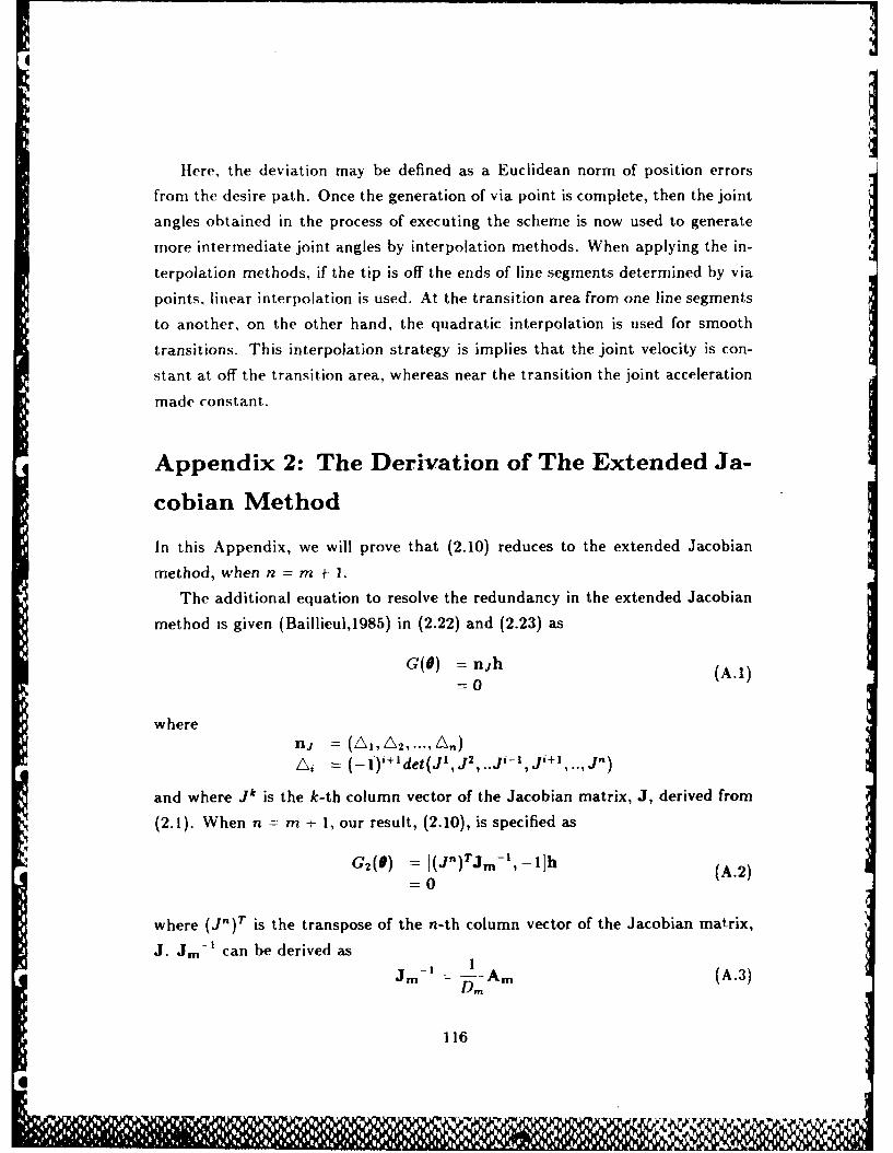
Here, the deviation may be defined as a Euclidean norm of position errors
from the desire path. Once the generation of via point is complete, then the joint
angles obtained in the process of executing the scheme is now used to generate
more intermediate joint angles by interpolation methods. When applying the in-
terpolation methods, if the tip is off the ends of line segments determined by via
points, linear interpolation is used. At the transition area from one line segments
to another, on the other hand, the quadratic interpolation is used for smooth
transitions. This interpolation strategy is implies that the joint velocity is con-
stant at off the transition area, whereas near the transition the joint acceleration
made constant.
Appendix 2: The Derivation of The Extended Ja-
cobian Method
In this Appendix, we will prove that (2.10) reduces to the extended Jacobian
method, when n = m + 1.
The additional equation to resolve the redundancy in the extended Jacobian
method is given (Baillieul,1985) in (2.22) and (2.23) as
G(8) njh (A.1)=0
wherenj =L i/k = (- l)i+1det(J', j2,.J i-I, Ji+1 .. ,J n.
and where jk is the k-th column vector of the Jacobian matrix, J, derived from
(2.1). When n = m + 1, our result, (2.10), is specified as
G2 (0) = (jn)rJm-l, -1]h (A.2)II =0
where (jn)T is the transpose of the n-th column vector of the Jacobian matrix,
J. JmI can be derived as
Jm-- Am (A.3)DmA
116
U 1 z
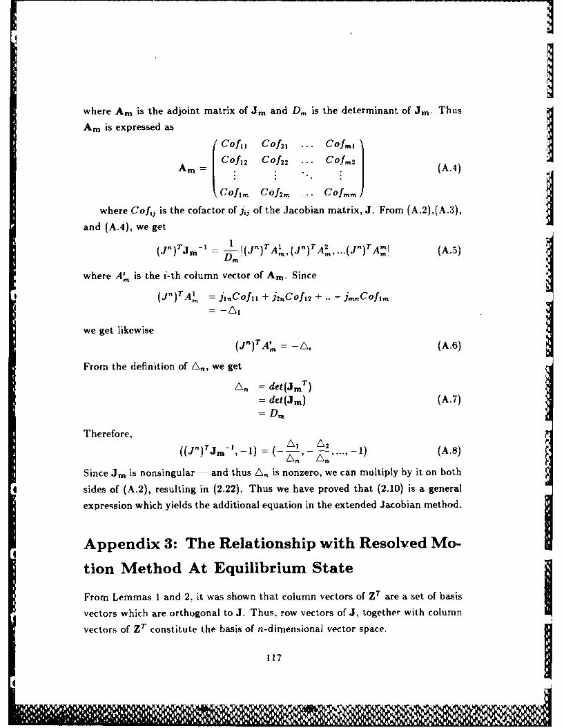
k-
where Am is the adjoint matrix of Jm and Dm is the determinant of Jm- Thus
Am is expressed as
Cofl Cof21 ... Cofm\
Am Cof12 Cof 22 ... COf,,,2 A4)
COfirn COf 2 ,. C.. Cfm
where Cofi, is the cofactor of j,, of the Jacobian matrix, J. From (A.2),(A.3),
and (A.4), we get
(dn)Tj._ , 1 (jn)T A', (jn)T A 2,...(jn)T Aml (A.5)- M DM -
where A, is the i-th column vector of Am. Since
TJ A' =I- jiCofll + j 2,1Cofl2 + .. + janCOfim
1"-A
we get likewise_ (j,)Ta A' -A (A.6)
From the definition of A,, we get
'!' = det(jm T )= det(Jm) (A.7)
Therefore,((jfl)Tjm-,_) - A, A2 1) (A.8)
Since Jm is nonsingular -- and thus /A is nonzero, we can multiply by it on both
sides of (A.2), resulting in (2.22). Thus we have proved that (2.10) is a general
expression which yields the additional equation in the extended Jacobian method.
Appendix 3: The Relationship with Resolved Mo-
tion Method At Equilibrium State
From Lemmas I and 2, it was shown that column vectors of ZT are a set of basis
vectors which are orthogonal to J. Thus, row vectors of J, together with column
vectors of ZT constitute the basis of n-dimensional vector space.
117
11 1 1 , 1 '14I
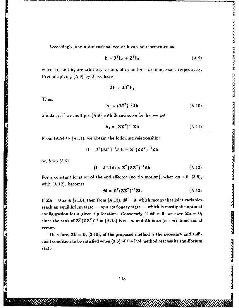
J6
I
Accordingly, any n-dimensional vector h can be represented as
h = jTh, + ZTh 2 (A.9)
where h, and h2 are arbitrary vectors of m and n - m dimensions, respectively.
Premultiplying (A.9) by J, we have
Thus,
h, = (JJT)-'Jh (A.10)
Similarly, if we multiply (A.9) with Z and solve for h 2 , we get Ih2 = (ZZT)-IZh (A.11)
From (A.9) to (A.11), we obtain the following relationship:
(I JT(jjT) -'J)h = ZT(ZZT)-Zh
or, from (3.5),
(I - J+J)h z ZT(ZZT)-'Zh (A.12)
For a constant location of the end effector (no tip motion), when dx =O, (3.6),
with (A.12). becomes
d = ZT(ZZT) -Zh (A.13)
If Zh = 0 as in (2.10), then from (A.13), dO = 0, which means that joint variables
reach an equilibrium state - or a stationary state - which is mostly the optimal
configuration for a given tip location. Conversely, if df = 0, we have Zh = 0;
since the rank of ZT(ZZT) - l in (A.13) is n - m and Zh is an (n - m)-dimensional
vector.
Therefore, Zh = 0, (2.10), of the proposed method is the necessary and suffi-
cient.condition to be satisfied when (3.6) nf0- RM method reaches its equilibrium
Appendix 4: Proof of Theorem 3
In this appendix, we make a proof of Theorem 3. The Jacobian matrix is expressed
as the following:
11z I11
Then En=, j,2 ... nE
JJT( k= Iimkjl iiJm2
In general, the determinant of an m x m matrix A is explicitly given as
where a1, is the element of A at i'-th row and j -th column, ur (a, 0,., v) with
distinct integers, a,,3, - -,v =1,2, - - -,m, PO is the permutation matrix, and
I ,means the sum is taken all m! permutations of or. Hence, the determinant of
jjT is
det (jj 2 ) F(Z jlIA~k)(YZ j2kJ,3k) .. (II jickju) det(Per)0 k=1 k=I k=1
Expanding this, we have
U ki, ,.,=l
Here, note that terms that have non-distinct k,'s disappears. For instance, if
k2 k 1, then 1iGJ1/ 1 ,mvmdisappears when a 1 and ;3 2.
Thus, in Equation A.15, summation is applied only to the terms with distinct
k,'s. Note also that the number, p, of different sets of distinct k,'s is
p =nCm.
Rearranging Equation A.15, we have
de., ( jjT) J (Zj0ikj2k," j .mkdet (Pa)) (j*QkJo3k, ~J . kJ vk)ki, ,k,,=i 0
I 19
Here summation k .1 may be divided into
n P
E = :k * k,,, -l t=1 (7,
where a, =(k, k2,. ,) is i-th set of p different sets consisting of Fr distinct
k,'s. Therefore Equation A.15 becomes
33k,, I C 2 J
If we denote a part of Equation A. 16 as
.N C ,J , ,/ e PU
Comparing this with Equation A.14 shows that A, is the determinant of the
transpose of the subrnatrix made of k,'s cLolumn vectors as
A, =det (~jkj jk2 ... jk. IT)
where P, is the k,-th column vector of the Jacobian matrix. Once a set of k,'s
is chosen, the absolute value of A, is fixed; only its sign changes as k,'s make
permutations. If we set the absolute value as jAj, Equation A.16 becomes
Pdet (jj T ) -zZ~ Ai(Z Jk~J2k!, * ,J mk,,, det (PUM)
The facts that the determinant of a matrix is equal to that of transpose of the
*matrix and that jjT is positive definite imply that
p
det (jjT) F, AZ2 .
Q.EI. D.
120
I n6
Appendix 5: Proof for Derivation of Joint Veloc-
ity from the Optimizing Equation
Since Z spans the null space of j, we have
ZJT = 0 (A.17)
Hence, multiplying both sides of (A.17) by (jjT)-1, we have
ZJT(JJT)- I =0 (A.18)
Using the relationship, J+ = ZJT(jjT) -1, we derive from (A.18)
0ZJ + = 0
Meanwhile the definition of the pseudoinverse matrix is again,
J J+ =Im
where Im is the identity matrix of rank m. Combining the above two equations
results in a composite equation,
where the composite matrix is denoted as
JE J (A.20)
Multiplying both sides of (A.19) by JE1 results in
QE. D.
121
0
I
References
Albala,H, and Angeles,J., 1979, " Numerical Solution to the Input-Output Dis-placement Equation of General 7R Spatial Mechanism," Proc. 5th World Cong.Theory Mech. Mechanism, Montreal, pp. 1008-1011.
Angeles, J., 1985, "On the numerical solution of the inverse kinematic problem,"Int. J. Robotics Research, 4 no. 2, pp. 21-37.
Baillieul, J., Hollerbach, J.M., and Brockett, R., 1984, "Programming and con-trol of kinematically redundant manipulators," Proc. 23rd IEEE Conference onDecision and Control, Las Vegas, Nevada, December 12-14, pp. 768-774.
Baillieul, J., 1985, "Kinematic programming alternatives for redundant manipu-lators," Proc. IEEE Conf. Robotics and Automation, St. Louis, Mar. 25-28,pp. 722-728.
Baillieul, J., 1986, "Avoiding obstacles and resolving kinematic redundancy,"Proc. IEEE Int. Conf. Robotics and Automation, San Francisco, April 7-10,pp. 1698-1704.
Benati, M., Morasso, P., and Tagliasco, V., 1982, "The inverse kinematic problemfor anthropomorphic manipulator arms," ASME J. Dynamic Systems, Meas.,Control, 104, pp. 110-113.
Benhabib, B., Fenton, R.G., and Goldenberg, A.A., 1984, "Point-to-point controlof seven degrees of freedom robots for assembly operations," Proc. 3rd CanadianCAD/CAM and Robotics Conf., Toronto, pp. 10/1-10/7.
Benhabib, B., Goldenberg, A.A., and Fenton, R.G., 1985, -A solution to the
122
II
inverse kinematics of redundant manipulators," Proc. American Control Conf.,Boston, June 19-21, pp. 368-374.
Ben-lsrael,A. and Greville,T., 1980, Generalized Inverses: Theory and Applica-tions, New York, Robert E. Krieger Publishing Co..
Borrei, P., and Liegeois, A., 1986, "A study of multiple manipulator inverse kine-matic solutions with applications to trajectory planning and workspace determi-nation," Proc. IEEE Int. Conf. Robotics and Automation, San Francisco, April7-10, pp. 1180-1185.
Chang, P.H., 1986, "A closed-form solution for the control of manipulators withkinematic redundancy," Proc. IEEE Int. Conf. Robotics and Automation, SanFrancisco, April 7-10, pp. 9-14.
Espiau, B., and Boulic, R., 1985, "Collision avoidance for redundant robots withproximity sensors," Preprints 3rd International Symposium of Robotics Research,Gouvieux (Chantilly), France, October 7-11, pp. 94-102.
Featherstone, R., 1983, "Position and velocity transformations between robotend-effector coordinates and joint angles," Int. J. Robotics Research, 2 no. 2, pp.35-45.
Goldenberg, A., Benhabib, B., and Fenton, R.G., 1985, "A complete generalizedsolution to the inverse kinematics of robots," IEEE J. Robotics and Automation,1, pp. 14-20.
Goldenberg, A.A., and Lawrence, D.L., 1985, "A generalized solution to the in-verse kinematics of robotic manipulators," ASME J. Dynamic Systems, Meas.,Control, 107, pp. 103-106.
Gupta, K.C., and Kazerounian, K., 1985, "Improved numerical solutions of inversekin,'natics of robots," Proc. IEEE Int. Conf. Robotics and Automation, St.Louis, March 25-28, pp. 743-748.
Hamming,R., 1973, Numerical Methods for Scientists and Engineers (2nd ed.),* New York, McGraw-Hill, Inc..
Hartenburg, R. S., and Denavit, J., 1964, Kinematic Synthesis of Linkages, NewYork, McGraw-Hill.
Hollerbach,J.,Suh,K., 1986, "Redundant Resolution of Manipulators ThroughTorque optimization," A./.Memo 882, Cambridge, January.
123
6T
Hollerbach, J.M., 1985, "Optimum kinematic design for a seven degree of freedommanipulator," Robotics Research: The Second International Symposium, editedby H. Hanafusa and H. Inoue, Cambridge, Mass., MIT Press, pp. 215-222.
Klein, C.A., 1985, "Use of redundancy in the design of robotic systems," RoboticsResearch: The Second International Symposium, edited by H. Hanafusa and H.Inoue, Cambridge, Mass., MIT Press, pp. 207-214.
Klein, C.A., and Huang, C.H., 1983, "Review of pseudoinverse control for use withkinematically redundant manipulators," IEEE Trans. Systems, Man, Cybern.,SMC-13, pp. 245-250.
Konstantinov, M.S., Markov, M.D., and Nenchev, D.N., 1981, "Kinematic controlof redundant manipulators," Proc. l1th Int. Symp. on Industrial Robots, Tokyo,Japan, October 7-9, pp. 561-568.
Liegeois, A., 1977, "Automatic supervisory control of the configuration and be-havior of multibody mechanisms," IEEE Trans. Systems, Man, Cybern., SMC-7,pp. 868-871,
Luh, J.Y.S., and Gu, Y.L., 1985, "Industrial robots with seven joints," Proc.IEEE Conf. Robotics and Automation, St. Louis, Mar. 25-28, pp. 1010-1015.
Maciejewski, A.A., and Klein, C.A., 1985, "Obstacle avoidance for kinematicallyredundant manipulators in dynamically varying environments," Int. J. RoboticsResearch, 4 no. 3, pp. 109-117.
Mathlab Group, 1983, "MACSYMA Reference Manual," Version 10, Mas-sachusetts Institute of Technology, Laboratory for Computer Science, Cam-bridge, MA..
Mor6,J., Garbow,B., and Hillstrom,K., 1980, User Guide for MINPACK-1, Ar-gonne National Laboratory.
Nakamura, Y., 1985a, Kinematical Studies on the Trajectory Control of RobotManipulators, Ph.D. Thesis, Kyoto Univ., June.
Nakamura, Y., and Hanafusa, H., 1985b, "Task priority based redundancy controlof robot manipulators," Robotics Research: The Second International Symposium,edited by H. Hanafusa and H. Inoue, Cambridge, Mass., MIT Press, pp. 155-162.
Nakamura, Y., and Hanafusa, H., 1985c, "Inverse kinematic solution with singu-larity robustness for robot manipulator control," ASME Winter Annual Meeting:
124
Robotics and Manufacturing Automation, PED- Vol. 15, Miami Beach. Nov.17-22, pp. 193-204.
Oh,S.Y., Orin,D.E., and Bach,M, 1984, "An Inverse Kinematic Solution for Kine-tratically Redundant Robot Manipulators," Journal of Robot Systems, Summer,pp. 235-249.
Orin, D.E., and Schrader, W.W., 1984, "Efficient Jacobian determinaton for robotmanipulators," Robotics Research: The First International Symposium, edited byM. Brady and R. Paul, Cambridge, Mass., MIT Press, pp. 727-734.
Paul, R.P., September, 1975, "Manipulator Path Control," Proc. Intl. Conf.Cybernetics and Society, New York, pp. 147-152.
Paul, R.P., 1979, "Manipulator Cartesian path control," IEEE Trans. Systems,~ Man, Cybernetics, SMC-9, pp. 702-711.
Paul, R.P., 1981, Robot Manipulators: Mathematics, Programming, and Control,Cambridge, Mass, MIT Press.
Paul, R. P., and Stevenson, C. N., 1983, "Kinematics of robot wrists," Int. J.Robotics Research, 2 no. 1, pp. 31-38.
Pieper, D.L., 1968, The Kinematics of Manipulators under Computer Control,Ph.D. Thesis, Stanford University, Computer Science.
Rabinowitz, P., 1970, Numerical Methods for Nonlinear Algebraic Equations, NewYork. Gordon and Breach Science Publisher, Inc..
Salisbury, J. K., and Craig, J. J., 1982, "Articulated Hands: Force Control andKinematic Issues," The International Journal Of Robotics Research, in press.
Strang, G., 1980, Linear Algebra and its applications, New York, Academic Press.
Taylor, R.H., 1979, "Planning and execution of straight-line manipulator trajec-tories," IBM Journal of Research and Development, 23, pp. 424-436.
Uchiyama, M., 1979, "Study on Dynamic Control of Artificial Arm - Part 1,"JSME, in press.
Uchiyama, M., Shimizu, K., and Hakomori, K., 1985, "Performance evaluationof manipulators using the Jacobian and its application to trajectory planning,"Robotics Research: The Second International Symposium, edited by H. Hanafusa
125
0
0
and H. Inoue, Cambridge, Mass., MIT Press, pp. 447-456.
Whitney, D.E., 1969, "Resolved motion rate control of manipulators and humanprostheses," IEEE Trans. Man-Machine Systems, MMS-10, pp. 47-53.
Whitney, D.E., 1972, "The mathematics of coordinated control of prosthetic armsand manipulators," ASME J. Dynamic Systems, Meas., Control, pp. 303-309.
Yoshikawa, T., 1984, "Analysis and Control of Robot Manipulators with Redun-dancy," Robotics Research: The First International Symposium, edited by M.Brady and R. Paul, Cambridge, Mass., MIT Press, pp. 439-446.
Yoshikawa, T., 1985a, "Manipulatability of Robotic Mechanisms," Robotics Re-search: The Second International Symposium, edited by H. Hanafusa and H.Inoue, Cambridge, Mass., MIT Press, pp. 439-446.
Yoshikawa, T., 1985b, "Analysis and Design of Articulated Robot Arms from theViewpoint of Dynamic Manipulability," Preprints 3rd International Symposiumof Robotics Research, Gouvieux(Chantilly), France, October 7-11, pp. 150-156.
0
0
i 126
0
I
List of Figures
1.1 The Schematic Diagram Of The Manipulator System ........ . . 7
3.1 The Relationship Between The Proposed Method And The Re-
solved Motion Method; The Direct Mapping And The DifferentialMapping ........................................ 44
4.1 The Schematic Diagram Of The Redundant Manipulator ...... .51
4.2 Joint trajectories obtained with the two methods: The Three Di-mensional Trajectory Is Represented With 01 vs. 02 and 01 vs. 03
Trajectories ...................................... 56
4.3 The command path and actual workspace trajectories obtainedwith the two methods ...... ......................... 57
4.4 The Achievable Accuracy Of Tip-Location With The Two MethodsWith Relative To The Iteration Numbers ................... 58
4.5 The Change of Deviation From the Desired Path, As the Via PointsChanges. Note That The Deviation Is Changing Exponentially. . . 65
6.1 Trajectories of Minors under the constraint of Kinematic Equation,When the tip is at x = 0.2, y = 0; and Two Optimal Configura-tions with relative to the Two Performance Measure: The ThreeDimensional Trajectory Is Represented With A, vs. A2 and A, vs.A 3 Trajectories .................................... 85
6.2 The Schematic Diagram Of The Redundant Manipulator WithLinks of Equal Length ...... ......................... 87
127
t11)ilil jllir ilii
•-
6.3 The Singularity Avoidance Ability When The Condition Num-ber Is Used: The Configuration Is Changing Toward The Op-timal Configuration As Time Goes On. The Link Lengths Are IIi = 12 = 13 = 0.55m. ................................ 89
6.4 The Singularity Avoidance Ability When The Manipulability Mea-sure Is Used: The Configuration Is Changing Toward The Op-timal Configuration As Time Goes On. The Link Lengths AreI = 12 = 13 = 0.55m ................................. 90
6.5 The Singularity Avoidance Ability When The New Measure IsUsed: The Configuration Is Changing Toward The Optimal Con-figuration As Time Goes On. The Link Lengths Are 11 = 12 = 13 =
0.55m .......................................... 100
6.6 Use Of The Three Performance Measures, When The Tip is PassingThe Base From x = 0.2 to x = -0.2 On The x-axis, With LinkLengths, 11 = 12 13 = 0.55M .......................... 101
6.7 Configurations A And B, When The Manipulability is Used AsPerformance Measure, And Corresponding Values of The Measure,Where A And B Refer To The Tip-Motion With Different InitialConfigurations.....................102
Co fg r to s . . . . . . . . . . . . . . . . . . . . . . . . . . . . .. 10
6.8 The Minor Values In Configurations A And B, When The Manip-ulability is Used As Performance Measure, Where A And B ReferTo The Tip-Motion With Different Initial Configuration ...... .103
6.9 Configurations A And B, When The Condition Number Is Used AsPerformance Measure, And Corresponding Values of The Measure,Where A Refers To The Tip-Motion From 1.6 to 0.1 And B From
0.1 to 1.6 ....................................... 104
6.10 The Minor Values In Configurations A And B, When The Condi-tion Number is Used As Performance Measure, Where A And BRefer To The Tip-Motion With Different Initial Tip Location. . . 105
6.11 Configurations A And B, When The New Measure Is Used AsPerformance Measure, And Corresponding Values of The Measure,Where A And B Refer To The Tip-Motions With Different InitialConfigurations ...... ............................. 106
128
6.12 The Minor Values In Configurations A And B, When The NewMeasure is Used As Performance Measure, Where A And B ReferTo The Tip-Motion With Different Initial Configuration ...... .. 107
6.13 The Joint Velocities In Configurations A And B, When The Manip-ulability is Used As Performance Measure, Where A And B ReferTo The Tip-Motion With Different Initial Configurations ..... 108
6.14 The Joint Velocities In Configurations A And B, When The Con-dition Number is Used As Performance Measure, Where A And BRefer To The Tip-Motion With Different Initial Configurations. 109
6.15 The Joint Velocities In Configurations A And B, When The NewMeasure is Used As Performance Measure, Where A And B ReferTo The Tip-Motion With Different Initial Configurations ..... .. 1100
129
0j il I
List of Tables
4.1 The comparison of accuracy and repeatability obtained with thetwo methods at the first cycle, when transient effect is visible.. . . 59
4.2 The comparison of accuracy and repeatability obtained with thetwo methods at the steady state, when the tip reciprocates a ver-tical line-segment ........ ............................ 60
4.3 The comparison of solutions: Proposed Method vs. RM Method.For RM Method, self-motion was iteratively made by setting dx=O. 61
5.1 The relationship between the number of linearly independent vec-tors in representing the remaining vectors and the number of sub-matrices in the Jacobian matrix ...... .................... 80
130