Control of Quadrocopter

V E D R A N S I K I R I C

Master of Science Thesis Stockholm, Sweden 2008

Control of Quadrocopter

V E D R A N S I K I R I C

Master’s Thesis in Computer Science (30 ECTS credits) at the School of Electrical Engineering Royal Institute of Technology year 2008 Supervisor at CSC was Henrik Christensen Examiner was Stefan Carlsson TRITA-CSC-E 2008:027 ISRN-KTH/CSC/E--08/027--SE ISSN-1653-5715 Royal Institute of Technology School of Computer Science and Communication KTH CSC SE-100 44 Stockholm, Sweden URL: www.csc.kth.se

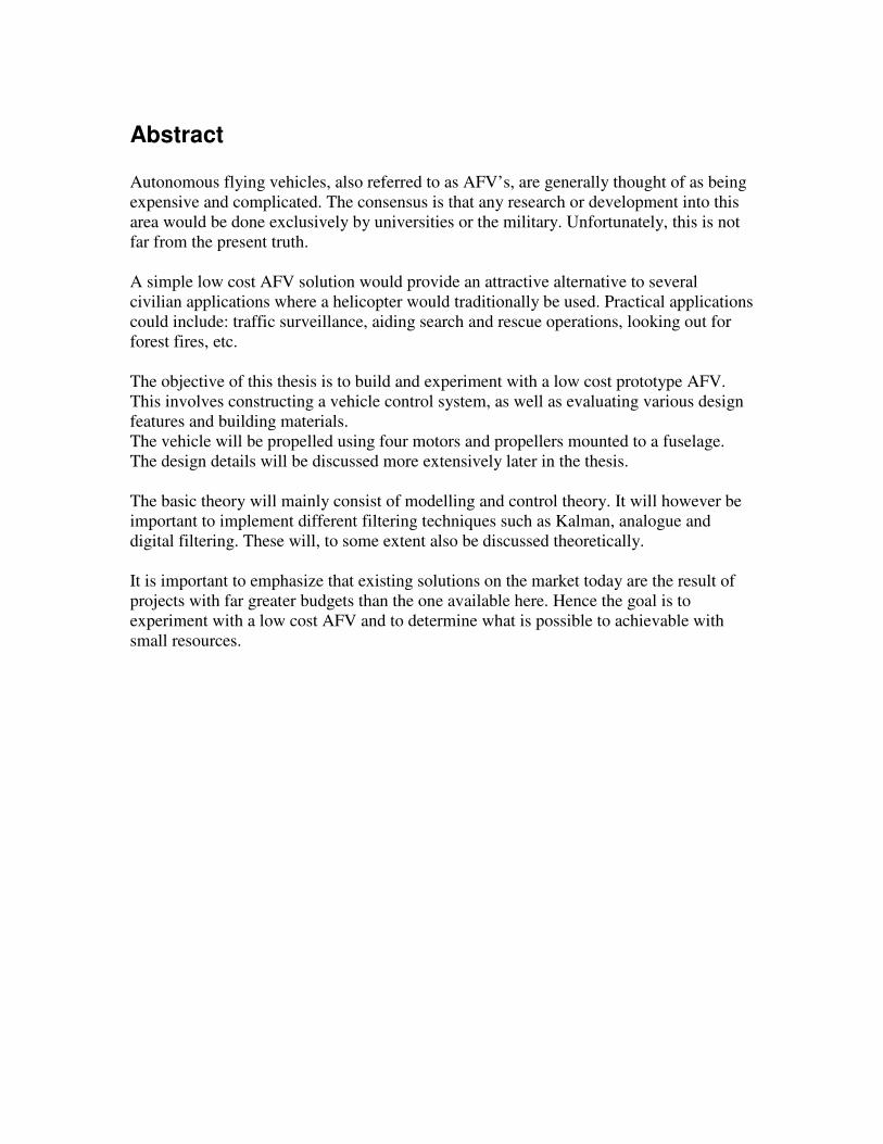
Abstract Autonomous flying vehicles, also referred to as AFV’s, are generally thought of as being expensive and complicated. The consensus is that any research or development into this area would be done exclusively by universities or the military. Unfortunately, this is not far from the present truth. A simple low cost AFV solution would provide an attractive alternative to several civilian applications where a helicopter would traditionally be used. Practical applications could include: traffic surveillance, aiding search and rescue operations, looking out for forest fires, etc. The objective of this thesis is to build and experiment with a low cost prototype AFV. This involves constructing a vehicle control system, as well as evaluating various design features and building materials. The vehicle will be propelled using four motors and propellers mounted to a fuselage. The design details will be discussed more extensively later in the thesis. The basic theory will mainly consist of modelling and control theory. It will however be important to implement different filtering techniques such as Kalman, analogue and digital filtering. These will, to some extent also be discussed theoretically. It is important to emphasize that existing solutions on the market today are the result of projects with far greater budgets than the one available here. Hence the goal is to experiment with a low cost AFV and to determine what is possible to achievable with small resources.

Styrning av quadrocopter

Sammanfattning Autonoma flygande farkoster, också kallade AFV, är generellt ansedda att vara dyra och väldigt komplexa. En följd av detta skulle vara är att majoriteten av all forskning och utveckling inom området utförs av militärindustrin eller universitet. Detta är i dagens läge tyvärr inte långt från den verklighet vi befinner oss i.

En enkel och billig AFV-lösning skulle kunna erbjuda ett attraktivt alternativ i flertalet civila applikationer där man idag använder sig av en helikopter. Exempel på sådana områden skulle kunna vara trafikövervakning, hjälpa till vid räddningsuppdrag, övervaka och hålla utkik efter skogsbränder etc. Målet med detta examensarbete är att bygga och experimentera med en lågprisvariant på en AFV. Detta i inkluderar såväl reglering och styrning av AFV’n som utvärdering av olika byggmetoder och material. AFV’n kommer att drivas med fyra stycken propellermotorer som monteras på en flygkropp. Närmare detaljer kring utformningen av AFV’n kommer att tas upp längre fram i rapporten. De teoretiska delarna i rapporten kommer framför allt att beröra områden som modellering och reglerteori. Det kommer emellertid också vara aktuellt att behandla olika filtreringstekniker så som Kalman-filter, analoga och digitala filter. Dessa kommer att diskuteras teoretiskt till viss utsträckning. Det är viktigt att påpeka att existerande AFV-lösningar som finns på marknaden idag är resultat av projekt med väldigt mycket större budgetar än vad som finns tillgängligt i detta examensarbete. Följaktligen är målet med detta examensarbete att experimentera med en lågpris-AFV och fastställa vad som är möjligt att åstadkomma med små ekonomiska medel.

Table of contents 1 Introduction...................................................................................................................... 1

1.1 Report outline............................................................................................................ 1 1.2 List of all pictures, graphs and tables used in the report........................................... 3 1.3 Background ............................................................................................................... 5 1.4 Objectives ................................................................................................................. 6 1.5 Limitations ................................................................................................................ 6 1.6 Related work ............................................................................................................. 6

1.6.1 Predator .............................................................................................................. 7 1.6.2 Draganfly ........................................................................................................... 8

2 Selecting hardware........................................................................................................... 9 2.1 Motors and propellers ............................................................................................... 9 2.2 Speed controllers..................................................................................................... 11 2.3 Eyebot ..................................................................................................................... 11 2.4 Gyrocube................................................................................................................. 12 2.5 Anti alias filter ........................................................................................................ 13 2.6 Power supply and cabling ....................................................................................... 13 2.7 Chapter summary.................................................................................................... 14

3 Problem analysis ............................................................................................................ 15 3.1 Modelling the system.............................................................................................. 15

3.1.1 Modelling the motors and propellers ............................................................... 16 3.1.2 Physical modelling........................................................................................... 19

3.1.2.1 Altitude model .......................................................................................... 19 3.1.2.2 Angle model.............................................................................................. 21

3.2 System control ........................................................................................................ 24 3.2.1 Altitude control ................................................................................................ 24 3.2.2 Pitch and bank control ..................................................................................... 28 3.2.3 Yaw control...................................................................................................... 31

3.3 Chapter summary.................................................................................................... 31 4 Hardware design ............................................................................................................ 32

4.1 Materials ................................................................................................................. 32 4.2 Building the model.................................................................................................. 33

4.2.1 Prototype A ...................................................................................................... 33 4.2.2 Prototype B ...................................................................................................... 35

4.3 Control unit ............................................................................................................. 35 4.3.1 Anti alias filter ................................................................................................. 37 4.3.2 Power supply.................................................................................................... 38

4.4 Chapter summary.................................................................................................... 38 5 Software design.............................................................................................................. 39

5.1 Overall software design .......................................................................................... 39 5.2 Sensor bias .............................................................................................................. 41 5.3 Kalman estimator .................................................................................................... 42 5.4 PID design............................................................................................................... 44 5.5 Chapter summary.................................................................................................... 45

6 Implemented system ...................................................................................................... 46 6.1 Software .................................................................................................................. 46 6.2 Hardware................................................................................................................. 47 6.3 Chapter summary.................................................................................................... 49

7 Testing............................................................................................................................ 50 7.1 Hardware testing ..................................................................................................... 50

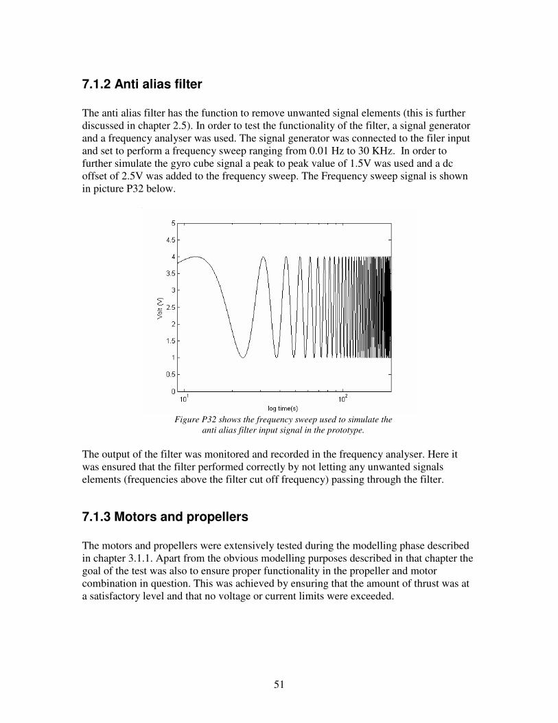
7.1.1 Power supply.................................................................................................... 50 7.1.2 Anti alias filter ................................................................................................. 51 7.1.3 Motors and propellers ...................................................................................... 51 7.1.4 Gyro cube......................................................................................................... 52

7.2 Software testing ...................................................................................................... 52 7.2.1 Pitch and bank control testing.......................................................................... 52 7.2.2 Yaw control testing .......................................................................................... 53 7.2.3 Altitude control testing .................................................................................... 54

7.3 Chapter summary.................................................................................................... 54 8 Conclusions and summary ............................................................................................. 55

8.1 Issues for future development................................................................................. 57 References......................................................................................................................... 58 Appendices........................................................................................................................ 60

Appendix A Motor data ....................................................................................... 60 Appendix B Speed controller data ....................................................................... 62 Appendix C Eyebot data ...................................................................................... 63 Appendix D Gyrocube data ................................................................................. 65 Appendix E Linear approximation calculations in MatLab................................. 67 Appendix F Modelling calculations with MatLab ............................................... 68 Appendix G Filtering algorithm in C code .......................................................... 69 Appendix H Bias removal in C code ................................................................... 70 Appendix I Kalman estimator in C code............................................................. 72 Appendix J Anti alias filter calculations.............................................................. 75 Appendix K PID in C code ................................................................................... 77

Acknowledgments

Fist of all I would like to thank my supervisor, Professor Henrik Christensen for giving me the opportunity to work on this exciting master thesis. Without him taking the time to guide me through the various problems that were encountered, the thesis would not have been as instructive and interesting. I would like to thank Silvio Sikiric for showing great patience with reading my report and correcting my English spelling and grammar, also for giving me a lesson in RC airplane construction, providing me with tools and helpful building tips. I also have to say thank you to the employees at Söders RC hobby for providing me with critical information regarding RC equipment. Their help really made my work easier. Finally I must thank my dear family for putting up with me during the thesis. The seemingly endless periods of building, soldering and programming never left them tired of me or my work. Thank you!

1

1 Introduction

Chapter 1 will give a general introduction to autonomous flying vehicles and to the thesis in general. The introduction will present an outline of the report and a list of all pictures, graphs and tables used in the thesis. This will be followed by the thesis background and objectives. The chapter is ended with a short declaration of the thesis limitations and related work.

1.1 Report outline

The chapters are presented below and give a description of the outline of the thesis. The outline also gives an insight to the methodology of the thesis. Chapter 1 is an introductory chapter. Chapter 2, this chapter is intended to give insight into some of the considerations that had to be made during the initial hardware selection process. The hardware components are presented and in some cases compared with different alternatives. Chapter 3 is more theoretical and explains how the simulation of the system was conducted. The chapter is divided in to two main sections. The first section concerns the modelling of the system and the second is focusing on the control simulation. Chapter 4 describes the design of hardware components needed for the prototype. It also discusses different materials suitable for the prototype. Chapter 5 presents the software developed within the thesis. It will give an overall software solution and a detailed description regarding the different software components. This chapter will also present some theoretical discussions. Chapter 6 is a presentation of the final system. It is also a discussion regarding the various implemented system components. Chapter 7 will address the testing of the system. It will mainly consider control issues, how the testing was conducted and how results were measured. It will also to some degree address testing of the hardware designed in previous chapters. Chapter 8 will sum up the results obtained in the thesis and relate to the theory presented in previous chapters. It will also present suggestions to future developments and discussions regarding this.

2

References will clarify and give additional information regarding sources referred to in the report. Printed literature is referred to as: “Title” by “author” [x] in the report, where x is the index number used to easily identify the complete source information in the references chapter. Internet pages are referred to in a similar manner as “the internet page” “name” [wx], where x is the index of the reference. Appendices will present additional information which could be of interest to some readers but contains too much detail to include in the report.

3

1.2 List of all pictures, graphs and tables used in the report

Figure P1 Shows version B of the predator, can conduct multiple missions simultaneously due to its large internal and external payload capacity. Figure P2 is showing the draganfly X-pro. It presents a similar platform to the intended design for the model in the thesis.

Figure P3 is showing the motor chosen for the thesis. The name of the motor is GWS EPS350CS and it includes gearing with the ratio of 5.33:1. Figure P4 shows the speed controller GWS ICS-480 which was used in the thesis. The picture also shows the heat sink and connectors. Figure P5 shows the front side of the eyebot card used during the development of the flying model. Figure P6 shows the thrust produced at different servo outputs, each motor is represented with a different colour. Figure P7 shows the linear approximation, obtained after using the least square method. Figure P8 shows the step response corresponding to the final model of the motors and propellers. Figure P9 shows the principal physical characteristics of the prototype, when it is subject for the altitude control. Figure P10 shows the principal physical properties of the prototype when it is using its motors to correct the pitch or bank angle. Figure P11 shows the simplified system if the prototype is not built with the centre of gravity at the same level as the propellers. Figure P12 shows the simulink block diagram used to simulate the altitude control. Figure P13 shows a graph of the input step. It is important to ensure control robustness both in descending and ascending situations. For this reason several steps were put together to create the input Figure P14 shows the calculated motor input signal. This is a simulation of the signal which is sent to the speed controller from the eyebot card. It is often desirable to create a control which outputs a smooth motor signal. In our case the motors are equipped with smoothening capacitors to low pass filter the signal.

4

Figure P15 shows the simulated response of the prototype. Figure P16 shows the simulink block diagram used to simulate the angle control. Figure P17 shows a graph of the input step. The step of one radian may seem as a rather large step, it is however easier to use a standardised measure when assessing system performance. Figure P18 shows the calculated motor input signal. This is a simulation of the signal which is sent to the speed controller from the eyebot card. It is often desirable to create a control which outputs a smooth motor signal. In our case however the motors are equipped with smoothening capacitors to low pass filter the signal. Figure P19 shows the simulated response of the prototype. Table T1 present the results regarding control parameters of the simulated system. Figure P20 gives an overall presentation of the prototype A. Figure P21 shows a better view of the electrical component compartment. This picture also shows the polystyrene and plywood layers inside of the compartment. Figure P22shows one of the engine mounts. Figure P23 shows the control unit. It consists of all stationary hardware that is to be used during development of the prototype. Figure P24 shows the schematics of the second order Butterworth filter used as the anti alias filter. Figure P25 shows the schematics of the power supply. Figure P26 gives a graphical display of the program structure used during the design of the AFV software. Figure P27 shows how the motor signal consists of several different PID signals controlling different states. Figure P28 gives an overview of the prototype including the motors and propellers, the body and sensors. Picture P29 shows the angle of the arms, giving the prototype a centre of gravity better suiting the modelling results discussed in section 3.1.2.2. Figure P30 gives a better view of the gyro cube sensor in the middle of the prototype and the motor speed controllers at the base of each arm.

5

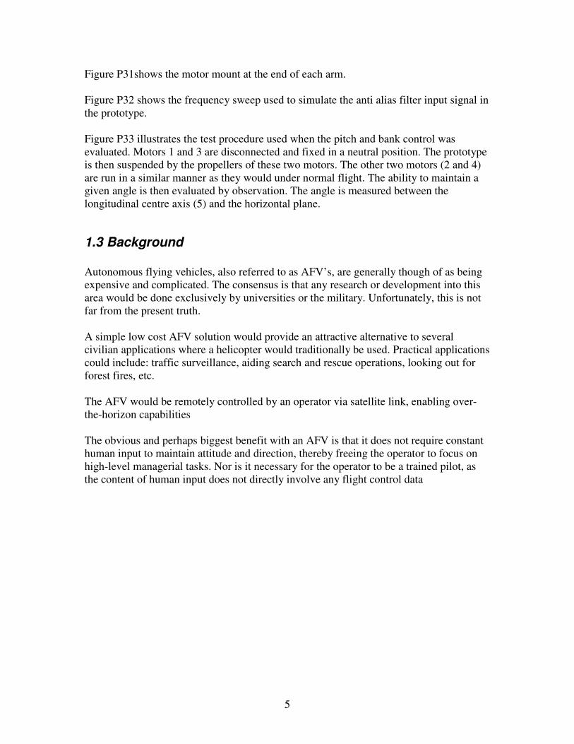
Figure P31shows the motor mount at the end of each arm. Figure P32 shows the frequency sweep used to simulate the anti alias filter input signal in the prototype. Figure P33 illustrates the test procedure used when the pitch and bank control was evaluated. Motors 1 and 3 are disconnected and fixed in a neutral position. The prototype is then suspended by the propellers of these two motors. The other two motors (2 and 4) are run in a similar manner as they would under normal flight. The ability to maintain a given angle is then evaluated by observation. The angle is measured between the longitudinal centre axis (5) and the horizontal plane.

1.3 Background

Autonomous flying vehicles, also referred to as AFV’s, are generally though of as being expensive and complicated. The consensus is that any research or development into this area would be done exclusively by universities or the military. Unfortunately, this is not far from the present truth. A simple low cost AFV solution would provide an attractive alternative to several civilian applications where a helicopter would traditionally be used. Practical applications could include: traffic surveillance, aiding search and rescue operations, looking out for forest fires, etc. The AFV would be remotely controlled by an operator via satellite link, enabling over-the-horizon capabilities The obvious and perhaps biggest benefit with an AFV is that it does not require constant human input to maintain attitude and direction, thereby freeing the operator to focus on high-level managerial tasks. Nor is it necessary for the operator to be a trained pilot, as the content of human input does not directly involve any flight control data

6

1.4 Objectives

The objective of this thesis is to build and experiment with a low cost prototype AFV. This involves constructing a vehicle control system, as well as evaluating various design features and building materials. The vehicle will be propelled using four motors and propellers mounted to a fuselage. The prototype will be approximately 60 cm in diameter and built using light materials such as balsa wood, thin pine beams or carbon fiber beams and polystyrene. The design details will be discussed more extensively later in the thesis. The desired capabilities of the prototype (AFV) is for it to be able to hold an assigned position in three dimensions using only accelerometer- and gyro sensors The basic theory will mainly consist of modelling and control theory. It will however be important to implement different filtering techniques such as Kalman, analogue and digital filtering. These will, to some extent also be discussed theoretically.

1.5 Limitations

When considering the objectives as described above, one is faced with nearly endless possibilities regarding hardware- and software design. It is important to emphasize that the existing solutions on the market today could only have been realized through far greater budgets than the one available for this thesis. Hence the goal is to experiment with a low cost AFV and to determine what is possible to achievable with small recourses. The goal is not to create a complete AFV system. It is also important to mention that the goal for the prototype is for it to be autonomous in the sense that it will be self stabilizing and able to manoeuvre to a designated position. The thesis will not address obstacle avoidance or other high level robotic behaviour, nor will it address optimization issues, but rather attempt to find one possible solution to the problem.

1.6 Related work

Many attempts have been made by people to achieve autonomy in various flying vehicles. The common denominator for all the well functioning systems is the level of complexity. These AFV’s are very complicated with many sensors and a substantial amount of computing power. This is usually analogous with high development costs leading to the fact that most implementations of AFV’s are high cost military operations. Section 1.4 will present a selection of the flying vehicles studied for this thesis. Due to the great secrecy surrounding the projects it is difficult to specify the exact capabilities of the vehicles. A brief presentation will however follow in the sub section below.

7

1.6.1 Predator

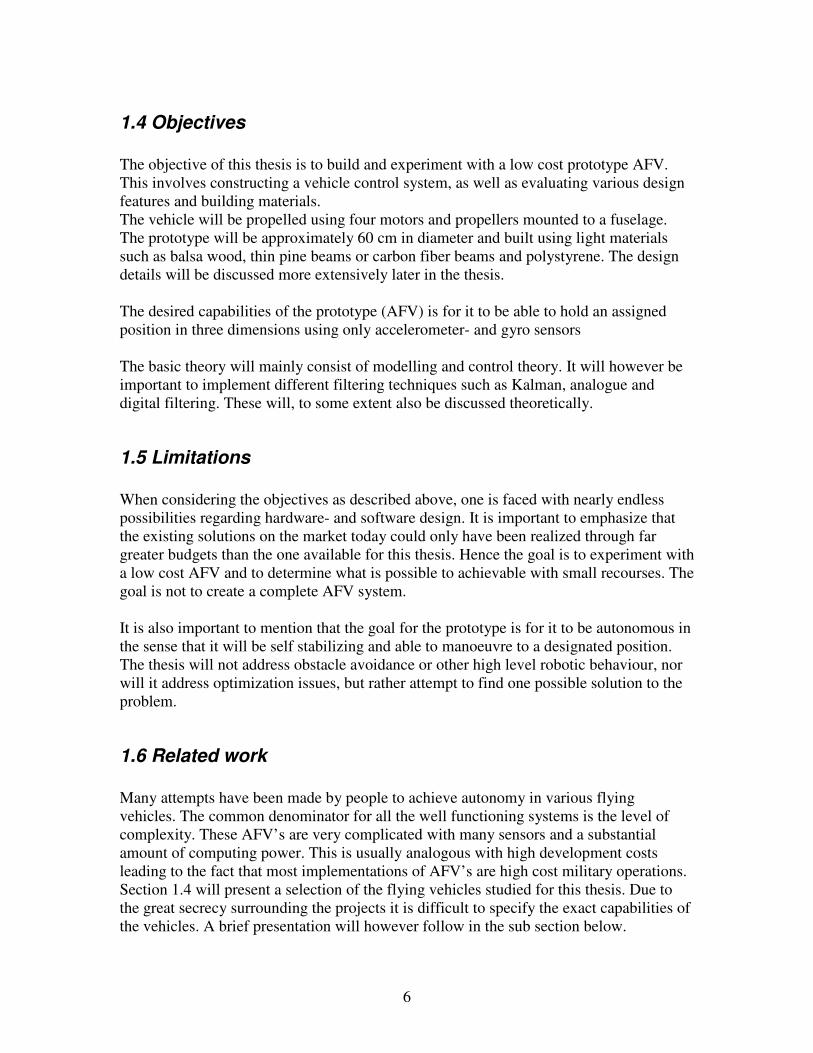
The predator is a long endurance, medium altitude unmanned aircraft system for surveillance and reconnaissance missions. It has a satellite data link to provide over-the-horizon mission capabilities. There are several different versions of the predator optimized for various situations. Predator B is shown in figure P1 below.

Figure P1 Predator B can conduct multiple missions

simultaneously due to its large internal and external

payload capacity.

Other versions can deliver surveillance imagery from synthetic aperture radar, video cameras and a forward looking infra-red (FLIR). These can be distributed in real-time both to the front line soldier and to the operational commander or worldwide in real-time via satellite communication links. More of the predator can be read of on the air force-technology internet page [W1]. A typical Predator system configuration would include four aircrafts, one ground control system and one data distribution terminal.

8

1.6.2 Draganfly

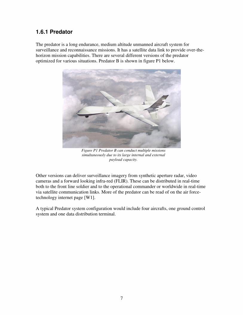
The Draganflyer X-Pro is a four rotor, radio controlled, electronically stabilized flying platform. The X-Pro is highly manoeuvrable, and has full pitch, roll, yaw, and altitude control using a conventional RC helicopter radio control transmitter. It does not qualify as an autonomous flying vehicle, since it is not capable to operate without flight control input. Even though the draganfly is more in the RC toy category it is presented here because of the basic features of the design. It is very similar to the intended design of the model in this thesis. More than so it uses MEMS gyros to help stabilizing it. The same type of sensors is going to be used in presented project. By viewing the flight demo video on the draganfly internet page [W2] it is possible to better anticipate the flight characteristics of the model that is going to be built for the project. A picture of the draganfly is shown in figure P2 below.

Figure P2 is showing the draganfly X-pro.

It presents a similar platform to the intended design for the

model in the thesis.

9

2 Selecting hardware This chapter is intended to give insight into some of the considerations that had to be made during the initial hardware selection process. Selecting the correct hardware is always critical as any poor choice of components can result in adverse effects on performance or possibly even negate basic functionality. The chapter will only address the hardware needed to solve specific problems within the confines of prototype development, thus not taking into consideration any alternative components that might be better suited for later stages of the prototype development.

2.1 Motors and propellers

The radio controlled aircraft market offers a wide selection of motors and propellers as means of propulsion. The first issue to solve when it comes to choosing a suitable motor is whether an electric motor or a combustion motor is best suited for the project. Internal combustion engines offer a good power to weight ratio and would pose a suitable alternative for a larger vehicle, intended for outdoor use. Internal combustion engines are however noisy, expensive and generate a lot of exhaust. These characteristics are considered as drawbacks in this case, as most of the development work will be conducted indoors in a test bench environment. When considering electrical motors there are two main categories.

• The brushless electrical motor. This alternative is the more exclusive one of the two, with better efficiency and longer life time. It is however much more expensive and not easily accessible with respect to control of the motor.

• The brushed electrical motor is the ordinary DC motor. It is considered to be the simpler one of the two electrical alternatives. The most interesting properties offered by this alternative are the cost efficiency and the fact that it is easy to control.

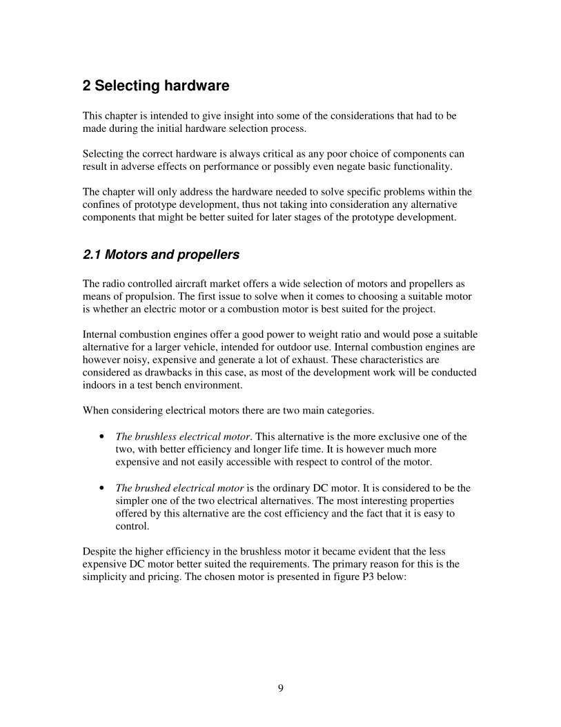
Despite the higher efficiency in the brushless motor it became evident that the less expensive DC motor better suited the requirements. The primary reason for this is the simplicity and pricing. The chosen motor is presented in figure P3 below:

10

Figure P3 is showing the motor chosen for the thesis.

The name of the motor is GWS EPS350CS and it includes

gearing with the ratio of 5.33:1.

Propellers come in many different sizes and shapes. A suitable propeller for the motor and its purpose of use is the Master airscrew size 10x6, two of the propellers being left rotating (pulling) and two of them right rotating (pushing). Technical data of the motors is presented in appendix A.

11

2.2 Speed controllers

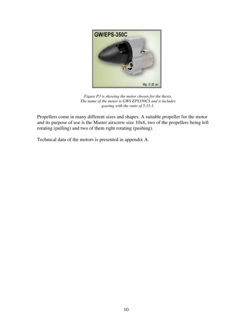
The power consumption in the motors is quite demanding. The maximum limit for the current in one motor is 10 A. and to avoid having to handle this current directly with any computer unit (this would require a considerable amount of electronics) it is possible to use a speed controller. This is a device that needs only a control signal from the computer unit and then adjusts the voltage to the motor accordingly. It can handle the high currents and is located between the power supply and the motor. An additional cable connected to the computer unit enables it to receive control information. The speed controller is shown in figure P4.

Figure P4 shows the speed controller GWS ICS-480 which

was used in the thesis. The picture also shows the heat sink

and connectors.

Technical data of the speed controller is presented in appendix B.

2.3 Eyebot

The eyebot control card is a small computer card fitted with multiple analogue and digital inputs and outputs. Additionally, there are multiple servo and other connection possibilities. It is based on the 32-bit Motorola 68332 controller and is mainly used in various robotic applications. The eyebot card enables a user to get access to an integrated system ready to implement without having to worry about various interfaces during the development work. One problem is that the card is too big and heavy to carry onboard the flying model. It is better to make the model as light as possible and then carry as many batteries as possible to increase the fly time. To enable this it becomes essential for the eyebot card to be stationary and connected to the sensors onboard the model by cable. As mentioned earlier this is a prototype development solution and will seriously cause limited mobility of the flying model. At later stages it will become necessary to find an onboard solution using a microcontroller. This will however not be considered in this report.

12

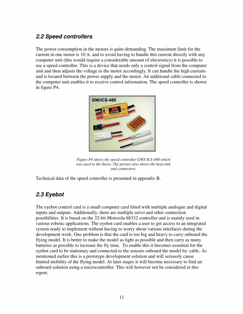
It is possible to program the eyebot card with either assembler or C/C++ programming language. All the programs that are associated to the report will be presented as C code. A picture of the eyebot card is presented below in figure P5.

Figure P5 shows the front side of the eyebot card used

during the development of the flying model.

Technical data of the eyebot card is presented in appendix C.

2.4 Gyrocube

It is always desirable to have as many sensors as possible when a measurement is being conducted. This enables a user to cross reference measurements and use statistical methods to increase the accuracy in a result. In this project however, some of the key features were simplicity and low cost. In order to uphold these original terms an attempt is going to be done using MEMS accelerometers and gyros only. The gyrocube is a MEMS gyro and accelerometer sensor package. It outputs an analogue signal and is assembled with multiple sensors to cover six degrees of freedom. Additionally to this it is very small and light weight, making it ideal for the project. The gyrocube is going to be mounted in the centre of the flying model. Communication with the eyebot cards AD converter will be via cable. Technical data of the gyrocube sensor package is presented in appendix D.

13

2.5 Anti alias filter

As an analogue signal is being sampled it is critical to remember that it is only possible to regenerate a signal containing frequencies up to half the frequency that was used to sample the signal. It is usually referred to as the Nyquist frequency. This means that if frequencies above the Nyquist frequency are not removed from the signal before the sampling, it will be impossible to determine whether the signal obtained after the sampling is the correct signal or if it is distorted by frequencies that are too high. This distortion is generally referred to as alias distortion. The solution for this problem is to implement an anti alias filter. More of this can be read about in signals and systems by Oppenheim, Willsky [1]. Preliminary tests suggested that the eyebot card would only be able to sample the sensor signal with a rate in the order of 20Hz. At the same time the motors generate vibrations in the order of 2 KHz. It is clear that an anti alias filter with a cut off frequency in the order of 10 Hz has to be implemented. The design of the filter is presented in chapter 4.3.1.

2.6 Power supply and cabling

Due to the demanding power consumption in the motors, a small battery will only be able to sustain flight for a few minutes. In order to prolong trials and to avoid interruptions caused by having to charge the batteries it would be desirable to work with a power supply that can sustain a long fly time. One solution for this is to use many small batteries and changing them when depleted. Small and efficient batteries however are expensive, and the number of batteries needed to enable work to be conducted without interruptions makes this alternative difficult to motivate when considering the cost. Another possibility is to use a ground based power supply during the development work. The speed controllers however can only be connected to a battery with a maximum voltage of 9.6V. This limits the selection of batteries since the majority of batteries larger than 10Ah come in 12V or 24V. It is difficult or expensive to obtain a 9.6V battery of this size with the maximum current properties needed for the project. The decision was made to use a large battery together with a voltage regulator. This solution allows the battery to be of any size and voltage above 9.6V with the regulator ensuring that the voltage does not exceed the limit. The motor chosen and described in section 2.1 has a maximum current limit of 10A. With four motors it is essential that the voltage regulator is able to deliver a maximum of 40A. With this current running in cables next to the signal cables it is important not to overlook the shielding. The signal can easily become contaminated from electrical and magnetic fields. This is closely described in teoretisk elektroteknik by Gunnar Peterson [2]. The design of the power supply is presented in chapter 4.3.2.

14

2.7 Chapter summary

When selecting the hardware presented in this chapter only a principal solution of the given problem was considered. One of the biggest limitations in the thesis is time. The selection of hardware was made with the intention to minimize time used to set up a working prototype. Hopefully this will result in enough time remaining to develop a working control system for the prototype. Such a solution could then be transferred to an integrated model where more research would be conducted to optimize material choices and design.

15

3 Problem analysis This chapter will discuss the theoretical and practical issues regarding the control functions involved in the thesis. The modelling, and the methods of control, will be explained separately with motivated methodology.

3.1 Modelling the system

In order to simulate a system it is necessary to create a mathematical model of the system dynamics. It is important to remember that a model is an attempt to describe the dynamics in a simplified way. A high order model will better describe the real system than a low order model. It is however not always desirable to make a model of the highest possible order, since this is very demanding and often requires a lot of calculations. A frequently used procedure is to start with a low order model. This is often satisfactory for control purposes and in the event of the model proving to be inadequate, the model order is increased. In the sub chapters, all models will have the order of three or less. This may seem as a very crude level to choose, but it turns out that it is often enough for control purposes. The modelling procedure is described closely in Modellbygge och simulering by Ljung, Glad [3].

16

3.1.1 Modelling the motors and propellers

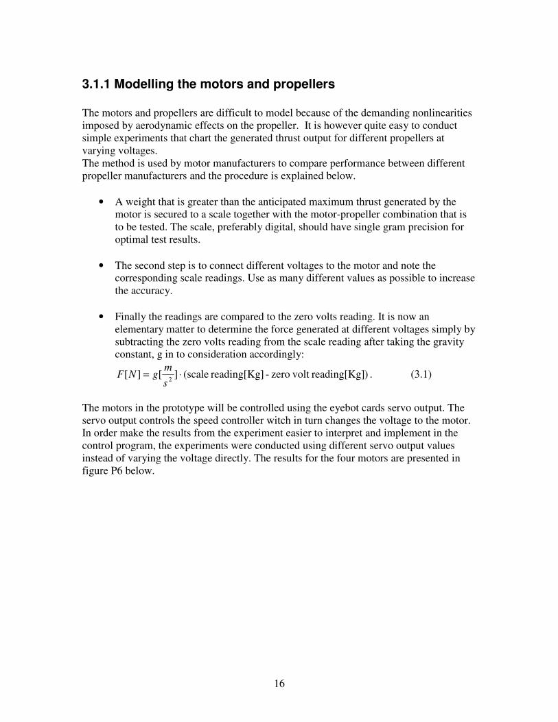
The motors and propellers are difficult to model because of the demanding nonlinearities imposed by aerodynamic effects on the propeller. It is however quite easy to conduct simple experiments that chart the generated thrust output for different propellers at varying voltages. The method is used by motor manufacturers to compare performance between different propeller manufacturers and the procedure is explained below.

• A weight that is greater than the anticipated maximum thrust generated by the motor is secured to a scale together with the motor-propeller combination that is to be tested. The scale, preferably digital, should have single gram precision for optimal test results.

• The second step is to connect different voltages to the motor and note the corresponding scale readings. Use as many different values as possible to increase the accuracy.

• Finally the readings are compared to the zero volts reading. It is now an elementary matter to determine the force generated at different voltages simply by subtracting the zero volts reading from the scale reading after taking the gravity constant, g in to consideration accordingly:

)]reading[Kg volt zero - ]reading[Kg scale(][][2

⋅=s

mgNF . (3.1)

The motors in the prototype will be controlled using the eyebot cards servo output. The servo output controls the speed controller witch in turn changes the voltage to the motor. In order make the results from the experiment easier to interpret and implement in the control program, the experiments were conducted using different servo output values instead of varying the voltage directly. The results for the four motors are presented in figure P6 below.

17

Figure P6 shows the thrust produced at different servo

outputs, each motor represented with a different colour.

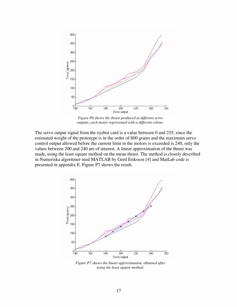
The servo output signal from the eyebot card is a value between 0 and 255, since the estimated weight of the prototype is in the order of 800 grams and the maximum servo control output allowed before the current limit in the motors is exceeded is 240, only the values between 200 and 240 are of interest. A linear approximation of the thrust was made, using the least square method on the mean thrust. The method is closely described in Numeriska algoritmer med MATLAB by Gerd Eriksson [4] and MatLab code is presented in appendix E. Figure P7 shows the result.

Figure P7 shows the linear approximation, obtained after

using the least square method.

18

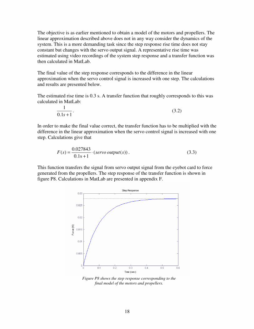
The objective is as earlier mentioned to obtain a model of the motors and propellers. The linear approximation described above does not in any way consider the dynamics of the system. This is a more demanding task since the step response rise time does not stay constant but changes with the servo output signal. A representative rise time was estimated using video recordings of the system step response and a transfer function was then calculated in MatLab. The final value of the step response corresponds to the difference in the linear approximation when the servo control signal is increased with one step. The calculations and results are presented below. The estimated rise time is 0.3 s. A transfer function that roughly corresponds to this was calculated in MatLab:

11.0

1

+s. (3.2)

In order to make the final value correct, the transfer function has to be multiplied with the difference in the linear approximation when the servo control signal is increased with one step. Calculations give that

))( (10.1s

0.027843)( soutputservosF ⋅

+= . (3.3)

This function transfers the signal from servo output signal from the eyebot card to force generated from the propellers. The step response of the transfer function is shown in figure P8. Calculations in MatLab are presented in appendix F.

Figure P8 shows the step response corresponding to the

final model of the motors and propellers.

19

3.1.2 Physical modelling

Physical modelling uses a different approach compared to the modelling procedure explained in previous sub chapter. Instead of relying on experimental or other data, it uses known physical properties to deduce theoretical models. In order to fully be able to simulate the prototype it is essential to produce two models. One that corresponds to the properties of the prototype when being subject for the altitude control, and the other one for the angle control (pitch and bank). The two models will be explained separately in this chapter.

3.1.2.1 Altitude model

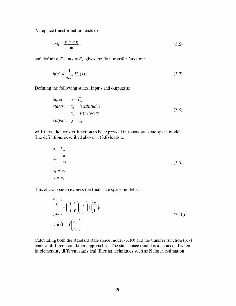
One of the main objectives with physical modelling is to simplify the physical properties of the system that is to be modelled. The idea being that one obtains a much simpler model which, serves to explain the main characteristics of the real system. The simplest possible way to simplify the prototype is to regard of it as a mass which is subject to two forces, the gravity and the force from the motors. Figure P9 shows the details.

Figure P9 shows the principal physical characteristics of

the prototype, when it is subject for the altitude control.

When considering the simplified system described above it is not as difficult to derive a transfer function as when considering the entire real system. Most of the physical properties are however described in the simplified model. The calculations are presented below: From Newton’s second law it is known that

⇔⋅=− ammgF (3.4)

m

mgF

dt

dv −=⇔ . (3.5)

h

v

m

F

mg

F (force from motors) v (velocity) m (mass) h (altitude) g (gravity)

20

A Laplace transformation leads to

m

mgFhs

−=2 , (3.6)

and defining mFmgF =− gives the final transfer function:

)(1

)(2

sFms

sh m= . (3.7)

Defining the following states, inputs and outputs as

1

2

1

:

)( :

)( :

:

xyoutput

velocityvx

altitudehxstates

Fuinput m

=

=

=

=

(3.8)

will allow the transfer function to be expressed in a standard state space model. The definitions described above in (3.8) leads to

1

21

2

xy

xx

m

ux

Fu m

=

=

=

=

•

•

(3.9)

This allows one to express the final state space model as:

( )

=

+

=

•

•

2

1

2

1

2

1

0 1

1

0

0

1

0

0

x

xy

ux

x

x

x

(3.10)

Calculating both the standard state space model (3.10) and the transfer function (3.7) enables different simulation approaches. The state space model is also needed when implementing different statistical filtering techniques such as Kalman estimation.

21

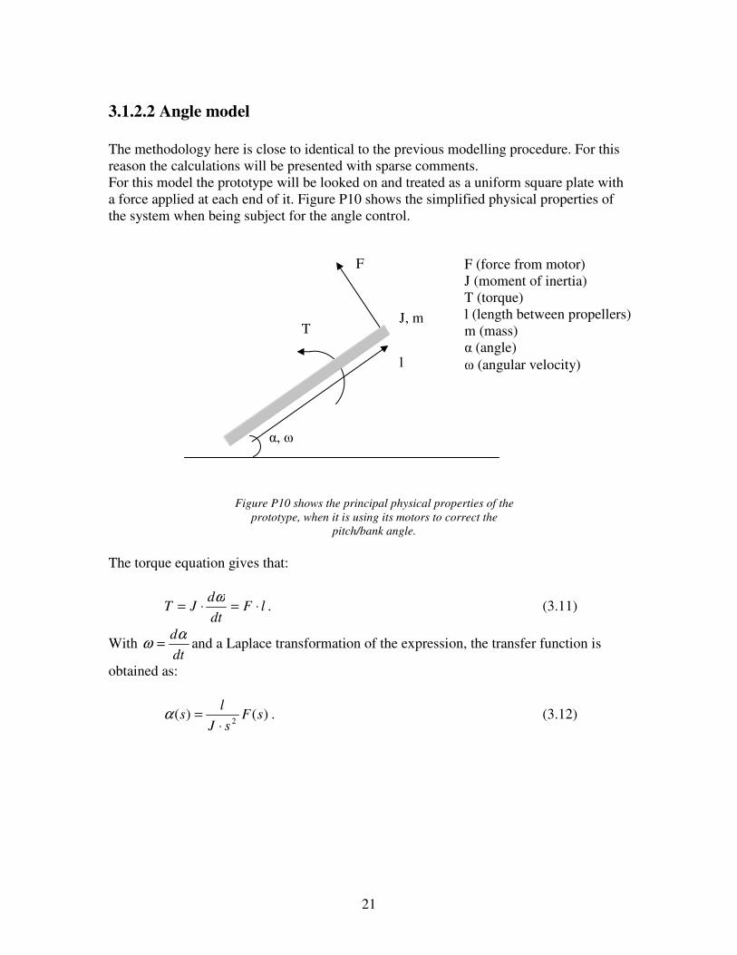
3.1.2.2 Angle model

The methodology here is close to identical to the previous modelling procedure. For this reason the calculations will be presented with sparse comments. For this model the prototype will be looked on and treated as a uniform square plate with a force applied at each end of it. Figure P10 shows the simplified physical properties of the system when being subject for the angle control.

Figure P10 shows the principal physical properties of the

prototype, when it is using its motors to correct the

pitch/bank angle.

The torque equation gives that:

lFdt

dJT ⋅=⋅=

ω. (3.11)

With dt

dαω = and a Laplace transformation of the expression, the transfer function is

obtained as:

)()(2

sFsJ

ls

⋅=α . (3.12)

l

T

α, ω

F

J, m

F (force from motor) J (moment of inertia) T (torque) l (length between propellers) m (mass) α (angle)

ω (angular velocity)

22

Defining states, input, and outputs as:

1

2

1

:

)( :

)( :

:

xyoutput

velocityvx

altitudehxstates

Fuinput m

=

=

=

=

(3.13)

Gives the final state space model:

( )

=

+

=

•

•

2

1

2

1

2

1

0 1

0

0

1

0

0

x

xy

u

J

lx

x

x

x

(3.14)

In order for this model to be valid it is important that the prototype is built with the centre of gravity at the same level as the propellers. This will result in a prototype that reacts in a linear manner and will not be affected by gravity when controlling the angle.

23

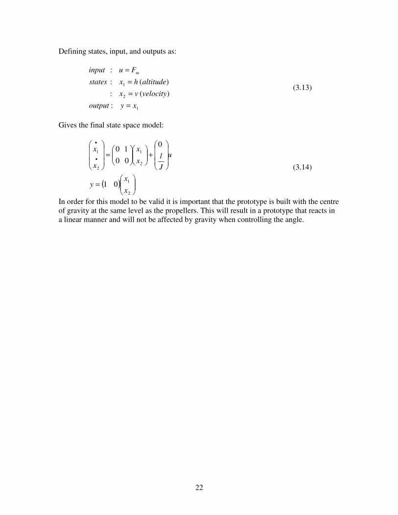
If the centre of gravity is not at the same level as the propellers the following (figure P11) principal physical properties will better describe the prototype:

Figure P11 shows the simplified system if the prototype is

not built with the centre of gravity at the same level as the

propellers.

It is clear that gravity will affect the transfer function and introduce nonlinear properties. Analogous to previous calculations the transfer function is now given by:

)sin()()(22

ααJs

dgsF

Js

ls −= . (3.14)

l

T

α,ω

F

J

m

mg

d

F (force) J (moment of inertia) T (torque) d (centre of gravity offset) l (length between propellers) m (mass) α (angle)

ω (angular velocity)

24

3.2 System control

It is often desirable to solve a control problem analytically. This facilitates the possibilities to ensure a certain degree of quality concerning the control properties. It is however often difficult to accomplish this because of various reasons. In our system there are many nonlinearities, and although there has been a considerable amount of research done in this area and good literature is to be found on the subject (such as Nonlinear systems by Khalil [5]), the many nonlinearities affecting the system at the same time makes it very difficult to present an analytical solution. One way to overcome the difficulties of analytical calculations is to simulate the system. The fundamental idea is to decide the control parameters for the system through the simulation and then transfer them to the prototype. The critical part here it to make a sufficiently adequate model of the dynamics in the system. This is discussed in section 3.1. All the simulation work has been conducted in Simulink. This is a signal processing tool that is a part of MatLab.

3.2.1 Altitude control

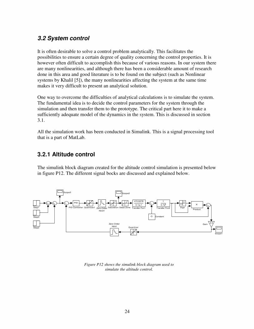
The simulink block diagram created for the altitude control simulation is presented below in figure P12. The different signal bocks are discussed and explained below.

Zero-Order

Hold1

Zero-Order

Hold

1

0.7s 2

Transfer Fcn2

4*0.0278

0.1s+1

Transfer Fcn1

Step3

Step2

Step1 Sign

Scope3Scope2

Scope1

SaturationQuantizer1

Quantizer

Product

PID

PID Controller

0.5Gain

Dead Zone

-C- Constant

Figure P12 shows the simulink block diagram used to

simulate the altitude control.

25

• PID The system was simulated using an ideal PID controller. This an approximation of what is going to be possible to implement in the control program. It is however difficult to simulate the exact properties of the real system.

• Quantizer1 and zero order hold1 The control program is going to calculate an output value and hold this value until the next one is calculated. This is represented by the quantizer and zero order hold blocks.

• Saturation In order to limit the output from the angle control, the saturation block was added. This block simulates a maximum and minimum limit of the output allowed to be used as altitude control signal.

• Transfer function1 and transfer function2 These are the models of the motors with propellers and the prototype. The models are described in previous section 3.1, equation (3.3) and (3.7).

• Constant

The constant block simulates the effects of the gravity.

• Sign, product, gain

These blocks are logical function blocks outputting zero when the signal otherwise would be smaller than zero. This enables simulation of the ground.

• Quantizer and zero order hold The altitude is measured using the analogue inputs in the eyebot card. The quantizer and zero order hold bocks simulate an AD converter sampling a value and holding it until the next value is sampled. The altitude measurement is assumed to have the resolution of one centimetre.

• Step1, step2, step3

These blocks are input steps put together to provide an input to the system.

• Scope1, scpoe2, scope3

The scope blocks are used to extract graphs of system performance. Preliminary tests suggested that the eyebot card would be able to sample the sensor signal with a rate in the order of 20Hz. This corresponds to a sample time of 0.05s, which was used throughout the simulation. Results from the simulation are presented in figure P13, P14 and P15 below.

26

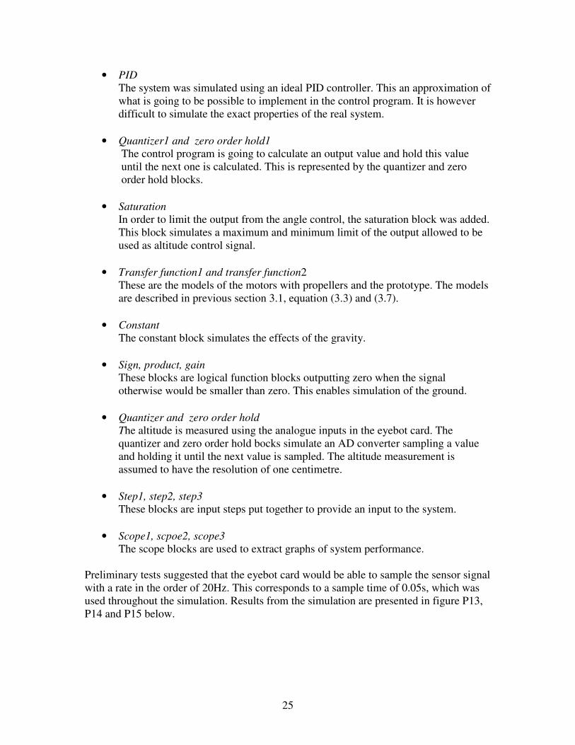
Figure P13 shows a graph of the input step. It is important

to ensure control robustness both in descending and

ascending situations. For this reason several steps were put

together to create the input.

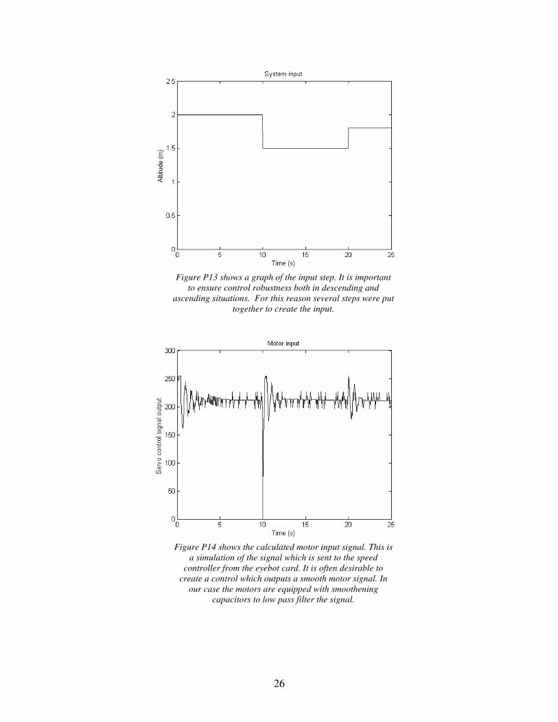
Figure P14 shows the calculated motor input signal. This is

a simulation of the signal which is sent to the speed

controller from the eyebot card. It is often desirable to

create a control which outputs a smooth motor signal. In

our case the motors are equipped with smoothening

capacitors to low pass filter the signal.

27

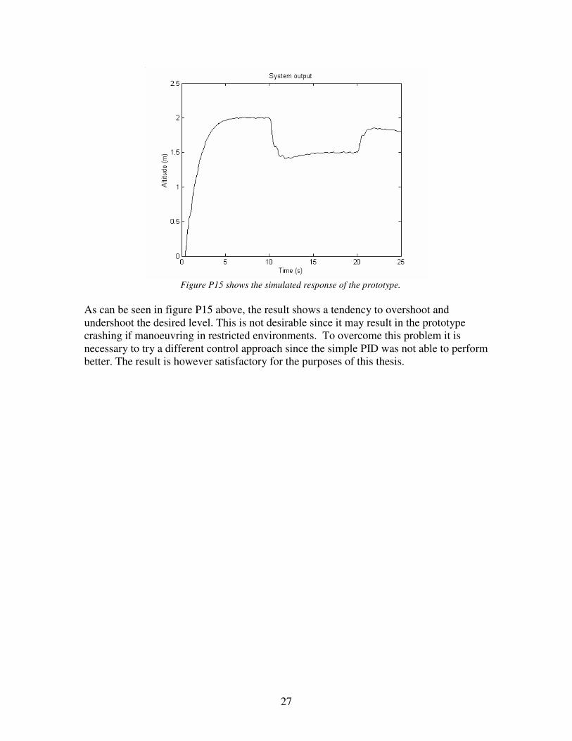
Figure P15 shows the simulated response of the prototype.

As can be seen in figure P15 above, the result shows a tendency to overshoot and undershoot the desired level. This is not desirable since it may result in the prototype crashing if manoeuvring in restricted environments. To overcome this problem it is necessary to try a different control approach since the simple PID was not able to perform better. The result is however satisfactory for the purposes of this thesis.

28

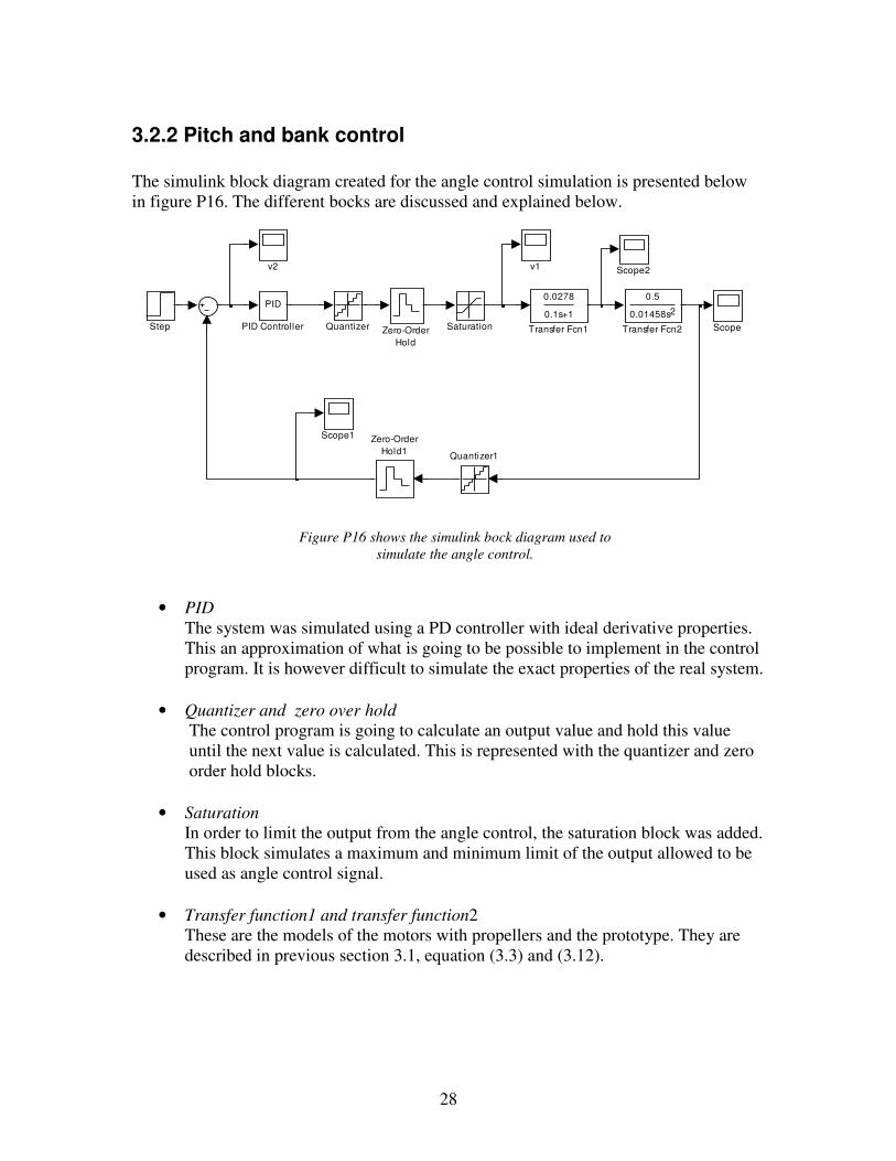
3.2.2 Pitch and bank control

The simulink block diagram created for the angle control simulation is presented below in figure P16. The different bocks are discussed and explained below.

v2 v1

Zero-Order

Hold1

Zero-Order

Hold

0.5

0.01458s 2

Transfer Fcn2

0.0278

0.1s+1

Transfer Fcn1Step

Scope2

Scope1

ScopeSaturation

Quantizer1

Quantizer

PID

PID Controller

Figure P16 shows the simulink bock diagram used to

simulate the angle control.

• PID The system was simulated using a PD controller with ideal derivative properties. This an approximation of what is going to be possible to implement in the control program. It is however difficult to simulate the exact properties of the real system.

• Quantizer and zero over hold The control program is going to calculate an output value and hold this value until the next value is calculated. This is represented with the quantizer and zero order hold blocks.

• Saturation In order to limit the output from the angle control, the saturation block was added. This block simulates a maximum and minimum limit of the output allowed to be used as angle control signal.

• Transfer function1 and transfer function2 These are the models of the motors with propellers and the prototype. They are described in previous section 3.1, equation (3.3) and (3.12).

29

• Quantizer1 and zero order hold1 The angle is measured using the analogue inputs in the eyebot card. The quantizer1 and zero order hold1 blocks simulate an AD converter sampling a value and holding it until the next value is sampled.

• Step1

This block provides an input step to the system.

• Scope, scope1, scope2, v1, v3

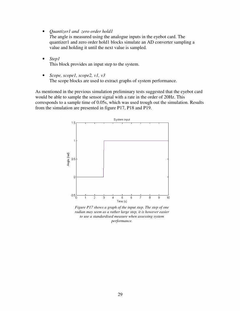
The scope blocks are used to extract graphs of system performance. As mentioned in the previous simulation preliminary tests suggested that the eyebot card would be able to sample the sensor signal with a rate in the order of 20Hz. This corresponds to a sample time of 0.05s, which was used trough out the simulation. Results from the simulation are presented in figure P17, P18 and P19.

Figure P17 shows a graph of the input step. The step of one

radian may seem as a rather large step, it is however easier

to use a standardised measure when assessing system

performance.

30

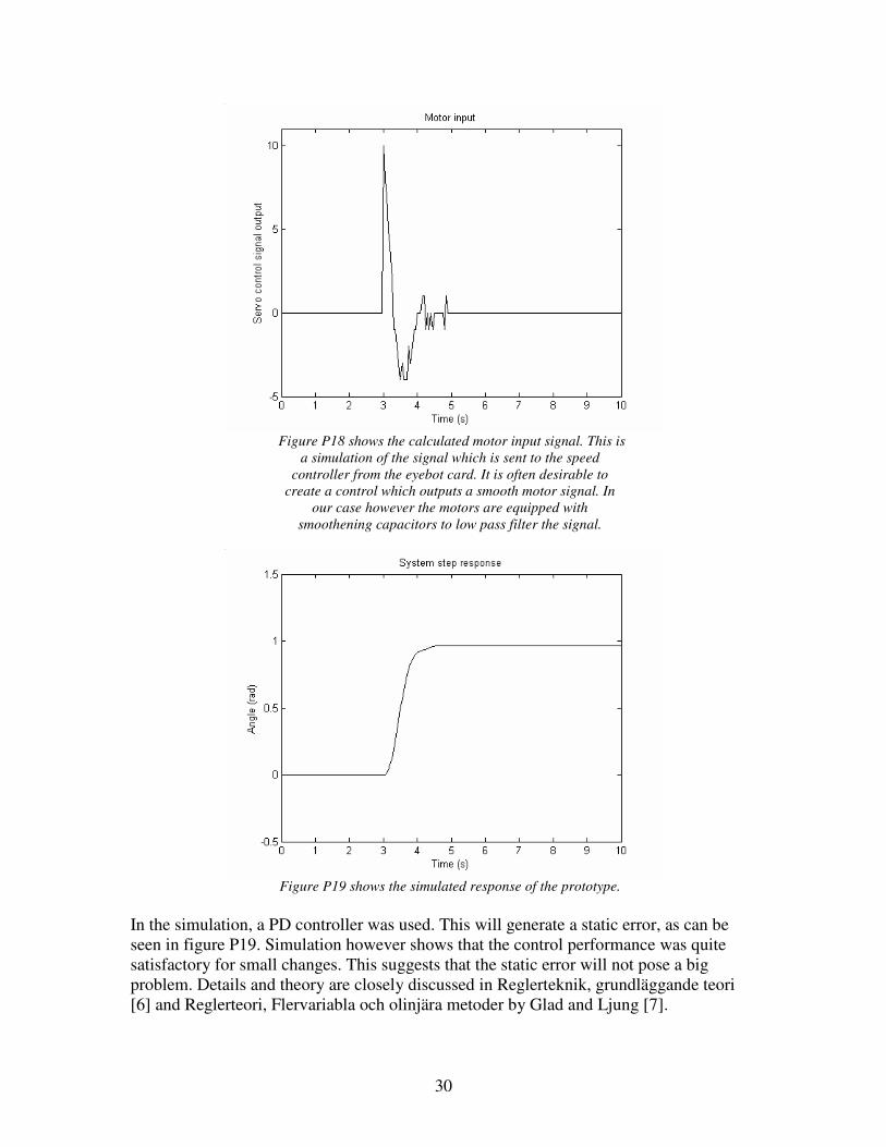
Figure P18 shows the calculated motor input signal. This is

a simulation of the signal which is sent to the speed

controller from the eyebot card. It is often desirable to

create a control which outputs a smooth motor signal. In

our case however the motors are equipped with

smoothening capacitors to low pass filter the signal.

Figure P19 shows the simulated response of the prototype.

In the simulation, a PD controller was used. This will generate a static error, as can be seen in figure P19. Simulation however shows that the control performance was quite satisfactory for small changes. This suggests that the static error will not pose a big problem. Details and theory are closely discussed in Reglerteknik, grundläggande teori [6] and Reglerteori, Flervariabla och olinjära metoder by Glad and Ljung [7].

31

3.2.3 Yaw control

Any vehicle equipped with a rotating motor will be affected by the torque generated in the motor. If the torque is large enough to negatively affect vehicle control, it has to be counteracted. There are different ways solve this problem, as can be seen in the helicopter tail rotor or adjustment of aileron and side rudders when increasing the throttle in a propeller airplane. The prototype in the thesis will be equipped with four motors with propellers, two of them rotating clockwise and two counter clockwise. Propellers rotating in the same direction will be mounted diagonally across the prototype to counteract the torque generated. The main idea for yaw control is to use the torque in a controlled manner. If the prototype needs to rotate to the left, a small part of the thrust used to maintain altitude is shifted to the right turning motors. The total amount of thrust is maintained while the torque from the right turning motors overcomes the torque generated by the left turning motors. The prototype will be affected by this surplus of torque generated by the right turning motors and react by rotate to the left. The yaw control was not simulated since the main focus was directed towards the angle and altitude control. The intension is to use a simple on off control and experimentally obtain all variables, such as amount of thrust shifted between the motors and control thresholds.

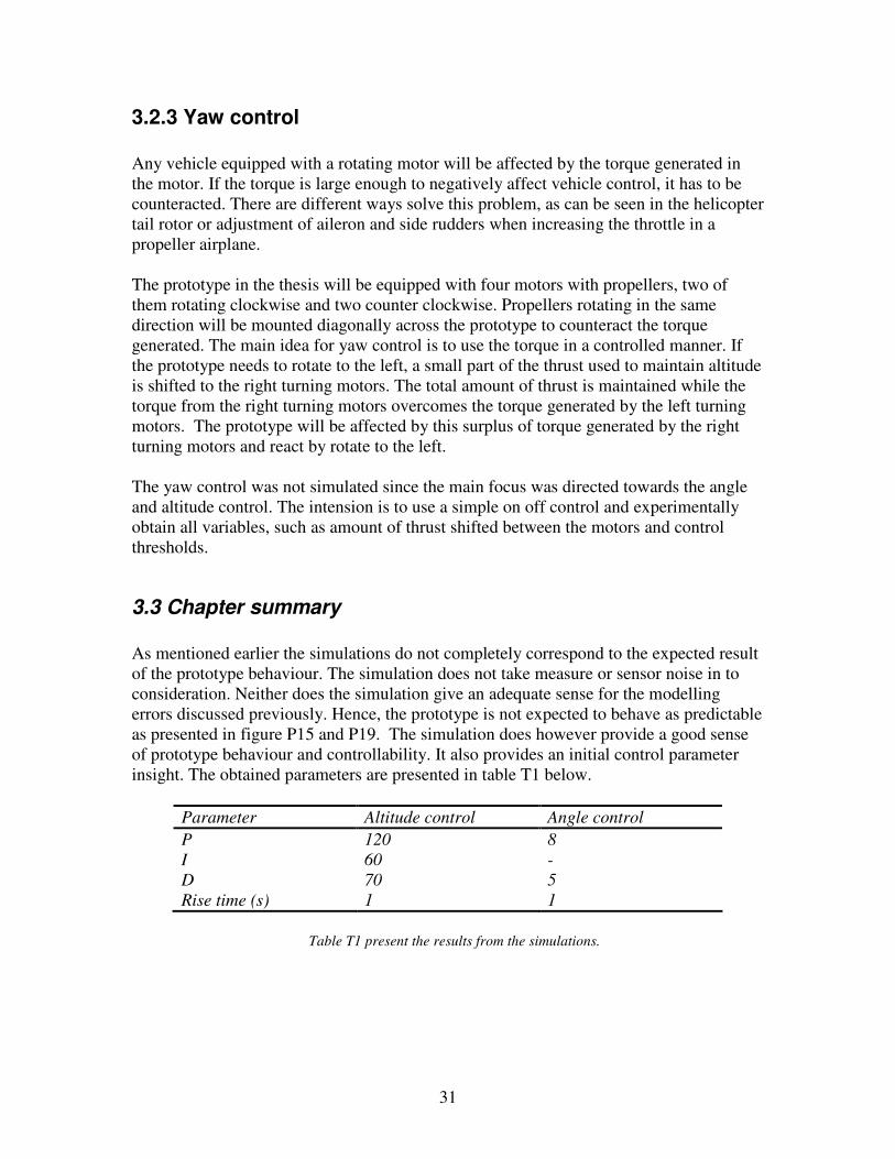
3.3 Chapter summary

As mentioned earlier the simulations do not completely correspond to the expected result of the prototype behaviour. The simulation does not take measure or sensor noise in to consideration. Neither does the simulation give an adequate sense for the modelling errors discussed previously. Hence, the prototype is not expected to behave as predictable as presented in figure P15 and P19. The simulation does however provide a good sense of prototype behaviour and controllability. It also provides an initial control parameter insight. The obtained parameters are presented in table T1 below.

Parameter Altitude control Angle control

P 120 8

I 60 -

D 70 5

Rise time (s) 1 1

Table T1 present the results from the simulations.

32

4 Hardware design This chapter will present the hardware components designed and built for the project. As mentioned earlier in chapter 2 most hardware components presented here are only to be used during the development of the prototype and further development is necessary to integrate them to an onboard solution.

4.1 Materials

There is a great range of selection when it comes to building materials for the prototype. A presentation of the materials considered for the prototype is given below.

• Polystyrene

This material offers good filling properties. It is however fragile, and to ensure satisfactory results it must be used together with other materials that provides a protective cover and load bearing properties.

• Carbon fibre

The carbon fibre has many advantageous properties such as rigidity and low weight. It is however quite expensive and difficult to obtain in wanted dimensions. This often results in, that one has to compromise with the design and adapt the design to available dimensions, or alternatively face the high cost connected to the manufacturing of wanted dimensions.

• Balsa wood

Balsa has the advantage of being very light weight. The fragile property of balsa however makes it more suitable to use in covering applications than to use in any load bearing structures.

• Pine wood

The pine wood offers a very good strength to price ratio and a fair strength to weight ratio. Further more, pine beams are easy to work with and come in many different dimensions. All the properties mentioned above contribute to make it the most popular building material in model airplane circuits.

• Plywood For the same reasons as pine wood, the plywood is a popular building material amongst model airplane builders. It is quite heavy and is therefore only interesting in thicknesses around a few millimetres.

There is an endless range of materials suitable for prototype construction. The materials discussed above are only a small selection chosen mainly for the availability and cost properties they pose.

33

4.2 Building the model

In order to evaluate different building techniques, two prototypes were built for the project. The two building techniques offer various advantages and are presented below.

4.2.1 Prototype A

The first prototype made, was built using a polystyrene body. The polystyrene was shaped with a foam cutter made of an electrically heated wire that is held tight in a frame. The fragile property of polystyrene however makes it critical to use a core and cover material with better properties in order to add strength and protection. For this, pine wood beams and three millimetres thick plywood was used to construct the load-bearing structure. Thin balsa wood sheets were glued on to the polystyrene to provide a strong and smooth surface. This building technique will result in a lightweight and rigid construction with a durable outer shell. It is however better suited for larger constructions since it is quite demanding to shape polystyrene in small dimensions. Pictures of the model are shown below in figure P20, P21 and P22.

Figure P20 gives an overall presentation of the prototype A.

50 cm

34

Figure P21 shows a better view of the electrical component

compartment. This picture also shows the polystyrene and

plywood layers inside of the compartment.

Figure P22shows one of the engine mounts.

10 cm

10 cm

35

4.2.2 Prototype B

The second building technique is not as extensive as the one described above. The main idea here is to use pine wood beams and thin plywood only, to create a simple but functional prototype. The result is not as rigid as in the technique used for prototype A. It is however particularly suited for prototype construction since the result is relatively lightweight and easy to build and above all, easy to modify. It is often the case that something is overlooked during the initial planning and that the design has to be changed to compensate for this. Details regarding prototype B are further discussed in section 6.2.

4.3 Control unit

The control unit consists of all hardware components that are stationary and only are to be used during the development of the prototype. A presentation of the various components is given below.

• Power supply

The power supply will only be used early in the development work and is later to be replaced by onboard batteries. The design of the power supply is discussed in section 4.3.2.

• Eyebot card The eyebot control card is a small computer card fitted with multiple analogue and digital inputs and outputs. It is further discussed in section 2.3. This component will later be replaced with an integrated onboard microcontroller.

• Anti alias filter

For reasons discussed in section 2.5 there is a need for an anti alias filter. Even though further development should not change the electrical properties of the filter significantly, it should be made smaller and lighter before used onboard the AFV. The design of the filter is presented in chapter 4.3.1

36

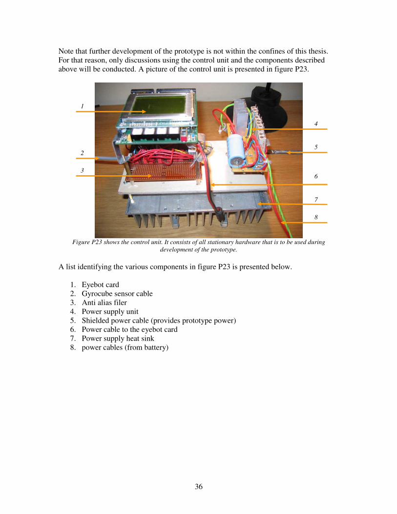
Note that further development of the prototype is not within the confines of this thesis. For that reason, only discussions using the control unit and the components described above will be conducted. A picture of the control unit is presented in figure P23.

Figure P23 shows the control unit. It consists of all stationary hardware that is to be used during

development of the prototype.

A list identifying the various components in figure P23 is presented below.

1. Eyebot card 2. Gyrocube sensor cable 3. Anti alias filer 4. Power supply unit 5. Shielded power cable (provides prototype power) 6. Power cable to the eyebot card 7. Power supply heat sink 8. power cables (from battery)

1

2

3

4

5

7

8

6

37

4.3.1 Anti alias filter

Preliminary tests on the eyebot card suggested that the sensor signal would be sampled with a maximum rate in the order of 20Hz. At the same time the motors generate vibrations in the order of 2 KHz. For reasons discussed in section 2.5 it is clear that an anti alias filter with a cut off frequency in the order of 10 Hz has to be implemented. There are mainly two different types of analogue filters, the passive filter which is built by using passive components only (inductors, capacitors and resistors), and the active filter, built around an amplifier (often an OP amplifier). The low cut off frequency in the given problem would result in very large and heavy inductors in the passive filter and is consequently not suitable for the task. In an active filter solution there is no need for inductors when implementing a simple low pass filter, see figure P24.

Figure P24 shows the schematics of the second order

Butterworth filter used as the anti alias filter. In a low pass implementation G1 and G3 are resistors and G2 and G4 are capacitors. There is no need for inductors and the result is a light weight and easy to implement filter. Calculations for the filter components are presented in appendix J.

G1

G2

G3

G4

+

_

OPA1014

38

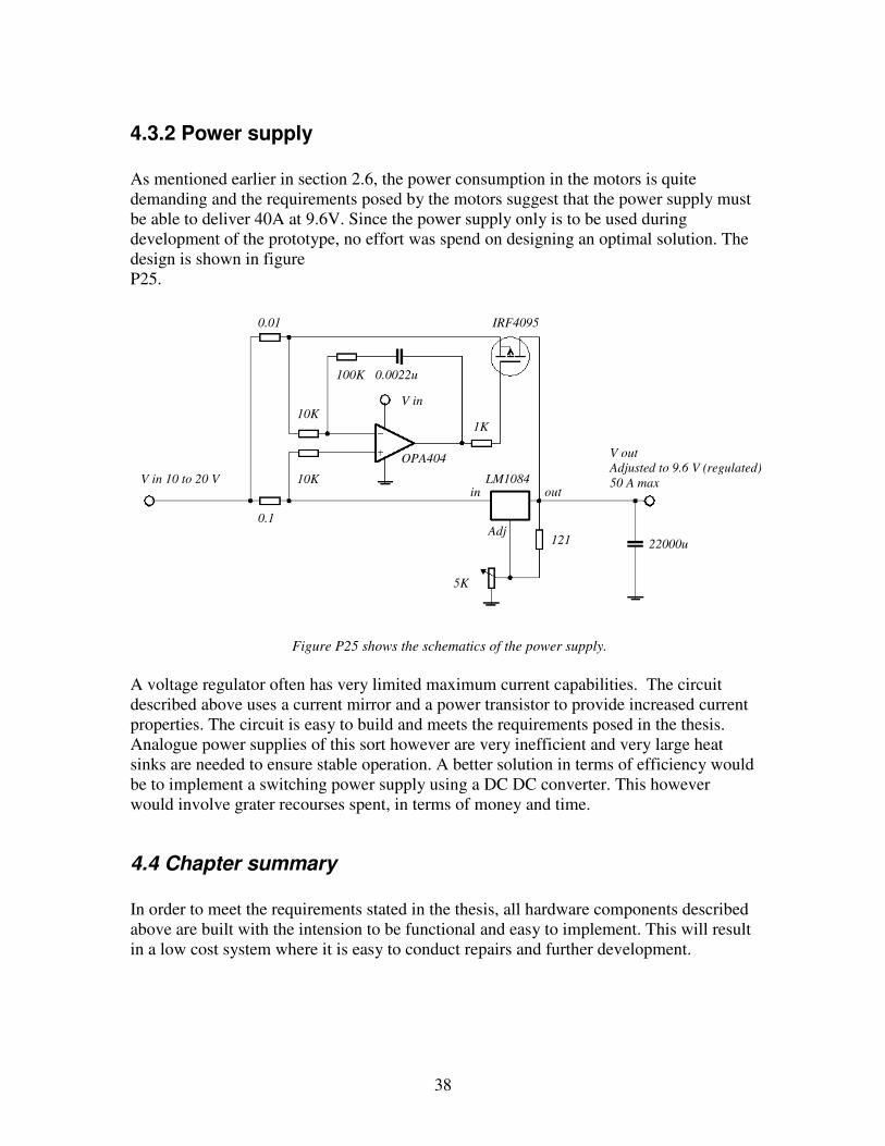
4.3.2 Power supply

As mentioned earlier in section 2.6, the power consumption in the motors is quite demanding and the requirements posed by the motors suggest that the power supply must be able to deliver 40A at 9.6V. Since the power supply only is to be used during development of the prototype, no effort was spend on designing an optimal solution. The design is shown in figure P25.

Figure P25 shows the schematics of the power supply.

A voltage regulator often has very limited maximum current capabilities. The circuit described above uses a current mirror and a power transistor to provide increased current properties. The circuit is easy to build and meets the requirements posed in the thesis. Analogue power supplies of this sort however are very inefficient and very large heat sinks are needed to ensure stable operation. A better solution in terms of efficiency would be to implement a switching power supply using a DC DC converter. This however would involve grater recourses spent, in terms of money and time.

4.4 Chapter summary

In order to meet the requirements stated in the thesis, all hardware components described above are built with the intension to be functional and easy to implement. This will result in a low cost system where it is easy to conduct repairs and further development.

10K

10K

0.01

0.1

100K 0.0022u

1K

121

V in 10 to 20 V

V out

Adjusted to 9.6 V (regulated)

50 A max

V in

out

Adj

in LM1084

5K

22000u

IRF4095

OPA404

39

5 Software design Theoretical solutions that are intended for incorporation with any software application offer many alternatives when it comes to method of implementation. This chapter will discuss methods used in the thesis and in some cases compare different solutions.

5.1 Overall software design

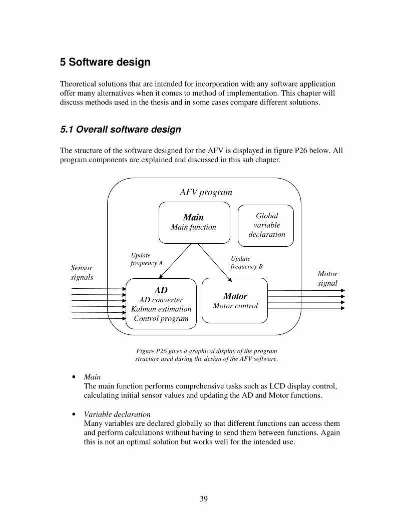
The structure of the software designed for the AFV is displayed in figure P26 below. All program components are explained and discussed in this sub chapter.

Figure P26 gives a graphical display of the program

structure used during the design of the AFV software.

• Main

The main function performs comprehensive tasks such as LCD display control, calculating initial sensor values and updating the AD and Motor functions.

• Variable declaration

Many variables are declared globally so that different functions can access them and perform calculations without having to send them between functions. Again this is not an optimal solution but works well for the intended use.

Main Main function

AD AD converter

Kalman estimation

Control program

Sensor

signals

Update

frequency B

Motor Motor control

Update

frequency A

Global

variable

declaration

AFV program

Motor

signal

40

• AD

The AD function is updated regularly using a constant time interval. It samples the sensor signal and estimates states using a Kalman estimator. Desired state values subtracted to the estimated states pose an input to the control algorithm, which is also incorporated in this function.

• Motor

The motor function is updated regularly using a constant time interval, which may differ from the interval used to update the AD function. This contingency allows further control when deciding on how computer recourses should be distributed. The motor function uses the control values from the AD function to output a servo control signal, which is subsequently sent to the speed controllers.

41

5.2 Sensor bias

The ten bit AD converter in the eyebot card outputs a sampled sensor signal represented by an integer between 0 to1023. The midpoint value (512) represents zero sensor output. In order to extract useful data from the sensor it becomes essential to remove the DC part of the sampled signal. The removal of the DC part can be done using several different methods and a listing of the methods used in the thesis is presented below.

• Kalman filter estimator

The subject of Kalman theory is quite comprehensive and can be discussed extensively. In the thesis however, only considerations regarding the implementation has been made. The method and implementation is further discussed in section 5.3.

• High pass filter The basic idea here is to use digital filter theory to create a filter, which removes the DC part of the signal. Using the digital signal-processing tool, fdatool in MatLab, filter coefficients were created. A sample frequency of 20Hz was assumed and the cut off frequency was set to 0.01Hz. This resulted in a fourth order IIR (infinite impulse response) filter. Details of the implementation are more extensively discussed in appendix G. Details of the IIR filter can be found in Statistical Digital Signal processing and modelling by Monson H. Hayes [8].

• Removing the bias

This method is simpler than the previously mentioned methods and is best suited for sensor testing. It is fast and easy to implement and does not require demanding calculations. It is however inferior to the purpose of this thesis since it does not in any way consider the extensive problem of sensor drift. The method will generate a small error with each program cycle which will accumulate in time and generate a sensor error of considerable size. Details of the implementation are more extensively discussed in appendix H.

42

5.3 Kalman estimator

The Kalman estimator was used both to estimate the angle (pitch and bank) of the prototype and the sensor bias. The theory of Kalman filtering is, as mentioned earlier quite comprehensive and for this reason, only the basic calculations and the implementation will be discussed in the chapter. The discrete time Kalman filter equations are described in Optimal Filtering by Andersson and Moore [9], and are, together with the initializations given below. Initializations:

The estimation error covariance matrix was initialized as

=

10

01P . (5.1)

The estimation vector was defined as a two state vector where the first state is the angle (bank) of the vehicle and the other is the sensor bias. It was initialized as

=

−

∧

biassensor estimated

01kkx . (5.2)

Initializing the angle as zero means that it is essential that the AFV starts in a level position since the initial angle of the AFV will be interpreted as zero in the program. Gain update:

( ) 1

11

−

−−+= v

T

kk

T

kkk RCCPCPK (5.3)

Updating the measurement:

−+=

−

∧

−

∧∧

11 kkkkkkkk xxx CyK (5.4)

( )1−

−=kkkkk

PCKIP (5.5)

Time update:

kkkkkBuA xx +=

∧

+

∧

1 (5.6)

k=k+1: T

w

T

kkkkGGRAAPP +=

+1 (5.7)

vR and wR were experimentally obtained.

43

The equations (5.1) to (5.7) were used together with a state space model describing the relationship between the wanted states. Calculations are shown below. The states are defined as:

velocityangularinputsensorgyrou

biasx

anglex

2

1

==

=

=

(5.8)

With this follows that:

02

21

=

+−=

•

•

x

uxx (5.9)

Now the state space model can be expressed in the standard form

Cxy

BuAxx=

+=∧

as

( )xy

uxx

01

0

1

00

10

=

+

−=

•

(5.10)

Note that the state vector (5.2) above only consists of two states. The reason for this is that the theory presented above is only intended to describe one degree of freedom (bank). The symmetrical property of the prototype enables an identical implementation for the pitch axis. The implementation is further described in appendix I.

44

5.4 PID design

In order to evaluate different PID implementations, two principally different PID designs were tested in the thesis. These two designs were implemented in several control situations, controlling different states. A large amount of testing was conducted to optimize the control performance. The two PID solutions are presented below.

• PID A

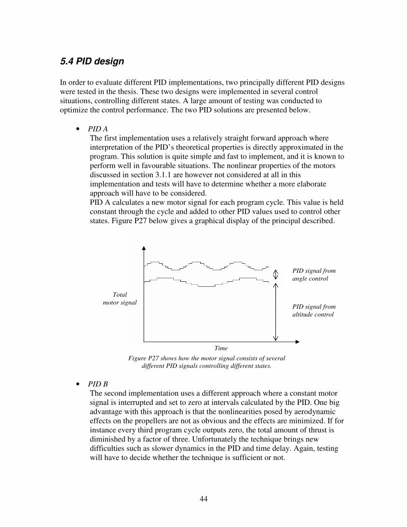
The first implementation uses a relatively straight forward approach where interpretation of the PID’s theoretical properties is directly approximated in the program. This solution is quite simple and fast to implement, and it is known to perform well in favourable situations. The nonlinear properties of the motors discussed in section 3.1.1 are however not considered at all in this implementation and tests will have to determine whether a more elaborate approach will have to be considered. PID A calculates a new motor signal for each program cycle. This value is held constant through the cycle and added to other PID values used to control other states. Figure P27 below gives a graphical display of the principal described.

Figure P27 shows how the motor signal consists of several

different PID signals controlling different states.

• PID B

The second implementation uses a different approach where a constant motor signal is interrupted and set to zero at intervals calculated by the PID. One big advantage with this approach is that the nonlinearities posed by aerodynamic effects on the propellers are not as obvious and the effects are minimized. If for instance every third program cycle outputs zero, the total amount of thrust is diminished by a factor of three. Unfortunately the technique brings new difficulties such as slower dynamics in the PID and time delay. Again, testing will have to decide whether the technique is sufficient or not.

Time

Total

motor signal

PID signal from

angle control

PID signal from

altitude control

45

The C code implementation is further discussed in appendix K and more of PID implementations can be read of in Embedded Robotics [10] by Thomas Bräunl.

5.5 Chapter summary

It is important to mention that the software solutions described above only consider a principal solution to the given problems. To achieve wanted results, one has to adapt to the problem with is to be solved by combining several techniques and modifying standard methods.

46

6 Implemented system The initial component evaluation resulted in a system being put together using the most promising solutions. It is presented in this chapter together with discussions regarding each system component.

6.1 Software

In order to obtain a functional program, the software structure described in section 5.1 was used. This structure has the advantage of being very functional and allowing a user to distribute computer recourses in order to optimise computer usage. The AD function was updated with the frequency of 20 Hz and the motor function with the frequency of 100 Hz. This combination offers a well functional balance between computer capability and program continuity. The extensive problem of estimating states was carried out using two different techniques. The methods are discussed below.

• The pitch and bank angle estimation was made by using a Kalman estimator. The technique was also used to estimate the sensor bias and is further discussed in section 5.3.

• The yaw angle was obtained by implementing a digital high pass filter to remove the DC part of the signal. This allowed the use of a simple integrator to estimate the yaw angle. More of the technique can be read of in section 5.2.

Testing made it evident that the best control algorithm was provided by PID control B, discussed in section 5.4. A more elaborate version was however implemented where the angle acceleration was used to simulate the effects of a faster PID response. Further, a moving average filter was implemented to smooth out the motor signal. The implementation is shown in appendix K.

47

6.2 Hardware

The greater part of hardware selection and design was made in the initial evaluation. Hence, many of the hardware components used in the prototype have been presented in previous chapters. A detailed list of the hardware in question is however presented below.

• Motors are discussed in section 2.1

• Speed controllers are presented in section 2.2

• Sensors used for orientation and stabilization are discussed in section 2.4

• Control unit components are presented in chapter 2 and in section 4.3

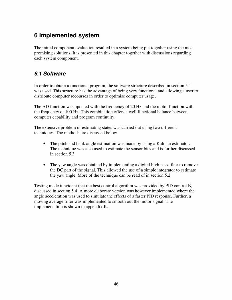
• Model is presented below The prototype was made using building technique B described in section 4.2.2. Pictures describing the prototype in detail are presented below in figures P28, P29, P30 and P31.

Figure P28 gives an overview of the prototype including the

motors and propellers, the body and sensors.

48

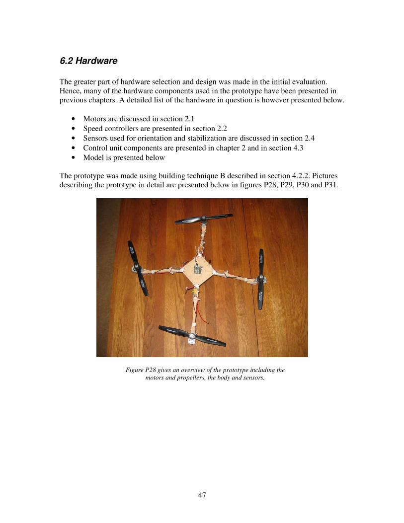
Picture P29 shows the angle of the arms, giving the

prototype a centre of gravity better suiting the modelling

results discussed in section 3.1.2.2.

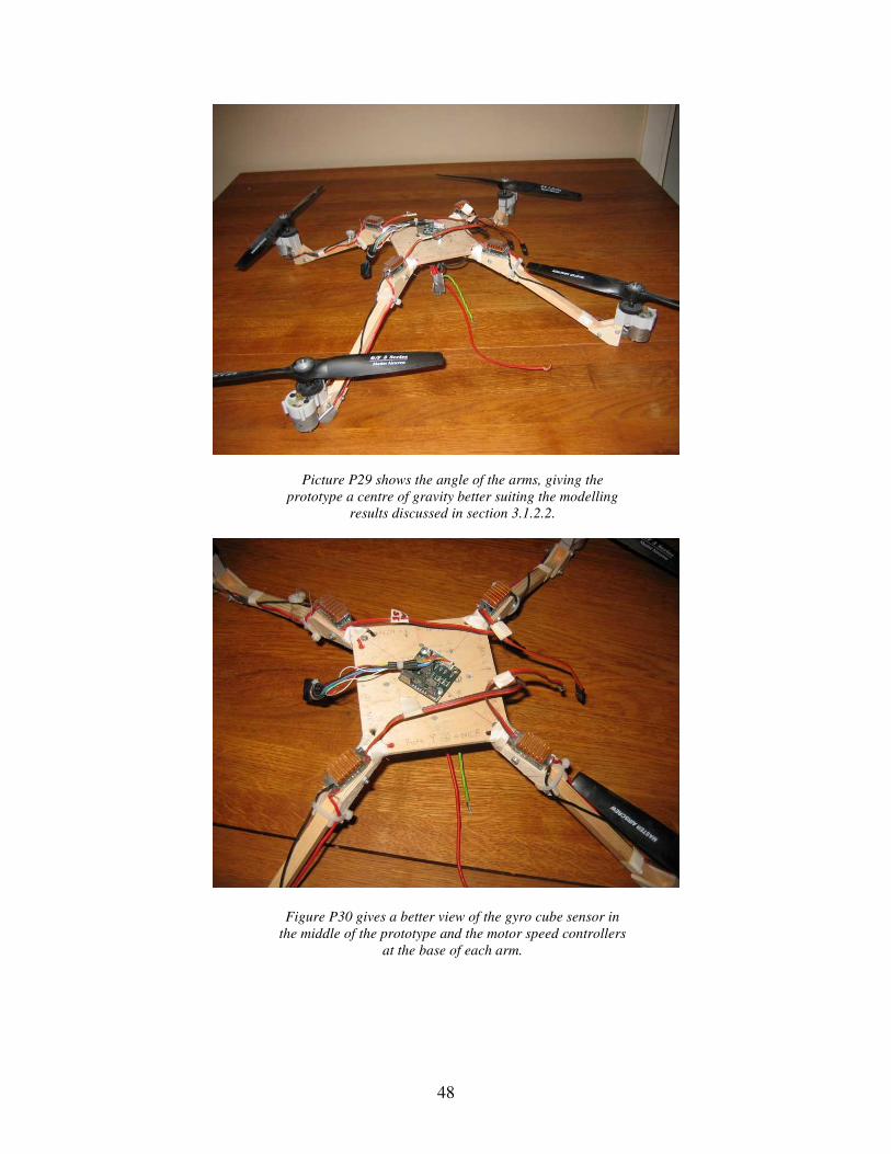
Figure P30 gives a better view of the gyro cube sensor in

the middle of the prototype and the motor speed controllers

at the base of each arm.

49

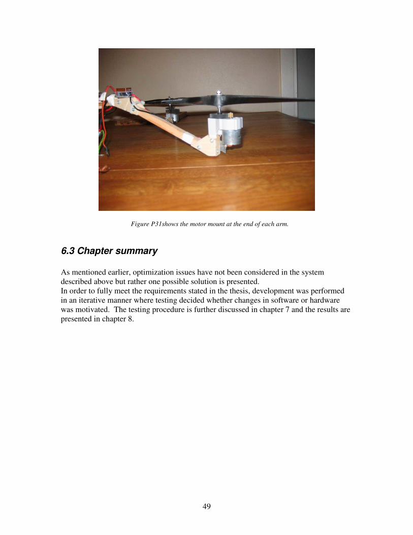
Figure P31shows the motor mount at the end of each arm.

6.3 Chapter summary

As mentioned earlier, optimization issues have not been considered in the system described above but rather one possible solution is presented. In order to fully meet the requirements stated in the thesis, development was performed in an iterative manner where testing decided whether changes in software or hardware was motivated. The testing procedure is further discussed in chapter 7 and the results are presented in chapter 8.

50

7 Testing In order to fully being able to evaluate a certain subsystems performance, a practical approach was assumed where testing decided whether changes had to be made. This chapter will discuss testing procedures for different subsystems and in some cases methods of rating the result.

7.1 Hardware testing

Since proper functionality of the prototype is critical, all hardware components were individually tested before integrated in the system. The subchapters below describe the testing procedure.

7.1.1 Power supply

The power supply was tested together with the battery pack and the main part of the test was performed during the modelling of the motors and propellers described in section 3.1.1. Since the power consumption in the motors is quite demanding it was important to make sure that the power supply was able to maintain a certain voltage when all four motors were connected. The test was performed simply by measuring the voltage from the power supply while running the motors at different speeds.

51

7.1.2 Anti alias filter

The anti alias filter has the function to remove unwanted signal elements (this is further discussed in chapter 2.5). In order to test the functionality of the filter, a signal generator and a frequency analyser was used. The signal generator was connected to the filer input and set to perform a frequency sweep ranging from 0.01 Hz to 30 KHz. In order to further simulate the gyro cube signal a peak to peak value of 1.5V was used and a dc offset of 2.5V was added to the frequency sweep. The Frequency sweep signal is shown in picture P32 below.

Figure P32 shows the frequency sweep used to simulate the

anti alias filter input signal in the prototype.

The output of the filter was monitored and recorded in the frequency analyser. Here it was ensured that the filter performed correctly by not letting any unwanted signals elements (frequencies above the filter cut off frequency) passing through the filter.

7.1.3 Motors and propellers

The motors and propellers were extensively tested during the modelling phase described in chapter 3.1.1. Apart from the obvious modelling purposes described in that chapter the goal of the test was also to ensure proper functionality in the propeller and motor combination in question. This was achieved by ensuring that the amount of thrust was at a satisfactory level and that no voltage or current limits were exceeded.

52

7.1.4 Gyro cube

Testing of the accelerometers in the gyro cube was performed by measuring gravity in all three axes (x, y, z). The output was monitored trough the eyebot card and it was ensured that the measurement was constant and equal in size between the three axes. The gyros in the gyro cube were tested only for functionality by turning the gyro cube in different directions and monitoring the output on the eyebot card.

7.2 Software testing

The software was tested with respect to the control performance and was carried out in an iterative manner where testing indicated how the control parameters were to be adjusted. Each of the control algorithms used to control the model in different degrees of freedom were tested separately and the testing is described in the chapter below.

7.2.1 Pitch and bank control testing

When the model is held in a stationary position in the air (hovering), each of the motors ideally generate one fourth of the thrust needed to sustain a certain altitude. Additionally to this altitude trust, a small amount of thrust is continually added or subtracted in each motor by the pitch and bank control in order to compensate for, amongst other things non ideal properties in the motors and thereby to keep the model at a right angle. When testing the pitch and bank control, an ideal altitude thrust was simulated in two of the motors. This was achieved by suspending the model in the propellers of two diagonally opposing motors. An altitude thrust was then applied on the two remaining motors. This allowed testing to be performed in one axis at the time in a controlled manner with actual motor speeds used in real flight. The pitch and bank control signal was then added to the altitude thrust and the ability to maintain at a certain angle was observed. Picture P33 illustrates the procedure.

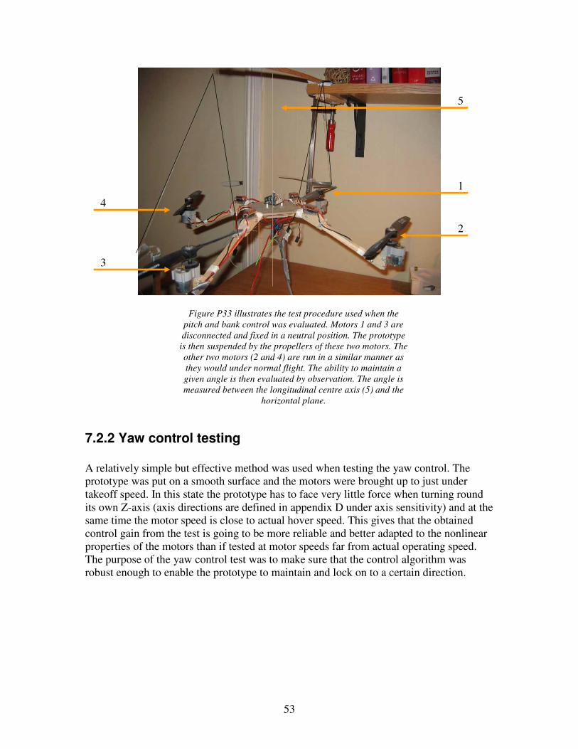
53

Figure P33 illustrates the test procedure used when the

pitch and bank control was evaluated. Motors 1 and 3 are

disconnected and fixed in a neutral position. The prototype

is then suspended by the propellers of these two motors. The

other two motors (2 and 4) are run in a similar manner as

they would under normal flight. The ability to maintain a

given angle is then evaluated by observation. The angle is

measured between the longitudinal centre axis (5) and the

horizontal plane.

7.2.2 Yaw control testing

A relatively simple but effective method was used when testing the yaw control. The prototype was put on a smooth surface and the motors were brought up to just under takeoff speed. In this state the prototype has to face very little force when turning round its own Z-axis (axis directions are defined in appendix D under axis sensitivity) and at the same time the motor speed is close to actual hover speed. This gives that the obtained control gain from the test is going to be more reliable and better adapted to the nonlinear properties of the motors than if tested at motor speeds far from actual operating speed. The purpose of the yaw control test was to make sure that the control algorithm was robust enough to enable the prototype to maintain and lock on to a certain direction.

1

3

2

4

5

54

7.2.3 Altitude control testing

The altitude control was not tested using a systematic procedure like the ones described above since the main focus was directed towards the angle and yaw control. It turned out that the yaw and angle control was not robust enough to sustain a stable position in the air. This involves that the altitude control was not possible to fully develop since the performance of it depends on the yaw and angle control being very robust. The plan however was to test the altitude control using a test fixture which only enabled the prototype to move along the z-axis (altitude direction). This could be achieved by mounting two parallel guide rails from floor to ceiling, allowing the prototype to slide up and down the rails but stopping it from twisting or turning in any direction.

7.3 Chapter summary

As previously mentioned, a very hands-on approach was assumed when testing the control performance and the hardware. Even though it in some cases may seem like the methodology was crude, it provided the results needed to make progress in the development of the control algorithms and verification of the hardware. Furthermore the methodology was non expensive, easy to adapt and produced the results needed to make critical conclusions regarding further development of the prototype. The results and conclusions can be read of in chapter 8.

55

8 Conclusions and summary This final chapter will summarize all results and conclusions obtained during the development of the prototype. As previously mentioned, the final result was not robust enough to sustain autonomous flight. It turned out that the Pitch/bank and yaw control each performed not far from satisfactory but when tried together in actual flight the test nearly ended in catastrophic failure. In this test the altitude was controlled manually and the flight test could be terminated before the prototype crashed. There are several reasons for the prototype not performing in a robust manner. The most primary and obvious ones are presented below.

• Poor pitch/bank angle measurement when the motors were running. Since the angle measurement worked very well with the motors turned off it can be claimed with some certainty that the problem is caused due to poor anti alias filter performance. The filter used in the prototype is of a second order Butterworth type. The frequency roll off in this filter is not very steep and if the filter order was to be increased, the frequency response would be improved and a significantly smaller part of unwanted signal elements would contaminate the signal.

• Poor pitch/bank control performance. The control algorithm was not far from satisfactory in it self, but as mentioned above the control performance was drastically reduced when used together with the yaw control in actual flight. There are several reasons for this where the most pronounced reason would be that the control algorithm should be more elaborate where the nonlinearities are considered to a greater extend. A proper methodology here would be to use the prototype model in a system identification method in order to obtain a good approximation of the model transfer function. This transfer function can be used to create an optimized control algorithm.

• Physical properties in model. A model witch further eliminates nonlinearities should be considered. The goal is to have a prototype with the centre of gravity at the same level as the propellers. This is to some extent discussed in section 6.2 and in section 3.1.2.2.

56

These conclusions are some of the main issues which have to be solved before autonomous flight could be possible. There are however several more issues which would all improve performance. Examples are presented below.

• Faster microprocessor or using multiple processors would improve control performance.

• Using lighter materials such as carbon fibre would improve control performance and prolong flight time.

• Replacing the DC motors with brushless electrical motors with better efficiency or with combustion engines would improve control performance and prolong flight time.

The above mentioned issues all address the actual flight stability problems experienced during the test of the prototype. The consequence of these dysfunctions is that the additional functionality of navigating and orientating in three dimensions have not been addressed or tested. The usage of accelerometers and gyros however will most likely not be sufficient due to sensor inaccuracy and drift, and the AFV will most probably have to be fitted with additional sensors such as IR, GPS and UV. Given these results one could argue that it is very difficult to create a fully functional autonomous flying vehicle when restricted with the limitations stated in the beginning of the thesis. It is however most likely possible to develop an AFV system given that all the suggested improvements were to be implemented. If the cost of the development is included, these improvements still impose a very low cost increase compared to that one of purchasing existing AFV systems today. Hence the final conclusion has to be that this type of low cost AFV systems poses a very interesting issue for further development where significant economical and functional gains can be made.

57

8.1 Issues for future development

This subchapter will summarize all issues which are subject for further development.

• Adding sensors. This issue is further discussed in section 8.

• Improve the angle measurement when the motors are running. This issue is further discussed in section 8.

• Improve pitch/bank control. This issue in further discussed in section 8.

• Build a lighter prototype using more appropriate materials such as carbon fibre. This issue is further discussed in section8.

• Improve the prototype shape to better eliminate nonlinearities. This issue is further discussed in section 8.

• Replace motors to more efficient ones. This issue is further discussed in section 8.

• Implementing rotational matrices. It is not possible to fully deduce a position and direction only from integrating accelerometer and gyro data. Most likely the rotational matrices calculations have to be performed together with the usage of GPS and perhaps compass data, in order to fully being able to determine a position and direction in three dimensions.

• During the development of the software no consideration to the initial pitch/bank angle was made. This means that the initial sensor reading from the accelerometer was considered to be zero degrees, this is obviously not true. It is not far fetched to assume that the prototype could take off from a non level surface. The software should be improved so that an initial angle is calculated in relation to gravity. This technique will allow the prototype not to be limited to taking off from level platforms only.

58

References

Printed literature

[1] Alan V. Oppenheim Alan S. Willsky, 1997,

Signals and systems, Prentice Hall, second edition, ISBN 0-13-814757-4

[2] Gunnar Pettersson, 2002,

Teoretisk elektroteknik Stationära fenomen, Institutionen för teoretisk elektroteknik, KTH, tredje tryckningen

[3] Torkel Glad, Lennart Ljung, 2004, Modellbygge och simulering, Studentlitteratur, andra upplagan, ISBN 91-44-024443-6

[4] Gerd Eriksson, 2002,

Numeriska Algoritmer med MATLAB, Institutionen för numerisk analys och datologi, KTH

[5] Hassan K. Khalil, 2002, Nonlinear systems, Prentice Hall, third edition, ISBN 0-13-067389-7

[6] Torkel Glad, Lennart Ljung, 1998,

Reglerteknik, grundläggande teori, Studentlitteratur, andra upplagan, ISBN 91-44-17892-1

[7] Torkel Glad, Lennart Ljung, 2003,

Reglerteori, Flervariabla och olinjära metoder, Studentlitteratur, andra upplagan, ISBN 91-44-03003-7

[8] Monson H. Hayes, 1996,

Statistical digital signal processing and modelling, John Wiley & sons, Inc, ISBN 0-471-59431-8

[9] Brian D. O. Anderson, John B. Moore, 1979,

Optimal Filtering, Prentice Hall, first edition, ISBN 0-13-638122-7

[10] Thomas Bräunl 2003,

Embedded Robotics, Springer-Verlag Berlin Heidelberg New York, ISBN 3-540-03436-6

59

Internet pages

[W1] Air force technology, United Sates and NATO Air force technology home page

http://www.airforce-technology.com/projects/predator/ Date of visit: 17/8 2007 [W2] Draganfly,

RC toy and industrial RC manufacturer home page http://www.draganfly.com/

Date of visit: 17/8 2007 [W3] Rotomotion,

Manufactures and operates helicopter robots and aerial robotic systems and components http://www.rotomotion.com/downloads/tilt.c/

Date of visit: 17/8 2007 [W4] Maxim, Electronic component manufacturer

http://www.maxim-ic.com/appnotes.cfm/appnote_number/1795/ Date of visit: 17/8 2007

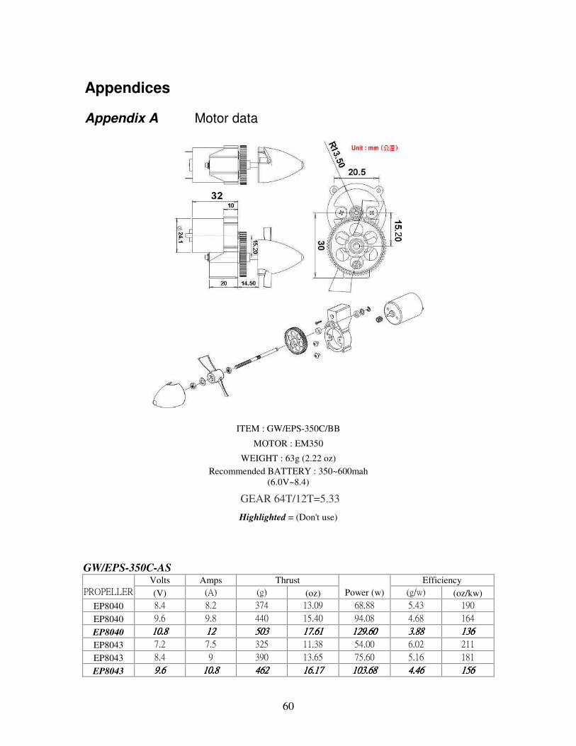
60

Appendices

Appendix A Motor data

ITEM : GW/EPS-350C/BB

MOTOR : EM350

WEIGHT : 63g (2.22 oz) Recommended BATTERY : 350~600mah

(6.0V~8.4)

GEAR 64T/12T=5.33

Highlighted = (Don't use)

GW/EPS-350C-AS Volts Amps Thrust Efficiency

PROPELLER (V) (A) (g) (oz) Power (w) (g/w) (oz/kw)

EP8040 8.4 8.2 374 13.09 68.88 5.43 190

EP8040 9.6 9.8 440 15.40 94.08 4.68 164

EP8040 10.810.810.810.8 12121212 503503503503 17.61 17.61 17.61 17.61 129.60 129.60 129.60 129.60 3.88 3.88 3.88 3.88 136136136136

EP8043 7.2 7.5 325 11.38 54.00 6.02 211

EP8043 8.4 9 390 13.65 75.60 5.16 181

EP8043 9.69.69.69.6 10.810.810.810.8 462462462462 11116.17 6.17 6.17 6.17 103.68 103.68 103.68 103.68 4.46 4.46 4.46 4.46 156156156156

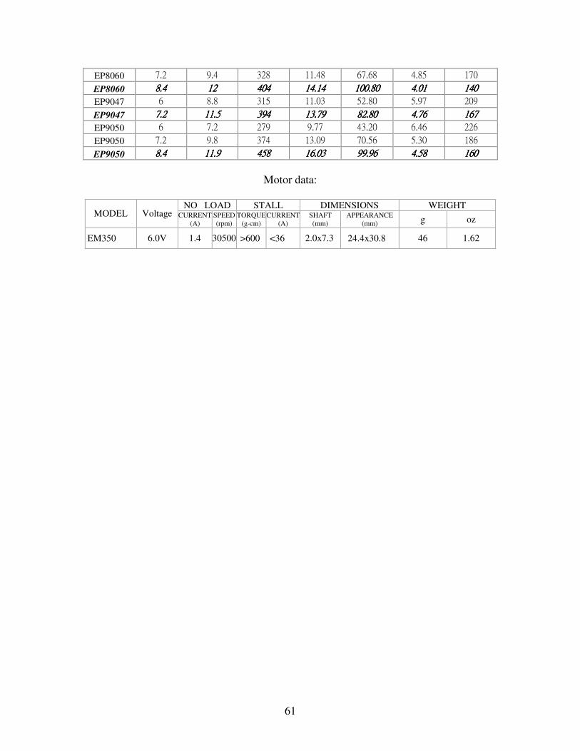
61

EP8060 7.2 9.4 328 11.48 67.68 4.85 170

EP8060 8.48.48.48.4 12121212 404404404404 14.14 14.14 14.14 14.14 100.80 100.80 100.80 100.80 4.01 4.01 4.01 4.01 140140140140

EP9047 6 8.8 315 11.03 52.80 5.97 209

EP9047 7.27.27.27.2 11.511.511.511.5 394394394394 13.79 13.79 13.79 13.79 82.80 82.80 82.80 82.80 4.76 4.76 4.76 4.76 167167167167

EP9050 6 7.2 279 9.77 43.20 6.46 226

EP9050 7.2 9.8 374 13.09 70.56 5.30 186

EP9050 8.48.48.48.4 11.911.911.911.9 458458458458 16.03 16.03 16.03 16.03 99.96 99.96 99.96 99.96 4.58 4.58 4.58 4.58 160160160160

Motor data:

NO LOAD STALL DIMENSIONS WEIGHT

MODEL Voltage CURRENT (A)

SPEED (rpm)

TORQUE (g-cm)

CURRENT (A)

SHAFT (mm)

APPEARANCE (mm) g oz

EM350 6.0V 1.4 30500 >600 <36 2.0x7.3 24.4x30.8 46 1.62

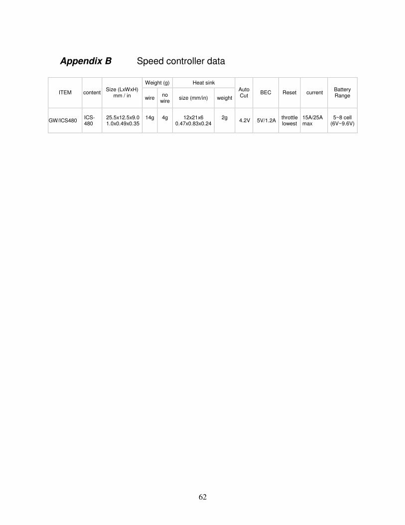
62

Appendix B Speed controller data

Weight (g) Heat sink

ITEM content Size (LxWxH)

mm / in wire no

wire size (mm/in) weight

Auto Cut

BEC Reset current Battery Range

GW/ICS480 ICS-480

25.5x12.5x9.0 1.0x0.49x0.35

14g

4g

12x21x6 0.47x0.83x0.24

2g

4.2V 5V/1.2A throttle lowest

15A/25A max

5~8 cell (6V~9.6V)

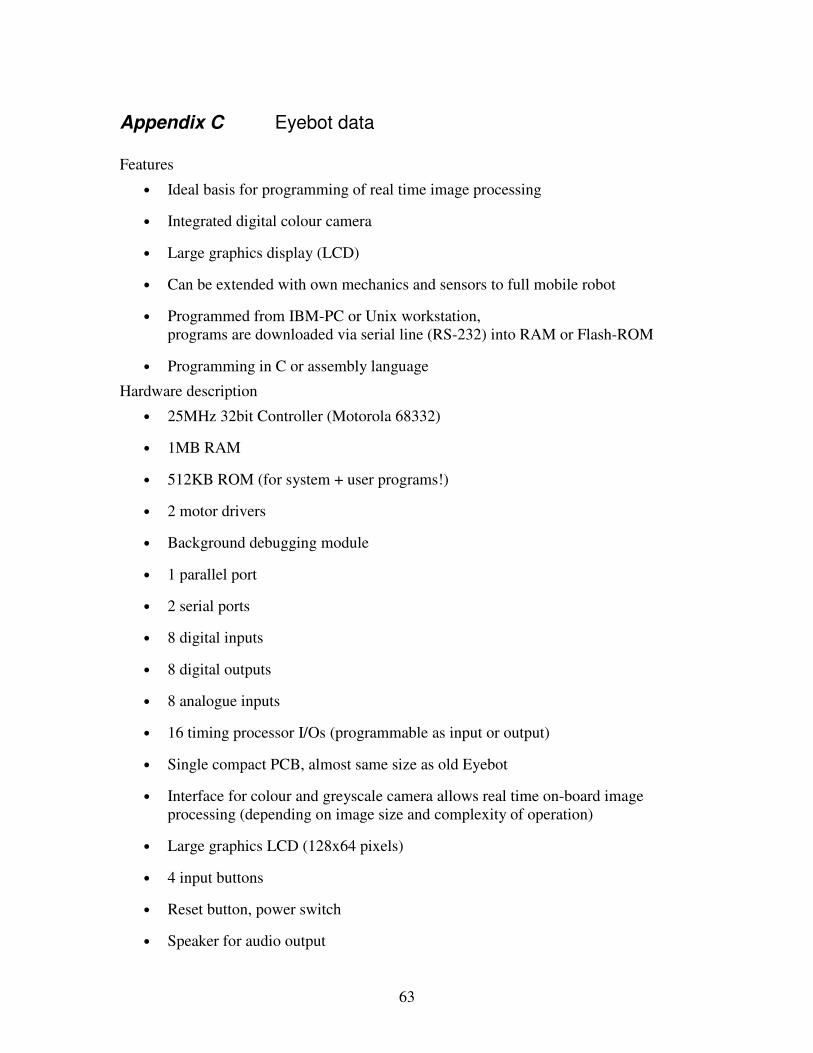
63

Appendix C Eyebot data

Features

• Ideal basis for programming of real time image processing

• Integrated digital colour camera

• Large graphics display (LCD)

• Can be extended with own mechanics and sensors to full mobile robot

• Programmed from IBM-PC or Unix workstation, programs are downloaded via serial line (RS-232) into RAM or Flash-ROM

• Programming in C or assembly language

Hardware description

• 25MHz 32bit Controller (Motorola 68332)

• 1MB RAM

• 512KB ROM (for system + user programs!)

• 2 motor drivers

• Background debugging module

• 1 parallel port

• 2 serial ports

• 8 digital inputs

• 8 digital outputs

• 8 analogue inputs

• 16 timing processor I/Os (programmable as input or output)

• Single compact PCB, almost same size as old Eyebot

• Interface for colour and greyscale camera allows real time on-board image processing (depending on image size and complexity of operation)

• Large graphics LCD (128x64 pixels)

• 4 input buttons

• Reset button, power switch

• Speaker for audio output

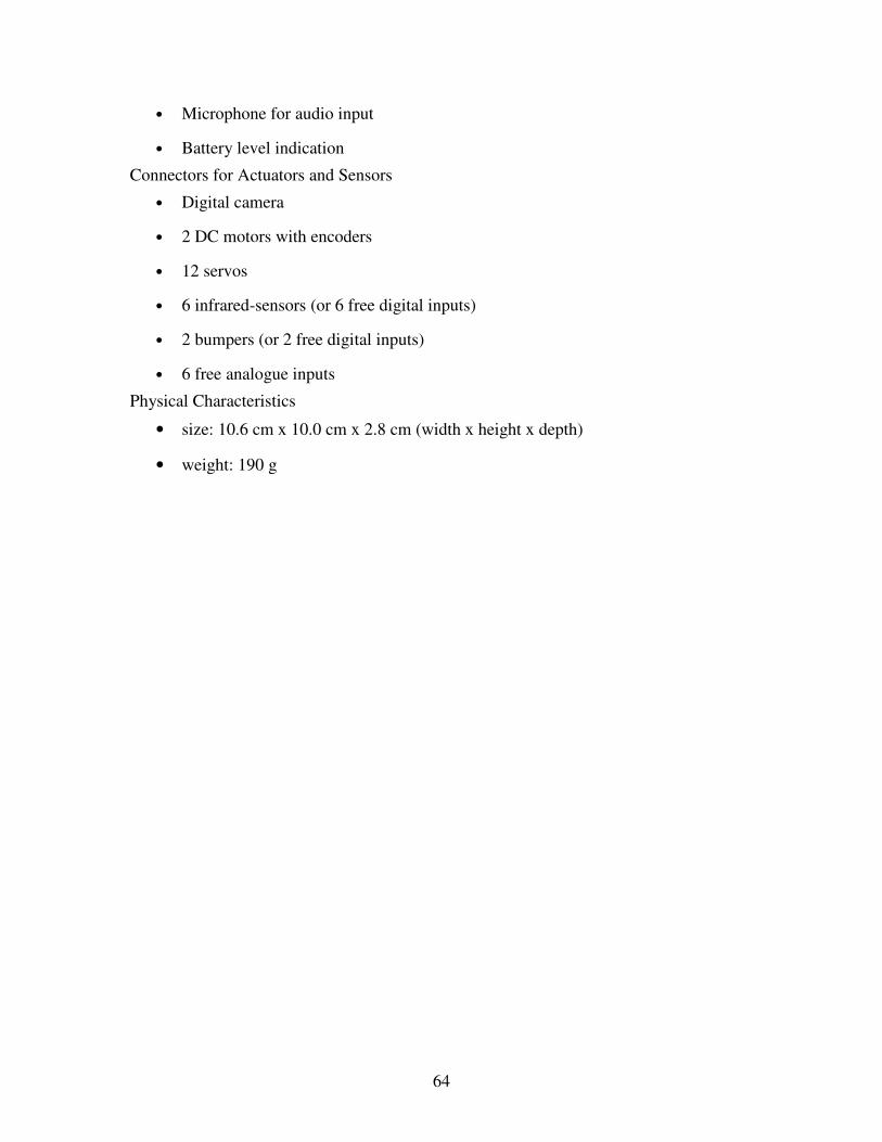
64

• Microphone for audio input

• Battery level indication

Connectors for Actuators and Sensors

• Digital camera

• 2 DC motors with encoders

• 12 servos

• 6 infrared-sensors (or 6 free digital inputs)

• 2 bumpers (or 2 free digital inputs)

• 6 free analogue inputs

Physical Characteristics

• size: 10.6 cm x 10.0 cm x 2.8 cm (width x height x depth)

• weight: 190 g

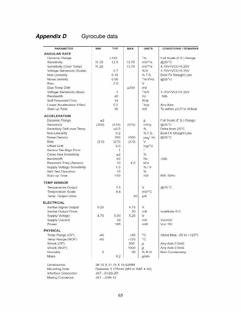
65

Appendix D Gyrocube data

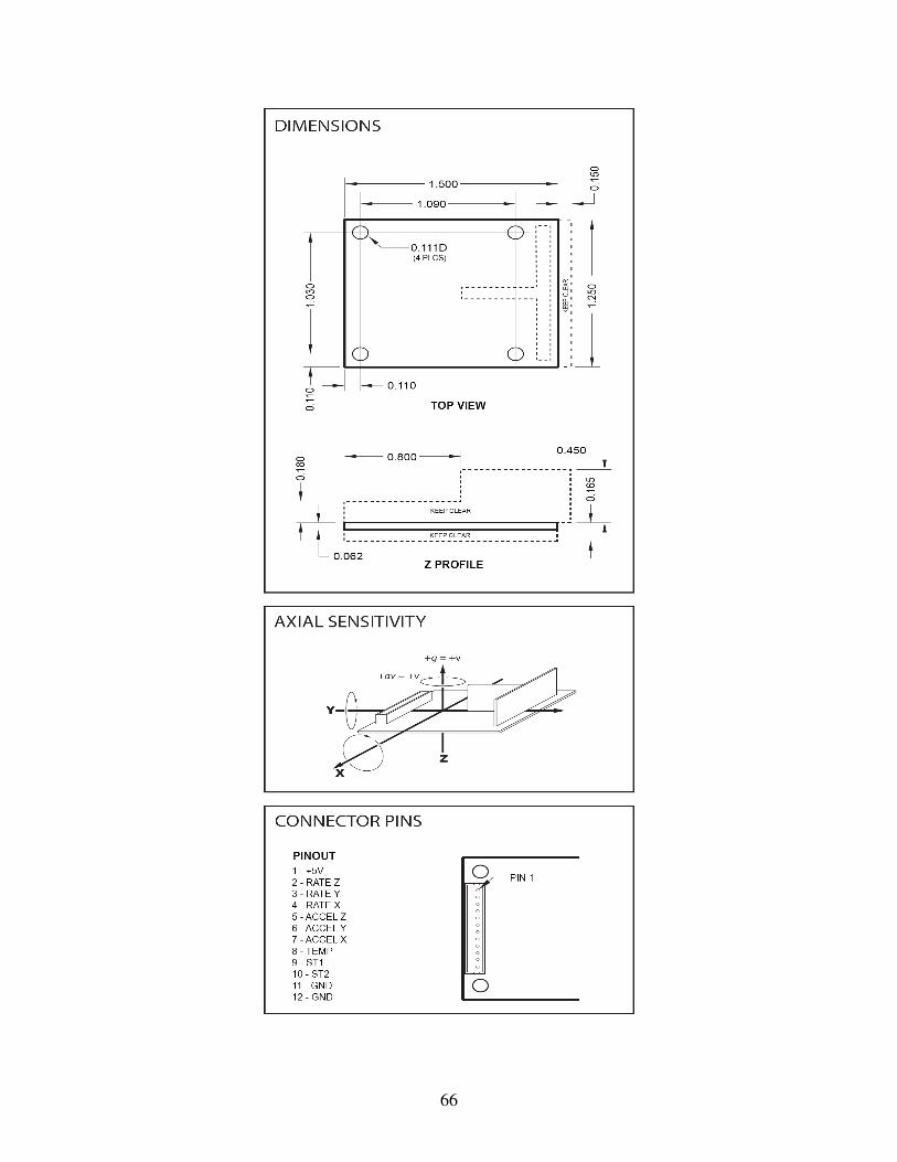
66

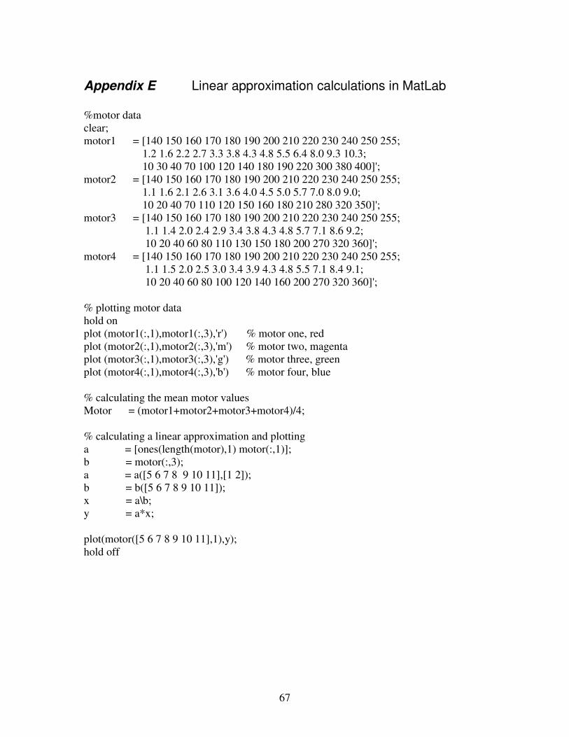
67

Appendix E Linear approximation calculations in MatLab

%motor data clear; motor1 = [140 150 160 170 180 190 200 210 220 230 240 250 255; 1.2 1.6 2.2 2.7 3.3 3.8 4.3 4.8 5.5 6.4 8.0 9.3 10.3; 10 30 40 70 100 120 140 180 190 220 300 380 400]'; motor2 = [140 150 160 170 180 190 200 210 220 230 240 250 255; 1.1 1.6 2.1 2.6 3.1 3.6 4.0 4.5 5.0 5.7 7.0 8.0 9.0; 10 20 40 70 110 120 150 160 180 210 280 320 350]'; motor3 = [140 150 160 170 180 190 200 210 220 230 240 250 255; 1.1 1.4 2.0 2.4 2.9 3.4 3.8 4.3 4.8 5.7 7.1 8.6 9.2; 10 20 40 60 80 110 130 150 180 200 270 320 360]'; motor4 = [140 150 160 170 180 190 200 210 220 230 240 250 255; 1.1 1.5 2.0 2.5 3.0 3.4 3.9 4.3 4.8 5.5 7.1 8.4 9.1; 10 20 40 60 80 100 120 140 160 200 270 320 360]'; % plotting motor data hold on plot (motor1(:,1),motor1(:,3),'r') % motor one, red plot (motor2(:,1),motor2(:,3),'m') % motor two, magenta plot (motor3(:,1),motor3(:,3),'g') % motor three, green plot (motor4(:,1),motor4(:,3),'b') % motor four, blue % calculating the mean motor values Motor = (motor1+motor2+motor3+motor4)/4; % calculating a linear approximation and plotting a = [ones(length(motor),1) motor(:,1)]; b = motor(:,3); a = a([5 6 7 8 9 10 11],[1 2]); b = b([5 6 7 8 9 10 11]); x = a\b; y = a*x; plot(motor([5 6 7 8 9 10 11],1),y); hold off

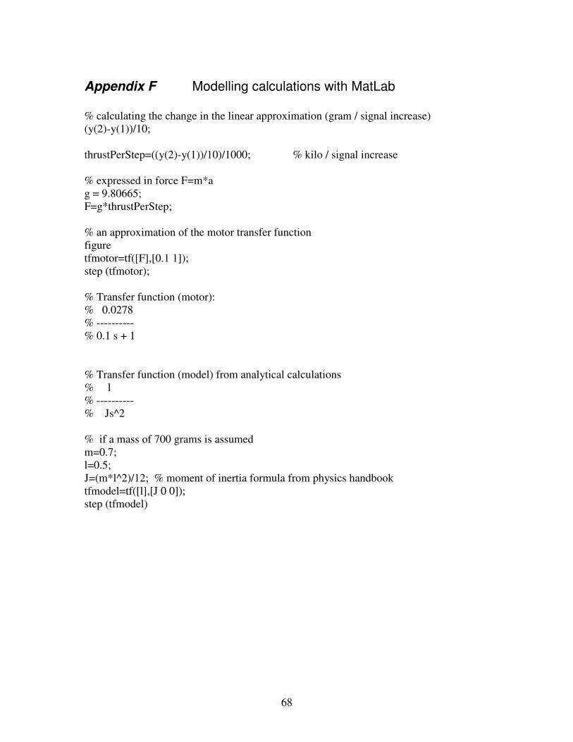
68

Appendix F Modelling calculations with MatLab

% calculating the change in the linear approximation (gram / signal increase) (y(2)-y(1))/10; thrustPerStep=((y(2)-y(1))/10)/1000; % kilo / signal increase % expressed in force F=m*a g = 9.80665; F=g*thrustPerStep; % an approximation of the motor transfer function figure tfmotor=tf([F],[0.1 1]); step (tfmotor); % Transfer function (motor): % 0.0278 % ---------- % 0.1 s + 1 % Transfer function (model) from analytical calculations % l % ---------- % Js^2 % if a mass of 700 grams is assumed m=0.7; l=0.5; J=(m*l^2)/12; % moment of inertia formula from physics handbook tfmodel=tf([l],[J 0 0]); step (tfmodel)

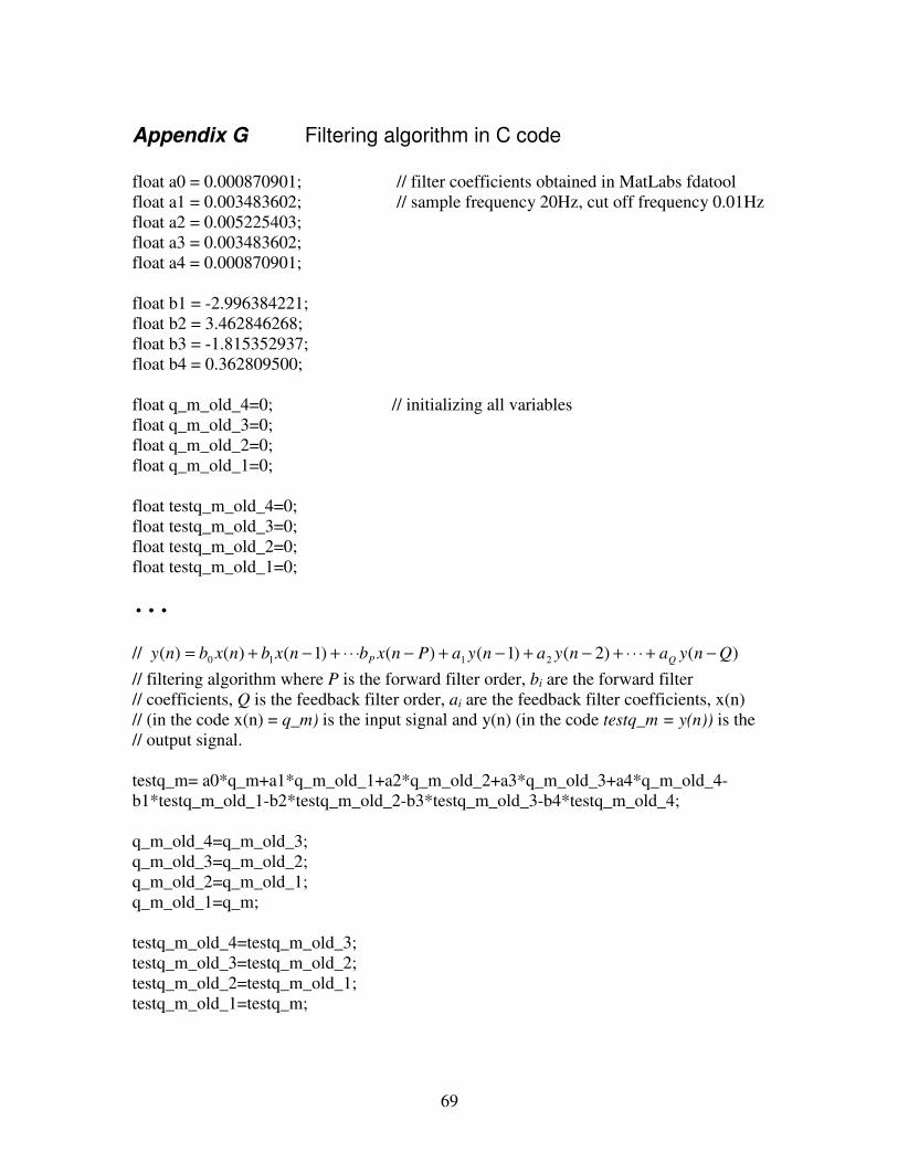
69

Appendix G Filtering algorithm in C code

float a0 = 0.000870901; // filter coefficients obtained in MatLabs fdatool float a1 = 0.003483602; // sample frequency 20Hz, cut off frequency 0.01Hz float a2 = 0.005225403; float a3 = 0.003483602; float a4 = 0.000870901; float b1 = -2.996384221; float b2 = 3.462846268; float b3 = -1.815352937; float b4 = 0.362809500; float q_m_old_4=0; // initializing all variables float q_m_old_3=0; float q_m_old_2=0; float q_m_old_1=0; float testq_m_old_4=0; float testq_m_old_3=0; float testq_m_old_2=0; float testq_m_old_1=0;

…

// )()2()1()()1()()( 2110 QnyanyanyaPnxbnxbnxbny QP −+⋅⋅⋅+−+−+−⋅⋅⋅+−+=

// filtering algorithm where P is the forward filter order, bi are the forward filter // coefficients, Q is the feedback filter order, ai are the feedback filter coefficients, x(n) // (in the code x(n) = q_m) is the input signal and y(n) (in the code testq_m = y(n)) is the // output signal. testq_m= a0*q_m+a1*q_m_old_1+a2*q_m_old_2+a3*q_m_old_3+a4*q_m_old_4-b1*testq_m_old_1-b2*testq_m_old_2-b3*testq_m_old_3-b4*testq_m_old_4; q_m_old_4=q_m_old_3; q_m_old_3=q_m_old_2; q_m_old_2=q_m_old_1; q_m_old_1=q_m; testq_m_old_4=testq_m_old_3; testq_m_old_3=testq_m_old_2; testq_m_old_2=testq_m_old_1; testq_m_old_1=testq_m;

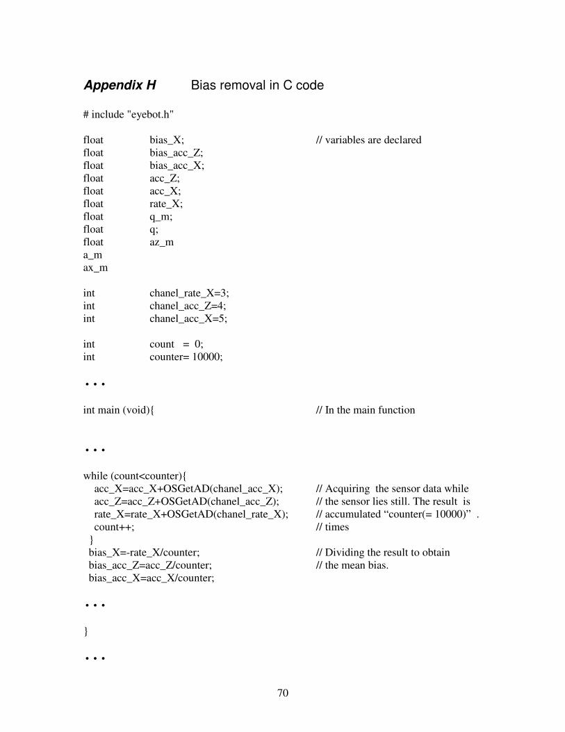
70

Appendix H Bias removal in C code

# include "eyebot.h" float bias_X; // variables are declared float bias_acc_Z; float bias_acc_X; float acc_Z; float acc_X; float rate_X; float q_m; float q; float az_m a_m ax_m int chanel_rate_X=3; int chanel_acc_Z=4; int chanel_acc_X=5; int count = 0; int counter= 10000;

…

int main (void) // In the main function

…

while (count<counter) acc_X=acc_X+OSGetAD(chanel_acc_X); // Acquiring the sensor data while acc_Z=acc_Z+OSGetAD(chanel_acc_Z); // the sensor lies still. The result is rate_X=rate_X+OSGetAD(chanel_rate_X); // accumulated “counter(= 10000)” . count++; // times bias_X=-rate_X/counter; // Dividing the result to obtain bias_acc_Z=acc_Z/counter; // the mean bias. bias_acc_X=acc_X/counter;

…

…

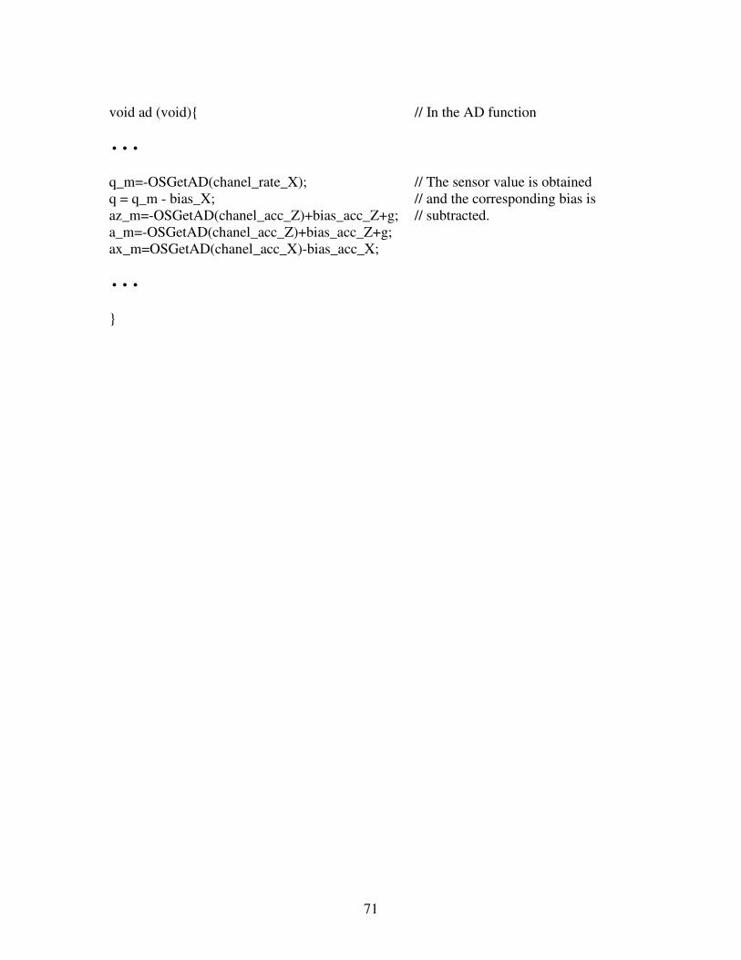
71

void ad (void) // In the AD function

…

q_m=-OSGetAD(chanel_rate_X); // The sensor value is obtained q = q_m - bias_X; // and the corresponding bias is az_m=-OSGetAD(chanel_acc_Z)+bias_acc_Z+g; // subtracted. a_m=-OSGetAD(chanel_acc_Z)+bias_acc_Z+g; ax_m=OSGetAD(chanel_acc_X)-bias_acc_X;

…

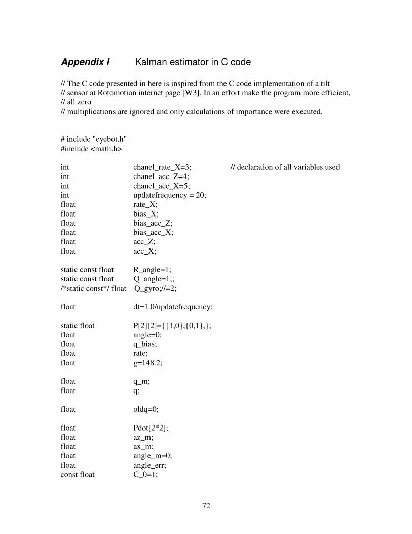
72

Appendix I Kalman estimator in C code

// The C code presented in here is inspired from the C code implementation of a tilt // sensor at Rotomotion internet page [W3]. In an effort make the program more efficient, // all zero // multiplications are ignored and only calculations of importance were executed. # include "eyebot.h" #include <math.h> int chanel_rate_X=3; // declaration of all variables used int chanel_acc_Z=4; int chanel_acc_X=5; int updatefrequency = 20; float rate_X; float bias_X; float bias_acc_Z; float bias_acc_X; float acc_Z; float acc_X; static const float R_angle=1; static const float Q_angle=1;; /*static const*/ float Q_gyro;//=2; float dt=1.0/updatefrequency; static float P[2][2]=1,0,0,1,; float angle=0; float q_bias; float rate; float g=148.2; float q_m; float q; float oldq=0; float Pdot[2*2]; float az_m; float ax_m; float angle_m=0; float angle_err; const float C_0=1;

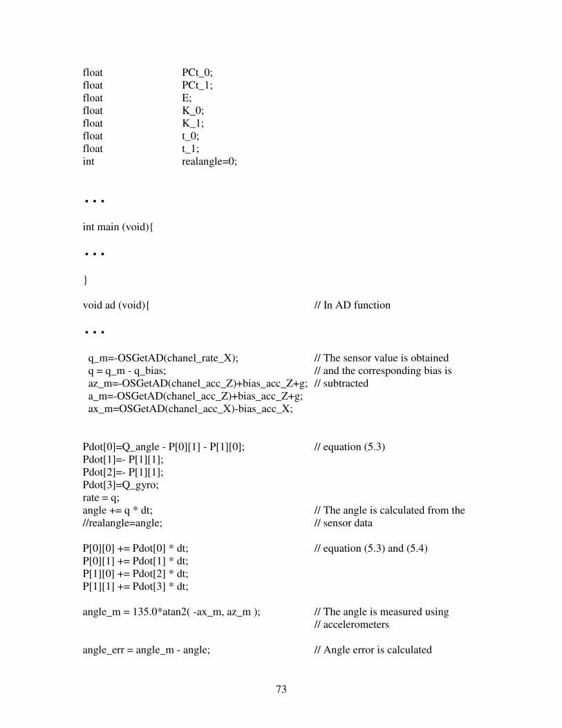
73

float PCt_0; float PCt_1; float E; float K_0; float K_1; float t_0; float t_1; int realangle=0;

…

int main (void)

…

void ad (void) // In AD function

…

q_m=-OSGetAD(chanel_rate_X); // The sensor value is obtained q = q_m - q_bias; // and the corresponding bias is az_m=-OSGetAD(chanel_acc_Z)+bias_acc_Z+g; // subtracted a_m=-OSGetAD(chanel_acc_Z)+bias_acc_Z+g; ax_m=OSGetAD(chanel_acc_X)-bias_acc_X; Pdot[0]=Q_angle - P[0][1] - P[1][0]; // equation (5.3) Pdot[1]=- P[1][1]; Pdot[2]=- P[1][1]; Pdot[3]=Q_gyro; rate = q; angle += q * dt; // The angle is calculated from the //realangle=angle; // sensor data P[0][0] += Pdot[0] * dt; // equation (5.3) and (5.4) P[0][1] += Pdot[1] * dt; P[1][0] += Pdot[2] * dt; P[1][1] += Pdot[3] * dt; angle_m = 135.0*atan2( -ax_m, az_m ); // The angle is measured using

// accelerometers

angle_err = angle_m - angle; // Angle error is calculated

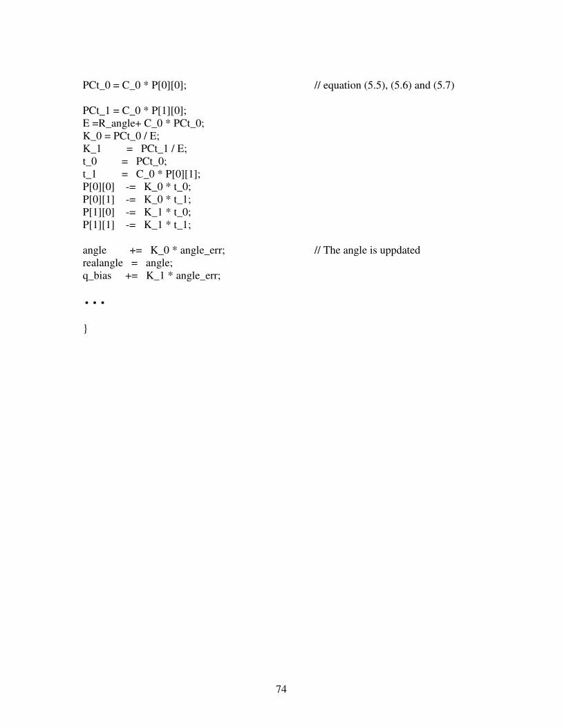
74

PCt_0 = C_0 * P[0][0]; // equation (5.5), (5.6) and (5.7) PCt_1 = C_0 * P[1][0]; E =R_angle+ C_0 * PCt_0; K_0 = PCt_0 / E; K_1 = PCt_1 / E; t_0 = PCt_0; t_1 = C_0 * P[0][1]; P[0][0] -= K_0 * t_0; P[0][1] -= K_0 * t_1; P[1][0] -= K_1 * t_0; P[1][1] -= K_1 * t_1; angle += K_0 * angle_err; // The angle is uppdated realangle = angle; q_bias += K_1 * angle_err;

…

75

Appendix J Anti alias filter calculations

The figure above shows the schematics of the second order Butterworth filter used as anti alias filter. In a low pass implementation G1 and G3 are resistors (R1 and R3) and G2 and G4 are capacitors (C2 and C4). The transfer function of the system above is

3141442

2

31

)()( GGGGsGGGs

GG

+++ (J.1)

Since the cut off frequency is decided by the relationship between the resistors and the

capacitors and it is known that 31 GG = in a Butterworth filter, it is advantageous to

simplify calculations by setting the resistors equal to one. This gives the following simplified transfer function

12)(

1

442

2 ++ GGGs (J.2)

It is known that a second order Butterworth has poles in

2

1

2

1js ±−= (J.3)

which corresponds to the following pole equation

12

22 ++ ss . (J.4)

Putting the two pole equations (J.2) and (J.4) together in an equation system gives that

G1

G2

G3

G4

+

_

OPA1014

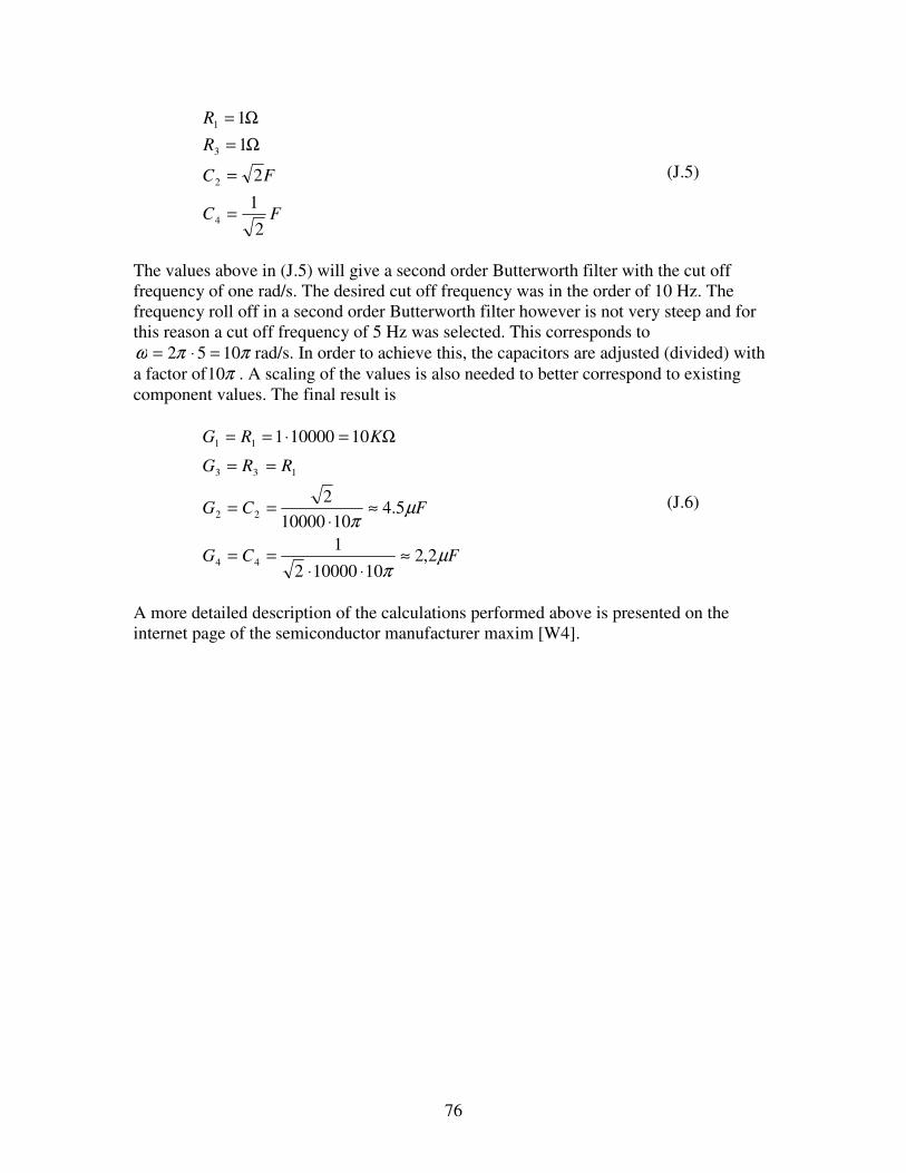
76

FC

FC

R

R

2

1

2

1

1

4

2

3

1

=

=

Ω=

Ω=

(J.5)

The values above in (J.5) will give a second order Butterworth filter with the cut off frequency of one rad/s. The desired cut off frequency was in the order of 10 Hz. The frequency roll off in a second order Butterworth filter however is not very steep and for this reason a cut off frequency of 5 Hz was selected. This corresponds to

ππω 1052 =⋅= rad/s. In order to achieve this, the capacitors are adjusted (divided) with

a factor of π10 . A scaling of the values is also needed to better correspond to existing component values. The final result is

FCG

FCG

RRG

KRG

µπ

µπ

2,210100002

1

5.41010000

2

10100001

44

22

133

11

≈⋅⋅

==

≈⋅

==

==

Ω=⋅==

(J.6)

A more detailed description of the calculations performed above is presented on the internet page of the semiconductor manufacturer maxim [W4].

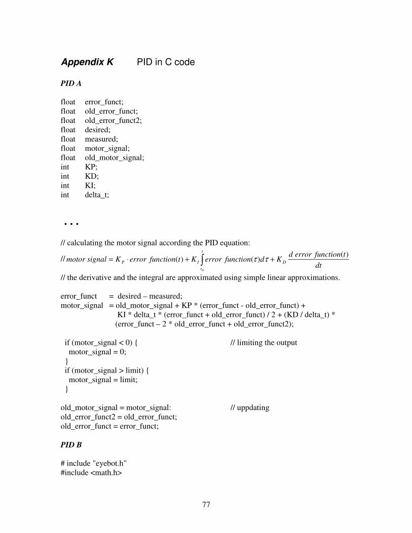
77

Appendix K PID in C code

PID A

float error_funct; float old_error_funct; float old_error_funct2; float desired; float measured; float motor_signal; float old_motor_signal; int KP; int KD; int KI; int delta_t;

… // calculating the motor signal according the PID equation:

//dt

tfunctionerrordKdfunctionerrorKtfunctionerrorKsignalmotor D

t

t

IP

)( )( )(

0

++⋅= ∫ ττ

// the derivative and the integral are approximated using simple linear approximations. error_funct = desired – measured; motor_signal = old_motor_signal + KP * (error_funct - old_error_funct) +

KI * delta_t * (error_funct + old_error_funct) / 2 + (KD / delta_t) * (error_funct – 2 * old_error_funct + old_error_funct2);

if (motor_signal < 0) // limiting the output motor_signal = 0; if (motor_signal > limit) motor_signal = limit; old_motor_signal = motor_signal: // uppdating old_error_funct2 = old_error_funct; old_error_funct = error_funct;

PID B

# include "eyebot.h" #include <math.h>

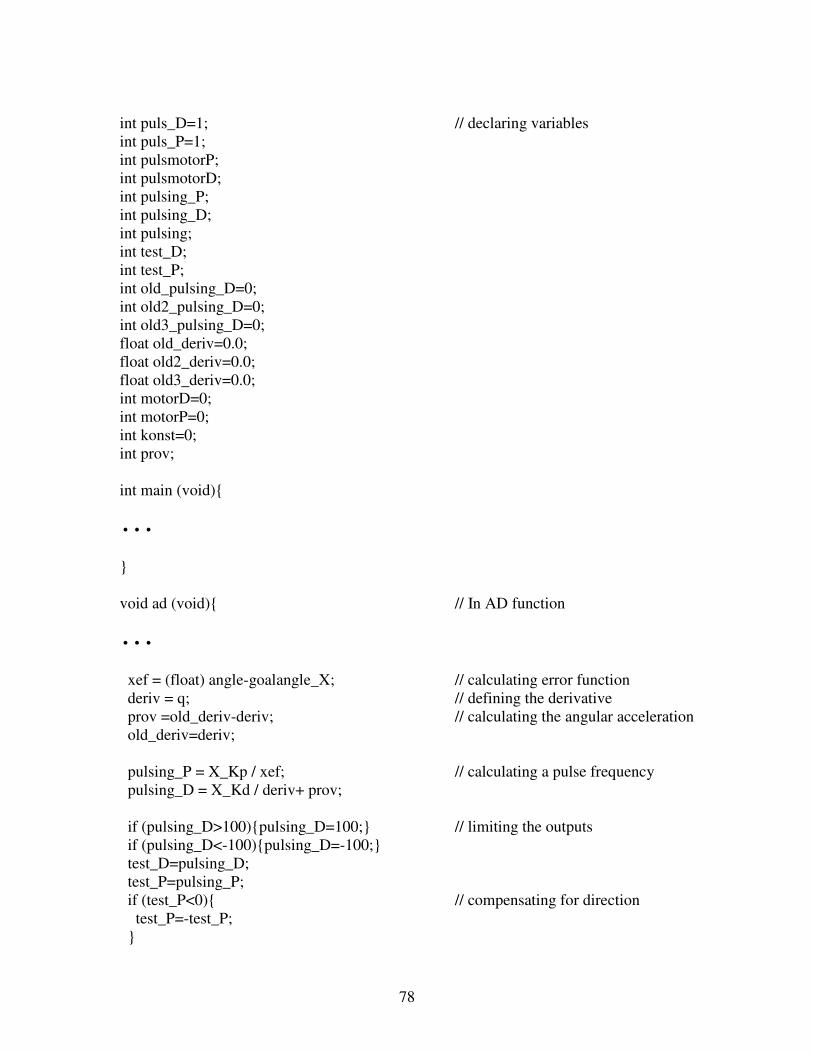
78

int puls_D=1; // declaring variables int puls_P=1; int pulsmotorP; int pulsmotorD; int pulsing_P; int pulsing_D; int pulsing; int test_D; int test_P; int old_pulsing_D=0; int old2_pulsing_D=0; int old3_pulsing_D=0; float old_deriv=0.0; float old2_deriv=0.0; float old3_deriv=0.0; int motorD=0; int motorP=0; int konst=0; int prov; int main (void)

…

void ad (void) // In AD function

…

xef = (float) angle-goalangle_X; // calculating error function deriv = q; // defining the derivative prov =old_deriv-deriv; // calculating the angular acceleration old_deriv=deriv; pulsing_P = X_Kp / xef; // calculating a pulse frequency pulsing_D = X_Kd / deriv+ prov; if (pulsing_D>100)pulsing_D=100; // limiting the outputs if (pulsing_D<-100)pulsing_D=-100; test_D=pulsing_D; test_P=pulsing_P; if (test_P<0) // compensating for direction test_P=-test_P;

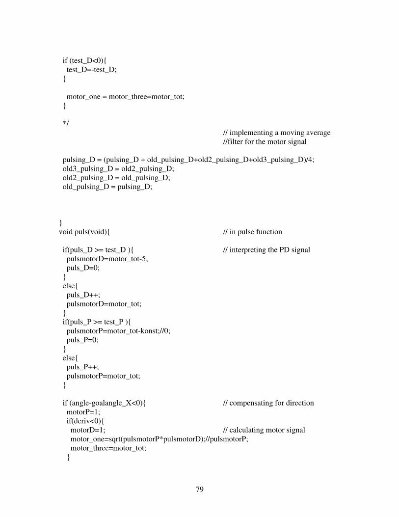
79

if (test_D<0) test_D=-test_D; motor_one = motor_three=motor_tot; */

// implementing a moving average //filter for the motor signal

pulsing_D = (pulsing_D + old_pulsing_D+old2_pulsing_D+old3_pulsing_D)/4; old3_pulsing_D = old2_pulsing_D; old2_pulsing_D = old_pulsing_D; old_pulsing_D = pulsing_D; void puls(void) // in pulse function if(puls_D >= test_D ) // interpreting the PD signal pulsmotorD=motor_tot-5; puls_D=0; else puls_D++; pulsmotorD=motor_tot; if(puls_P >= test_P ) pulsmotorP=motor_tot-konst;//0; puls_P=0; else puls_P++; pulsmotorP=motor_tot; if (angle-goalangle_X<0) // compensating for direction motorP=1; if(deriv<0) motorD=1; // calculating motor signal motor_one=sqrt(pulsmotorP*pulsmotorD);//pulsmotorP; motor_three=motor_tot;

80

else if (deriv>0) motorD=3; motor_three=pulsmotorD; motor_one=pulsmotorP; else if (angle-goalangle_X>0) motorP=3; if (deriv<0) motorD=1; motor_one=pulsmotorD; motor_three=pulsmotorP; else if (deriv>0) motorD=3; motor_three=sqrt(pulsmotorP*pulsmotorD);//pulsmotorP; motor_one=motor_tot; SERVOSet (servo2,motor_one); // setting motor speed SERVOSet (servo5,motor_three);

TRITA-CSC-E 2008:027 ISRN-KTH/CSC/E--08/027--SE

ISSN-1653-5715

www.kth.se