Controllability of simple mechanical control systemsandrew/talks/pdf/1998c.pdf · Slide0 Controllability of simple mechanical control systems Andrew D. Lewis∗ 27/08/1998 ∗Collaborators:

Slide 0

Controllability of simple mechanical control

systems

Andrew D. Lewis∗

27/08/1998

∗Collaborators: F. Bullo and R. Murray

Notes for Slide 0

The work presented in this talk was initiated by some work which went into my PhD disserta-tion [Lewis 1995], and has been ongoing, to some extent, ever since. The initial aim of the workwas to address some of the basic nonlinear control questions in the specific context of mechan-

ical systems. Although there is some fairly general work in the Hamiltonian control framework(see [Nijmeijer and van der Schaft 1990, Chapter 12]), existing work in the Lagrangian frameworkwas ad hoc and example based. Examples commonly studied were robotic systems and satellitecontrol. Since these systems are “simple” (i.e., their Lagrangians are kinetic minus potentialenergy), as are many mechanical control systems which arise in applications, it seems reasonableto focus on this class of systems.

Andrew D. Lewis University of Warwick

Slide 1

1. What are we after?

• Consider a linear control system:

x(t) = Ax(t) +Bu(t) (1)

x ∈ Rn, u ∈ R

m, A ∈ L(Rn;Rn), and B ∈ L(Rm;Rn).

• Starting at x = 0, where can we go?

• Linear system =⇒ basic questions have answers.

• R(0) = spanR([B|AB| . . . |An−1B]) (computable).

• R(0) is the smallest A-invariant subspace containing image(B)

(“geometric” meaning).

• We want to do something similar for a class of mechanical systems.

Notes for Slide 1

Since the idea of control may not be all that familiar, let me make sure we understand what thelinear system (1) represents. One should think of t 7→ u(t) as being a specified signal, i.e., afunction on the time interval [0, T ] (say). The job of a control theoretician is to design thesignal to make the “state” t 7→ x(t) do what we want. What this is may vary, depending on thesituation at hand. For example, one may want to steer from an initial state xi to a final statexf , perhaps in an optimal way. Or, one may wish to design u : Rn → R

m so that some state,perhaps x = 0, is stable for the dynamical system x = Ax + Bu(x). This latter is called state

feedback (often one asks that u be linear). One could also design u to be a function of both xand t. I think we get the idea. . .

One of the basic control questions is controllability, which comes in many guises, some ofwhich we shall take some care with later. For now, let us just say we are asking for “reachable”points. In particular, R(0) denotes the set of points reachable from 0 ∈ R

n. For linear systemswe provide two equivalent answers which have different flavours. The first answer is nice becausewith it one can compute the set of reachable points. However, it presents a somewhat “non-obvious appearance.” The second answer is nice because it sounds “believable,” and it givesone some insight into how the components of the control system (here the matrices A and B)interact to provide the set of reachable points.


Slide 2

2. Simple mechanical control systems

• Our systems are characterised by:

◦ an n-dimensional configuration manifold Q;

◦ a Riemannian metric g on Q (kinetic energy);

◦ a potential energy function V on Q;

◦ linearly independent one-forms F 1, . . . , Fm on Q (input forces).

• To make life easier, let us suppose V = 0 unless otherwise stated.

• We shall always consider initial conditions with zero velocity, and we

are interested in the reachable configurations.

• Such systems are not amenable to linearisation-based methods.

Notes for Slide 2

Some of our results require problem data to be analytic. So, to be safe, let us suppose this tobe the case. That is, suppose Q, g, V , and {F 1, . . . , Fm} to be analytic.

Of course, the Lagrangian we use given the above problem data is L(vq) =12g(vq, vq)−V (q)

where vq ∈ TqQ.Some of the results which we state have analogues when V 6= 0, but they are somewhat

awkward to state. Therefore we shall simply say when these analogous results exist withoutbeing too specific about them. Besides, the results when V 6= 0 are interesting and beautiful(particularly the latter, in my opinion) in their own right.

When we say these systems are not amenable to linearisation-based methods, we meanthat their linearisations at zero velocity are not controllable, and that they are not feedbacklinearisable. This makes simple mechanical control systems a non-trivial class of nonlinear controlsystems, especially from the point of view of control design.


Slide 3

3. Examples of simple mechanical control systems

• Robotic leg:

• Inputs are (1) an internal torque moving the leg relative to the body

and (2) a force extending the leg, i.e., F 1 = dθ − dψ and F 2 = dr.

Notes for Slide 3

The robotic leg has been studied as a nonholonomic system (i.e., one of the form q(t) =uaXa(q(t)) for vector fields X1, . . . , Xm on Q) by Li, Montgomery, and Raibert [1989] and Mur-ray and Sastry [1993]. Such a treatment differs somewhat from ours, but the two approachesare ultimately equivalent [Lewis 1999].

Interestingly, if one asks for the states (i.e., configurations and velocities) reachable fromconfigurations with zero initial velocity, one finds that not all states are reachable. This is aconsequence of the fact that angular momentum is conserved, even with inputs. Thus if onestarts with zero momentum, the momentum will remain zero (this is what enables one to treatthe system as nonholonomic). Nevertheless, all configurations are accessible. This suggests thatthe question of controllability is different depending on whether one is interested in configurationsor states. We have formally declared our interest in reachable configurations.

Considering the system with just one of the two possible input forces is also interesting. Inthe case where we are just allowed to use F 2, the possible motions are quite simple; one canonly move the ball on the leg back and forth. With just the force F 1 available, things are a bitmore complicated. But, for example, one can still say that no matter how you apply the force,the ball with never move “inwards.”


Slide 4

• The planar rigid body:

• Use coordinates (x, y, θ).

• Inputs are (1) force pointing towards centre of mass,

F 1 = cos θdx+ sin θdy, (2) force orthogonal to line to centre of

mass, F 2 = − sin θdx+ cos θdy − hdθ, and (3) torque at centre of

mass F 3 = dθ.

Notes for Slide 4

The planar rigid body, although seemingly quite simple, is actually somewhat interesting. Ofcourse, if one uses all three inputs, the system is fully actuated, and so boring for what we aredoing (investigating reachable configurations, that is). But if one takes various combinations ofone or two inputs, one gets a pretty nice sampling of what can happen for these systems. Forexample, all possible combinations of two inputs allow one to reach all configurations. UsingF 1 or F 3 alone give simple, one-dimensional reachable sets (similar to using F 2 for the roboticleg). Remember we are always starting with zero initial velocity! However, if one is allowed toonly use F 2, then it is not quite clear what to expect, at least just on the basis of intuition.


Slide 5

4. Recap of our objectives

• Note: All problem data is on Q =⇒ expect answers to be

describable using data on Q.

• We expect computations to simplify because of zero initial velocity

assumption, and because we are interested in reachable

configurations.

• We want a “computable” description of the reachable

configurations.

• How do the input one-forms F 1, . . . , Fm interact with the unforced

mechanics of the system as described by the kinetic energy

Riemannian metric?

Notes for Slide 5

It turns out that our simplifying assumptions, i.e., zero initial velocity and restriction of ourinterest to configurations, makes our task much simpler. In fact, the computations withoutthese assumptions have been attempted, but have yet to yield coherent answers.

In some sense, we wish to emulate the results we gave for linear systems at the beginningof the talk. And we shall in fact be able to do exactly this, inasmuch as it is possible. Withoutknowing the answer, it is worth thinking about the question of how the inputs interact withthe Riemannian metric. That is, what is the analogue of “the smallest A-invariant subspacecontaining image(B)” for simple mechanical control systems?


Slide 6

5. The formal setting up of the problem

• We letg

∇ denote the Levi-Civita affine connection for the

Riemannian metric g.

• The equations of motion are theng

∇c′(t)c′(t) = ua(t)Ya(c(t)) where

Ya = (F a)♯, a = 1, . . . ,m.

• There is nothing to be gained by using a Levi-Civita connection, or

by assuming that the vector fields come from one-forms. . . So we

study the control system

∇c′(t)c′(t) = ua(t)Ya(c(t))

(

+Y0(c(t)))

(CS)

with ∇ a general affine connection on Q, and Y1, . . . , Ym linearly

independent vector fields on Q.

Notes for Slide 6

Let us briefly recall how the Levi-Civita affine connection comes up in the problem. If we letL(q, v) = gij q

iqj , then the Euler-Lagrange equations are

gij qj +

(

∂gij∂qk

−1

2

∂gjk∂qi

)

qj qk = uaFai , i = 1, . . . , n.

Now multiply this by gli and take the symmetric part of the coefficient of qj qk to get ql +

Γljk q

j qk = uaY la , l = 1, . . . , n, where Γi

jk = 12g

il(

∂glj∂qk

+ ∂glk∂qj

−∂gjk∂ql

)

, i, j, k = 1, . . . , n, are

exactly the Christoffel symbols for the Levi-Civita connection.Here ♯ : T ∗Q→ TQ is the musical isomorphism associated with the Riemannian metric g.At this point, perhaps the generalisation to an arbitrary affine connection seems like a sense-

less abstraction. However, as we shall see, this abstraction allows us to include, for “free,”another large class of mechanical control systems.

The “optional” term Y0 in (CS) indicates how potential energy may be added. In this caseY0 = − gradV . However, one looses nothing by considering a general vector field instead ofa gradient. But I want to emphasise that one should always take Y0 = 0 below, unless it isotherwise stated.


Slide 7

• A solution to (CS) is a pair (c, u) satisfying (CS) where

c : [0, T ] → Q is a curve and u : [0, T ] → Rm is (say) bounded and

measurable.

• Let U be a neighbourhood of q0 ∈ Q and denote by RUQ(q0, T )

those points in Q for which there exists a solution (c, u) with the

properties

1. c(t) ∈ U for t ∈ [0, T ],

2. c′(0) = 0q, and

3. c(T ) ∈ TqQ.

• Also RUQ(q0,≤ T ) =

⋃

0≤t≤T RUQ(q0, t).

Notes for Slide 7

The following picture

gives an idea of what is meant by RUQ(q0, T ). It is the precise description of reachable sets as

we shall need them. Note that we do not ask for the final velocity to be zero.As you can see, we are only interested in points which can be reached without taking “large

excursions.” Control problems which are local in this way have the advantage that they can becharacterised (at least for analytic systems) by Lie brackets. We do not address global issues,but they generally fall into two classes: (1) those of a topological nature (e.g., compactnessin [San Martin and Crouch 1984]) and (2) those exploiting the unforced dynamics (e.g., Poissonstable systems in [Manikonda and Krishnaprasad 1997]).


Slide 8

• We want to “describe” RUQ(q,≤ T ).

• (CS) is locally configuration accessible (LCA) at q if there exists

T > 0 so that RUQ(q,≤ t) contains a non-empty open subset of Q

for each neighbourhood U of q and each t ∈ ]0, T ].

• (CS) is locally configuration controllable (LCC) at q if there exists

T > 0 so that RUQ(q,≤ t) contains a neighbourhood of q for each

neighbourhood U of q and each t ∈ ]0, T ].

Notes for Slide 8

The notions of local configuration accessibility (on the left in the picture below) and localconfiguration controllability (on the right in the picture below) are genuinely different.

Indeed, one need only look at the example of the robotic leg with the F 1 input. In this exampleone may show that the system is LCA, but is not LCC. To show the former is something wewill get to momentarily. The latter is clear for the reasons we have already mentioned: the ballcannot move “inward” no matter what kind of inputs you use.


Slide 9

6. Local configuration accessibility

• The accessibility problem is solved by looking at Lie brackets.

• Write (CS) in first order form: v = Z(v) + ua vlft(Ya(v)) where Z

is the geodesic spray for ∇.

• We evaluate all brackets at 0q—recall T0qTQ ≃ TqQ⊕ TqQ.

• We need the symmetric product: 〈X : Y 〉 = ∇XY +∇YX .

• Here are some sample brackets:

1. [Z, vlft(Ya)](0q) = (−Ya(q), 0);

2. [vlft(Ya), [Z, vlft(Yb)]](0q) = (0, 〈Ya : Yb〉(q));

3. [[Z, vlft(Ya)], [Z, vlft(Yb)]](0q) = ([Ya, Yb](q), 0).

Notes for Slide 9

Recall the vertical lift:

vlft(Y )(vq) =d

dt

∣

∣

∣

t=0(vq + tY (q)).

In coordinates, if Y = Y i ∂∂qi

, then vlft(Y ) = Y i ∂∂vi .

When we write T0qTQ = TqQ ⊕ TqQ, the first component we think of as being the “hori-zontal” bit which is tangent to the zero section in TQ, and we think of the second componentas being the “vertical” bit which is the tangent space to the fibre of πTQ : TQ→ Q.

To get an answer to the local configuration accessibility problem, we employ standard nonlin-ear control techniques involving Lie brackets. Doing so gives us our first look at the symmetricproduct. Our sample brackets suggest that perhaps the only things which appear in the bracketcomputations are symmetric products and Lie brackets of the input vector fields Y1, . . . , Ym.This is, in fact, the case, and the way they appear is also interesting as we shall see.


Slide 10

• Let Cver be the closure of span(Y1, . . . , Ym) under symmetric

product.

• Let Chor be the closure of Cver under Lie bracket.

• The closure of span(Z, vlft(Y1), . . . , vlft(Ym)) under Lie bracket,

when evaluated at 0q, is then the distribution

q 7→ Chor(q)⊕ Cver(q) ⊂ TqQ⊕ TqQ.

• Chor is integrable—let Λq be the maximal integral manifold through

q ∈ Q.

Theorem 1 RUQ(q,≤ T ) is contained in Λq, and R

UQ(q,≤ T )

contains a non-empty open subset of Λq. In particular, if

rank(Chor) = n then (CS) is LCA.

Notes for Slide 10

We tacitly assume Cver and Chor to be distributions (i.e., of constant rank) on Q. With ourunderlying analyticity assumption, this will be true on an open dense subset of Q. Proving thatthe involutive closure of span(Z, vlft(Y1), . . . , vlft(Ym)) is equal at 0q to Chor(q) ⊕ Cver(q) isa matter of computing brackets, samples of which are given on the previous slide, and seeingthe patterns to suggest an inductive proof. The brackets for these systems are very structured.For example, the brackets of input vector fields are identically zero. Many other brackets vanishidentically, and many more vanish when evaluated at 0q. For details on the bracket computations,including systems with potential energy, we refer to [Lewis and Murray 1997a]. With potentialenergy included, the computations get rather messy.


Slide 11

7. The geometry of the reachable configurations

• What is the geometric meaning of Cver and Chor?

• Recall: A submanifold M of Q is totally geodesic if every geodesic

with initial velocity tangent to M remains on M .

• Weaken to distributions: a distribution D on Q is geodesically

invariant if for every geodesic c : [0, T ] → Q, c′(0) ∈ Dc(0) implies

c′(t) ∈ Dc(t) for t ∈ ]0, T ].

Theorem 2 D is geodesically invariant iff it is closed under

symmetric product.

Notes for Slide 11

Theorem 1 gives a “computable” description of the reachable sets (in the sense that you cancompute Λq by solving some over-determined nonlinear pde’s). But it does not give the kindof insight that we had with the “smallest A-invariant subspace containing image(B).” It is thiswhich we now describe.

Note that Theorem 2 says that the symmetric product plays for geodesically invariant dis-tributions the same role the Lie bracket plays for integrable distributions. The result is provedby [Lewis 1998]. This result was key in providing the geometric description of the reachableconfigurations.


Slide 12

• An integrable distribution is geodesically generated if it is the

involutive closure of a geodesically invariant distribution.

• Clearly Cver is the smallest geodesically invariant distribution

containing span(Y1, . . . , Ym).

• Also, Chor is “geodesically generated” by span(Y1, . . . , Ym).

• Thus RUQ is contained in, and contains a non-empty open subset of,

the distribution geodesically generated by span(Y1, . . . , Ym).

Notes for Slide 12

To be geodesically generated basically means that one may reach all points on a leaf withgeodesics lying in some subdistribution.

The picture one should have in mind with the geometry of the reachable sets is a foliation ofQ by geodesically generated (immersed) submanifolds onto which the control system restricts ifthe initial velocity is zero.


The idea is that when you start with zero velocity you remain on leaves of the foliation definedby Chor. This decomposition is described by Lewis and Murray [1997b]. Note that for caseswhen the affine connection possesses no geodesically invariant distributions, the system (CS) isautomatically LCA. This is true, for example, of S2 with the affine connection associated withits round metric.

We should also mention that the pretty decomposition we have for systems with no potentialenergy does not exist at this point for systems with potential energy.


Slide 13

8. Local configuration controllability

• This is harder. . .

• Call a symmetric product in {Y1, . . . , Ym} bad if it contains an even

number of each of the input vector fields. Otherwise call it good.

The degree is the total number of vector fields.

• For example, 〈〈Ya : Yb〉 : 〈Ya : Yb〉〉 is bad and of degree 4, and

〈Ya : 〈Yb : Yb〉〉 is good and of degree 3.

Theorem 3 If each bad symmetric product at q is a linear

combination of good symmetric products of lower degree, then (CS)

is LCC at q.

Notes for Slide 13

This business of good and bad symmetric products comes from an adaptation of work of Hermes[1982] and Sussmann [1983, 1987]. Theorem 3 was proven in [Lewis and Murray 1997a]. Toproperly state the result, one should use free Lie and symmetric algebras.


Slide 14

• The single-input case can be solved completely:

Theorem 4 The system (CS) with m = 1 is LCC if and only if

dim(Q) = 1.

• The local controllability question for general single-input control

systems has not been answered =⇒ our systems are special?

=⇒

the controllability question may be solvable for arbitrary numbers of

inputs!

Notes for Slide 14

The single-input result we state here follows (with some modification) from a result of Sussmann[1983]. It is presented in [Lewis 1997]. Although it seems an innocuous enough result, it isactually quite important for the reasons stated: it suggests that perhaps the general problem oflocal configuration controllability for these systems is solvable. This would be quite interesting asthere are not many classes of systems for which this is the case, never mind that the mechanicalsystems we are looking at come up often in applications.

The result we state is not generally true for systems with potential energy. In particular,there are single-input systems with potential energy which are LCC at certain configurations.For example, the “crane,”

with the single input being a horizontal force applied to the base, is LCC about both verticalconfigurations of the arm.


Slide 15

9. Systems with nonholonomic constraints

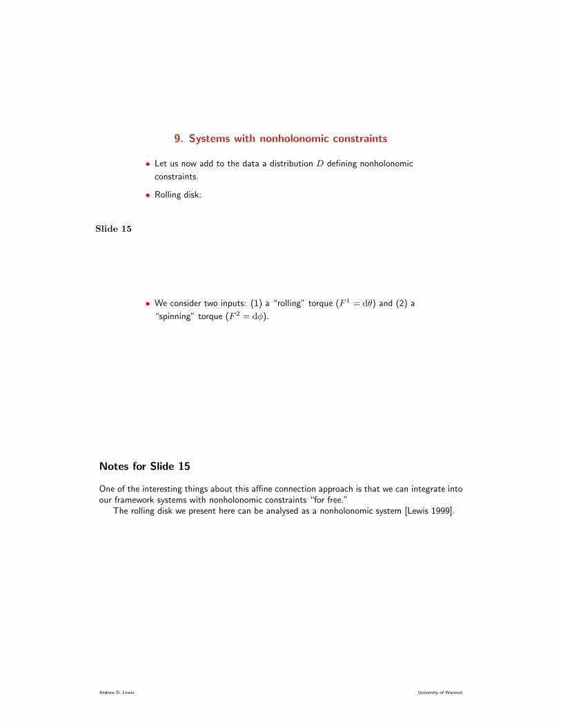
• Let us now add to the data a distribution D defining nonholonomic

constraints.

• Rolling disk:

• We consider two inputs: (1) a “rolling” torque (F 1 = dθ) and (2) a

“spinning” torque (F 2 = dφ).

Notes for Slide 15

One of the interesting things about this affine connection approach is that we can integrate intoour framework systems with nonholonomic constraints “for free.”

The rolling disk we present here can be analysed as a nonholonomic system [Lewis 1999].


Slide 16

• The control equations for a simple mechanical control system with

constraints are

g

∇c′(t)c′(t) = λ(t) + ua(t)Ya(c(t))

(

− gradV (c(t)))

c′(t) ∈ Dc(t)

where λ(t) ∈ D⊥c(t) are Lagrange multipliers.

• Let P : TQ→ TQ and P ′ : TQ→ TQ be orthogonal projections

onto D and D⊥, respectively

• Define an affine connectionD

∇ by

D

∇XY =g

∇XY + (g

∇XP′)(Y )

Notes for Slide 16

The idea of writing constrained equations for simple mechanical systems with an affine con-nection seems to date to Synge [1928]. It has been rediscovered many times since then. Forexample, Bloch and Crouch [1995] use a variant of what we do here to investigate integrabilityof nonholonomic systems.

The properties of the affine connectionD

∇ are discussed, along with other topics involvingaffine connections and distributions, in [Lewis 1998].


Slide 17

• The control equations are then equivalent to

D

∇c′(t)c′(t) = ua(t)P (Ya)(c(t))

(

−P (gradV )(c(t)))

which is of the form (CS).

• All the above analysis applies verbatim.

• Examples are somewhat unpleasant computationally. . .

Notes for Slide 17

The derivation of the constrained control equations in affine connection form is given by [Lewis2000]. In that paper, a sometimes useful computational simplification is also presented. I havewritten a Mathematica package to do some of these computations, but they are still prettyhorrific for non-trivial examples.


Slide 18

10. Examples (some revisited)

• Recall Y1 was internal torque and Y2 was extension force.

◦ Both inputs: LCA and LCC (satisfies sufficient condition).

◦ Y1 only: LCA but not LCC.

◦ Y2 only: not LCA.

Notes for Slide 18

In the three cases, Chor is generated by the following linearly independent vector fields:

1. Both inputs: {Y1, Y2, [Y1, Y2]};

2. Y1 only: {Y1, 〈Y1 : Y1〉, 〈Y1 : 〈Y1 : Y1〉〉};

3. Y2 only: {Y2}.

Of course, these generators are not unique.The sufficient condition we refer to here is the good/bad symmetric product result, Theo-

rem 3.Recall that with both inputs the system (we claimed) was not accessible in TQ as a conse-

quence of conservation of angular momentum.With the input Y2 only, the control system behaves very simply when given zero initial

velocity. The ball on the end of the leg just gets moved back and forth. This reflects thefoliation of Q by the maximal integral manifolds of Chor, which are evidently one-dimensionalin this case.

With the Y1 input, recall that the ball will always fly “outwards” no matter what one doeswith the input. Thus the system is not LCC. But apparently (since rank(Chor) = dim(Q)) onecan reach a non-empty open subset of Q. The behaviour exhibited in this case is typical of whatone can expect for single-input systems with no potential energy.


Slide 19

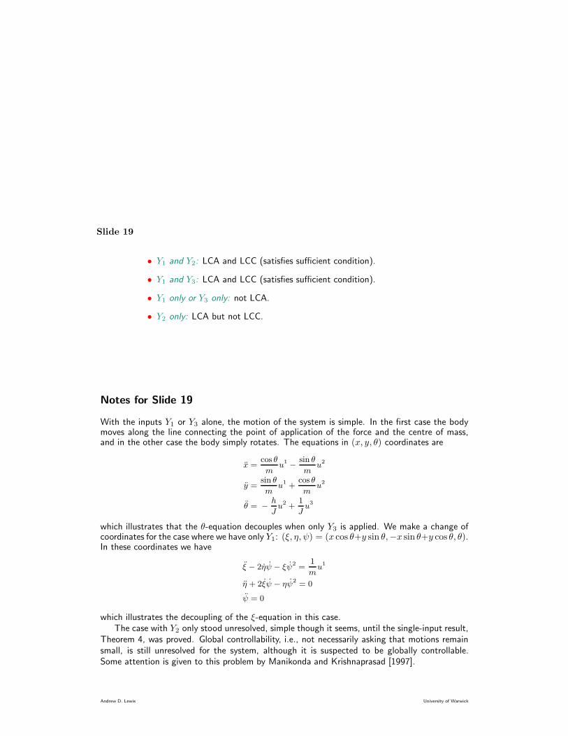
• Y1 and Y2: LCA and LCC (satisfies sufficient condition).

• Y1 and Y3: LCA and LCC (satisfies sufficient condition).

• Y1 only or Y3 only: not LCA.

• Y2 only: LCA but not LCC.

Notes for Slide 19

With the inputs Y1 or Y3 alone, the motion of the system is simple. In the first case the bodymoves along the line connecting the point of application of the force and the centre of mass,and in the other case the body simply rotates. The equations in (x, y, θ) coordinates are

x =cos θ

mu1−

sin θ

mu2

y =sin θ

mu1+

cos θ

mu2

θ = −

h

Ju2+

1

Ju3

which illustrates that the θ-equation decouples when only Y3 is applied. We make a change ofcoordinates for the case where we have only Y1: (ξ, η, ψ) = (x cos θ+y sin θ,−x sin θ+y cos θ, θ).In these coordinates we have

ξ − 2ηψ − ξψ2=

1

mu1

η + 2ξψ − ηψ2= 0

ψ = 0

which illustrates the decoupling of the ξ-equation in this case.The case with Y2 only stood unresolved, simple though it seems, until the single-input result,

Theorem 4, was proved. Global controllability, i.e., not necessarily asking that motions remainsmall, is still unresolved for the system, although it is suspected to be globally controllable.Some attention is given to this problem by Manikonda and Krishnaprasad [1997].


Slide 20

• Y2 and Y3: LCA and LCC (fails sufficient condition).

Notes for Slide 20

Chor has the following generators:

1. Y1 and Y2: {Y1, Y2, [Y1, Y2]};

2. Y1 and Y3: {Y1, Y3, [Y1, Y3]};

3. Y1 only or Y3 only: {Y1} or {Y3};

4. Y2 only: {Y2, 〈Y2 : Y2〉, 〈Y2 : 〈Y2 : Y2〉〉}.

5. Y2 and Y3: {Y2, Y3, [Y2, Y3]}.

The inputs we deal with in this slide do give a system which is LCC, but which fails ourgood/bad symmetric product test. However, a simple change of input, as illustrated in the figure,suggests that the system ought to be LCC. In fact, with these modified inputs, the system nowsatisfies the conditions of Theorem 3. A possible conjecture is that this is always possible. Thatis, perhaps (CS) is LCC if and only if there exists a basis of input vector fields which satisfy thehypotheses of Theorem 3. But this is speculation at this point. . .


Slide 21

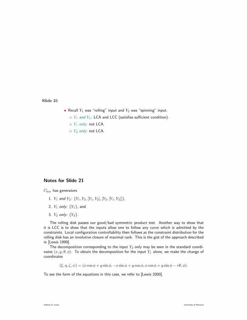
• Recall Y1 was “rolling” input and Y2 was “spinning” input.

◦ Y1 and Y2: LCA and LCC (satisfies sufficient condition).



Notes for Slide 21

Chor has generators

1. Y1 and Y2: {Y1, Y2, [Y1, Y2], [Y2, [Y1, Y2]]},

2. Y1 only: {Y1}, and

3. Y2 only: {Y2}.

The rolling disk passes our good/bad symmetric product test. Another way to show thatit is LCC is to show that the inputs allow one to follow any curve which is admitted by theconstraints. Local configuration controllability then follows as the constraint distribution for therolling disk has an involutive closure of maximal rank. This is the gist of the approach describedin [Lewis 1999].

The decomposition corresponding to the input Y2 only may be seen in the standard coordi-nates (x, y, θ, φ). To obtain the decomposition for the input Y1 alone, we make the change ofcoordinates

(ξ, η, ζ, ψ) = (x cosφ+ y sinφ,−x sinφ+ y cosφ, x cosφ+ y sinφ− rθ, φ).

To see the form of the equations in this case, we refer to [Lewis 2000].


Slide 22

• Take φ1 = φ2 = φ.

• Inputs are a synchronised torque to rotate the wheels (F 1 = dφ)

and a torque to rotate the “rider” (F 2 = dψ).

Notes for Slide 22

The snakeboard example we look at here was first investigated by Lewis, Ostrowski, Murray, andBurdick [1994]. As a nonholonomic system with symmetry it was further studied by Ostrowski[1995] and Bloch, Krishnaprasad, Marsden, and Murray [1996]. A different control treatment isgiven by Ostrowski and Burdick [1997].


Slide 23

• Caressing Mathematica gives:

◦ Y1 and Y2: LCA and LCC (satisfies sufficient condition).



Notes for Slide 23

Generators for Chor are

1. Y1 and Y2: {Y1, Y2, [Y1, Y2], [Y2, [Y1, Y2]], [Y2, [Y1, [Y2, [Y1, Y2]]]]},

2. Y1 only: {Y1}, and

3. Y2 only: {Y2}.

The computations for the snakeboard are somewhat unpleasant, and are given in detailby Lewis [2000]. Part of the reason the snakeboard equations are so awkward in affine connectionform is that the SE(2)-symmetry of the system is not taken into account as it is, for example,by Ostrowski and Burdick [1997]. It is probably interesting to see how symmetry figures intoour whole picture. The “fully symmetric” case where Q is a Lie group G is presented by [Bulloand Lewis 1996]. The case where Q→ Q/G is a principal bundle is next in line.

The motion with only the input Y1 is easy to describe: the wheels rotate and nothing elsehappens. With only Y2, the maximal integral manifolds of Chor are still one-dimensional, butare not so easy to describe (i.e., I don’t know what they look like).


Slide 24

• Single input: F = dθ − dψ.

• Probably LCA, but (definitely) not LCC.

Notes for Slide 24

I was not able to obtain an expression for generators for Chor for the roller racer. However, Chor

does not have full rank at the “standard” configuration (x = 0, y = 0, θ = 0, ψ = 0).The roller racer pictured here was studied by Krishnaprasad and Tsakiris [2001] as a system

with SE(2)-symmetry. Because we have not incorporated this into our framework, the rollerracer computations put even the snakeboard computations to shame. . . Nevertheless, Theo-rem 4 allows one to immediately say that local configuration controllability is impossible. Globalcontrollability is unresolved, but it seems likely that the roller racer is globally controllable.


Slide 25

11. Control design (F. Bullo)

• Up to now, consider case when Q = G and data is left-invariant.

• Use low amplitude, periodic inputs and averaging methods based on

controllability analysis.

◦ Steer the system from state (q1, 0) to (q2, 0) (with small final

error).

◦ Exponentially stabilise the system to (q0, 0) in a neighbourhood.

◦ Steer the system along a path connecting points q1, . . . , qN

(with small error terms).

Notes for Slide 25

Control design for these systems, especially in the absence of potential energy, is a bit challenging.This is a direct consequence of the system’s not being amenable to linearisation-based controldesign methods.

Averaging on Lie groups was used by Leonard and Krishnaprasad [1995] to study kinematicsystems, i.e., systems with no drift. It is possible to modify these methods to the systems weconsider, and this is done by Bullo, Leonard, and Lewis [2000], at least in some cases.

It should be mentioned that the exponential stabilisation of these systems is somewhat non-trivial. For example, they cannot be stabilised by continuous state feedback [Brockett 1983],and cannot be exponentially stabilised by smooth, time-varying feedback [M’Closkey and Murray1997]. The controllers defined by Bullo, Leonard, and Lewis [2000] are continuous and time-varying.


Slide 26

12. Stuff to do

• Figure out local accessibility at non-zero velocity.

• Get sharper controllability results.

• Refine understanding of how potential energy enters the picture.

• Control design for general systems.

• Optimal control.

• Punchline: The affine connection formalism can be useful.

Notes for Slide 26

Some preliminary bracket computations at non-zero initial velocity have been done. They arequite complicated. However, curvature and its derivatives appear, so one expects the infinitesimalholonomy algebra for ∇ to come into the picture. This is not altogether surprising.

As was suggested above, it might be possible to get very crisp controllability results for thesesystems, and this would be interesting. But almost nothing has been done in this area.

At this point, design methodology for controllers for the systems we have been talking aboutdo not really exist. The averaging methods as discussed above for Lie groups ought to be ableto be applied to general systems in some manner, but the details here have yet to be workedout. For some preliminary results see [Bullo 1999].

It would appear that these systems offer a very nice framework within which to study optimalcontrol. Nothing really has been done here, however.

If there were to be a point of this talk, it would be that the framework we provide here usingaffine connections to describe certain classes of mechanical control systems can be valuable,especially for obtaining general results. As another example of this, see [Lewis 1999] wherea concise recipe is given for deciding when a mechanical system is kinematic. I was forcedto consider such a condition by the propensity of some in the control community to equate

mechanical systems with “nonholonomic” systems. For example, I once saw someone talk aboutthe snakeboard as a nonholonomic system, which it most certainly is not! For work which is notmine (!) and which employs the affine connection, see [Rathinam and Murray 1998].


References

Bloch, A. M. and Crouch, P. E. [1995] Another view of nonholonomic mechanical control systems,in Proceedings of the 34th IEEE Conference on Decision and Control, pages 1066–1071,Institute of Electrical and Electronics Engineers, New Orleans, LA.

Bloch, A. M., Krishnaprasad, P. S., Marsden, J. E., and Murray, R. M. [1996] Nonholonomic

mechanical systems with symmetry, Archive for Rational Mechanics and Analysis, 136(1),21–99.

Brockett, R. W. [1983] Asymptotic stability and feedback stabilization, in Differential Geometric

Control Theory, R. W. Brockett, R. S. Millman, and H. J. Sussmann, editors, pages 181–191,number 27 in Progress in Mathematics, Birkhauser, Boston/Basel/Stuttgart, ISBN 3-7643-3091-0.

Bullo, F. [1999] A series describing the evolution of mechanical control systems, in Proceedings

of the IFAC World Congress, pages 479–485, IFAC, Beijing, China.

Bullo, F., Leonard, N. E., and Lewis, A. D. [2000] Controllability and motion algorithms for

underactuated Lagrangian systems on Lie groups, Institute of Electrical and Electronics Engi-neers. Transactions on Automatic Control, 45(8), 1437–1454.

Bullo, F. and Lewis, A. D. [1996] Configuration controllability of mechanical systems on Lie

groups, Proceedings of MTNS ’96.

Hermes, H. [1982] On local controllability, SIAM Journal on Control and Optimization, 20(2),211–220.

Krishnaprasad, P. S. and Tsakiris, D. P. [2001] Oscillations, SE(2)-snakes and motion control: a

study of the roller racer, Dynamics and Stability of Systems. An International Journal, 16(4),347–397.

Leonard, N. E. and Krishnaprasad, P. S. [1995]Motion control of drift-free, left-invariant systems

on Lie groups, Institute of Electrical and Electronics Engineers. Transactions on AutomaticControl, 40(9), 1539–1554.

Lewis, A. D. [1995] Aspects of Geometric Mechanics and Control of Mechanical Systems, Ph.D.thesis, California Institute of Technology, Pasadena, California, USA.URL: http://www.cds.caltech.edu/

— [1997] Local configuration controllability for a class of mechanical systems with a single input,in Proceedings of the 1997 European Control Conference, Brussels, Belgium.

— [1998] Affine connections and distributions with applications to nonholonomic mechanics,Reports on Mathematical Physics, 42(1/2), 135–164.

— [1999] When is a mechanical control system kinematic?, in Proceedings of the 38th IEEE

Conference on Decision and Control, pages 1162–1167, Institute of Electrical and ElectronicsEngineers, Phoenix, AZ.

— [2000] Simple mechanical control systems with constraints, Institute of Electrical and Elec-tronics Engineers. Transactions on Automatic Control, 45(8), 1420–1436.

Lewis, A. D. and Murray, R. M. [1997a] Controllability of simple mechanical control systems,SIAM Journal on Control and Optimization, 35(3), 766–790.

— [1997b] Decompositions of control systems on manifolds with an affine connection, Systems& Control Letters, 31(4), 199–205.


Lewis, A. D., Ostrowski, J. P., Murray, R. M., and Burdick, J. W. [1994] Nonholonomic mechan-

ics and locomotion: the Snakeboard example, in Proceedings of the 1994 IEEE International

Conference on Robotics and Automation, pages 2391–2400, Institute of Electrical and Elec-tronics Engineers, San Diego.

Li, Z., Montgomery, R., and Raibert, M. [1989] Dynamics and control of a legged robot in flight

phase, in Proceedings of the 1989 IEEE International Conference on Robotics and Automation,Institute of Electrical and Electronics Engineers, Scottsdale, AZ.

Manikonda, V. and Krishnaprasad, P. S. [1997] Controllability of Lie-Poisson reduced dynamics,in Proceedings of the 1997 American Control Conference, Albuquerque, NM.

M’Closkey, R. T. and Murray, R. M. [1997] Exponential stabilization of driftless nonlinear con-

trol systems using homogeneous feedback, Institute of Electrical and Electronics Engineers.Transactions on Automatic Control, 42(5), 614–628.

Murray, R. M. and Sastry, S. S. [1993] Nonholonomic motion planning: Steering using sinusoids,Institute of Electrical and Electronics Engineers. Transactions on Automatic Control, 38(5),700–716.

Nijmeijer, H. and van der Schaft, A. J. [1990] Nonlinear Dynamical Control Systems, Springer-Verlag, New York/Heidelberg/Berlin, ISBN 0-387-97234-X.

Ostrowski, J. P. [1995] The Mechanics and Control of Undulatory Robotic Locomotion, Ph.D.thesis, California Institute of Technology, Pasadena, California, USA.URL: http://www.cds.caltech.edu/

Ostrowski, J. P. and Burdick, J. W. [1997] Controllability tests for mechanical systems with

constraints and symmetries, Journal of Applied Mathematics and Computer Science, 7(2),101–127.

Rathinam, M. and Murray, R. M. [1998] Configuration flatness of Lagrangian systems underac-

tuated by one control, SIAM Journal on Control and Optimization, 36(1), 164–179.

San Martin, L. and Crouch, P. E. [1984] Controllability on principal fibre bundles with compact

structure group, Systems & Control Letters, 5(1), 35–40.

Sussmann, H. J. [1983] Lie brackets and local controllability: A sufficient condition for scalar-

input systems, SIAM Journal on Control and Optimization, 21(5), 686–713.

— [1987] A general theorem on local controllability, SIAM Journal on Control and Optimization,25(1), 158–194.

Synge, J. L. [1928] Geodesics in nonholonomic geometry, Mathematische Annalen, 99, 738–751.


Documents

Controllability of simple mechanical control systemsandrew/talks/pdf/1998c.pdf · Slide0 Controllability of simple mechanical control systems Andrew D. Lewis∗ 27/08/1998 ∗Collaborators: