Controlled estimation algorithms of disparity map using a

HAL Id: tel-03162847https://tel.archives-ouvertes.fr/tel-03162847

Submitted on 8 Mar 2021

HAL is a multi-disciplinary open accessarchive for the deposit and dissemination of sci-entific research documents, whether they are pub-lished or not. The documents may come fromteaching and research institutions in France orabroad, or from public or private research centers.

L’archive ouverte pluridisciplinaire HAL, estdestinée au dépôt et à la diffusion de documentsscientifiques de niveau recherche, publiés ou non,émanant des établissements d’enseignement et derecherche français ou étrangers, des laboratoirespublics ou privés.

Controlled estimation algorithms of disparity map usinga compensation compression scheme for stereoscopic

image codingImen Kadri

To cite this version:Imen Kadri. Controlled estimation algorithms of disparity map using a compensation compressionscheme for stereoscopic image coding. Image Processing [eess.IV]. Université Paris-Nord - Paris XIII,2020. English. NNT : 2020PA131002. tel-03162847

https://tel.archives-ouvertes.fr/tel-03162847

https://hal.archives-ouvertes.fr

Thèse

Pour obtenir le grade de

Docteur

de l’Université Sorbonne Paris Nord & l’ENIT, Université Tunis El Manar

Spécialité : Ingénierie Informatique

Présentée par

Imen KADRI

le 13 Juillet 2020

Controlled estimation algorithms of disparity map usinga compensation compression scheme for stereoscopic

image coding

Directeurs de thèse : Anissa MOKRAOUI & Zied LACHIRI

Co-encadrant de thèse : Gabriel DAUPHIN

Jury

Amine NAITALI, Professeur, Université Paris-Est Créteil, France RapporteurHassene SEDDIK, Maître de conférence, HDR, ENSIT, Université de Tunis, Tunisie RapporteurMaria TROCAN, Professeur, Institut Supérieur d’Électronique de Paris, France ExaminatriceAnissa MOKRAOUI, Professeur, Université Sorbonne Paris Nord, France ExaminatriceGabriel DAUPHIN, Maître de conférence, Université Sorbonne Paris Nord, France ExaminateurZied LACHIRI, Professeur, ENIT, Université Tunis El Manar, Tunisie Examinateur

Acknowledgments

Iwould like to express my deepest gratitude and appreciation to Mrs. Anissa

MOKRAOUI and Mr. Gabriel DAUPHIN from Université Sorbonne Paris Nord

(FRANCE) and Mr. Zied LACHIRI from ENIT (TUNISIA) for agreeing to supervise

my PhD thesis. I sincerely thank you for all your contributions, recommendations and

endless support.Without their guidance and patience this PhD would not have been

accomplishable.Really,I am very lucky to have worked with them.

Besides my advisors, I would like to thank the jury members for accepting to evaluate

my work.

I address my gratitude to all members of L2TI (University Sorbonne Paris Nord)

and LRSITI(ENIT).

A thought goes to my friends Mariem and Noussaiba.

Very special thanks to my husband for his support ,encouragement and patience.

I thank my lovely daughter Mariem.

I’m grateful endlessly for my mother, sisters and brothers for their love and support.

Last but not least, I want to express my gratitude for every one supported me during

this experience.

ii

Dedication

Dedicated toMy Mother and ,

My Husband,and in memory of

My Father.

iv

Abstract

Nowadays, 3D technology is of ever growing demand because stereoscopic imaging

create an immersion sensation. However, the price of this realistic representation is the

doubling of information needed for storage or transmission purpose compared to 2D

image because a stereoscopic pair results from the generation of two views of the same

scene. This thesis focused on stereoscopic image coding and in particular improving the

disparity map estimation when using the Disparity Compensated Compression (DCC)

scheme.

Classically, when using Block Matching algorithm with the DCC, a disparity map

is estimated between the left image and the right one. A predicted image is then

computed.The difference between the original right view and its prediction is called the

residual error. This latter, after encoding and decoding, is injected to reconstruct the

right view by compensation (i.e. refinement) . Our first developed algorithm takes into

account this refinement to estimate the disparity map. This gives a proof of concept

showing that selecting disparity according to the compensated image instead of the

predicted one is more efficient. But this done at the expense of an increased numerical

complexity. To deal with this shortcoming, a simplified modelling of how the JPEG

coder, exploiting the quantization of the DCT components, used for the residual error

yields with the compensation is proposed. In the last part, to select the disparity map

minimizing a joint bitrate-distortion metric is proposed. It is based on the bitrate

needed for encoding the disparity map and the distortion of the predicted view.This is

by combining two existing stereoscopic image coding algorithms.

Keywords : Stereoscopic Image Coding, Block Matching Algorithm, Disparity Map

Estimation, Disparity Compensation, Quantization, JPEG, Rate-Distortion

vi

Résumé

Ces dernières années ont vu apparaitre de nombreuses applications utilisant la technologie

3D tels que les écrans auto-stéréoscopiques ou encore la visio-conférence stéréoscopique.

Cependant ces applications nécessitent des techniques bien adaptées pour comprimer

efficacement le volume important de données à transmettre ou à stocker. Les travaux

développés dans cette thèse concernent le codage d’images stéréoscopiques et s’intéressent

en particulier à l’amélioration de l’estimation de la carte de disparité dans un schéma

de Compression avec Compensation de Disparité (CCD). Habituellement, l’algorithme

d’appariement de blocs similaires dans les deux vues permet d’estimer la carte de

disparité en cherchant à minimiser l’erreur quadratique moyenne entre la vue originale

et sa version reconstruite sans compensation de disparité. L’erreur de reconstruction est

ensuite codée puis décodée afin d’affiner (compenser) la vue prédite. Pour améliorer la

qualité de la vue reconstruite, dans un schéma de codage par CCD, nous avons prouvé

que le concept de sélectionner la disparité en fonction de l’image compensée plutôt

que de l’image prédite donne de meilleurs résultats. En effet, les simulations montrent

que notre algorithme non seulement réduit la redondance inter-vue mais également

améliore la qualité de la vue reconstruite et compensée par rapport à la méthode

habituelle de codage avec compensation de disparité. Cependant, cet algorithme de

codage requiert une grande complexité de calculs. Pour remédier à ce problème, une

modélisation simplifiée de la manière dont le codeur JPEG (à savoir la quantification

des composantes DCT) impacte la qualité de l’information codée est proposée. En effet,

cette modélisation a permis non seulement de réduire la complexité de calculs mais

également d’améliorer la qualité de l’image stéréoscopique décodée dans un contexte

CCD. Dans la dernière partie, une métrique minimisant conjointement la distorsion

et le débit binaire est proposée pour estimer la carte de disparité en combinant deux

algorithmes de codage d’images stéréoscopiques dans un schéma CCD.

Mots clés : Codage d’image stéréoscopique, Appariement de blocs, Estimation de carte

de disparité, Compensation de disparité, Quantification, JPEG, Débit-distorsion

viii

Contents

Abstract v

Résumé vii

Contents viii

List of Figures xiii

List of Tables xv

Notations and Abbreviations xvii

1 Introduction 1

1.1 Thesis context . . . . . . . . . . . . . . . . . . . . . . . . . . . . . . . . 1

1.2 Objectives and contributions . . . . . . . . . . . . . . . . . . . . . . . . 2

1.3 Organization of the thesis . . . . . . . . . . . . . . . . . . . . . . . . . . 3

1.4 Publications . . . . . . . . . . . . . . . . . . . . . . . . . . . . . . . . . . 4

2 State of the art on stereoscopic image coding 7

2.1 Stereoscopic vision aspects . . . . . . . . . . . . . . . . . . . . . . . . . . 7

2.1.1 Related concepts . . . . . . . . . . . . . . . . . . . . . . . . . . . 7

2.1.2 Stereoscopic geometry/systems of stereo acquisition . . . . . . . 8

2.1.2.1 Epipolar constraint . . . . . . . . . . . . . . . . . . . . 9

2.1.2.2 Rectification . . . . . . . . . . . . . . . . . . . . . . . . 10

2.1.3 Methods of disparity estimation . . . . . . . . . . . . . . . . . . . 11

Contents

2.1.3.1 Local stereo correspondence methods . . . . . . . . . . 11

2.1.3.2 Global stereo correspondence methods . . . . . . . . . 12

2.2 Reviewing the state of the art on stereoscopic image compression . . . . 13

2.2.1 Basic concepts of image compression . . . . . . . . . . . . . . . . 13

2.2.1.1 Transformation . . . . . . . . . . . . . . . . . . . . . . . 13

2.2.1.2 Quantization . . . . . . . . . . . . . . . . . . . . . . . . 14

2.2.1.3 Entropy coding . . . . . . . . . . . . . . . . . . . . . . . 15

2.2.2 Stereoscopic image /video coding approaches . . . . . . . . . . . 15

2.2.3 Disparity compensated scheme . . . . . . . . . . . . . . . . . . . 16

2.2.4 Disparity estimation for stereo image coding . . . . . . . . . . . 17

Conclusion . . . . . . . . . . . . . . . . . . . . . . . . . . . . . . . . . . . . . 19

3 Concept proof of the disparity map estimation controlled by the compensation

error 21

3.1 Problem statement . . . . . . . . . . . . . . . . . . . . . . . . . . . . . . 22

3.1.1 Basic concepts and notations . . . . . . . . . . . . . . . . . . . . 22

3.1.2 Optimization problem statement . . . . . . . . . . . . . . . . . . 24

3.2 Proposed Disparity-Compensated Block Matching algorithm . . . . . . . 26

3.3 Experiments and results . . . . . . . . . . . . . . . . . . . . . . . . . . . 28

Conclusion . . . . . . . . . . . . . . . . . . . . . . . . . . . . . . . . . . . . . 31

4 Fast disparity map estimation algorithm improving stereoscopic image compres-

sion 35

4.1 Optimization problem . . . . . . . . . . . . . . . . . . . . . . . . . . . . 36

4.1.1 Basic concepts and notations . . . . . . . . . . . . . . . . . . . . 36

4.1.2 Formulation of the optimization problem . . . . . . . . . . . . . 36

4.2 Proposed FDCBM algorithm . . . . . . . . . . . . . . . . . . . . . . . . 36

4.2.1 FDCBM algorithm underlying idea . . . . . . . . . . . . . . . . . 36

4.2.2 JPEG encoding modelling . . . . . . . . . . . . . . . . . . . . . . 37

x

4.2.3 Derived FDCBM algorithm . . . . . . . . . . . . . . . . . . . . . 38

4.2.4 Extending the FDCBM algorithm to larger blocks . . . . . . . . 39

4.3 Performance of the proposed algorithm . . . . . . . . . . . . . . . . . . . 41

4.4 Conclusion . . . . . . . . . . . . . . . . . . . . . . . . . . . . . . . . . . 47

5 Disparity estimation using a joint bitrate-distortion metric in the compensation

coding scheme 51

5.1 Notations and formulations . . . . . . . . . . . . . . . . . . . . . . . . . 52

5.2 Description of the R-algorithm . . . . . . . . . . . . . . . . . . . . . . . 53

5.3 Proposed COMB-algorithm . . . . . . . . . . . . . . . . . . . . . . . . . 54

5.4 Experiments and results . . . . . . . . . . . . . . . . . . . . . . . . . . . 56

5.5 Conclusion . . . . . . . . . . . . . . . . . . . . . . . . . . . . . . . . . . 60

6 Conclusion and Perspectives 67

Bibliography 76

xi

Contents

xii

List of Figures

2.1 Binocular vision (source: [2]). . . . . . . . . . . . . . . . . . . . . . . . . 8

2.2 Stereoscopic camera (source: [3]). . . . . . . . . . . . . . . . . . . . . . . 8

2.3 Pinhole camera model (source: [4]). . . . . . . . . . . . . . . . . . . . . . 9

2.4 Epipolar geometry (source: [5]). . . . . . . . . . . . . . . . . . . . . . . . 10

2.5 Epipolar rectification (source: [5]). . . . . . . . . . . . . . . . . . . . . . 11

2.6 Correlation-based stereo matching approaches (source: [5]). . . . . . . . 12

2.7 General image compression framework. . . . . . . . . . . . . . . . . . . . 13

2.8 Open Loop for stereoscopic image coding scheme [32]. . . . . . . . . . . 17

2.9 Closed Loop for stereoscopic image coding scheme [32]. . . . . . . . . . . 17

3.1 Disparity compensated coding scheme where the encoder (above) is

separated from the decoder (below) by a dashed line. . . . . . . . . . . . 24

3.2 Comparison of DCBM,BM and R algorithms with S = −14, . . . ,15 on

"Bowling1" stereoscopic image. . . . . . . . . . . . . . . . . . . . . . . . 30

3.3 Comparison of DCBM, BM and R algorithms with S = −7, . . . ,8 on

"Bowling1" stereoscopic image. . . . . . . . . . . . . . . . . . . . . . . . 30

3.4 Right view of the "Bowling1" stereoscopic image. . . . . . . . . . . . . . 31

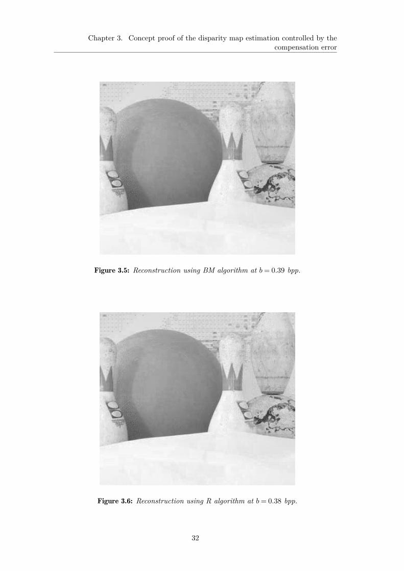
3.5 Reconstruction using BM algorithm at b= 0.39 bpp. . . . . . . . . . . . 32

3.6 Reconstruction using R algorithm at b= 0.38 bpp. . . . . . . . . . . . . 32

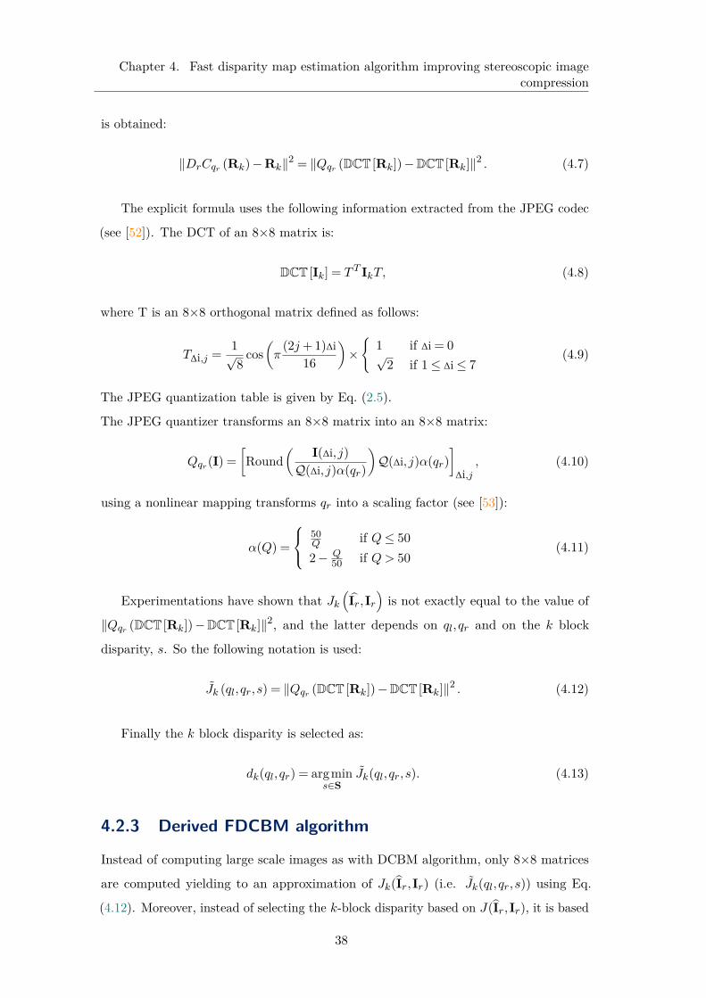
3.7 Reconstruction using DCBM algorithm at b= 0.38 bpp. . . . . . . . . . 33

4.1 Average distortion reduction ratio of BM-FDCBM compared to BM-

DCBM on synthetic data (function of qr). . . . . . . . . . . . . . . . . . 42

List of Figures

4.2 Performance comparison of BM, DCBM, FDCBM and R algorithms using

"Art" stereoscopic image of Middlebury-dataset (2005). . . . . . . . . . . 43

4.3 Reconstructed "Aloe" right view: BM algorithm (left side); R algorithm

(middle) and FDCBM algorithm (right side). . . . . . . . . . . . . . . . 44

4.4 Histogram of the disparity map yielded at b= 0.3bpp using "Aloe" stereo-

scopic image: BM algorithm (left side), R algorithm (on the middle) and

FDCBM algorithm (right side). . . . . . . . . . . . . . . . . . . . . . . . 44

4.5 Reconstructed "Dwarves" right view: BM algorithm (left side); R algo-

rithm (mid side) and FDCBM algorithm (right side). . . . . . . . . . . . 45

4.6 "Deimos-550-1" original right view. . . . . . . . . . . . . . . . . . . . . . 45

4.7 Close-up views of the reconstructed "Deimos-550-1" right view: BM

algorithm (left side); R algorithm (middle) and FDCBM algorithm (right

side). . . . . . . . . . . . . . . . . . . . . . . . . . . . . . . . . . . . . . . 45

4.8 Histogram of the increase in average PSNR-performance of FDCBM as

compared to BM, in terms of the number of stereoscopic images among

the 30 extracted from the 2005 and 2006 Middlebury-database. . . . . . 47

5.1 Performance comparison of BM, R, FDCBM and COMB algorithms on

the "Monopoly" stereoscopic image . . . . . . . . . . . . . . . . . . . . . 57

5.2 Performance comparison of BM, R, FDCBM and COMB algorithms using

"Ballon" stereoscopic image. . . . . . . . . . . . . . . . . . . . . . . . . . 58

5.3 "Monopoly" original right view. . . . . . . . . . . . . . . . . . . . . . . . 59

5.4 Histogram of the disparity map yielded at b= 0.33 bpp using Monopoly. 60

5.5 Reconstructed right view with the BM algorithm, (PSNR = 35.28dB,

SSIM = 0.95, b= 0.33bpp). . . . . . . . . . . . . . . . . . . . . . . . . . . 61

5.6 Reconstructed right view with the R algorithm (PSNR = 35.89dB, SSIM =

0.95, b= 0.33bpp). . . . . . . . . . . . . . . . . . . . . . . . . . . . . . . 62

5.7 Reconstructed right view with the FDCBM algorithm, (PSNR = 35.48dB,

SSIM = 0.95, b= 0.33bpp). . . . . . . . . . . . . . . . . . . . . . . . . . . 63

5.8 Reconstructed right view with the COMB algorithm, (PSNR = 36.58dB,

SSIM = 0.97, b= 0.33bpp). . . . . . . . . . . . . . . . . . . . . . . . . . . 64

xiv

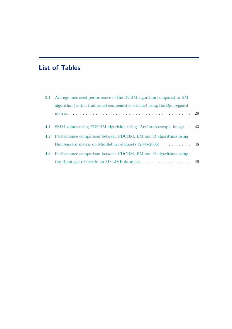
List of Tables

3.1 Average increased performance of the DCBM algorithm compared to BM

algorithm (with a traditional compensated scheme) using the Bjontegaard

metric. . . . . . . . . . . . . . . . . . . . . . . . . . . . . . . . . . . . . 29

4.1 SSIM values using FDCBM algorithm using "Art" stereoscopic image. . 43

4.2 Performance comparison between FDCBM, BM and R algorithms using

Bjøntegaard metric on Middlebury-datasets (2005-2006). . . . . . . . . 48

4.3 Performance comparison between FDCBM, BM and R algorithms using

the Bjøntegaard metric on 3D LIVE-database. . . . . . . . . . . . . . . 49

List of Tables

xvi

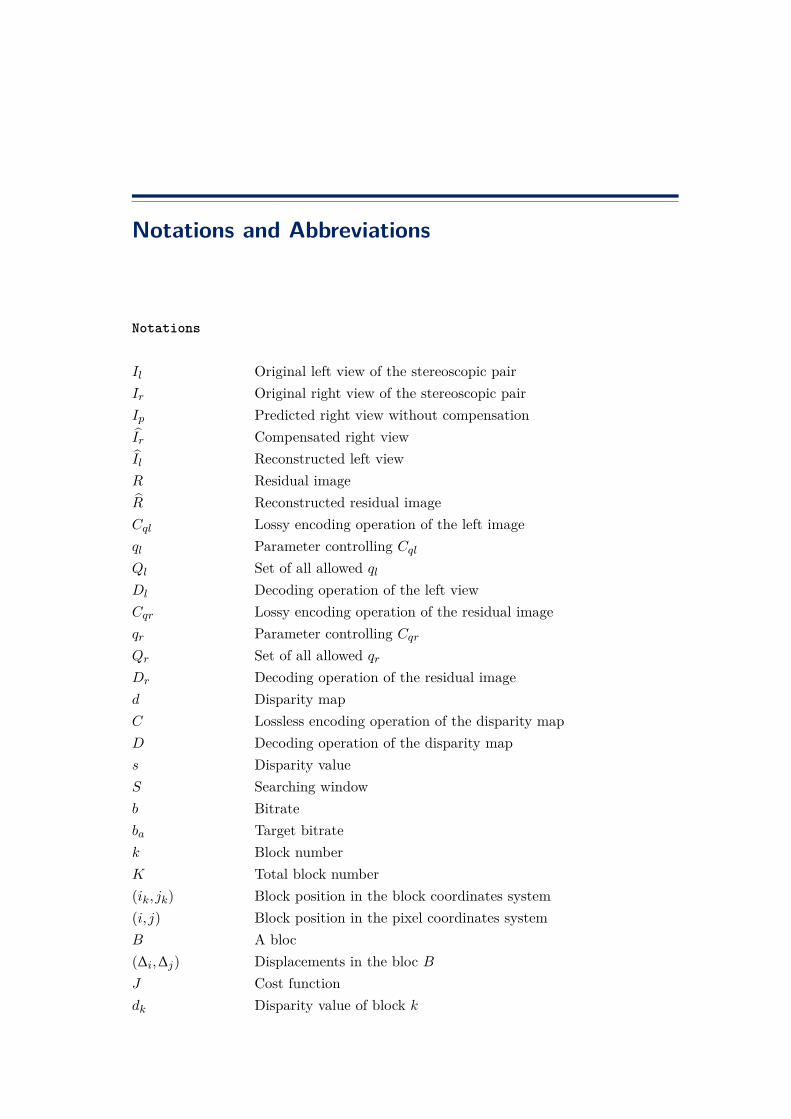
Notations and Abbreviations

Notations

Il Original left view of the stereoscopic pairIr Original right view of the stereoscopic pairIp Predicted right view without compensationIr Compensated right viewIl Reconstructed left viewR Residual imageR Reconstructed residual imageCql Lossy encoding operation of the left imageql Parameter controlling Cql

Ql Set of all allowed ql

Dl Decoding operation of the left viewCqr Lossy encoding operation of the residual imageqr Parameter controlling Cqr

Qr Set of all allowed qr

Dr Decoding operation of the residual imaged Disparity mapC Lossless encoding operation of the disparity mapD Decoding operation of the disparity maps Disparity valueS Searching windowb Bitrateba Target bitratek Block numberK Total block number(ik, jk) Block position in the block coordinates system(i, j) Block position in the pixel coordinates systemB A bloc(∆i,∆j) Displacements in the bloc BJ Cost functiondk Disparity value of block k

List of Tables

α Scaling factorT Orthogonal matrixρ(qr) Average distortion ratio (function of qr)

Abbreviations

PSNR Peak Signal to Noise RatioDC Disparity CompensationDCC Disparity Compensated Compression schemeDE Disparity EstimationIP Image PredictionBM Block MatchingDCBM Disparity Compensated Block MatchingFDCBM Fast Disparity Compensated Block MatchingCOMB Combining the R and FDCBM algorithmsDCT Discrete Cosine TransformIDCT Inverse Discrete Cosine Transform2D Two dimensional3D Three dimensionalAVC Advanced Video CodingMVV Multi View VideoMVC Multi View CodingStereo Stereoscopic

xviii

1

Ch

ap

te

r

Introduction

1.1 Thesis context

D uring the last decade, the use of stereoscopic imaging technology has greatly

increased. These images add the depth information which gives a more

realistic perceptual sensations. Many applications uses stereo imaging such

as 3D cinema, telemedecine, entertainment, cartography, remote sensing...

In fact, a stereoscopic pair is composed of two views (i.e. images) of the same

realistic-world scene with slightly different angles. The brain merges these two images

(i.e. left image and right image) to give the relief effect. This represents the fundamental

idea of stereoscopic vision.

Since the stereoscopic pair represents the same scene, the size of information is

doubled compared to the traditional 2D image. To deal with this issue, an efficient

compression technique is required to rapidly transmit and compactly store such data.

Similar to monoscopic coding technique, stereo image compression can exploit indepen-

dently the redundancy on each view. But thus doesn’t take advantage of the correlation

between the two images as their content is similar. In fact a pixel in the 3D scene

is projected onto two points respectively in the left and right views. The estimation

of the distance between all homologous pixels in each view forms the disparity map.

Hence to take advantage of the binocular dependency, a scheme based on the Disparity

Chapter 1. Introduction

Compensation (DC) is investigated and proposed in this thesis.

The principle of DC scheme is first to choose one of the two images as the reference

image (say the left image for instance). A disparity map is then estimated to predict

the target image (here the right image). After that a residual error is computed as the

difference between the original right view and its prediction. Finally the encoding left

image, the compressed residual and the lossless coding of the disparity map are sent to

the decoder side.

Estimating disparity map is very crucial in stereoscopic image coding because it

impacts the performance in terms of rate distortion. While the ground truth disparity

map is used for 3D reconstruction, The work of this manuscript focuses on disparity

estimation for stereoscopic image compression purpose. It is worth noting that the

disparity map accomplishing good performance can be different from the true disparity

map.

Note that this work was done in the context of a joint supervision contrat between

the Université Sorbonne Paris Nord (USPN) and the National Ingeneeing School of

Tunisia (ENIT). It is carried out between the L2TI (Laboratoire de Transport et

Traitement de l’Information) and LSITI (Laboratoire de Signal, Images et Technologies

de l’Information) laboratories.

1.2 Objectives and contributions

The objective of this PhD thesis concerns the improvement of stereoscopic image coding

algorithms of the state of the art. We are specially interested in improving the Disparity

Compensated Compression scheme. At the outline of our work is the idea that the

estimation of the disparity map should take into account, the impact of the encoded

residual error between the original image and its prediction to refine the predicted view,

instead of assuming that the best predicted view yields the best compensated one as it

is done in the state of the art.

Our main contributions are summarized as following:

While the classical Disparity Compensated Compression (DCC) scheme in most

cases based on Block Matching (BM) algorithm, yields a disparity map with which

the predicted image is most similar to its original version. Then, the residual error

2

computed between the original right view and its prediction version is encoded, yielding

a refinement added to the predicted image. In this manuscript, we propose a novel

approach which first, improves all the possible predicted images taking into account this

refinement, and then, estimates the disparity map as the one with which the predicted

image resembles most that same view. This strategy shows a proof-of-concept work

that selecting disparities according to the compensated view instead of the predicted

view improves the rate-distortion performance. But this is done at the expense of the

significant increase in numerical complexity.

To overcome this drawback, an other contribution concerns the computation of the

blockwise disparity using a simplified model of how the encoder used for the residual

error deals with the compensation refinement. This computation is done with the

derived analytic expression exploiting in what causes distortion in such coder, namely

the quantization of the DCT components as in JPEG coder. Indeed, disparity selection

is no longer based on the computation of the whole compensated view with all its

pixel values. Only 8× 8 pixel values of the residual error are taken into account. Thus

numerical complexity is definitely reduced. Basically disparity related blocks are exactly

the JPEG related blocks (8× 8). Our algorithm can be extended to larger blocks.

The aim of our last contribution is to select the disparity map accomplishing the best

trade off between the minimization of the bitrate allocated to the disparity map and the

minimization of the distortion of the predicted view. For this, the proposed strategy

consists in combining two existing algorithms. The first one, called R-algorithm [1]. It

is more efficient at low bitrates The second one, is already described in the previous

contribution. It performs better at high bitrates.

1.3 Organization of the thesis

This dissertation is organized as follows.

Chapter 2 describes first the basic notions of stereo vision specially the principle of

stereoscopic vision, the geometrical models used by stereoscopic systems and the methods

used to compute disparities. Then we give an overview of stereoscopic image coding.

Chapter 3 shows how finding the best performing disparity map can be regarded

as solving an optimization problem. The classical BM algorithm is derived as a

sub-optimal solution. Then we describe the proposed Disparity Compensated Block

3


Matching (DCBM) algorithm as an other sub-optimal solution which takes into account

the compensation effect. Simulations results are presented to compare the developed

algorithm with the the classical BM approach with compensation. Due to its good

performance in terms of rate-distortion, this chapter is a good proof of the proposed

concept which, to our knowledge, has not been proposed in the state of the art.

Chapter 4 is concerned with finding the optimal solution to the optimization problem

to solve, in particular, the computational complexity of the developed algorithm intro-

duced in the previous chapter. A fast version of the DCBM, called FDCBM algorithm,

by approximating the distortion between blocks of the compensated image and its

original version by blocks of decoded residual error and its original version is proposd.

This is thanks to an adequate modelling of the JPEG coding. This algorithm is also

extended to blocks larger than 8×8 pixels. Experiments show that our proposal performs

better than the BM with compensation, DCBM algorithms and another algorithm of

the state of the art.

Chapter 5 proposes to combine the developed FDCBM algorithm and an existing

algorithm of the sate of the art. The proposed algorithm called COMB, jointly optimizes

the bitrate and the distortion.

Finally, Chapter 6 concludes this manuscript and gives some directions for further

investigation.

1.4 Publications

• International journal paper

I. Kadri, G. Dauphin, A. Mokraoui and Z. Lachiri, Disparities selection controlled

by the compensated image quality for a given bitrate, Signal, Image and Video

Processing, February 2020, DOI 10.1007/s11760-020-01643-1.

• International conference paper

I. Kadri, G. Dauphin, A. Mokraoui and Z. Lachiri, Stereoscopic Image Coding

Performance using Disparity-Compensated Block Matching Algorithm, Signal

Processing: Algorithms, Architectures, Arrangements and Applications (IEEE

SPA conference), Poznan, Poland, 2019.

4

I. Kadri, G. Dauphin, A. Mokraoui and Z. Lachiri, Stereoscopic image coding

using a global disparity estimation algorithm optimizing the compensation scheme

impact, Signal Processing: Algorithms, Architectures, Arrangements and Applica-

tions (IEEE SPA conference), Poznan, Poland, 2020 (Submitted).

• National conference paper

I .Kadri, G. Dauphin, A. Mokraoui, Z. Lachiri, Algorithme d’appariement de

blocs basé sur l’optimisation de la compensation de disparité pour le codage

d’image stéréoscopique, Compression et Représentation des Signaux Audiovisuels

(CORESA), 12-14 Novembre 2018, Poitiers.

5


6

2

Ch

ap

te

r

State of the art on stereoscopic image coding

Summary

O ver the last decade, the use of stereo imaging technology has significantly

increased. Applications concerns the entertainment, industry, medical fields

and cartography. A stereo image is composed of two views (left and right)

perceived as two viewpoints of the same scene. Consequently, the amount of information

to be stored or transmitted is doubled compared to the monoscopic image. That’s why

it is important to efficiently encoding them.

This chapter outlines the basic notions to understand the stereoscopic imaging. Firstly,

we introduce the fundamental aspects of stereo vision. Secondly, we present an overview

of stereoscopic image coding.

2.1 Stereoscopic vision aspects

2.1.1 Related concepts

Stereopsis results from the fusion of two pictures presented to the brain from left and

right eyes as shown in Fig. 2.1. Each eye looks at the real scene from a slightly different

perspective. The merging of these two images gives a depth sense (3D perception).

To mimic the human visual system the easiest way is to put two cameras side by side

with a side shifting for acquiring left and right images of the same scene. Fig. 2.2

Chapter 2. State of the art on stereoscopic image coding

Figure 2.1: Binocular vision (source: [2]).

presents an example of stereo camera system.

Figure 2.2: Stereoscopic camera (source: [3]).

2.1.2 Stereoscopic geometry/systems of stereo acquisition

In order to describe image acquisition, the simplest model is the pinhole (linear projective)

one. This model is illustrated in Fig. 2.3. It is composed by a retinal plane Ωr where

the image is formed, an optical center o placed at a focal distance f of the optical

system. This system is contained in the focal plane Ωf . The optical axis passes through

the center of projection O. This line is perpendicular to Ωr In fact, it has demonstrated

8

Figure 2.3: Pinhole camera model (source: [4]).

that the camera pinhole model can approximate efficiently the geometry and optics of

most modern cameras [4]. It maps 3D point P(X,Y,Z) to 2D point p(x,y) as:

x= fX

Z,y = f

Y

Z(2.1)

where f is the focal distance

2.1.2.1 Epipolar constraint

Epipolar geometry describes the relationship between homologous points in left and

right images. The different elements involved in this geometry are depicted in Fig . 2.4.

The epipolar plan Ω contains optical centers of left and right camera respectively Ol

and Or, the 3D point P and its projection Pl and Pr. The baseline is the line joining

the camera centers. The two points el and er result from the intersection of the baseline

with the image plane are called epipoles. Let us now consider only the left projection

Pl and we search for its correspondant point in the right image. The point P belongs

necessarly to the line OlPl. The right projection Pr is located on the line lr where the

epipolar plane intersect the right image (due to the co-planarity). This line refers to

the epipolar line associated to Pr (similarly for ll the conjugate epipolar line). Not that

all the epipolar lines in the image pass through the epipole point.

After explaining the geometric aspect of the epipolar constraint, we present the

9


Figure 2.4: Epipolar geometry (source: [5]).

algebraic aspect, formalized by the fundamental matrix F as:

PrFTPl = 0 (2.2)

F is a 3×3 matrix depending on the intrinsic and extrinsic parameters of the cameras

[6, 7]. By intrinsic parameters we mean the optical geometric, and digital characteristics

of the camera and by extrinsic parameters orientations and positions of each camera.

For detailed description of estimation techniques of the fundamental matrix, a complete

review is cited in [7].

To recapitulate, the epipolar constraint overcome the complexity of searching homologous

points. The search filed is restricted to 1D lines instead of the whole 2D image. This

process is called rectification.

2.1.2.2 Rectification

In stereoscopic vision we distinguish mailly two camera dispositions. Fig. 2.4 illustrates

the first configuration in which cameras are rotated towards each others by a small

angle. This angle gives an inclination of epipolar lines. In the second camera disposition,

the optical axes of cameras as well epipolar lines are parallel. Those latter coincide with

the scanning lines as depicted in Fig . 2.5. This simplify the correspondence search.

So homologous points have the same vertical coordinate. Indeed, rectification is the

process that converts the first configuration to the simplified second one by involving

transformation which projects the two images onto the same plane. A survey of the

diverse existing rectification methods can be found in [8–10].

10

Figure 2.5: Epipolar rectification (source: [5]).

2.1.3 Methods of disparity estimation

Despite the reduction of the research field for correspondent points with epipolar

geometry, it does not give any information about the exact location of both homologous

points. Indeed, disparity is the difference in the x-coordinates of the corresponding

pixels in the left and right views. Dense disparity map results from carrying out stereo

matching for all pixels. After that, depth in 3D space is derived from this spatial shift.

The literature divides disparity estimation methods mainly into two classes: local and

global disparity estimation methods.

2.1.3.1 Local stereo correspondence methods

Local methods measure the similarity between two sets of pixels. They can be basically

subdivided into two approaches: feature based approaches and area based ones. In

the first category, high level feature like edges [11], curves [12] or segments [13] are

compared.These features represent geometric properties of a scene which makes these

methods accurate. Nevertheless, the step of feature extraction should be involved.

Another disadvantage is related to the sparsity of the estimated disparity map which

requires an interpolation step to complete disparities. This is not the case with area

based algorithms which estimate directly a dense disparity map. This kind of methods

is efficient in highly textured regions but sensitive to locally ambiguous zones due for

example to occlusion and textureless contents. Area based methods correlate pixels

or regions. That’s why they are known as correlation-based approaches. Its principle

is depicted in Fig. 2.5. Let us consider a pixel Pr in the right image. How can we

find its homologous point in the left image? We start by selecting a window/bloc

11


surrounding Pr. After that, this bloc is moved in the left image search area to search

a match window. At every shift a cost function is computed. Finally, the retained

Figure 2.6: Correlation-based stereo matching approaches (source: [5]).

match is the one that gives the lowest cost. Many similarity measures can be used such

as the Sum of Square Differences (SSD), the Sum of Absolute Differences (SAD) and

the Normalized Cross-Correlation (NCC). The choice of window size and shape is the

main inconvenient of correlation based methods. To overcome this limitation many

approaches have been proposed which consider variable shape and size adaptively to

the pixels intensity variation in the image [14–16].

2.1.3.2 Global stereo correspondence methods

Global methods aim at minimizing a global energy function E(d) to estimate the

disparity map. This latter defines the cost based on the measure of the displacement

between correspondent pixels Edata(d) and a regularization term Esmooth(d) called

smoothing prior which carries on the smoothness of the final disparity map. E(d) takes

the following form:

E(d) = Edata(d) +αEsmooth(d) (2.3)

where α is a positif term and d the estimated disparity map.

Dynamic programming (DP) [17, 18] is one of the most commonly used global methods.

Its principle is as following: Let’s take two scanlines (with the epipolar constraint) of

size L. First a LxL cost matrix for all possible matching pixels is built. Then, best

matchs are selected taking into account the ordering and smoothness constraints. But

12

DP suffers from the well-known streaking effects which consist on the inconsistency

problem between horizontal and vertical scanlines. To overcome this limitation a two

pass dynamic programming has been proposed in [18].

To cope with the streaking artifacts, Roy and Cox [19] have proposed graph cuts methods.

Its underlying idea is to transform the stereo problem in a pixel labelling one in order to

construct a graph with minimal cut. Variational approaches [20] and belief propagation

[21] are also used as techniques for global methods.

2.2 Reviewing the state of the art on stereoscopicimage compression

Before presenting the overview on stereo image coding, let us give some background on

image compression.

2.2.1 Basic concepts of image compression

The goal of compression is the reduction of the bits’ number needed to represent an

image. They are either lossless or lossy compression approaches. In lossless compression

approaches, the decoded image is exactly the same as its original version. Contrary to

the lossy compression approaches, the decoded image is an approximation of the original

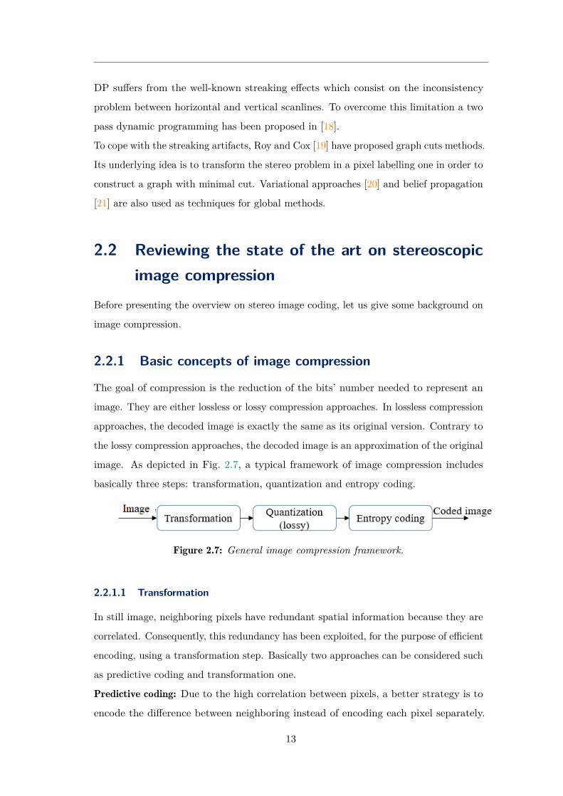
image. As depicted in Fig. 2.7, a typical framework of image compression includes

basically three steps: transformation, quantization and entropy coding.

Figure 2.7: General image compression framework.

2.2.1.1 Transformation

In still image, neighboring pixels have redundant spatial information because they are

correlated. Consequently, this redundancy has been exploited, for the purpose of efficient

encoding, using a transformation step. Basically two approaches can be considered such

as predictive coding and transformation one.

Predictive coding: Due to the high correlation between pixels, a better strategy is to

encode the difference between neighboring instead of encoding each pixel separately.

13


The most common approach is Differential Pulse Code Modulation (DPCM) [22].

Transform coding: Redundancy in the transform domain is reduced greatly. So it’s

more efficient to code an image in its transformed version than in its original one. The

Discrete Cosine Transform (DCT) [23] and the Discrete Wavelet Transform (DWT) [24]

are the most used transforms in image and video compression.

The DCT transforms an image from its spatial representation to the frequency one. It has

been used in different image/video coding standards such as JPEG (Joint Photographic

Experts Group) [25] and MPEG coding standards (H263 [26], H264 [27], HEVC [28]) .

The DCT, as a block transform, operates as following. The image is divided into non

overlapping blocks for example 8× 8 pixels and then the DCT is applied.The main

drawback of DCT is the blocks’ artifacts at low bitrates. On the other hand, DWT

overcomes the drawbacks of the DCT. It is used in the JPEG 2000 standard [29].

Wavelet gives a representation in the spatial and scale domains of the image.

2.2.1.2 Quantization

Quantization is an irreversible operator (lossy). It converts a continuous signal into

a discrete one. Two classes of quantization can be defined: vector and scalar. While

vector quantization operates on blocks of transform coefficients, scalar quantization

treats independently transform coefficients one by one.

It is worth pointing out that scalar quantization is less complex and is frequently used

in practice. It can be used in two ways. Uniform quantization is suitable when the

coefficients to be quantized are uniformly distributed. They are separated by a fixed

distance called quantization step Q50. Then the quantization is given by:

∀x ∈ R f(x) =Q50×[x

Q50

](2.4)

where [.] is the round operator and x (i.e. the coefficient) a real number. On the other

hand,for non distributed coefficients, adaptive quantization should be performed. It is

14

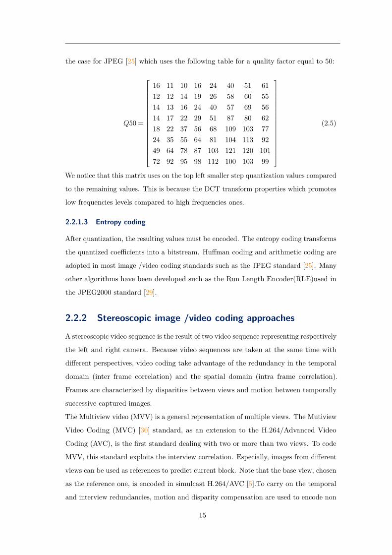
the case for JPEG [25] which uses the following table for a quality factor equal to 50:

Q50 =

16 11 10 16 24 40 51 6112 12 14 19 26 58 60 5514 13 16 24 40 57 69 5614 17 22 29 51 87 80 6218 22 37 56 68 109 103 7724 35 55 64 81 104 113 9249 64 78 87 103 121 120 10172 92 95 98 112 100 103 99

(2.5)

We notice that this matrix uses on the top left smaller step quantization values compared

to the remaining values. This is because the DCT transform properties which promotes

low frequencies levels compared to high frequencies ones.

2.2.1.3 Entropy coding

After quantization, the resulting values must be encoded. The entropy coding transforms

the quantized coefficients into a bitstream. Huffman coding and arithmetic coding are

adopted in most image /video coding standards such as the JPEG standard [25]. Many

other algorithms have been developed such as the Run Length Encoder(RLE)used in

the JPEG2000 standard [29].

2.2.2 Stereoscopic image /video coding approaches

A stereoscopic video sequence is the result of two video sequence representing respectively

the left and right camera. Because video sequences are taken at the same time with

different perspectives, video coding take advantage of the redundancy in the temporal

domain (inter frame correlation) and the spatial domain (intra frame correlation).

Frames are characterized by disparities between views and motion between temporally

successive captured images.

The Multiview video (MVV) is a general representation of multiple views. The Mutiview

Video Coding (MVC) [30] standard, as an extension to the H.264/Advanced Video

Coding (AVC), is the first standard dealing with two or more than two views. To code

MVV, this standard exploits the interview correlation. Especially, images from different

views can be used as references to predict current block. Note that the base view, chosen

as the reference one, is encoded in simulcast H.264/AVC [5].To carry on the temporal

and interview redundancies, motion and disparity compensation are used to encode non

15


base view [5] as described in the following section.

2.2.3 Disparity compensated scheme

Stereoscopic images present similar contents from slightly different perspective and the

spatial displacements yield to the disparity map. In the purpose of exploiting inter-image

redundancies more efficient coding schemes have been proposed based on the disparity

compensation (DC) technique which is analog to motion compensation scheme used in

video coding [31]. The DC process involves the main following steps:

(i) One of the two views is taking as the reference one (for example the left one).

(ii) A disparity map is then estimated between the left and right images.

(iii) The target image (the right one) is then predicted based on the estimated disparity

map.

(iv) A residual image is computed as the difference between the original right view

and its prediction.

(v) This residual error is added to the predicted view in order to find the reconstructed

target image by compensation.

The reference view and the residual error are encoded after a transformation coding.

The disparity map is lossless encoded using an entropy coder. Finally, these information

are sent to the decoder in order to recover the stereo pair.

Two stereoscopic coding schemes are proposed in the literature: Open Loop (OL) based

structure and Closed Loop (CL) based structure. They are shown respectively in Fig. 2.8

and Fig. 2.9. They differ in the disparity estimation level.

As illustrated in Fig. 2.8, in the OL case, disparity map computation considers the

original left view. This is not the case with the CL case which use the decoded left view

as depicted in Fig. 2.9.

When decoding, whatever the structure, the left view is decoded at the beginning. The

right view is then predicted based on the decoded left image and disparity map. To

obtain the final reconstructed right view, the decoded residual error is added to the

predicted right view (the compensation). When using the OL scheme, the reference

view at the encoder and decoder are different which makes this structure sub-optimal.

16

Figure 2.8: Open Loop for stereoscopic image coding scheme [32].

Figure 2.9: Closed Loop for stereoscopic image coding scheme [32].

To deal with this problem, the CL scheme use the decoded reference view at coding and

decoding sides.

2.2.4 Disparity estimation for stereo image coding

The estimation of the disparity map is a crucial operation because it has an impact

on the performance of the compressed stereoscopic image in terms of rate-distortion.

Blockwise disparity is usually used because one disparity value is assigned to all pixels

of the same block requiring therefore a few bit budget to encode the stereoscopic image.

Indeed, several coding algorithms are based on the disparity compensated scheme. In

17


[33], disparity map is sequentially estimated minimizing a joint entropy distortion metric

modelling the compromise between the minimization of the distortion of the predicted

image (before compensation) and the minimization of the entropy needed to encode

the disparity map. This is achieved by building a tree where each path represents a

partial disparity map. This proposal extends only the M best paths, at at each depth,

by all possible disparities. This algorithm is also extended for non rectified stereoscopic

image in [34]. The proposal in [35] is an extension of [33] which considers also blocks of

variable sizes. In [1], Kadaikar and al. estimate also the disparity map using the same

entropy distortion metric. Disparity map yielded by the BM algorithm is first taken

as the reference one. This initial map is successfully modified when improvements are

possible in terms of rate distortion.

Two approaches are proposed, in [36], for selecting disparities, from a large search

window, minimizing the predicted image distortion for a given bitrate. The initial

disparity map is the one computed by the BM algorithm. In [35], a new method for

estimating disparity map using blocks of variable size is developed. This is by reducing

the prediction view distortion and the bitrate needed to encode the disparity and the

block length maps.

A region-based scheme for stereo image coding is presented in [37]. Basically occluded

and non occluded regions are considered. Occluded ones are independently encoded.

Whereas non occluded regions are segmented firstly into edge and smooth zones. Then

they are divided in blocks of fixed size to be used in the block matching algorithm.

Disparity map is losslessly encoded using residual uniform scalar quantizer followed by

an adaptive arithmetic encoder.

Furthermore, disparity estimation and compensation are done after the DCT transfor-

mation of the right and let images in [38]. In [39] presents a wavelet-based stereo image

coding scheme is proposed. Before disparity estimation and compensation a wavelet

transform is applied to the stereo pair. To encode the wavelt coefficients a Subspace

Projection Technique (SPT) is performed. Authors in [40] presented a method where

disparity map and residual error are computed in the bandlet domain. In [41] a joint

coding scheme using the Vector Lifting Scheme (VLS) to represent the stereoscopic pair

instead of residual error is presentd. The generated dense and smooth disparity map is

then integrated in the VLS scheme.

18

ConclusionThis chapter presented the main concepts of stereoscopic imaging. A review of previous

work on stereoscopic image coding approaches using the disparity compensated technique

has been given.The following chapters will present our contributions on stereoscopic

image coding.

19


20

3

Ch

ap

te

r

Concept proof of the disparity map estimation con-trolled by the compensation error

Summary

T he main objective of this chapter is to confirm the relevance of the new

strategy of estimating the disparity map when the stereoscopic coding is

based on a compensation scheme. The DC classical approach is based on

Block Matching (BM) algorithm, yielding a disparity map with which the predicted image

is most similar to its original version. Then, with no modification of the disparity map,

the residual error is encoded, yielding a refinement added to the predicted image. Our

proposal improves all the possible predicted images taking into account this refinement,

and then, estimates the disparity map as the one with which the predicted image after

compensation resembles most to its original version.

The remainder of this chapter is organized as follows. First, we present the optimization

problem. Then we provide the description of the proposed algorithm. After that,

experimental results are illustrated. Finally conclusions are drawn. This contribution

resulted in an international and national conferences [42, 43].

Chapter 3. Concept proof of the disparity map estimation controlled by thecompensation error

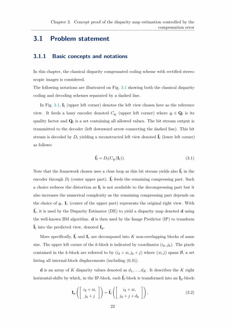
3.1 Problem statement

3.1.1 Basic concepts and notations

In this chapter, the classical disparity compensated coding scheme with rectified stereo-

scopic images is considered.

The following notations are illustrated on Fig. 3.1 showing both the classical disparity

coding and decoding schemes separated by a dashed line.

In Fig. 3.1, Il (upper left corner) denotes the left view chosen here as the reference

view. It feeds a lossy encoder denoted Cql (upper left corner) where ql ∈ Ql is its

quality factor and Ql is a set containing all allowed values. The bit stream output is

transmitted to the decoder (left downward arrow connecting the dashed line). This bit

stream is decoded by Dl yielding a reconstructed left view denoted Il (lower left corner)

as follows:

Il =Dl(Cql(Il)). (3.1)

Note that the framework chosen uses a close loop as this bit stream yields also Il in the

encoder through Dl (center upper part). Il feeds the remaining compressing part. Such

a choice reduces the distortion as Il is not available to the decompressing part but it

also increases the numerical complexity as the remaining compressing part depends on

the choice of ql. Ir (center of the upper part) represents the original right view. With

Il, it is used by the Disparity Estimator (DE) to yield a disparity map denoted d using

the well-known BM algorithm. d is then used by the Image Predictor (IP) to transform

Il into the predicted view, denoted Ip.

More specifically, Il and Ir are decomposed into K non-overlapping blocks of same

size. The upper left corner of the k-block is indicated by coordinates (ik, jk). The pixels

contained in the k-block are referred to by (ik + ∆i, jk + j) where (∆i, j) spans B, a set

listing all internal-block displacements (including (0,0)).

d is an array of K disparity values denoted as d1, . . . ,dK . It describes the K right

horizontal-shifts by which, in the IP-block, each Il-block is transformed into an Ip-block:

Ip

([ik + ∆i,jk + j

])= Il

([ik + ∆i,

jk + j+ dk

]), (3.2)

22

where k ranges from 1 to K and (∆i, j) spans B. This IP-block is shown on the upper

right part in Fig. 3.1. To simplify notations, we do not indicate here the d-dependency

of Ip.

The BM algorithm, in the DE block, consists in selecting for each k-block, the

disparity value dk for which the k-block Ip-values resemble most the k-block Ir-values

in the sense that the mean squared error is minimized as follows:

dk(ql) = arg mind∈S

∑(∆i,j)∈B

(Il

[ik +∆i

jk + j+ d

]− Ir

[ik +∆ijk + j

])2

, (3.3)

where S contains all allowed disparity values. As Il is ql-dependent, the disparity value

found, dk is also ql-dependent. C (center upper part) is a lossless encoding operation

of the disparity map d. The resulting bit stream is transmitted to the decoder (center

downward arrow connecting the dashed line) which recovers the exact disparity map d,

through D, being the inverse operation of C as follows:

d =D(C(d)). (3.4)

The recovered disparity map is used with Il by the second IP-block to yield according

to Eq. (3.2), Ip, this time in the decoder. This second IP-block is at the bottom in

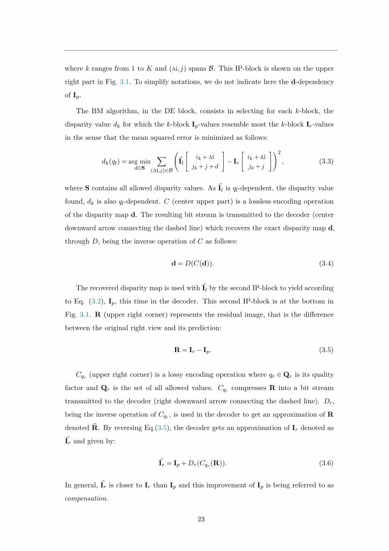
Fig. 3.1. R (upper right corner) represents the residual image, that is the difference

between the original right view and its prediction:

R = Ir − Ip. (3.5)

Cqr (upper right corner) is a lossy encoding operation where qr ∈Qr is its quality

factor and Qr is the set of all allowed values. Cqr compresses R into a bit stream

transmitted to the decoder (right downward arrow connecting the dashed line). Dr,

being the inverse operation of Cqr , is used in the decoder to get an approximation of R

denoted R. By reversing Eq.(3.5), the decoder gets an approximation of Ir denoted as

Ir and given by:

Ir = Ip +Dr(Cqr (R)). (3.6)

In general, Ir is closer to Ir than Ip and this improvement of Ip is being referred to as

compensation.

23


The bitrate, denoted b, is deduced from the bit streams Cql(Il), C(d) and Cqr (R):

b(Il,d,Ir, ql, qr) = |Cql(Il)|+ |C(d)|+ |Cqr (R)||Il|+ |Ir|

, (3.7)

where | .| is the set cardinal number, here it helps counting, above, the number of bits,

and below, the number of pixels.

Figure 3.1: Disparity compensated coding scheme where the encoder (above) isseparated from the decoder (below) by a dashed line.

3.1.2 Optimization problem statement

The aim of a coding/decoding scheme is a trade-off between getting the highest quality

(e.g. visual rendering) while using the least amount of bits accounted for by Eq. (3.7).

Here this trade-off is rephrased into finding the best quality (i.e. visual rendering) within

a constrained bit-budget. As the end user observing the reconstructed stereoscopic

image is generally a human being, our focus should be the extent to which the visual

experience is being preserved. Designing objective quality metric modelling the quality

of this visual experience is an existing research field as exemplified in [44]. As of

now, no objective quality metric has proven to be completely reliable when applied to

stereoscopic images. We are considering a quality metric, denoted as J to be used as a

cost function in an optimization problem. It is for the sake of simplifying the description

of the proposed algorithm is in section 3.2. As a consequence, at the coder level the

choice of ql, qr,d should within a constrained bit-budget minimize J . Generally, the

24

cost function of an image I′ as compared to an image I is:

J(I′,I

)= 1K

K∑k=1

Jk(I′,I

). (3.8)

where Jk is the cost function of the k-block.

Numerical complexity being an important issue, the two following assumptions seem to

be required to make this optimization problem tractable:

A1) Up to a non decreasing or non-increasing mapping, J is the sum of a metric

computed independently on each blocks of Ir and Ir and a metric computed on Il

and Il.

A2) The bitrate control is addressed solely by selecting ql and qr.

With these assumptions and denoting ba the allowed bit-budget, the optimization

problem addressing the optimal choice of ql, qr,d at the coder level is:

d(ql, qr) = argmind∈SK

J(Ir(ql, qr,d),Ir) (3.9)

J (Il,Il, Ir,Ir) = 12J(Il,Il

)+ 1

2J(Ir,Ir

)(3.10)

(ql, qr) = argminql∈Ql, qr∈Qr, b≤ba

J(Il(ql),Il, Ir(ql, qr,d(ql, qr)),Ir

), (3.11)

where b, defined in Eq. (3.7), depends on Il,d,Ir, ql, qr. SK is the set of all arrays of

size K whose components are in S and ba is the expected bitrate.

Investigating the link between the BM algorithm and this optimization problem, Eq.

(3.3) is recasted into:

dk(ql) = argmins∈S

Jk(Ip,Ir). (3.12)

When considering the whole array of disparities, Eq. (3.12) becomes:

d(ql) = argmind∈SK

J(Ip,Ir). (3.13)

Let us now suppose that the objective quality metric chosen is the PSNR (Peak

25


Signal to Noise Ratio) whose specific definition for stereoscopic images is:

PSNR(Il, Il,Ir, Ir) =

10log10

(2552(|Il|+|Ir|)∑

i,j(Il(i,j)−Il(i,j))2+

∑i,j

(Ir(i,j)−Ir(i,j))2

),

(3.14)

where pixel values are ranging from 0 to 255, i, j span all pixel positions and |Il|, |Ir|

denote the number of pixels.

Hence, the BM algorithm can be regarded as a suboptimal solution of Eq. (3.10),

where the effect of the choice of the disparity on the residual, and the residual impact on

the distortion, are neglected. Note that from then on, this DCC algorithm is referred to

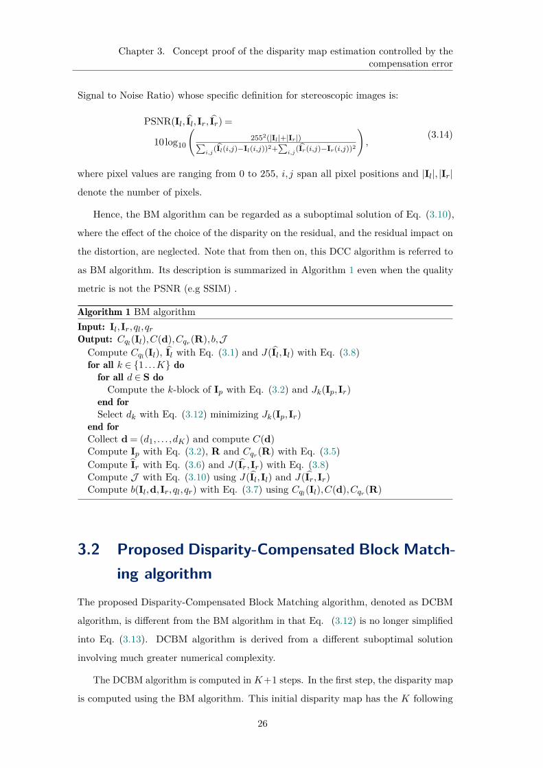
as BM algorithm. Its description is summarized in Algorithm 1 even when the quality

metric is not the PSNR (e.g SSIM) .

Algorithm 1 BM algorithmInput: Il,Ir, ql, qr

Output: Cql(Il),C(d),Cqr (R), b,JCompute Cql(Il), Il with Eq. (3.1) and J(Il,Il) with Eq. (3.8)for all k ∈ 1 . . .K do

for all d ∈ S doCompute the k-block of Ip with Eq. (3.2) and Jk(Ip,Ir)

end forSelect dk with Eq. (3.12) minimizing Jk(Ip,Ir)

end forCollect d = (d1, . . . ,dK) and compute C(d)Compute Ip with Eq. (3.2), R and Cqr (R) with Eq. (3.5)Compute Ir with Eq. (3.6) and J(Ir,Ir) with Eq. (3.8)Compute J with Eq. (3.10) using J(Il,Il) and J(Ir,Ir)Compute b(Il,d,Ir, ql, qr) with Eq. (3.7) using Cql(Il),C(d),Cqr (R)

3.2 Proposed Disparity-Compensated Block Match-ing algorithm

The proposed Disparity-Compensated Block Matching algorithm, denoted as DCBM

algorithm, is different from the BM algorithm in that Eq. (3.12) is no longer simplified

into Eq. (3.13). DCBM algorithm is derived from a different suboptimal solution

involving much greater numerical complexity.

The DCBM algorithm is computed in K+1 steps. In the first step, the disparity map

is computed using the BM algorithm. This initial disparity map has the K following

26

components:

dk(0, ql) = argmind∈S

Jk (Ip,Ir) , (3.15)

where k ranges from 1 to K. Note that at this point d(0, ql) does not depend on qr.

The goal at step t ∈ 1, . . . ,K is to select the k-block disparity, denoted, for now,

as s. We assume that a disparity map d(t− 1, ql, qr) has already been computed at step

t− 1. For each s ∈ S, a predicted image Ip(t,ql, qr,s) is computed taking into account s

on the tth block and dk(t− 1, ql, qr) for all other blocks:

Ip(t,ql, qr,s)[ik + ∆ijk + j

]=

Il

[ik + ∆i

jk + j+ dk(t− 1, ql, qr)

]if k , t

Il

[ik + ∆i

jk + j+ s

]if k = t

(3.16)

with (∆i, j) spanning B and k ranging from 1 to K.

Compensation transforms Ip(t,ql, qr,s) into Ir(t,ql, qr,s) as follows:

Ir(t,ql, qr,s) = Ip(t,ql, qr,s) +DrCqr (Ir − Ip(t,ql, qr,s)) . (3.17)

Finally J(Ir,Ir) is computed and the best disparity is selected as follows:

dk(t,ql, qr) =

dk(t− 1, ql, qr) if k , targmin

s∈SJ(Ir(t,ql, qr,s),Ir

)if k = t

(3.18)

The DCBM algorithm is summarized in algorithm 2.

Note that the increased numerical complexity when using DCBM, stems from the

necessity, to code and decode a new image, at each block and then each time a new

disparity value is considered.

27


Algorithm 2 DCBM algorithmInput: Il,Ir, ql, qr

Output: Cql(Il),C(d),Cqr (R), b,JCompute Cql(Il), Il with Eq. (3.1) and J(Il,Il) with Eq. (3.8)Compute d(0, ql) with Eq. (3.15) using Ip defined by Eq. (3.2)for all t ∈ 1 . . .K do

for all s ∈ S doCompute Ip(t,ql, qr,s) with Eq. (3.16) using d(t− 1, ql, qr)Compute Ir(t,ql, qr,s) with Eq. (3.17)Compute J

(Ir(t,ql, qr,s),Ir

)with Eq. (3.8)

end forSelect d(t,ql, qr) with Eq. (3.18) using all s-values of J(Ir,Ir)

end forGet d = d(K,ql, qr) and compute C(d)Compute Ip with Eq. (3.2) using dCompute R = Ir − Ip and Cqr (R) with Eq. (3.5)Compute Ir with Eq. (3.6) and J(Ir,Ir) with Eq. (3.8)Compute J with Eq. (3.10) using J(Il,Il) and J(Ir,Ir)Compute b(Il,d,Ir, ql, qr) with Eq. (3.7) using Cql(Il),C(d),Cqr (R)

3.3 Experiments and results

The performance of the proposed DCBM algorithm is compared to the BM and R

[1] algorithms with a traditional compensation scheme on some stereoscopic images

extracted from the Middleburry database [45] and the Deimos dataset [46].

In these experiments, the PSNR (defined in Eq. (3.14)) is used both as a performance

measure and as the cost function used in the algorithms. To reduce the important

amount of computations, the left view is not encoded and the PSNR is computed using

only Ir and Ir with a simplified definition.The Structural Similarity Index (SSIM) [47]

is also used to evaluate the performance. The bitrate in bit per pixel (bpp) takes

into account the amounts of bits to encode d and R and Eq. (3.7) is modified into:

b(d,Ir) = |C(d)|+|Cqr (R)||Ir| . Arithmetic coding [48] has been chosen to encode d and JPEG

(i.e. DCT and quantization) to encode the R. To reduce the numerical complexity, the

available range of JPEG hyperparameter values has been reduced in Qr to 10,20, . . . ,90.

Of great importance is the choice of the block size, set to 8×8 as it matches the JPEG-

block size. Pixel values are ranging from 0 to 255. The searching window S is, unless

otherwise specified, −14, . . . ,15.

Table 3.1 compares the performance of the DCBM algorithm to the BM algorithm using

28

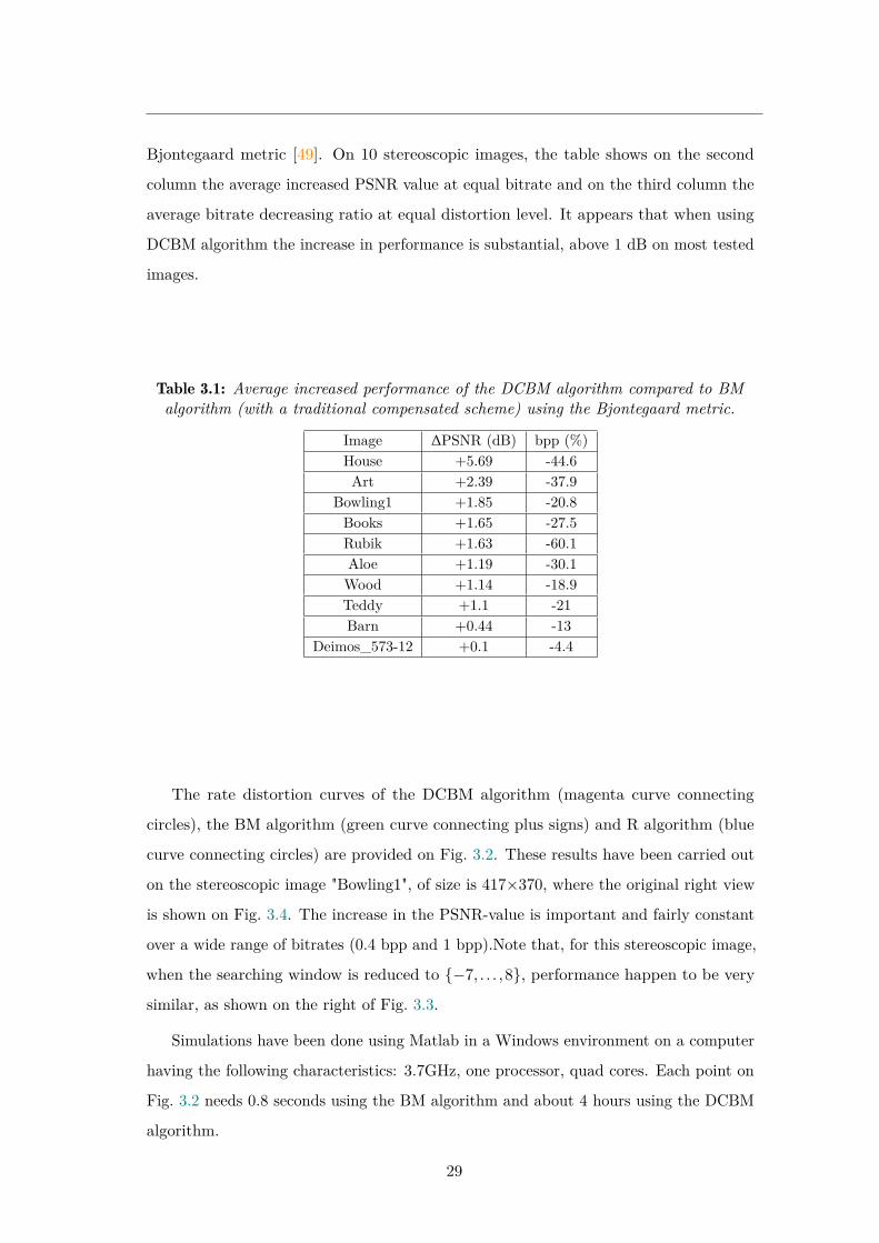
Bjontegaard metric [49]. On 10 stereoscopic images, the table shows on the second

column the average increased PSNR value at equal bitrate and on the third column the

average bitrate decreasing ratio at equal distortion level. It appears that when using

DCBM algorithm the increase in performance is substantial, above 1 dB on most tested

images.

Table 3.1: Average increased performance of the DCBM algorithm compared to BMalgorithm (with a traditional compensated scheme) using the Bjontegaard metric.

Image ∆PSNR (dB) bpp (%)House +5.69 -44.6Art +2.39 -37.9

Bowling1 +1.85 -20.8Books +1.65 -27.5Rubik +1.63 -60.1Aloe +1.19 -30.1Wood +1.14 -18.9Teddy +1.1 -21Barn +0.44 -13

Deimos_573-12 +0.1 -4.4

The rate distortion curves of the DCBM algorithm (magenta curve connecting

circles), the BM algorithm (green curve connecting plus signs) and R algorithm (blue

curve connecting circles) are provided on Fig. 3.2. These results have been carried out

on the stereoscopic image "Bowling1", of size is 417×370, where the original right view

is shown on Fig. 3.4. The increase in the PSNR-value is important and fairly constant

over a wide range of bitrates (0.4 bpp and 1 bpp).Note that, for this stereoscopic image,

when the searching window is reduced to −7, . . . ,8, performance happen to be very

similar, as shown on the right of Fig. 3.3.

Simulations have been done using Matlab in a Windows environment on a computer

having the following characteristics: 3.7GHz, one processor, quad cores. Each point on

Fig. 3.2 needs 0.8 seconds using the BM algorithm and about 4 hours using the DCBM

algorithm.

29


Figure 3.2: Comparison of DCBM,BM and R algorithms with S = −14, . . . ,15 on"Bowling1" stereoscopic image.

Figure 3.3: Comparison of DCBM, BM and R algorithms with S = −7, . . . ,8 on"Bowling1" stereoscopic image.

30

Fig. 3.5, Fig. 3.6 and Fig. 3.7 show respectively the reconstruction of the right view

using the BM algorithm at a bitrate=0.38 bpp and SSIM=0.87, the R algorithm at a

bitrate=0.39 bpp and SSIM=0.88 and DCBM algorithm at 0.38 bpp and SSIM=0.9.

Differences between the three images can be observed when looking closely at the

shadow, cast by the white left pin on the grey big ball: white block coding JPEG

artifacts that can be seen on the BM-image and the R-image are no longer visible on

the DCBM-image, even though JPEG is also used in the DCBM algorithm.

Figure 3.4: Right view of the "Bowling1" stereoscopic image.

ConclusionThis chapter presented a new stereoscopic image coding algorithm where the block-

based disparity map is selected taking into account also the compensation effect (i.e. a

refinement of the predicted image using the encoded residual image). As compared to the

classical DC approach, a substantial increase in performance is observed on most tested

stereoscopic images. However this comes at the cost of a huge increase in computational

complexity, and this chapter proves the concept of the proposed strategy. An adequate

modelling of JPEG distortion may prevent the increase in numerical complexity which

is the objective of the next chapter.

31


Figure 3.5: Reconstruction using BM algorithm at b= 0.39 bpp.

Figure 3.6: Reconstruction using R algorithm at b= 0.38 bpp.

32

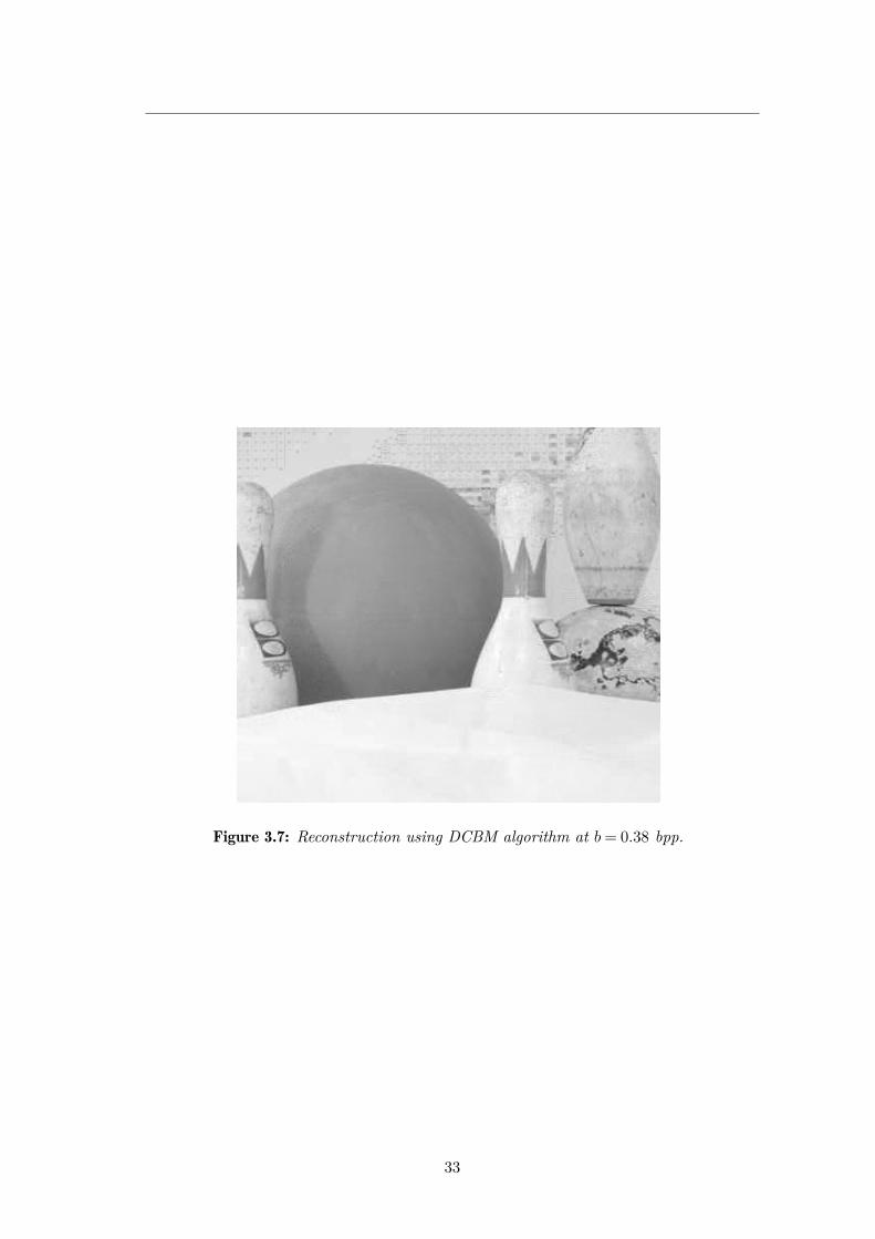
Figure 3.7: Reconstruction using DCBM algorithm at b= 0.38 bpp.

33


34

4

Ch

ap

te

r

Fast disparity map estimation algorithm improvingstereoscopic image compression

Summary

In the previous chapter a proof of concept work has already shown that

selecting disparities according to the compensated view, instead of the

predicted view, yields increased rate-distortion performance. Due to its

limitations in numerical complexity, this chapter proposes an algorithm deriving from

the JPEG coder a disparity dependent analytic expression of the distortion induced by

the compensated view.

The rest of this chapter is organized as follows. In Section.4.1, we recall the optimization

problem.Then we describe the principles of the proposed algorithm in Section 4.2. In

Section 4.3 evaluates the performance of the proposed Fast DCBM (FDCBM) algorithm

given experimental results. Finally, some conclusions are drawn in Section 4.4. This

contribution has resulted in one publication in an international journal [50].

Chapter 4. Fast disparity map estimation algorithm improving stereoscopic imagecompression

4.1 Optimization problem

4.1.1 Basic concepts and notations

In this chapter we consider rectified stereoscopic images using the classical DCC scheme.

The left image is chosen as the reference view and the right one as the target.

We keep the concepts and notations presented in Section 3.1.1 and illustrated in Fig. 3.1.

4.1.2 Formulation of the optimization problem

The optimization problem is described in Section 3.1.2. Furthermore, the mean squared

error between (Il, Il) and (Ir, Ir), is used as the cost function to be minimized. More

specifically, the mean squared error of the k-block of an image I′ as compared to that of

an image I is:

Jk(I′,I

)= 1|B|

∑(∆i,∆j)∈B

(I′[ik + ∆ijk + ∆j

]− I

[ik + ∆ijk + ∆j

])2

, (4.1)

where (∆i,∆j) spans the block B, (ik, jk) design the coordinate of the upper left corner

of the k-block and | | indicates the size of a set.

4.2 Proposed FDCBM algorithm

Due to the interesting performance of the DCBM algorithm (see [51]), this section

proposes a Fast version of this algorithm called FDCBM algorithm. The novelty is

that disparity selection is no longer based on the computation of Ir with all its pixel

values. The underlying idea of the developed algorithm is first discussed and then an

explicit formula of the JPEG-codec distorsion is derived. Blocks of size 8×8 pixels are

considered knowing that an extension to a larger block size is possible.

4.2.1 FDCBM algorithm underlying idea

This section considers that the size of B is 8×8 and more specifically that the disparity-

related blocks are exactly the JPEG-related blocks.

Introduce first some new notations. Define R =DrCqr (R) the reconstructed residual

at the decoder, and Ik any matrix of size 8×8:

36

Rk (∆i, j) = R (ik + ∆i, jk + j)

Rk (∆i, j) = R (ik + ∆i, jk + j)

‖Ik‖2 = 1|B|∑

(∆i,j)∈B (Ik(∆i, j))2

(4.2)

So as to be consistent with notations defined in Secion. 3.1.1, indexes of these 8×8

matrices start from 0: ∆i,∆j ∈ 0, . . .7. Note that because of the above block-related

assumption, Rk can also be considered as the decoded-encoded 8×8 matrix Rk:

Rk =DrCqr (Rk) . (4.3)

Our main claim is that the relevant pixel values are those of Rk, and that Jk

measures the mean squared distortions yielded by the compression and decompression

of Rk:

Jk

(Ir,Ir

)= Jk

(Ip + R,Ip + R

)= Jk

(R,R

)= ‖DrCqr (Rk)−Rk‖2 . (4.4)

The first equality is obtained with Eqs. (3.5) and (3.6). The second equality uses

an additive invariance property derived from Eq. (4.1). The third equality is computed

using Eqs. (4.1), (4.2) and (4.3).

4.2.2 JPEG encoding modelling

This section is interested in what JPEG encoding causes distortions, namely the

quantization of the DCT components:

DrCqr (Rk) = IDCT [Qqr (DCT [Rk])] , (4.5)

where Qqr is the 8×8-JPEG-quantizier.

As DCT is an orthogonal transformation, it preserves the L2 norm:

‖DrCqr (Rk)−Rk‖2 = ‖DCT [DrCqr (Rk)]−DCT [Rk]‖2 . (4.6)

Combining Eqs. (4.5) and (4.6), a minimized formula of the mean squared distortions

37


is obtained:

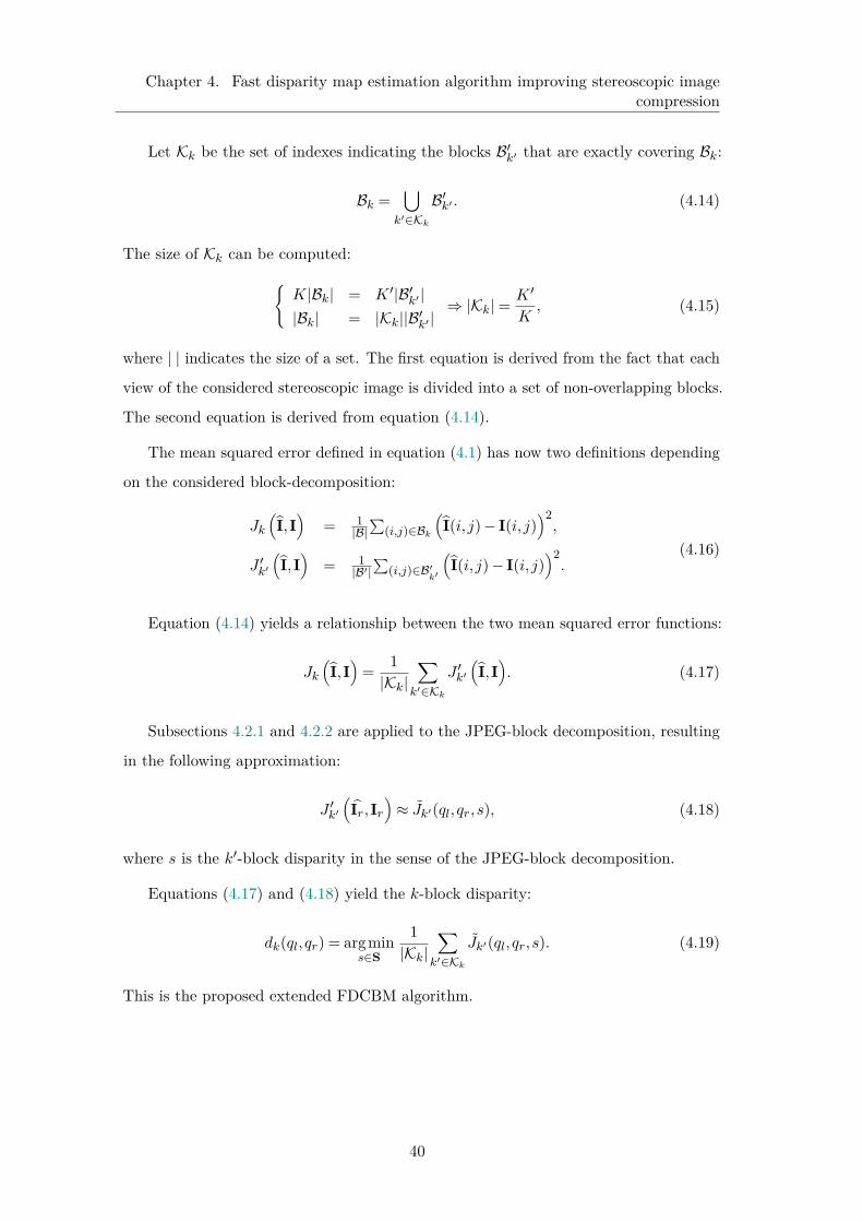
‖DrCqr (Rk)−Rk‖2 = ‖Qqr (DCT [Rk])−DCT [Rk]‖2 . (4.7)

The explicit formula uses the following information extracted from the JPEG codec

(see [52]). The DCT of an 8×8 matrix is:

DCT [Ik] = TT IkT, (4.8)

where T is an 8×8 orthogonal matrix defined as follows:

T∆i,j = 1√8

cos(π

(2j+ 1)∆i16

)×

1 if ∆i = 0√

2 if 1≤ ∆i≤ 7(4.9)

The JPEG quantization table is given by Eq. (2.5).

The JPEG quantizer transforms an 8×8 matrix into an 8×8 matrix:

Qqr (I) =[Round

( I(∆i, j)Q(∆i, j)α(qr)

)Q(∆i, j)α(qr)

]∆i,j

, (4.10)

using a nonlinear mapping transforms qr into a scaling factor (see [53]):

α(Q) =

50Q if Q≤ 502− Q

50 if Q> 50(4.11)

Experimentations have shown that Jk

(Ir,Ir

)is not exactly equal to the value of

‖Qqr (DCT [Rk])−DCT [Rk]‖2, and the latter depends on ql, qr and on the k block

disparity, s. So the following notation is used:

Jk (ql, qr,s) = ‖Qqr (DCT [Rk])−DCT [Rk]‖2 . (4.12)

Finally the k block disparity is selected as:

dk(ql, qr) = argmins∈S

Jk(ql, qr,s). (4.13)

4.2.3 Derived FDCBM algorithm

Instead of computing large scale images as with DCBM algorithm, only 8×8 matrices

are computed yielding to an approximation of Jk(Ir,Ir) (i.e. Jk(ql, qr,s)) using Eq.

(4.12). Moreover, instead of selecting the k-block disparity based on J(Ir,Ir), it is based

38

on the minimization of Jk(ql, qr,s). The numerical complexity of FDCBM algorithm

is then definitely much lower than that of DCBM algorithm. It remains higher than

the BM algorithm, not only because of the complexity of Eq. (4.12) but also because

it takes into account ql and qr, whereas BM takes into account only ql. The FDCBM

algorithm is summarized in Algorithm 3.

Algorithm 3 FDCBM algorithmInput: Il,Ir, ql, qr

Output: Cql(Il),C(d),Cqr (R), b,JCompute Cql(Il), Il with Eq. (3.1) and J(Il,Il) with Eqs. (4.1) and (3.8)for all k ∈ 1 . . .K do

for all s ∈ S doCompute Rk using Il and Ir with Eqs. (4.2), (3.2) and (3.5)Compute Jk(ql, qr,s) with Eq. (4.12)

end forSelect dk with Eq. (4.13) using all s-values of Jk(s)

end forCollect d = (d1, . . . ,dK) and compute C(d)Compute Ip with Eq. (3.2) using dCompute R = Ir − Ip and Cqr (R) with Eq. (3.5)Compute Ir with Eq. (3.6) and J(Ir,Ir) with Eq. (3.8)Compute J with Eq. (3.8) using J(Il,Il) and J(Ir,Ir)Compute b(Il,d,Ir, ql, qr) with Eq. (3.7) using Cql(Il),C(d),Cqr (R)

4.2.4 Extending the FDCBM algorithm to larger blocks

This section considers the case when the block decomposition yielding the disparity

map is not the same than the JPEG-block decomposition. To distinguish them, the

former is denoted Bk, (1≤ k ≤K, B as the set of internal displacements), the latter is

denoted B′k′ , (1≤ k′ ≤K ′, B′ as the set of internal displacements). In general, a block

Bk is likely to have common pixels with several blocks B′k′ and each of these blocks may

have common pixels with other blocks Bk′′ . In such a situation, the optimal choice of a

disparity dk depends on the choice of disparities of neighboring blocks, and adapting the

FDCBM algorithm seems difficult. Here we assume that each block Bk can be divided

exactly in a finite number of blocks B′k′ , and show how FDCBM can easily be extended.

For instance when an image is decomposed into 16×16-blocks, each of them covers

exactly four 8×8-blocks. And when an image is decomposed into 32×32-blocks, each of

them covers exactly sixteen 8×8-blocks.

39


Let Kk be the set of indexes indicating the blocks B′k′ that are exactly covering Bk:

Bk =⋃

k′∈Kk

B′k′ . (4.14)

The size of Kk can be computed:K|Bk| = K ′|B′k′ ||Bk| = |Kk||B′k′ |

⇒ |Kk|=K ′

K, (4.15)

where | | indicates the size of a set. The first equation is derived from the fact that each

view of the considered stereoscopic image is divided into a set of non-overlapping blocks.

The second equation is derived from equation (4.14).

The mean squared error defined in equation (4.1) has now two definitions depending

on the considered block-decomposition:

Jk

(I,I)

= 1|B|∑

(i,j)∈Bk

(I(i, j)− I(i, j)

)2,

J ′k′

(I,I)

= 1|B′|∑

(i,j)∈B′k′

(I(i, j)− I(i, j)

)2.

(4.16)

Equation (4.14) yields a relationship between the two mean squared error functions:

Jk

(I,I)

= 1|Kk|

∑k′∈Kk

J ′k′

(I,I). (4.17)

Subsections 4.2.1 and 4.2.2 are applied to the JPEG-block decomposition, resulting

in the following approximation:

J ′k′

(Ir,Ir

)≈ Jk′(ql, qr,s), (4.18)

where s is the k′-block disparity in the sense of the JPEG-block decomposition.

Equations (4.17) and (4.18) yield the k-block disparity:

dk(ql, qr) = argmins∈S

1|Kk|

∑k′∈Kk

Jk′(ql, qr,s). (4.19)

This is the proposed extended FDCBM algorithm.

40

4.3 Performance of the proposed algorithm

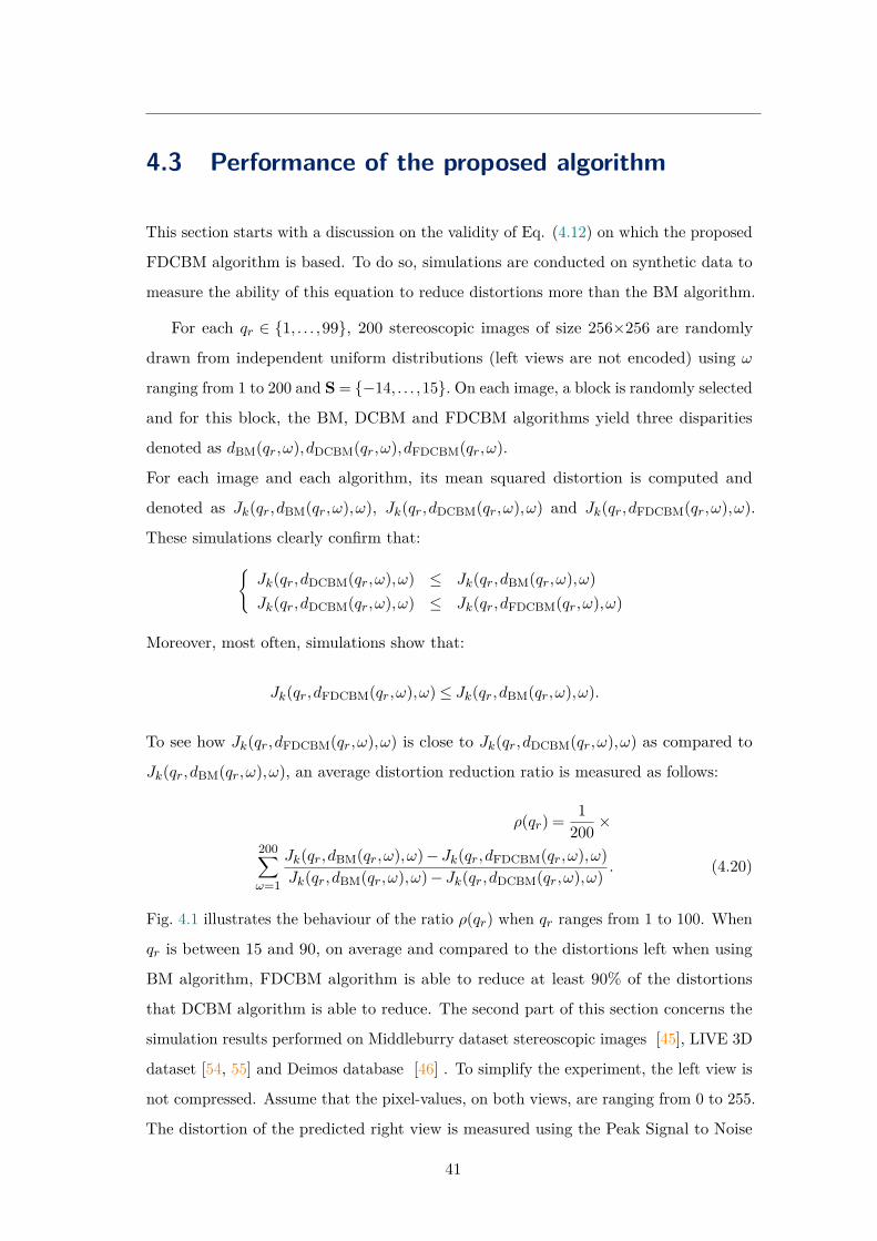
This section starts with a discussion on the validity of Eq. (4.12) on which the proposed

FDCBM algorithm is based. To do so, simulations are conducted on synthetic data to

measure the ability of this equation to reduce distortions more than the BM algorithm.

For each qr ∈ 1, . . . ,99, 200 stereoscopic images of size 256×256 are randomly

drawn from independent uniform distributions (left views are not encoded) using ω

ranging from 1 to 200 and S = −14, . . . ,15. On each image, a block is randomly selected

and for this block, the BM, DCBM and FDCBM algorithms yield three disparities

denoted as dBM(qr,ω),dDCBM(qr,ω),dFDCBM(qr,ω).

For each image and each algorithm, its mean squared distortion is computed and

denoted as Jk(qr,dBM(qr,ω),ω), Jk(qr,dDCBM(qr,ω),ω) and Jk(qr,dFDCBM(qr,ω),ω).

These simulations clearly confirm that:Jk(qr,dDCBM(qr,ω),ω) ≤ Jk(qr,dBM(qr,ω),ω)Jk(qr,dDCBM(qr,ω),ω) ≤ Jk(qr,dFDCBM(qr,ω),ω)

Moreover, most often, simulations show that:

Jk(qr,dFDCBM(qr,ω),ω)≤ Jk(qr,dBM(qr,ω),ω).

To see how Jk(qr,dFDCBM(qr,ω),ω) is close to Jk(qr,dDCBM(qr,ω),ω) as compared to

Jk(qr,dBM(qr,ω),ω), an average distortion reduction ratio is measured as follows:

ρ(qr) = 1200 ×

200∑ω=1

Jk(qr,dBM(qr,ω),ω)− Jk(qr,dFDCBM(qr,ω),ω)Jk(qr,dBM(qr,ω),ω)− Jk(qr,dDCBM(qr,ω),ω) . (4.20)

Fig. 4.1 illustrates the behaviour of the ratio ρ(qr) when qr ranges from 1 to 100. When

qr is between 15 and 90, on average and compared to the distortions left when using

BM algorithm, FDCBM algorithm is able to reduce at least 90% of the distortions

that DCBM algorithm is able to reduce. The second part of this section concerns the

simulation results performed on Middleburry dataset stereoscopic images [45], LIVE 3D

dataset [54, 55] and Deimos database [46] . To simplify the experiment, the left view is

not compressed. Assume that the pixel-values, on both views, are ranging from 0 to 255.

The distortion of the predicted right view is measured using the Peak Signal to Noise

41


Figure 4.1: Average distortion reduction ratio of BM-FDCBM compared to BM-DCBMon synthetic data (function of qr).

Ratio (PSNR) given by PSNR = 10log10

(2552

J(Ir,Ir)

)) and the Structural Similarity

Index (SSIM) [47]. The rate, in bits per pixel (bpp), is measured only on the right

view according to b= |C(d)|+|Cqr (R)||Ir| . The lossless coder, C is here an arithmetic coder

(see [48]). To reduce the numerical complexity, the set of quality factor values is reduced

to Qr = 5,10,15, . . . ,90. The set of all available disparities is S = 0, . . . ,120.

The rate-distortion curves, provided in Fig. 4.2, confirm the results stated above

using "Art" stereoscopic image of Middlebury-dataset (2005) and blocks of size 8×8.

Indeed the performance (in terms of rate-distortion) of the proposed FDCBM algorithm

is similar to that of DBCM algorithm, which is however better than that of the classical

BM algorithm and the Reference-based block matching algorithm called (R algorithm)

proposed in [1]. Corresponding SSIM values when using FDCBM algorithm are given

in Table 4.1 .

Fig. 4.3 presents the decompressed right image "Aloe" extracted from Middleburry

dataset (2006) using BM algorithm on the left side, R algorithm in the middle and

FDCBM on the right side. For each algorithm, blocks are of sizes 8×8 and qr ∈Qr is set

so that b= 0.3bpp. When comparing both reconstructed views with the original view, it

appears that the background cloth on right neighborhoods of each vertical leaf is wrongly

drawn. The reason may be that these neighborhoods are occluded in the left view. The

BM and R algorithms yield a dotted structure whereas the FDCBM algorithm yields a

slightly blurred square texture. From a PSNR-viewpoint, the FDCBM-reconstructed

view is closer to the original view (30.14dB) than the BM-reconstructed view (29.5dB)

42

Figure 4.2: Performance comparison of BM, DCBM, FDCBM and R algorithms using"Art" stereoscopic image of Middlebury-dataset (2005).

Table 4.1: SSIM values using FDCBM algorithm using "Art" stereoscopic image.

Bitrate SSIM0.25 0.670.27 0.840.29 0.880.32 0.890.35 0.910.37 0.910.4 0.920.42 0.930.44 0.930.47 0.940.49 0.940.52 0.950.56 0.950.61 0.950.67 0.960.77 0.960.92 0.971.19 0.97

and the R-reconstructed image (29.6dB).

43


Figure 4.3: Reconstructed "Aloe" right view: BM algorithm (left side); R algorithm(middle) and FDCBM algorithm (right side).

Fig. 4.4 shows the histograms of, on the left side, the BM-disparity map on the mid

side the R-disparity map, and on the right side, the FDCBM-disparity map for the same

experiment. More specifically, selected disparity values are sorted into 10 bins, each bin

is referred to by its average disparity value on the horizontal axis. The vertical axis

indicates the number of blocks for which the disparity value falls into a given bin (the

total number of blocks for that image is 2726). All histograms are right skewed, showing

that for most blocks it did not proved useful to consider disparity values greater than

50. A closer look shows that, on the right hand side, the two first columns are slightly

bigger and the two following columns are slightly smaller. This means that for this

specific image, on average FDCBM algorithm tends to select smaller disparity values

than BM and R algorithms.

Figure 4.4: Histogram of the disparity map yielded at b= 0.3bpp using "Aloe"stereoscopic image: BM algorithm (left side), R algorithm (on the middle) and FDCBM

algorithm (right side).

Fig. 4.5 provides the reconstructions of the "Dwarves" right view from Middleburry-

dataset 2005 using BM (in the left), R (on the middle) and FDCBM (on the right)

algorithms. A zoom on the vase (bottom right), shows that FDCBM gives much closer

reconstruction to the original view.

44

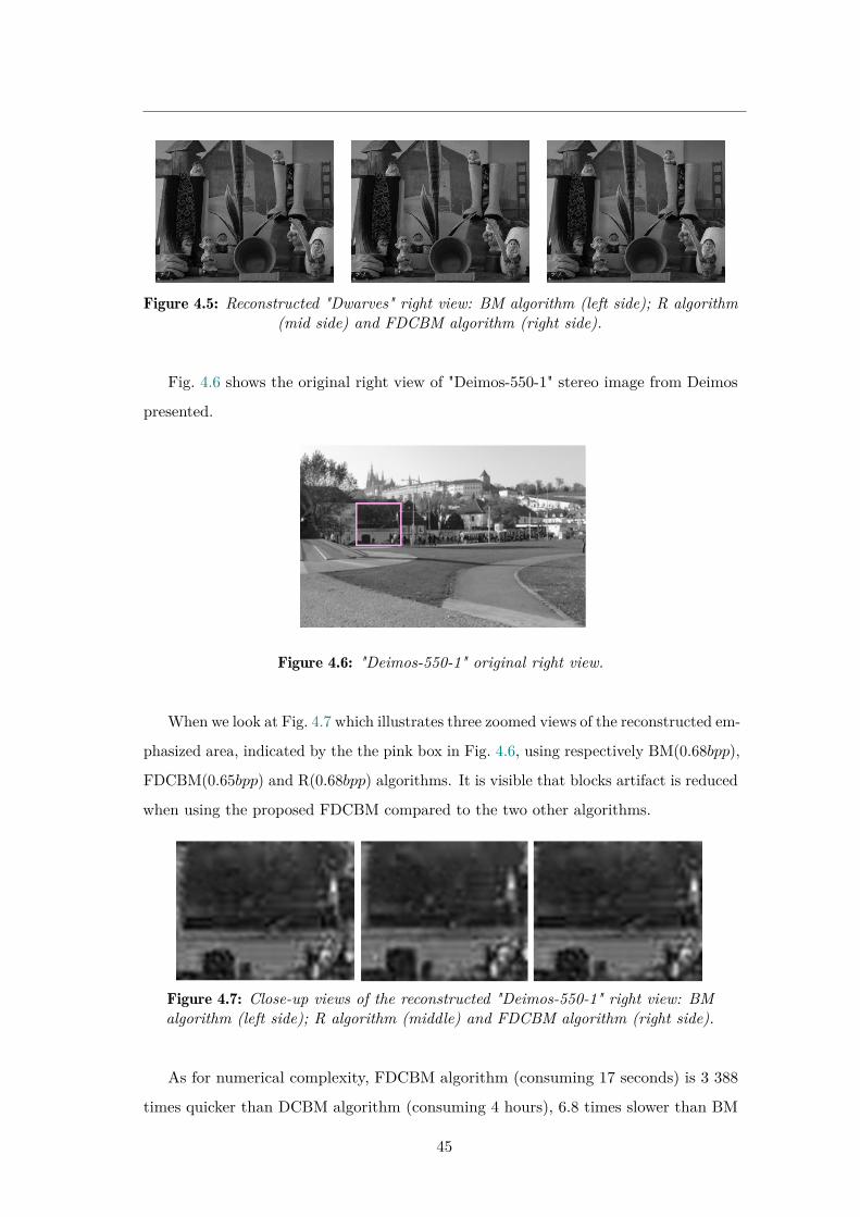
Figure 4.5: Reconstructed "Dwarves" right view: BM algorithm (left side); R algorithm(mid side) and FDCBM algorithm (right side).

Fig. 4.6 shows the original right view of "Deimos-550-1" stereo image from Deimos

presented.

Figure 4.6: "Deimos-550-1" original right view.

When we look at Fig. 4.7 which illustrates three zoomed views of the reconstructed em-

phasized area, indicated by the the pink box in Fig. 4.6, using respectively BM(0.68bpp),

FDCBM(0.65bpp) and R(0.68bpp) algorithms. It is visible that blocks artifact is reduced

when using the proposed FDCBM compared to the two other algorithms.

Figure 4.7: Close-up views of the reconstructed "Deimos-550-1" right view: BMalgorithm (left side); R algorithm (middle) and FDCBM algorithm (right side).

As for numerical complexity, FDCBM algorithm (consuming 17 seconds) is 3 388

times quicker than DCBM algorithm (consuming 4 hours), 6.8 times slower than BM

45


algorithm (consuming 2.5 seconds) and 1.5 times slower than R algorithm (consuming

12 seconds). This has been measured on the "Aloe" stereoscopic image with block of

8× 8 size using Matlab in a Windows environment on a computer using one processor

with four cores at a frequency of 3.7GHz.

The Bjøntegaard metric [49] is used here to quantify the increase in performance

of FDCBM algorithm as compared to BM and R algorithms. Based on four rate-

distortion points for each algorithm (roughly [0.3,0.4,0.5,0.6]bpp), it computes, an

average PSNR increase, or, an average bitrate decrease. As for the "Art" stereoscopic

image, FDCBM algorithm yields on average a PSNR increase of respectively 0.78dB and

0.52dB compared to the BM and R algorithms. To simplify its reading, the stereoscopic

images have been sorted by their increase in PSNR-performance to compare FDCBM

with BM algorithms.

Table 4.2 shows on columns 2 and 3 that, on average, for all stereoscopic images,

FDCBM is better performing than BM, the difference ranges from 0.42dB up to 1.69dB.

It seems difficult to understand why this difference is higher for some images and lower

on other images. For instance "Cloth3" and "Cloth4" appear at both ends of the table

and yet have similar appearance. The same comment applies to "Baby1" and "Baby3".

And both "Midd1", "Midd2" and "Lampshade1", "Lampshade2" have similar appearance

and yet each pair has quite different performance increases. It is interesting to note

that the stereoscopic image having the least PSNR-performance increase (+0.17dB),

namely "Plastic", is having a rather important bitrate decrease (−15.73%). Columns

4 and 5 of Table 4.2 summarizes the performance of our proposal compared to the R

algorithm. One can observe that the FDCBM algorithm achieves better performance

compared to the R algorithm. Table 4.3 provides other simulation results performed on

LIVE 3D database [54, 55].

The increase in performance of all stereoscopic images of FDCBM as compared to BM

is also shown in Fig. 4.8. More specifically, 10 bins have been considered ranging from

+0.25dB up to +1.25dB in terms of increase in terms of PSNR performance of FDCBM

as compared to BM. Each bar is associated to a specific bin, and its height indicates the

number of stereoscopic images, having an increase in PSNR performance of roughly the

amount indicated on the bin. The average increase in PSNR performance is 0.54dB.

46

Figure 4.8: Histogram of the increase in average PSNR-performance of FDCBM ascompared to BM, in terms of the number of stereoscopic images among the 30 extracted

from the 2005 and 2006 Middlebury-database.

4.4 ConclusionThis chapter presents a new block-based disparity estimation technique called FDCBM

algorithm. The purpose of this work is not to be competitive with stereoscopic im-

age\video standards, but to first show the feasibility of the proposed approach as a

proof of the concept. Where the classical technique selects each disparity so that the

predicted image resembles most to the right view, the proposed technique computes for

each disparity the compensated image, and the selected disparity is the one yielding the

highest similarity between the compensated image and the right view. The computation

is done with an analytic expression derived here from the JPEG-codec. To reduce

the numerical complexity, these computations are fed using only the considered block

pixel-values.

FDCBM algorithm is performing better than the classical Disparity Compensated Com-

pression scheme using a Block Matching and Reference based block matching disparity

estimation technique. To improve the performance of such proposal we can jointly

consider the bitrate and distortion to estimate the disparity. This will be discussed in

the next chapter.

47


Table 4.2: Performance comparison between FDCBM, BM and R algorithms usingBjøntegaard metric on Middlebury-datasets (2005-2006).

FDCBM versus BM algorithms FDCBM versus R algorithmsImage ∆PSNR (dB) bpp (%) ∆PSNR (dB) bpp (%)Plastic +0.17 -15,73 +0.41 -10,3Cloth3 +0.31 -7,44 +0.74 -12,78Midd1 +0.31 -4,79 +0.1 -6,5Cloth1 +0.34 -9,08 +0.2 -8.11Laundry +0.37 -5.66 +0.48 -7.61Computer +0.39 -6.3 +0.35 -6.09Baby1 +0.39 -8.17 +0.42 -10.03Baby2 +0.42 -9.35 +0.4 -7.44Wood1 +0.43 -8.9 +0.68 -17.64Rocks2 +0.44 -9.89 +0.49 -13.83Books +0.46 -7.93 +0.37 -5.61Aloe +0.53 -11.7 +0.6 -14.2Lampshade1 +0.54 -5.09 +0.66 -13.01Rocks1 +0.56 -12.43 +0.5 -13.53Bowling2 +0.57 -9.86 +0.77 -13.94Midd2 +0.58 -10.51 +0.11 -3.82Drumsticks +0.58 -8.85 +0.41 -6.67Dolls +0.59 -10.65 +0.51 -10.51Moebius +0.65 -11.44 +1.24 -22.59Cloth2 +0.66 -12.68 +0.73 -15.47Baby3 +0.67 -12.74 +0.55 -10.55Wood2 +0.72 -9.34 +0.65 -8.42Monopoly +0.75 -13.56 +0.44 -6.53Cloth4 +0.76 -17.12 +0.8 -14.63Art +0.78 -11.36 +0.52 -8.81Bowling1 +0.89 -14.47 +0.11 -20.98Dwarves +1.06 -17.48 +0.64 -12.64Flowerpots +1.12 -14.52 +1.12 -16.52Lampshade2 +1.23 -22.76 +0.91 -18.23Mean +0.62 -11.38 +0.54 -11.62

48

Table 4.3: Performance comparison between FDCBM, BM and R algorithms using theBjøntegaard metric on 3D LIVE-database.

FDCBM versus BM algorithms FDCBM versus R algorithmsImage ∆PSNR (dB) bpp (%) ∆PSNR (dB) bpp (%)im8 +0.21 -5.85 +0.3 -1,76im29 +0.22 -7.06 +0.15 -5.13im13 +0.25 -7.43 +0.13 -4.03im18 +0.34 -7.52 +0.15 -3.64im3 +0.36 -11.14 +0.23 -7.68im17 +0.51 -17.75 +0.4 -13.96im10 +0.55 -14.22 +1.46 -8.5im26 +0.61 -17.23 +0.51 -19.27im5 +0.62 -18.26 +0.39 -11.34Mean +0.42 -12.74 +0.23 -8.37

49


50

5

Ch

ap

te

r

Disparity estimation using a joint bitrate-distortionmetric in the compensation coding scheme

Summary

C hallenging the exploitation of stereoscopic image redundancy to increase

compression bitrate-distortion performance. In this chapter, an algorithm

combining two existing compression algorithms is presented. These latter

are different, one is performing better at low- and mid-range bitrates, it is the R-

algorithm [1], the other at mid- and high-range bitrates, it is the FDCBM presented in

the previous chapter. One iteratively modifies the disparity map to improve the bitrate-

distortion trade-off using a Lagrangian multiplier. The other selects each disparity on a

block basis, according to a simplified model of how JPEG deals with the compensation

refinement. The remainder of this chapter is organized as follows. Section 5.1 recalls

some notations and concepts related to the BM and FDCBM algorithms. Section 5.2

describes the R algorithm. Section 5.3 provides a description of the developed algorithm.

In section 5.4, simulation results evaluating the proposed algorithm’s performance is

given. Finally, section 5.5 concludes this chapter. The main contribution, provided in

this chapter, have been submitted to the international conference [56].

Chapter 5. Disparity estimation using a joint bitrate-distortion metric in thecompensation coding scheme

5.1 Notations and formulations

Let us recall some notations and formulations related to the BM and FDCBM [50]

algorithms.

When a disparity map, of K blocks, d = (d0, . . . ,dK−1) is estimated using the BM

algorithm, each component dk (k ∈ 0, . . . ,K) is selected so that the kth-block in the

left view, is horizontally shifted by dk, and best matches the kth-block in the right view,

in terms of mean square error Dk:

Dk(ql,s) =∑

(∆i,∆j)∈B

(Il

[ik +∆i

jk +∆j+ s

]− Ir

[ik +∆ijk +∆j

])2

, (5.1)

where s is a disparity value taken from the search window S, (∆i,∆j) spans the block B,

(ik, jk) design the coordinate of the upper left corner of the kth-block, s is a disparity

value, Ir is the right view and Il is the decoded left image using the ql parameter.

The disparity dk, estimated using the BM algorithm, is then selected as:

d(BM)k = argmin

s∈SDk(ql,s). (5.2)

As described in Section. 4.2, FDCBM algorithm overlooks the cost of storing the

disparity map and selects the blockwise disparity taking into account the compensation

refinement assuming that JPEG is used for compensation. The modeled compensation

aware distortion is:

Dk(ql, qr,s) = ‖Qqr (DCT [Rk])−DCT [Rk]‖2 , (5.3)

where ||.||2 is the L2 norm, Rk designs the k- block of the residual error R, Qqr is the

8× 8 JPEG quantizer, ql and qr are hyperparameters used respectively for coding the

left view and the residual error and s is a disparity value taken for the kth block.

The k-block disparity using FDCBM algorithm is given by:

d(FDCBM)k = argmin

s∈SDk(ql, qr,s). (5.4)

Note that the use of D in these formulas instead of J in previous chapters is to design

distortion.

52

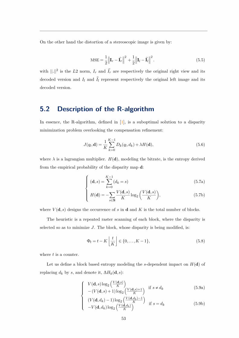
On the other hand the distortion of a stereoscopic image is given by:

MSE = 12∥∥∥Ir − Ir

∥∥∥2+ 1

2∥∥∥Il− Il

∥∥∥2. (5.5)

with ||.||2 is the L2 norm, Ir and Ir are respectively the original right view and its

decoded version and Il and Il represent respectively the original left image and its

decoded version.

5.2 Description of the R-algorithm

In essence, the R-algorithm, defined in [1], is a suboptimal solution to a disparity

minimization problem overlooking the compensation refinement:

J(ql,d) = 1K

K−1∑k=0

Dk(ql,dk) +λH(d), (5.6)

where λ is a lagrangian multiplier. H(d), modeling the bitrate, is the entropy derived

from the empirical probability of the disparity map d:(d,s) =

K−1∑k=0

(dk = s) (5.7a)

H(d) =−∑s∈S

V (d,s)K

log2

(V (d,s)K

), (5.7b)

where V (d,s) designs the occurrence of s in d and K is the total number of blocks.

The heuristic is a repeated raster scanning of each block, where the disparity is

selected so as to minimize J . The block, whose disparity is being modified, is:

Φt = t−K⌊t

K

⌋∈ 0, . . . ,K − 1, (5.8)

where t is a counter.

Let us define a block based entropy modeling the s-dependent impact on H(d) of

replacing dk by s, and denote it, ∆Hk(d,s):

V (d,s) log2(

V (d,s)K

)−(V (d,s) + 1)log2

(V (d,s)+1

K

) if s , dk (5.9a)

(V (d,dk)− 1) log2(

V (d,dk)−1K

)−V (d,dk) log2

(V (d,dk)

K

) if s= dk (5.9b)

53


As mentioned in [1], considering two disparity maps d and d′ whose only difference

is that d′k = s and dk = dk, we have:

H(d′) =H(d) +∆Hk(d,s)−(V (d,dk)− 1) log2

(V (d,dk)−1

K

)+V (d,dk) log2

(V (d,dk)

K

).

(5.10)

Note that equations (5.1) and (5.10) show that minimizing J with respect to dk is

equivalent to minimizing Dk(ql,s) +λ∆Hk(d,s).

The recast equations of the R-algorithm are:

d0 = d(BM),

dt+1k =

argmins∈S

DΦt(ql,s) +λ∆HΦt

(dt,s) if k = Φt

dtk if k , Φt,

(5.11)

where t is increased as long as t ≤ K and dt , dt−1. The yielded disparity map is

denoted as d(R), which depends on ql and λ.

5.3 Proposed COMB-algorithm

Thanks to the new notations, combining the R and FDCBM algorithms is now straight-

forward, and our proposal is:

d0 = d(FDCBM),

dt+1k =

argmins∈S

DΦt(ql, qr,s) +λ∆HΦt

(dt,s) if k = Φt

dtk if k , Φt

(5.12)

where t is increased as long as t ≤ K and dt , dt−1. The resulted disparity map is

denoted as d(COMB).

The only differences between the COMB-algorithm and R-algorithm is the choice

of the initial disparity, the 8×8 block size and the use of Dk instead of Dk. Note that

since dt depends on ql, qr and λ, ∆HΦt(dt,s) depends also on these parameters.

The COMB-algorithm is described below (see Algorithm 4).

54

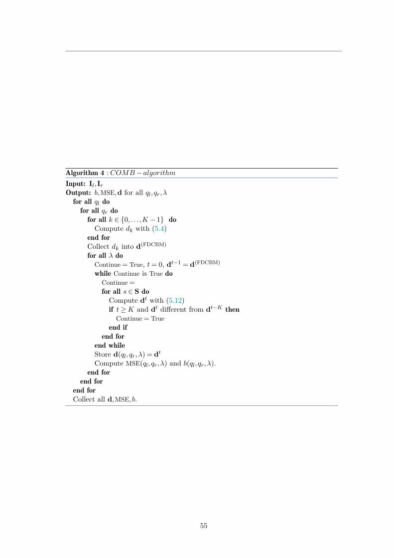
Algorithm 4 : COMB− algorithmInput: Il,Ir

Output: b,MSE,d for all ql, qr,λfor all ql do

for all qr dofor all k ∈ 0, . . . ,K − 1 doCompute dk with (5.4)

end forCollect dk into d(FDCBM)

for all λ doContinue = True, t= 0, dt−1 = d(FDCBM)

while Continue is True doContinue =for all s ∈ S doCompute dt with (5.12)if t≥K and dt different from dt−K then

Continue = Trueend if

end forend whileStore d(ql, qr,λ) = dt

Compute MSE(ql, qr,λ) and b(ql, qr,λ).end for

end forend forCollect all d,MSE, b.

55


5.4 Experiments and results

The BM, R, FDCBM and COMB algorithms have been tested on a set of stereoscopic

images. This section provides the results using "Monopoly" stereoscopic image extracted

from the 2006-Middleburry dataset [45] and "Ballon" stereoscopic image extracted from

the MCL-3D dataset [57].

For the sake of simplicity, the left view is not coded. The bitrate is deduced as follows:

b= |C(d)|+|Cqr (R)||Ir| . The lossless compression of the disparity map is implemented using

an entropy coder and JPEG is used to code the residual. The distortion is accounted

for by MSE =∥∥∥Ir − Ir

∥∥∥2.The PSNR and SSIM compare Ir with Ir.

Fig. 5.1 presents the rate-distortion curves obtained when compressing "Monopoly"

using the four algorithms. The BM-curve in green is below with the R-curve in magenta

slightly above it. Clearly above at high bitrate and below at low bitrate is the FDCBM-

curve in blue. Above all these curves is the COMB-curve. What is striking, is that,

even though by themselves, the R- and FDCBM algorithms are not doing that well, the

COMB algorithm is significantly above at low- and mid-range bitrates.

Much the same can be said of Fig. 5.2 which is the rate-distortion curve obtained

when compressing "Ballon". The increase in performance may seem quite surprising

as the R-curve and the BM-curve are hardly distinguishable. The FDCBM algorithm

has very low performance at low bitrate. And yet the COMB algorithm has still

significant increase in compressing performance compare to the BM algorithm at low-

and mid-range bitrates.

Fig. 5.4 provides the histograms of the disparity maps yielded by the four different

algorithms when compressing "Monopoly" at b= 0.33. The cost of storing the disparity

map is modeled with the entropy which is computed using such disparity histograms.

Basically the more a disparity map has most of its values included in a small set of

values, the lower is the entropy. With no surprise, histograms obtained with the R and

COMB algorithms have much lower entropy as compared to those obtained with the

BM and FDCBM algorithms.

The original right view of "Monopoly" stereoscopic image is depicted in Fig. 5.3.

Fig. 5.5 shows the right view reconstruction at b = 0.33bpp when compression is

achieved with the BM algorithm. On a computer screen with some zooming, white thin

56

Figure 5.1: Performance comparison of BM, R, FDCBM and COMB algorithms on the"Monopoly" stereoscopic image .

57


Figure 5.2: Performance comparison of BM, R, FDCBM and COMB algorithms using"Ballon" stereoscopic image.

58

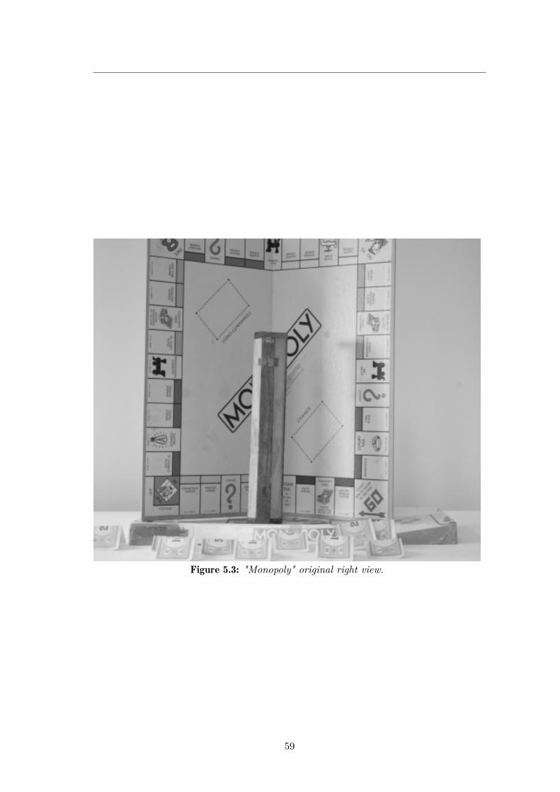
Figure 5.3: "Monopoly" original right view.

59


vertical lines can be seen both at the right of the vertical thin piece of wood and at

the right of the "Monopoly" board. These vertical lines are slightly less visible when

compression is achieved with the R algorithm. However when compression is achieved

with the FDCBM algorithm these white lines are hardly visible, they are replaced by

gray squares of equal size and randomly padding the left, the right and the interior of

the "Monopoly" board, such squares may be a little more visible than the vertical white

lines. When compression is achieved with the COMB algorithm, the white lines remain

hardly visible but the gray squares have also vanished assessing here an improvement.

BM R

FDCBM COMBFigure 5.4: Histogram of the disparity map yielded at b= 0.33 bpp using Monopoly.

5.5 Conclusion

This chapter presented a new stereo-matching algorithm jointly optimizing the bitrate

and the distortion. The proposed algorithm, called COMB-algorithm, combines the de-

veloped FDCBM algorithm and the Reference based block matching disparity estimation

60

Figure 5.5: Reconstructed right view with the BM algorithm, (PSNR = 35.28dB,SSIM = 0.95, b= 0.33bpp).

61


Figure 5.6: Reconstructed right view with the R algorithm (PSNR = 35.89dB,SSIM = 0.95, b= 0.33bpp).

62

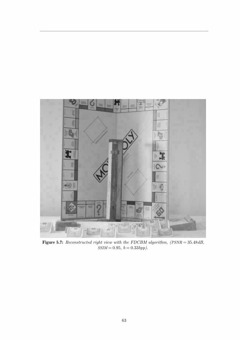
Figure 5.7: Reconstructed right view with the FDCBM algorithm, (PSNR = 35.48dB,SSIM = 0.95, b= 0.33bpp).

63


Figure 5.8: Reconstructed right view with the COMB algorithm, (PSNR = 36.58dB,SSIM = 0.97, b= 0.33bpp).

64

algorithm. Simulation results shown that it seems that this important difference between

the two algorithms explain the interesting performances observed. An important study

is investigated to understand, when and why, performances are significantly improved

using some indicators based on spatial and disparity information.

65


66

6

Ch

ap

te

r

Conclusion and Perspectives

Over the few last years, 3D imaging systems have been widely spread in numerous

applications such as entertainment, industry, medical domains, cartography,... Stereo-

scopic technologies require the use of a pair of image representing the same scene from

two different angles. This means that the amount of data needed for transmission and

storage purposes is twice compared to that induced by a single image.

In order to exploit view redundancies, efficient compression techniques should be em-

ployed. The work carried out in this document falls within this context and this research

work has been dedicated. To improve the Disparity Compensated Compression scheme,

we are focused precisely on the disparity map estimation. This latter is very important

because it impacts the performance in terms of rate distortion. In the following, we

provide the main contributions we have made to this issue and mention some possible

future perspectives.

The first contribution of this PhD thesis was the development of Disparity Compen-

sated Block Matching (DCBM) algorithm showing that the proposed strategy gives

better results in terms of rate distortion compared to the classical methods adopted by

most image /video standards. In the proposed strategy, the blockwise disparity map

is estimated taking into account the compensation effect. In the classical Disparity

Compensated Compression (DCC) scheme, when using the Block Matching algorithm,

a disparity map is estimated to predict the right image the most similar to its original

version. Then the residual error, as the difference between the original view and its

Chapter 6. Conclusion and Perspectives

prediction, is encoded yielding a refinement (i.e compensation) added to the predicted

image. The DCBM algorithm operates differently. It improves first all the possible

predicted images considering this refinement. Then the selected disparity map is the

one with which the predicted view is most similar to that same original view. This

shows a proof of the disparity map estimation concept controlled by the compensated

view instead of the predicted one before compensation. Despite its efficiency compared

to BM and R algorithms, the proposed DCBM algorithm has the drawback that it

increases the numerical complexity. This is because of the necessity to code and decode

a new residual error each time a new disparity value is considered. A possible way to

make this algorithm faster is the including of parallel programming.

The second contribution of this dissertation was concerned to find a solution to the

computational complexity problem of the DCBM algorithm. The proposed algorithm,

called FDCBM (FastDCBM) algorithm, estimates the disparity map by a simplified

modelling of how the coding of the residual error copes with the compensation. At this

end, an analytic expression is derived based on the quantization of the DCT coefficients,

cause of the distortion, in the JPEG coder. To select disparity, only 8× 8 blocks of the

residual error are used not the whole error with all its pixels. That is why the numerical

complexity was significantly decreased compared to the previous DCBM-algorithm.

The proposed FDCBM-algorithm performs better than the DCC using BM and R

algorithms. This former could be integrated in the stereoscopic image/video coding to

further improve the performance when using the DCC scheme.

The performance of the proposed DCBM and FDCBM algorithms can be improved in

two ways: First, homologous blocks do not necessarily belongs to the same scan line.

Hence disparities have an horizontal and vertical components. Second, search window

can take real values. This gives more precision for the matching task.

The last contribution of this work focused on estimating disparity map given the best

compromise between the minimization of the distortion of the predicted view and

the bitrate allocated to encode the disparity map. The proposed algorithm, called

COMB-algorithm, combines two algorithms: the R-algorithm performing better at at

low bitrates and the developed FDCBM one more efficient at high bitrates.

An important area of research will consist in the interpretation of the behaviour of the

COMB algorithm at different bitrate ranges. Inspired from the TI (disparity informa-

tion) and SI (spatial information) for characterizing the stereoscopic image as for video

68

sequence [58], it will be interesting to use this information to understand the relation

between the nature of stereoscopic image and how our proposed COMB-algorithm

behaves. Moreover, spatial and temporal information can be used with others features

such as the variance, mean ,. . . of stereoscopic image as attribute for a technique of

machine learning in order to categorize such image. Another perspective work may

consider to extend the developed algorithms to stereoscopic videos. Last but not least,

further investigations deserve to be conducted concerning the use the principle of our

proposed methods with the motion compensation scheme.

69

Chapter 6. Conclusion and Perspectives

70

Bibliography

[1] Aysha Kadaikar, Gabriel Dauphin, and Anissa Mokraoui. “Modified block matchingalgorithm improving rate-distortion performance for stereoscopic image coding”.In: 2015 IEEE International Symposium on Signal Processing and InformationTechnology (ISSPIT). Dec. 2015, pp. 478–483. doi: 10 . 1109 / ISSPIT . 2015 .

7394383 Cited on pages 3, 18, 28, 42, 51, 53, 54.

[2] url: https://www.vision3d.com/stereo.html. Cited on page 8.

[3] url: http://camera-wiki.org/wiki/Stereo. Cited on page 8.

[4] Olivier Faugeras. Three-Dimensional Computer Vision: A Geometric Viewpoint.Cambridge, MA, USA: MIT Press, 1993 Cited on page 9.

[5] F. Dufaux, B. Pesquet-Popescu, and M. Cagnazzo. Emerging Technologies for3D Video: Creation, Coding, Transmission and Rendering. 1st. Wiley Publishing,2013. isbn: 1118355113, 9781118355114 Cited on pages 10–12, 15, 16.

[6] Zhengyou Zhang and Gang Xu. “A General Expression of the Fundamental Matrixfor Both Perspective and Affine Cameras”. In: 2 (Nov. 1997) Cited on page 10.

[7] Zhengyou Zhang. “Determining the Epipolar Geometry and its Uncertainty: AReview”. In: International Journal of Computer Vision 27 (1998), pp. 161–195Cited on page 10.

[8] Andrea Fusiello, Emanuele Trucco, and Alessandro Verri. “A Compact Algorithmfor Rectification of Stereo Pairs”. In: Mach. Vision Appl. 12.1 (July 2000), pp. 16–22 Cited on page 10.

[9] Richard Hartley and et al. “Computing matched-epipolar projections”. In: Pro-ceedings of IEEE Conference on Computer Vision and Pattern Recognition. June1993, pp. 549–555. doi: 10.1109/CVPR.1993.341076 Cited on page 10.

[10] Rong Pan, Zheng-Xin Hou, and Yu Liu. “Fast Algorithms for Inter-view Predictionof Multiview Video Coding”. In: Journal of Multimedia 6 (2011), pp. 191–201Cited on page 10.

[11] Ohta and Takeo Kanade. “Stereo by Intra- and Inter-Scanline Search UsingDynamic Programming”. In: IEEE Transactions on Pattern Analysis and MachineIntelligence PAMI-7.2 (Mar. 1985), pp. 139–154. doi: 10.1109/TPAMI.1985.

4767639 Cited on page 11.

https://doi.org/10.1109/ISSPIT.2015.7394383


https://www.vision3d.com/stereo.html.

http://camera-wiki.org/wiki/Stereo.

https://doi.org/10.1109/CVPR.1993.341076

https://doi.org/10.1109/TPAMI.1985.4767639

https://doi.org/10.1109/TPAMI.1985.4767639

Bibliography

[12] Cordelia Schmid and Andrew Zisserman. “The Geometry and Matching of Linesand Curves Over Multiple Views”. In: International Journal of Computer Vision40 (Dec. 2000), pp. 199–233. doi: 10.1023/A:1008135310502 Cited on page 11.

[13] Gerard Medioni and Ramakant Nevatia. “Segment-based stereo matching”. In:Computer Vision, Graphics, and Image Processing 31.1 (1985), pp. 2–18. doi:https://doi.org/10.1016/S0734-189X(85)80073-6 Cited on page 11.

[14] Hexin Chen Xing Ma and Yan Zhao. “Stereo image coding method using stereomatching with difference-based adaptive searching windows”. In: 2009 IEEEInternational Workshop on Imaging Systems and Techniques. May 2009, pp. 373–376. doi: 10.1109/IST.2009.5071668 Cited on page 12.

[15] Olga Veksler. “Stereo matching by compact windows via minimum ratio cycle”. In:Proceedings Eighth IEEE International Conference on Computer Vision. ICCV2001. Vol. 1. July 2001, 540–547 vol.1. doi: 10.1109/ICCV.2001.937563 Cited onpage 12.

[16] Antonio Ortega Woontack Woo. “Overlapped block disparity compensation withadaptive windows for stereo image coding”. In: IEEE Transactions on Circuitsand Systems for Video Technology 10.2 (Mar. 2000), pp. 194–200. doi: 10.1109/

76.825718 Cited on page 12.

[17] Olga Veksler. “Stereo correspondence by dynamic programming on a tree”. In: 2005IEEE Computer Society Conference on Computer Vision and Pattern Recognition(CVPR’05). Vol. 2. June 2005, 384–390 vol. 2. doi: 10.1109/CVPR.2005.334

Cited on page 12.

[18] Jae Chul Kim et al. “A dense stereo matching using two-pass dynamic program-ming with generalized ground control points”. In: 2005 IEEE Computer SocietyConference on Computer Vision and Pattern Recognition (CVPR’05). Vol. 2. June2005, 1075–1082 vol. 2. doi: 10.1109/CVPR.2005.22 Cited on pages 12, 13.

[19] Sébastien Roy and Ingemar J. Cox. “A maximum-flow formulation of the N-camerastereo correspondence problem”. In: Sixth International Conference on ComputerVision (IEEE Cat. No.98CH36271). Jan. 1998, pp. 492–499. doi: 10.1109/ICCV.

1998.710763 Cited on page 13.

[20] Sergey Kosov, Thorsten Thormählen, and Hans-Peter Seidel. “Accurate Real-TimeDisparity Estimation with Variational Methods”. In: Nov. 2009, pp. 796–807. doi:10.1007/978-3-642-10331-5_74 Cited on page 13.

[21] Pedro F. Felzenszwalb and Daniel P. Huttenlocher. “Efficient belief propagationfor early vision”. In: Proceedings of the 2004 IEEE Computer Society Conferenceon Computer Vision and Pattern Recognition, 2004. CVPR 2004. Vol. 1. June2004. doi: 10.1109/CVPR.2004.1315041 Cited on page 13.

[22] Cassius C. Cutler. “Differential quantization of communication signals”. 2605361.July 1952 Cited on page 14.

72

https://doi.org/10.1023/A:1008135310502

https://doi.org/https://doi.org/10.1016/S0734-189X(85)80073-6

https://doi.org/10.1109/IST.2009.5071668

https://doi.org/10.1109/ICCV.2001.937563

https://doi.org/10.1109/76.825718

https://doi.org/10.1109/76.825718





https://doi.org/10.1007/978-3-642-10331-5_74


[23] Rao, Kamisetty Ramamohan, and Pat C Yip. Discrete Cosine Transform: Algo-rithms, Advantages, Applications. USA: Academic Press Professional, Inc., 1990Cited on page 14.

[24] Stephane Mallat. A Wavelet Tour of Signal Processing, Third Edition: The SparseWay. 3rd. USA: Academic Press, Inc., 2008 Cited on page 14.

[25] Gregory K. Wallace. “The JPEG Still Picture Compression Standard”. In: IEEETrans. on Consum. Electron. 38.1 (Feb. 1992), pp. xviii–xxxiv. doi: 10.1109/30.

125072 Cited on pages 14, 15.

[26] ITU-T Recommendation H.263: Video coding for low bit rate communication. 1998Cited on page 14.

[27] Thomas Wiegand et al. “Overview of the H.264/AVC video coding standard”.In: IEEE Trans. Circuits Syst. Video Techn. (2003). doi: 10.1109/TCSVT.2003.


[28] ITU-T Recommendation H.265: High efficiency video coding. 2019 Cited onpage 14.

[29] David Taubman and Michael Marcellin. JPEG2000 Image Compression Funda-mentals, Standards and Practice. Springer Publishing Company, Incorporated,2013 Cited on pages 14, 15.

[30] Anthony Vetro, Thomas Wiegand, and Gary J. Sullivan. “Overview of the Stereoand Multiview Video Coding Extensions of the H.264/MPEG-4 AVC Standard”.In: Proceedings of the IEEE 99.4 (2011), pp. 626–642. doi: 10.1109/JPROC.2010.


[31] T. Wiegand et al. “Overview of the H.264/AVC video coding standard”. In: IEEETransactions on Circuits and Systems for Video Technology 13.7 (July 2003),pp. 560–576. issn: 1558-2205. doi: 10.1109/TCSVT.2003.815165 Cited on page 16.

[32] Walid Hachicha. “Towards efficient methods for stereoscopic image processing,coding and quality assessment”. PhD thesis. Paris 13, 2014 Cited on page 17.

[33] A. Kadaikar, G. Dauphin, and A. Mokraoui. “Sequential Block-Based DisparityMap Estimation Algorithm for Stereoscopic Image Coding”. In: Elsevier journal,Signal Processing: Image Communication (2015). doi: 10.1016/j.image.2015.

09.007 Cited on page 18.

[34] Aysha Kadaikar, Gabriel Dauphin, and Anissa Mokraoui. “Extended map estima-tion algorithm using joint entropy-distortion metric for non-rectified stereoscopicimages”. In: IEEE International Symposium on Signal Processing and InformationTechnology, ISSPIT 2015, Abu Dhabi, United Arab Emirates, December 7-10, 2015.2015, pp. 505–510. doi: 10.1109/ISSPIT.2015.7394388 Cited on page 18.

73

https://doi.org/10.1109/30.125072

https://doi.org/10.1109/30.125072

https://doi.org/10.1109/TCSVT.2003.815165


https://doi.org/10.1109/JPROC.2010.2098830

https://doi.org/10.1109/JPROC.2010.2098830


https://doi.org/10.1016/j.image.2015.09.007



Bibliography

[35] Aysha Kadaikar, Gabriel Dauphin, and Anissa Mokraoui. “Joint Disparity andVariable Size-Block Optimization Algorithm for Stereoscopic Image Compression”.In: Elsevier journal, Signal Processing:Image Communication (2017). doi: 10.

1016/j.image.2017.10.008 Cited on page 18.

[36] Aysha Kadaikar, Gabriel Dauphin, and Anissa Mokraoui. “Improving block-matching algorithm by selecting disparity sets minimizing distortion for stereo-scopic image coding”. In: 6th European Workshop on Visual Information Process-ing, EUVIP 2016, Marseille, France, October 25-27, 2016. 2016, pp. 1–5. doi:10.1109/EUVIP.2016.7764593 Cited on page 18.

[37] Halûk Aydinoglu et al. “Region-based stereo image coding”. In: Proceedings.,International Conference on Image Processing. Vol. 2. Oct. 1995, 57–60 vol.2. doi:10.1109/ICIP.1995.537414 Cited on page 18.

[38] Michael G. Perkins. “Data compression of stereopairs”. In: IEEE Transactions onCommunications 40.4 (Apr. 1992), pp. 684–696. doi: 10.1109/26.141424 Citedon page 18.

[39] Qin Jiang, Joon Jae Lee, and M. H. Hayes. “A wavelet based stereo image codingalgorithm”. In: 1999 IEEE International Conference on Acoustics, Speech, andSignal Processing. Proceedings. ICASSP99 (Cat. No.99CH36258). Vol. 6. Mar.1999, 3157–3160 vol.6. doi: 10.1109/ICASSP.1999.757511 Cited on page 18.

[40] Aldo Maalouf and Mohamed-Chaker Larabi. “Bandelet-based stereo image cod-ing”. In: 2010 IEEE International Conference on Acoustics, Speech and SignalProcessing. Mar. 2010, pp. 698–701. doi: 10.1109/ICASSP.2010.5495084 Citedon page 18.

[41] Mounir Kaaniche et al. “Dense disparity map representations for stereo imagecoding”. In: IEEE International Conference on Image Processing. Egypt, Nov.2009, pp. 725–728 Cited on page 18.

[42] Imen Kadri et al. “Algorithme d’appariement de blocs basé sur l’optimisationde la compensation de disparité pour le codage d’image stéréoscopique”. In:Compression et Représentation des Signaux Audiovisuels (CORESA). 2018 Citedon page 21.

[43] Imen Kadri et al. “Stereoscopic Image Coding Performance using Disparity-Compensated Block Matching Algorithm”. In: Signal Processing: Algorithms,Architectures, Arrangements and Applications (SPA). 2019 Cited on page 21.

[44] Alexandre Benoit et al. “Using disparity for quality assessment of stereoscopicimages”. In: 15th IEEE International Conference on Image Processing. Nov. 2008,pp. 389–392 Cited on page 24.

[45] Daniel Scharstein and Chris Pal. “Learning Conditional Random Fields for Stereo”.In: IEEE Conference on Computer Vision and Pattern Recognition. 2007, pp. 1–8Cited on pages 28, 41, 56.

74



https://doi.org/10.1109/EUVIP.2016.7764593

https://doi.org/10.1109/ICIP.1995.537414

https://doi.org/10.1109/26.141424

https://doi.org/10.1109/ICASSP.1999.757511

https://doi.org/10.1109/ICASSP.2010.5495084

[46] Karel Fliegel et al. “Open source database of images DEIMOS: high dynamicrange images”. In: Proc. SPIE 7798 (2010), pp. 1016–1023 Cited on pages 28, 41.

[47] Zhou Wang et al. “Image quality assessment: from error visibility to structuralsimilarity”. In: IEEE Trans. Image Processing 13.4 (2004), pp. 600–612. doi:10.1109/TIP.2003.819861 Cited on pages 28, 42.

[48] Paul G. Howard and Jeffrey Vitter. “Arithmetic Coding for Data Compression”.In: Proceedings of the IEEE 82 (July 1994), pp. 857–865 Cited on pages 28, 42.

[49] Gisle Bjøntegaard. Calculation of average PSNR differences between RD-curves.Document VCEG-M33. ITU-T VCEG Meeting, Austin, Texas, USA, 2001, pp. 1–4Cited on pages 29, 46.

[50] Imen Kadri et al. “Disparities selection controlled by the compensated imagequality for a given bitrate”. In: Signal, Image and Video Processing (). Acceptedfor publication, p. 8. doi: 10.1007/s11760-020-01643-1 Cited on pages 35, 52.

[51] Imen Kadri et al. “Stereoscopic Image Coding Performance using Disparity-Compensated Block Matching Algorithm”. In: IEEE International Conferenceon Signal Processing: Algorithms, Architectures, Arrangements, and Applications,SPA. Sept. 2019, pp. 1–5 Cited on page 36.

[52] CCIT. Information Technology-Digital Compression And Coding Of Continuous-Tone Still Images-Requirements And Guidelines. Tech. rep. T.81. The InternationalTelegraph and Telephone Consultative Committee CCIT, Sept. 1992, pp. 1–186Cited on page 38.

[53] Lamia Alam, Kumar Dhar, and Mirza A F M Rashidul Hasan. “An ImprovedJPEG Image Compression Algorithm by Modifying Luminance QuantizationTable”. In: International Journal of Computer Science and Network Security(IJCSNS) 17.1 (Jan. 2017), pp. 200–208 Cited on page 38.

[54] url: http : / / live . ece . utexas . edu / research / quality / live _ 3dimage _

phase1.html Cited on pages 41, 46.

[55] Anush Krishna Moorthy et al. “Subjective evaluation of stereoscopic image quality”.In: Signal Processing: Image Communication 28.8 (2013), pp. 870–883. doi: https:

//doi.org/10.1016/j.image.2012.08.004 Cited on pages 41, 46.

[56] Imen Kadri, Gabriel Dauphin, and Anissa Mokraoui. “Stereoscopic image codingusing a global disparity estimation algorithm optimizing the compensation schemeimpact”. In: Signal Processing: Algorithms, Architectures, Arrangements andApplications SPA, Poznan, Poland, 2020 (Submitted) Cited on page 51.

[57] Hyunsuk Ko et al. “3D image quality index using SDP-based binocular perceptionmodel”. In: IVMSP 2013 (2013), pp. 1–4 Cited on page 56.

[58] ITU-T Recommendation P.910: Subjective video quality assessment methods formultimedia applications. 2008 Cited on page 69.

75

https://doi.org/10.1109/TIP.2003.819861

https://doi.org/10.1007/s11760-020-01643-1

http://live.ece.utexas.edu/research/quality/live_3dimage_phase1.html

http://live.ece.utexas.edu/research/quality/live_3dimage_phase1.html

https://doi.org/https://doi.org/10.1016/j.image.2012.08.004

https://doi.org/https://doi.org/10.1016/j.image.2012.08.004

Bibliography

76

Documents

Controlled estimation algorithms of disparity map using a