Convenience Yields and Risk Premiums in the EU-ETS - Evidence from the Kyoto Commitment Period

WORKING PAPER 16-01

Stefan Trueck and Rafal Weron

YURI SALAZAR, ROB BIANCHI, MICHAEL DREW, STEFAN TRÜCK

CENTRE FOR FINANCIAL RISK Faculty of Business and Economics

Convenience Yields and Risk Premiums in the EU-ETS -Evidence from the Kyoto Commitment PeriodI

Stefan Trucka, Rafał Weronb

aFaculty of Business and Economics, Macquarie University, Sydney, NSW 2109, AustraliabDepartment of Operations Research, Wrocław University of Technology, 50-370 Wrocław, Poland

Abstract

We examine convenience yields and risk premiums in the EU-wide CO2 emissions trading scheme(EU-ETS) during the first Kyoto commitment period (2008-2012). We find that the market haschanged from initial backwardation to contango with significantly negative convenience yieldsin futures contracts. We further examine the impact of interest rate levels in the Eurozone, theincreasing level of surplus allowances and banking as well as returns, variance or skewness inthe EU-ETS spot market. Our findings suggest that the drop in risk-free rates during and afterthe financial crisis has impacted on the deviation from the cost-of-carry relationship for emissionallowances (EUA) futures contracts. Our results also illustrate a negative relationship betweenconvenience yields and the increasing level of inventory during the first Kyoto commitment pe-riod, providing an explanation for the high negative convenience yields. Finally, we find thatmarket participants are willing to pay an additional risk premium in the futures market for a hedgeagainst increased volatility in EUA prices. Overall, our results contribute to the literature on thedeterminants and empirical properties of convenience yields and risk premiums for this relativelynew class of assets.

Keywords: CO2 Emissions Trading, Commodity Markets, Spot and Futures Prices, ConvenienceYields, Risk Premiums.JEL: G10, G13, Q21, Q28

IThis research was supported by Australian Research Council through grant no. DP1096326, National ScienceCentre (NCN, Poland) through grant no. 2013/11/B/HS4/01061 and the Robert Schumann Centre at European Uni-versity Institute (EUI). We are grateful to Alvaro Cartea, Denny Ellermann, Rachel Pownal, Luca Taschini and partic-ipants of the 2015 Derivatives Markets Conference in Auckland for valuable input and comments.

Email addresses: stefan.trueck@mq.edu.au (Stefan Truck), rafal.weron@pwr.edu.pl (Rafał Weron)

Preprint submitted to Journal of Futures Markets December 29, 2015

1. Introduction

The European Union’s Emissions Trading System (EU-ETS) is the largest cap-and-trade pro-gram yet implemented and has introduced emission allowances (EUA) as a new class of financialassets. Environmental policy has historically been a command-and-control type regulation wherecompanies had to strictly comply with emission standards such that the trading scheme indicatesa shift in paradigms. Under the Kyoto Protocol the EU had committed to reducing greenhouse gas(GHG) emissions by 8% compared to the 1990 level by the year 2012, while the proposed caps inthe EU-ETS for 2020 represent a reduction of more than 20% of greenhouse gases. After an initialpilot trading period (2005-2007), in 2008 there were new allocation plans for each of the countriesand the first Kyoto commitment trading period lasted from 2008 to 2012. The third trading periodstarted in January 2013 and will last until December 2020. Since its inception, the system hasbeen significantly expanded in scope to include both new sectors and additional countries. It hasevolved from a system with decentralized allocations based on national allocation plans towards acentralized system, featuring an EU-wide cap currently declining at an annual rate of 1.74%. Forthe second Kyoto commitment period (2013-2020), a high number of originally free allocationshas also been replaced by a combination of auctioning, with full auctioning for all participatingsectors as the long-term goal. Failure to submit a sufficient amount of allowances has also re-sulted in increased sanction payments from 40 Euro during the pilot trading period to 100 EURper missing ton of CO2 allowances during the second and third trading period (Chevallier, 2012;Hintermann, 2010).

Emission allowances are typically classified as a new financial asset or as a so-called pseudo-commodity whose price reflects expectations regarding the evolution of the equilibrium in supplyand demand Roncoroni (2015). Supply is determined by regulatory authorities through initial al-locations of EUAs, banking and borrowing provisions for market participants and is also impactedby the amount of certified emission reductions (CERs) that can be converted into emission per-mits valid for compliance with the EU-ETS1. On the other hand, the demand side depends on theevolution of EUA price drivers that include long and short-term abatement options, energy prices,weather conditions and economic growth. Despite the specific features of the emission allowancemarket, since the introduction of exchanges for spot and futures contracts, the price behavior ofCO2 allowances has typically been analyzed in a way very similar to other commodities or finan-cial assets, see, e.g., Benz and Truck (2008); Chevallier (2009a); Chesney and Taschini (2012);Crossland et al. (2013); Daskalakis et al. (2009); Gronwald et al. (2011); Hintermann (2010);Hitzemann et al. (2015); Paolella and Taschini (2008); Seifert et al. (2008).

The EU-ETS forces companies to hold an adequate number of allowances according to theircarbon dioxide output, while participants face several risks specific to emissions trading. In par-ticular, price risk and volume risk have to be considered. The former is due to the fluctuation ofallowance prices, while the latter can be attributed to unexpected fluctuations in production figuresand energy demand such that emitters do not know ex ante their exact demand for EUAs. There-fore, to hedge these risks, next to monitoring the spot market, also derivative instruments such as

1For a more thorough description and review of the EU-ETS as well as its relationship with the clean developmentmechanism (CDM) and CERs, we refer to, e.g., Chevallier (2012); Gronwald and Hintermann (2015); Roncoroni(2015).

2

options and futures contracts for carbon emission allowances are of great importance. Market par-ticipants face the decision when to buy additionally required permits or sell surplus allowances, inparticular given the fact that since Phase II the scheme allows for the banking of surplus allowancesand usage at a later stage. Therefore, in particular the relationship between carbon spot and fu-tures prices will significantly impact on risk management and hedging decisions for participatingcompanies (Chesney and Taschini, 2012; Daskalakis et al., 2009; Seifert et al., 2008).

In this study, we examine convenience yields in the EU-ETS during the first Kyoto commit-ment period (2008-2012), which has been found by Lucia et al. (2015) to be the most speculativeEU-ETS phase to date. The connection between spot and futures prices as well as contango andbackwardation market situations, have been thoroughly investigated for commodities like oil, elec-tricity, gas or agricultural products, see, e.g., Bodie and Rosansky (1980); Chang (1985); Gibsonand Schwartz (1990); Pindyck (2001); Schwartz and Smith (2000); Weron and Zator (2014), justto mention a few. As pointed out by these studies, the convenience yield is one of the key factorsrelevant for the pricing of commodity futures contracts and the understanding of risks and returnin these markets. Given the importance and the substantial use of futures contracts in commoditymarkets2, this is a crucial issue for producers, consumers and commodity investors alike.

Interestingly, in comparison to other commodity markets, the relationship between prices ofspot and futures contracts and convenience yields in the EU-ETS have not been studied exten-sively. At the same time, as pointed out by, e.g., Benz and Hengelbrock (2008); Hitzemann et al.(2015); Lucia et al. (2015); Mizrach and Otsubo (2014), trading volume and liquidity in the CO2

futures market have increased significantly over recent years, emphasizing the importance of fu-tures contracts also for the trading of emission allowances. However, as shown by Crossland et al.(2013), despite its rapid evolution, the EU-ETS is not informationally efficient yet.

We are particularly interested in deviations from the cost-of-carry relationship in Phase II ofthe trading scheme, where banking of surplus allowances for usage in later periods was allowed.Such an analysis will provide us with information on existing risk premiums in the EU-ETS andwill yield results on how much market participants are willing to pay for a hedge against therisk of price movements in the EUA market. Our analysis also aims to provide insights into thedriving factors of convenience yields for carbon emission futures contracts. In particular, weexamine the impact of interest rate levels in the Eurozone, surplus allowances and banking, andfactors related to the dynamics and risk of EUA spot prices. Information on the impact of thesefactors does not only provide a better understanding of the determinants and empirical properties ofconvenience yields (Casassus and Collin-Dufresne, 2005; Bollinger and Kind, 2010; Prokopczukand Wu, 2013), but will also provide insights that could be relevant for the recent literature ontrading strategies and risk premiums in commodity futures markets (Gorton and Rouwenhorst,2006; Miffre and Rallis, 2007; Chng, 2009; Rouwenhorst and Tang, 2012).

Our findings suggest that during Phase II the market has changed from an initial short periodof backwardation to contango with substantial negative convenience yields in futures contracts.These results indicate a significant deviation from the cost-of-carry relationship for EUA spot and

2The growth in commodity investments via futures trading has recently led to a debate about the financialization ofcommodity markets, see, e.g., Stoll and Whaley (2010); Tang and Xiong (2012); Cheng and Xiong (2013); Hendersonet al. (2015).

3

futures contracts. Our analysis also yields important insights into the key drivers of observedconvenience yields in the EU-ETS. Clearly, interest rates are expected to have a significant impacton the relationship between commodity spot and futures prices. The risk-free rate has also beensuggested as a pricing factor for commodity derivatives, see e.g. Casassus and Collin-Dufresne(2005); Schwartz (1997); Schwartz and Smith (2000). Since interest rates are typically also relatedto – or even considered to be a proxy for – economic activity, they might well be expected to affectconvenience yields. Our findings suggest that the drop in risk-free rates during the financial crisisin 2008, and the subsequently low interest rate levels as a result of the European Sovereign Debtcrisis, have had a significant impact on the relationship between spot and futures contracts duringthe first Kyoto commitment period.

We also examine the relationship between banking of surplus allowances in the EU-ETS andthe observed convenience yields. The theory of storage suggests a negative relationship betweenthe convenience yield and inventory (Pindyck, 2001), such that an increasing amount of surplusallowances, as reported by Ellerman et al. (2014) and Zaklan et al. (2014), is expected to reduceconvenience yields. We find confirmation for this relationship with convenience yields becomingmore negative as surplus allowances increase throughout the sample period.

Finally, we study how the behavior of EUA spot prices impacts on the relationship betweenspot and futures contracts. We examine the relationship between variables such as realized vari-ance and skewness of spot allowance prices and observed convenience yields. Similar measureshave been applied in studies on risk premiums in equity markets (Hwang and Satchell, 1999),foreign currency markets (Christiansen, 2011; Jiang and Chiang, 2000; Kumar and Truck, 2014)or electricity markets (Bessembinder and Lemmon, 2002; Botterud et al., 2010; Bunn and Chen,2013; Redl et al., 2009; Weron and Zator, 2014). We find that increased price volatility in theEUA spot market decreases convenience yields, suggesting that market participants are willing topay an additional premium in the futures market for a hedge against increased uncertainty in EUAprices.

Our study contributes to the literature in several dimensions. To the best of our knowledge, weprovide the first study to consider the relationship between carbon emission spot and futures pricesfor the entire first Kyoto commitment period from 2008 to 2012. Also, unlike previous studies byChang et al. (2013), Gorenflo (2013) and Madaleno and Pinho (2011), where an assumption abouta constant average risk-free rate is made, we use actually observed daily risk-free rates for eachmaturity of the futures contracts to determine a more precise estimate of the convenience yield. Weare also the first to thoroughly examine the impact of key factors such as interest rate levels, surplusallowances, and factors related to the dynamics of EUA spot prices on convenience yields and riskpremiums in the EU-ETS. Our results provide important insights on the relationship between EUAspot and futures contracts and the drivers of convenience yields in this unique market.

The remainder of the paper is organized as follows. Section 2 provides a review of the literaturerelated to this study, namely on the analysis of EUA spot and futures contracts and convenienceyields and risk premiums in other commodity markets. Section 3 reviews general concepts aboutthe relationship between spot and futures prices in commodity markets and explains the rationaleof normal backwardation or contango markets. It further illustrates the idea of the convenienceyield as the benefit to the holder of commodity inventory. Section 4 provides our empirical analysison CO2 spot and futures prices, estimated convenience yields and the relationship between the

4

identified driving factors and the yields. Section 5 concludes and makes suggestions for futurework.

2. Literature

Since the official start of spot and futures trading in 2005, researchers have investigated theprice behavior of CO2 allowances. Benz and Truck (2008), Paolella and Taschini (2008) as well asSeifert et al. (2008) were among the first studies to provide an econometric analysis of the behav-ior of allowance prices and investigate different models for the dynamics of short-term spot prices.Another stream of literature is more concerned with the price drivers of allowance markets, likemacroeconomic conditions (Bredin and Muckley, 2011; Chevallier, 2009a), marginal abatementcosts (Hintermann, 2010), yearly compliance events (Chevallier, 2011), other commodities, equityand energy indices (Gronwald et al., 2011), and announcements regarding decisions of the Euro-pean Commission on National Allocation Plans (Conrad et al., 2012). Kanamura (2015) examinesthe impact of energy prices and EUA-CER swap transactions on volatility in the EUA market.

Some authors have focused on price discovery in CO2 spot and futures markets. But the con-clusions they reached are at times contradictory. For instance, Milunovich and Joyeux (2010)and Niblock and Harrison (2012) find that spot and forward prices both contribute jointly to pricediscovery in carbon markets, while Gorenflo (2013) and Uhrig-Homburg and Wagner (2009) con-clude that the futures market has a leadership position against the spot market and contributes themost to price discovery. Analyzing futures markets only, Benz and Hengelbrock (2008) reportthat the more liquid market (ECX) is leading the less liquid market (Nord Pool). Finally, a fewstudies have provided insights on the pricing of vanilla and exotic derivative instruments writtenon the EUAs, see, e.g., Carmona and Hinz (2011); Chesney and Taschini (2012); Daskalakis et al.(2009); Isenegger et al. (2013); Kanamura (2012).

So far less attention has been directed towards the relationship between EUA spot and futuresprices, convenience yields and deviations from the cost-of-carry relation in the EU-ETS. Excep-tions include the studies by Chang et al. (2013); Chevallier (2009b); Gorenflo (2013); Madalenoand Pinho (2011); Milunovich and Joyeux (2010); Uhrig-Homburg and Wagner (2009); Trucket al. (2015) that are highly related to the work conducted in this paper. In the following we willbriefly review the findings and some of the limitations of these studies.

Milunovich and Joyeux (2010) examine the issues of market efficiency in the EU carbon futuresmarket during the pilot trading period. The authors find that none of the carbon futures contractsexamined are priced according to a cost-of-carry model. However, futures contracts referring to thepilot trading period form a stable long-run relationship with the spot price and can be consideredas risk mitigation instruments. Interestingly, Uhrig-Homburg and Wagner (2009), also examiningEUA prices during the pilot trading period, find contradictory results: examining the relationshipbetween EU carbon spot and futures markets during Phase I, the authors suggest that after an initialperiod of rather noisy pricing, the cost-of-carry model is largely found to hold. They report thatwhile the convenience yield is not consistent over time and temporary deviations from the cost-of-carry linkage may exist they generally vanish after only a few days. Unfortunately, the results ofthese two studies are limited to the first trading period where banking of allowances from the pilotto the later Kyoto commitment period was not allowed. Therefore, results on the cost-of-carry

5

relationship between spot and futures contracts might be questionable, in particular when lookingat inter-period relationships.

Chevallier (2009b) investigates the modeling of the convenience yield in the EU-ETS for thefirst year of Kyoto commitment period in 2008, using daily and intra-daily measures of volatility.The author finds a non-linear relation between spot and futures prices and suggests that the dynam-ics of the observed convenience yield can be best described by a simple autoregressive process.Madaleno and Pinho (2011) examine EUA spot and futures prices from an ex-post perspective alsofor the first Kyoto commitment period and find evidence for a significant negative risk premium(i.e. a positive forward premium) in the market. They also find a positive relationship between riskpremiums and time-to-maturity of the futures contracts. More recently, Gorenflo (2013) suggeststhat the cost-of-carry hypothesis between spot and futures prices holds for the trial period while forthe Kyoto commitment period there are deviations from the cost-of-carry relationship. Chang et al.(2013), based on the cost-of-carry model, examine the properties of convenience yields for CO2

emissions allowances futures contracts with maturities from December 2010 to December 2014.The authors suggest that convenience yields for CO2 emissions allowances exhibit a time-varyingtrend, are mean-reverting, while the standard deviation in the convenience yield declines with anincrease in time-to-maturity. Note that unlike Chang et al. (2013), Gorenflo (2013) and Madalenoand Pinho (2011), where an assumption about a constant average risk-free rate is made, in ouranalysis we use the actually observed daily risk-free rates for each maturity to obtain more preciseestimates of the convenience yield. Finally, Truck et al. (2015) investigate the relationship betweenspot and futures prices within the EU-ETS during the pilot trading and first Kyoto commitmentperiod. They investigate price behavior, volatility term structures and correlations in EUA spot andfutures contracts. Their findings suggest that during Phase II the market has changed from initialbackwardation to contango. However, their analysis is mainly descriptive and does not examinethe impact of interest rates, the level of surplus allowances and banking as well as returns, varianceor skewness in the EU-ETS spot market on observed convenience yields.

Overall, due to the peculiarity of the market for CO2 emission allowances as well as the am-biguous results on existing convenience yields in different commodity markets (Bierbrauer et al.,2007; Bodie and Rosansky, 1980; Botterud et al., 2010; Chang, 1985; Longstaff and Wang, 2004;Pindyck, 2001; Wei and Zhu, 2006; Weron, 2008; Weron and Zator, 2014), it seems worthwhileto compare more thoroughly the pricing relationship between EUA spot and futures prices. Also,while there have been a number of studies focusing on the dynamics of EUA spot prices, driversof CO2 allowance prices and the pricing of derivative contracts, so far only limited work on con-venience yields and deviations from the cost-of-carry relationship in the EU-ETS has been con-ducted. As mentioned before, to the best of our knowledge in this paper we provide the firstempirical analysis of the relationship between spot and futures prices, using data for the entirePhase II from 2008 to 2012. We also provide a pioneer study on examining the most importantfactors and their impact on the dynamics of observed convenience yields in the EU-ETS.

3. Emission Allowances and the Convenience Yield

Approaches for the valuation of forward and futures contracts can be conceptually divided intotwo groups (Fama and French, 1987; Geman, 2005; Weron, 2006). The first group suggests a

6

risk premium to derive a model for the relationship between short-term and long-term prices. Thesecond group is closely linked to the cost-of-carry relationship and the convenience of holdinginventories. In the following we follow the second approach and briefly illustrate the derivation ofthe convenience yield.

The rationale for such an approach stems from the fact that EUAs can be treated as a factorof production (Benz and Truck, 2006; Fichtner, 2004). Similar to other commodities, they can be‘exhausted’ for the production of CO2 and after their redemption they are removed from the mar-ket. Since a competitive commodity market is subject to stochastic fluctuations in both productionand consumption, market participants will generally hold inventories. For emission allowances,producers may hold such inventories to reduce the costs of adjusting production over time or toavoid stockouts. The obvious parallels to a factor of production motivate the idea to adopt ap-proaches from commodity markets (i.e. the convenience yield) rather then using typical financialmodels for asset pricing (i.e. the risk premium).

The convenience yield is usually derived within a no-arbitrage or cost-of-carry model whichis based on considerations on a hedging strategy consisting of holding the underlying asset of thefutures contract until maturity. Hereby, the long position in the underlying is funded by a shortposition in the money market account. Risk drivers determining the futures price in this caseinclude the cost-of-storage for forwards on commodities, cost-of-delivery and interest rate risk.Differences between current spot prices and futures prices are explained by interest foregone instoring a commodity, warehousing costs and the so-called convenience yield on inventory. Byassuming no possibilities for arbitrage between the spot and futures market, a formula for theconvenience yield can be derived (Geman, 2005; Pindyck, 2001).

Let S t be the spot price of a commodity asset at time t and Ft,T be the futures price of the assetat time t with maturity T . The cost-of-carry model describes an arbitrage relation between thefutures price, spot price and the cost of carrying the asset. Then, with zero cost of storage as it isthe case for EUA contracts, the no-arbitrage cost-of-carry relationship between the two assets cansimply be expressed by:

Ft,T = S terT−t(T−t) + εt,T , (1)

where rT−t denotes the risk-free rate at time t referring to a time period T − t.This relationship does not hold in most commodity markets, what can partly be attributed to

the inability of investors and speculators to short the underlying asset S t. Instead, the literatureusually suggests a correction to the cost-of-carry pricing formula that includes the convenienceyield:

Ft,T = S te(rT−t−cT−t)(T−t), (2)

where cT−t refers to the convenience yield observed at time t referring to a time period T − t, i.e.for a futures contract with maturity at T . Solving for cT−t, we get the following equation for theconvenience yield:

c(T−t) = rT−t −ln(Ft,T ) − ln(S t)

T − t. (3)

As mentioned above, the convenience yield obtained from holding a commodity can be re-garded as being similar to the dividend obtained from holding a company’s stock. It representsthe privilege of holding a unit of inventory, for instance, to be able to meet unexpected demand.

7

According to Pindyck (2001), the spot price of a commodity can be explained similar to the priceof a stock: like the price of a stock can be regarded as the present value of the expected future flowof dividends, the price of a commodity is the present value of the expected future flow of conve-nience yields. Alternatively, one could argue that the convenience yield is the residual needed toalign cost-of-carry commodity futures prices with observed market prices.

At time t, the futures price Ft,T of a commodity with delivery in T can be greater, equal orless than the current spot price of the asset S t. Further, it can also be greater or less than theexpected spot price Et(S T ) at delivery T . The futures market is said to exhibit backwardationwhen the futures price Ft,T is less than or equal to the current spot price S t; it exhibits normalbackwardation when the futures price is less than or equal to the expected spot price Et(S T ) attime T . On the other hand, the term (normal) contango is used to describe the opposite situation,when the futures price Ft,T exceeds the (expected) spot price at time T (see e.g. Geman, 2005;Hull, 2005).

The differences between spot and futures prices can be explained by a typical insurance con-tract: in the (normal) backwardation case, producers are buying insurance against falling prices,whereas in the contango case, consumers buy insurance against rising prices. The theory postu-lates that commodity futures markets usually exhibit backwardation and tend to rise over the life ofa futures contract. Initially suggested by Keynes (1930) and Hicks (1946), the idea of backwarda-tion assumes that hedgers tend to hold short positions as insurance against their cash position andmust pay speculators a premium to hold long positions in order to offset their risk. Thus, observedfutures prices Ft,T with delivery at time T are often below the expected spot price Et(S T ). The no-tion of normal backwardation is equivalent to a positive risk premium since the risk is transferredto the long position in the futures contract; likewise normal contango is equivalent to a negativerisk premium.

Formally the risk premium is defined as the reward for holding a risky investment rather than arisk-free one. In other words, the risk premium is the difference between the expected spot price,which is the best estimate of the going rate of the asset at some specific time in the future, andthe forward price, i.e. the actual price a trader is prepared to pay today for delivery of the assetin the future (Botterud et al., 2010; Diko et al., 2006; Pindyck, 2001; Weron, 2008). Note, thatin the financial mathematics literature yet a different notion is used. The market price of riskcan be seen as a drift adjustment (a constant – λ, a deterministic function of time – λt) in thestochastic differential equation (SDE) governing the spot price dynamics to reflect how investorsare compensated for bearing risk when holding the spot (Weron and Zator, 2014). In other words,the drift adjustment when moving from the original ‘risky’ probability measure P to the ‘risk-neutral’ measure Pλ, like in the Black-Scholes-Merton model (Hull, 2005). Although different invalue, a constant market price of risk is of the same sign as the risk premium.

The empirical literature on backwardation or contango in commodity markets shows ambigu-ous results. While earlier studies find some evidence to support the normal backwardation idea forseveral commodity asset classes, recent studies also observe futures prices exceeding the expectedfuture spot prices in empirical data. Bodie and Rosansky (1980) conduct an extensive study onrisk and return of futures for major commodities traded in the United States. Combining futurescontracts of selected commodities in a portfolio they find that the mean rate of return in the periodfrom 1950 and 1976 clearly exceeded the average risk-free rate. Chang (1985) also finds evidence

8

of normal backwardation over the period from 1951 to 1980 examining futures prices of agricul-tural commodities like wheat, corn and soybeans. Fama and French (1987) combine a variety ofcommodities like metal or agricultural products into a portfolio and investigate the risk premium infutures prices. They find marginal evidence of normal backwardation, however, the risk premiumin examined futures prices is not significantly different from zero. In a more recent study, Pindyck(2001) finds evidence for backwardation while investigating futures markets for crude and heatingoil. In particular, the degree of backwardation is larger during times of high volatility. Considineand Larson (2001a,b) also find backwardation in crude oil and natural gas markets, while Milonasand Henker (2001) get similar results for international oil markets.

However, there also some empirical studies suggesting contango markets. Longstaff and Wang(2004) and more recently Haugom and Ullrich (2012) examine whether the forward risk premium(i.e. the negative of the risk premium) paid in the PJM electricity market is significant. Theirfindings are both positive and negative risk premiums that vary systematically throughout theday and over the years. Botterud et al. (2010) and Weron (2008) find negative (on average) riskpremiums in Nord Pool electricity Asian options and futures prices, but in a more recent studyWeron and Zator (2014) report that both risk premiums and convenience yields vary significantlyover time. In particular, for shorter maturities (i.e. 1 week) risk premiums are typically positive onaverage, while for longer maturities (i.e. 6 weeks) they are negative. Bierbrauer et al. (2007) andHaugom et al. (2014) obtain similar results for medium-term futures contracts examining pricesfrom the EEX and Nord Pool markets, respectively. A reasonable explanation for negative riskpremiums (i.e. contango markets) in electricity futures prices is a higher incentive for hedgingon the demand side relative to the supply side, because of the non-storability of electricity ascompared to the limited and costly but still existent storage capabilities of fuel (water, coal, oil,gas). Finally, investigating the Samuelson effect in an empirical study on the behavior of metalprices, Fama and French (1988) found that violations of this pattern may occur when inventory ishigh. In particular, forward price volatilities can initially increase with contract horizon.

For EUAs, Madaleno and Pinho (2011) find evidence for a significant negative risk premium(i.e. a positive forward premium) in the market. They also find a positive relationship between riskpremiums and time-to-maturity of the futures contracts. Gorenflo (2013) suggests that the cost-of-carry hypothesis between spot and futures prices holds for the trial period, while for the Kyotocommitment period there are deviations from the cost-of-carry relationship. Chang et al. (2013)suggest that convenience yields for Phase II and III futures contracts exhibit a time-varying trend,are mean-reverting, while the standard deviation in the convenience yield declines with an increasein time-to-maturity. Most recently, Truck et al. (2015), analyzing the behavior of CO2 spot andfutures contracts, find that during Phase II the market has changed from initial backwardation tocontango with significant negative convenience yields. However, none of the above-mentionedstudies does relate the dynamics of observed convenience yields to explanatory variables such asinterest rate levels, the banking of surplus allowances or the volatility of EUA spot prices.

9

4. Empirical Results

4.1. The DataData spot and futures prices is sourced from PointCarbon, one of the major data suppliers

for global gas, power and carbon markets. We consider Bluenext spot and European ClimateExchange (ECX) futures prices for the first Kyoto commitment period from April 8, 2008 toDecember 31, 2012.3. Spot contracts for EU emission allowances have a contract volume of 1ton CO2 and are quoted in EUR with a precision of two decimal points. During the consideredperiod, futures contracts referring to both Phase II (2008-2012) and Phase III (2013-2020) weretraded. In total we consider seven different futures contracts, four of them referring to an expirydata during the first Kytoto commitment period (2009, 2010, 2011, 2012), three of them referringto the second Kyoto commitment period beginning on January 1, 2013 (contracts with expiry in2013, 2014 and 2015). The contract volume amounts to 1000 tons of CO2 and the contracts expireon the last business day in December. For every futures contract a settlement price, in accordancewith the current spot market price is established on a daily basis. According to a daily profit andloss balancing (variation margin), the change in the value of a futures position is credited to thetrading participant or debited from her in cash. Delivery of EU emission allowances is carried outup to two business days after maturity of the contracts.

For the risk-free rates we use daily European Central Bank (ECB) quotes for AAA-rated euroarea central government bonds. These quotes are available for bonds with a maturity from 3months up to 5 years. To match the yields for different time horizons until maturity of the con-sidered futures contracts, we use linear interpolation. Note that unlike the studies by Chang et al.(2013), Gorenflo (2013) and Madaleno and Pinho (2011), where an assumption about a constantaverage risk-free rate is made, we use the actually observed daily rates for each maturity.

4.2. Convenience YieldsLet us now examine the relationship between spot and futures contracts for the time period

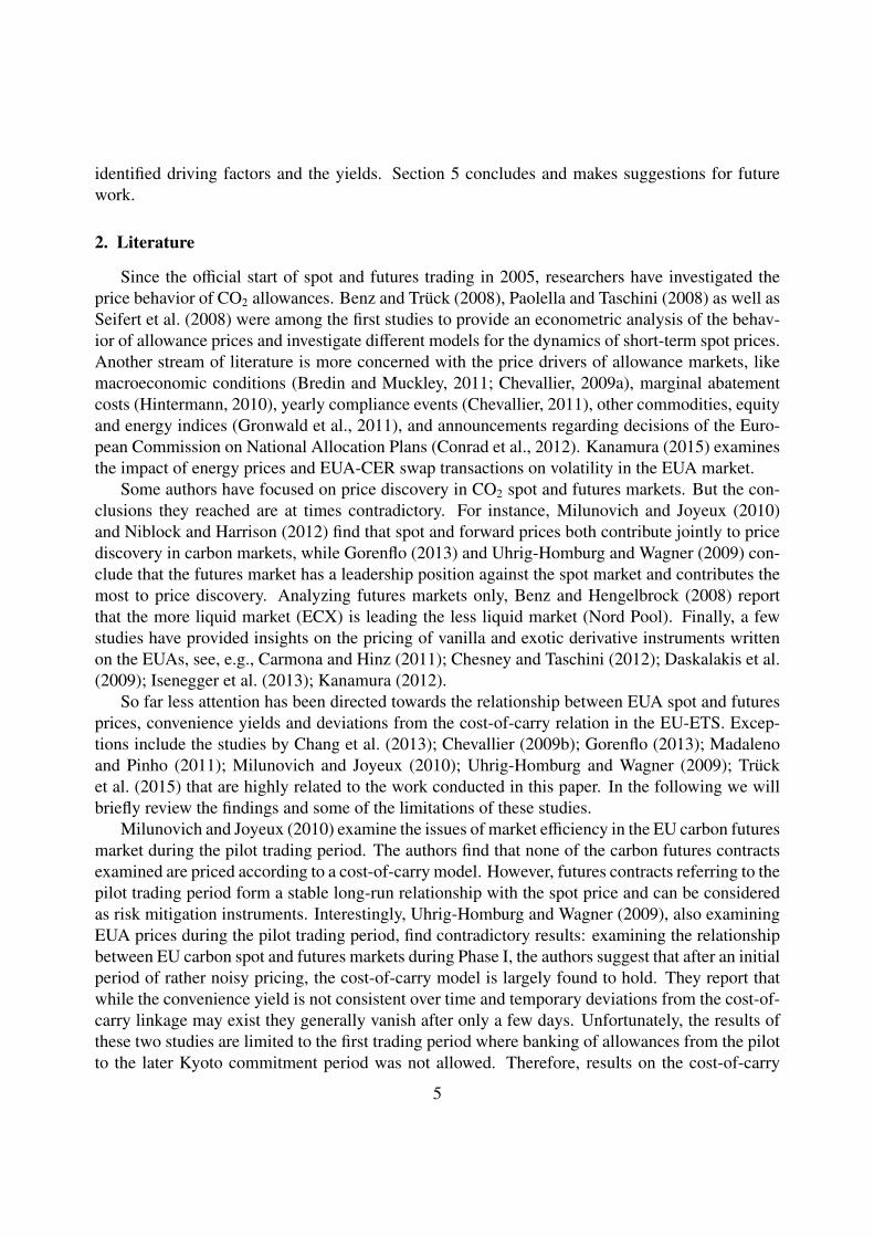
April 8, 2008 to December 31, 2012. Figure 1 provides the spot price series as well as December2010, 2012 and 2014 futures price for the period considered.4 We observe that the Phase II EUAspot price (bold solid line) on April 8, 2008 was EUR 23.53 and initially increased to its maximumlevel of EUR 29.38 on July 1, 2008. What followed was a relatively rapid decline in prices downto EUR 8.00 on February 12, 2009 which can mainly be attributed to the impacts of the financialcrisis and lower expectations about economic output in the Eurozone due to the crisis. Spot pricesincreased again up to a level of EUR 15.45 in May 2009 and remained in the range EUR 13–16up to June 2011. Since then, due to the European Sovereign Debt crisis, expectations about lowereconomic output and emissions below the actual annual allocation of allowances, prices droppedto a level of approximately EUR 6.50 in December 2012. We also observe that spot and futuresprices show a similar price behavior during the considered time period.

3These exchanges were chosen, since they provide a high level of liquidity, see, e.g. Mizrach and Otsubo (2014).4Note that the 2010 futures contract expired on December 20, 2010, the 2012 futures contract on December 17,

2012, while the first price observation for the 2014 futures contract was available on December 21, 2010.

10

0 200 400 600 800 1000 12005

10

15

20

25

30

35

Days (2008/04/08 − 2012/12/31)

Spo

t / F

utur

es P

rice

Figure 1: Spot price (solid black), December 2010 (dashed), December 2012 (dotted) and December 2014 (solid grey)futures price for the first Kyoto commitment period April 8, 2008 to December 31, 2012. The December 2010 futurescontract expired on December 20, 2010, the December 2012 futures contract on December 17, 2012, while the firstprice observation for the 2014 futures contract was available on December 21, 2010.

The co-movement of spot and futures contracts during the first Kyoto commitment period isalso confirmed by looking at the correlation coefficients between returns from spot and consideredfutures contracts in Table 1. We find that correlations between spot and futures returns are all wellabove 0.95 and close to one. This is also true for futures contracts referring to Phase III, althoughcorrelations between Phase II spot and futures returns and the 2015 futures contracts are slightlylower than for most of the other contracts.

In a next step, using equation (3) we calculate convenience yields for the 2009-2015 futurescontracts. Summary statistics for the estimated convenience yields are reported in Table 2. Wefind negative average convenience yields for all futures contracts, while the absolute value of theyields increases for contracts with longer maturities. While for Phase II futures contracts themean of observed convenience yields has a range between roughly -1% for the 2009 contract and-2.14% for the 2012 contract, for Phase III average convenience yields are between -3.68% forthe 2013 contract and -5.03% for the 2015 contract. Clearly, for Phase III the market indicatessubstantial negative convenience yields, in magnitude well above the level of the risk-free rate,such that (rT−t − cT−t) > 0 and, therefore, Phase III futures prices are typically significantly higherthan the spot. This behavior is also illustrated in Figure 1, where the relatively large deviation of2014 futures prices from the spot price is displayed. Interestingly, we also find that the standarddeviation of convenience yields decreases for longer maturity of the futures contract. It is thehighest for the convenience yield of the nearest term 2009 futures (σ = 0.0156) and by far thelowest for the 2015 futures contract (σ = 0.0057). These results are in line with the proposedtime-to-maturity or Samuelson effect for commodity markets (Samuelson, 1965) that suggests atypically declining term structure in the volatility of futures prices as maturity increases. Thebehavior is generally explained by the fact that only few of the parameters affecting the opinionof investors about distant futures prices will change today. Hence, only minor effects are expected

11

Delivery Spot 2009 2010 2011 2012 2013 2014 2015Spot 1.0000 0.9915 0.9809 0.9708 0.9689 0.9897 0.9888 0.95802009 1.0000 0.9895 0.9797 0.9794 - - -2010 1.0000 0.9870 0.9779 0.9784 - -2011 1.0000 0.9774 0.9863 0.9819 -2012 1.0000 0.9955 0.9944 0.96262013 1.0000 0.9970 0.96672014 1.0000 0.96802015 1.0000

Table 1: Correlations between returns from spot and 2009-2015 futures contracts for Kyoto commitment period marketquotes from April 8, 2008 to December 31, 2012. Note that correlation coefficients between returns from the 2009and 2013, 2014 and 2015 futures contracts could not be calculated because the 2009 contract expired before quotes forthese contracts were available. The same is true for the correlation coefficient between 2010 and 2014, 2015 contractsand for 2011 and 2015 futures contracts.

Contract 2009 2010 2011 2012 2013 2014 2015Mean -0.0099 -0.0107 -0.0144 -0.0214 -0.0368 -0.0435 -0.0503Median -0.0116 -0.0125 -0.0152 -0.0205 -0.0346 -0.0447 -0.0508Std 0.0156 0.0121 0.0114 0.0120 0.0112 0.0112 0.0057Min -0.0417 -0.0506 -0.0636 -0.0626 -0.0737 -0.0661 -0.0633Max 0.0307 0.0285 0.0264 0.0230 -0.0204 -0.0200 -0.0303Obs 411 670 924 1131 773 515 261

Table 2: Descriptive statistics for convenience yields for 2009 - 2015 futures contracts. The 2009 futures contractexpired on December 14, 2009, the 2010 futures contract expired on December 20, 2010, the 2011 contract onDecember 19, 2011 and the 2012 contract on December 17, 2012. Phase III futures contract prices were availablefrom December 16, 2009 (2013 futures), December 21, 2010 (2014 futures) and December 20, 2011 (2015 futures).

for futures with long maturities, even if there are more significant changes to the spot price ornear-term futures contracts.

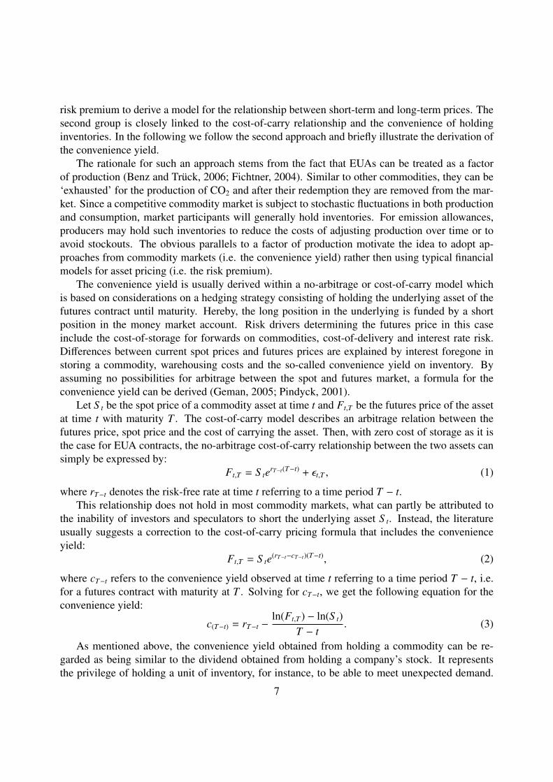
Figure 2 provides a plot of the observed convenience yields for the December 2009, 2011 and2012 futures contracts based on the cost-of-carry relationship described in Section 3. We observethat the market started in backwardation, with positive convenience yields, indicating that the spotprice was above the discounted price of Kyoto commitment period futures contracts. In the courseof time, the market situation changed from backwardation to contango for the first time in July2008. Prices were approximately in line with the cost-of-carry relationship until end of October2008, but afterwards convenience yields become negative. For most of the time after January2009, convenience yields for the 2010, 2011 and 2012 futures contracts are significantly smallerthan zero. Thus, we find that none of the spot or futures contracts were priced according to the cost-of-carry relationship. The effect is more pronounced for futures contracts with longer maturities,i.e. the December 2011 and 2012 futures contracts. We also observe that as the contracts get closerto the expiry date, the convenience yield becomes more volatile.

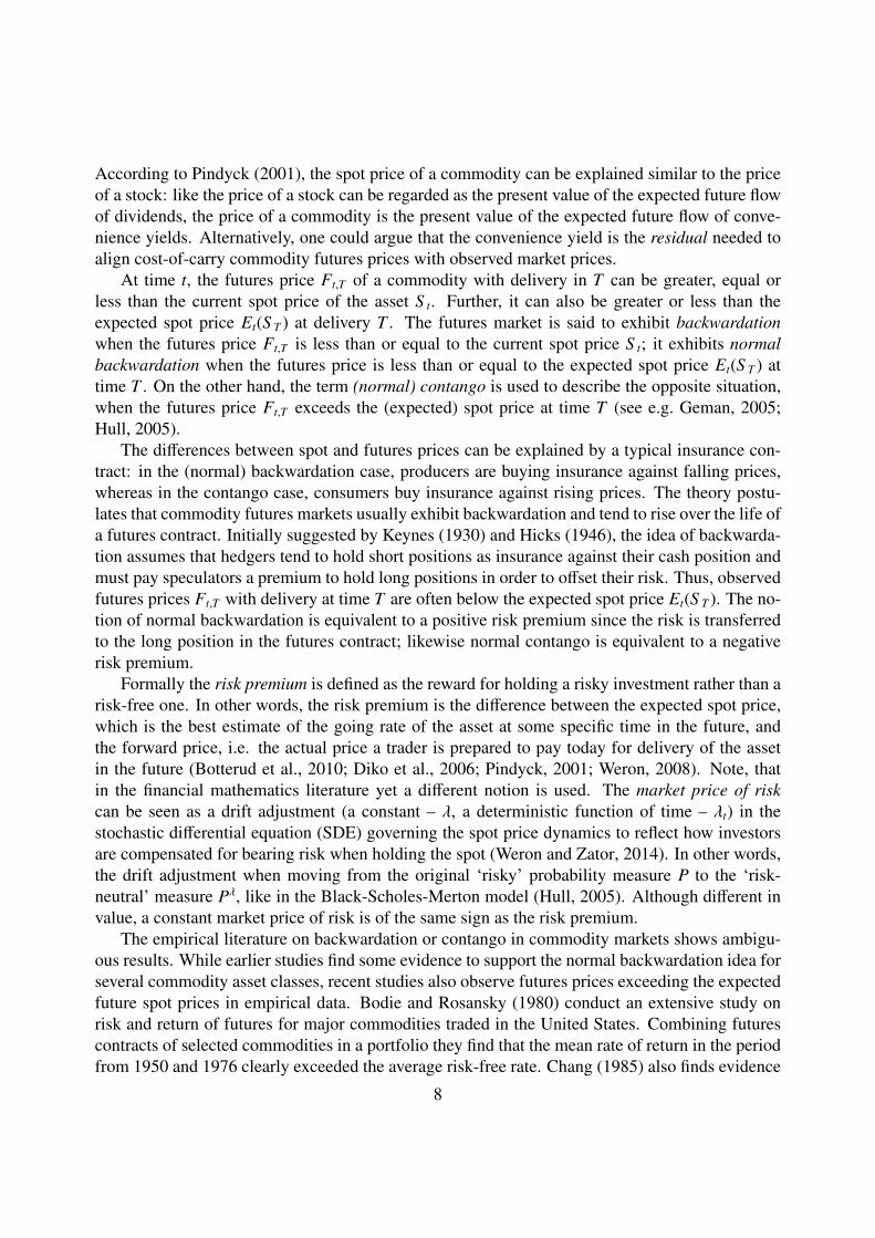
Figure 3 displays the results for the relationship between Phase II spot and Phase III futures

12

0 200 400 600 800 1000 12005

10

15

20

25

30

Spo

t Pric

e

0 200 400 600 800 1000 1200

−0.06

−0.04

−0.02

0

0.02

0.04

Spot Price

Con

veni

ence

Yie

ld

Figure 2: Upper panel: Spot prices (EUR/ton) from April 8, 2008 to December 31, 2012. Lower panel: Convenienceyields (EUR/ton) for 2009 (solid black), 2011 (dashed black) and 2012 (solid grey) EUA futures contracts. The 2009futures contract expired on December 14, 2009, the 2011 contract on December 19, 2011 and the 2012 contract onDecember 17, 2012.

0 200 400 600 800 1000 12005

10

15

20

25

30

Spo

t Pric

e

0 200 400 600 800 1000 1200−0.08

−0.06

−0.04

−0.02

0

Con

veni

ence

Yie

ld

Figure 3: Upper panel: Spot prices (EUR/ton) from December 16, 2009 to December 31, 2012. Lower panel:Convenience yields (EUR/ton) for December 2013 (solid black), December 2014 (dotted black) and December 2015(solid grey) EUA futures contracts. Phase III futures contract prices were available from December 16, 2009 (2013futures), December 21, 2010 (2014 futures) and December 20, 2011 (2015 futures).

13

contracts. Note that inter-period banking between the phases is allowed such that the EU-ETSenables market participants to use Phase II permits also during Phase III. On the other hand,borrowing of permits from Phase III and using the allowances in Phase II is not allowed. Pricesfor the considered Phase III futures contracts were only available from December 16, 2009 (2013futures), December 21, 2010 (2014 futures) and December 20, 2011 (2015 futures). Therefore, thelower panel of Figure 3 only provides a plot of the convenience yields for this time period. We findhighly negative convenience yields for all Phase III futures contracts, usually in the range between-2% and -7%. In the year 2012, observed convenience yields have been reduced in magnitude,however, they remain below -2% for all contracts during the entire time period.

Note that our findings with respect to a clear deviation from the cost-of-carry relationship forPhase II are in line with earlier work examining EUA spot and futures contracts during the Ky-oto commitment period (Chang et al., 2013; Gorenflo, 2013; Madaleno and Pinho, 2011; Trucket al., 2015). However, the consistently negative sign of observed convenience yields from March2009 onwards, at least partially contradicts results reported in some of these studies. Madalenoand Pinho (2011) and Chang et al. (2013) report positive convenience yields during late 2009 and2010 for some of the futures contracts (usually contracts with maturity during Phase II, i.e. expiryin December 2010, 2011 or 2012). The key reason for the deviation in our results, may be differentassumptions about the risk-free rate. While Madaleno and Pinho (2011) assume a constant interestrate for the estimation period of 4%, Chang et al. (2013) choose a constant free-risk rate equal tothe average coupon rate of 3.06%, i.e. the rate for three-year government bonds issued in 2010 inthe European Union. Also Gorenflo (2013) state that the interest rate is assumed to be constantover time in his analysis. Note that in our study we do not assume a constant risk-free rate, butdecided to use actual daily European Central Bank (ECB) quotes for AAA-rated euro area centralgovernment bonds for different maturities. Further, to match the yields for different time horizonsuntil maturity of the considered futures contracts we use linear interpolation between quoted inter-est rates. As mentioned earlier, risk-free rates in the Eurozone have dropped significantly from alevel of around 4% in September 2008 to a level below 1% since late September 2009. Therefore,it is no surprise that in our analysis we obtain different results in comparison to previous studies,where significantly higher interest rates have been applied.

Overall, the negative convenience yields for Kyoto period futures contracts from 2009 onwardsindicate that market participants saw no privilege in holding the allowance now with respect to fu-ture periods. We find that long positions in futures contracts are priced at a much higher levelthan suggested by the cost-of-carry relationship. Generally, a contango market as it is observedduring Phase II would suggest currently available supply but potential medium-to-long-term short-ages of a commodity. Under such a scenario, consumers might be interested in buying insuranceagainst rising prices in the futures market. Therefore, a greater interest in long futures positionswill drive prices of these contracts up. Observed negative convenience yields may be interpretedas consumers’ willingness to pay an additional risk premium for a hedge against rising prices orfuture shortage of EUAs. Clearly, it can also be interpreted as a hedge against potential changesin regulation that may reduce the availability of permits in forthcoming years.

As banking and borrowing within the years of the Kyoto commitment period (i.e. 2008-2012)is allowed, one could also argue that the deviation from the cost-of-carry relationship may be dueto different market expectations about interest rates in forthcoming years. Although firms tend to

14

Apr 2008 Jan 2009 Nov 2009 Aug 2010 May 2011 March 2012 Dec 2012−0.5

0

0.5

1

1.5

2

2.5

3

3.5

4

4.5

Sho

rt−

Ter

m In

tere

st R

ate

Figure 4: Daily short term (3-month) European Central Bank (ECB) quotes for AAA-rated Euro area central govern-ment bonds from April 8, 2008 to December 31, 2012.

use banking provisions in a rational way, as reported by Ellerman and Montero (2007) for the USAcid Rain Program, the increasing surplus levels and banking of EUAs might suggest expectedrelatively low scarcity of the allowances at time t versus some time in the future T , i.e. the maturityof the futures contracts. This encourages us to analyze the behavior of observed convenience yieldswith regards to possible drivers of the yields in more detail.

4.3. Driving factors of the Convenience YieldIn the following, we try to explain the observed deviations from the cost-of-carry relationship

by a number of exogenous variables. In particular we attribute the existence of negative con-venience yields of relatively high absolute magnitude to the following factors: (i) interest ratelevels in the Eurozone, (ii) the increasing level of surplus allowances and banking during PhaseII, and (iii) market participants’ willingness to pay an additional risk premium for a hedge againstuncertainty about EUA price behavior and possibly rising prices in future periods.

4.3.1. Interest RatesThe first reason for observing negative convenience yields may be the extremely low risk-

free rates in the Eurozone from 2009 onwards. The drop of the risk-free rate from roughly 4%in early 2008 to a rate near 0.5% from January 2009 onwards was initially due to the globalfinancial crisis, while yields for AAA-rated government bonds have remained at such low levelsever since. Interest rates can be expected to impact on the relationship between commodity spotand futures prices and have been suggested as a pricing factor for commodity derivatives, see e.g.Casassus and Collin-Dufresne (2005); Schwartz (1997); Schwartz and Smith (2000). Note thatin the three-factor model developed by Casassus and Collin-Dufresne (2005), the convenienceyield can be dependent on the risk-free rate itself. As indicated by equations (3) and (4), therisk-free rate is also a key input in the cost-of-carry model and, therefore, will have an impact ondeviations from this relationship and the calculation of the convenience yield. We also observethat convenience yields become more significant once risk-free rates in the Eurozone drop to thelow levels observed since 2009. During periods of very low interest rates it may be more likely to

15

observe negative convenience yields for risky assets. This could be a result of market expectationsabout rising interest rates in forthcoming periods. We use daily short term (3-month) EuropeanCentral Bank (ECB) quotes for AAA-rated Euro area central government bonds as a proxy forthe risk-free spot rate in our analysis. Figure 4 provides a plot of the interest rate applied in theanalysis. We formulate the following hypothesis about the relationship between the risk-free rateand convenience yields in the EU-ETS:

Hypothesis 1: Lower interest rates will decrease the convenience yield, such that we expect apositive relationship between interest rates and observed convenience yields.

Based on Hypothesis 1, we would therefore expect a positive coefficient, when regressing conve-nience yields on short-term interest rates.

4.3.2. BankingThe second explanation refers to the possibility of banking EUAs and the surplus of allowances

available during Phase II. Generally, the theory of storage suggests a negative relationship betweenthe convenience yield and inventory, see e.g. Pindyck (2001). The owner of a commodity, whois free to consume it until maturity, is prepared for unexpected shortages in supply or increases indemand. The convenience yield then represents this additional benefit of holding a unit of inven-tory, for instance, to be able to meet unexpected demand. The value of this benefit should then benegatively related to the level of inventory. One could argue that it is particularly high if invento-ries of a commodity are low and consumers are forced to secure a short-term supply. On the otherhand, high levels of inventory will reduce the benefits and, therefore, also the convenience yield.Considering the continuously increasing level of surplus allowances during the first Kyoto com-mitment period (Ellerman et al., 2014; Zaklan et al., 2014) and the extensive use of external creditscoming from two of the Kyoto Protocol mechanisms, the clean development mechanism (CDM)and joint implementation (JI), one could argue that throughout Phase II an increasingly higherlevel of inventory was accumulated.5 Therefore, the change in the market from backwardation tocontango and significantly negative convenience yields for futures contracts could be a result of anincreasing level of surplus allowances and banking. We formulate the following hypothesis aboutthe relationship between surplus allowances and observed convenience yields:

Hypothesis 2: An increase in the number of surplus allowances will decrease the benefit of holdingspot contracts in comparison to a position in a futures contract. Thus, we expect a negativerelationship between the EUA bank and observed convenience yields.

Data on allowance banking behavior are available in the European Union Transaction Log (EUTL)and comprise installation-level information on free allocations, verified emissions and surrendersof both EUAs and Kyoto offsets against emissions (Zaklan et al., 2014). Note that in order tocompute the correct size of the bank at a sub-system level, we would also require information onsales and purchases of EUAs. Unfortunately, for this level of detail, data are not available until

5See also http://europeanclimatepolicy.eu/.

16

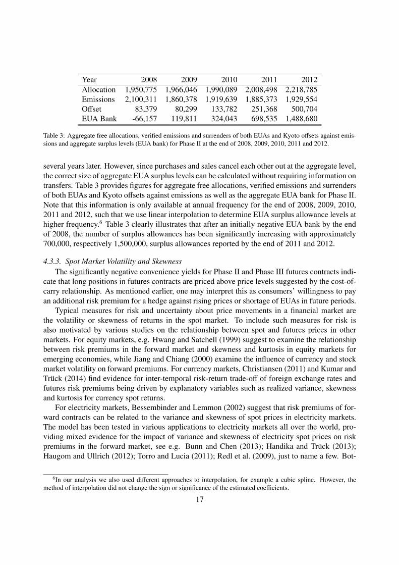
Year 2008 2009 2010 2011 2012Allocation 1,950,775 1,966,046 1,990,089 2,008,498 2,218,785Emissions 2,100,311 1,860,378 1,919,639 1,885,373 1,929,554Offset 83,379 80,299 133,782 251,368 500,704EUA Bank -66,157 119,811 324,043 698,535 1,488,680

Table 3: Aggregate free allocations, verified emissions and surrenders of both EUAs and Kyoto offsets against emis-sions and aggregate surplus levels (EUA bank) for Phase II at the end of 2008, 2009, 2010, 2011 and 2012.

several years later. However, since purchases and sales cancel each other out at the aggregate level,the correct size of aggregate EUA surplus levels can be calculated without requiring information ontransfers. Table 3 provides figures for aggregate free allocations, verified emissions and surrendersof both EUAs and Kyoto offsets against emissions as well as the aggregate EUA bank for Phase II.Note that this information is only available at annual frequency for the end of 2008, 2009, 2010,2011 and 2012, such that we use linear interpolation to determine EUA surplus allowance levels athigher frequency.6 Table 3 clearly illustrates that after an initially negative EUA bank by the endof 2008, the number of surplus allowances has been significantly increasing with approximately700,000, respectively 1,500,000, surplus allowances reported by the end of 2011 and 2012.

4.3.3. Spot Market Volatility and SkewnessThe significantly negative convenience yields for Phase II and Phase III futures contracts indi-

cate that long positions in futures contracts are priced above price levels suggested by the cost-of-carry relationship. As mentioned earlier, one may interpret this as consumers’ willingness to payan additional risk premium for a hedge against rising prices or shortage of EUAs in future periods.

Typical measures for risk and uncertainty about price movements in a financial market arethe volatility or skewness of returns in the spot market. To include such measures for risk isalso motivated by various studies on the relationship between spot and futures prices in othermarkets. For equity markets, e.g. Hwang and Satchell (1999) suggest to examine the relationshipbetween risk premiums in the forward market and skewness and kurtosis in equity markets foremerging economies, while Jiang and Chiang (2000) examine the influence of currency and stockmarket volatility on forward premiums. For currency markets, Christiansen (2011) and Kumar andTruck (2014) find evidence for inter-temporal risk-return trade-off of foreign exchange rates andfutures risk premiums being driven by explanatory variables such as realized variance, skewnessand kurtosis for currency spot returns.

For electricity markets, Bessembinder and Lemmon (2002) suggest that risk premiums of for-ward contracts can be related to the variance and skewness of spot prices in electricity markets.The model has been tested in various applications to electricity markets all over the world, pro-viding mixed evidence for the impact of variance and skewness of electricity spot prices on riskpremiums in the forward market, see e.g. Bunn and Chen (2013); Handika and Truck (2013);Haugom and Ullrich (2012); Torro and Lucia (2011); Redl et al. (2009), just to name a few. Bot-

6In our analysis we also used different approaches to interpolation, for example a cubic spline. However, themethod of interpolation did not change the sign or significance of the estimated coefficients.

17

terud et al. (2010) and Weron and Zator (2014) investigate convenience yields in the Nord Poolelectricity market and find a significant relationship between the yields and spot price variance andskewness. For the relationship between EUA spot and futures contracts, Chevallier (2009b) andMadaleno and Pinho (2011) also regress observed convenience yields on measures of volatility inthe spot market. However, their analysis is limited to either data from the pilot trading period onlyor observations up to 2009.

Motivated by this line of research, we examine the impact of volatility and skewness in theEUA spot market on the observed convenience yields during the first Kyoto commitment period.We apply an exponentially weighted moving average (EWMA) to model the volatility in the EUAspot market, where the variance estimate σ2

t for returns in the EUA spot market for day t is basedon the following relationship:

VARt ≡ σ2t = λσ2

t−1 + (1 − λ)r2t−1, (4)

with σ2t−1 being the previous day’s estimate for the variance and r2

t−1 the square of the most recentEUA return observation.7 The estimated variance at each point in time is then used as an explana-tory variable for the observed convenience yields. We formulate the following hypothesis aboutthe relationship between variance in the EUA spot market and the convenience yields:

Hypothesis 3: Increased variance in the spot market, will increase the demand for hedging and,therefore, increase futures prices. Thus, we expect a negative relationship between spot marketvolatility and observed convenience yields.

4.4. The Convenience Yield ModelsIn the following we will describe the results for the applied models for the dynamics of the

observed convenience yields. Recall that due to expiry of the futures contracts and a later start oftrading for some of the Phase III contracts, we do not observe prices for all contracts throughoutthe entire sample period (April 8, 2008 - December 31, 2012). For example, the 2009, 2010 and2011 futures contracts expired at least a year before the end of the sample period, while pricesfor the 2014 futures contract were only available from December 21, 2010.8 Therefore, we havean unbalanced data set, where convenience yields for contracts i = 1, ..., 7 are observed differentnumber of times Ti. Hereby i = 1 refers to the 2009 futures contract, i = 2 to the 2010 futurescontract and so on.

We first investigate the dynamics of the convenience yields using a pooled OLS estimator(Model I)

CYi,t = β0 + β1INTt + β2BANKt + β3VARt + εi,t, (5)

7We use λ = 0.94 for the smoothing parameter, following the approach suggested in RiskMetricsT M . Note thatwe also applied alternative values for the smoothing parameter λ as well as a GARCH(1,1) model for the conditionalvolatility of EUA returns. However, the different approaches did not change the sign and significance of the estimatedcoefficients in the applied regression models and gave very similar results.

8See Table 2 for details on trading dates and the number of observations on convenience yields for each of the2009-2015 futures contracts.

18

where INTt denotes the short term (3-month) interest rate in the Eurozone area at time t, BANKt

is an estimate of the number of EUA surplus allowances at time t, VARt is the estimated volatilityin the EUA spot market at time t based on the applied EWMA model, see equation (4), and εi,t isthe noise term, assumed to be independent and identically distributed with mean zero and finitevariance.

As mentioned above, the literature (Bessembinder and Lemmon, 2002; Christiansen, 2011;Kumar and Truck, 2014) suggests that also returns in the spot market as well as higher momentsof spot price returns may have an impact on risk premiums in the futures markets. These riskpremiums would then also be reflected in observed convenience yields for CO2 futures contracts.Therefore, we also apply an extended model, where we include the estimated skewness SKEWt

and the most recent return rt in the EUA spot market at time t. To model skewness we apply arolling estimator based on the last k daily returns:

SKEWt =1

k − 1

k∑i=1

(ri − r)3

σt, (6)

where σt denotes the standard deviation and r the average of EUA spot returns during the last ktrading days. We choose k = 20 what roughly corresponds to the skewness of returns in the EUAspot market during the last month and formulate the following extended model (Model II):

CYi,t = β0 + β1INTt + β2BANKt + β3VARt + β4rt + β5SKEWt + εi,t. (7)

Note, however, that given the substantial differences between the magnitude of observed con-venience yields for the 2009-2015 contracts (see Table 2), the assumption of a common constantterm for all contracts in Model I and Model II may not be appropriate. Recall that for Phase IIIfutures contracts, we found the convenience yields far more pronounced (in absolute terms) incomparison to Phase II contracts. To further investigate this issue, we also run the pooled regres-sion with additional dummy variables to distinguish between individual future contracts.

First, we consider a model that distinguishes between futures contracts with expiry date inPhase II and Phase III, by introducing a dummy variable dphaseIII with dphaseIII = 1 for observationsfor contracts i = 5, 6, 7.

Thus, Model III becomes

CYi,t = β0 + β1INTt + β2BANKt + β3VARt + γdphaseIII + εi,t, (8)

while in Model IV we simply include the Phase III dummy variable into the equation for Model II.We also consider a model with separate dummy variables for the individual contracts to further

address heterogeneity in the convenience yields for the traded EUA futures. Thus, we define di = 1for observations of futures contracts i = 2, 3, ..., 7 and di = 0 otherwise. To avoid the ’dummyvariable trap’, no dummy is used for the 2009 contract (i = 1). Thus, the model including dummyvariables for the individual contracts (Model V) takes the following form:

CYi,t = β0 + β1INTt + β2BANKt + β3VARt +

7∑i=2

γidi + εi,t. (9)

19

Then running the pooled OLS regression, γ2 denotes the coefficient on d2, γ3 is the coefficienton d3, and so on. Note that this model is typically referred to as the dummy variable regression andthe estimators for β1, β2, β3 will be identical to the fixed effects estimators, see, e.g. Wooldridge(2010). It is straightforward to also include the contract dummy variables into the extended ModelII, what yields Model VI.

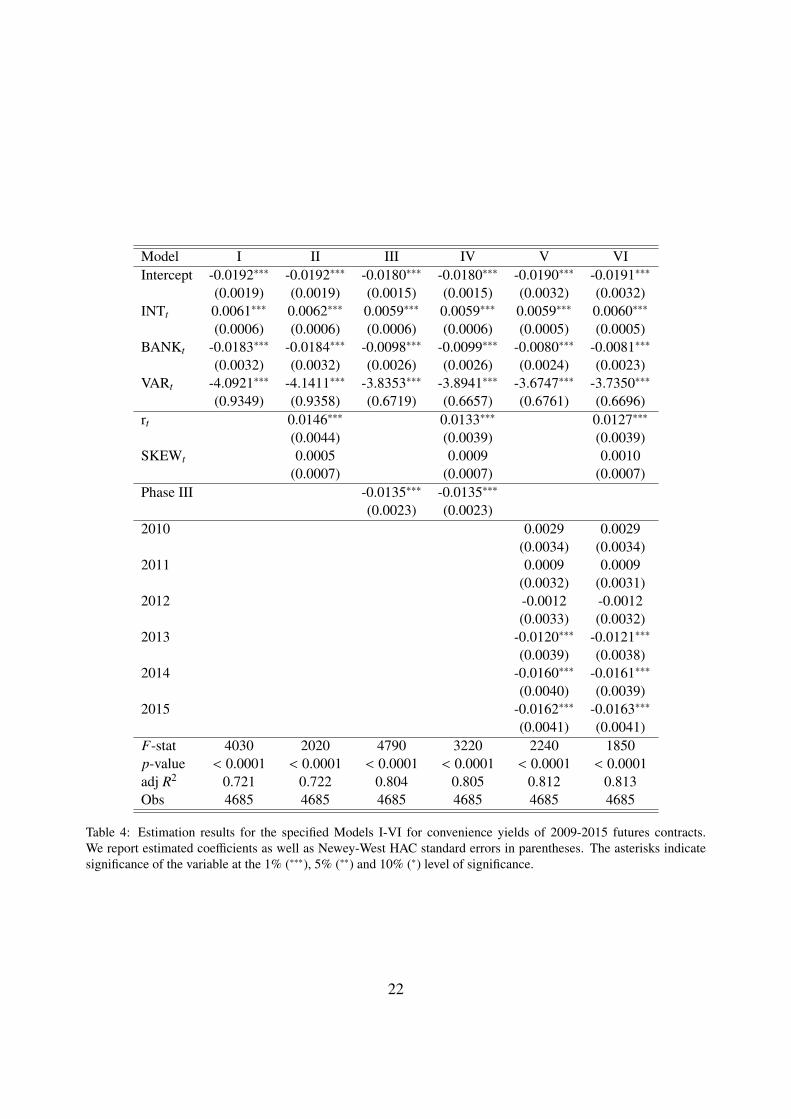
Results for the considered six models are provided in Table 4. We report estimated coeffi-cients as well as Newey-West HAC adjusted standard errors to account for autocorrelation andheteroskedasticity in the explanatory and dependent variables.

Examining the results for the most basic Model I, see equation (5), we observe that all estimatedcoefficients are significant at the 1% level and show the expected signs according to Hypothesis1-3. The relationship between interest rates and convenience yields is positive, suggesting that thedrop in risk-free rates during the financial crisis period and the subsequent low interest rate envi-ronment has also had a significant impact on convenience yields in the EU-ETS futures market.We also find evidence for the negative relationship between the convenience yield and inventory asit has been suggested in the theory of storage, confirming Hypothesis 2. Thus, the rising numberof surplus allowances throughout the sample period has led to a further decrease in convenienceyields for EUA futures. Furthermore, we find a significant negative relationship between the vari-ance of spot prices and convenience yields. Therefore, increased price volatility in the EUA spotmarket will decrease convenience yields, indicating that market participants are willing to pay anadditional risk premium in the futures market for a hedge against increased uncertainty about EUAprices. We also find that the simple specification of Model I provides a relatively high explanatorypower of R2 = 0.721, suggesting more than 70% of the variation in convenience yields for thefutures contracts can be explained by the proposed variables.

Comparing these results to Model II, see equation (7), we observe that including additionalvariables capturing the most recent return in the EUA spot market as well as a measure for skew-ness in the spot market does not increase the explanatory power of the model by a huge margin.The estimated coefficient for skewness is insignificant, indicating that market participants are moreconcerned with volatility in the spot market than with higher moments of the return distribution.However, the coefficient for returns in the spot market rt is positive, suggesting that an increase inspot prices will increase convenience yields. Given that convenience yields throughout the sam-ple period were typically negative, this suggests that overall the deviation from the cost-of carryrelationship is reduced with increasing spot prices.

Let us now consider the results for Models III-VI, including additional dummy variables forspecific futures contracts. For Model III and Model IV, we find a highly significant coefficientγ = −0.0135 for the Phase III dummy variable. As expected, the model confirms that convenienceyields for Phase III futures contracts are significantly more negative (of greater magnitude in abso-lute terms), what is also indicated in Table 2. Including dphaseIII into the model also increases theexplanatory power from R2 = 0.721 to R2 = 0.804 (Model I in comparison to Model III), and fromR2 = 0.722 to R2 = 0.805 (Model II in comparison to Model IV), respectively. However, theseresults also point towards heterogeneity across individual contracts, questioning the consistenceof the OLS estimates in the most simple model specifications (5) and (7). We find that while thesigns and significance of the estimated coefficients remain unaffected, the estimates of the coeffi-cients are changed. While the effects are rather small for β1 (coefficient for the interest rate), the

20

coefficients β2 (banking) and β3 (variance in the spot market) show more considerable changes,for example from β2 = −0.0183 (Model I)to β2 = −0.0098 (Model III) and from β3 = −4.0921(Model I) to β3 = −3.8353 (Model III), respectively. At the same time the standard error of theestimates for these variables is reduced, since some of the heterogeneity is picked up by the intro-duced Phase III dummy variable. However, all signs as well as the significance of the coefficientsremain unchanged, emphasizing the importance of the variables as driving factors of the observedconvenience yields.

Further investigating the issue of heterogeneity, we consider results for Model V and Model VIthat include dummy variables for the individual contracts in the pooled OLS estimation. Note thatas pointed out before, this specification can be considered as a convenient way to carry out fixedeffect analysis (Wooldridge, 2010), what seems to be more appropriate given the heterogeneityacross individual contracts. We find that none of the dummy variables for Phase II futures contractsis significant, while all dummies for Phase III contracts are negative and significant at the 1%level. Estimates for γ5 − γ7, i.e., 2013, 2014 and 2015 futures contracts for Model V range fromγ5 = −0.0120 to γ7 = −0.0162, with similar results for the extended Model VI. Using individualdummies for the contracts further increases the explanatory power of the model to R2 = 0.812(Model V) and R2 = 0.813 (Model VI). Again, estimated coefficients for the interest rate β1 onlyexhibit minor changes, while the coefficients β2 (banking) and β3 (variance in the spot market)again exhibit more considerable changes. For example, Model V yields β2 = −0.0080 and β3 =

−3.6747 in comparison, while the standard error of the estimates is further reduced as a resultof introducing the contract specific dummy variables. So our results point towards inconsistentestimates of a standard pooled OLS model, and suggest the use of a fixed effect or dummy variableestimator.

At the same time, the results for Model V and Model VI illustrate that a large variation in thedynamics of the observed convenience yields is actually explained by the suggested explanatoryvariables. All variables remain significant and show the expected sign, in line with the formulatedHypothesis 1-3.

Overall, our results provide strong evidence for the impact of the suggested variables as keydrivers of observed convenience yields dynamics during Phase II. With regards to Hypothesis 1,we find that lower risk-free interest rates decrease observed convenience yields in the EU-ETS.For all model specifications I-VI, the estimated coefficients are positive and significant at the 1%level, suggesting that the drop in short-term interest rates has contributed to the change from initialbackwardation to contango for the market and the decline in convenience yields.

We also find strong evidence for the impact of the increased number of surplus allowanceson the convenience yields as stated in Hypothesis 2. Our models yield a negative coefficientfor the banking variable, suggesting that the rising number of surplus allowances has led to afurther decrease in observed convenience yields during Phase II. While the absolute magnitudeof the coefficients becomes smaller, when additional dummy variables for the trading periods orindividual contracts are included into the model, for all model specifications the coefficients remainhighly significant at the 1% level. Thus, our results confirm the negative relationship between theconvenience yield and inventories as it has been suggested for other commodity markets (Pindyck,2001).

Considering the relationship between volatility in the EUA spot market and the convenience

21

Model I II III IV V VIIntercept -0.0192∗∗∗ -0.0192∗∗∗ -0.0180∗∗∗ -0.0180∗∗∗ -0.0190∗∗∗ -0.0191∗∗∗

(0.0019) (0.0019) (0.0015) (0.0015) (0.0032) (0.0032)INTt 0.0061∗∗∗ 0.0062∗∗∗ 0.0059∗∗∗ 0.0059∗∗∗ 0.0059∗∗∗ 0.0060∗∗∗

(0.0006) (0.0006) (0.0006) (0.0006) (0.0005) (0.0005)BANKt -0.0183∗∗∗ -0.0184∗∗∗ -0.0098∗∗∗ -0.0099∗∗∗ -0.0080∗∗∗ -0.0081∗∗∗

(0.0032) (0.0032) (0.0026) (0.0026) (0.0024) (0.0023)VARt -4.0921∗∗∗ -4.1411∗∗∗ -3.8353∗∗∗ -3.8941∗∗∗ -3.6747∗∗∗ -3.7350∗∗∗

(0.9349) (0.9358) (0.6719) (0.6657) (0.6761) (0.6696)rt 0.0146∗∗∗ 0.0133∗∗∗ 0.0127∗∗∗

(0.0044) (0.0039) (0.0039)SKEWt 0.0005 0.0009 0.0010

(0.0007) (0.0007) (0.0007)Phase III -0.0135∗∗∗ -0.0135∗∗∗

(0.0023) (0.0023)2010 0.0029 0.0029

(0.0034) (0.0034)2011 0.0009 0.0009

(0.0032) (0.0031)2012 -0.0012 -0.0012

(0.0033) (0.0032)2013 -0.0120∗∗∗ -0.0121∗∗∗

(0.0039) (0.0038)2014 -0.0160∗∗∗ -0.0161∗∗∗

(0.0040) (0.0039)2015 -0.0162∗∗∗ -0.0163∗∗∗

(0.0041) (0.0041)F-stat 4030 2020 4790 3220 2240 1850p-value < 0.0001 < 0.0001 < 0.0001 < 0.0001 < 0.0001 < 0.0001adj R2 0.721 0.722 0.804 0.805 0.812 0.813Obs 4685 4685 4685 4685 4685 4685

Table 4: Estimation results for the specified Models I-VI for convenience yields of 2009-2015 futures contracts.We report estimated coefficients as well as Newey-West HAC standard errors in parentheses. The asterisks indicatesignificance of the variable at the 1% (∗∗∗), 5% (∗∗) and 10% (∗) level of significance.

22

yield, we find unambiguous support for Hypothesis 3. There is a significant negative relationshipbetween spot market volatility and observed convenience yields such that increased variance in thespot market further decreases the convenience yield. These findings suggest that higher volatilityand rising uncertainty about EUA price behavior significantly increases the demand for hedgingand leads to an increase in observed futures prices. As a result, EUA futures prices exhibit strongcontango, in particular during periods of higher volatility in the spot market. Similar results havealso been obtained for electricity markets, where, for example, Botterud et al. (2010), Handikaand Truck (2013), Redl et al. (2009) and Weron and Zator (2014) find a significant relationshipbetween risk premiums or convenience yields and spot price variance.

With regards to including additional explanatory variables into the model, we find that returnsand skewness in the EUA spot market do not provide a significant increase in the explanatorypower of the models. The estimated coefficient for skewness is not significant in any of the models.However, the estimated coefficient for spot returns is significant and positive, suggesting that aprice increase in the spot market will typically reduce the magnitude of the (negative) convenienceyield. Thus, rising spot prices have a tendency to reduce the deviation from the cost-of-carryrelationship and, therefore, consumers’ willingness to pay an additional risk premium in the futuresmarket.

5. Conclusions and Policy Implications

We provide an empirical study on convenience yields in CO2 allowance futures prices duringthe first Kyoto commitment period from 2008 to 2012. In particular, we examine deviations fromthe cost-of-carry relationship for Phase II and Phase III futures contracts and the driving factorsfor the dynamics of observed convenience yields for emission allowances. While the connectionbetween spot and futures markets has been thoroughly investigated for other commodities such asoil, electricity, gas or agricultural products, so far only a small number of studies have analyzedthe convenience yield and risk premiums in the EU-ETS.

Our findings suggest that during the considered sample period,i.e. the first Kyoto commitmentperiod, the EUA market has changed from an initial short period of backwardation to contangowith significant negative convenience yields. Observed average yields range from -1% to -2% forcontracts with delivery in 2009-2012, while they range from -3.5% to -5% for Phase III futurescontracts with delivery in 2013, 2014 and 2015. Overall, our results indicate a significant devi-ation from the cost-of-carry relationship for EUA contracts and suggest that unlike many othercommodities, carbon futures do not exhibit backwardation. To the contrary, we find that futurescontracts are priced at a significantly higher level than implied by the cost-of-carry relationship.This suggests that consumers in EUA markets are interested in buying insurance against risingprices and are willing to pay an additional risk premium for a hedge against increased prices orshortage of EUAs in future periods, such as Phase III.

We then analyze the driving factors of the observed negative convenience yields in the EU-ETSby examining the impact of interest rate levels, banking and surplus allowances, as well as factorsrelated to the dynamics of the EUA spot market. Our findings suggest that a high percentage of thevariation in convenience yields can be explained by these factors. More specifically, we find that

23

the drop in risk-free rates during the financial crisis and the subsequently low interest rate levels,have had a significant impact on convenience yields. While the yields were initially very smallbut positive during 2008, with decreasing interest rates they have become predominantly negativesince the second half of 2008. While risk-free rates have remained at a very low level ever since,also average convenience yields for Phase II and Phase III futures contracts have typically beennegative since 2009. We also find evidence for the negative relationship between the convenienceyield and inventory as it has been suggested in the theory of storage. Overall, convenience yieldsbecome increasingly negative as the number of surplus allowances rise towards the middle endof the Kyoto commitment period. We also find that the variance in the EUA spot market has asignificant impact on observed convenience yields. The relationship is negative, implying thatincreased price volatility in spot prices further decreases convenience yields. This behavior alsoconfirms that market participants are willing to pay an additional risk premium in the futuresmarket for a hedge against increased uncertainty about EUA prices.

Our results provide important insights on the relationship between EUA spot and futures con-tracts and the drivers of convenience yields in this relatively new and unique market. Thus, ourwork contributes to the literature on the determinants and empirical properties of convenienceyields (Casassus and Collin-Dufresne, 2005; Bollinger and Kind, 2010; Prokopczuk and Wu,2013). We also believe that our results could be useful for the development of trading strate-gies in commodity futures markets, a topic that has gained increased interest in the literature inrecent years (Gorton and Rouwenhorst, 2006; Miffre and Rallis, 2007; Chng, 2009; Rouwenhorstand Tang, 2012). Based on the findings of this study, a thorough investigation of the relationshipbetween convenience yields in the EU-ETS and the proposed factors during Phase III should beconducted in future work.

References

Benz, E., Hengelbrock, J., 2008. Liquidity and price discovery in the european CO2 futures market: an intradayanalysis. Working Paper, Bonn Graduate School of Economics.

Benz, E., Truck, S., 2006. CO2 emission allowances trading in Europe - specifying a new class of assets. Problemsand Perspectives in Management 3, 4–15.

Benz, E., Truck, S., 2008. Modeling the price dynamics of CO2 emission allowances. Energy Economics 31(1), 4–15.Bessembinder, H., Lemmon, M., 2002. Equilibrium pricing and optimal hedging in electricity forward markets. Jour-

nal of Finance 57, 1347–1382.Bierbrauer, M., Menn, C., Rachev, S.T., Truck, S., 2007. Spot and derivative pricing in the EEX power market. Journal

of Banking and Finance 31(11), 3462–3485.Bodie, Z., Rosansky, V., 1980. Risk and return in commodities futures. Financial Analysts Journal 36, 27–39.Bollinger, T., Kind, A. H., 2010. Risk premiums in the cross-section of commodity convenience yields. Tech. rep.,

University of Basle.Botterud, A., Kristiansen, T., Ilic, M., 2010. The relationship between spot and futures prices in the Nord Pool

electricity market. Energy Economics 32(5), 967–978.Bredin, D., Muckley, C., 2011. An emerging equilibrium in the EU emissions trading scheme. Energy Economics 33,

353–362.Bunn, D., Chen, D., 2013. The forward premium in electricity futures. Journal of Empirical Finance 23, 173–186.Carmona, R., Hinz, J., 2011. Risk-neutral models for emission allowance prices and option valuation. Management

Science 57(8), 1453–1468.Casassus, J., Collin-Dufresne, P., October 2005. Stochastic convenience yield implied from commodity futures and

interest rates. Journal of Finance 60 (5), 2283–2331.

24

Chang, E., 1985. Returns to speculators and the theory of normal backwardation. Journal of Finance 40, 193–208.Chang, K., Sheng Wang, S., Peng, K., 2013. Mean reversion of stochastic convenience yields for CO2 emissions

allowances: Empirical evidence from the EU ETS. The Spanish Review of Financial Economics 11(1), 39–45.Cheng, I.-H., Xiong, W., November 2013. The financialization of commodity markets. Working Paper 19642, National

Bureau of Economic Research.Chesney, M., Taschini, L., 2012. The endogenous price dynamics of emission allowances and an application to CO2

option pricing. Applied Mathematical Finance 19(5).Chevallier, J., 2009a. Carbon futures and macroeconomic risk factors: A view from the EU ETS. Energy Economics

31(4), 614–625.Chevallier, J., 2009b. Modelling the convenience yield in carbon prices using daily and realized measures. Interna-

tional Review of Applied Financial Issues and Economics 1(1), 56–73.Chevallier, J., 2011. Detecting instability in the volatility of carbon prices. Energy Economics 33(1), 99–110.Chevallier, J., 2012. Econometric Analysis of Carbon Markets. Springer.Chng, M. T., 2009. Economic linkages across commodity futures: Hedging and trading implications. Journal of

Banking and Finance 33 (5), 958–970.Christiansen, C., October 2011. Intertemporal risk-return trade-off in foreign exchange rates. Journal of International

Financial Markets, Institutions and Money 21 (4), 535–549.Conrad, C., Rittler, D., Rotfuss, W., 2012. Modeling and explaining the dynamics of European Union allowance prices

at high-frequency. Energy Economics 34(1), 316–326.Considine, T., Larson, D., 2001a. Risk premium on inventory assets: The case of crude oil and natural gas. Journal of

Futures Markets 21(2), 109–126.Considine, T., Larson, D., 2001b. Uncertainty and the convenience yield in crude oil price backwardations. Energy

Economics 23(5), 533–548.Crossland, J., Li, B., Roca, E., 2013. Is the European Union emissions trading scheme (EU ETS) informationally

efficient? Evidence from momentum-based trading strategies. Applied Energy 109, 10–23.Daskalakis, G., Psychoyios, D., Markellos, R., 2009. Modeling CO2 emission allowance prices and derivatives: Evi-

dence from the EEX. Journal of Banking and Finance 33(7), 1230–1241.Diko, P., Lawford, S., Limpens, V., 2006. Risk premia in electricity forward prices. Studies in Nonlinear Dynamics &

Econometrics 10(3), Article 7.Ellerman, A., Marcantonini, C., Zaklan, A., 2014. The EU ETS: The first eight years. In: Proceedings of the 11th

International Conference on the European Energy Market (EEM14). DOI: 10.1109/EEM.2014.6861262.Ellerman, A., Montero, J.-P., 2007. The efficiency and robustness of allowance banking in the US Acid Rain Program.

The Energy Journal 28, 47–71.Fama, E., French, K., 1987. Commodity futures prices: Some evidence on forecast power, premiums, and the theory

of storage. Journal of Business 60(1), 55–73.Fama, E., French, K., 1988. Business cycles and the behavior of metal prices. Journal of Finance 43, 1075–1093.Fichtner, W., 2004. Habilitation: Produktionswirtschaftliche Planungsaufgaben bei CO2-Emissionsrechten als neuen

Produktionsfaktor. Universitat Karlsruhe (TH).Geman, H., 2005. Commodities and Commodity Derivatives. Wiley.Gibson, R., Schwartz, E., 1990. Stochastic convenience yield and the pricing of oil contingent claims. Journal of

Finance 45(3), 959–976.Gorenflo, M., 2013. Futures price dynamics of CO2 emission allowances. Empirical Economics 45, 1025–1047.Gorton, G., Rouwenhorst, K. G., 2006. Facts and fantasies about commodity futures. Financial Analysts Journal

62 (2), 47–68.Gronwald, M., Hintermann, B., 2015. Emissions Trading as a Policy Instrument. MIT Press.Gronwald, M., Ketterer, J., Truck, S., 2011. The relationship between carbon, commodity and financial markets: A

copula analysis. Economic Record 87.Handika, R., Truck, S., 2013. Risk premiums in interconnected Australian electricity futures markets. SSRN Working

Paper. DOI 10.2139/ssrn.2279945.Haugom, E., Hoff, G. A., Mortensen, M., Molnar, P., Westgaard, S., 2014. The forecasting power of medium-term

futures contracts. Journal of Energy Markets 7 (4), 47–69.

25

Haugom, E., Ullrich, C. J., 2012. Market efficiency and risk premia in short-term forward prices. Energy Economics34 (6), 1931–1941.

Henderson, B. J., Pearson, N. D., Wang, L., 2015. Editor’s Choice New Evidence on the Financialization of Com-modity Markets. Review of Financial Studies 28 (5), 1285–1311.

Hicks, J., 1946. Value and Capital, 2nd Edition. London: Oxford University Press.Hintermann, B., 2010. Allowance price drivers in the first phase of the EU ETS. Journal of Environmental Economics

and Management 59(1), 43–56.Hitzemann, S., Uhrig-Homburg, M., Ehrhart, K.-M., 2015. Emission permits and the announcement of realized emis-

sions: Price impact, trading volume, and volatilities. Energy Economics 51, 560–569.Hull, J. C., 2005. Options, Futures and Other Derivatives, Sixth Edition. Prentice Hall.Hwang, S., Satchell, S. E., October 1999. Modelling emerging market risk premia using higher moments. International

Journal of Finance and Economics 4 (4), 271–96.Isenegger, P., Wyss, R., Marquardt, S., 2013. The valuation of derivatives on carbon emission certificates. Working

Paper.Jiang, C., Chiang, T., 2000. Do foreign exchange risk premiums relate to the volatility in the foreign exchange and

equity markets? Applied Financial Economics 10 (1), 95–104.Kanamura, T., 2012. Comparison of futures pricing models for carbon assets and traditional energy commodities. The

Journal of Alternative Investments 14 (3), 42–54.Kanamura, T., 2015. Dynamic price linkage and volatility structure model between carbon markets. In: Steland, A.,

Rafajłowicz, E., Szajowski, K. (Eds.), Stochastic Models, Statistics and Their Applications. Vol. 122 of SpringerProceedings in Mathematics and Statistics. Springer International Publishing, pp. 301–308.

Keynes, J., 1930. A Treatise on Money, Vol 2. London, Macmillan.Kumar, S., Truck, S., 2014. Unbiasedness and risk premiums in the Indian currency futures market. Journal of Inter-

national Financial Markets, Institutions and Money 29 (C), 13–32.Longstaff, F., Wang, A., 2004. Electricity forward prices: A high-frequency empirical analysis. Journal of Finance 59,

1877–1900.Lucia, J., Mansanet-Bataller, M., Pardo, A., 2015. Speculative and hedging activities in the European carbon market.

Energy Policy 82, 342–351.Madaleno, M., Pinho, C., 2011. Risk premia in CO2 allowances: spot and futures prices in the EEX market. Manage-

ment of Environmental Quality: An International Journal 22(5), 550–565.Miffre, J., Rallis, G., 2007. Momentum strategies in commodity futures markets. Journal of Banking & Finance 31 (6),

1863–1886.Milonas, N., Henker, T., 2001. Price spread and convenience yield behavior in the international oil market. Applied

Financial Economics 11(1), 23–36.Milunovich, G., Joyeux, R., 2010. Market efficiency and price discovery in the EU carbon futures market. Applied

Financial Economics 20(10), 803–809.Mizrach, B., Otsubo, Y., 2014. The market microstructure of the European climate exchange. Journal of Banking and

Finance 39 (C), 107–116.Niblock, S., Harrison, J., 2012. Do dynamic linkages exist among European carbon markets? International Business

and Economics Research Journal 11(1), 33–44.Paolella, M., Taschini, L., 2008. An econometric analysis of emission trading allowances. Journal of Banking and

Finance 32(10), 2022–2032.Pindyck, R., 2001. The dynamics of commodity spot and futures markets: A primer. The Energy Journal 22, 1–29.Prokopczuk, M., Wu, Y., 2013. The determinants of convenience yields. Tech. rep., Zeppelin University and ICMA

Center, University of Reading.Redl, C., Haas, R., Huber, C., Bohm, B., 2009. Price formation in electricity forward markets and the relevance of

systematic forecast errors. Energy Economics 31 (3), 356–364.Roncoroni, A., F. G. C. M., 2015. Handbook of Multi-Commodity Markets and Products: Structuring, Trading and

Risk Management. Wiley.Rouwenhorst, K. G., Tang, K., 2012. Commodity investing. Tech. rep., Yale ICF Working Paper No. 06-12.Samuelson, P., 1965. Proof that properly anticipated prices fluctuate randomly. Industrial Management Review 6,

26

41–49.Schwartz, E., 1997. The stochastic behavior of commodity prices: Implications for valuation and hedging. The Journal

of Finance 52, 923–973.Schwartz, E., Smith, J., 2000. Short-term variations and long-term dynamics in commodity prices. Management

Science 46, 893–911.Seifert, J., Uhrig-Homburg, M., Wagner, M., 2008. Dynamic behavior of CO2 spot prices - a stochastic equilibrium

model. Journal of Environmental Economics and Management 56(2), 180–194.Stoll, H. A., Whaley, R. E., 2010. Commodity index investing and commodity futures prices. Journal of Applied

Finance 20, 7–46.Tang, K., Xiong, W., 2012. Index investment and the financialization of commodities. Financial Analysts Journal 68,

54–74.Torro, H., Lucia, J., 2011. On the risk premium in Nordic electricity futures prices. International Review of Economics

and Finance 20, 750–763.Truck, S., Hardle, W., Weron, R., 2015. The relationship between spot and futures CO2 emission allowance prices in

the EU-ETS. In: Gronwald, M., Hintermann, B. (Eds.), Emissions Trading as a Policy Instrument. MIT Press, pp.183–212.

Uhrig-Homburg, M., Wagner, M., 2009. Futures price dynamics of CO2 emission allowances: An empirical analysisof the trial period. Journal of Derivatives 17(2), 73–88.

Wei, S., Zhu, Z., 2006. Commodity convenience yield and risk premium determination: The case of the U.S. naturalgas market. Energy Economics 28, 523–534.

Weron, R., 2006. Modeling and Forecasting Electricity Loads and Prices: A Statistical Approach. Wiley, Chichester.Weron, R., 2008. Market price of risk implied by Asian-style electricity options and futures. Energy Economics 30,

1098–1115.Weron, R., Zator, M., 2014. Revisiting the relationship between spot and futures prices in the Nord Pool electricity

market. Energy Economics 44, 178–190.Wooldridge, J., 2010. Econometric Analysis of Cross Section and Panel Data. The MIT Press, 2nd Edition.Zaklan, A., Valero, V., Ellerman, A., 2014. An analysis of allowance banking in the EU ETS. Working Paper.

27