1  

Conventional and advanced time series estimation: application to the Australian and New

Zealand Intensive Care Society (ANZICS) adult patient database, 1993-2006

Authors:

John L Moran, Associate Professor 1; Patricia J Solomon, Professor of Statistical

Bioinformatics 2; for the Adult Database Management Committee (ADMC) of the Australian

and New Zealand Intensive Care Society (ANZICS) 3

Affiliations:

1 Department of Intensive Care Medicine, The Queen Elizabeth Hospital, Woodville SA

5011, Australia, 2 School of Mathematical Sciences, University of Adelaide, Adelaide SA

5000, Australia, 3 Australian and New Zealand Intensive Care Society, Carlton Victoria 3053,

Australia

Corresponding author:

Assoc / Prof John L Moran: Department of Intensive Care Medicine, The Queen Elizabeth

Hospital, 28 Woodville Road, Woodville SA 5011 Australia. Tel 61 08 8222 6463, Fax 61 08

8222 6045, E-mail: john.moran@adelaide.edu.au

Summary: 250 words, Text: 5125

2  

SUMMARY

Rationale: Time-series analysis has seen limited application in the biomedical literature. The

utility of conventional and advanced time-series estimators was explored for Intensive Care

(ICU) outcome series.

Methods: Monthly mean time-series, 1993-2006, for hospital mortality, severity-of-illness

score (APACHE III), ventilation fraction and patient type (medical and surgical), were

generated from the Australia and New Zealand Intensive Care Society adult patient database.

Analyses encompassed geographical seasonal mortality patterns; series structural time-

changes; mortality series volatility using autoregressive moving average (ARMA) and

(Generalised) Autoregressive Conditional Heteroscedasticity ((G)ARCH) models in which

predicted variances are updated adaptively; and bi- and multivariate- (vector error correction,

VECM, models) cointegrating relationships between series.

Results: The mortality series exhibited marked seasonality, declining mortality trend and

substantial auto-correlation beyond 24 lags. Mortality increased in winter months (July-

August); the medical series featured annual cycling, whereas the surgical demonstrated long

and short (3-4 months) cycling. Series structural breaks were apparent at January 1995 and

December 2002. The covariance stationary first-differenced mortality series was consistent

with a seasonal ARMA process; the observed conditional-variance volatility (1993-95) and

residual ARCH effects entailed a GARCH model, preferred by information criterion and

mean model forecast performance. Bivariate cointegration, indicating long-term equilibrium

relationships, was established between mortality and severity-of-illness scores at the data

base level and for categories of ICUs. Multivariate cointegration was demonstrated for {log

APACHE III score, log ICU length of stay, ICU mortality and ventilation fraction}.

Conclusions: A system approach to understanding series time-dependence may be established

using conventional and advanced econometric time-series estimators.

Key words: Time series, autocorrelation, seasonal mortality, structural breaks, ARMA

models, Generalised Autoregressive Conditional Heteroscedasticity (G)ARCH, cointegration,

Granger-causality, vector error correction models (VECM), impulse response function

3  

Introduction

The use of the time-series paradigm in biomedical research has been somewhat limited over

the last three decades; a PubMed electronic search, 1980-2009, for the term “time-series

analysis” identifying 1660 papers, compared with 23197 for “logistic regression analysis”

and 3529 for “Cox regression analysis”. This being said, some currency has been established

for a formal time series approach to analysing the relationship of mortality rates to particular

exogenous variables 1-3; to count data in environmental epidemiology looking at the

relationship between air pollution and health 4; and to an “interrupted time-series analysis” 5

in infection control 6 and prescription monitoring 7. Reviews of time-series analysis in health

research have appeared episodically over the above time period 8-10.

The purpose of this paper is to extend a previous application 11 of classical Box-Jenkins

methodology 12 to a monthly mortality time-series from the bi-national Australia and New

Zealand Intensive Care Society’s (ANZICS) adult patient database (APD) 13. Our use of the

concept of time-series is understood as a “...stochastic process {Y0, Y1, Y2,...}..[of] ..a possibly

infinite sequence of random variables ordered in time...”, where the “random variable” may

take different values , each with its own probability 10, and the set of all possible realisations

of the time-series process is equivalent to the concept of a “population” 14. This approach,

and the estimators used to model the corresponding series, is to be distinguished from a

“longitudinal analysis”, based upon individual patient data 15.

Our previous investigation 11 had suggested that the overall monthly mortality series could be

expressed as a seasonal autoregressive moving average (ARMA 12) process. Our current

concerns were to address (i) differing seasonal patterns 16 of mortality in the geographic

areas of the ANZICS database (New Zealand and the states of the Commonwealth of

Australia) (ii) structural time-changes in the series as they apply to different geographical

areas and types (“levels”) of intensive care units (ICU) (iii) volatility of the mortality series

using recent developments from economic and financial analysis 17 and (iv) bi- and

multivariate-relationships between series which may be co-related, or from the econometric

perspective, “cointegrated” 18,19; for instance mortality and severity of illness. This is not to

say that such questions have not been previously canvassed from diverse perspectives 20;

rather, our purpose was to illustrate the novel insights with respect to Intensive Care

outcomes that may be obtained from a formal time-series perspective 21.

Methods

4  

As previously described 15, the ANZICS APD 13 was interrogated to define an appropriate

patient set over the time period 1993-2006. In brief, physiological variables collected, in

accordance with the requirements of the APACHE III algorithm 22, were the worst in the first

24 hours after ICU admission, and all first ICU admissions to a particular hospital for the

period 1993-2003 were selected. Records were used only when all three components of the

Glasgow Coma Score (GCS) were provided; records for which all physiologic variables were

missing were excluded, and for the remaining records, missing variables were replaced with

the normal range and weighted accordingly. ICU and hospital length-of-stay, initially

recorded in hours, were transformed to fractional days. Patients with an ICU length of stay >

60 days and hospital length of stay > 365 days were not considered in formal analysis.

Exclusions: unknown hospital vital outcome and date of discharge; patients with an ICU

length of stay ≤ 4 hours; and patients aged < 16 years of age. Access to the data was granted

by the ANZICS Database Management Committee in accordance with standing protocols;

local hospital (The Queen Elizabeth Hospital) Ethics of Research Committee approval was

waived.

Data set-up

Time-series were generated for monthly mean levels of variables of interest (hospital and

ICU raw mortality and length of stay, APACHE III score and mechanical ventilation

proportion, gender and “patient-type” (operative and non-operative)) for (i) the whole

database (1993-2006) (ii) geographical-locations; that is New Zealand and the States of the

Commonwealth of Australia, excluding Western Australia and (iii) ICU-level, as

defined in the ANZICS database, as Rural, Metropolitan, Tertiary and Private. For the latter

two categories (ii and iii) a minimum N of 100 (patients) was prescribed for generation of

each of the monthly mean levels of the variables above.

Statistical Methods

Analysis and graphical display was performed using Stata™ (V 11) 23 and R (V2.90) 24

statistical software; statistical significance was ascribed at P ≤ 0.05. Series decomposition 25

into trend, seasonal and random components and estimation of multiplicative seasonal

mortality 26 (normalized, reference level ≡ 1) was undertaken using a moving average

process. Structural change(s) within the various series, point estimate and 95% CI of the

change-point, was estimated using a dynamic programming algorithm 27 as implemented in

the “strucchange” R software package 28.

5  

The initial modelling approach was that of Box-Jenkins 12; establishment of a “stationary”

series (mean, variance and auto-covariances are constant-over-time 29; see below) and

subsequent application of a systematic class of autoregressive moving average (ARMA)

models: 0 1 1 1 1... ...t t p t p t t q t qy y y , where, yt is, say, the “differenced”

series, α is a constant (the inclusion of this term may be software dependent 30), 1 2, ,..., p

are the “autoregressive” (AR) coefficients relating the value of y at time t to its past p values,

1 2, ,..., q are the “moving average” (MA) coefficients, relating the current “white-noise”

, t , to its past q values and 20,t N . The general form of the ARMA(p,q) model,

where p represents the number of autoregressive and q the number of moving average terms,

may be represented using the lag operator notation as:

1 0 11 ... 1 ...p qp t q tL L y L L 31. For such stationary processes, yt

0( )tu is equal to some mean level ( 0 ) plus a zero mean error process

1 1 1 1( )t t t tu u ; the specification “t-1” ≡ “ARMA(1,1)” 11. The number of terms

and the indication for seasonality were determined by examination of (partial-) auto-

correlation and spectral density plots (periodogram, using natural and Fourier frequencies,

and cumulative spectral distribution, with default (linear) de-trending) 32; choice between

(non-nested) competing models was established using the Bayesian Information Criterion

(BIC) 33. Intervention analysis (the detection of level shifts, local trends and outliers) was

conducted after the recommendations of Tsay et al 34 and Balke 35. Appropriate model

diagnostics were carried out 36 and performance assessment of model forecasts was also

undertaken 37,38 . Note that the residual errorє in regression analysis and the components

(random shocks to the process, or innovations) of time series models are not synonymous.

Regression residuals є represent model failure to adequately explicate the response.

However, a linear combination of lagged 's, ,k t k may be viewed as an error concept

analogous to є in regression 39.

Volatility of the mean model variance error(s), conditional on past lags, was addressed using

ARCH and GARCH effects ((Generalised) Autoregressive Conditional Heteroscedasticity of

the error variance process) within an ARIMA modelling framework 17. Thus an ARCH model

is composed of a mean ( )t t ty x and variance equation 2 2 20 1 1 2 2( ...),t t t

where 20,t tN , 2t are the squared residuals (innovations) and i are the ARCH

6  

parameters; the conditional variance is thus modelled as an AR process. A GARCH(m,k)

model includes lagged values of the conditional variance

2 2 2 2 2 2 20 1 1 2 2 1 1 2 2( ... ... )t t t m t m t t k t k , where i are the GARCH

parameters; the variance “innovations” are thus modelled as an ARMA process 40. Thus

“...the best predictor of the variance in the next period is a weighted average of the long-run

average variance, the variance predicted for this period, and the new information in this

period that is captured by the most recent squared residual. Such an updating rule is a simple

description of adaptive or learning behaviour...” 17. An alternate estimator, (G)ARCH-in-

Mean, where the conditional mean is an explicit function of the conditional error variance

21( , ; )t t t ty g x b , was also entertained 41,42. For this model, increases in the

conditional variance will be associated with an increase or decrease in the conditional mean;

such models being suited to circumstances where the conditional variance is time-varying 41.

Model selection was guided by information criterion (BIC) and diagnostics based upon

residual analysis; ARCH effects were determined by the analysis of squared residuals 43,44.

For ARCH processes, the variance of the estimated autocorrelations differs from the

conventional 1/T 45 and account must be taken of this in, for example, interpretation of the P-

values of the Ljung-Box Q-statistic 46; similarly, "confidence bands" of auto- (AC) and

partial-autocorrelation (PAC) function displays, based upon Bartlett’s formula of ±1.96/n,

are not valid (they may approach ±4.75/n) for GARCH processes 44.

Bivariate cointegration relationships 1,3 were established between variables of interest across

geographical areas and ICU levels. Co-integration establishes stable long-run relationships

between non-stationary variables 19. This principled approach was adopted to circumvent the

problem of “spurious” regression, when two integrated series are regressed, one against the

other, to produce an apparent relationship, yielding a high R2 and under-estimation of error

variance of standard statistical tests (F-test and t-test) 47,48. An integrated series accumulates

(some) past effects and is therefore non-stationary. A series is integrated, say, of order 1

(I(1)) if, although it is itself non-stationary (see above), the changes (or differences:

1t t tx x x ) of the series generate a stationary series (I(0)) 49. A linear combination of

series ( andt tx y ) may have a lower order of integration, in which cases the variables are said

to be co-integrated. If {xt} and {yt} are integrated of order 1 (I(1)) and are cointegrated, then

, and , for some ,t t t tx y x y are all stationary series (I(0)) 50. The order of

integration was established using conventional tests (Augmented Dickey-Fuller (ADF) and

7  

variants) for identifying unit roots 51. In, say, an autoregressive process (AR(1)):

0 1t t ty y , provided | | < 1, yt is covariance stationary; or, said differently, in an

AR(p) process, provided that the roots (z0) of the characteristic polynomial equation

21 2(1 ... )p

pz z z all lie outside the unit circle. In the presence of a unit root ( 1 ),

a series has a stochastic trend (the prototypical example being a random walk), to be

distinguished from a deterministic trend; a series may be trend and / or difference stationary 19. Cointegration was identified after the proposal by Engle & Granger: demonstration that xt

and yt are I(1) ; fit the regression t t ty x e with performance of the ADF test on the

sample residuals ( t̂e ); rejection of the null of a unit root indicates that xt and yt are

cointegrated (using critical values to lag 4 for the ADF test at the 1%, 5% and 10% level as

given in Engle & Granger 49). An error correction model (ECM) may be formulated 52,53 as:

1 1t t t t ty x c y bx e , where the error correction mechanism

1 1 1t t te y x , derives from the one period lag of the error term of the

equation t t ty x e , and links the short- and long-term relationships into “equilibrium”

by virtue of the (“obligatory”) negative sign associated with the c parameter. Where

appropriate causality could be inferred, separate Granger causality tests were performed using

autoregressive distributed lag (ADL) relationships between bivariate series (yt & xt) of

interest; statistical significance (null hypothesis that xt does not Granger-cause 54 yt) was

undertaken using an F test 55. The notion of Granger causality is to be understood as such: if

yt can be predicted more efficiently when the information in the xt process is taken into

account (in addition to all other information), then xt is Granger-causal for yt 56, or, put

somewhat differently; if for all t, 1: 1: 1:Var E | Var E | ,t h t t h t tY y Y y x , for some h ≥ 1

57. Separate bivariate cointegration tests were also undertaken using the recently proposed

“Bayer-Hanck” combination cointegration test (null of no-cointegration), which has superior

performance compared with other tests of cointegration 58. To allow for the possibility of

structural breaks within series, tests for unit roots 59 and bivariate cointegration 60,61 allowing

for such breaks, were undertaken.

The bivariate analysis was extended to multivariate series, as mortality, length of stay,

severity of illness and mechanical ventilation proportion. Conventionally, this would be

undertaken by vector auto-regression (VAR), a multivariate model process in which each

variable is explained by its own past values and past values of all other system variables 62: yt

8  

= v+A1yt-1+...+Apyt-p+t, where yt,,v and t are K x 1 vectors and the A’s are K x K parameter

matrices, assuming that the series of yt are “stable”, that is covariance stationary or integrated

I(0). In lag operator notation: yt = c(L)t , where c(L) is a matrix in the lag operator. VAR

estimation has been shown not to be indifferent to the order of entry of the series into the

VAR equation. The stationarity requirement of yt has been a matter of debate 63; however, if

the series are cointegrated, first differencing to achieve stationarity (that is, I(0)) is

inappropriate as this will lead to misspecification of the VAR, by omission of the

cointegrating residual 62,64. The appropriate formulation (a reparameterization of the VAR-in-

levels) is that of a vector error correction model (VECM), which, for a vector of I(1)

variables, has the structure: 1

1 11

p

t t i t ti

y v y y

(the cointegrating residual being

1ty ), where 1

A Ij p

kj j

, Ik being the (K x K) identity matrix , and

1A

j p

i jj i

. Statistical implementation (using the system based Johansen maximum

likelihood approach 65) is via a model expressed as such:

1

1 11

y a b βy yp

t t i t ti

, where a and b are vectors associated with intercept and

trend; α is an adjustment coefficient and β the parameters in the cointegrating equations

(parameter matrices (with rank r < K) expressing long-term trends); i is a matrix with

coefficients associated with short-term trends and t is the innovations matrix 53,66,67. In the

current analysis, appropriate cointegrating relationships between series were estimated using

the default values in Stata™ (unrestricted constant, with a linear trend in the un-differenced

series and cointegrating relationships stationary about a none zero mean 23). The focus of the

VECM analysis was that of impulse response functions (IRF); the response of current and

future values of variables to a one-unit increase in one of the “errors” (innovations), as

orthogonal (non-correlated) and cumulative IRFs 68,69. The latter, with 95%CI, were

generated from a VAR reformulation of VECM using the “vec2var” function of the “vars”

statistical package 67. In cointegrated systems, the elucidation of variable effects is best

undertaken by consideration of the IRF, which may be conceptualised as a form of

“multiplier” analysis 66.

Results

9  

The initial data set consisted of 371801 patients from 99 ICUs over the period 1993-2006.

Mean (SD) age and APACHE III score were 59.8 (18.8) years and 52.3 (29.8) respectively;

42.1% were female and 43.1% were mechanically ventilated within the first 24 hours post

ICU-admission. Overall ICU and hospital mortalities were 9.5% and 14.9% respectively. ICU

length of stay was 3.5 (5.4) (median 1.8, inter-quartile range 2.8 [0.9-3.7]) days and hospital

length of stay was 16.3 (19.5) (median 10.0, inter-quartile range 14.1 [5.1-19.2]) days. Patient

categorization was non-operative in 53.5% and surgical in 46.5%.

Graphical time-series display of monthly mortality (ICU and hospital) and mortality by

ventilation status, patient type and gender, is seen in Figure 1; a general downward trend over

the calendar years is apparent. Normalised seasonal mortality is displayed in Figure 2 for the

whole data base and geographical areas; a generalised increase in mortality in the winter

months (July through August) was evident, although this was not constant for New Zealand

and a number of the Australian states. Seasonal mortality changes (on the absolute scale) for

each year of the database are seen in Figure A.1 of the Appendix; a general, but somewhat

variable, winter increment in mortality was seen. Further exploration of the overall winter

mortality effect was undertaken by spectral analysis (using Fourier frequencies) of the

medical and surgical series for the whole database (1993-2006) and certain Australian states:

Northern territory (tropical climate), Queensland (tropical and subtropical climate), Victoria

and Tasmania (typically “cold” winter seasons). The medical series (1993-2006) featured

annual cycling, whereas the surgical demonstrated a non-uniform periodogram consistent

with long and short (3-4 months) cycling. At the state level, the surgical series demonstrated

variable short term cycling, but no dominant annual seasonal effect. The medical series again

demonstrated annual seasonal effects, but not for the Northern Territory where non-uniform

effects with long-term cycling was evident.

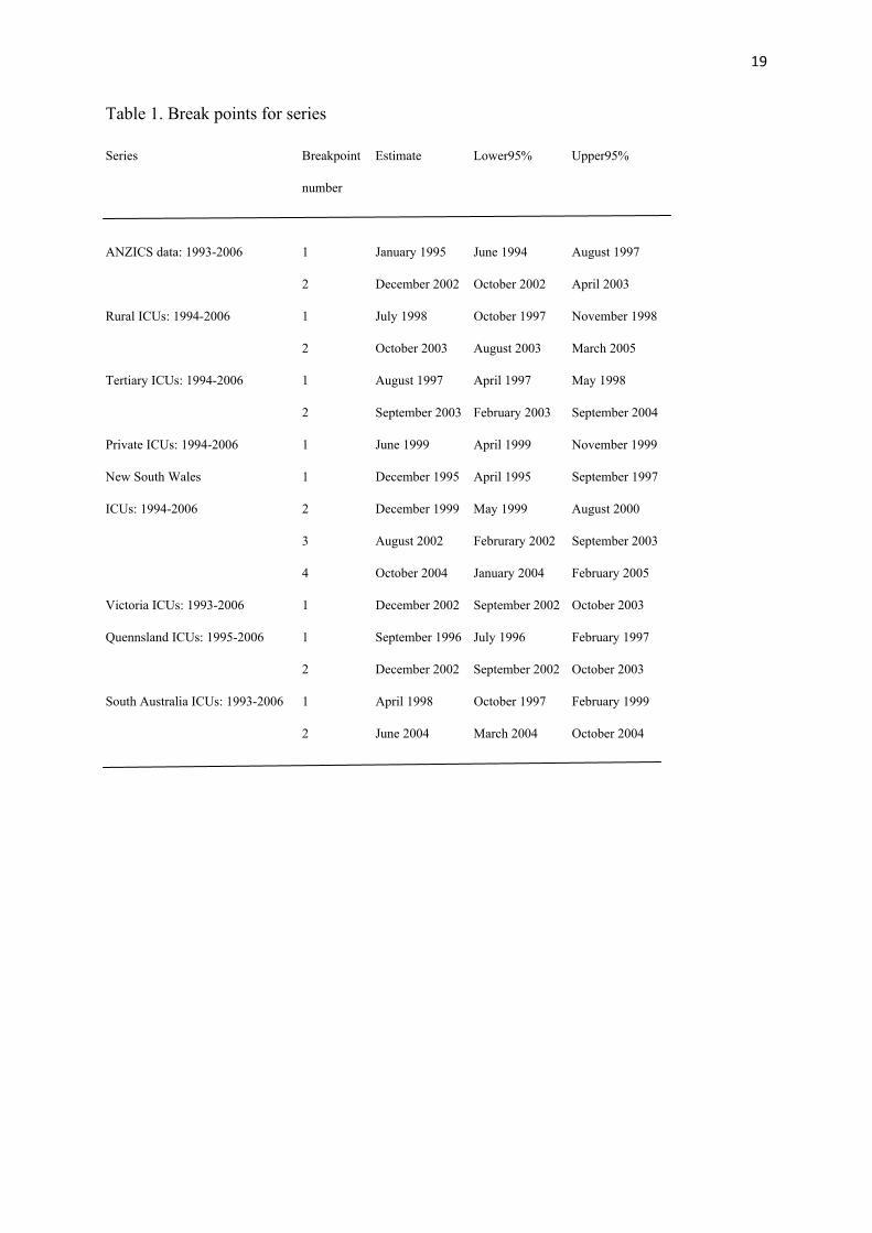
Over the whole data base, two structural breaks (Figure 3) were apparent at January 1995

(95%CI: June 1994 to August 1997) and December 2002 (95%CI: October 2002 to April

2003); no consistency was demonstrated with respect to the number or timing of structural

breaks for ICU levels (Figure 3) or geographical areas (Appendix, Figure A.2). No structural

break was identified for metropolitan ICU’s; only the Australian states of New South Wales,

Victoria, Queensland and South Australia had monthly numbers (N≥150; see Methods, Data

setup, above) in the original data-base to constitute a series of sufficient length suitable for

structural break analysis. Point estimates and 95% CI for the breaks are seen in Table 1.

10  

Decomposition of the ANZICS data-base 1993-2006 series revealed marked seasonality, a

declining mortality trend (Appendix Figure A.3) and substantial auto-correlation beyond 24

lags (Appendix, Figure A.4). Spectral density plot examination suggested dominant long-

term periodicity (annual seasonal cycle) and a low frequency cycle representing residual non-

linear decline in mortality. A stationary series (ADF test, P = 0.0001 for rejection of the null

of a unit root; Clemente-Montañés-Reyes unit-root test 59 allowing for two structural breaks: -

8.752 [critical 5% value -5.490]) was generated with first differencing, no seasonal

differencing was deemed necessary upon inspection of the appropriate series. An additive

seasonal ARIMA model was deemed the most parsimonious, as ARMA(0,1) for monthly +

ARMA(6 12 24,0) for seasonal variation: 6 6 12 12 24 24 1 1t t t t t ty y y y or

6 12 246 12 24 11 1tL L L y L using lag-operator notation, where represents first

differencing and 6 -0.156(95%CI: -0.261, -0.052; P = 0.003); 12 = 0.217(95%CI: 0.122,

0.312; P = 0.0001); 24 = 0.393(95%CI: 0.255, 0.531; P = 0.0001); and 1 -0.837(95%CI: -

0.937, -0.738; P = 0.0001). An outlier was detected at March 1993 and modelled as a “pulse”

(coefficient: 0.017(95%CI: 0.008, 0.025; P = 0.0001)); the non-significant constant was

omitted. Level shifts at January 1995, December 2002 and June 1993 were not retained in the

model (P > 0.1). Using the ‘auto.arima’ function of the R “forecast” package 70 a

(0,1,2)(2,0,0)[12] multiplicative seasonal ARIMA model was selected (minimisation of

information criterion): equivalent to 12 12 0 212,1 12,2 12 1 21 )(1 (1 )(1 )t tL L y L L ;

where 12,1 = 0.261(95%CI: 0.170, 0.352; P=0.0001); 12,2 = 0.422(0.288, 0.556; P=0.0001);

1 = -0.821(-0.961, -0.680; P=0.0001); and 2 = -0.066(-0.224, 0.092; P=0.415). Moduli of

the roots of the characteristic polynomials (both AR and MA) for both models were < 1.

Mortality predictions to a forecast horizon of 12 months (beyond December 2006) were

obtained from both models (Figure 4); formal forecast comparison (based upon mean square

error) demonstrated no statistical advantage of the additive versus the multiplicative model (P

= 0.25), albeit there was a modest BIC advantage of the former (-941.91 versus -935.94,

respectively).

The null ARCH model (dependent variable, ANZICS data-base 1993-2006 series, with a

constant term only) demonstrated significant ARCH effects. The best GARCH model was

MA(1) AR(6 12 24) ARCH(1 7) GARCH(2), including the “pulse” at March 1993 (Table 2,

“GARCH model”). There was substantial information criterion advantage compared with the

11  

additive seasonal ARIMA model (BIC -968.4 versus -941.91, respectively) and the model

was well specified by diagnostic measures 46. The mean model forecast had superior

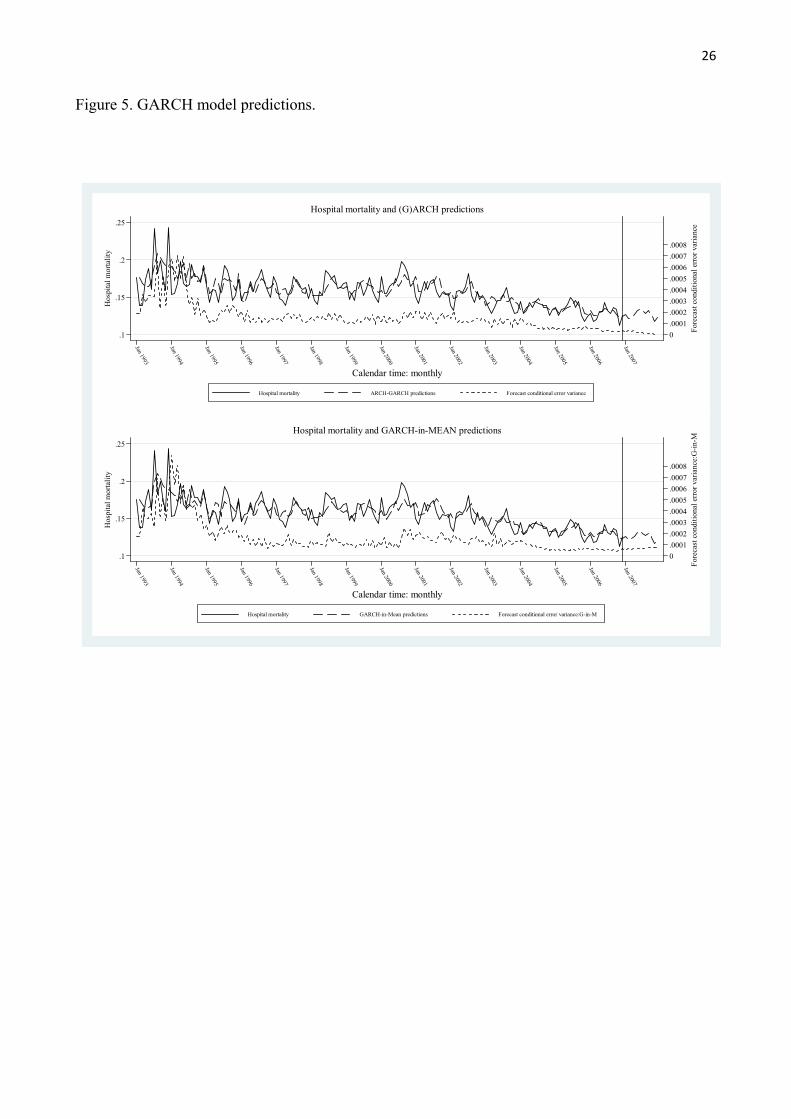
performance compared with the additive model at P=0.046 and is displayed (Figure 5, top

panel) with the conditional error variance which demonstrated a progressive decrease over

the forecast horizon. The model was re-estimated using the GARCH-in-Mean estimator

(lower panel of Figure 5), which, compared with the initial GARCH model, showed some

overall improvement in model performance (BIC -963.3 versus -968.4) but not in mean

model forecast (P = 0.21). However, the conditional error variance was projected to

increment slightly over the forecast horizon. Both GARCH models demonstrated residual

ARCH effects in the squared residuals, although this was less obvious with the GARCH-in-

Mean model.

Bivariate cointegration relationships for selected series, identified by the Engle-Granger

approach (P < 0.05 and up to lag 4 only) are shown in Table 3, suggesting stable long-term

(equilibrium) relationships. Using the autoregressive distributed lag mechanism and F-tests,

significant “Granger-causal” relationships were identified for more series compared with the

Engle-Granger approach, except for the “mortality-APACHE III score” series of the ANZICS

database 1993-2006, where no significant association was demonstrated for lags 4 through

12. Both the Bayer-Hanck 58 and Gregory-Hansen 60 approaches appeared to possess

increased sensitivity with respect to identifying significant bivariate cointegration

relationships. These relationships were further characterised by an error correction model;

specified here for the relationship between the female and male mortality series:

female_mortality 0.038 0.490 male_mortality - 0.771(female_mortality 0.613male_mortality 0.036) ,1 1 et t t where ∆ represents the differenced series.

VECM models were established for an “ICU” set (1994-2006) of series= {log APACHE III

score, log ICU length of stay (days), ICU mortality and ventilation status}, entered into the

estimation equation in the order indicated. Two cointegrating equations (with 6 lags selected)

were demonstrated and the equations were found to be stable (unit moduli < 1) and

appropriately specified; details of these cointegrating relationships are provided in Appendix

II. No statistical advantage in terms of information criterion was demonstrated for the

allowance of a quadratic trend in the undifferenced data and a linear trend in the cointegrating

equations. Impulse response functions (APACHE III score as the impulse) are seen in Figure

6 for both the orthogonal and the cumulative impulse responses. Attenuation of the

orthogonal “impulse” was variable (1-2 months); cumulative responses were sustained to 6

12  

months for ICU length-of-stay and ventilation fraction, but tended to revert at 6 months for

ICU mortality.

Discussion

We have applied a wide range of formal time-series analyses to a mortality series deriving

from a bi-national database; some of these estimators (for example, (G)ARCH 71 and VECM

models) would appear to have been utilised infrequently with biomedical series. This paucity

of use presumably reflects the known lag time of transfer of statistical technology 72 to the

biomedical literature. Our exegesis of “Statistical Methods” thus serves to highlight these

non-familiar aspects of methodology and we comment below on those features which have

concrete application.

Seasonality

The mortality seasonality of the current series (Figures A.3) was consistent with the described

seasonality of infectious diseases 73 and physiological processes underlying cardio-vascular

risk 74, as reflected in both general and cause-specific 75 winter mortality increments reported

across jurisdictions. However, population-level factors may not be determinate at the

institutional (ICU) level, where factors such as the disposition of human resources (for

example, the so-called “July-effect” relating to the influx of recently graduated doctors 76-78)

and the interplay of seasonal changes in case-mix and patient-throughput 79 may be operative.

This being said, there was not a consistent “winter” mortality effect (July through August in

the southern hemisphere) at the geographical level in the current series (Figure 2) and there

was a distinction between the periodicity of the “medical” and “surgical” series. The seasonal

mortality of the medical series was well characterised (see Results, above) and the tropical

climate of the Northern Territory (of Australia) presumably explains the lack of such

seasonality and a peak of mortality in January (Figure 2). The non-seasonal cycling of the

surgical series appears more difficult to explain, but may reflect such factors as “outliers”,

small N and the scheduling of more complex cases dependent upon human resource and

hospital-bed availability 78. The “long” period cycling observed in both medical and surgical

series is perhaps best understood as a consequence of residual non-linear trend in the (linear)

de-trended data.

Structural time-breaks

13  

Against a background of a general decline in mortality of the overall 1993-2006 series

(Figure 1), there was considerable heterogeneity in the timing, number and precision of

structural breaks in the mortality series relating to geographical- and ICU-levels. It would be

presumed that such breaks reflect (changes in) underlying patient- and institutional-

demographic and treatment factors and their interactions, as previously discussed 15.

Consistent with this proposition, a number of the series (Figures 3 and A.2) demonstrated

structural-breaks proximate (but lagged) to the publication (2000-2002) of landmark

therapeutic studies in the critically-ill 80-83, albeit the efficacy of such interventions has been

recently questioned 84,85.

Modelling the data-generating process

The data generating mechanism of the overall mortality series (1993-2006; Figure 1)

exhibited a persistent autocorrelation to at least L24 (Figure A.4) and was characterised as a

seasonal ARIMA process, similar to other mortality series 10,86-89. As in our previous report

on the ANZICS series 11, the choice between the multiplicative and additive seasonal model

was not well defined (Figure 4), although it has been suggested that “Rarely shall we need

models that incorporate autocorrelation only at the seasonal lags” 90. In the current series,

there was advantage, in terms of likelihood criterion, to the additive model. Modelling of the

error variance process constitutes an analytic initiative as both ARCH and GARCH models

were preferred compared with the ARIMA. The original motivation of the former models was

as a measure of the “risk” of a financial assets; in particular, series that exhibited volatility

clustering 17,91. The latter aspect would appear to recommend the application of (G)ARCH

models to mortality series, compared with the more conventional ARIMA,. The “volatility”

of the variance (Figure 5) in the early years of the series (1993-6) is unexplained, but may

relate to the progressive increase in the number of records contributed to the data base 15.

This being said, mortality and variance peaks extended until at least 2004, whereupon the

variance exhibited a smooth profile in both GARCH and GARCH-in-MEAN models. The

forecast decline of variance towards zero in the GARCH model (Figure 5, upper panel)

would appear to be implausible and the mild forecast variance increment of the GARCH-in-

MEAN (Figure 5, lower panel) appears more reasonable. In general, GARCH predictive

intervals reflect greater forecast uncertainty in times of high volatility 92.

The demonstration of both significant autocorrelation of the mortality series and

autoregressive heteroscedasticity of the ARIMA residuals is of some importance with respect

14  

to system control procedures (“control charts”) as applied to mortality data. Process

autocorrelation will affect the average-run-length (ARL) performance of classic CUSUM and

EWMA charts to yield false alarms 93,94. Corrective approaches have involved either

adjusting control limits 95 or the use of residual charts from a model of the process data 96,97,

the latter presuming stationary residuals. Statistical process control practitioners should thus

be mindful of residual (G)ARCH effects in auto-correlated series.

Relationships between series components

The use of cointegrating relationships to investigate long-term “equilibrium” relationships

has featured prominently in the Health Economics literature 1,98,99, but has been employed far

less frequently to answer questions pertinent to current concerns 3. The problematic nature of

modelling the time-dependence of univariate or multivariate series has been outlined above

(see Results, Statistical analysis) and has been the subject of extensive review 48,100. With

respect to a univariate series (yt) indexed by time (xt = t = 1,2,3...T), inference from

conventional linear regression 78 ( )t t ty x may be uncertain (at various levels) due

to autocorrelation of residuals 101; the effect of the latter not being ameliorated by

autocorrelation regression “correctors” 102. The demonstration, albeit in a multiple-testing

framework, of bivariate cointegration between the component series APACHE III score and

mortality (Table 3), is not surprising. As opposed to financial time series, where theory may

be lacking 103, the causality, in a strong sense, between severity-of-illness and mortality 104 is

apposite. However, the implications of a long-term equilibrium relationship (the between

male and female, ventilated and non-ventilated and medical and surgical mortality series

needs more prudent explication. Granger causality, underpinning cointegration, is predictive

in nature and it is in this sense that the cointegration of the above bivariate series should be

understood; that is, the time-course of the series does not deviate from a predictable

relationship and any tendency for this to occur is inhibited by an intrinsic “correction”

process. This being said, it is apparent that there is a certain “tangibility” to the equilibrium,

as mortality outcome derives from a complex treatment milieu which develops over time

resulting in an overall mortality decrease in the current series 15. Thus treatment regimens,

applying equally (gender) or differentially (ventilated and non-ventilated, medical and

surgical) seem, over the long term, to generate analogous outcomes.

The use of single equation residual based tests (for example, the ADF test) to establish

cointegrating relationships may be confounded by factors such as test power and sample size,

15  

and the null-hypothesis of the test, leading to “mixed signals” 105, as reflected in Table 3

where four such tests are presented.

The multivariate VECM analysis is complimentary to that of the bivariate and illustrates a

system approach to multiple cointegrating relationships (Appendix II). For a (stationary)

VAR, the I(0) variables are (by definition) mean reverting and thus the orthogonal IRFs

should revert to zero. For a VECM, this is not the case (some of the eigenvalues of the A = (k

x k) parameter matrix are 1) and, depending upon the impulse and the ordering of the

variables, the "shocks" may be transitory in effect or "permanent" 23. In the current analysis,

the APACHE III impulse was seen to generate relatively short-term effects on the other

series. Cumulative IRFs, by definition non-zero, are understood as being generated by

relatively recent shocks to the system but not those that occurred a "long" time ago. Although

we presume that the current series orderings and attendant causalities were appropriate, there

may be different IRFs with different orderings, and restrictions could also be imposed on the

coefficients (structural VECM). Thus the interpretation of an IRF must be cautious 56. With

respect to different orderings, the impulse effect of length of stay 104 and ventilation fraction 15 upon mortality could be determined at various levels of the data-base.

Critique of Methodology

The analyses were conducted at the aggregate as opposed to the individual 8 level with the

attendant inferential problems (“ecological fallacy” 106) of the former 107. The current

ARIMA approach utilised stationary series for inference and a non-linear approach, via state-

space models (which include ARMA models as a “special case” 108) could be undertaken 101.

Similarly, multivariate (G)ARCH models could be implemented, allowing volatility

comparison between geographical areas or ICU levels 109. The demonstration of structural

breaks in the series may have introduced latent bias into estimation, but we presume that the

use of unit-root and cointegration tests that accommodate the former overcame any such

tendencies. Although the GARCH-in-MEAN estimator may have appealing properties,

consistent parameter estimation requires that the full model be correctly specified, in

particular the conditional variance (other GARCH formulations may be resilient to

misspecification of the variance) 41. The residual ARCH effects noted in the current GARCH-

in-MEAN model (see Results, above), suggests cautious interpretation. The co-integration

and error-correction analysis, albeit uncommon in biomedical literature, presents a different

16  

dimension to the more familiar notions of increment of hazard or odds-ratio per unit increase

in predictor; that is, a system approach to our understanding of series time-dependence.

Conclusion

We view the application of modern time series methods on the data as highly appropriate to

investigating time-trends in Intensive Care mortality and related outcomes, with a view to

illuminating the effects of policy and the implications for policy development, and for

forecasting and prediction of mortality and other outcomes. Such recommendations

obviously extend to series from other disciplines.

17  

LEGENDS

Figure 1.

Time series plots × 4 of monthly mortality series (1993-2006) for (in clockwise order):

hospital and ICU mortality, hospital mortality by ventilation status, hospital mortality by

patient status, and hospital mortality by gender.

Figure 2.

Multiplicative seasonal mortality (normalized, reference level ≡ 1) for ANZICS database

(1993-2006) and geographical areas (New Zealand and the States of the Commonwealth of

Australia)

Figure 3.

Structural time breaks with estimate (vertical dashed lines) and 95% CI (solid capped lines),

1994-2006, for various monthly mortality series

Figure 4.

ARIMA model forecast for 12 month horizon (onset of forecast at solid vertical line) for

additive model (upper panel) and “Auto-airma” multiplicative model

Figure 5.

GARCH and GARCH-in-MEAN (mean) model forecasts (long dashed line, with forecast

onset indicated by vertical solid line); conditional error variance, short dash line.

Figure 6.

Orthogoan and cumulative impulse response functions (IRF) for ICU series (impulse log

APACHE III score). Horizontal axis, months post APACHE III impulse

Figure A.1.

Time series seasonal mortality changes (absolute scale) for years 1993-2006, by calendar

month (horizontal axis)

Figure A.2.

18  

Structural time breaks with estimate (vertical dashed lines) and 95% CI (solid capped lines),

1994-2006, for various monthly mortality series

Figure A.3.

Decomposition 25 of mortality time series (1993-2006), as observed mortality, trend, seasonal

and random effects

Figure A.4.

Mortality series autocorrelation plot 110 to lag 24; scalar estimated of correlation by panel in

box (top right hand corner of panels)

19  

Table 1. Break points for series

Series Breakpoint Estimate Lower95% Upper95%

number

ANZICS data: 1993-2006 1 January 1995 June 1994 August 1997

2 December 2002 October 2002 April 2003

Rural ICUs: 1994-2006 1 July 1998 October 1997 November 1998

2 October 2003 August 2003 March 2005

Tertiary ICUs: 1994-2006 1 August 1997 April 1997 May 1998

2 September 2003 February 2003 September 2004

Private ICUs: 1994-2006 1 June 1999 April 1999 November 1999

New South Wales 1 December 1995 April 1995 September 1997

ICUs: 1994-2006 2 December 1999 May 1999 August 2000

3 August 2002 Februrary 2002 September 2003

4 October 2004 January 2004 February 2005

Victoria ICUs: 1993-2006 1 December 2002 September 2002 October 2003

Quennsland ICUs: 1995-2006 1 September 1996 July 1996 February 1997

2 December 2002 September 2002 October 2003

South Australia ICUs: 1993-2006 1 April 1998 October 1997 February 1999

2 June 2004 March 2004 October 2004

20  

Table 2. Parameters for GARCH models

GARCH model GARCH-in-MEAN

Estimates Coefficient P value Lower 95%CI Upper 95%CI Coefficient P value Lower 95%CI Upper 95%CI

Parameter

Pulse_March 1993 0.026 0.0001 0.011 0.040 0.033 0.001 0.013 0.053

ARMA

Autoregressive

L6 -0.156 0.018 -0.284 -0.027 -0.195 0.002 -0.318 -0.073

L12 0.233 0.0001 0.109 0.358 0.212 0.001 0.085 0.339

L24 0.268 0.0001 0.150 0.385 0.269 0.0001 0.151 0.387

Moving average

L1 -0.797 0.0001 -0.894 0.385 -0.859 0.0001 -0.929 -0.779

(G)ARCH

Arch

L1 0.142 0.013 0.030 0.254 0.219 0.007 0.06 0.378

L7 -0.152 0.029 -0.289 -0.016

Garch

L2 1.025 0.0001 0.915 1.135 0.718 0.0001 0.536 0.9

ARCHM

-2.784 0.01 -4.894 -0.674

; volatility parameter of the conditional variance ( 2 ). In financial analysis, has been termed the

“coefficient of risk aversion” 43.

21  

Table 3. Bivariate cointegration relationships in selected series

ADF test P Greghansen ADL P Bayer-Hanck: P

residuals lags P lags (4 lags)

SERIES

ANZICS DATA BASE 1993-2006

Mortality: hospital & ICU -4.824 <0.01 -5.13 4 <0.01 4-12 ≥0.17 < 0.05

Mortality & APIII score

Hospital mortality & APIII score -2.085 > 0.1 -4.83 4 <0.025 4-12 ≤ 0.02 < 0.05

ICU mortality & APIII score -2.31 > 0.2 -4.66 4 <0.05 4-12 < 0.04 < 0.05

Ventilation staus & mortality

Hospital: ventilated & non-ventilated -1.796 > 0.1 -6.09 2 <0.01 4-8 ≤0.05 < 0.05

ICU: ventilated & non-ventilated -2.445 > 0.1 -5.12 3 <0.025 10-12 ≤0.05 < 0.05

Gender&mortality: male & female -4.885 < 0.01 -6.16 4 < 0.01 4-12 ≤0.0001 < 0.05

Patient type& mortality

surgical & non-surgical -3.797 < 0.01 -4.53 4 <0.1 6-12 ≤0.05 < 0.05

RURAL ICUs 1994-2006

Mortality & APIII score -2.729 > 0.1 -5.15 4 <0.01 4-12 > 0.4 < 0.05

METROPOLITAN ICUs 1994-2006

Mortality & APIII score -6.453 < 0.01 -7.35 4 <0.01 4-12 < 0.005 < 0.05

TERTIARY ICUs 1994-2006

Mortality & APIII score -1.784 >0.1 -4.78 3 <0.05 4-12 >0.63 > 0.05

PRIVATE ICUs 1994-2006

Mortality & APIII score -3.629 <0.05 -5.72 4 <0.01 4-12 <0.002 < 0.05

ADF test; augmented Dickey-Fuller test on residuals of bivariate least squares regressions. Critical values

(Engle&Granger 1987 49) for ADF are: 1%: 3.77; 5%: 3.17; 10%: 2.84. Greghansen; Gregory-Hansen test for

cointegration; level-shift structural change, lags ≤4 .ADL60; autoregressive distributed lag relationships between

bivariate series 55. Lags; number of lags considered. Bayer-Hanck combination test.58 #: P ≤ 0.05 for lags 1&2.

22  

Figure 1. Monthly mortality series

0

.05

.1

.15

.2

.25

.3

.35

Mor

talit

y fr

actio

n

Jan 1993

Jan 1994

Jan 1995

Jan 1996

Jan 1997

Jan 1998

Jan 1999

Jan 2000

Jan 2001

Jan 2002

Jan 2003

Jan 2004

Jan 2005

Jan 2006

Calendar time: monthly

Hospital mortality ICU mortality

Monthly hospital & ICU mortality: 1993-2006

0

.05

.1

.15

.2

.25

.3

.35

Mor

talit

y fr

actio

n

Jan 1993

Jan 1994

Jan 1995

Jan 1996

Jan 1997

Jan 1998

Jan 1999

Jan 2000

Jan 2001

Jan 2002

Jan 2003

Jan 2004

Jan 2005

Jan 2006

Calendar time: monthly

Hospital mortality: ventilated Hospital mortality: non-ventilated

Monthly hospital mortality, by ventilation status: 1993-2006

0

.05

.1

.15

.2

.25

.3

.35

Mor

talit

y fr

actio

n

Jan 1993

Jan 1994

Jan 1995

Jan 1996

Jan 1997

Jan 1998

Jan 1999

Jan 2000

Jan 2001

Jan 2002

Jan 2003

Jan 2004

Jan 2005

Jan 2006

Calendar time: monthly

Hospital mortality: medical Hospital mortality: surgical

Monthly hospital mortality, by patient type: 1993-2006

0

.05

.1

.15

.2

.25

.3

.35

Mor

talit

y fr

actio

n

Jan 1993

Jan 1994

Jan 1995

Jan 1996

Jan 1997

Jan 1998

Jan 1999

Jan 2000

Jan 2001

Jan 2002

Jan 2003

Jan 2004

Jan 2005

Jan 2006

Calendar time: monthly

Hospital mortality: male Hospital mortality: female

Monthly hospital mortality, by Gender: 1993-2006

23  

Figure 2. Seasonal mortality for the ANZICS data base and geographical areas

.8

.9

1

1.1

1.2

1.3

Nor

mal

ized

sea

sona

l mor

talit

y

JanFebM

arA

prM

ayJunJulA

ugSepO

ctN

ovD

ec

Calendar time: months

Whole database

.8

.9

1

1.1

1.2

1.3

Nor

mal

ized

sea

sona

l mor

talit

y

JanFebM

arA

prM

ayJunJulA

ugSepO

ctN

ovD

ec

Calendar time: months

Northern Territory

.8

.9

1

1.1

1.2

1.3

Nor

mal

ized

sea

sona

l mor

talit

y

JanFebM

arA

prM

ayJunJulA

ugSepO

ctN

ovD

ec

Calendar time: months

Victoria

.8

.9

1

1.1

1.2

1.3

Nor

mal

ized

sea

sona

l mor

talit

y

JanFebM

arA

prM

ayJunJulA

ugSepO

ctN

ovD

ec

Calendar time: months

Queensland

.8

.9

1

1.1

1.2

1.3

Nor

mal

ized

sea

sona

l mor

talit

y

JanFebM

arA

prM

ayJunJulA

ugSepO

ctN

ovD

ec

Calendar time: months

Tasmania

.8

.9

1

1.1

1.2

1.3

Nor

mal

ized

sea

sona

l mor

talit

y

JanFebM

arA

prM

ayJunJulA

ugSepO

ctN

ovD

ec

Calendar time: months

New South Wales

.8

.9

1

1.1

1.2

1.3

Nor

mal

ized

sea

sona

l mor

talit

y

JanFebM

arA

prM

ayJunJulA

ugSepO

ctN

ovD

ec

Calendar time: months

South Australia

.8

.9

1

1.1

1.2

1.3

Nor

mal

ized

sea

sona

l mor

talit

y

JanFebM

arA

prM

ayJunJulA

ugSepO

ctN

ovD

ec

Calendar time: months

New Zealand

.8

.9

1

1.1

1.2

1.3

Nor

mal

ized

sea

sona

l mor

talit

y

JanFebM

arA

prM

ayJunJulA

ugSepO

ctN

ovD

ec

Calendar time: months

ACT

24  

Figure 3. Structural time breaks for series: ANZICS data base and ICU levels

ANZICS database: 1993-2006

Calendar time: monthly

Hos

pita

l mor

talit

y

1994 1998 2002 2006

0.00

0.05

0.10

0.15

0.20

0.25

Rural ICUs: 1994-2006

Calendar time: monthly

Hos

pita

l mor

talit

y

1994 1998 2002 2006

0.00

0.05

0.10

0.15

0.20

0.25

Tertiary ICUs: 1993-2006

Calendar time: monthly

Hos

pita

l mor

talit

y

1994 1998 2002 2006

0.00

0.05

0.10

0.15

0.20

0.25

Private ICUs: 1994-2006

Calendar time: monthly

Hos

pita

l mor

talit

y

1994 1998 2002 2006

0.00

0.05

0.10

0.15

0.20

0.25

25  

Figure 4. ARIMA model predictions

.05

.1

.15

.2

.25

Jan 1993

Jan 1994

Jan 1995

Jan 1996

Jan 1997

Jan 1998

Jan 1999

Jan 2000

Jan 2001

Jan 2002

Jan 2003

Jan 2004

Jan 2005

Jan 2006

Jan 2007

Calendar time: monthly

Hospital mortality Additive model predictions Upper 95%CI Lower 95%CI

Hospital mortality and additive model predictions

.05

.1

.15

.2

.25

Jan 1993

Jan 1994

Jan 1995

Jan 1996

Jan 1997

Jan 1998

Jan 1999

Jan 2000

Jan 2001

Jan 2002

Jan 2003

Jan 2004

Jan 2005

Jan 2006

Jan 2007

Calendar time: monthly

Hospital mortality Auto-arima predictions Upper 95%CI Lower 95%CI

Hospital mortality and Auto-arima predictions

26  

Figure 5. GARCH model predictions.

0

.0001

.0002

.0003

.0004

.0005

.0006

.0007

.0008

Fore

cast

con

diti

onal

err

or v

aria

nce

.1

.15

.2

.25

Hos

pita

l mor

tali

ty

Jan 1993

Jan 1994

Jan 1995

Jan 1996

Jan 1997

Jan 1998

Jan 1999

Jan 2000

Jan 2001

Jan 2002

Jan 2003

Jan 2004

Jan 2005

Jan 2006

Jan 2007

Calendar time: monthly

Hospital mortality ARCH-GARCH predictions Forecast conditional error variance

Hospital mortality and (G)ARCH predictions

0

.0001

.0002

.0003

.0004

.0005

.0006

.0007

.0008

Fore

cast

con

diti

onal

err

or v

aria

nce:

G-i

n-M

.1

.15

.2

.25

Hos

pita

l mor

tali

ty

Jan 1993

Jan 1994

Jan 1995

Jan 1996

Jan 1997

Jan 1998

Jan 1999

Jan 2000

Jan 2001

Jan 2002

Jan 2003

Jan 2004

Jan 2005

Jan 2006

Jan 2007

Calendar time: monthly

Hospital mortality GARCH-in-Mean predictions Forecast conditional error variance:G-in-M

Hospital mortality and GARCH-in-MEAN predictions

27  

Figure 6. IRF for ICU series

28  

Appendix

Figure A.1. Seasonal plot for ANZICS database series

0.12

0.14

0.16

0.18

0.20

0.22

0.24

ANZICS database: 1993-2006

Month

Ho

spita

l mo

rta

lity

1993

1994

1995

1996

1997

1998

1999

2000

20012002

2003

2004

20052006

Jan Feb Mar Apr May Jun Jul Aug Sep Oct Nov Dec

29  

Figure A.2. Structural time breaks for series of geographical areas

NSW: 1994-2006

Calendar time: monthly

Hos

pita

l mor

talit

y

1994 1998 2002 2006

0.05

0.10

0.15

0.20

0.25

0.30

0.35

Victoria: 1994-2006

Calendar time: monthly

Hos

pita

l mor

talit

y1994 1998 2002 2006

0.05

0.10

0.15

0.20

0.25

0.30

0.35

Queensland: 1995-2006

Calendar time: monthly

Hos

pita

l mor

talit

y

1996 2000 2004

0.05

0.10

0.15

0.20

0.25

0.30

0.35

South Australia: 1995-2006

Calendar time: monthly

Hos

pita

l mor

talit

y

1996 2000 2004

0.05

0.10

0.15

0.20

0.25

0.30

0.35

30  

Figure A.3. Decomposition of the ANZICS database series (1993-2006)

31  

Figure A.4. ANZICS series autocorrelation via lag-plot 110.

0.12 0.18 0.24

0.12

0.20

Anzics.series(t-1)

Anz

ics.

serie

s(t)

0.59

0.12 0.18 0.24

0.12

0.20

Anzics.series(t-2)

Anz

ics.

serie

s(t)

0.51

0.12 0.18 0.24

0.12

0.20

Anzics.series(t-3)

Anz

ics.

serie

s(t)

0.49

0.12 0.18 0.24

0.12

0.20

Anzics.series(t-4)

Anz

ics.

serie

s(t)

0.44

0.12 0.18 0.24

0.12

0.20

Anzics.series(t-5)

Anz

ics.

serie

s(t)

0.39

0.12 0.18 0.24

0.12

0.20

Anzics.series(t-6)

Anz

ics.

serie

s(t)

0.3

0.12 0.18 0.24

0.12

0.20

Anzics.series(t-7)

Anz

ics.

serie

s(t)

0.35

0.12 0.18 0.24

0.12

0.20

Anzics.series(t-8)

Anz

ics.

serie

s(t)

0.43

0.12 0.18 0.24

0.12

0.20

Anzics.series(t-9)

Anz

ics.

serie

s(t)

0.38

0.12 0.18 0.24

0.12

0.20

Anzics.series(t-10)

Anz

ics.

serie

s(t)

0.35

0.12 0.18 0.24

0.12

0.20

Anzics.series(t-11)

Anz

ics.

serie

s(t)

0.48

0.12 0.18 0.24

0.12

0.18

Anzics.series(t-12)

Anz

ics.

serie

s(t)

0.49

0.12 0.18 0.24

0.12

0.18

Anzics.series(t-13)

Anz

ics.

serie

s(t)

0.4

0.14 0.20

0.12

0.18

Anzics.series(t-14)

Anz

ics.

serie

s(t)

0.29

0.14 0.20

0.12

0.18

Anzics.series(t-15)

Anz

ics.

serie

s(t)

0.32

0.14 0.20

0.12

0.18

Anzics.series(t-16)

Anz

ics.

serie

s(t)

0.25

0.14 0.20

0.12

0.18

Anzics.series(t-17)

Anz

ics.

serie

s(t)

0.18

0.14 0.20

0.12

0.18

Anzics.series(t-18)

Anz

ics.

serie

s(t)

0.18

0.14 0.20

0.12

0.18

Anzics.series(t-19)

Anz

ics.

serie

s(t)

0.21

0.14 0.200.

120.

18

Anzics.series(t-20)

Anz

ics.

serie

s(t)

0.24

0.14 0.20

0.12

0.18

Anzics.series(t-21)

Anz

ics.

serie

s(t)

0.26

0.14 0.20

0.12

0.18

Anzics.series(t-22)

Anz

ics.

serie

s(t)

0.26

0.14 0.20

0.12

0.18

Anzics.series(t-23)

Anz

ics.

serie

s(t)

0.34

0.14 0.20

0.12

0.18

Anzics.series(t-24)

Anz

ics.

serie

s(t)

0.39

32  

Appendix II

VECM cointegrating relationships for the ICU series set:

(1) ln(APIII score) 1.261 (ICU.mortality) 0.435 (ventilation.fraction) 3.887t t t tc , where the

coefficient of ln(APACHE III score) is constrained to unity and that of log(ICU length-of-stay) to

zero

and

(2) ln(ICU.los) 1.233 (ICU.mortality) 0.893 (ventilation.fraction) 0.996t t t tc , where the

coefficient of log(ICU length-of-stay) is constrained to unity and that of log(APACHE III score) to

zero.

33  

Literature Cited

1. Bishai,D.M. (1995) Infant mortality time series are random walks with drift: Are they

cointegrated with socioeconomic variables? Health Economics, 4(3), 157-167.

2. Helfenstein,U. (1990) Detecting hidden relations between time series of mortality

rates. Methods Inf.Med, 29(1), 57-60.

3. Mills,T.C. (2007) Liver cirrhosis and alcohol consumption in the U.K.: time series

modelling of recent trends. Statistical Modelling, 7(1), 91-103.

4. Peng,R.D. 7 F. Dominici. (2008) Statistical Methods for Environmental

Epidemiology with R. Springer Science+Business Media, LLC, New York, NY.

5. Zhang,F., Wagner,A.K., Soumerai,S.B. & Ross-Degnan,D. (2009) Methods for

estimating confidence intervals in interrupted time series analyses of health

interventions. Journal of Clinical Epidemiology, 62(2), 143-148.

6. Harbarth,S. & Samore,M.H. (2008) Interventions to control MRSA: high time for

time-series analysis? Journal of Antimicrobial Chemotherapy, 62(3), 431-433.

7. Smith,D.H., Perrin,N., Feldstein,A.et al. (2006) The Impact of Prescribing Safety

Alerts for Elderly Persons in an Electronic Medical Record: An Interrupted Time

Series Evaluation. Archives of Internal Medicine, 166(10), 1098-1104.

34  

8. Crabtree,B.F., Ray,S.C., Schmidt,P.M., O'Connor,P.T. & Schmidt,D.D. (1990) The

individual over time: Time series applications in health care research. Journal of

Clinical Epidemiology, 43(3), 241-260.

9. Gillings,D., Makuc,D. & Siegel,E. (1981) Analysis of interrupted time series

mortality trends: an example to evaluate regionalized perinatal care. American

Journal of Public Health, 71(1), 38-46.

10. Zeger,S.L., Irizarry,R. & Peng,R.D. (2006) On time series analysis of public health

and biomedical data. Annual Review of Public Health, 27:57-79.

11. Moran,J.L. & Solomon,P.J. (2007) Statistics in Review. Part 2: Generalised linear

models, time-to-event and time-series analysis, eveidence synthesis and clinical trials.

Critical Care and Resuscitation, 9(2), 187-197.

12. Helfenstein,U. (1996) Box-Jenkins modelling in medical research. Statistical Methods

in Medical Research, 5(1), 3-22.

13. Stow,P.J., Hart,G.K., Higlett,T.et al. (2006) Development and implementation of a

high-quality clinical database: the Australian and New Zealand Intensive Care Society

Adult Patient Database. Journal of Critical Care, 21(2), 133-141.

14. Wooldridge, J. M. (2000) Basic regression analysis with time series data. In:

Wooldridge, J. M., editors. Introductory econometrics: A modern approach. South-

Western College Publishing.

35  

15. Moran,J.L., Bristow,P., Solomon,P.J.et al. (2008) Mortality and length-of-stay

outcomes, 1993-2003, in the binational Australian and New Zealand intensive care

adult patient database. Critical Care Medicine, 36(1), 46-61.

16. Gould,P.G., Koehler,A.B., Ord,J.K.et al. (2008) Forecasting time series with multiple

seasonal patterns. European Journal of Operational Research, 191(1), 207-222.

17. Engle,R. (2001) GARCH 101: The Use of ARCH/GARCH Models in Applied

Econometrics. The Journal of Economic Perspectives, 15(4), 157-168.

18. Lutkepohl,H. (2005) New Introduction to Multiple Time Series Analysis. 2nd ed.

Springer-Verlag, Berlin.

19. Pfaff,B. (2009) Analysis of Integrated and Cointegrated Time Series with R. 2nd ed.

Springer Science+Business Media, LLC, New York, NY.

20. Walls,T.A. 7 J. L. Shafer. (2006) Models for Intensive Longitudinal data. Oxfrod

University Press, Inc, New York, NY.

21. Choudhury,A.H., Hubata,R. & Louis,R.D.S. (1999) Understanding Time-Series

Regression Estimators. The American Statistician, 53(4), 342-348.

22. Knaus,W.A., Wagner,D.P., Draper,E.A.et al. (1991) The APACHE III prognostic

system. Risk prediction of hospital mortality for critically ill hospitalized adults.

Chest, 100(6), 1619-1636.

36  

23. Stata Corp. (2009) Time Series Manual: Release 11. StataCorp LP, College Station,

TX.

24. Ihaka,R. & Gentleman,R. (/9) R: A Language for Data Analysis and Graphics.

Journal of Computational and Graphical Statistics, 5(3), 299-314.

25. Shiskin,J. (1958) Decomposition of Economic Time Series. Science, 128(3338),

1539-1546.

26. Archibald,B.C. & Koehler,A.B. (2003) Normalization of seasonal factors in Winters'

methods. International Journal of Forecasting, 19(1), 143-148.

27. Bai,J. & Perron,P. (2003) Computation and Analysis of Multiple Structural Change

Models. Journal of Applied Econometrics, 18(1), 1-22.

28. Zeileis,A., Leisch,F., Hornik,K. & Kleiber,C. (2002) strucchange: An R Package for

Testing for Structural Change in Linear Regression Models. Journal of Statistical

Software, 7(2), 1-38.

29. Commandeur, J. J. & Koopman, S. J. (2007) State space and Box-Jenkins methods for

time series analysis. In: Commandeur, J. J. & Koopman, S. J., editors. An introduction

to Stata Space Series Analysis. 122-134. Oxford, UK: Oxford University Press.

30. Shumway,R.H. & Stoffer,D.S. (2009) Some R Time Series Issues. @

http://www.stat.pitt.edu/stoffer/tsa2/Rissues.htm, Accessed May 2009.

37  

31. Diebold, F. X. (2001) Modeling cycles: MA, AR, and ARMA models. In: Diebold, F.

X., editors. Elements of forecasting. 2nd ed. pp.143-182. Cincinati, Ohio: South-

Western.

32. Venables, W. N. & Ripley, B. D. (2006) Time series analysis. In: Venables, W. N. &

Ripley, B. D., editors. Modern applied statistics with S. 4th Edition ed. pp.387-418.

New York: Springer-Verlag New York, Inc.

33. Kuha,J. (2004) AIC and BIC: Comparisons of Assumptions and Performance.

Sociological Methods Research, 33(2), 188-229.

34. Tsay,R.S. (1988) Outliers, Level Shifts, and Variance Changes in Time Series.

Journal of Forecasting, 7(1), 1-20.

35. Balke,N.S. (1993) Detecting Level Shifts in Time Series. Journal of Business &

Economic Statistics, 11(1), 81-92.

36. Cryer, J. D. & Chan, K.-S. (2008) Model diagnostics. In: Cryer, J. D. & Chan, K.-S.,

editors. Time Series Analysis With Applications in R. 2nd ed. pp.175-190. New York,

NY: Springer Science+Business Media, LLC.

37. Baum,C. (2009) dmariano: Stata module to compute Diebold-Mariano comparison of

predictive accuracy. @ http://econpapers.repec.org/scripts/search.asp?ft=dmariano.

38. Hyndman,R.J. & Koehler,A.B. (2006) Another look at measures of forecast accuracy.

International Journal of Forecasting, 22(4), 679-688.

38  

39. Heiberger, R. M. & Holland, B. (2004) Time Series Analysis. In: Heiberger, R. M. &

Holland, B., editors. Statistical Analysis and Data Display. An Intermediate Course

with Examples in S-Plus, R, and SAS. 565-622. New York: Springer Science

+Business Media Inc.

40. Bollerslev,T. (1986) Generalized autoregressive conditional heteroskedasticity.

Journal of Econometrics, 31(3), 307-327.

41. Bollerslev,T., Chou,R.Y. & Kroner,K.F. (1992) ARCH modeling in finance : A

review of the theory and empirical evidence. Journal of Econometrics, 52(1-2), 5-59.

42. Engle,R.F., Lilien,D.M. & Robins,R.P. (1987) Estimating Time Varying Risk Premia

in the Term Structure: The Arch-M Model. Econometrica, 55(2), 391-407.

43. Greene, W. H. (2003) Heteroscedasticity. In: Greene, W. H., editors. Econometric

Analysis. 5th ed. pp.215-249. Upper Saddle River, NJ: Prentice-Hall, Inc.

44. Politis,D.N. (2003) The Impact of Bootstrap Methods on Time Series Analysis.

Statistical Science, 18(2), 219-230.

45. Milhoj,A. (1985) The Moment Structure of ARCH Processes. Scandinavian Journal

of Statistics, 12(4), 281-292.

46. Karlsson,S. (2009) ARMADIAG: Stata module to compute post-estimation residual

diagnostics for time series. @

http://econpapers.repec.org/scripts/search.asp?ft=armadiag, Accessed, May 2009.

39  

47. Banerjee, A., Dolado, J., Galbraith, J. W., & Hendry, D. F. (1993) Properties of

integrated processes. In: Banerjee, A., Dolado, J., Galbraith, J. W., & Hendry, D. F.,

editors. Co-Integration, Error-Correction, and The Econometric Analysis of Non-

Stationary Data. 136-161. Oxford, UK: Oxford University Press.

48. Granger,C.W.J. & Newbold,P. (1974) Spurious regressions in econometrics. Journal

of Econometrics, 2(2), 111-120.

49. Engle,R.F. & Granger,C.W.J. (1987) Co-Integration and Error Correction:

Representation, Estimation, and Testing. Econometrica, 55(2), 251-276.

50. Banerjee, A., Dolado, J., Galbraith, J. W., & Hendry, D. F. (1993) Co-integration. In:

Banerjee, A., Dolado, J., Galbraith, J. W., & Hendry, D. F., editors. Co-Integration,

Error-Correction, and The Econometric Analysis of Non-Stationary Data. 136-161.

Oxford, UK: Oxford University Press.

51. Phillips,P.C.B. & Xiao,Z. (1998) A Primer on Unit Root Testing. Journal of

Economic Surveys, 12(5), 423-470.

52. Banerjee, A., Dolado, J., Galbraith, J. W., & Hendry, D. F. (1993) Linear

transformations, Error Correction, and the Long Run in Dynamic regression. In:

Banerjee, A., Dolado, J., Galbraith, J. W., & Hendry, D. F., editors. Co-Integration,

Error-Correction, and The Econometric Analysis of Non-Stationary Data. 46-68.

Oxford, UK: Oxford University Press.

40  

53. Pfaff, B. (2009) Concept of Cointegration and Error-correction Models. In: Pfaff, B.,

editors. Analysis of Integrated and Cointegrated Time Series with R. 2nd ed. pp.73-

87. New York, NY: Springer Science+Business Media, LLC.

54. Granger,C.W.J. (1969) Investigating Causal Relations by Econometric Models and

Cross-spectral Methods. Econometrica, 37(3), 424-438.

55. Joly,P. (2009) GCAUSE: Stata module to perform Granger causality tests.

http://econpapers.repec.org/scripts/search.asp?ft=gcause, Accessed May 2009.

56. Lutkepohl, H. (2005) Stable Vector Autoregressive Processes. In: Lutkepohl, H.,

editors. New Introduction to Multiple Time Series Analysis. 2nd ed. pp.13-68. Berlin:

Springer-Verlag.

57. Petris, G., Petrone, S., & Campagnoli, P. (2009) Model specification. In: Petris, G.,

Petrone, S., & Campagnoli, P., editors. Dynamic Linear models with R. 85-142.

Dordrecht: Springer Science + Business Media, LLC.

58. Bayer,C. & Hanck,C. (2009) Combining Non-Cointegration Tests. @

http://ideas.repec.org/p/dgr/umamet/2009012.html, Accessed June 2009.

59. Clemente,J., Montanes,A. & Reyes,M. (1998) Testing for a unit root in variables with

a double change in the mean. Economics Letters, 59(2), 175-182.

60. Gregory,A.W. & Hansen,B.E. (1996) Residual-based tests for cointegration in models

with regime shifts. Journal of Econometrics, 70(1), 99-126.

41  

61. Poi,B. (2009) greghansen: Stata module to implement the Gregory-Hansen test for

cointegration in models with regime shifts. User-written command: Send an email to

bpoi@stata.com to obtain the current version, Accessed July 2009.

62. Holden,K. (1995) Vector Autoregression Modelling and Forecasting. Journal of

Forecasting, 14(3), 159-166.

63. Sims,C.A., Stock,J.H. & Watson,M.W. (1990) Inference in Linear Time Series

Models with some Unit Roots. Econometrica, 58(1), 113-144.

64. Robertson, D. & Wickens.M. (1994) VAR modelling. In: Robertson, D. &

Wickens.M., editors. Applied Economic Forecasting Techniques. 29-47. Hemel

Hempstead: Harvester Wheatsheaf.

65. Gonzalo,J. (1994) Five alternative methods of estimating long-run equilibrium

relationships. Journal of Econometrics, 60(1-2), 203-233.

66. Lutkepohl, H. (2005) Vector error correction models. In: Lutkepohl, H., editors. New

Introduction to Multiple Time Series Analysis. 2nd ed. pp.237-267. Berlin: Springer-

Verlag.

67. Pfaff,B. (2008) VAR, SVAR and SVEC Models: Implementation Within R Package

vars. Journal of Statistical Software, 27(4), 1-32.

68. Pesaran,H. & Smith,R.P. (1998) Structural Analysis of Cointegrating VARs. Journal

of Economic Surveys, 12(5), 471-505.

42  

69. Stock,J.H. & Watson,M.W. (2001) Vector Autoregressions. The Journal of Economic

Perspectives, 15(4), 101-115.

70. Hyndman,R.J. & Khandakar,Y. (2008) Automatic Time Series Forecasting: The

forecast Package for R. Journal of Statistical Software, 27(3), 1-22.

71. Hu,M.Y. & Tsoukalas,C. (2006) Conditional volatility properties of sleep-disordered

breathing. Computers in Biology and Medicine, 36(3), 303-312.

72. Altman,D.G. & Goodman,S.N. (1994) Transfer of technology from statistical journals

to the biomedical literature. Past trends and future predictions. JAMA, 272(2), 129-

132.

73. Fisman,D.N. (2007) Seasonality of Infectious Diseases. Annual Review of Public

Health, 28(1), 127-143.

74. Gemmell,I., McLoone,P., Boddy,F.A., Dickinson,G.J. & Watt,G.C.M. (2000)

Seasonal variation in mortality in Scotland. International Journal of Epidemiology,

29(2), 274-279.

75. van Rossum,C.T., Shipley,M.J., Hemingway,H.et al. (2001) Seasonal variation in

cause-specific mortality: Are there high-risk groups? 25-year follow-up of civil

servants from the first Whitehall study. International Journal of Epidemiology, 30(5),

1109-1116.

43  

76. Barry,W. & Rosenthal,G. (2003) Is there a July Phenomenon? Journal of General

Internal Medicine, 18(8), 639-645.

77. Claridge,J.A., Schulman,A.M., Sawyer,R.G., Ghezel-Ayagh,A. & Young,J.S. (2001)

The "July phenomenon" and the care of the severely injured patient: Fact or fiction?

Surgery, 130(2), 346-353.

78. Englesbe,M.J.M., Pelletier,S.J.M., Magee,J.C.M.et al. (2007) Seasonal Variation in

Surgical Outcomes as Measured by the American College of Surgeons-National

Surgical Quality Improvement Program (ACS-NSQIP). Annals of Surgery, 246(3),

456-465.

79. Harrison,D., Lertsithichai,P., Brady,A., Carpenter,J. & Rowan,K. (2004) Winter

excess mortality in intensive care in the UK: an analysis of outcome adjusted for

patient case mix and unit workload. Intensive Care Medicine, 30(10), 1900-1907.

80. Annane,D., Sebille,V., Charpentier,C.et al. (2002) Effect of treatment with low doses

of hydrocortisone and fludrocortisone on mortality in patients with septic shock.

JAMA., 288(7), 862-871.

81. Bernard,G.R., Vincent,J.L., Laterre,P.F.et al. (2001) Efficacy and safety of

recombinant human activated protein C for severe sepsis. New England Journal of

Medicine, 344(10), 699-709.

82. The ARDS Network Authors for the ARDS Network. (2000) Ventilation with lower

tidal volumes as compared with traditional tidal volumes for acute lung injury and the

44  

acute respiratory distress syndrome. The Acute Respiratory Distress Syndrome

Network. New England Journal of Medicine, 342(18), 1301-1318.

83. Van den Berghe,G., Wouters,P., Weekers,F.et al. (2001) Intensive insulin therapy in

the critically ill patients. New England Journal of Medicine, 345(19), 1359-1367.

84. Annane,D., Bellissant,E., Bollaert,P.E.et al. (2009) Corticosteroids in the Treatment

of Severe Sepsis and Septic Shock in Adults: A Systematic Review. JAMA, 301(22),

2362-2375.

85. The NICE-SUGAR Study Investigators. (2009) Intensive versus Conventional

Glucose Control in Critically Ill Patients. The New England Journal of Medicine,

360(13), 1283-1297.

86. Choi,K.E. & Thacker,S.B. (1981) An evaluation of influenza mortality surveillance,

1962-1979: I. Time series forecasts of expected pneumonia and influenza deaths.

American Journal of Epidemiology, 113(3), 215-226.

87. Kis,M. (2002) Analysis of the time series for some causes of death. Studies in Health

Technology and Informatics, 90:439-443.

88. Kis,M. (2005) Time series models on analysing mortality rates and acute childhood

lymphoid leukaemia. Studies in Health Technology and Informatics, 116:15-20.

89. Norstrom,T. & Ramstedt,M. (2005) Mortality and population drinking: a review of

the literature. Drug & Alcohol Review, 24(6), 537-547.

45  

90. Cryer, J. D. & Chan, K.-S. (2008) Seasonal models. In: Cryer, J. D. & Chan, K.-S.,

editors. Time Series Analysis With Applications in R. 2nd ed. pp.227-248. New York,

NY: Springer Science+Business Media, LLC.

91. Engle,R. (2002) New Frontiers for Arch Models. Journal of Applied Econometrics,

17(5), 425-446.

92. Lutkepohl, H. (2005) Multivariate ARCH and GARCH models. In: Lutkepohl, H.,

editors. New Introduction to Multiple Time Series Analysis. 557-584. Berlin:

Springer-Verlag.

93. Alwan,L.C. (1992) Effects of autocorrelation on control chart performance.

Communications in Statistics - Theory and Methods, 21(4), 1025-1049.

94. Winkel, P. & Zhang, N. F. (2009) Control charts for autocrrelated data. In: Winkel, P.

& Zhang, N. F., editors. Statistical development of Quality in Medicine. 92-109.

Chichester, West Sussex: John Wiley & Sons Ltd.

95. Zhang,N.F. (/2) A Statistical Control Chart for Stationary Process Data.

Technometrics, 40(1), 24-38.

96. Apley,D.W. & Lee,H.C. (2008) Robustness Comparison of Exponentially Weighted

Moving-Average Charts on Autocorrelated Data and on Residuals. Journal of Quality

Technology, 40(4), 428-427.

46  

97. Apley,D.W. & Lee,H.C. (2003) Design of exponentially weighted moving average

control charts for autocorrelated processes with model uncertainty. Technometrics,

45(3), 187.

98. Hansen,P. & King,A. (1996) The determinants of health care expenditure: A

cointegration approach. Journal of Health Economics, 15(1), 127-137.

99. Okunade,A.A. & Murthy,V.N.R. (2002) Technology as a `major driver' of health care

costs: a cointegration analysis of the Newhouse conjecture. Journal of Health

Economics, 21(1), 147-159.

100. Nelson,C.R. & Kang,H. (1984) Pitfalls in the Use of Time as an Explanatory Variable

in Regression. Journal of Business & Economic Statistics, 2(1), 73-82.

101. Commandeur,J.J. 7 S. J. Koopman. (2007) An introduction to Stata Space Series

Analysis. Oxford University Press, Oxford, UK.

102. Mizon,G.E. (1995) A simple message for autocorrelation correctors: Don't. Journal of

Econometrics, 69(1), 267-288.

103. Nelson,C.R. & Plosser,C.R. (1982) Trends and random walks in macroeconmic time

series : Some evidence and implications. Journal of Monetary Economics, 10(2), 139-

162.

47  

104. Knaus,W.A., Wagner,D.P., Zimmerman,J.E. & Draper,E.A. (1993) Variations in

mortality and length of stay in intensive care units. Annals of Internal Medicine.,

118(10), 753-761.

105. Gregory,A.W., Haug,A.A. & Lomuto,N. (2004) Mixed signals among tests for

cointegration. Journal of Applied Econometrics, 19(1), 89-98.

106. Kramer,G.H. (/3) The Ecological Fallacy Revisited: Aggregate- versus Individual-

level Findings on Economics and Elections, and Sociotropic Voting. The American

Political Science Review, 77(1), 92-111.

107. Norstrom,T. & Skrog,O.-L. (2001) Alcohol and mortality: methodological and

analytical issues in aggregate analyses. Addiction, 96(1s1), 5-17.

108. Petris,G., S. Petrone, & P. Campagnoli. (2009) Dynamic Linear models with R.

Springer Science + Business Media, LLC, Dordrecht.

109. Bauwens,L., Laurent,S. & Rombouts,J.V. (2006) Multivariate GARCH models: a

survey. Journal of Applied Econometrics, 21(1), 79-109.

110. Shumway,R.H. & Stoffer,D.S. (2009) "lag.plot1": a time series R module. @

http://www.stat.pitt.edu/stoffer/tsa2/Examples.htm, Accessed April 2009.