Embed Size (px)
Citation preview
Convexity: an introduction
Convexity: an introduction
Geir DahlCMA, Dept. of Mathematics and Dept. of Informatics
University of Oslo
1 / 74
Convexity: an introduction
1. Introduction
1. Introduction
what is convexity
where does it arise
main concepts and results
Literature:
Rockafellar: Convex analysis, 1970.
Webster: Convexity, 1994.
Grunbaum: Convex polytopes, 1967.
Ziegler: Lectures on polytopes, 1994.
Hiriart-Urruty and Lemarechal: Convex analysis andminimization algorithms, 1993.
Boyd and Vandenberghe: Convex optimization, 2004.2 / 74
Convexity: an introduction
1. Introduction
roughly: a convex set in IR2 (or IRn) is a set “with no holes”.
more accurately, a convex set C has the following property:whenever we choose two points in the set, say x , y ∈ C , thenall points in the line segment between x and y also lie in C .
a sphere (ball), an ellipsoid, a point, a line, a line segment, arectangle, a triangle, halfplane, the plane itself
the union of two disjoint (closed) triangles is nonconvex.
3 / 74
Convexity: an introduction
1. Introduction
Why are convex sets important?
Optimization:
mathematical foundation for optimization
feasible set, optimal set, ....
objective function, constraints, value function
closely related to the numerical solvability of an optimizationproblem
Statistics:
statistics: both in theory and applications
estimation: “estimate” the value of one or more unknownparameters in a stochastic model. To measure quality of asolution one uses a “loss function” and, quite often, this lossfunction is convex.
statistical decision theory: the concept of risk sets is central;they are convex sets, so-called polytopes.
4 / 74
Convexity: an introduction
1. Introduction
The expectation operator: Assume that X is a discretevariable taking values in some finite set of real numbers, say{x1, . . . , xr} with probabilities pi of the event X = xi .Probabilities are all nonnegative and sum to one, so pj ≥ 0and
∑rj=1 pj = 1.The expectation (or mean) of X is the
number
EX =r∑
j=1
pjxj .
This as a weighted average of the possible values that X canattain, and the weights are the probabilities. We say that EXis a convex combination of the numbers x1, . . . , xr .
An extension is when the discrete random variable is a vector,so it attains values in a finite set S = {x1, . . . , xr} of points inIRn. The expectation is defined by EX =
∑rj=1 pjxj which,
again, is a convex combination of the points in S .
5 / 74
Convexity: an introduction
1. Introduction
Approximation
approximation: given some set S ⊂ IRn and a vector z 6∈ S ,find a vector x ∈ S which is as close to z as possible amongall vectors in S .
distance: Euclidean norm (given by (‖x‖ = (∑n
j=1 x2j )1/2) or
some other norm.
convexity?
norm functions, i.e., functions x → ‖x‖, are convex functions.
a basic question is if a nearest point (to z in S) exists: yes,provided that S is a closed set.
and: if S is a convex set (and the norm is the Euclideannorm), then the nearest point is unique.
this may not be so for nonconvex sets.
6 / 74
Convexity: an introduction
1. Introduction
Nonnegative vectors
convexity deals with inequalities
x ∈ IRn is nonnegative if each component xi is nonnegative.
we let IRn+denote the set of all nonnegative vectors. The zero
vector is written O.
inequalities for vectors, so if x , y ∈ IRn we write
x ≤ y (or y ≥ x)
and this means that xi ≤ yi for i = 1, . . . , n.
7 / 74
Convexity: an introduction
2. Convex sets
2. Convex sets
definition of convex set
polyhedron
connection to LP
8 / 74
Convexity: an introduction
2. Convex sets
Convex sets and polyhedra
definition: A set C ⊆ IRn is called convex if(1− λ)x1 + λx2 ∈ C whenever x1, x2 ∈ C and 0 ≤ λ ≤ 1.
geometrically, this means that C contains the line segmentbetween each pair of points in C .
examples: circle, ellipse, rectangle, certain polygons, pyramids
how can we prove that a set is convex?
later we learn some other useful techniques.
how can we verify that a set S is not convex? Well, it sufficesto find two points x1 and x2 and 0 ≤ λ ≤ 1 with the propertythat (1− λ)x1 + λx2 6∈ S (you have then found a kind of“hole” in S).
9 / 74
Convexity: an introduction
2. Convex sets
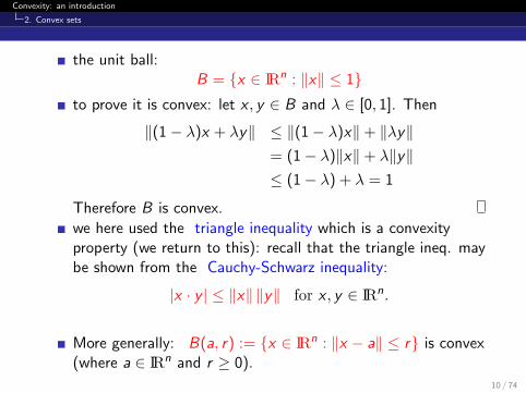
the unit ball:B = {x ∈ IRn : ‖x‖ ≤ 1}
to prove it is convex: let x , y ∈ B and λ ∈ [0, 1]. Then
‖(1− λ)x + λy‖ ≤ ‖(1− λ)x‖+ ‖λy‖= (1− λ)‖x‖+ λ‖y‖≤ (1− λ) + λ = 1
Therefore B is convex.
we here used the triangle inequality which is a convexityproperty (we return to this): recall that the triangle ineq. maybe shown from the Cauchy-Schwarz inequality:
|x · y | ≤ ‖x‖ ‖y‖ for x , y ∈ IRn.
More generally: B(a, r) := {x ∈ IRn : ‖x − a‖ ≤ r} is convex(where a ∈ IRn and r ≥ 0).
10 / 74
Convexity: an introduction
2. Convex sets
Linear systems and polyhedra
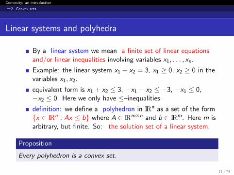
By a linear system we mean a finite set of linear equationsand/or linear inequalities involving variables x1, . . . , xn.
Example: the linear system x1 + x2 = 3, x1 ≥ 0, x2 ≥ 0 in thevariables x1, x2.
equivalent form is x1 + x2 ≤ 3, −x1 − x2 ≤ −3, −x1 ≤ 0,−x2 ≤ 0. Here we only have ≤–inequalities
definition: we define a polyhedron in IRn as a set of the form{x ∈ IRn : Ax ≤ b} where A ∈ IRm×n and b ∈ IRm. Here m isarbitrary, but finite. So: the solution set of a linear system.
Proposition
Every polyhedron is a convex set.
11 / 74
Convexity: an introduction
2. Convex sets
Proposition
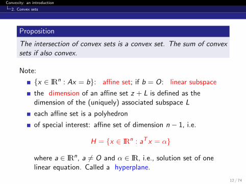
The intersection of convex sets is a convex set. The sum of convexsets if also convex.
Note:
{x ∈ IRn : Ax = b}: affine set; if b = O: linear subspace
the dimension of an affine set z + L is defined as thedimension of the (uniquely) associated subspace L
each affine set is a polyhedron
of special interest: affine set of dimension n − 1, i.e.
H = {x ∈ IRn : aT x = α}
where a ∈ IRn, a 6= O and α ∈ IR, i.e., solution set of onelinear equation. Called a hyperplane.
12 / 74
Convexity: an introduction
2. Convex sets
LP and convexity
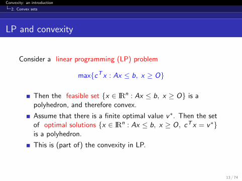
Consider a linear programming (LP) problem
max{cT x : Ax ≤ b, x ≥ O}
Then the feasible set {x ∈ IRn : Ax ≤ b, x ≥ O} is apolyhedron, and therefore convex.
Assume that there is a finite optimal value v∗. Then the setof optimal solutions {x ∈ IRn : Ax ≤ b, x ≥ O, cT x = v∗}is a polyhedron.
This is (part of) the convexity in LP.
13 / 74
Convexity: an introduction
3. Convex hulls
Convex hulls
convex hull
Caratheodory’s theorem
polytopes
linear optimization over polytopes
14 / 74
Convexity: an introduction
3. Convex hulls
Convex hulls
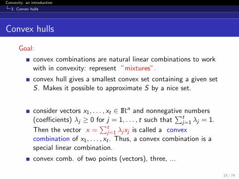
Goal:
convex combinations are natural linear combinations to workwith in convexity: represent ”mixtures”.
convex hull gives a smallest convex set containing a given setS . Makes it possible to approximate S by a nice set.
consider vectors x1, . . . , xt ∈ IRn and nonnegative numbers(coefficients) λj ≥ 0 for j = 1, . . . , t such that
∑tj=1 λj = 1.
Then the vector x =∑t
j=1 λjxj is called a convexcombination of x1, . . . , xt . Thus, a convex combination is aspecial linear combination.
convex comb. of two points (vectors), three, ...
15 / 74
Convexity: an introduction
3. Convex hulls
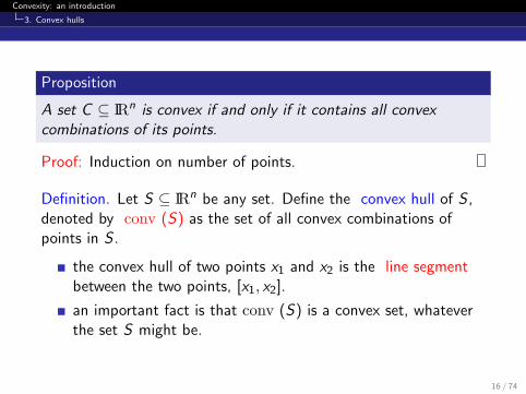
Proposition
A set C ⊆ IRn is convex if and only if it contains all convexcombinations of its points.
Proof: Induction on number of points.
Definition. Let S ⊆ IRn be any set. Define the convex hull of S ,denoted by conv (S) as the set of all convex combinations ofpoints in S .
the convex hull of two points x1 and x2 is the line segmentbetween the two points, [x1, x2].
an important fact is that conv (S) is a convex set, whateverthe set S might be.
16 / 74
Convexity: an introduction
3. Convex hulls
Proposition
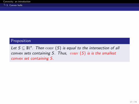
Let S ⊆ IRn. Then conv (S) is equal to the intersection of allconvex sets containing S. Thus, conv (S) is is the smallestconvex set containing S.
17 / 74
Convexity: an introduction
3. Convex hulls
A ”special kind” of convex hull
what happens if we take the convex hull of a finite set ofpoints?
Definition. A set P ⊂ IRn is called a polytope if it is the convexhull of a finite set of points in IRn.
polytopes have been studied a lot during the history ofmathematics
Platonian solids
important in many branches of mathematics, pure and applied.
in optimization: highly relevant in, especially, linearprogramming and discrete optimization.
18 / 74
Convexity: an introduction
3. Convex hulls
Linear optimization over polytopes
Considermax{cT x : x ∈ conv ({x1, . . . , xt}}
where c ∈ IRn.
Each x ∈ P may be written as x =∑t
j=1 λjxj for some λj ≥ 0,
j = 1, . . . , t where∑
j λj = 1. Define v∗ = maxj cT xj . Then
cT x = cT∑
j
λjxj =t∑
j=1
λjcT xj ≤
t∑j=1
λjv∗ = v∗
t∑j=1
λj = v∗.
The set of optimal solutions is
conv ({xj : j ∈ J})where J is the set of indices j satisfying cT xj = v∗.This is a subpolytope of the given polytope (actually aso-called face). Computationally OK if ”few” points. 19 / 74
Convexity: an introduction
3. Convex hulls
Caratheodory’s theorem
The following result says that a convex combination of “many”points may be reduced by using “fewer” points.
Theorem
Let S ⊆ IRn. Then each x ∈ conv (S) may be written as a convexcombination of (say) m affinely independent points in S. Inparticular, m ≤ n + 1.
Try to construct a proof!
20 / 74
Convexity: an introduction
3. Convex hulls
Two consequences
k + 1 vectors x0, x1, . . . , xk ∈ IRn are called affinelyindependent if the k vectors x1 − x0, . . . , xk − x0 are linearlyindependent.
A simplex is the convex hull of a affinely independent points.
Proposition
Every polytope in IRn can be written as the union of a finitenumber of simplices.
Proposition
Every polytope in IRn is compact, i.e., closed and bounded.
21 / 74
Convexity: an introduction
4. Projection and separation
4. Projection and separation
nearest points
separating and supporting hyperplanes
Farkas’ lemma
22 / 74
Convexity: an introduction
4. Projection and separation
Projection
Approximation problem: Given a set S and a point x outside thatset, find a nearest point to x in S !
Question 1: does a nearest point exist?
Question 2: if it does, is it unique?
Question 3: how can we compute a nearest point?
convexity is central here!
23 / 74
Convexity: an introduction
4. Projection and separation
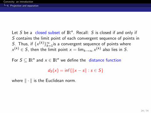
Let S be a closed subset of IRn. Recall: S is closed if and only ifS contains the limit point of each convergent sequence of points inS . Thus, if {x (k)}∞k=1is a convergent sequence of points wherex (k) ∈ S , then the limit point x = limk→∞ x (k) also lies in S .
For S ⊆ IRn and x ∈ IRn we define the distance function
dS(x) = inf{‖x − s‖ : s ∈ S}
where ‖ · ‖ is the Euclidean norm.
24 / 74
Convexity: an introduction
4. Projection and separation
Nearest point
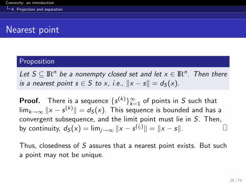
Proposition
Let S ⊆ IRn be a nonempty closed set and let x ∈ IRn. Then thereis a nearest point s ∈ S to x, i.e., ‖x − s‖ = dS(x).
Proof. There is a sequence {s(k)}∞k=1 of points in S such thatlimk→∞ ‖x − s(k)‖ = dS(x). This sequence is bounded and has aconvergent subsequence, and the limit point must lie in S . Then,by continuity, dS(x) = limj→∞ ‖x − s(ij )‖ = ‖x − s‖.
Thus, closedness of S assures that a nearest point exists. But sucha point may not be unique.
25 / 74
Convexity: an introduction
4. Projection and separation
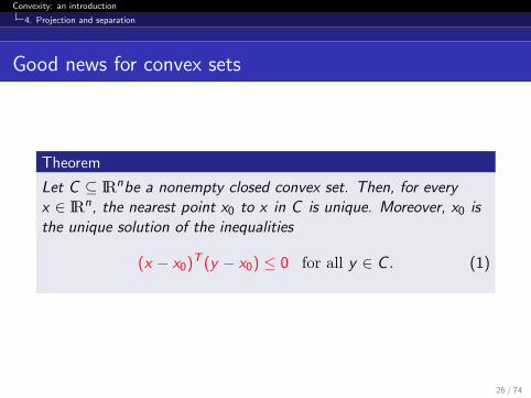
Good news for convex sets
Theorem
Let C ⊆ IRnbe a nonempty closed convex set. Then, for everyx ∈ IRn, the nearest point x0 to x in C is unique. Moreover, x0 isthe unique solution of the inequalities
(x − x0)T (y − x0) ≤ 0 for all y ∈ C . (1)
26 / 74
Convexity: an introduction
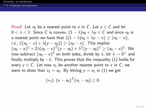
4. Projection and separation
Proof: Let x0 be a nearest point to x in C . Let y ∈ C and let0 < λ < 1. Since C is convex, (1− λ)x0 + λy ∈ C and since x0 isa nearest point we have that ‖(1− λ)x0 + λy − x‖ ≥ ‖x0 − x‖,i.e., ‖(x0 − x) + λ(y − x0)‖ ≥ ‖x0 − x‖. This implies‖x0 − x‖2 + 2λ(x0 − x)T (y − x0) + λ2‖y − x0‖2 ≥ ‖x0 − x‖2. Wenow subtract ‖x0 − x‖2 on both sides, divide by λ, let λ→ 0+ andfinally multiply by −1. This proves that the inequality (1) holds forevery y ∈ C . Let now x1 be another nearest point to x in C ; wewant to show that x1 = x0. By letting y = x1 in (1) we get
(∗1) (x − x0)T (x1 − x0) ≤ 0.
27 / 74
Convexity: an introduction
4. Projection and separation
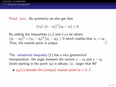
Proof, cont.: By symmetry we also get that
(∗2) (x − x1)T (x0 − x1) ≤ 0.
By adding the inequalities (∗1) and (∗2) we obtain‖x1 − x0‖2 = (x1 − x0)T (x1 − x0) ≤ 0 which implies that x1 = x0.Thus, the nearest point is unique.
The variational inequality (1) has a nice geometricalinterpretation: the angle between the vectors x − x0 and y − x0
(both starting in the point x0) is obtuse, i.e., larger that 90◦.
pC (x) denotes the (unique) nearest point to x in C .
28 / 74
Convexity: an introduction
4. Projection and separation
What’s next?
We shall now discuss supporting hyperplanes and separation ofconvex sets.
Why is this important?
leads to another representation of closed convex sets
may be used to approximate convex functions by simplerfunctions
may be used to prove Farkas’ lemma, and the linearprogramming duality theorem
used in statistics (e.g. decision theory), mathematicalfinance, economics, game theory.
29 / 74
Convexity: an introduction
4. Projection and separation
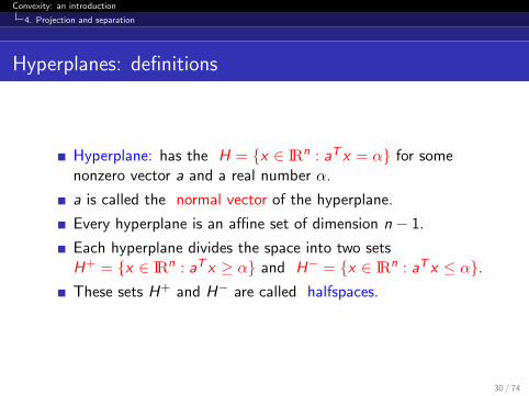
Hyperplanes: definitions
Hyperplane: has the H = {x ∈ IRn : aT x = α} for somenonzero vector a and a real number α.
a is called the normal vector of the hyperplane.
Every hyperplane is an affine set of dimension n − 1.
Each hyperplane divides the space into two setsH+ = {x ∈ IRn : aT x ≥ α} and H− = {x ∈ IRn : aT x ≤ α}.These sets H+ and H− are called halfspaces.
30 / 74
Convexity: an introduction
4. Projection and separation
Definition: Let S ⊂ IRn and let H be a hyperplane in IRn.
If S is contained in one of the halfspaces H+ or H− and H ∩ Sis nonempty, we say that H is a supporting hyperplane of S .
We also say that H supports S at x , for each x ∈ H ∩ S .
31 / 74
Convexity: an introduction
4. Projection and separation
Supporting hyperplanes
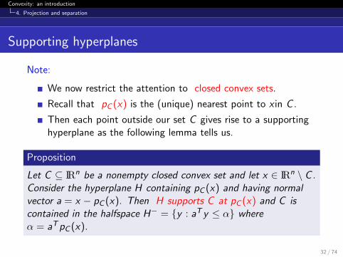
Note:
We now restrict the attention to closed convex sets.
Recall that pC (x) is the (unique) nearest point to x in C .
Then each point outside our set C gives rise to a supportinghyperplane as the following lemma tells us.
Proposition
Let C ⊆ IRn be a nonempty closed convex set and let x ∈ IRn \ C .Consider the hyperplane H containing pC (x) and having normalvector a = x − pC (x). Then H supports C at pC (x) and C iscontained in the halfspace H− = {y : aT y ≤ α} whereα = aT pC (x).
32 / 74
Convexity: an introduction
4. Projection and separation
The proof
Note that a is nonzero as x 6∈ C while pC (x) ∈ C . Then H is thehyperplane with normal vector a and given byaT y = α = aT pC (x). We shall show that C is contained in thehalfspace H−. So, let y ∈ C . Then, by (1) we have(x − pC (x))T (y − pC (x)) ≤ 0, i.e., aT y ≤ aT pC (x) = α asdesired.
33 / 74
Convexity: an introduction
4. Projection and separation
Separation
Define:Ha,α := {x ∈ IRn : aT x = α};H−a,α := {x ∈ IRn : aT x ≤ α};H+
a,α := {x ∈ IRn : aT x ≥ α}.
We say that the hyperplane Ha,α separates two sets S and T ifS ⊆ H−a,α and T ⊆ H+
a,α or vice versa.
Note that both S and T may intersect the hyperplane Ha,α in thisdefinition.
We say that the hyperplane Ha,α strongly separates S and T ifthere is an ε > 0 such that S ⊆ H−a,α−εand T ⊆ H+
a,α+ε or viceversa. This means that
aT x ≤ α− ε for all x ∈ S ;aT x ≥ α + ε for all x ∈ T .
34 / 74
Convexity: an introduction
4. Projection and separation
Strong separation
Theorem
Let C ⊆ IRn be a nonempty closed convex set and assume thatx ∈ IRn \ C . Then C and x can be strongly separated.
Proof. Let H be the hyperplane containing pC (x) and havingnormal vector x − pC (x). From the previous proposition we knowthat H supports C at pC (x). Moreover x 6= pC (x) (as x 6∈ C ).Consider the hyperplane H∗ which is parallel to H (i.e., having thesame normal vector) and contains the point (1/2)(x + pC (x)).Then H∗ strongly separates x and C .
35 / 74
Convexity: an introduction
4. Projection and separation
An important consequence
Exterior description of closed convex sets:
Corollary
Let C ⊆ IRn be a nonempty closed convex set. Then C is theintersection of all its supporting halfspaces.
36 / 74
Convexity: an introduction
4. Projection and separation
Another application: Farkas’ lemma
Theorem
Let A ∈ IRm×n and b ∈ IRm. Then there exists an x ≥ Osatisfying Ax = b if and only if for each y ∈ IRm with yT A ≥ O italso holds that yT b ≥ 0.
Proof: Consider the closed convex cone (define!!)C = cone ({a1, . . . , an}) ⊆ IRm. Observe: Ax = b has anonnegative solution simply means simply (geometrically) thatb ∈ C .Assume now that Ax = b and x ≥ O. If yT a ≥ O, thenyT b = yT (ax) = (yT a)x ≥ 0.
37 / 74
Convexity: an introduction
4. Projection and separation
Proof, cont.: Conversely, if Ax = b has no nonnegative solution,then b 6∈ C . But then, by Strong Separation Theorem, C and bcan be strongly separated, so there is a nonzero vector y ∈ IRn andα ∈ IRwith yT x ≥ α for each x ∈ C and yT b < α. As O ∈ C , wehave α ≤ 0. Moreover yT aj ≥ 0 so yT a ≥ O. Since yT b < 0 wehave proved the other direction of Farkas’ lemma.
38 / 74
Convexity: an introduction
5. Representation of convex sets
5. Representation of convex sets
study (very briefly) the structure of convex sets
involves the notions: faces, extreme points and extremehalflines
an important subfield: the theory (and application) ofpolyhedra and polytopes
39 / 74
Convexity: an introduction
5. Representation of convex sets
Faces
Definition. Let C be a convex set in IRn. A convex subset F of Cis a face of C whenever the following condition holds:
if x1, x2 ∈ C is such that (1− λ)x1 + λx2 ∈ F for some0 < λ < 1, then x1, x2 ∈ F .
So: if a relative interior point of the line segment between twopoints of C lies in F , then the whole line segment between thesetwo points lies in F .
Note: the empty set and C itself are (trivial) faces of C .
Example:
faces of the unit square and unit circle
40 / 74
Convexity: an introduction
5. Representation of convex sets
Exposed faces
Definition. Let C ⊆ IRn be a convex set and H a supportinghyperplane of C . Then the intersection C ∩H is called an exposedface of C .
Relation between faces and exposed faces:
Let C be a nonempty convex set in IRn. Then each exposedface of C is also a face of C .
For polyhedra: exposed faces and faces are the same!
41 / 74
Convexity: an introduction
5. Representation of convex sets
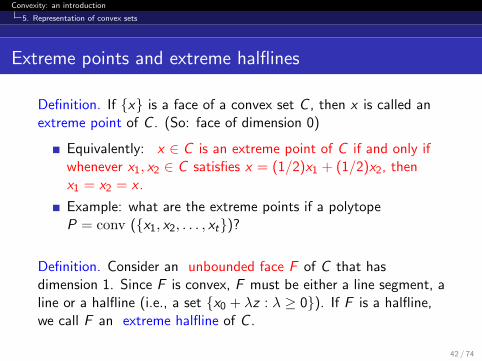
Extreme points and extreme halflines
Definition. If {x} is a face of a convex set C , then x is called anextreme point of C . (So: face of dimension 0)
Equivalently: x ∈ C is an extreme point of C if and only ifwhenever x1, x2 ∈ C satisfies x = (1/2)x1 + (1/2)x2, thenx1 = x2 = x .
Example: what are the extreme points if a polytopeP = conv ({x1, x2, . . . , xt})?
Definition. Consider an unbounded face F of C that hasdimension 1. Since F is convex, F must be either a line segment, aline or a halfline (i.e., a set {x0 + λz : λ ≥ 0}). If F is a halfline,we call F an extreme halfline of C .
42 / 74
Convexity: an introduction
5. Representation of convex sets
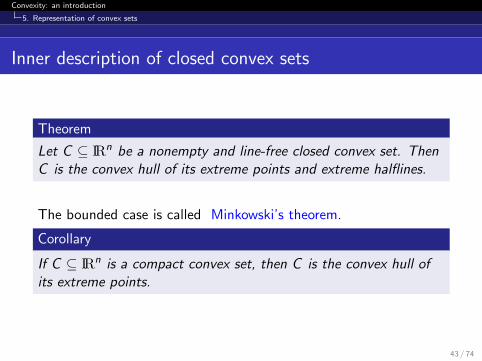
Inner description of closed convex sets
Theorem
Let C ⊆ IRn be a nonempty and line-free closed convex set. ThenC is the convex hull of its extreme points and extreme halflines.
The bounded case is called Minkowski’s theorem.
Corollary
If C ⊆ IRn is a compact convex set, then C is the convex hull ofits extreme points.
43 / 74
Convexity: an introduction
5. Representation of convex sets
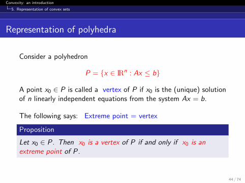
Representation of polyhedra
Consider a polyhedron
P = {x ∈ IRn : Ax ≤ b}
A point x0 ∈ P is called a vertex of P if x0 is the (unique) solutionof n linearly independent equations from the system Ax = b.
The following says: Extreme point = vertex
Proposition
Let x0 ∈ P. Then x0 is a vertex of P if and only if x0 is anextreme point of P.
44 / 74
Convexity: an introduction
5. Representation of convex sets
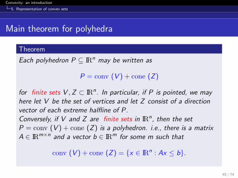
Main theorem for polyhedra
Theorem
Each polyhedron P ⊆ IRn may be written as
P = conv (V ) + cone (Z )
for finite sets V ,Z ⊂ IRn. In particular, if P is pointed, we mayhere let V be the set of vertices and let Z consist of a directionvector of each extreme halfline of P.Conversely, if V and Z are finite sets in IRn, then the setP = conv (V ) + cone (Z ) is a polyhedron. i.e., there is a matrixA ∈ IRm×n and a vector b ∈ IRm for some m such that
conv (V ) + cone (Z ) = {x ∈ IRn : Ax ≤ b}.
45 / 74
Convexity: an introduction
6. Convex functions
6. Convex functions
convex functions of a single variable
... of several variables
characterizations
properties, and optimization
46 / 74
Convexity: an introduction
6. Convex functions
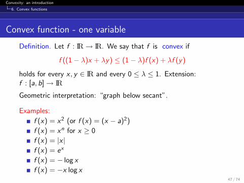
Convex function - one variable
Definition. Let f : IR→ IR. We say that f is convex if
f ((1− λ)x + λy) ≤ (1− λ)f (x) + λf (y)
holds for every x , y ∈ IR and every 0 ≤ λ ≤ 1. Extension:f : [a, b]→ IR
Geometric interpretation: “graph below secant”.
Examples:
f (x) = x2 (or f (x) = (x − a)2)
f (x) = xn for x ≥ 0
f (x) = |x |f (x) = ex
f (x) = − log x
f (x) = −x log x47 / 74
Convexity: an introduction
6. Convex functions
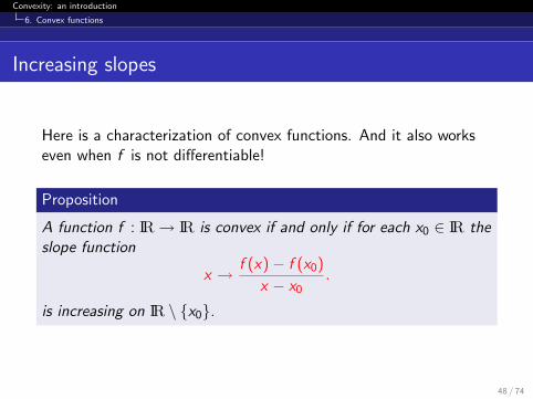
Increasing slopes
Here is a characterization of convex functions. And it also workseven when f is not differentiable!
Proposition
A function f : IR→ IR is convex if and only if for each x0 ∈ IR theslope function
x → f (x)− f (x0)
x − x0.
is increasing on IR \ {x0}.
48 / 74
Convexity: an introduction
6. Convex functions
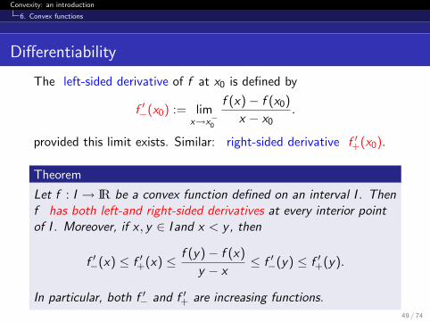
Differentiability
The left-sided derivative of f at x0 is defined by
f ′−(x0) := limx→x−0
f (x)− f (x0)
x − x0.
provided this limit exists. Similar: right-sided derivative f ′+(x0).
Theorem
Let f : I → IR be a convex function defined on an interval I . Thenf has both left-and right-sided derivatives at every interior pointof I . Moreover, if x , y ∈ I and x < y, then
f ′−(x) ≤ f ′+(x) ≤ f (y)− f (x)
y − x≤ f ′−(y) ≤ f ′+(y).
In particular, both f ′− and f ′+ are increasing functions.
49 / 74
Convexity: an introduction
6. Convex functions
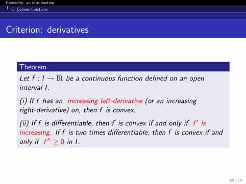
Criterion: derivatives
Theorem
Let f : I → IR be a continuous function defined on an openinterval I .
(i) If f has an increasing left-derivative (or an increasingright-derivative) on, then f is convex.
(ii) If f is differentiable, then f is convex if and only if f ′ isincreasing. If f is two times differentiable, then f is convex if andonly if f ′′ ≥ 0 in I .
50 / 74
Convexity: an introduction
6. Convex functions
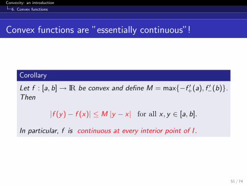
Convex functions are ”essentially continuous”!
Corollary
Let f : [a, b]→ IR be convex and define M = max{−f ′+(a), f ′−(b)}.Then
|f (y)− f (x)| ≤ M |y − x | for all x , y ∈ [a, b].
In particular, f is continuous at every interior point of I .
51 / 74
Convexity: an introduction
6. Convex functions
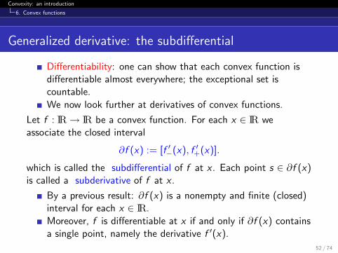
Generalized derivative: the subdifferential
Differentiability: one can show that each convex function isdifferentiable almost everywhere; the exceptional set iscountable.We now look further at derivatives of convex functions.
Let f : IR→ IR be a convex function. For each x ∈ IR weassociate the closed interval
∂f (x) := [f ′−(x), f ′+(x)].
which is called the subdifferential of f at x . Each point s ∈ ∂f (x)is called a subderivative of f at x .
By a previous result: ∂f (x) is a nonempty and finite (closed)interval for each x ∈ IR.Moreover, f is differentiable at x if and only if ∂f (x) containsa single point, namely the derivative f ′(x).
52 / 74
Convexity: an introduction
6. Convex functions
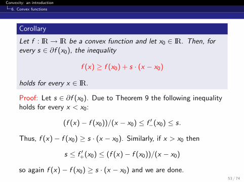
Corollary
Let f : IR→ IR be a convex function and let x0 ∈ IR. Then, forevery s ∈ ∂f (x0), the inequality
f (x) ≥ f (x0) + s · (x − x0)
holds for every x ∈ IR.
Proof: Let s ∈ ∂f (x0). Due to Theorem 9 the following inequalityholds for every x < x0:
(f (x)− f (x0))/(x − x0) ≤ f ′−(x0) ≤ s.
Thus, f (x)− f (x0) ≥ s · (x − x0). Similarly, if x > x0 then
s ≤ f ′+(x0) ≤ (f (x)− f (x0))/(x − x0)
so again f (x)− f (x0) ≥ s · (x − x0) and we are done.53 / 74
Convexity: an introduction
6. Convex functions
Support
Consider again the inequality:
f (x) ≥ f (x0) + s · (x − x0) = L(x)
L can be seen as a linear approximation to f at x0. We saythat L supports f at x0; this means that L(x0) = f (x0) andL(x) ≤ f (x) for every x .
So L underestmates f everywhere!
54 / 74
Convexity: an introduction
6. Convex functions
Global minimum
We call x0 a global minimum if
f (x0) ≤ f (x) for all x ∈ IR.
Weaker notion: local minimum: smallest function value in someneighborhood of x0.
In general it is hard to find a global minimum of a function.
But when f is convex this is much easier!
55 / 74
Convexity: an introduction
6. Convex functions
The following result may be derived from
f (x) ≥ f (x0) + s · (x − x0) = f (x0).
Corollary
Let f : IR→ IR be a convex function. Then the following threestatements are equivalent.
(i) x0 is a local minimum for f .
(ii) x0 is a global minimum for f .
(iii) 0 ∈ ∂f (x0).
56 / 74
Convexity: an introduction
6. Convex functions
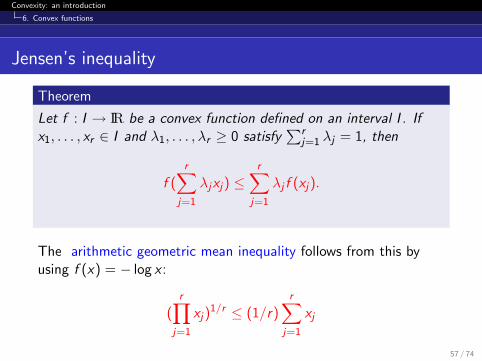
Jensen’s inequality
Theorem
Let f : I → IR be a convex function defined on an interval I . Ifx1, . . . , xr ∈ I and λ1, . . . , λr ≥ 0 satisfy
∑rj=1 λj = 1, then
f (r∑
j=1
λjxj) ≤r∑
j=1
λj f (xj).
The arithmetic geometric mean inequality follows from this byusing f (x) = − log x :
(r∏
j=1
xj)1/r ≤ (1/r)
r∑j=1
xj
57 / 74
Convexity: an introduction
6. Convex functions
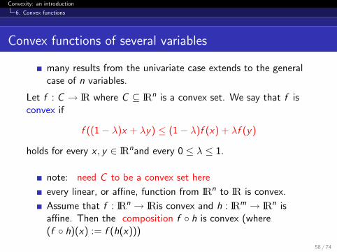
Convex functions of several variables
many results from the univariate case extends to the generalcase of n variables.
Let f : C → IR where C ⊆ IRn is a convex set. We say that f isconvex if
f ((1− λ)x + λy) ≤ (1− λ)f (x) + λf (y)
holds for every x , y ∈ IRnand every 0 ≤ λ ≤ 1.
note: need C to be a convex set here
every linear, or affine, function from IRn to IR is convex.
Assume that f : IRn → IRis convex and h : IRm → IRn isaffine. Then the composition f ◦ h is convex (where(f ◦ h)(x) := f (h(x)))
58 / 74
Convexity: an introduction
6. Convex functions
Jensen’s inequality, more generally
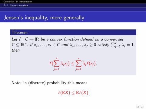
Theorem
Let f : C → IR be a convex function defined on a convex setC ⊆ IRn. If x1, . . . , xr ∈ C and λ1, . . . , λr ≥ 0 satisfy
∑rj=1 λj = 1,
then
f (r∑
j=1
λjxj) ≤r∑
j=1
λj f (xj).
Note: in (discrete) probability this means
f (EX ) ≤ Ef (X )
59 / 74
Convexity: an introduction
6. Convex functions
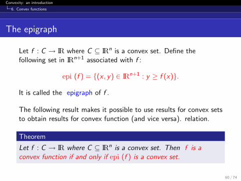
The epigraph
Let f : C → IR where C ⊆ IRn is a convex set. Define thefollowing set in IRn+1 associated with f :
epi (f ) = {(x , y) ∈ IRn+1 : y ≥ f (x)}.
It is called the epigraph of f .
The following result makes it possible to use results for convex setsto obtain results for convex function (and vice versa). relation.
Theorem
Let f : C → IR where C ⊆ IRn is a convex set. Then f is aconvex function if and only if epi (f ) is a convex set.
60 / 74
Convexity: an introduction
6. Convex functions
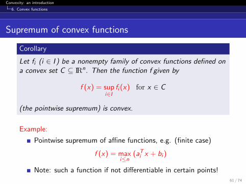
Supremum of convex functions
Corollary
Let fi (i ∈ I ) be a nonempty family of convex functions defined ona convex set C ⊆ IRn. Then the function f given by
f (x) = supi∈I
fi (x) for x ∈ C
(the pointwise supremum) is convex.
Example:
Pointwise supremum of affine functions, e.g. (finite case)
f (x) = maxi≤n
(aTi x + bi )
Note: such a function if not differentiable in certain points!61 / 74
Convexity: an introduction
6. Convex functions
The support function
Let P be a polytope in IRn, say P = conv ({v1, . . . , vt}). Define
ψP(c) := max{cT x : x ∈ P}.which is the optimal value of this LP problem. This function ψP iscalled the support function of P.
ψP is a convex function! Because it is the pointwisesupremum of the linear functions c → cT vj (j ≤ t). Thismaximum is attained in a vertex (since the objective functionis linear).More generally: the support function ψC of a compactconvex set C is convex. Similar proof, but we take thesupremum of an infinite family of linear functions; one foreach extreme point of C .Here we used Minkowski’s theorem saying that a compactconvex set is the convex hull of its extreme points.
62 / 74
Convexity: an introduction
6. Convex functions
Directional derivative
Let f : IRn → IR be a function and let x0 ∈ IRn and z ∈ IRn,z 6= O. The directional derivative of f at x0 is
f ′(x0; z) = limt→0
f (x0 + tz)− f (x0)
t
provided the limit exists. Special case: f ′(x0; ej) = ∂f (x)∂xj
.
Let f : IRn → IR be a convex function and consider a lineL = {x0 + λz : λ ∈ IR} where x0 is a point on the line and z is thedirection vector of L. Define the function g : IR→ IR by
g(t) = f (x0 + tz) for t ∈ IR.
One can prove that g is a convex function (of a single variable).
63 / 74
Convexity: an introduction
6. Convex functions
Thus, the restriction g of a convex function f to any line isanother convex function.
A consequence of this result is that a convex functionf : IRn → IR has one-sided directional derivatives:
g ′+(0) = limt→0+(g(t)− g(0))/t
= limt→0+(f (x0 + tz)− f (x0))/t
= f ′+(x0; z)
64 / 74
Convexity: an introduction
6. Convex functions
Continuity
Theorem
Let f : C → IR be a convex function defined on an open convexset C ⊆ IRn. Then f is continuous on C .
65 / 74
Convexity: an introduction
6. Convex functions
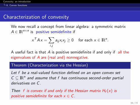
Characterization of convexity
We now recall a concept from linear algebra: a symmetric matrixA ∈ IRn×n is positive semidefinite if
xT A x =∑i ,j
aijxixj ≥ 0 for each x ∈ IRn.
A useful fact is that A is positive semidefinite if and only if all theeigenvalues of A are (real and) nonnegative.
Theorem (Characterization via the Hessian)
Let f be a real-valued function defined on an open convex setC ⊆ IRn and assume that f has continuous second-order partialderivatives on C .
Then f is convex if and only if the Hessian matrix Hf (x) ispositive semidefinite for each x ∈ C .
66 / 74
Convexity: an introduction
6. Convex functions
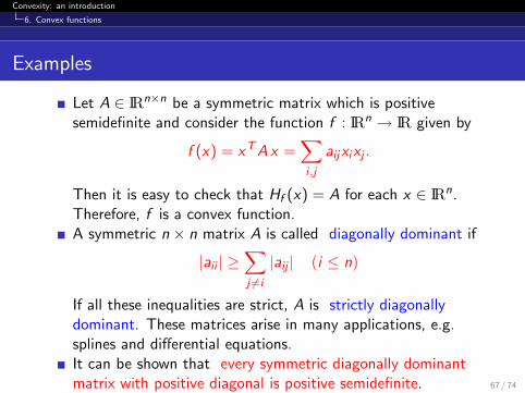
Examples
Let A ∈ IRn×n be a symmetric matrix which is positivesemidefinite and consider the function f : IRn → IR given by
f (x) = xT A x =∑i ,j
aijxixj .
Then it is easy to check that Hf (x) = A for each x ∈ IRn.Therefore, f is a convex function.A symmetric n × n matrix A is called diagonally dominant if
|aii | ≥∑j 6=i
|aij | (i ≤ n)
If all these inequalities are strict, A is strictly diagonallydominant. These matrices arise in many applications, e.g.splines and differential equations.It can be shown that every symmetric diagonally dominantmatrix with positive diagonal is positive semidefinite. 67 / 74
Convexity: an introduction
6. Convex functions
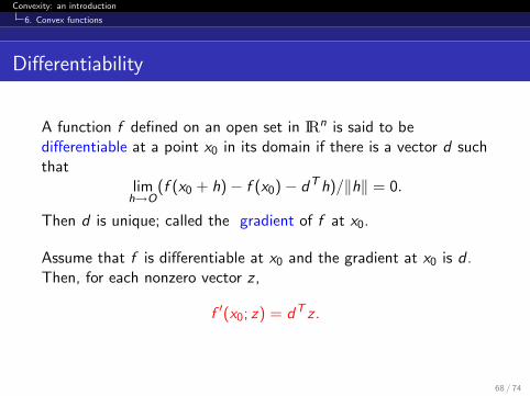
Differentiability
A function f defined on an open set in IRn is said to bedifferentiable at a point x0 in its domain if there is a vector d suchthat
limh→O
(f (x0 + h)− f (x0)− dT h)/‖h‖ = 0.
Then d is unique; called the gradient of f at x0.
Assume that f is differentiable at x0 and the gradient at x0 is d .Then, for each nonzero vector z ,
f ′(x0; z) = dT z .
68 / 74
Convexity: an introduction
6. Convex functions
Partial derivatives, gradients
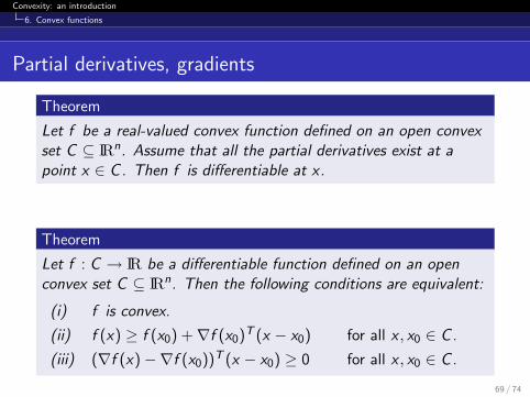
Theorem
Let f be a real-valued convex function defined on an open convexset C ⊆ IRn. Assume that all the partial derivatives exist at apoint x ∈ C . Then f is differentiable at x.
Theorem
Let f : C → IR be a differentiable function defined on an openconvex set C ⊆ IRn. Then the following conditions are equivalent:
(i) f is convex.
(ii) f (x) ≥ f (x0) +∇f (x0)T (x − x0) for all x , x0 ∈ C .
(iii) (∇f (x)−∇f (x0))T (x − x0) ≥ 0 for all x , x0 ∈ C .
69 / 74
Convexity: an introduction
6. Convex functions
Consider a convex function f and an affine function h, bothdefined on a convex set C ⊆ IRn.We say that h : IRn → IR supports f at x0 if h(x) ≤ f (x) for everyx and h(x0) = f (x0).
Theorem
Let f : C → IR be a convex function defined on a convex setC ⊆ IRn. Then f has a supporting (affine) function at every point.Moreover, f is the pointwise supremum of all its (affine)supporting functions.
70 / 74
Convexity: an introduction
6. Convex functions
Global minimum
Corollary
Let f : C → IR be a differentiable convex function defined on anopen convex set C ⊆ IRn. Let x∗ ∈ C . Then the following threestatements are equivalent.
(i) x∗ is a local minimum for f .
(ii) x∗ is a global minimum for f .
(iii) ∇f (x∗) = O (i.e., all partial derivatives at x∗ are zero).
71 / 74
Convexity: an introduction
6. Convex functions
Subgradients
Definition. Let f be a convex function and x0 ∈ IRn. Then s ∈ IRn
is called a subgradient of f at x0 if
f (x) ≥ f (x0) + sT (x − x0) for all x ∈ IRn
The set of all subgradients of f at x0 is called thesubdifferential of f at x0, and it is denoted by ∂f (x0).
Here is the basic result on the subdifferential.
Theorem
Let f : IRn → IR be a convex function, and x0 ∈ IRn. Then ∂f (x0)is a nonempty, compact and convex set in IRn.
72 / 74
Convexity: an introduction
6. Convex functions
Global minimum, again
Moreover, we have the following theorem on minimum of convexfunctions.
Corollary
Let f : C → IR be a convex function defined on an open convexset C ⊆ IRn. Let x∗ ∈ C . Then the following three statements areequivalent.
(i) x∗ is a local minimum for f .
(ii) x∗ is a global minimum for f .
(iii) O ∈ ∂f (x∗) (O is a subgradient).
73 / 74
Convexity: an introduction
6. Convex functions
Final comments ...
This means that convex problems are attractive, andsometimes other problems are reformulated/modfied intoconvex problems
Algorithms exist for minimizing convex functions, with orwiothout constraints.
So gradient-like methods for differentiable functions areextended into subgradient methods for general convexfunctions.
More complicated, but efficient methods exist.
74 / 74