Noname manuscript No.(will be inserted by the editor)

Coordinate Descent Algorithm for Covariance Graphical Lasso

Hao Wang

Received: date / Accepted: date

Abstract Bien and Tibshirani (2011) have proposed a

covariance graphical lasso method that applies a lasso

penalty on the elements of the covariance matrix. This

method is definitely useful because it not only produces

sparse and positive definite estimates of the covariance

matrix but also discovers marginal independence struc-

tures by generating exact zeros in the estimated co-

variance matrix. However, the objective function is not

convex, making the optimization challenging. Bien and

Tibshirani (2011) described a majorize-minimize ap-

proach to optimize it. We develop a new optimization

method based on coordinate descent. We discuss the

convergence property of the algorithm. Through sim-

ulation experiments, we show that the new algorithm

has a number of advantages over the majorize-minimize

approach, including its simplicity, computing speed andnumerical stability. Finally, we show that the cyclic ver-

sion of the coordinate descent algorithm is more effi-

cient than the greedy version.

Keywords Coordinate descent · Covariance graphical

lasso · Covariance matrix estimation · L1 penalty · MM

algorithm · Marginal independence · Regularization ·Shrinkage · Sparsity

1 Introduction

Bien and Tibshirani (2011) proposed a covariance graph-

ical lasso procedure for simultaneously estimating co-

variance matrix and marginal dependence structures.

Hao WangDepartment of Statistics, University of South Carolina,Columbia, South Carolina 29208, U.S.A.E-mail: haowang@sc.edu

1 Let S be the sample covariance matrix such that

S = Y′Y/n where Y(n × p) is the data matrix of p

variables and n samples. A basic version of their co-

variance graphical lasso problem is to minimize the fol-

lowing objective function:

g(Σ) = log(detΣ) + tr(SΣ−1) + ρ||Σ||1, (1)

over the space of positive definite matrices M+ with

ρ ≥ 0 being the shrinkage parameter. Here, Σ = (σij) is

the p× p covariance matrix and ||Σ||1 =∑

1≤i,j≤p |σij |is the L1-norm of Σ. A general version of the covariance

graphical lasso in Bien and Tibshirani (2011) allows

different shrinkage parameters for different elements in

Σ. To ease exposition, we describe our methods in the

context of one common shrinkage parameter as in (1).

All of our results can be extended to the general version

of different shrinkage parameters with little difficulty.

Because of the L1-norm term, the covariance graph-

ical lasso is able to set some of the off-diagonal elements

of Σ exactly equal to zero in its minimum point of (1).

Zeros in Σ encode marginal independence structures

among the components of a multivariate normal ran-

dom vector with covariance matrix Σ. It is distinctly

different from the concentration graphical models (also

referred to as covariance selection models due to Demp-

ster 1972) where zeros are in the concentration matrix

Σ−1 and are associated with conditional independence.

The objective function (1) is not convex, impos-

ing computational challenges for minimizing it. Bien

and Tibshirani (2011) proposed a majorize-minimize

approach to approximately minimize (1). In this paper,

we develop the coordinate descent algorithm for min-

imizing (1). We discuss the convergence property and

1 An unpublished PhD dissertation Lin (2010) may con-sider the covariance graphical lasso method earlier than Bienand Tibshirani (2011).

2 Hao Wang

investigate its computational efficiency through simu-

lation studies. In comparison with Bien and Tibshirani

(2011)’s algorithm, the coordinate descent algorithm is

vastly simpler to implement, substantially faster to run

and numerically more stable in our tests.

Coordinate descent is not new to the model fitting

for regularized problems. It is shown to be very com-

petitive for solving convex and some non-convex pe-

nalized regression models (Fu, 1998; Sardy et al, 2000;

Friedman et al, 2007; Wu and Lange, 2008; Breheny

and Huang, 2011) as well as the concentration graphi-

cal models (Friedman et al, 2008). However, the devel-

opment of this general algorithm to covariance graphi-

cal lasso models is new and unexplored before. In this

sense, our work also contributes to the literature by doc-

umenting the usefulness of this important algorithm for

the class of covariance graphical lasso models.

Finally, we investigate if the proposed coordinate

descent can be further improved by comparing it with

two additional competitors: a greedy coordinate descent

algorithm and a new majorize-minimize algorithm. We

show that the cyclic coordinate descent algorithm re-

mains to be superior to these competitors in efficiency.

2 Coordinate descent algorithm

2.1 Algorithm description

To minimize (1) based on the simple idea of coordinate

descent, we show how to update Σ one column and

row at a time while holding all of the rest elements in

Σ fixed. Without loss of generality, we focus on the last

column and row. Partition Σ and S as follows:

Σ =

(Σ11,σ12

σ′12, σ22

), S =

(S11, s12s′12, s22

), (2)

where (a) Σ11 and S11 are the covariance matrix and

the sample covariance matrix of the first p−1 variables,

respectively; (b) σ12 and s12 are the covariances and

the sample covariances between the first p−1 variables

and the last variable, respectively; and (c) σ22 and s22are the variance and the sample variance of the last

variable, respectively.

Let

β = σ12, γ = σ22 − σ′12Σ−111 σ12,

and apply the block matrix inversion to Σ using blocks

(Σ11,β, γ):

Σ−1 =

(Σ−111 + Σ−111 ββ

′Σ−111 γ−1, −Σ−111 βγ

−1

−β′Σ−111 γ−1, γ−1

). (3)

The three terms in (1) can be expressed as a function

of (β, γ):

log(detΣ) = log(γ) + c1,

tr(SΣ−1) = β′Σ−111 S11Σ−111 βγ

−1 − 2s′12Σ−111 βγ

−1

+s22γ−1 + c2,

ρ||Σ||1 = 2ρ||β||1 + ρ(β′Σ−111 β + γ) + c3,

where c1,c2 and c3 are constants not involving (β, γ).

Dropping off c1,c2 and c3 from (1), we have the follow-

ing objective function with respect to (β, γ):

minβ,γ

{log(γ) + β′Σ−111 S11Σ

−111 βγ

−1 − 2s′12Σ−111 βγ

−1

+ s22γ−1 + 2ρ||β||1 + ρβ′Σ−111 β + ργ

}. (4)

For γ, removing terms in (4) that do not depend on

γ gives

minγ

{log(γ) + aγ−1 + ργ

},

where a = β′Σ−111 S11Σ−111 β− 2s12Σ

−111 β + s22. Clearly,

it is solved by:

γ̂ =

{a if ρ = 0,

(−1 +√

1 + 4aρ)/(2ρ) if ρ 6= 0.(5)

For β, removing terms in (4) that do not depend on

β gives

minβ

{β′Vβ − 2u′β + 2ρ||β||1

}, (6)

where V = (vij) = Σ−111 S11Σ−111 γ

−1 + ρΣ−111 , u =

Σ−111 s12γ−1. The problem in (6) is a lasso problem and

can be efficiently solved by coordinate descent algo-

rithms (Friedman et al, 2007; Wu and Lange, 2008).

Specifically, for j ∈ {1, . . . , p − 1}, the minimum point

of (6) along the coordinate direction in which βj varies

is:

β̂j = S(uj −∑k 6=j

vkj β̂k, ρ)/vjj , (7)

where S is the soft-threshold operator:

S(x, t) = sign(x)(|x| − t)+.

The update (7) is iterated for j = 1, . . . , p− 1, 1, 2, . . . ,

until convergence. We then update the column as (σ12 =

β, σ22 = γ + β′Σ−111 β) followed by cycling through all

columns until convergence. This algorithm can been

viewed as a block coordinate descent method with p

blocks of β’s and another p blocks of γ’s. The algo-

rithm is summarized as follows:

Coordinate descent algorithm Given input (S, ρ),

start with Σ(0), and at the (k + 1)th iteration (k =

0, 1, . . .)

Coordinate Descent Algorithm for Covariance Graphical Lasso 3

1. Let Σ(k+1) = Σ(k).

2. For i = 1, . . . , p,

(a) Partition Σ(k+1) and S as in (2).

(b) Compute γ as in (5).

(c) Solve the lasso problem (6) by repeating (7) until

convergence.

(d) Update σ(k+1)12 = β,σ

(k+1)21 = β′, σ

(k+1)22 = γ +

β′Σ−111 β.

3. Let k = k + 1 and repeat (1)–(3) until convergence.

2.2 Algorithm convergence

The convergence of the proposed block coordinate de-

scent algorithm to a stationary point can be addressed

by the theoretical results for block coordinate descent

methods for non-differentiable minimization by Tseng

(2001). The key to applying the general theory there to

our algorithm is the separability of the non-differentiable

penalty terms in (1). First, from (5) and (6), the ob-

jective function g has a unique minimum point in each

coordinate block. This satisfies the conditions of Part

(c) of Theorem 4.1 in Tseng (2001) and hence implies

that the algorithm converges to a coordinatewise mini-

mum point. Second, because all directional derivatives

exist, by Lemma 3.1 of Tseng (2001), each coordinate-

wise minimum point is a stationary point. A similar ar-

gument has been given by Breheny and Huang (2011)

to show the convergence of coordinate decent algorithm

to a stationary point for nonconvex penalized regression

models.

3 Comparison of algorithms

We conduct a simulation experiment to compare the

performance of the proposed coordinate descent algo-

rithm with Bien and Tibshirani (2011)’s algorithm. We

consider two configurations of Σ:

– A sparse model taken from Bien and Tibshirani

(2011) with σi,i+1 = σi,i−1 = 0.4, σii = δ and zero

otherwise. Here, δ is chosen such that the condition

number of Σ is p.

– A dense model with σii = 2 and σij = 1 for i 6= j.

The algorithm of Bien and Tibshirani (2011) is coded

in R with its built-in functions. To be comparable to it,

we implement the coordinate descent algorithm in R

without writing any functions in a compiled language.

All computations are performed on a Intel Xeon X5680

3.33GHz processor.

For either the sparse model or the dense model,

we consider problem sizes of (p, n) = (100, 200) and

(p, n) = (200, 400), thus a total of four scenarios of

model and size combinations. For each scenario, we

generate 20 datasets and apply the two algorithms to

each of them under a range of ρ values. All computa-

tions are initialized at the sample covariance matrix,

i.e., Σ(0) = S. For Bien and Tibshirani (2011)’s algo-

rithm, we follow the default setting of tuning param-

eters provided by the “spcov” package (http://cran.

r-project.org/web/packages/spcov/index.html). For

the coordinate descent algorithm, we use the same cri-

terion as Bien and Tibshirani (2011)’s algorithm to stop

the iterations: The procedure stops when the change of

the objective function is less than 10−3.

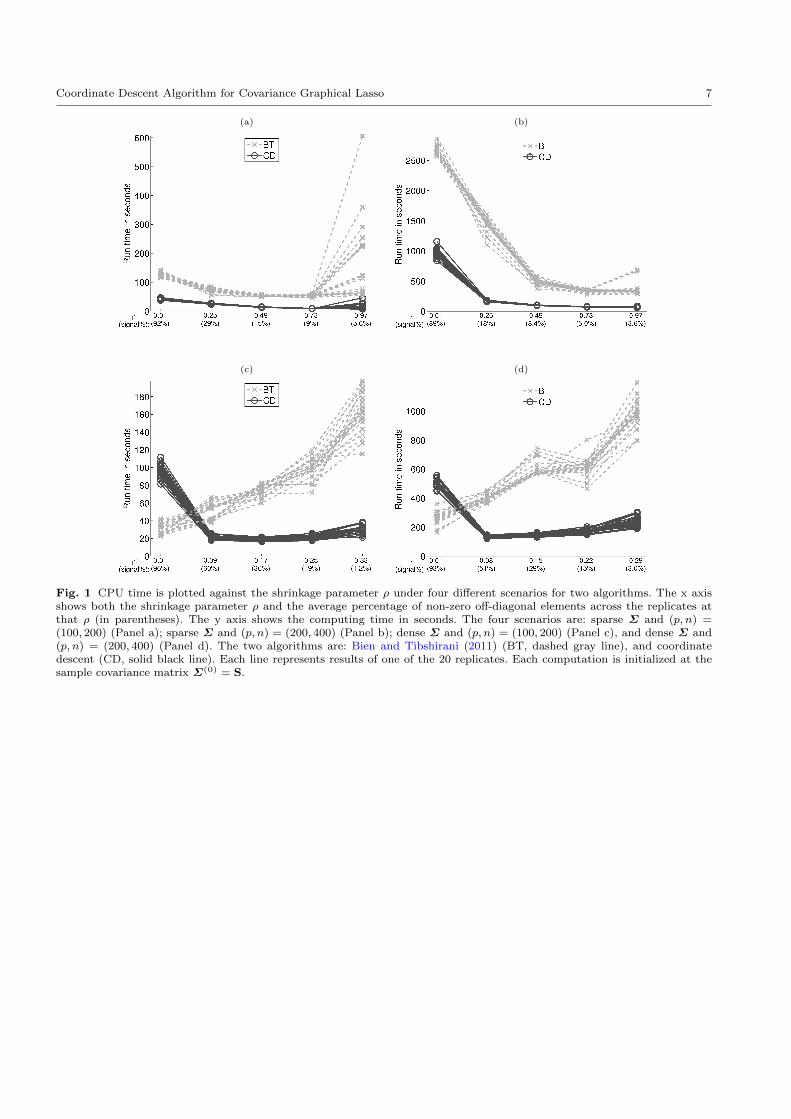
First, we compare the computing speed. The four

panels in Figure 1 display the CPU time under the four

scenarios, respectively. In each panel, CPU time in sec-

onds of the two algorithms for each of the 20 datasets

is plotted against the shrinkage parameter ρ which is

set at five different values that result in a wide range of

sparsity levels in the estimated Σ. As can be seen, the

coordinate descent algorithm is in general substantially

faster than Bien and Tibshirani (2011)’s algorithm ex-

cept when a tiny shrinkage parameter is applied to the

dense model, i.e., ρ = 0.01 in Panel (c) and (d). More-

over, the coordinate descent algorithm seems to be par-

ticularly attractive for sparser models as its run time

generally decreases when the sparsity level increases.

In contrast, the computing time of Bien and Tibshirani

(2011)’s algorithm significantly increases as the spar-

sity level increases under the two dense scenarios. Fi-

nally, the computing time of the coordinate descent al-

gorithm appears to have less variability across multiple

replications than that of Bien and Tibshirani (2011)’s

algorithm, particularly when the estimated Σ is sparse.

This suggests that the coordinate descent algorithm has

more consistent computing time performance.

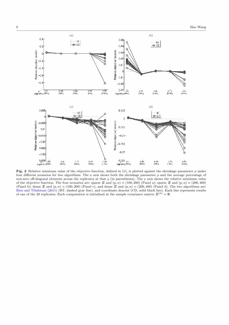
Next, we examine the ability of the algorithms to

find minimum points. To do so, we compute the mini-

mum values of the objective functions achieved by each

algorithm. For each dataset and each ρ, We calculate

the relative minimum values of the objective function

defined as:

g(Σ̂CD)− g(Σ̂BT ), (8)

where Σ̂BT and Σ̂CD are the minimum points found

by Bien and Tibshirani (2011)’s algorithm and the co-

ordinate descent algorithm, respectively. Thus, a nega-

tive value of (8) indicates that the coordinate descent

algorithm finds better points than Bien and Tibshi-

rani (2011)’s algorithm, and a smaller relative minimum

value indicates a better performance of the coordinate

descent algorithm. The four panels in Figure 2 display

the relative minimum values of (8) as functions of the

4 Hao Wang

shrinkage parameter ρ for the four scenarios, respec-

tively. As can be seen, the coordinate descent algorithm

tends to outperforms Bien and Tibshirani (2011)’s algo-

rithm, as the value of (8) tends to be negative. The only

exceptions occur when the shrinkage parameter is tiny

(i.e., ρ = 0.01) and the estimated Σ has a high percent-

age of non-zero elements (i.e., about 90%). When the

estimated Σ is highly sparse, the coordinate descent

algorithm consistently finds points that are more opti-

mal than Bien and Tibshirani (2011)’s algorithm, as is

evident from the negative values at the right endpoints

of the lines in each panel.

Finally, it is known that, for nonconvex problems,

any optimization algorithms are not guaranteed to con-

verge to a global minimum. It is often recommended

to run algorithms at multiple initial values. Thus we

wish to compare the performance of the algorithms

under different initial values. In the previous experi-

ments, all computations are initialized at the full sam-

ple covariance matrix Σ(0) = S. To be different, it is

natural to initialize them at the other extreme case

in which Σ(0) = diag(s11, . . . , spp). For each of the

four scenarios, we select three different values of ρ such

that they represent low-, medium- and high-levels of

sparsity, respectively. We repeat the previous exper-

iment at the new initial value of a diagonal matrix

Σ(0) = diag(s11, . . . , spp).

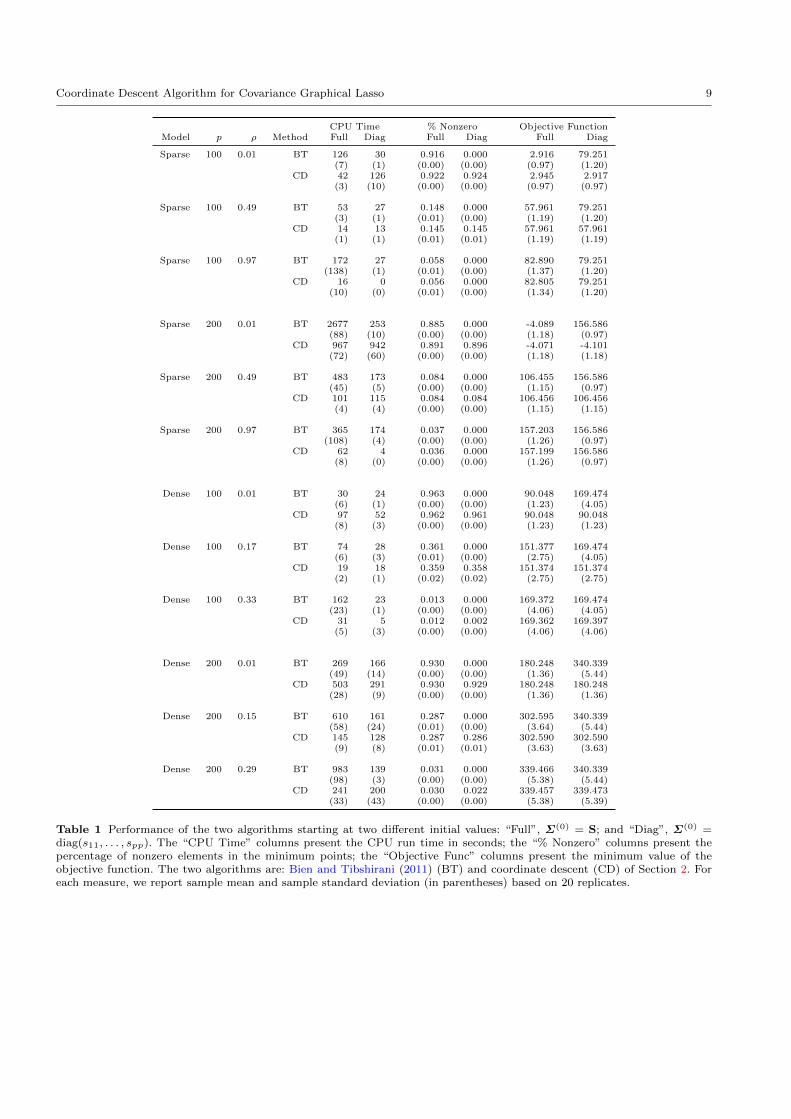
We record the CPU time, sparsity of the minimum

points and the minimum value of the objective func-

tion. Table 1 summarizes the observed values of these

measures based on 20 replicates by sample mean and

sample standard deviation. Three things are worth not-

ing. First, Bien and Tibshirani (2011)’s algorithm seems

to get stuck at the initial value of a diagonal matrix

in all cases. In contrast, the proposed algorithms work

fine and find reasonable minimum points of Σ, because

the minimum values of the objective function and the

level of sparsity are quite close to those obtained from

starting at the full sample covariance matrix. We have

also tried to initialize Bien and Tibshirani (2011)’s al-

gorithm at Σ(0)BT = diag(s11, . . . , spp)+10−3, but found

that it still gets stuck after a few iterations. Although

it may be possible to alleviate this issue by adjusting

some of Bien and Tibshirani (2011)’s algorithm’s tun-

ing parameters, it may be safe to conclude that Bien

and Tibshirani (2011)’s algorithm requires either very

careful tuning or performs badly at this important ini-

tial value. Second, initial values indeed matter. Com-

paring the results between full and diagonal initial val-

ues, we see substantial differences in all three measures.

For example, the limiting points from the diagonal ini-

tial matrices are sparser than those from the full initial

matrices. This is not surprising because of the drastic

difference in sparsity between these two starting points.

Third, comparing the minimum values of the objec-

tive function achieved by the two algorithms (last two

columns), we see that coordinate descent often finds

the smaller minimum values than Bien and Tibshirani

(2011)’s algorithms. The few exceptions seem to be the

cases when ρ is small and the fraction of the number of

non-zero elements is large.

4 Alternative algorithms

The coordinate descent algorithm described in Section

2 is indeed a cyclic algorithm because it systematically

cycles through coordinate directions to minimize the

lasso objection function (6). Although we have demon-

strated that it outperforms Bien and Tibshirani (2011)’s

algorithm, it is of interest to investigate whether this

cyclic coordinate descent algorithm can be further im-

proved by alternative algorithms. We propose and ex-

plore two additional competitors: a greedy coordinate

descent algorithm and a majorize-minimize MM algo-

rithm. We briefly describe these two algorithms below.

The greedy coordinate descent algorithm updates

along the coordinate direction that gives the largest gra-

dient descent. It has been implemented and explored,

for example, in nonparametric wavelet denoising models

(Sardy et al, 2000) and in l1 and l2 regressions (Wu and

Lange, 2008). In the covariance graphical lasso model,

we implement a version of the greedy coordinate de-

scent algorithm based on the theoretical results of di-

rectional derivatives (Wu and Lange, 2008) for identi-

fying the deepest gradient descent coordinate in each

iteration for solving (6).

The majorize-minimize MM algorithm is a general

optimization algorithm that creates a surrogate func-

tion that is easier to minimize than the original ob-

jection function (Hunter and Lange, 2004). The design

of the surrogate function is key to its efficiency. For

the covariance graphical lasso model, Bien and Tibshi-

rani (2011)’s MM algorithm uses a surrogate function

that is minimized by elementwise soft-thresholding. We

consider an alternative surrogate function that can be

minimized by updating one column and one row at a

time. The details of our new MM algorithm is provided

in Appendix.

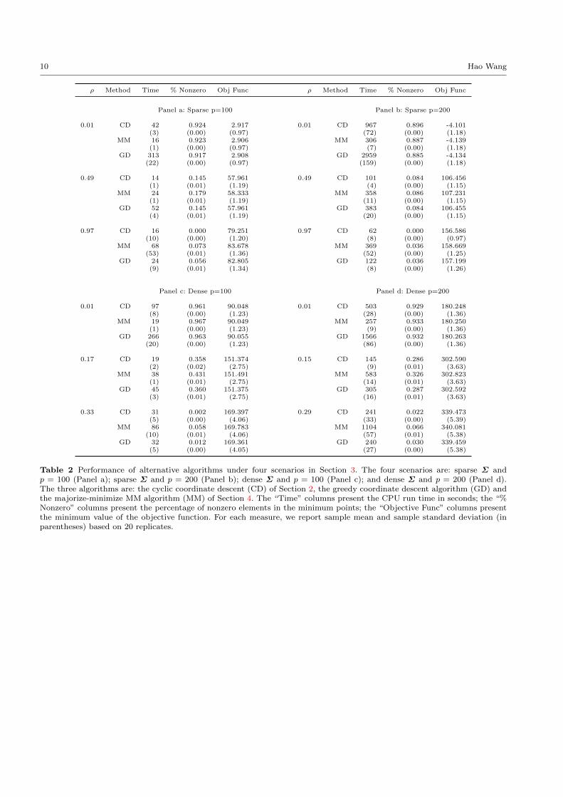
We use the greedy coordinate descent algorithm and

the new MM algorithm for fitting the covariance graph-

ical lasso model in the same experiment in Table 1. The

results are presented in Table 2. For easy comparison,

the results of the cyclic coordinate descent algorithm

in Table 1 is also shown. Only results from runs ini-

tialized at the sample covariance matrix are reported.

The relative performance of computing time from runs

Coordinate Descent Algorithm for Covariance Graphical Lasso 5

initialized at the diagonal covariance matrix is similar.

Comparing algorithms at a fixed ρ within each scenario,

we observe that the cyclic coordinate descent algorithm

is the fastest except when the shrinkage parameter is

tiny (i.e., ρ = 0.01) and the resulted estimate of Σ has a

high percentage of non-zero elements (i.e., about 90%).

In these exceptions, the new MM algorithm seems to

be the fastest. Since sparse estimates of Σ is more in-

teresting than dense estimates, the cyclic coordinate

descent algorithm is perhaps the most desirable algo-

rithm among the three. The greedy coordinate descent

algorithm is substantially slower than the cyclic coor-

dinate descent algorithm. This is consistent with Wu

and Lange (2008) which report a better performance of

the cyclic coordinate descent algorithm over the greedy

coordinate descent algorithm for fitting l2 regressions

under lasso penalty, and may indicate that the extra

computational cost of finding the deepest gradient de-

scent is not compensated by the reduced number of

iterations until convergence.

5 Discussion

We have developed a coordinate descent algorithm for

fitting sparse covariance graphical lasso models. The

new algorithm is shown to be much easier to implement,

significantly faster to run and numerically more stable

than the algorithm of Bien and Tibshirani (2011). Both

MATLAB and R software packages implementing the

new algorithms for solving covariance graphical mod-

els are freely available from the author’s website of the

paper.

Appendix

Details of the majorize-minimize MM algorithm in Sec-

tion 4

Consider√σ2ij + ε as an approximation to |σij | for a

small ε > 0. Consequently, the original objective func-

tion (1) can be approximated by

log(detΣ)+tr(SΣ−1)+2ρ∑i<j

√σ2ij + ε+ρ

∑i

σii. (9)

Note the inequality

√σ2ij + ε ≤

√(σ

(k)ij )2 + ε+

σ2ij − (σ

(k)ij )2

2√

(σ(k)ij )2 + ε

,

for a fixed σ(k)ij and all σij . Then (9) is majorized by

Q(Σ | Σ(k)) = log(detΣ) + tr(SΣ−1)

+ρ∑i<j

σ2ij√

(σ(k)ij )2 + ε

+ ρ∑i

σii. (10)

The minimize-step in MM then minimizes (10) along

each column (row) of Σ. Without loss of generality,

consider the last column and row. Partition Σ and S

as in (2) and consider the same transformation from

(σ12, σ22) to (β = σ12, γ = σ22 − σ′12Σ−111 σ12). The

four terms in (10) can be written as functions of (β, γ)

log(detΣ) = log(γ) + c1,

tr(SΣ−1) = β′Σ−111 S11Σ−111 βγ

−1 − 2s′12Σ−111 βγ

−1

+s22γ−1 + c2,

ρ∑i<j

σ2ij√

(σ(k)ij )2 + ε

= ρβ′D−1β, D = diag(

√(σ

(k)ij )2 + ε),

ρ∑i

σii = ρ(β′Σ−111 β + γ) + c3,

where c1, c2 and c3 are constants not involving (β, γ).

Dropping off c1,c2 and c3 from (10), we only have to

minimize

Q(β, γ | Σ(k)) = log(γ) + β′Σ−111 S11Σ−111 βγ

−1

−2s′12Σ−111 βγ

−1+s22γ−1+ρβ′D−1β+ρβ′Σ−111 β+ργ.

(11)

For γ, it is easy to derive from (11) that the conditional

minimum point given β is the same as in (5). For β,

(11) can be written as a function of β,

Q(β | γ,Σ(k)) = β′(V + ρD−1)β − 2u′β,

where V and u are defined in (6). This implies that the

conditional minimum point of β is β = (V+ρD−1)−1u.

Cycling through every column always drives down the

approximated objective function (9). In our implemen-

tation, the value of ε is chosen as follows. The approxi-

mation error of (9) to (1) is

2ρ∑i<j

(√σ2ij + ε− |σij |) = 2ρ

∑i<j

ε√σ2ij + ε+ |σij |

< 2ρ∑i<j

ε√ε

= ρp(p− 1)√ε.

Note that the algorithm stops when the change of the

objective function is less than 10−3. We choose ε such

that ρp(p−1)√ε = 0.001, i.e., ε = (0.001/(ρ(p−1)p))2,

to ensure that the choice of ε has no more influence on

the estimated Σ than the stoping rule.

6 Hao Wang

References

Bien J, Tibshirani RJ (2011) Sparse estimation of a

covariance matrix. Biometrika 98(4):807–820, DOI

10.1093/biomet/asr054

Breheny P, Huang J (2011) Coordinate descent algo-

rithms for nonconvex penalized regression, with ap-

plications to biological feature selection. The Annals

of Applied Statistics (1):232–253

Dempster A (1972) Covariance selection. Biometrics

28:157–75

Friedman J, Hastie T, Hfling H, Tibshirani R (2007)

Pathwise coordinate optimization. The Annals of Ap-

plied Statistics 1(2):pp. 302–332

Friedman J, Hastie T, Tibshirani R (2008) Sparse in-

verse covariance estimation with the graphical lasso.

Biostatistics 9(3):432–441

Fu WJ (1998) Penalized regressions: The bridge versus

the lasso. Journal of Computational and Graphical

Statistics 7(3):pp. 397–416

Hunter DR, Lange K (2004) A Tutorial on MM Al-

gorithms. The American Statistician 58(1), DOI

10.2307/27643496

Lin N (2010) A penalized likelihood approach in co-

variance graphical model selection. Ph.D. Thesis, Na-

tional University of Singapore

Sardy S, Bruce AG, Tseng P (2000) Block coordi-

nate relaxation methods for nonparametric wavelet

denoising. Journal of Computational and Graphical

Statistics 9(2):361–379

Tseng P (2001) Convergence of a block coordinate

descent method for nondifferentiable minimization.

Journal of Optimization Theory and Applications

109:475–494

Wu TT, Lange K (2008) Coordinate descent algorithms

for lasso penalized regression. The Annals of Applied

Statistics 2(1):pp. 224–244

Coordinate Descent Algorithm for Covariance Graphical Lasso 7

(a) (b)

(c) (d)

Fig. 1 CPU time is plotted against the shrinkage parameter ρ under four different scenarios for two algorithms. The x axisshows both the shrinkage parameter ρ and the average percentage of non-zero off-diagonal elements across the replicates atthat ρ (in parentheses). The y axis shows the computing time in seconds. The four scenarios are: sparse Σ and (p, n) =(100, 200) (Panel a); sparse Σ and (p, n) = (200, 400) (Panel b); dense Σ and (p, n) = (100, 200) (Panel c), and dense Σ and(p, n) = (200, 400) (Panel d). The two algorithms are: Bien and Tibshirani (2011) (BT, dashed gray line), and coordinatedescent (CD, solid black line). Each line represents results of one of the 20 replicates. Each computation is initialized at thesample covariance matrix Σ(0) = S.

8 Hao Wang

(a) (b)

(c) (d)

Fig. 2 Relative minimum value of the objective function, defined in (8), is plotted against the shrinkage parameter ρ underfour different scenarios for two algorithms. The x axis shows both the shrinkage parameter ρ and the average percentage ofnon-zero off-diagonal elements across the replicates at that ρ (in parentheses). The y axis shows the relative minimum valueof the objective function. The four scenarios are: sparse Σ and (p, n) = (100, 200) (Panel a); sparse Σ and (p, n) = (200, 400)(Panel b); dense Σ and (p, n) = (100, 200) (Panel c), and dense Σ and (p, n) = (200, 400) (Panel d). The two algorithms are:Bien and Tibshirani (2011) (BT, dashed gray line), and coordinate descent (CD, solid black line). Each line represents resultsof one of the 20 replicates. Each computation is initialized at the sample covariance matrix Σ(0) = S.

Coordinate Descent Algorithm for Covariance Graphical Lasso 9

CPU Time % Nonzero Objective FunctionModel p ρ Method Full Diag Full Diag Full Diag

Sparse 100 0.01 BT 126 30 0.916 0.000 2.916 79.251(7) (1) (0.00) (0.00) (0.97) (1.20)

CD 42 126 0.922 0.924 2.945 2.917(3) (10) (0.00) (0.00) (0.97) (0.97)

Sparse 100 0.49 BT 53 27 0.148 0.000 57.961 79.251(3) (1) (0.01) (0.00) (1.19) (1.20)

CD 14 13 0.145 0.145 57.961 57.961(1) (1) (0.01) (0.01) (1.19) (1.19)

Sparse 100 0.97 BT 172 27 0.058 0.000 82.890 79.251(138) (1) (0.01) (0.00) (1.37) (1.20)

CD 16 0 0.056 0.000 82.805 79.251(10) (0) (0.01) (0.00) (1.34) (1.20)

Sparse 200 0.01 BT 2677 253 0.885 0.000 -4.089 156.586(88) (10) (0.00) (0.00) (1.18) (0.97)

CD 967 942 0.891 0.896 -4.071 -4.101(72) (60) (0.00) (0.00) (1.18) (1.18)

Sparse 200 0.49 BT 483 173 0.084 0.000 106.455 156.586(45) (5) (0.00) (0.00) (1.15) (0.97)

CD 101 115 0.084 0.084 106.456 106.456(4) (4) (0.00) (0.00) (1.15) (1.15)

Sparse 200 0.97 BT 365 174 0.037 0.000 157.203 156.586(108) (4) (0.00) (0.00) (1.26) (0.97)

CD 62 4 0.036 0.000 157.199 156.586(8) (0) (0.00) (0.00) (1.26) (0.97)

Dense 100 0.01 BT 30 24 0.963 0.000 90.048 169.474(6) (1) (0.00) (0.00) (1.23) (4.05)

CD 97 52 0.962 0.961 90.048 90.048(8) (3) (0.00) (0.00) (1.23) (1.23)

Dense 100 0.17 BT 74 28 0.361 0.000 151.377 169.474(6) (3) (0.01) (0.00) (2.75) (4.05)

CD 19 18 0.359 0.358 151.374 151.374(2) (1) (0.02) (0.02) (2.75) (2.75)

Dense 100 0.33 BT 162 23 0.013 0.000 169.372 169.474(23) (1) (0.00) (0.00) (4.06) (4.05)

CD 31 5 0.012 0.002 169.362 169.397(5) (3) (0.00) (0.00) (4.06) (4.06)

Dense 200 0.01 BT 269 166 0.930 0.000 180.248 340.339(49) (14) (0.00) (0.00) (1.36) (5.44)

CD 503 291 0.930 0.929 180.248 180.248(28) (9) (0.00) (0.00) (1.36) (1.36)

Dense 200 0.15 BT 610 161 0.287 0.000 302.595 340.339(58) (24) (0.01) (0.00) (3.64) (5.44)

CD 145 128 0.287 0.286 302.590 302.590(9) (8) (0.01) (0.01) (3.63) (3.63)

Dense 200 0.29 BT 983 139 0.031 0.000 339.466 340.339(98) (3) (0.00) (0.00) (5.38) (5.44)

CD 241 200 0.030 0.022 339.457 339.473(33) (43) (0.00) (0.00) (5.38) (5.39)

Table 1 Performance of the two algorithms starting at two different initial values: “Full”, Σ(0) = S; and “Diag”, Σ(0) =diag(s11, . . . , spp). The “CPU Time” columns present the CPU run time in seconds; the “% Nonzero” columns present thepercentage of nonzero elements in the minimum points; the “Objective Func” columns present the minimum value of theobjective function. The two algorithms are: Bien and Tibshirani (2011) (BT) and coordinate descent (CD) of Section 2. Foreach measure, we report sample mean and sample standard deviation (in parentheses) based on 20 replicates.

10 Hao Wang

ρ Method Time % Nonzero Obj Func ρ Method Time % Nonzero Obj Func

Panel a: Sparse p=100 Panel b: Sparse p=200

0.01 CD 42 0.924 2.917 0.01 CD 967 0.896 -4.101(3) (0.00) (0.97) (72) (0.00) (1.18)

MM 16 0.923 2.906 MM 306 0.887 -4.139(1) (0.00) (0.97) (7) (0.00) (1.18)

GD 313 0.917 2.908 GD 2959 0.885 -4.134(22) (0.00) (0.97) (159) (0.00) (1.18)

0.49 CD 14 0.145 57.961 0.49 CD 101 0.084 106.456(1) (0.01) (1.19) (4) (0.00) (1.15)

MM 24 0.179 58.333 MM 358 0.086 107.231(1) (0.01) (1.19) (11) (0.00) (1.15)

GD 52 0.145 57.961 GD 383 0.084 106.455(4) (0.01) (1.19) (20) (0.00) (1.15)

0.97 CD 16 0.000 79.251 0.97 CD 62 0.000 156.586(10) (0.00) (1.20) (8) (0.00) (0.97)

MM 68 0.073 83.678 MM 369 0.036 158.669(53) (0.01) (1.36) (52) (0.00) (1.25)

GD 24 0.056 82.805 GD 122 0.036 157.199(9) (0.01) (1.34) (8) (0.00) (1.26)

Panel c: Dense p=100 Panel d: Dense p=200

0.01 CD 97 0.961 90.048 0.01 CD 503 0.929 180.248(8) (0.00) (1.23) (28) (0.00) (1.36)

MM 19 0.967 90.049 MM 257 0.933 180.250(1) (0.00) (1.23) (9) (0.00) (1.36)

GD 266 0.963 90.055 GD 1566 0.932 180.263(20) (0.00) (1.23) (86) (0.00) (1.36)

0.17 CD 19 0.358 151.374 0.15 CD 145 0.286 302.590(2) (0.02) (2.75) (9) (0.01) (3.63)

MM 38 0.431 151.491 MM 583 0.326 302.823(1) (0.01) (2.75) (14) (0.01) (3.63)

GD 45 0.360 151.375 GD 305 0.287 302.592(3) (0.01) (2.75) (16) (0.01) (3.63)

0.33 CD 31 0.002 169.397 0.29 CD 241 0.022 339.473(5) (0.00) (4.06) (33) (0.00) (5.39)

MM 86 0.058 169.783 MM 1104 0.066 340.081(10) (0.01) (4.06) (57) (0.01) (5.38)

GD 32 0.012 169.361 GD 240 0.030 339.459(5) (0.00) (4.05) (27) (0.00) (5.38)

Table 2 Performance of alternative algorithms under four scenarios in Section 3. The four scenarios are: sparse Σ andp = 100 (Panel a); sparse Σ and p = 200 (Panel b); dense Σ and p = 100 (Panel c); and dense Σ and p = 200 (Panel d).The three algorithms are: the cyclic coordinate descent (CD) of Section 2, the greedy coordinate descent algorithm (GD) andthe majorize-minimize MM algorithm (MM) of Section 4. The “Time” columns present the CPU run time in seconds; the “%Nonzero” columns present the percentage of nonzero elements in the minimum points; the “Objective Func” columns presentthe minimum value of the objective function. For each measure, we report sample mean and sample standard deviation (inparentheses) based on 20 replicates.