Coordinate free integrals in Geometric Calculus

Timo Alhoe-mail: alho@hi.is

Science Institute, University of IcelandDunhaga 5, 107 Reykjavik, Iceland

September 15, 2016

Abstract

We introduce a method for evaluating integrals in geometric calculuswithout introducing coordinates, based on using the fundamental theoremof calculus repeatedly and cutting the resulting manifolds so as to create aboundary and allow for the existence of an antiderivative at each step. Themethod is a direct generalization of the usual method of integration on R.It may lead to both practical applications and help unveil new connectionsto various fields of mathematics.

1

arX

iv:1

509.

0840

3v2

[m

ath.

DG

] 1

4 Se

p 20

16

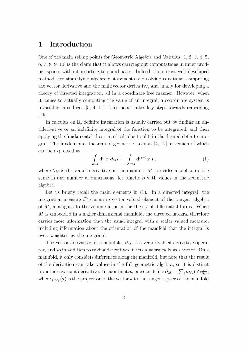
1 Introduction

One of the main selling points for Geometric Algebra and Calculus [1, 2, 3, 4, 5,6, 7, 8, 9, 10] is the claim that it allows carrying out computations in inner prod-uct spaces without resorting to coordinates. Indeed, there exist well developedmethods for simplifying algebraic statements and solving equations, computingthe vector derivative and the multivector derivative, and finally for developing atheory of directed integration, all in a coordinate free manner. However, whenit comes to actually computing the value of an integral, a coordinate system isinvariably introduced [5, 4, 11]. This paper takes key steps towards remedyingthis.

In calculus on R, definite integration is usually carried out by finding an an-tiderivative or an indefinite integral of the function to be integrated, and thenapplying the fundamental theorem of calculus to obtain the desired definite inte-gral. The fundamental theorem of geometric calculus [4, 12], a version of whichcan be expressed as ∫

M

dmx ∂MF =

∫∂M

dm−1x F, (1)

where ∂M is the vector derivative on the manifold M , provides a tool to do thesame in any number of dimensions, for functions with values in the geometricalgebra.

Let us briefly recall the main elements in (1). In a directed integral, theintegration measure dm x is an m-vector valued element of the tangent algebraof M , analogous to the volume form in the theory of differential forms. WhenM is embedded in a higher dimensional manifold, the directed integral thereforecarries more information than the usual integral with a scalar valued measure,including information about the orientation of the manifold that the integral isover, weighted by the integrand.

The vector derivative on a manifold, ∂M , is a vector-valued derivative opera-tor, and so in addition to taking derivatives it acts algebraically as a vector. On amanifold, it only considers differences along the manifold, but note that the resultof the derivation can take values in the full geometric algebra, so it is distinctfrom the covariant derivative. In coordinates, one can define ∂M =

∑i pMx(e

i) ∂∂xi

,where pMx(a) is the projection of the vector a to the tangent space of the manifold

2

at point x. In what follows, we usually suppress x in the notation, and also Mwhere the manifold is clear from context.

Let us present a summary of the method we are proposing, to be elabo-rated on in the rest of the paper: assume we are integrating a function f(x)

over a d-dimensional subset M of Rd, which is sufficiently smooth to satisfythe assumptions of the fundamental theorem and has a finite number of con-nected components. The first step is to find an antiderivative F1(x) of f(x), i.e.∂MF1(x) = f(x) for all x ∈ M . Now we get, according to (1), an integral overthe d−1 dimensional boundary ∂M of M . We’d like to use the fundamental the-orem again, and so we look for an antiderivative F2(x) of F1(x) on the boundary∂M with respect to the derivative ∂∂M on the boundary. Given an antiderivativeF2(x) we run into the problem that the boundary of the boundary of a set isalways empty. We move forward by making an incision of the boundary, i.e. wechoose a set E2 such that ∂M \E2 has a smooth boundary ∂E2∂M := ∂(∂M \E2),and vol(E2) < ε2. Now the integral∫

∂E2∂M

dd−2xF2(x) (2)

differs from our desired integral by at most vol(E2) supx∈E2

∥∥F2(x)∥∥. Notice that

we have to choose F2 and E2 such that F2 is continuous in ∂M \ E2, in order tojustify our use of the fundamental theorem. This requirement is actually crucial,since any finite value of the integral as we shrink ε2 to zero comes from what areessentially branch cut discontinuities in the antiderivative. Indeed, due to thepresence of branch cuts, we could not have found F2(x) on the whole manifold,giving a second reason why the incision is necessary.

We then simply repeat the same construction d times, at each step requiringthat for incision En the volume vol(En) < εn and that each antiderivative iscontinuous in the integration set. In the final step, the integration will be overa one-dimensional manifold, which simply has a finite number of points as aboundary, leaving us with a finite sum of values of the dth antiderivative. Thenas we let all of the εn’s go to zero, we get our final result.

As will be shown via examples, this method allows computing integrals with-out invoking a coordinate system. However, we will find in all practical examplesthat we do need to invoke reference vectors or multivectors, and the expectation is

3

indeed that this will turn out to be generic, as the reference multivectors providea mechanism for choosing a specific antiderivative.

We expect that this method of integration will open up new possibilities inanalyzing any integral or differential systems in n-dimensions. This includesthe theory of partial differential equations1, numerical estimation methods forintegrals, and also connections to algebraic geometry, since it becomes possible,at least in principle, to handle all aspects of surfaces expressible as algebraicequations in a coordinate independent manner.

In this paper, we first prove that when the requisite antiderivatives and sub-manifolds exist and satisfy a number of reasonable properties, the above construc-tion indeed gives the desired result. We then give some examples of elementaryintegrals worked out according to the method. Finally, we elaborate on possibleimplications and directions for further research.

2 Integration by antiderivatives

Let us briefly recall some definitions and establish some notation.Our basic notation follows that used by [13]. We use the left- and right con-

tractions b and c instead of the single dot product, our scalar product contains thereverse, A∗B = 〈AB〉, and our dual is a right multiplication by the pseudoscalar.The norm on a geometric algebra is defined as ‖A‖2 = A ∗ A = 〈AA〉. Althoughour method generalizes easily to the case of mixed signatures, we will for simplic-ity consider here only spaces where the inner product is positive definite, and sothe multivector norm defines a well-behaved concept of convergence.

Since the directed integral of a multivector function can always be expandedin a multivector basis in terms of scalar coefficient functions, we can import theconcept of integrability from scalar valued integrals:

Definition 1. A function f : M → GM(x) is L-integrable in the sense of thedirected integral on M if each of the scalar functions aI(x) ∗ ( dm x

‖dm x‖f(x)) are L-integrable on M with the measure‖dm x‖ for all aI , where I is a multi-index andthe set {aI(x)} forms a multivector basis [4, 13] of GM(x), and L is a definitionof integrability for scalar valued functions, such as Riemann or Lebesgue.

1 When such equations are expressed in geometric calculus, we follow [4] in considering thisa misnomer, and prefer the term vector differential equation.

4

In what follows, we will simply refer to integrability, and by that mean in-tegrability in the sense of the directed integral based on a suitable definition ofscalar integrability. For all the theorems and examples in this paper, the Riemannintegral will be sufficient.

We write vol(M) for the volume of a manifold in the appropriate dimension,i.e. for dim(M) = 2 the volume is the area, and so on.

For completeness, let us recall the definition of the tangent algebra and thevector derivative [4]:

Definition 2. Let M be a Euclidean vector manifold [4]. Then the tangentalgebra of M at x ∈ M , denoted by GM(x) is the geometric algebra, i.e. realClifford algebra, generated by the tangent space TxM .

Definition 3. Given a vector derivative ∂M on an orientable vector manifold Mand an orientable submanifold N ⊆ M and a unit pseudoscalar of N , IN(x) ∈GM(x), for each x ∈ N , the projected derivative ∂N is given by [4]

∂N = pNx(∂) =∑i

pNx(ei)ei · ∂M =∑i

pNx(ei)∂

∂xi, (3)

where pNx(a) = IN(x)−1(IN(x) b a) is the projection of a vector a to the tangent

algebra of the manifold N at x ∈ N , and {ei} is a basis of the tangent spaceTxM .

Note that the partial derivative operator does not operate on the pseudoscalarIN(x), and also that the projected derivative can take values in the full tangentalgebra of M , not just N . In addition, the projections on the basis vectors ei canbe dropped if we let the sum run only over a basis of TxN . Then one version ofthe fundamental theorem of calculus can be expressed as [4, 12]

Theorem 1 (Fundamental theorem of calculus). LetM be an orientedm-dimensionalvector manifold with pseudoscalar IM(x) and a boundary ∂M that is a vector man-ifold, f a differentiable function f : M → GM(x), and ∂M the vector derivativeon M . Then ∫

M

dmx ∂Mf(x) =

∫∂M

dm−1x f(x), (4)

where the pseudoscalar dm−1x is oriented such that IM(x)∥∥dm−1x∥∥ = dm−1x n(x),

where n(x) is the outward directed unit normal of ∂M at x.

5

Note that since the measure is pseudoscalar-valued, its position relative to theintegrand matters. Indeed, the most general form of the theorem is concernedwith integrals of the form

∫L(dmx), where L(dmx) is a linear function of dmx

[4]. However, we will only consider the form with the pseudoscalar measure tothe left of the integrand in this paper. Let us point out some consequences of therequirement concerning the orientation of the pseudoscalar of ∂M :

• when we make a very small incision on a manifold, the pseudoscalars of thenewly created boundary at two nearby points x1 and x2, on opposite sidesof the incision, will be related by I(x1) ≈ −I(x2), since the correspondingoutward normals will be nearly opposite. This is what guarantees, at thelevel of the fundamental theorem, that small incisions in a region where theantiderivative is continuous have a small effect on the value of the integral.

• whenM is a 1-dimensional manifold, so that its pseudoscalar dx is a vector,then the unit pseudoscalar of ∂M , d0x, is the scalar ±1. Indeed, onecan think of d0x as a signed counting measure. As the direction of dx

is continuous over the curve, this sign will specifically be +1 at one of theendpoints and −1 at the other, in accordance with the fundamental theoremof calculus on R.

Let us then prove a simple lemma:

Lemma 2. Let M be an oriented m-dimensional vector manifold and f : M →GM(x) be an integrable function from the manifold to the algebra. Given a boundedsubmanifold E ⊂M such that f is bounded in E, then∥∥∥∥∥

∫M\E

dm x f(x)−∫M

dm x f(x)

∥∥∥∥∥ ≤ vol(E) supx∈E

∥∥f(x)∥∥ (5)

Proof. Direct calculation using the triangle inequality:∥∥∥∥∥∫M\E

dm x f(x)−∫M

dm x f(x)

∥∥∥∥∥ =

∥∥∥∥∫E

dm x f(x)

∥∥∥∥ ≤ ∫E

∥∥dm x f(x)∥∥=

∫E

‖dm x‖∥∥f(x)∥∥ ≤ ∫

E

‖dm x‖ supx∈E

∥∥f(x)∥∥ = vol(E) supx∈E

∥∥f(x)∥∥ . (6)

6

Note that the suprema exists and is finite since E is bounded and f is boundedon E.

The point of Lemma 2 is that it allows us to cut out a part of the manifold inorder to guarantee that it has a boundary, and still keep control of the error weare making. Also, we will find out that usually functions on manifolds withoutboundary do not have single valued antiderivatives, and the lemma allows us toexclude a branch cut, since the existence of the antiderivative is only necessaryon the part of the manifold that is not cut.

Definition 4. Let M be a vector manifold and f : M → GM(x) be a functionon the manifold. If f has an antiderivative F on M , we write F =: ∂−1M f . If∂−1M f again has an antiderivative on N ⊆ M , we denote that by ∂−2MNf , and ingeneral we write ∂−nM1M2...Mn

f for the nth antiderivative of f on the manifold Mn,if it exists, with M1 ⊆M2 ⊆ . . . ⊆Mn.

Note that due to the projection operator in the derivative on a manifold, theantiderivative in general depends on the manifold in which it is defined. In otherwords an antiderivative on a submanifold is not necessarily just the restrictionof some antiderivative on the full manifold. Also, in the above definition theantiderivative is ambiguous, so when using the notation we have to either definehow to choose a specific antiderivative, or show that our results don’t depend onthe choice.

Now we get to the main result:

Theorem 3. Let M be an m-dimensional orientable vector manifold, and f :

M → GM(x) an integrable function. If there exists a sequence of orientablemanifolds N0 ⊂ N1 ⊂ . . . ⊂ Nm = M and a sequence of bounded sets Ei suchthat

• if ∂Ni+1 6= ∅, Ni = ∂Ni+1, otherwise Ni = ∂(Ni+1 \ Ei+1), where Ei+1 isa bounded set such that the boundary ∂(Ni+1 \Ei+1) is a non-empty vectormanifold, and ∂−m+i+1

Ni+1...Nmf is integrable and bounded on Ei+1.

• there exists an antiderivative ∂−m+iNi...Nm

f on Ni, which is bounded.

• N0 is a finite set

7

then the integral of f overM can be computed by evaluating the mth antiderivativeon N0: ∥∥∥∥∥∥

∫M

dm x f(x)−∑xi∈N0

∂−mN0...Nmsif(xi)

∥∥∥∥∥∥ ≤ ε, (7)

where ε = maxi supx∈Ei

∥∥∥∂−m+iNi...Nm

f(x)∥∥∥∑i vol(Ei), and the signs si ∈ {−1, 1} are

determined by fulfilling the requirement on the orientation of the boundary in thefundamental theorem at each step.

Before proving the theorem, we make a few remarks. We basically forcedthe theorem to be true by sticking all the difficult parts into the assumptions.Note however that the local existence of an antiderivative is guaranteed for adifferentiable function [11, 14, 12], and also that the set N0 is automaticallydiscrete since it is the boundary of a 1-dimensional manifold, and with very mildassumptions on M the Ei can be chosen such that N0 is a finite set. In essencethese assumptions allows us to prove the theorem without getting mixed up intopological complications, and for most practical applications the natural choiceof the sets Ni will anyway fulfill these assumptions, which is why we are notinterested in sharpening the theorem at this point.2

Proof of theorem 3. First note that since the integral of a bounded function overa bounded set is finite, each of the suprema in the expression for ε exist. The onlypart left to prove is the inequality. Using the fundamental theorem, Lemma 2

2 Since in many applications there may be a branch cut that goes to infinity, relaxingthe assumption about Ei’s being bounded would be beneficial, allowing to compute also suchintegrals when they are finite. This would entail finding a sufficient set of assumptions toguarantee that

∫Ei

∂−m+iNi...Nm

f goes to zero as the set Ei shrinks to zero. In specific cases thisshould not be difficult.

8

and the triangle inequality, we first compute∥∥∥∥∥∥∫M

dm x f(x)−∑xi∈N0

∂−mN0...Nmsif(xi)

∥∥∥∥∥∥=

∥∥∥∥∥∫M

dm x f(x)−∫N1\E1

dx∂−m+1N1...Nm

f(x)

∥∥∥∥∥=

∥∥∥∥∥∫M

dm x f(x)−∫N1\E1

dx∂−m+1N1...Nm

f(x)

+

∫N1

dx∂−m+1N1...Nm

f(x)−∫N1

dx∂−m+1N1...Nm

f(x)

∥∥∥∥∥≤

∥∥∥∥∥∫M

dm x f(x)−∫N1

dx∂−m+1N1...Nm

f(x)

∥∥∥∥∥+

∥∥∥∥∥∫N1\E1

dx∂−m+1N1...Nm

f(x)−∫N1

dx∂−m+1N1...Nm

f(x)

∥∥∥∥∥≤

∥∥∥∥∥∫M

dm x f(x)−∫N1

dx∂−m+1N1...Nm

f(x)

∥∥∥∥∥+ vol(E1) sup

x∈E1

∥∥∥∂−m+1N1...Nm

f(x)∥∥∥ .

(8)

Note that since two antiderivatives differ at most by a monogenic function ψfor which ∂N0ψ(x) = 0 [4], this result is independent of the choice of antideriva-tive, resolving the caveat mentioned in definition 4. Also, the signs si mustindeed follow the orientation requirement of the fundamental theorem to allowrepresenting the sum as an integral.

We can then continue using similar steps, each of which produces an approx-imation error vol(Ei) supx∈Ei

∥∥∥∂−m+iNi...Nm

∥∥∥, until finally at the m’th step, we get

∥∥∥∥∥∫M

dm x f(x)−∫Nm

dm x ∂0Nmf(x)

∥∥∥∥∥+∑i

vol(Ei) supx∈Ei

∥∥∥∂−m+iNi...Nm

f(x)∥∥∥ , (9)

where Nm = M and ∂0Mf(x) is the function itself, and so the integral term iszero. Approximating the suprema by their maximum concludes the proof.

9

There is a simple corollary;

Corollary 4. Let M be a vector manifold without a boundary, and f : M →GM(x) be a bounded integrable function such that its integral over M is non-zero.Then any antiderivative ∂−1M f of f must have a branch cut discontinuity whichdivides the manifold into at least two parts with non-zero volumes.

Proof. Assume the opposite, that is, that there exists an antiderivative of f on thewhole of M . Then we can make a cut according to theorem 3, and let its volumeshrink to zero. Since the antiderivative of a bounded function is bounded (whichcan be seen, for example, by considering the scalar components and applying theusual theorems of integration), this means that the result of the integration iszero. This is a contradiction.

In particular, this means that the norm of the volume form on a manifoldwithout boundary cannot have an antiderivative everywhere. Also, since everyfunction on a manifold is an antiderivative of its own derivative, this corollarymay have some links to the hairy ball theorem.

Note also that even though the method is phrased in terms of the directedintegral, it is immediately applicable to the usual integral with a scalar measure.We simply write‖dm x‖ f(x) = dm xI(x)f(x), where I(x) is the unit pseudoscalarof the manifold at x.

In order to do a specific calculation, we find the necessary antiderivatives andsets to cut out by any means we like, and then using theorem 3, we can be assuredthat as we let the volume of the incisions Ei go to zero we get the exact valueof the integral. Note that since the errors are additive, the order of the limitsfor the various sets does not matter (unless their construction dictates a specificorder). Of course, we have only proven that if this construction can be made,then we can do the coordinate free integral. Let us next present some examplesto show that such constructions indeed do exist.

3 Examples

Next we compute examples of applying this method of integration. Since thesequite trivial examples already show many of the features we expect to encounter

10

in more generic cases, we work them out in detail. The algebra and rules forcomputing the derivatives needed in this section are contained, for example, in[4, 5, 15, 13].

3.1 The area of a disk

As the first example of application of the method, we calculate the area of a diskof radius r in R2. The integral we intend to compute is

ABr =

∫Br

d 2x, (10)

where Br = {x ∈ R2 : ‖x‖ < r}. Note that since the directed volume elementd 2x is a bivector, we expect to get the result as a bivector. We define thecorresponding unit bivector I2 = d 2x

‖d 2x‖ . The first step is to find the antiderivative

of the constant function 1. This is by inspection 12x, since in general the derivative

∂Mx ism, wherem is the dimension of the manifold [4, 15]. Therefore, the integralis reduced to

1

2

∫S1

dx x, (11)

where dx is the vector-valued measure on the circle. Now the projection ofa vector a to S1 at point x is pS1(a) = x−1(x ∧ a). Intuitively, we see thatthe integral to calculate measures distance along the circle, i.e. the angle. Sodoes the complex logarithm, and so we are led to the try the function log(xx0),where x0 is an arbitrary constant vector in G(R2), and since xx0 is in the evensubalgebra of G(R2) which is isomorphic to the complex numbers with the unitpseudoscalar x∧x0

‖x∧x0‖ = −I2 acting as the imaginary unit, the logarithm may bedefined analogously to the complex logarithm. The negative sign appears whencomparing the orientation of d 2x to that of x ∧ x0 via the requirement dx x =

‖dx‖ d 2x, coming from the fundamental theorem, where x is the unit normal atx, and choosing the positive sense of rotation to be counterclockwise.

In order to compute the projected derivative, we observe that in general∂Mf(x) = ∂M(a c ∂x)f(x), where ∂x is the full vector derivative without theprojection, and the overdot denotes that the derivative ∂M acts only on a. Then,using the chain rule and the fact that the derivative (xx0) ∗ ∂z reduces to the

11

directed derivative in the direction xx0 [15], which further reduces to the com-plex derivative times xx0 since the direction commutes with the argument, wecan further calculate

∂S1 log(xx0) = ∂S1(xx0) ∗ ∂z log z|z=xx0 = ∂S1(xx0)z−1|z=xx0

= x0x0x

‖xx0‖2= x−1,

(12)

where the overdot limits the scope of the derivative to the dotted objects, as in[4]. We observe that ∂S1x2 = 0, as expected, and therefore deduce immediatelythat ∂S1

12x2 log(xx0) = 1

2x, which is our antiderivative. The boundary of S1 is

empty, but according to our method we cut a small segment, for example the partwhere |x·x0|‖xx0‖ > cos ε which is the part at an angle less than ε to x0. The complexlogarithm function is bounded away from zero, and our incision is bounded, sothe assumptions of theorem 3 are satisfied and we calculate∫

S1

dx1

2x =

∑xi∈∂(S1\{x: ‖x−x0‖<ε})

si1

2x2i log(xix0). (13)

Let us choose the branch of the complex logarithm such that log(xx0)|x=x0 =

log‖xx0‖−0I2. We observe that since the antiderivative must be continuous insidethe set where we made the cut, we must then allow the logarithm to approach thevalue log‖xx0‖−2πI2 on the other side of the cut, where the negative sign comesfrom the sign difference between I2 and x ∧ x0. Note that this puts the branchcut on the positive real axis on the complex plane spanned by 1 and I2. Thesigns si are fixed by the fundamental theorem: at the beginning of the interval,dx points to the outside of the region, so the "pseudoscalar" must be s0 = 1 tokeep the outward unit normal in the same direction. At the end of the intervaldx points in the inward direction, and we get s1 = −1. Therefore the sum resultsin ABr = πr2I2, as expected.

12

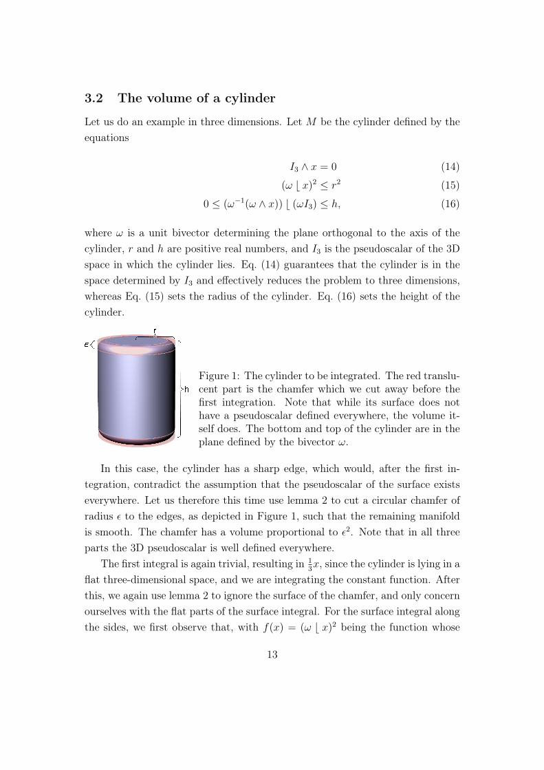
3.2 The volume of a cylinder

Let us do an example in three dimensions. Let M be the cylinder defined by theequations

I3 ∧ x = 0 (14)

(ω b x)2 ≤ r2 (15)

0 ≤ (ω−1(ω ∧ x)) b (ωI3) ≤ h, (16)

where ω is a unit bivector determining the plane orthogonal to the axis of thecylinder, r and h are positive real numbers, and I3 is the pseudoscalar of the 3Dspace in which the cylinder lies. Eq. (14) guarantees that the cylinder is in thespace determined by I3 and effectively reduces the problem to three dimensions,whereas Eq. (15) sets the radius of the cylinder. Eq. (16) sets the height of thecylinder.

Figure 1: The cylinder to be integrated. The red translu-cent part is the chamfer which we cut away before thefirst integration. Note that while its surface does nothave a pseudoscalar defined everywhere, the volume it-self does. The bottom and top of the cylinder are in theplane defined by the bivector ω.

In this case, the cylinder has a sharp edge, which would, after the first in-tegration, contradict the assumption that the pseudoscalar of the surface existseverywhere. Let us therefore this time use lemma 2 to cut a circular chamfer ofradius ε to the edges, as depicted in Figure 1, such that the remaining manifoldis smooth. The chamfer has a volume proportional to ε2. Note that in all threeparts the 3D pseudoscalar is well defined everywhere.

The first integral is again trivial, resulting in 13x, since the cylinder is lying in a

flat three-dimensional space, and we are integrating the constant function. Afterthis, we again use lemma 2 to ignore the surface of the chamfer, and only concernourselves with the flat parts of the surface integral. For the surface integral alongthe sides, we first observe that, with f(x) = (ω b x)2 being the function whose

13

constant value surface f(x) = r2 defines the side of the cylinder, and given apoint x on the side, the projection of a vector a to the tangent space is given by

pside(a) = (∂f(x)I3)−1(∂f(x)I3) b a = rω(a) + pxcω(a), (17)

whererω(a) = ω−1(ω ∧ x) and pxcω(a) = (x c ω)−1(x c ω) b a (18)

are the rejection from, i.e. part orthogonal to, ω, and the projection to thedirection of the vector x c ω, which lies in the plane of ω and orthogonal to x,respectively.

We find the antiderivative ∂−1sidex = x rω(x). This can be verified by takingthe derivative and using the facts that x = pω(x) + rω(x), where pω(x) is theprojection to ω, the fact that since the projection to the tangent space splitsas in Eq. (17) then also the derivatives split in the same way, and finally that∂px ∧ a = dpa − p(a), where ∂p is the derivative projected with the projection pand dp is the dimension of the subspace projected to.

In order to do the final integral for the side along the boundary left by thechamfer cut, which is a circle in the plane ω, and at height h − ε above theorigin, we note that rω(x) is simply the constant vector height along the circleand therefore also constant with respect to the derivative on that circle, so we areleft with integrating x = pω(x)+rω(x) on the circle. Now pω(x) is on the plane ofthe circle, and therefore we know from the disk example that the integral of thepω(x) -part will be 2π

∥∥pω(x)∥∥2 I2 with I2 = ω and∥∥pω(x)∥∥2 = r2. Integrating the

constant produces x times the constant, and since x is regular on the whole circle,the subtraction will produce 0. The other boundary component is the circle alongthe bottom, where the calculation is identical expect that now

∥∥rω(x)∥∥ = ε, andthe sign is opposite since the orientation of the boundary is opposite. The integralalong the sides then total 2π

3r2(h− 2ε)I3, where the pseudoscalar I3 comes from

the product of the bivector ω and vector rω(x).The other boundary components are the caps on the top and the bottom.

The projection to the tangent plane is simply pω, and therefore splitting againx = pω(x) + rω(x), we find the antiderivative

∂−1ω x =1

2pω(x)

2 +1

2pω(x)rω(x). (19)

14

The half on the second term comes from the fact that the projection is two-dimensional. We have to integrate this on the boundary of the cap, which is thecircle at radius r− ε (since we cut the chamfer off the edge). The first term againintegrates to zero, since on the circle (pω(x))

2 is a constant, whereas the secondterm again reduces to the case of the disk, and therefore produces π

3(r−ε)2ωrω(x),

where we have inserted the 1/3 from the first integral. The cap on the bottom isagain the same, with this time

∥∥rω(x)∥∥ = ε, and so putting the caps and the sidetogether and letting ε→ 0 we get the final result∫

cylinderd 3 x = πr2hI3 (20)

as expected.

4 Toward a more systematic method

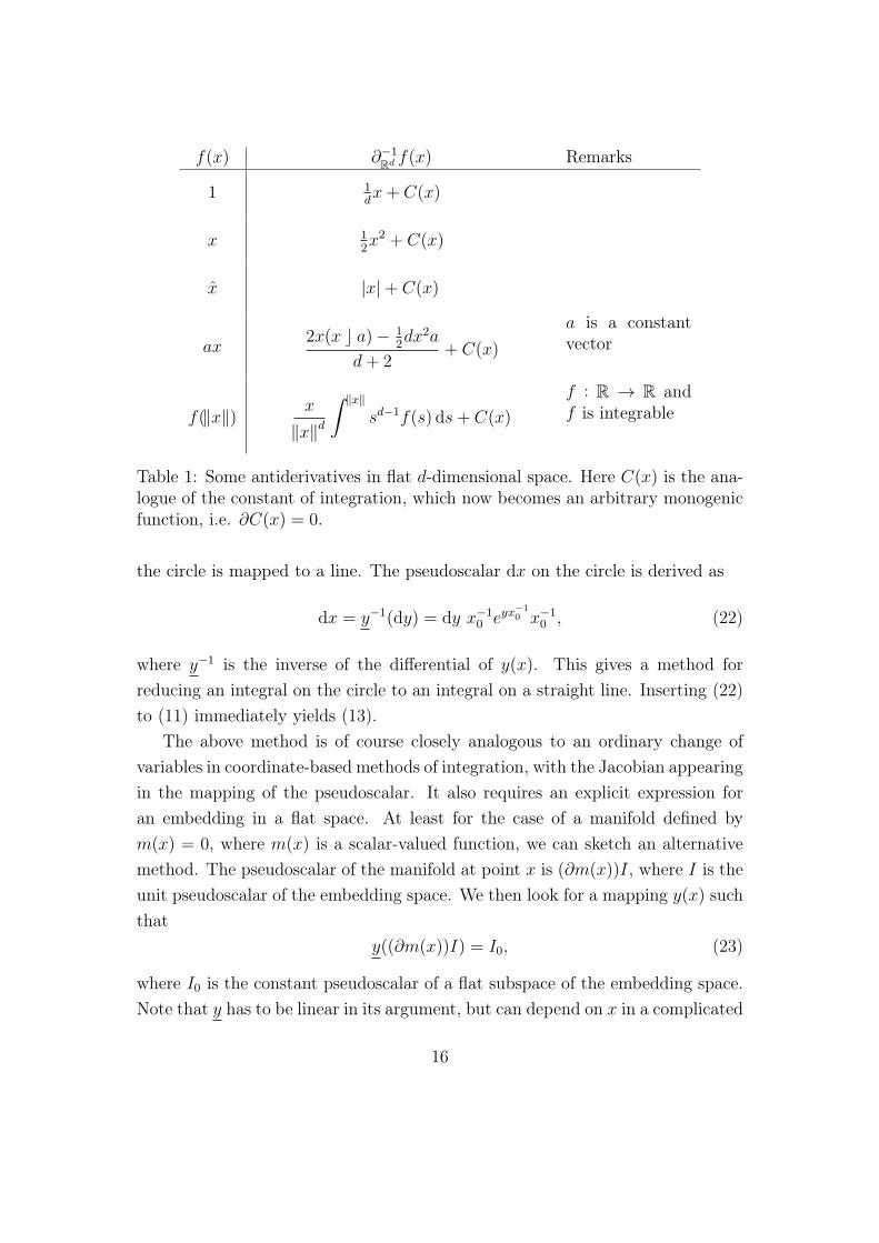
The above examples are calculated rather ad hoc, in the sense that the antideriva-tives are guessed and then checked by derivation. The path toward a more sys-tematic method for calculating coordinate-free integrals is however clear: first, asystematic table of antiderivatives needs to be built by reading tables of vectorderivatives in inverse. To provide an example, table 1 lists some such antideriva-tives. Once such a table exists in flat space, there is no need to generate a newone for each manifold. Rather, given a function on a manifold with a known em-bedding in flat space, we can simply use (the inverse of) the embedding functionto map the function to a flat subspace of the embedding manifold. The changeof variables induces a mapping of the pseudoscalar via its differential outermor-phism [4], from which we extract the pseudoscalar of the flat space. The productof the part extracted from the pseudoscalar and the function mapped to the flatsubspace can then be integrated using the table of antiderivatives in flat space.

For example, when integrating a function on the circle, the mapping

y(x) = log(xx0)x0 (21)

takes x to a vector y, with a constant length in the direction of x0, and changesin x along the circle affect y only in a direction orthogonal to x0. In other words,

15

f(x) ∂−1Rd f(x) Remarks

1 1dx+ C(x)

x 12x2 + C(x)

x |x|+ C(x)

ax2x(x c a)− 1

2dx2a

d+ 2+ C(x)

a is a constantvector

f(‖x‖) x

‖x‖d

∫ ‖x‖sd−1f(s) ds+ C(x)

f : R → R andf is integrable

Table 1: Some antiderivatives in flat d-dimensional space. Here C(x) is the ana-logue of the constant of integration, which now becomes an arbitrary monogenicfunction, i.e. ∂C(x) = 0.

the circle is mapped to a line. The pseudoscalar dx on the circle is derived as

dx = y−1(dy) = dy x−10 eyx−10 x−10 , (22)

where y−1 is the inverse of the differential of y(x). This gives a method forreducing an integral on the circle to an integral on a straight line. Inserting (22)to (11) immediately yields (13).

The above method is of course closely analogous to an ordinary change ofvariables in coordinate-based methods of integration, with the Jacobian appearingin the mapping of the pseudoscalar. It also requires an explicit expression foran embedding in a flat space. At least for the case of a manifold defined bym(x) = 0, where m(x) is a scalar-valued function, we can sketch an alternativemethod. The pseudoscalar of the manifold at point x is (∂m(x))I, where I is theunit pseudoscalar of the embedding space. We then look for a mapping y(x) suchthat

y((∂m(x))I) = I0, (23)

where I0 is the constant pseudoscalar of a flat subspace of the embedding space.Note that y has to be linear in its argument, but can depend on x in a complicated

16

way. Then (23) is a differential equation for the mapping which, once solved fora given manifold, reduces integrals of functions on the manifold to integrals on aflat space.

Finally, as already integrals of functions of a real variable can rarely be evalu-ated analytically in terms of a finite set of elementary functions, we cannot expectto do any better in this generalized case. Therefore the ultimate goal must be acoordinate-free approximation theory, which would allow evaluating integrals ofsufficiently smooth functions in a similar way as an integral for a real analyticfunction can always be evaluated in terms of a Taylor series. We however leavethat problem for a later work, although with some speculation about possibleproperties of such approximations in the next section.

5 Conclusions and outlook

We have presented a method for computing integrals in m dimensions withoutusing coordinates. Naturally, the level of freedom from using coordinates dependson how the manifold and the integrand are defined. One purely coordinate freeway is to define the manifold by solutions of m(x) = 0, where m(x) is a functionof the vector x constructed from geometric products of x with itself and some(possibly infinite) set of constant multivectors Ai, where the geometric relationsbetween Ai and x are known in sufficient detail to allow carrying out all thenecessary algebraic manipulations without coordinates. Both of our examplesare of this form.

In the examples, we integrate the constant function on two manifolds in or-der to compute their volumes. The actual computations in these examples arenot complicated when compared to the same computation in coordinates, whichfor a fair comparison needs to take into account the derivation of the Jacobianin polar or cylindrical coordinates. Further development of our method will in-deed require building a comprehensive toolbox of systematic methods for findingantiderivatives of multivector valued functions of vector variables on vector man-ifolds. While this program is still in its infancy, we have found some rules withsome level of generality: for example, as shown in table 1, an antiderivative off(‖x‖) in d-dimensions is simply x

‖x‖d∫ds sd−1f(s), where f(s) is a scalar valued

function of a scalar, and so the remaining integral is an ordinary scalar integral.

17

This rule is of course equivalent to integrating in a spherical coordinate system,expressed in a coordinate-free way.

As an interesting note, in some examples which we have worked out but notreported here, such as the volume of B3, it is not necessary to actually find anantiderivative, but rather one can find a function whose derivative differs from thedesired one by a function which can be seen to integrate to zero. We can then usesuch a function instead of the antiderivative to still get the correct result. How-ever, we will not comment on this further before we understand the phenomenonin more detail. It may turn out to be only a fortunate coincidence occurring in alimited number of cases, rather than something that can be included in a generaltoolbox.

Let us indulge in some speculation concerning possible applications of themethod to more than just evaluating integrals in the few special cases whereantiderivatives can be explicitly found. Consider a function f(x) on a manifoldM defined by m(x) = 0 for some multivector valued function m(x) and with xin Rd. In order to calculate the integral of f(x) over M , the method involvesfinding the d-fold antiderivative of f with respect to derivatives projected onM , and evaluating it on a discrete set of points on the manifold. Therefore,at least in the final step, we only really need to know some topological factsabout the manifold in order to choose the points such that they are all on thesame branch of the antiderivative. Of course, the manifold also enters into thecalculation via the projections of the derivative operator. For the first integrationin the case where m(x) is scalar-valued the projected derivative is given simplyby (∂m(x)Id)

−1(∂m(x)Id) b ∂, where the first two ∂ ’s affect only the m(x) ’simmediately following them. Similar formulas can be worked out for more generalm(x). Now, we can use the Taylor series approximation for multivector functions[15] and approximate both functions f(x) and m(x) by their Taylor series. Ifthe antiderivatives of all the monomial terms3 can be explicitly constructed, thenthis should in principle allow for a systematic series expansion for the values ofintegrals on a large class of manifolds, in terms of integrals of the monomials.The theoretical connections to algebraic geometry and topology should prove

3 We need to also expand the inverse appearing in the projection, or to integrate a rationalfunction of multivectors, which cannot be done in quite closed form even for the real numbers,as the roots of the polynomials need to be found in the partial fraction expansion.

18

interesting.For (vector) differential equations the very same rules for finding antideriva-

tives that are crucial for our method will be useful in finding closed form solutionsin a coordinate invariant way. In addition, similar series expansion methods asthose outlined above should pave the way to finding series expansions for solutionsof vector differential equations, and may even aid in their numerical evaluation.

On a philosophical level, our method represents a further step into the di-rection of establishing multivectors as geometric numbers, which can indeed beconstructed, manipulated and interpreted in a wholly coordinate-free way.

Acknowledgements

We thank A. Lewandowski and L. Thorlacius for very helpful comments andproofreading of the manuscript. The author is supported in part by IcelandicResearch Fund grant 130131-053 and by a grant from the University of IcelandResearch Fund.

References

[1] D. Hestenes, “Oersted Medal Lecture 2002: Reforming the mathematical languageof physics”, Am. J. Phys 71, 104 (2003),http://geocalc.clas.asu.edu/pdf/OerstedMedalLecture.pdf.

[2] D. Hestenes, “Spacetime Physics with Geometric Algebra”,Am. J. Phys 71, 691 (2003),http://geocalc.clas.asu.edu/pdf/SpacetimePhysics.pdf.

[3] D. Hestenes, “New Foundations for Classical Mechanics: Fundamental Theoriesof Physics (Fundamental Theories of Physics)”, Kluwer Academic Publishers;2nd edition (1999).

[4] D. Hestenes and G. Sobczyk, “Clifford Algebra to Geometric Calculus: A UnifiedLanguage for Mathematics and Physics (Fundamental Theories of Physics)”,Kluwer Academic Publishers (1987).

[5] C. Doran and A. Lasenby, “Geometric algebra for physicists”, CambridgeUniversity Press (2007).

19

[6] S. Gull, A. Lasenby and Doran, “Imaginary Numbers are not Real - theGeometric Algebra of Spacetime”, Found. Phys. 23, 1175 (1993),http://www.mrao.cam.ac.uk/ clifford/publications/abstracts/imag_numbs.html.

[7] A. Lasenby, C. Doran and S. Gull, “A Multi-vector derivative approach to Lagrangian field theory”, Found.Phys. 23, 1295 (1993),http://www.mrao.cam.ac.uk/ clifford/publications/abstracts/lag_field.html.

[8] C. Doran, A. Lasenby and S. Gull, “States and operators in the spacetimealgebra”, Found Phys. 23, 1239 (1993),http://www.mrao.cam.ac.uk/ clifford/publications/abstracts/states.html.

[9] A. Lasenby, C. Doran and S. Gull, “Gravity, gauge theories and geometricalgebra”, Phil.Trans.Roy.Soc.Lond. A356, 487 (1998), gr-qc/0405033.

[10] J. Lasenby, A. N. Lasenby and C. J. L. Doran, “A unified mathematical languagefor physics and engineering in the 21st century”, Philosophi-cal Transactions of The Royal Society B: Biological Sciences 358, C. J. L. Doran (2000),http://www.mrao.cam.ac.uk/ clifford/publications/abstracts/dll_millen.html.

[11] A. Macdonald, “Vector and Geometric Calculus”, CreateSpace IndependentPublishing Platform (2012).

[12] G. Sobczyk and O. Sánchez, “Fundamental Theorem of Calculus”,Advances in Applied Clifford Algebras 21, 221 (2011),http://dx.doi.org/10.1007/s00006-010-0242-8.

[13] E. Chisolm, “Geometric Algebra”, arxiv:1205.5935,http://arxiv.org/abs/1205.5935.

[14] A. Macdonald, “A Survey of Geometric Algebra and Geometric Calculus”,http://faculty.luther.edu/ macdonal/GA&GC.pdf.

[15] E. Hitzer, “Multivector Differential Calculus”, ArXiv e-prints 21, E. Hitzer (2013),arxiv:1306.2278.

20