Embed Size (px)
Citation preview
COPAR – Multivariate time series modeling using
the COPula AutoRegressive model
Eike Christian Brechmann∗†, Claudia Czado∗
March 15, 2012
Abstract
Analysis of multivariate time series is a common problem in areas like finance and eco-
nomics. The classical tool for this purpose are vector autoregressive models. These how-
ever are limited to the modeling of linear and symmetric dependence. We propose a novel
copula-based model which allows for non-linear and asymmetric modeling of serial as well
as between-series dependencies. The model exploits the flexibility of vine copulas which are
built up by bivariate copulas only. We describe statistical inference techniques for the new
model and demonstrate its usefulness in three relevant applications: We analyze time series
of macroeconomic indicators, of electricity load demands and of bond portfolio returns.
1 Introduction
The analysis of multiple time series is of fundamental interest in finance and economics. Clas-
sically, interdependencies among multivariate time series have been modeled using vector au-
toregressive (VAR) models. Such models provide insights into the dynamic relationship of the
time series and often produce forecasts superior to independent univariate models. VAR models
in economics were advocated by Sims (1980), standard reference books are Lutkepohl (2005),
Hamilton (1994) and Tsay (2002).
The bivariate pth order vector autoregressive model, VAR(p), for two time series {Xt} and
{Yt} is defined as (Xt
Yt
)=
(c1c2
)+ Φ1
(Xt−1Yt−1
)+ ...+ Φp
(Xt−pYt−p
)+
(ε1ε2
), (1.1)
where Φj , j = 1, ..., p, are 2-by-2-matrices of autoregressive coefficients and c1 and c2 are con-
stants. The vector εt = (ε1, ε2)′ is multivariate white noise, that is E(εt) = 0 and E(εtεs) = Σ
for t = s and 0 otherwise, where Σ is a symmetric positive definite 2-by-2-matrix. Typically
εt ∼ N2(0,Σ) is assumed.
∗Center for Mathematical Sciences, Technische Universitat Munchen, Boltzmannstr. 3, D-85747 Garching,
Germany.†Corresponding author. E-mail: [email protected]. Phone: +49 89 289-17425.
1
While VAR models can only capture linear and symmetric dependence in time and between
series, we propose a new copula-based model which overcomes such limitations and allows for an
extremely flexible modeling. Copulas are the canonical statistical tool for statistical dependence
modeling. The theorem by Sklar (1959) shows that every multivariate distribution can be
represented in terms of a copula which couples the univariate marginal distributions. For a
random vector X = (X1, ..., Xd) ∼ F with marginal distributions Fi, i = 1, ..., d, it is
F (x1, ..., xd) = C(F1(x1), ..., Fd(xd)), (1.2)
where C is some appropriate d-dimensional copula, a multivariate distribution on the unit hy-
percube with uniform margins (see Nelsen (2006) and Joe (1997) for more details).
We will use a fully integrated copula model to capture effects in time and between series. In
particular, our model is built upon a so-called vine copula (see Kurowicka and Joe (2011) for an
overview). Such vine copulas are flexible multivariate copulas constructed through a sequence of
bivariate copulas, a pair-copula decomposition. While Smith et al. (2010) recently showed how
univariate time series can be modeled using a so-called D-vine pair-copula decomposition, we will
show how such pair-copula decompositions can be conveniently used to model the dependence
among multiple time series.
The contributions of this paper are as follows: We introduce the so-called copula autoregres-
sive model, COPAR, which exploits the enormous flexibility of vine copula models and allows
for non-linear and non-symmetric modeling of serial and between-series dependence. By allow-
ing for arbitrary marginal distributions, the model can also account for common features of
univariate economic and financial time series like skewness and heavy-tailedness which are not
captured appropriately using a normal distribution. Required statistical inference techniques for
the model are presented and described in detail. In addition, we also discuss how the model can
be easily used to test for Granger causality, a central concept to determine interdependencies
among multiple time series. The usefulness of our model is demonstrated and carefully evaluated
in three relevant applications: We analyze monthly macro-economic indicators, daily electricity
load demands as well as monthly bond portfolio returns.
The paper is structured as follows. In Section 2 we establish the relevant technical back-
ground on copulas and pair-copula constructions in particular. The copula autoregressive model
is introduced and discussed in detail in Section 3. The three applications are subsequently
treated in Section 4, while Section 5 concludes with an outlook to future research.
2 Pair-copula decompositions for univariate time series
Let {Xt}t=1,...,T be a univariate time series of continuously distributed data. Through condi-
tioning the joint distribution of {Xt} can be decomposed as
f(x1, ..., xT ) = f(x1)T∏t=2
ft|1:(t−1)(xt|x1, ..., xt−1), (2.1)
2
where f denotes the common marginal density of Xt, t = 1, ..., T ; F will denote the correspond-
ing distribution function. Here we use r : s := (r, r + 1, ..., s − 1, s) for r < s and fs|D denotes
the conditional density of Xs given {Xr, r ∈ D}.As outlined in Smith et al. (2010) this expression can be used to obtain a general de-
composition in terms of bivariate copulas. For the distribution of Xs and Xt, s < t, given
{Xs+1, ..., Xt−1} (to shorten notation we often write X(s+1):(t−1)) it follows according to Sklar’s
theorem (1.2) that
fs,t|(s+1):(t−1)(xs, xt|xs+1, ...xt−1) =
cs,t|(s+1):(t−1)(Fs|(s+1):(t−1)(xs|xs+1, ..., xt−1), Ft|(s+1):(t−1)(xt|xs+1, ..., xt−1))
× fs|(s+1):(t−1)(xs|xs+1, ..., xt−1)× ft|(s+1):(t−1)(xt|xs+1, ..., xt−1),
where cs,t|(s+1):(t−1) is an appropriate bivariate copula density. Rearranging terms gives
ft|s:(t−1)(xt|xs, ...xt−1) =
cs,t|(s+1):(t−1)(Fs|(s+1):(t−1)(xs|xs+1, ..., xt−1), Ft|(s+1):(t−1)(xt|xs+1, ..., xt−1))
× ft|(s+1):(t−1)(xt|xs+1, ..., xt−1).
Let ur|(r+1):(t−1) := Fr|(r+1):(t−1)(xr|xr+1, ..., xt−1) and ut|(r+1):(t−1) := Ft|(r+1):(t−1)(xt|xr+1, ..., xt−1).
By recursive conditioning on s = 1, 2, ..., t− 1 one then obtains
ft|1:(t−1)(xt|x1, ...xt−1) =
f(xt)ct−1,t(F (xt−1), F (xt))t−2∏r=1
cr,t|(r+1):(t−1)(ur|(r+1):(t−1), ut|(r+1):(t−1)).(2.2)
Finally, plugging Equation (2.2) into Expression (2.1) gives
f(x1, ..., xT ) =
T∏t=1
f(xt)
T∏t=2
t−1∏r=1
cr,t|(r+1):(t−1)(ur|(r+1):(t−1), ut|(r+1):(t−1)).
This is the product of T (T − 1)/2 bivariate copulas, so-called pair-copulas, and the marginal
densities evaluated at each time point xt, t = 1, ..., T . The construction does not require the
selection of a particular copula family, so that very flexible models can be deduced from it.
However, it is clear that copulas corresponding to the same time lag have to be identical. For
example Ct−2,t−1 and Ct−1,t must not be different.
The above construction is called pair-copula decomposition and was introduced by Aas et al.
(2009). The particular way described here is called D-vine and belongs to the more general
class of regular vines (R-vines) introduced by Joe (1996) and Bedford and Cooke (2001, 2002)
and described in more detail in Kurowicka and Cooke (2006) and Kurowicka and Joe (2011).
R-vines are a graphic theoretic model to determine which pairs are included in a pair-copula
decomposition. The following definition is taken from Kurowicka and Cooke (2006).
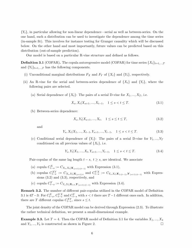
Definition 2.1 (Regular vine). A regular vine (R-vine) on d variables is a sequence of linked
trees (connected acyclic graphs) T1, ..., Td−1 with nodes Ni and edges Ei for i = 1, ..., d−1 which
satisfy the following three conditions.
3
X1 X2 X3 X4 X5
X1, X2 X2, X3 X3, X4 X4, X5
X1, X2 X2, X3 X3, X4 X4, X5
X1, X3|X2 X2, X4|X3 X3, X5|X4
X1, X3|X2 X2, X4|X3 X3, X5|X4
X1, X4|X2:3 X2, X5|X3:4
X1, X4|X2:3 X2, X5|X3:4
X1, X5|X2:4
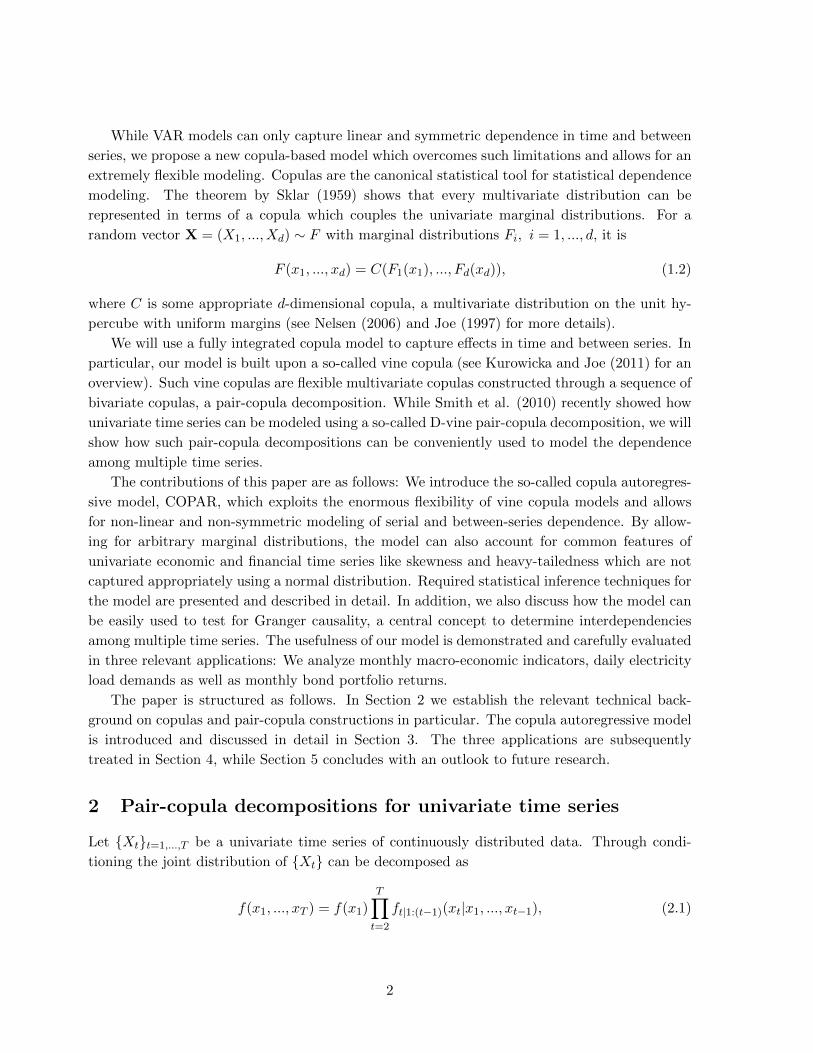
Figure 1: D-vine for T = 5 with edge labels.
(i) Tree T1 has nodes N1 = {1, ..., d}.
(ii) For i = 2, ..., d− 1 tree Ti has nodes Ni = Ei−1.
(iii) If two edges in tree Ti are joined in tree Ti+1, they must share a common node in tree Ti.
The last property is called proximity condition.
D-vines are R-vines, where each node is connected to at most two other nodes. The D-vine
corresponding to the above decomposition is shown in Figure 1.
By associating each edge e = j(e), k(e)|D(e) in an R-vine with a bivariate copula density
cj(e),k(e)|D(e), the complete pair-copula decomposition is defined. The nodes j(e) and k(e) are
called conditioned nodes and D(e) the conditioning set, where in each tree from top to bottom
an additional variable is added in the conditioning set of the bivariate copula.
Theorem 2.2 (R-vine density (Kurowicka and Cooke 2006, Theorem 4.2)). The joint density
of X1, ..., Xd is uniquely determined and given by
f(x1, ..., xd) =
[d∏
k=1
fk(xk)
]×
d−1∏i=1
∏e∈Ei
cj(e),k(e)|D(e)(F (xj(e)|xD(e)), F (xk(e)|xD(e)))
, (2.3)
where xD(e) denotes the sub-vector of x = (x1, ..., xd)′ determined by the indices in D(e).
In (2.3) the arguments of copulas in tree Ti can be recursively computed from copulas in
trees T1, ..., Ti−1 using the general formula
F (x|v) =∂Cxvj |v−j
(F (x|v−j), F (vj |v−j))∂F (vj |v−j)
, (2.4)
where Cxvj |v−jis a bivariate copula, vj is an arbitrary component of v and v−j denotes the
vector v excluding vj .
4
To facilitate statistical inference of R-vines, they can be conveniently stored in matrix no-
tation as recently proposed by Morales-Napoles (2011) and further explored by Dißmann et al.
(2012). Let M ∈ {0, ..., d}d×d be a lower triangular matrix, where the diagonal entries of M
are the numbers 1, ..., d in decreasing order. In this matrix, according to technical conditions,
each row from the bottom up represents a tree, where the conditioned set is identified by a
diagonal entry and by the corresponding column entry of the row under consideration, while the
conditioning set is given by the column entries below this row. Corresponding copula types and
parameters can conveniently be stored in matrices related to M . The fixed ordering of diagonal
entries ensures uniqueness of the R-vine matrix.
The serial D-vine decomposition presented above can be stored in the following matrix
XT
X1 XT−1
X2 X1. . .
......
. . .. . .
......
. . . X3
XT−2 XT−3 · · · · · · X1 X2
XT−1 XT−2 · · · · · · X2 X1 X1
,
which is easily extendible to include future observations {XT+1, XT+2, ...}. For example, the
second entry in the first column identifies the conditioned pair X1 and XT given {X2, ..., XT−1}.Corresponding copula types are stored in the off-diagonal entry associated with the pair:
C1,T |2:(T−1)C2,T |3:(T−1) C1,T−1|2:(T−2)
......
. . ....
.... . .
CT−2,T |T−1 CT−3,T−1|T−2 · · · · · · C1,3|2CT−1,T CT−2,T−1 · · · · · · C2,3 C1,2
.
Here in each row the same copula type must be used. For deriving the joint likelihood the
pair-copulas have to be evaluated in conjunction with the conditional distribution functions.
Using this matrix notation Dißmann et al. (2012) give algorithms to compute the log-
likelihood of an R-vine and to sample from an R-vine. Thus maximum likelihood estimation
of copula parameters is feasible. Copula types are often selected sequentially starting from the
first tree (see also Brechmann et al. (2012)).
3 The copula autoregressive model
Let {Xt}t=1,...,T and {Yt}t=1,...,T be two univariate time series jointly observed at time point
t = 1, ..., T . The aim of this paper is to derive a flexible multivariate distribution of {Xt} and
5
{Yt}, in particular allowing for non-linear dependence—serial as well as between-series. On the
one hand, such a distribution can be used to investigate the dependence among the time series
(in-sample fit). This involves for instance testing for Granger causality which will be discussed
below. On the other hand and most importantly, future values can be predicted based on this
distribution (out-of-sample prediction).
Our model is based on a particular R-vine structure and defined as follows.
Definition 3.1 (COPAR). The copula autoregressive model (COPAR) for time series {Xt}t=1,...,T
and {Yt}t=1,...,T has the following components.
(i) Unconditional marginal distributions FX and FY of {Xt} and {Yt}, respectively.
(ii) An R-vine for the serial and between-series dependence of {Xt} and {Yt}, where the
following pairs are selected.
(a) Serial dependence of {Xt}: The pairs of a serial D-vine for X1, ..., XT , i.e.
Xs, Xt|Xs+1, ..., Xt−1, 1 ≤ s < t ≤ T. (3.1)
(b) Between-series dependence:
Xs, Yt|Xs+1, ..., Xt, 1 ≤ s ≤ t ≤ T, (3.2)
and
Ys, Xt|X1, ..., Xt−1, Ys+1, ..., Yt−1, 1 ≤ s < t ≤ T. (3.3)
(c) Conditional serial dependence of {Yt}: The pairs of a serial D-vine for Y1, ..., YTconditioned on all previous values of {Xt}, i.e.
Ys, Yt|X1, ..., Xt, Ys+1, ..., Yt−1, 1 ≤ s < t ≤ T. (3.4)
Pair-copulas of the same lag length t− s, t ≥ s, are identical. We associate
(a) copula CXt−s := CXs,Xt|X(s+1):(t−1)with Expression (3.1),
(b) copulas CXYt−s := CXs,Yt|X(s+1):tand CY Xt−s := CYs,Xt|X1:(t−1),Y (s+1):(t−1)
with Expres-
sions (3.2) and (3.3), respectively, and
(c) copula CYt−s := CYs,Yt|X1:t,Y (s+1):(t−1)with Expression (3.4).
Remark 3.2. The number of different pair-copulas utilized in the COPAR model of Definition
3.1 is 4T−3: For CXt−s, CY Xt−s and CYt−s with s < t there are T−1 different ones each. In addition,
there are T different copulas CXYt−s , since s ≤ t.
The joint density of the COPAR model can be derived through Expression (2.3). To illustrate
the rather technical definition, we present a small-dimensional example.
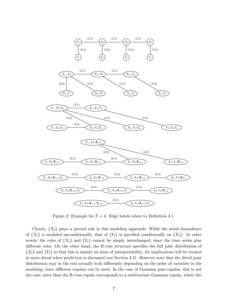
Example 3.3. Let T = 4. Then the COPAR model of Definition 3.1 for the variables X1, ..., X4
and Y1, ..., Y4 is constructed as shown in Figure 2. �
6
X1 X2 X3 X4
Y1 Y2 Y3 Y4
(3.1) (3.1) (3.1)
(3.2) (3.2) (3.2) (3.2)
X1, X2 X2, X3 X3, X4
X1, Y1 X2, Y2 X3, Y3 X4, Y4
(3.1) (3.1)
(3.3) (3.2) (3.2) (3.2)
X1, X3|X2 X2, X4|X3
Y1, X2|X1 X1, Y2|X2 X2, Y3|X3 X3, Y4|X4
(3.1)
(3.3) (3.2) (3.2)
(3.4)
X1, X4|X2:3
Y1, Y2|X1:2 Y2, X3|X1:2 X1, Y3|X2:3 X2, Y4|X3:4
(3.3) (3.2)
(3.3) (3.4)
Y1, X3|X1:2, Y2 Y2, Y3|X1:3 Y3, X4|X1:3 X1, Y4|X2:4
(3.4) (3.3) (3.4)
Y1, Y3|X1:3, Y2 Y2, X4|X1:3, Y3 Y3, Y4|X1:4
(3.3) (3.4)
Y1, X4|X1:3,Y 2:3 Y2, Y4|X1:4, Y3
(3.4)
Figure 2: Example for T = 4. Edge labels relate to Definition 3.1.
Clearly, {Xt} plays a pivotal role in this modeling approach: While the serial dependence
of {Xt} is modeled unconditionally, that of {Yt} is specified conditionally on {Xt}. In other
words, the roles of {Xt} and {Yt} cannot be simply interchanged, since the time series play
different roles. On the other hand, the R-vine structure specifies the full joint distribution of
{Xt} and {Yt} so that this is mainly an issue of interpretability. Its implications will be treated
in more detail when prediction is discussed (see Section 3.3). However note that the fitted joint
distribution may in the end actually look differently depending on the order of variables in the
modeling, since different copulas can be used. In the case of Gaussian pair-copulas, this is not
the case, since then the R-vine copula corresponds to a multivariate Gaussian copula, where the
7
correlation matrix can be computed from conditional correlations as given by the R-vine copula
parameters.
While the serial dependence is rather straightforward to understand from this model, the
modeling of the between-series dependence warrants a more detailed examination. For this
purpose it is useful to look at the R-vine matrices associated to the R-vine structure of Definition
3.1. Here, we continue with Example 3.3 first.
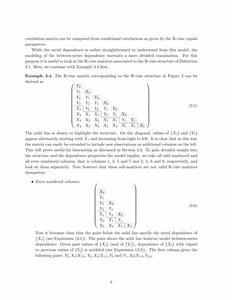
Example 3.4. The R-vine matrix corresponding to the R-vine structure in Figure 2 can be
derived as
Y4Y1 X4
Y2 Y1 Y3Y3 Y2 Y1 X3
X1 Y3 Y2 Y1 Y2X2 X1 X1 Y2 Y1 X2
X3 X2 X2 X1 X1 Y1 Y1X4 X3 X3 X2 X2 X1 X1 X1
. (3.5)
The solid line is drawn to highlight the structure. On the diagonal, values of {Xt} and {Yt}appear alternately starting with X1 and increasing from right to left. It is clear that in this way
the matrix can easily be extended to include new observations as additional columns on the left.
This will prove useful for forecasting as discussed in Section 3.3. To gain detailed insight into
the structure and the dependence properties the model implies, we take all odd numbered and
all even numbered columns, that is columns 1, 3, 5 and 7 and 2, 4, 6 and 8, respectively, and
look at them separately. Note however that these sub-matrices are not valid R-vine matrices
themselves.
• Even numbered columns:
X4
Y1Y2 X3
Y3 Y1X1 Y2 X2
X2 X1 Y1X3 X2 X1 X1
. (3.6)
Now it becomes clear that the pairs below the solid line specify the serial dependence of
{Xt} (see Expression (3.1)). The pairs above the solid line however model between-series
dependence: Given past values of {Xt} (and of {Yt}), dependence of {Xt} with regard
to previous values of {Yt} is modeled (see Expression (3.3)). The first column gives the
following pairs: Y3, X4|X1:3, Y2, X4|X1:3, Y3 and Y1, X4|X1:3, Y2:3.
8
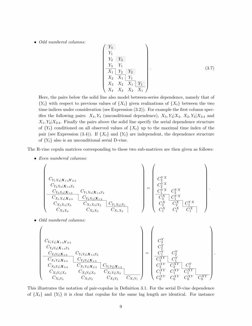
• Odd numbered columns:
Y4Y1Y2 Y3Y3 Y1X1 Y2 Y2X2 X1 Y1X3 X2 X1 Y1X4 X3 X2 X1
. (3.7)
Here, the pairs below the solid line also model between-series dependence, namely that of
{Yt} with respect to previous values of {Xt} given realizations of {Xt} between the two
time indices under consideration (see Expression (3.2)). For example the first column spec-
ifies the following pairs: X4, Y4 (unconditional dependence), X3, Y4|X4, X2, Y4|X3:4 and
X1, Y4|X2:4. Finally the pairs above the solid line specify the serial dependence structure
of {Yt} conditioned on all observed values of {Xt} up to the maximal time index of the
pair (see Expression (3.4)). If {Xt} and {Yt} are independent, the dependence structure
of {Yt} also is an unconditional serial D-vine.
The R-vine copula matrices corresponding to these two sub-matrices are then given as follows:
• Even numbered columns:
CY1X4|X1:3Y 2:3
CY2X4|X1:3Y3
CY3X4|X1:3CY1X3|X1:2Y2
CX1X4|X2:3CY2X3|X1:2
CX2X4|X3CX1X3|X2
CY1X2|X1
CX3X4 CX2X3 CX1X2
=
CY X3
CY X2
CY X1 CY X2
CX3 CY X1
CX2 CX2 CY X1
CX1 CX1 CX1
.
• Odd numbered columns:
CY1Y4|X1:4Y 2:3
CY2Y4|X1:4Y3
CY3Y4|X1:4CY1Y3|X1:3Y2
CX1Y4|X2:4CY2Y3|X1:3
CX2Y4|X3:4CX1Y3|X2:3
CY1Y2|X1:2
CX3Y4|X4CX2Y3|X3
CX1Y2|X2
CX4Y4 CX3Y3 CX2Y2 CX1Y1
=
CY3CY2CY1 CY2CXY3 CY1CXY2 CXY2 CY1CXY1 CXY1 CXY1
CXY0 CXY0 CXY0 CXY0
.
This illustrates the notation of pair-copulas in Definition 3.1. For the serial D-vine dependence
of {Xt} and {Yt} it is clear that copulas for the same lag length are identical. For instance
9
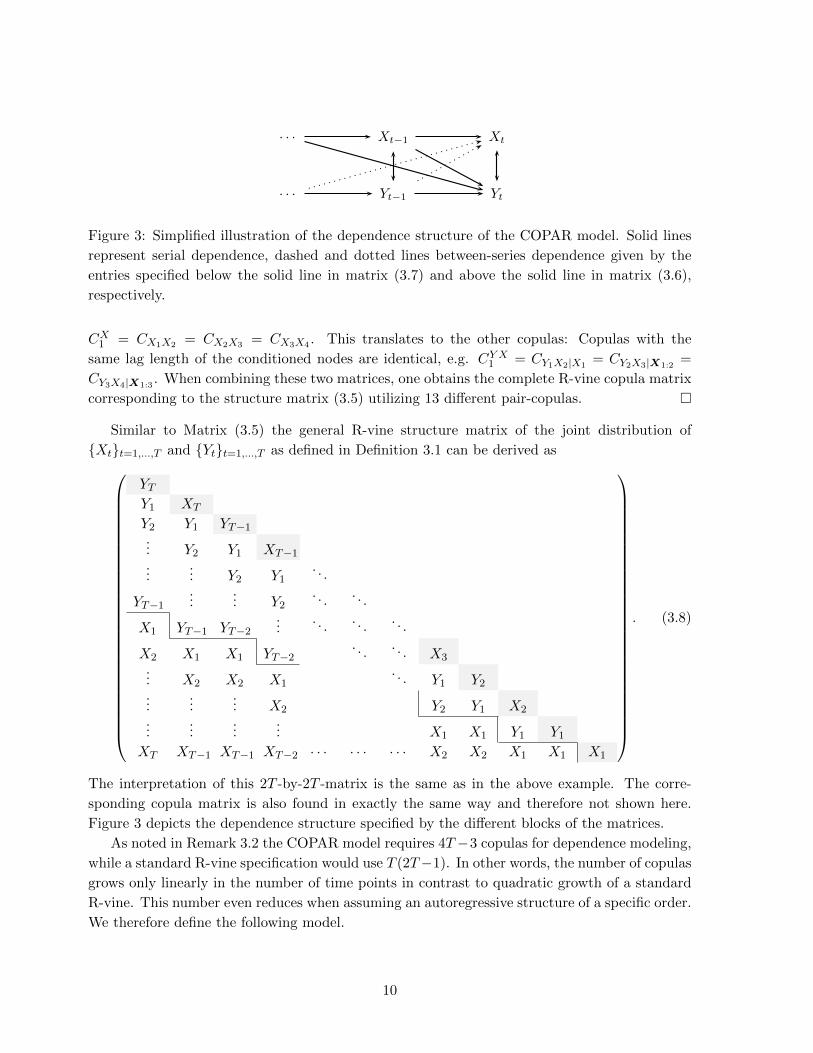
· · · Xt−1 Xt
· · · Yt−1 Yt
Figure 3: Simplified illustration of the dependence structure of the COPAR model. Solid lines
represent serial dependence, dashed and dotted lines between-series dependence given by the
entries specified below the solid line in matrix (3.7) and above the solid line in matrix (3.6),
respectively.
CX1 = CX1X2 = CX2X3 = CX3X4 . This translates to the other copulas: Copulas with the
same lag length of the conditioned nodes are identical, e.g. CY X1 = CY1X2|X1= CY2X3|X1:2
=
CY3X4|X1:3. When combining these two matrices, one obtains the complete R-vine copula matrix
corresponding to the structure matrix (3.5) utilizing 13 different pair-copulas. �
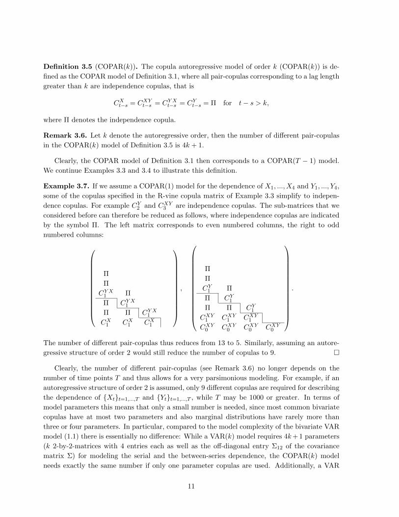
Similar to Matrix (3.5) the general R-vine structure matrix of the joint distribution of
{Xt}t=1,...,T and {Yt}t=1,...,T as defined in Definition 3.1 can be derived as
YTY1 XT
Y2 Y1 YT−1... Y2 Y1 XT−1...
... Y2 Y1. . .
YT−1...
... Y2. . .
. . .
X1 YT−1 YT−2...
. . .. . .
. . .
X2 X1 X1 YT−2. . .
. . . X3
... X2 X2 X1. . . Y1 Y2
......
... X2 Y2 Y1 X2
......
...... X1 X1 Y1 Y1
XT XT−1 XT−1 XT−2 · · · · · · · · · X2 X2 X1 X1 X1
. (3.8)
The interpretation of this 2T -by-2T -matrix is the same as in the above example. The corre-
sponding copula matrix is also found in exactly the same way and therefore not shown here.
Figure 3 depicts the dependence structure specified by the different blocks of the matrices.
As noted in Remark 3.2 the COPAR model requires 4T−3 copulas for dependence modeling,
while a standard R-vine specification would use T (2T−1). In other words, the number of copulas
grows only linearly in the number of time points in contrast to quadratic growth of a standard
R-vine. This number even reduces when assuming an autoregressive structure of a specific order.
We therefore define the following model.
10
Definition 3.5 (COPAR(k)). The copula autoregressive model of order k (COPAR(k)) is de-
fined as the COPAR model of Definition 3.1, where all pair-copulas corresponding to a lag length
greater than k are independence copulas, that is
CXt−s = CXYt−s = CY Xt−s = CYt−s = Π for t− s > k,
where Π denotes the independence copula.
Remark 3.6. Let k denote the autoregressive order, then the number of different pair-copulas
in the COPAR(k) model of Definition 3.5 is 4k + 1.
Clearly, the COPAR model of Definition 3.1 then corresponds to a COPAR(T − 1) model.
We continue Examples 3.3 and 3.4 to illustrate this definition.
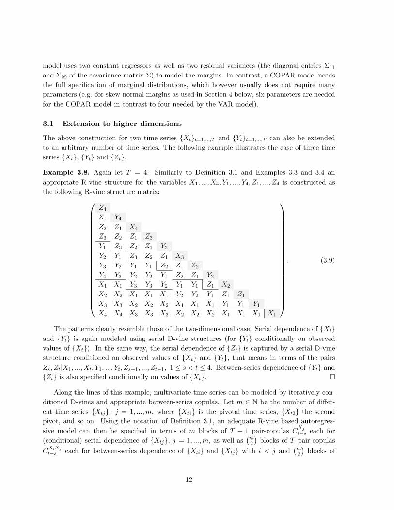
Example 3.7. If we assume a COPAR(1) model for the dependence of X1, ..., X4 and Y1, ..., Y4,
some of the copulas specified in the R-vine copula matrix of Example 3.3 simplify to indepen-
dence copulas. For example CY2 and CXY3 are independence copulas. The sub-matrices that we
considered before can therefore be reduced as follows, where independence copulas are indicated
by the symbol Π. The left matrix corresponds to even numbered columns, the right to odd
numbered columns:
Π
Π
CY X1 Π
Π CY X1
Π Π CY X1
CX1 CX1 CX1
,
Π
Π
CY1 Π
Π CY1Π Π CY1
CXY1 CXY1 CXY1
CXY0 CXY0 CXY0 CXY0
.
The number of different pair-copulas thus reduces from 13 to 5. Similarly, assuming an autore-
gressive structure of order 2 would still reduce the number of copulas to 9. �
Clearly, the number of different pair-copulas (see Remark 3.6) no longer depends on the
number of time points T and thus allows for a very parsimonious modeling. For example, if an
autoregressive structure of order 2 is assumed, only 9 different copulas are required for describing
the dependence of {Xt}t=1,...,T and {Yt}t=1,...,T , while T may be 1000 or greater. In terms of
model parameters this means that only a small number is needed, since most common bivariate
copulas have at most two parameters and also marginal distributions have rarely more than
three or four parameters. In particular, compared to the model complexity of the bivariate VAR
model (1.1) there is essentially no difference: While a VAR(k) model requires 4k+ 1 parameters
(k 2-by-2-matrices with 4 entries each as well as the off-diagonal entry Σ12 of the covariance
matrix Σ) for modeling the serial and the between-series dependence, the COPAR(k) model
needs exactly the same number if only one parameter copulas are used. Additionally, a VAR
11
model uses two constant regressors as well as two residual variances (the diagonal entries Σ11
and Σ22 of the covariance matrix Σ) to model the margins. In contrast, a COPAR model needs
the full specification of marginal distributions, which however usually does not require many
parameters (e.g. for skew-normal margins as used in Section 4 below, six parameters are needed
for the COPAR model in contrast to four needed by the VAR model).
3.1 Extension to higher dimensions
The above construction for two time series {Xt}t=1,...,T and {Yt}t=1,...,T can also be extended
to an arbitrary number of time series. The following example illustrates the case of three time
series {Xt}, {Yt} and {Zt}.
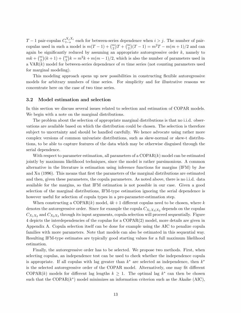
Example 3.8. Again let T = 4. Similarly to Definition 3.1 and Examples 3.3 and 3.4 an
appropriate R-vine structure for the variables X1, ..., X4, Y1, ..., Y4, Z1, ..., Z4 is constructed as
the following R-vine structure matrix:
Z4
Z1 Y4Z2 Z1 X4
Z3 Z2 Z1 Z3
Y1 Z3 Z2 Z1 Y3Y2 Y1 Z3 Z2 Z1 X3
Y3 Y2 Y1 Y1 Z2 Z1 Z2
Y4 Y3 Y2 Y2 Y1 Z2 Z1 Y2X1 X1 Y3 Y3 Y2 Y1 Y1 Z1 X2
X2 X2 X1 X1 X1 Y2 Y2 Y1 Z1 Z1
X3 X3 X2 X2 X2 X1 X1 X1 Y1 Y1 Y1X4 X4 X3 X3 X3 X2 X2 X2 X1 X1 X1 X1
. (3.9)
The patterns clearly resemble those of the two-dimensional case. Serial dependence of {Xt}and {Yt} is again modeled using serial D-vine structures (for {Yt} conditionally on observed
values of {Xt}). In the same way, the serial dependence of {Zt} is captured by a serial D-vine
structure conditioned on observed values of {Xt} and {Yt}, that means in terms of the pairs
Zs, Zt|X1, ..., Xt, Y1, ..., Yt, Zs+1, ..., Zt−1, 1 ≤ s < t ≤ 4. Between-series dependence of {Yt} and
{Zt} is also specified conditionally on values of {Xt}. �
Along the lines of this example, multivariate time series can be modeled by iteratively con-
ditioned D-vines and appropriate between-series copulas. Let m ∈ N be the number of differ-
ent time series {Xtj}, j = 1, ...,m, where {Xt1} is the pivotal time series, {Xt2} the second
pivot, and so on. Using the notation of Definition 3.1, an adequate R-vine based autoregres-
sive model can then be specified in terms of m blocks of T − 1 pair-copulas CXj
t−s each for
(conditional) serial dependence of {Xtj}, j = 1, ...,m, as well as(m2
)blocks of T pair-copulas
CXiXj
t−s each for between-series dependence of {Xti} and {Xtj} with i < j and(m2
)blocks of
12
T − 1 pair-copulas CXjXi
t−s each for between-series dependence when i > j. The number of pair-
copulas used in such a model is m(T − 1) +(m2
)T +
(m2
)(T − 1) = m2T −m(m+ 1)/2 and can
again be significantly reduced by assuming an appropriate autoregressive order k, namely to
mk +(m2
)(k + 1) +
(m2
)k = m2k +m(m− 1)/2, which is also the number of parameters used in
a VAR(k) model for between-series dependence of m time series (not counting parameters used
for marginal modeling).
This modeling approach opens up new possibilities in constructing flexible autoregressive
models for arbitrary numbers of time series. For simplicity and for illustrative reasons we
concentrate here on the case of two time series.
3.2 Model estimation and selection
In this section we discuss several issues related to selection and estimation of COPAR models.
We begin with a note on the marginal distributions.
The problem about the selection of appropriate marginal distributions is that no i.i.d. obser-
vations are available based on which the distribution could be chosen. The selection is therefore
subject to uncertainty and should be handled carefully. We hence advocate using rather more
complex versions of common univariate distributions, such as skew-normal or skew-t distribu-
tions, to be able to capture features of the data which may be otherwise disguised through the
serial dependence.
With respect to parameter estimation, all parameters of a COPAR(k) model can be estimated
jointly by maximum likelihood techniques, since the model is rather parsimonious. A common
alternative in the literature is estimation using inference functions for margins (IFM) by Joe
and Xu (1996). This means that first the parameters of the marginal distributions are estimated
and then, given these parameters, the copula parameters. As noted above, there is no i.i.d. data
available for the margins, so that IFM estimation is not possible in our case. Given a good
selection of the marginal distributions, IFM-type estimation ignoring the serial dependence is
however useful for selection of copula types in a pre-parameter-estimation step.
When constructing a COPAR(k) model, 4k+ 1 different copulas need to be chosen, where k
denotes the autoregressive order. Since for example the copula CX1X3|X2depends on the copulas
CX1X2 and CX2X3 through its input arguments, copula selection will proceed sequentially. Figure
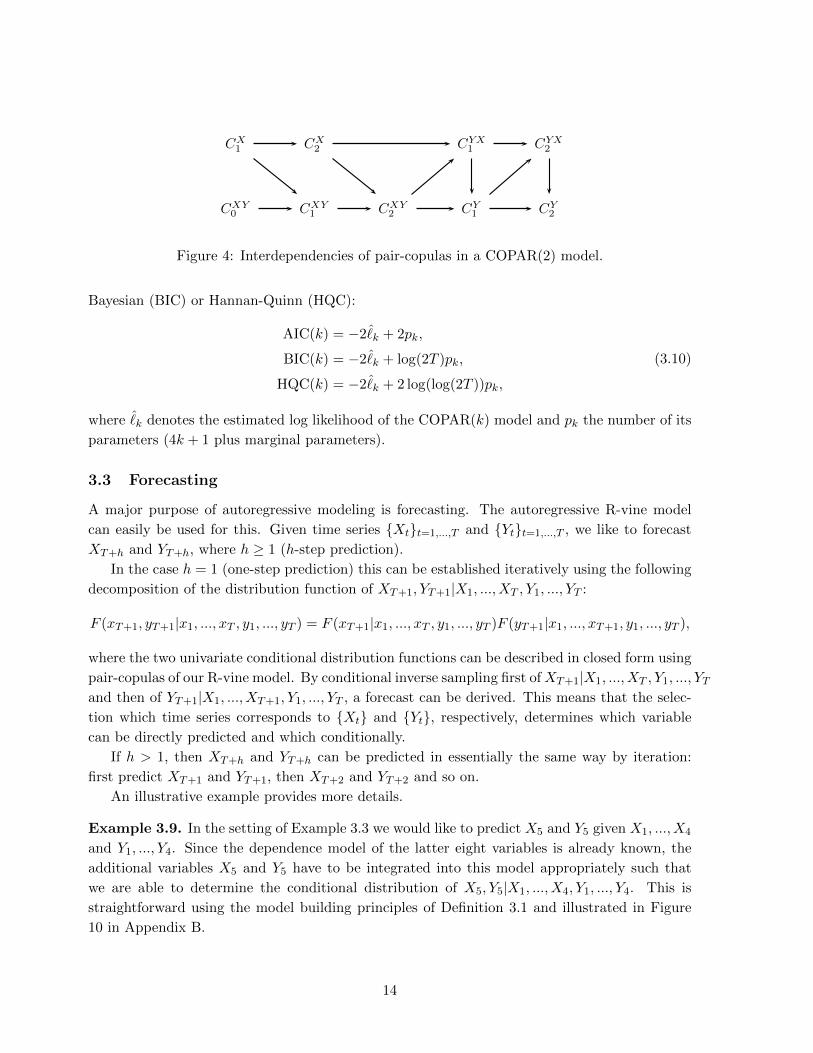
4 depicts the interdependencies of the copulas for a COPAR(2) model, more details are given in
Appendix A. Copula selection itself can be done for example using the AIC to penalize copula
families with more parameters. Note that models can also be estimated in this sequential way.
Resulting IFM-type estimates are typically good starting values for a full maximum likelihood
estimation.
Finally, the autoregressive order has to be selected. We propose two methods. First, when
selecting copulas, an independence test can be used to check whether the independence copula
is appropriate. If all copulas with lag greater than k∗ are selected as independence, then k∗
is the selected autoregressive order of the COPAR model. Alternatively, one may fit different
COPAR(k) models for different lag lengths k ≥ 1. The optimal lag k∗ can then be chosen
such that the COPAR(k∗) model minimizes an information criterion such as the Akaike (AIC),
13
CX1 CX
2 CYX1 CYX
2
CXY0 CXY
1 CXY2 CY
1 CY2
Figure 4: Interdependencies of pair-copulas in a COPAR(2) model.
Bayesian (BIC) or Hannan-Quinn (HQC):
AIC(k) = −2ˆk + 2pk,
BIC(k) = −2ˆk + log(2T )pk,
HQC(k) = −2ˆk + 2 log(log(2T ))pk,
(3.10)
where ˆk denotes the estimated log likelihood of the COPAR(k) model and pk the number of its
parameters (4k + 1 plus marginal parameters).
3.3 Forecasting
A major purpose of autoregressive modeling is forecasting. The autoregressive R-vine model
can easily be used for this. Given time series {Xt}t=1,...,T and {Yt}t=1,...,T , we like to forecast
XT+h and YT+h, where h ≥ 1 (h-step prediction).
In the case h = 1 (one-step prediction) this can be established iteratively using the following
decomposition of the distribution function of XT+1, YT+1|X1, ..., XT , Y1, ..., YT :
F (xT+1, yT+1|x1, ..., xT , y1, ..., yT ) = F (xT+1|x1, ..., xT , y1, ..., yT )F (yT+1|x1, ..., xT+1, y1, ..., yT ),
where the two univariate conditional distribution functions can be described in closed form using
pair-copulas of our R-vine model. By conditional inverse sampling first ofXT+1|X1, ..., XT , Y1, ..., YTand then of YT+1|X1, ..., XT+1, Y1, ..., YT , a forecast can be derived. This means that the selec-
tion which time series corresponds to {Xt} and {Yt}, respectively, determines which variable
can be directly predicted and which conditionally.
If h > 1, then XT+h and YT+h can be predicted in essentially the same way by iteration:
first predict XT+1 and YT+1, then XT+2 and YT+2 and so on.
An illustrative example provides more details.
Example 3.9. In the setting of Example 3.3 we would like to predict X5 and Y5 given X1, ..., X4
and Y1, ..., Y4. Since the dependence model of the latter eight variables is already known, the
additional variables X5 and Y5 have to be integrated into this model appropriately such that
we are able to determine the conditional distribution of X5, Y5|X1, ..., X4, Y1, ..., Y4. This is
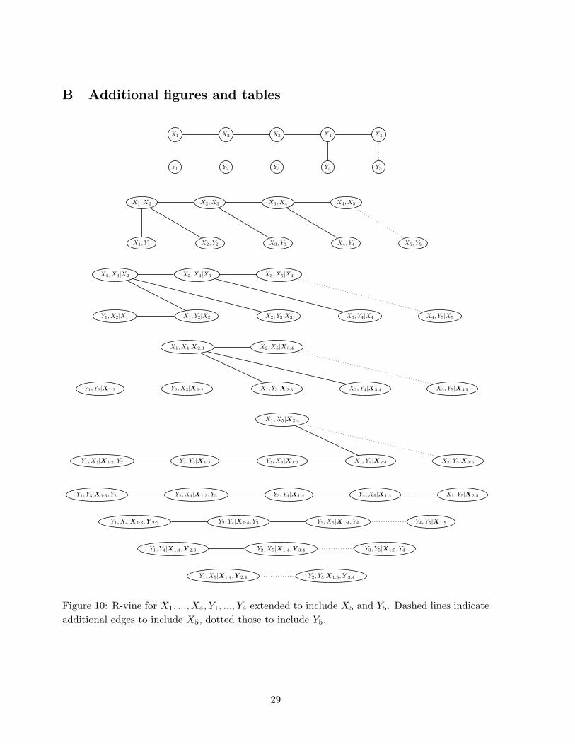
straightforward using the model building principles of Definition 3.1 and illustrated in Figure
10 in Appendix B.
14
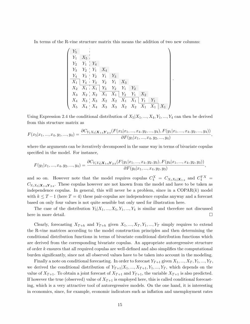
In terms of the R-vine structure matrix this means the addition of two new columns:
Y5Y1 X5
Y2 Y1 Y4Y3 Y2 Y1 X4
Y4 Y3 Y2 Y1 Y3X1 Y4 Y3 Y2 Y1 X3
X2 X1 X1 Y3 Y2 Y1 Y2X3 X2 X2 X1 X1 Y2 Y1 X2
X4 X3 X3 X2 X2 X1 X1 Y1 Y1X5 X4 X4 X3 X3 X2 X2 X1 X1 X1
.
Using Expression 2.4 the conditional distribution of X5|X1, ..., X4, Y1, ..., Y4 can then be derived
from this structure matrix as
F (x5|x1, ..., x4, y1, ..., y4) =∂CY1X5|X1:4Y 2:4
(F (x5|x1, ..., x4, y2, ..., y4), F (y1|x1, ..., x4, y2, ..., y4))∂F (y1|x1, ..., x4, y2, ..., y4)
,
where the arguments can be iteratively decomposed in the same way in terms of bivariate copulas
specified in the model. For instance,
F (y1|x1, ..., x4, y2, ..., y4) =∂CY1Y4|X1:4Y 2:3
(F (y1|x1, ..., x4, y2, y3), F (y4|x1, ..., x4, y2, y3))∂F (y4|x1, ..., x4, y2, y3)
,
and so on. However note that the model requires copulas CX4 = CX1X5|X1:4and CY X4 =
CY1X5|X1:4Y 2:4. These copulas however are not known from the model and have to be taken as
independence copulas. In general, this will never be a problem, since in a COPAR(k) model
with k ≤ T − 1 (here T = 4) these pair-copulas are independence copulas anyway and a forecast
based on only four values is not quite sensible but only used for illustration here.
The case of the distribution Y5|X1, ..., X5, Y1, ..., Y4 is similar and therefore not discussed
here in more detail. �
Clearly, forecasting XT+h and YT+h given X1, ..., XT , Y1, ..., YT simply requires to extend
the R-vine matrices according to the model construction principles and then determining the
conditional distribution functions in terms of bivariate conditional distribution functions which
are derived from the corresponding bivariate copulas. An appropriate autoregressive structure
of order k ensures that all required copulas are well-defined and also simplifies the computational
burden significantly, since not all observed values have to be taken into account in the modeling.
Finally a note on conditional forecasting. In order to forecast YT+1 givenX1, ..., XT , Y1, ..., YT ,
we derived the conditional distribution of YT+1|X1, ..., XT+1, Y1, ..., YT , which depends on the
value of XT+1. To obtain a joint forecast of XT+1 and YT+1, the variable XT+1 is also predicted.
If however the true (observed) value of XT+1 is employed here, this is called conditional forecast-
ing, which is a very attractive tool of autoregressive models. On the one hand, it is interesting
in economics, since, for example, economic indicators such as inflation and unemployment rates
15
are often not released simultaneously. Let us assume that inflation rates are released first. This
information could then be used to obtain more accurate forecasts of unemployment rates. Ad-
ditionally, conditional forecasting is very useful for scenario analysis, for instance to investigate
the impact of shocks to markets.
3.4 Granger causality
Granger causality of a time series {Yt}t=1,...,T with respect to another time series {Xt}t=1,...,T
means that {Yt} provides statistically significant information about {Xt}, in other words, it is
helpful to predict {Xt}. This is often denoted as {Yt} → {Xt} (“{Yt} Granger causes {Xt}.”).
On the other hand, {Yt}t=1,...,T does not Granger cause {Xt}t=1,...,T if it does not have any
explanatory power with respect to future observations XT+s, s ≥ 1.
Granger causality of one time series on another can easily be investigated using the COPAR
model. As discussed above, the COPAR model directly gives the conditional distribution of
XT+1|X1, ..., XT , Y1, ..., YT . If {Yt} does not Granger cause {Xt}, then this distribution is equal
to that of XT+1|X1, ..., XT , which means that all the pairs specifying between-series dependence
of {Xt} and {Yt} (see Expressions (3.2) and (3.3)) are independent. The model then collapses
to two independent serial D-vines for {Xt} and {Yt}, respectively. When pair-copulas of these
two serial D-vines are chosen as for the pairs in the full model, then the two models are nested
(most copulas, in particular those that will be considered in this paper, include the independence
copula as special or boundary case) and a standard likelihood-ratio test can be used to investigate
Granger causality. Let `RV denote the log likelihood of the joint model of {Xt} and {Yt} and
`DV the cumulative one of the two separate D-vines for {Xt} and {Yt} constructed with the
same pair-copulas as the joint model, then
2(`RV − `DV )as.∼ χ2
pRV −pDV, (3.11)
where χ2q denotes a χ2 distribution with q degrees of freedom and pRV and pDV denote the
number of parameters of the full (R-vine) and the reduced (two D-vines) model, respectively.
If copula families are however chosen differently, then a test for non-nested hypotheses such as
the one by Vuong (1989) can be used.
To summarize, in order to investigate Granger causality of a time series {Yt}t=1,...,T on
another time series {Xt}t=1,...,T , the COPAR model can be used in conjunction with a likelihood-
ratio test. If Granger causality of {Xt} on {Yt} is to be investigated, the roles of the two time
series have to be interchanged.
4 Applications
In this section we discuss three relevant applications. First, we analyze four monthly macro-
economic indicators pairwisely, namely inflation and interest rates as well as stock returns and
industrial production. Since this is the classical area of application of VAR models it is partic-
ularly interesting to see what COPAR models can add here. Second, COPAR models are used
to model daily electricity load demands in four Australian states. Due to geography there is a
16
strong interdependence among states which needs to be captured. Finally, monthly Fama bond
portfolio returns with medium duration are analyzed.
In each of the three data sets we compare the COPAR model to relevant benchmark mod-
els in terms of out-of-sample predictive ability: First, VAR(k) models are fitted using the
R-package vars (Pfaff 2008). Second, we also fit standard copula models with AR(k) and
AR(k)-GARCH(1,1) margins, where the distribution of the innovations is chosen as in the
corresponding COPAR model and the copula used is selected according to the AIC from a
range of different copulas capturing all types of dependence (tail-independent Gaussian (N) and
Frank (F), symmetric-tail-dependent Student-t, lower-tail-dependent Clayton (C), upper-tail-
dependent Gumbel (G) and Joe (J), and their survival versions (SC, SG, SJ)). Note that the
copula model with AR(k)-GARCH(1,1) is a very tough competitor model, since it allows for
time-varying variances, which the COPAR and the VAR models do not. Since the use of copula-
GARCH models is a common tool for the analysis of financial time series, it is also included in
the analysis.
For COPAR models we distinguish
• unconditional prediction of XT+1 given X1, ..., XT , Y1, ..., YT ,
• joint prediction of XT+1 and YT+1 given X1, ..., XT , Y1, ..., YT , and
• conditional prediction of YT+1 given X1, ..., XT+1, Y1, ..., YT .
To speed up computations IFM-type sequential estimation as described in Section 3.2 is used
for out-of-sample prediction, since the model is re-estimated for each additional prediction. In
all three applications model parameters estimated in this way were very close to full maximum
likelihood estimates. Copulas are selected as described in Section 3.2 and from the same list as
above.
Predictions are evaluated in terms of two different loss functions. On the one hand, we
consider the classical root mean squared error
RMSE(x;x) =
√√√√ 1
T ∗
T ∗∑t=1
(xi − xi)2,
where T ∗ denotes the number of out-of-sample predictions and x = (x1, ..., xT ∗)′ are point
forecasts of x = (x1, ..., xT ∗)′. On the other hand, in order to check the coverage of empirical
prediction intervals, mean interval scores by Gneiting and Raftery (2007) are taken into account:
MISα(l, u;x) =1
T ∗
T ∗∑t=1
[(ui − li
)+
2
α
(li − xi
)1{xi<li} +
2
α
(xi − ui
)1{ui<xi}
],
where l = (l1, ..., lT ∗)′ and u = (u1, ..., uT ∗)
′, and [li, ui], i = 1, ..., T ∗, are 100(1−α)% prediction
intervals. For the copula-based models these are determined as (α/2) and (1 − α/2) sample
quantiles; for the VAR model closed form expressions using normal quantiles are used.
17
0 100 200 300 400 500
−0.
100.
000.
10
MKT
0 100 200 300 400 500−0.
006
0.00
00.
004
RRF
0 100 200 300 400 500
−0.
005
0.00
50.
015
INF
0 100 200 300 400 500
−0.
040.
000.
04
IPG
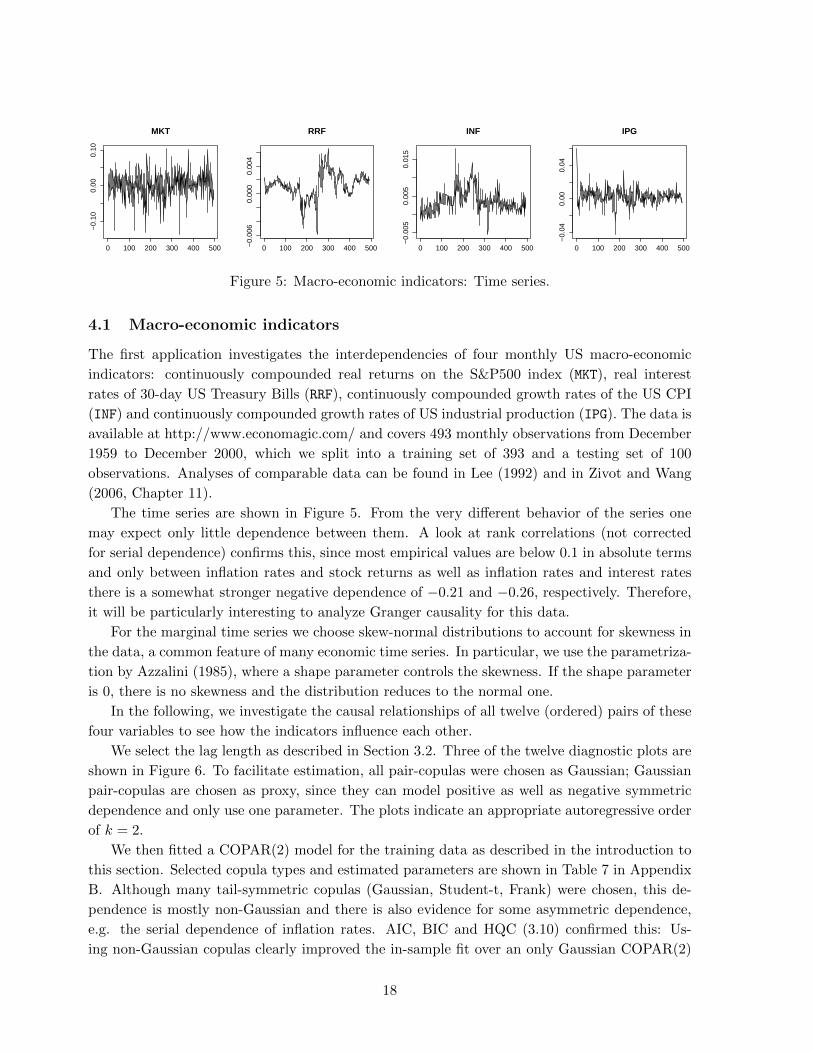
Figure 5: Macro-economic indicators: Time series.
4.1 Macro-economic indicators
The first application investigates the interdependencies of four monthly US macro-economic
indicators: continuously compounded real returns on the S&P500 index (MKT), real interest
rates of 30-day US Treasury Bills (RRF), continuously compounded growth rates of the US CPI
(INF) and continuously compounded growth rates of US industrial production (IPG). The data is
available at http://www.economagic.com/ and covers 493 monthly observations from December
1959 to December 2000, which we split into a training set of 393 and a testing set of 100
observations. Analyses of comparable data can be found in Lee (1992) and in Zivot and Wang
(2006, Chapter 11).
The time series are shown in Figure 5. From the very different behavior of the series one
may expect only little dependence between them. A look at rank correlations (not corrected
for serial dependence) confirms this, since most empirical values are below 0.1 in absolute terms
and only between inflation rates and stock returns as well as inflation rates and interest rates
there is a somewhat stronger negative dependence of −0.21 and −0.26, respectively. Therefore,
it will be particularly interesting to analyze Granger causality for this data.
For the marginal time series we choose skew-normal distributions to account for skewness in
the data, a common feature of many economic time series. In particular, we use the parametriza-
tion by Azzalini (1985), where a shape parameter controls the skewness. If the shape parameter
is 0, there is no skewness and the distribution reduces to the normal one.
In the following, we investigate the causal relationships of all twelve (ordered) pairs of these
four variables to see how the indicators influence each other.
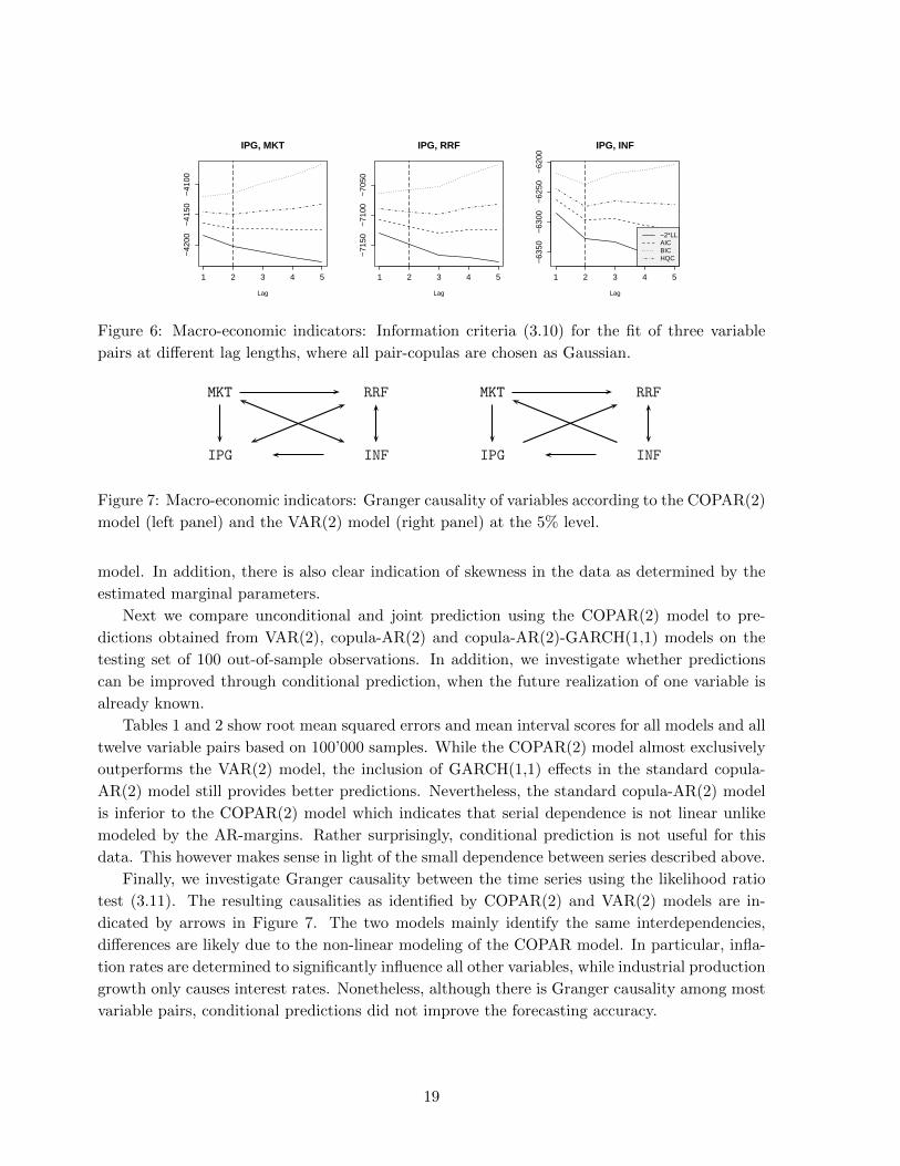
We select the lag length as described in Section 3.2. Three of the twelve diagnostic plots are
shown in Figure 6. To facilitate estimation, all pair-copulas were chosen as Gaussian; Gaussian
pair-copulas are chosen as proxy, since they can model positive as well as negative symmetric
dependence and only use one parameter. The plots indicate an appropriate autoregressive order
of k = 2.
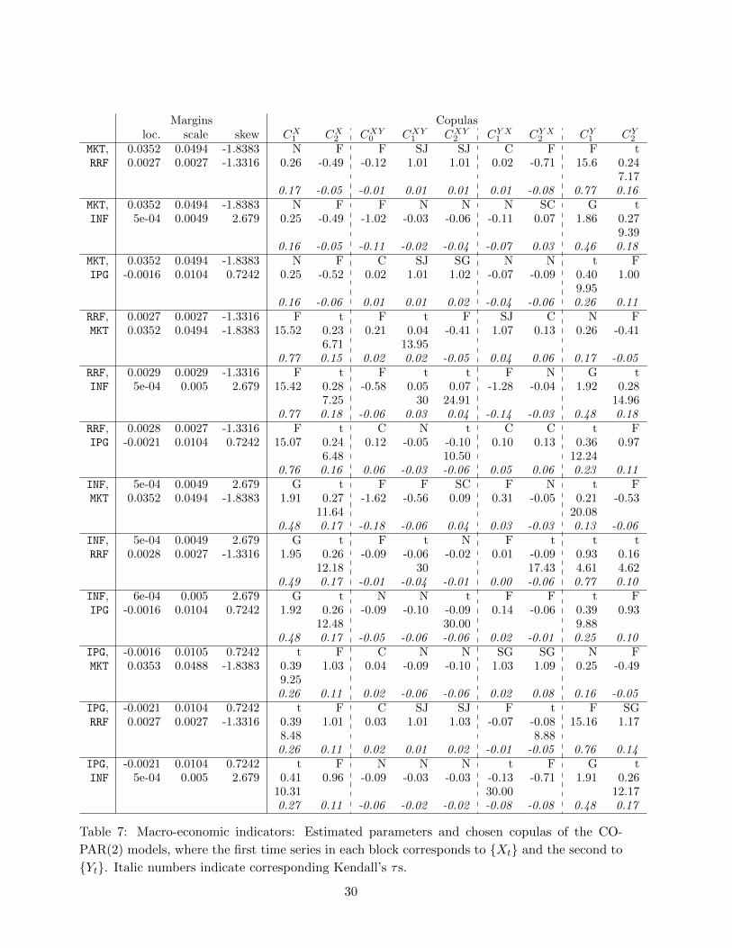
We then fitted a COPAR(2) model for the training data as described in the introduction to
this section. Selected copula types and estimated parameters are shown in Table 7 in Appendix
B. Although many tail-symmetric copulas (Gaussian, Student-t, Frank) were chosen, this de-
pendence is mostly non-Gaussian and there is also evidence for some asymmetric dependence,
e.g. the serial dependence of inflation rates. AIC, BIC and HQC (3.10) confirmed this: Us-
ing non-Gaussian copulas clearly improved the in-sample fit over an only Gaussian COPAR(2)
18
1 2 3 4 5
−42
00−
4150
−41
00
IPG, MKT
Lag
1 2 3 4 5
−71
50−
7100
−70
50
IPG, RRF
Lag
1 2 3 4 5
−63
50−
6300
−62
50−
6200
IPG, INF
Lag
−2*LLAICBICHQC
Figure 6: Macro-economic indicators: Information criteria (3.10) for the fit of three variable
pairs at different lag lengths, where all pair-copulas are chosen as Gaussian.
MKT 00RRF00
0000IPG0000 0000INF0000
MKT 00RRF00
0000IPG0000 0000INF0000
Figure 7: Macro-economic indicators: Granger causality of variables according to the COPAR(2)
model (left panel) and the VAR(2) model (right panel) at the 5% level.
model. In addition, there is also clear indication of skewness in the data as determined by the
estimated marginal parameters.
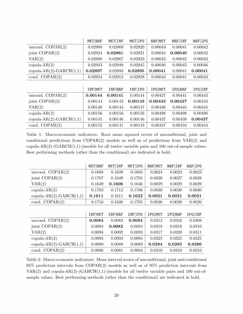
Next we compare unconditional and joint prediction using the COPAR(2) model to pre-
dictions obtained from VAR(2), copula-AR(2) and copula-AR(2)-GARCH(1,1) models on the
testing set of 100 out-of-sample observations. In addition, we investigate whether predictions
can be improved through conditional prediction, when the future realization of one variable is
already known.
Tables 1 and 2 show root mean squared errors and mean interval scores for all models and all
twelve variable pairs based on 100’000 samples. While the COPAR(2) model almost exclusively
outperforms the VAR(2) model, the inclusion of GARCH(1,1) effects in the standard copula-
AR(2) model still provides better predictions. Nevertheless, the standard copula-AR(2) model
is inferior to the COPAR(2) model which indicates that serial dependence is not linear unlike
modeled by the AR-margins. Rather surprisingly, conditional prediction is not useful for this
data. This however makes sense in light of the small dependence between series described above.
Finally, we investigate Granger causality between the time series using the likelihood ratio
test (3.11). The resulting causalities as identified by COPAR(2) and VAR(2) models are in-
dicated by arrows in Figure 7. The two models mainly identify the same interdependencies,
differences are likely due to the non-linear modeling of the COPAR model. In particular, infla-
tion rates are determined to significantly influence all other variables, while industrial production
growth only causes interest rates. Nonetheless, although there is Granger causality among most
variable pairs, conditional predictions did not improve the forecasting accuracy.
19
MKT|RRF MKT|INF MKT|IPG RRF|MKT RRF|INF RRF|IPGuncond. COPAR(2) 0.02908 0.02869 0.02920 0.00043 0.00041 0.00042
joint COPAR(2) 0.02924 0.02861 0.02921 0.00044 0.00040 0.00042
VAR(2) 0.02900 0.02867 0.02923 0.00042 0.00042 0.00043
copula-AR(2) 0.02943 0.02948 0.02945 0.00046 0.00045 0.00046
copula-AR(2)-GARCH(1,1) 0.02897 0.02893 0.02895 0.00041 0.00041 0.00041
cond. COPAR(2) 0.02924 0.02912 0.02928 0.00043 0.00041 0.00043
INF|MKT INF|RRF INF|IPG IPG|MKT IPG|RRF IPG|INFuncond. COPAR(2) 0.00144 0.00141 0.00144 0.00437 0.00441 0.00443
joint COPAR(2) 0.00144 0.00143 0.00143 0.00433 0.00437 0.00443
VAR(2) 0.00148 0.00144 0.00147 0.00446 0.00445 0.00445
copula-AR(2) 0.00156 0.00156 0.00156 0.00498 0.00498 0.00498
copula-AR(2)-GARCH(1,1) 0.00145 0.00146 0.00146 0.00437 0.00438 0.00437
cond. COPAR(2) 0.00152 0.00141 0.00143 0.00437 0.00434 0.00444
Table 1: Macro-economic indicators: Root mean squared errors of unconditional, joint and
conditional predictions from COPAR(2) models as well as of predictions from VAR(2) and
copula-AR(2)-(GARCH(1,1)-)models for all twelve variable pairs and 100 out-of-sample values.
Best performing methods (other than the conditional) are indicated in bold.
MKT|RRF MKT|INF MKT|IPG RRF|MKT RRF|INF RRF|IPGuncond. COPAR(2) 0.1688 0.1639 0.1693 0.0024 0.0023 0.0023
joint COPAR(2) 0.1707 0.1649 0.1705 0.0026 0.0027 0.0028
VAR(2) 0.1649 0.1606 0.1646 0.0029 0.0029 0.0029
copula-AR(2) 0.1703 0.1712 0.1706 0.0030 0.0030 0.0030
copula-AR(2)-GARCH(1,1) 0.1611 0.1611 0.1622 0.0021 0.0021 0.0021
cond. COPAR(2) 0.1716 0.1626 0.1705 0.0026 0.0026 0.0026
INF|MKT INF|RRF INF|IPG IPG|MKT IPG|RRF IPG|INFuncond. COPAR(2) 0.0084 0.0083 0.0084 0.0312 0.0316 0.0308
joint COPAR(2) 0.0084 0.0082 0.0084 0.0318 0.0316 0.0310
VAR(2) 0.0094 0.0092 0.0093 0.0317 0.0320 0.0311
copula-AR(2) 0.0094 0.0093 0.0094 0.0325 0.0325 0.0325
copula-AR(2)-GARCH(1,1) 0.0089 0.0089 0.0089 0.0284 0.0285 0.0286
cond. COPAR(2) 0.0086 0.0081 0.0084 0.0316 0.0310 0.0310
Table 2: Macro-economic indicators: Mean interval scores of unconditional, joint and conditional
95% prediction intervals from COPAR(2) models as well as of 95% prediction intervals from
VAR(2) and copula-AR(2)-(GARCH(1,1)-)models for all twelve variable pairs and 100 out-of-
sample values. Best performing methods (other than the conditional) are indicated in bold.
20
0 200 400 600 800 1000
−3
−2
−1
01
2
QLD
0 200 400 600 800 1000−
3−
2−
10
12
3
NSW
0 200 400 600 800 1000
−3
−2
−1
01
23
VIC
0 200 400 600 800 1000
−3
−2
−1
01
23
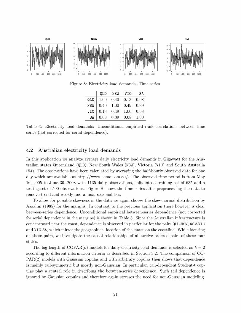
SA
Figure 8: Electricity load demands: Time series.
QLD NSW VIC SA
QLD 1.00 0.40 0.13 0.08
NSW 0.40 1.00 0.49 0.39
VIC 0.13 0.49 1.00 0.68
SA 0.08 0.39 0.68 1.00
Table 3: Electricity load demands: Unconditional empirical rank correlations between time
series (not corrected for serial dependence).
4.2 Australian electricity load demands
In this application we analyze average daily electricity load demands in Gigawatt for the Aus-
tralian states Queensland (QLD), New South Wales (NSW), Victoria (VIC) and South Australia
(SA). The observations have been calculated by averaging the half-hourly observed data for one
day which are available at http://www.aemo.com.au/. The observed time period is from May
16, 2005 to June 30, 2008 with 1135 daily observations, split into a training set of 635 and a
testing set of 500 observations. Figure 8 shows the time series after preprocessing the data to
remove trend and weekly and annual seasonalities.
To allow for possible skewness in the data we again choose the skew-normal distribution by
Azzalini (1985) for the margins. In contrast to the previous application there however is clear
between-series dependence. Unconditional empirical between-series dependence (not corrected
for serial dependence in the margins) is shown in Table 3. Since the Australian infrastructure is
concentrated near the coast, dependence is observed in particular for the pairs QLD-NSW, NSW-VIC
and VIC-SA, which mirror the geographical location of the states on the coastline. While focusing
on these pairs, we investigate the causal relationships of all twelve ordered pairs of these four
states.
The lag length of COPAR(k) models for daily electricity load demands is selected as k = 2
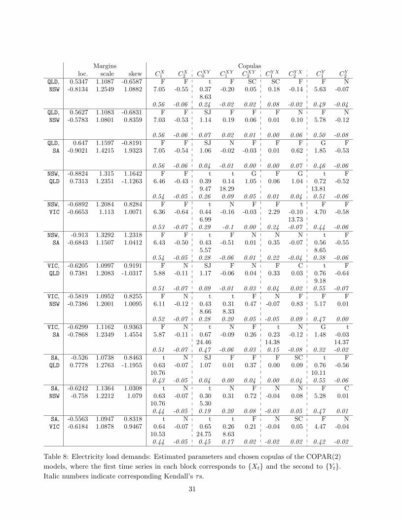
according to different information criteria as described in Section 3.2. The comparison of CO-
PAR(2) models with Gaussian copulas and with arbitrary copulas then shows that dependence
is mainly tail-symmetric but mostly non-Gaussian. In particular, tail-dependent Student-t cop-
ulas play a central role in describing the between-series dependence. Such tail dependence is
ignored by Gaussian copulas and therefore again stresses the need for non-Gaussian modeling.
21
QLD|NSW QLD|VIC QLD|SA NSW|QLD NSW|VIC NSW|SAuncond. COPAR(2) 0.653 0.648 0.645 0.692 0.674 0.679
joint COPAR(2) 0.663 0.670 0.657 0.706 0.674 0.689
VAR(2) 0.674 0.670 0.668 0.697 0.690 0.690
copula-AR(2) 0.673 0.674 0.673 0.697 0.697 0.697
copula-AR(2)-GARCH(1,1) 0.679 0.679 0.679 0.699 0.699 0.698
cond. COPAR(2) 0.606 0.624 0.627 0.654 0.603 0.639
VIC|QLD VIC|NSW VIC|SA SA|QLD SA|NSW SA|VICuncond. COPAR(2) 0.676 0.674 0.666 0.691 0.686 0.691
joint COPAR(2) 0.672 0.679 0.684 0.690 0.686 0.679
VAR(2) 0.693 0.692 0.685 0.687 0.684 0.688
copula-AR(2) 0.690 0.690 0.689 0.686 0.687 0.685
copula-AR(2)-GARCH(1,1) 0.692 0.692 0.692 0.687 0.687 0.687
cond. COPAR(2) 0.638 0.598 0.555 0.666 0.644 0.560
Table 4: Electricity load demands: Root mean squared errors of unconditional, joint and con-
ditional predictions from COPAR(2) models as well as of predictions from VAR(2) and copula-
AR(2)-(GARCH(1,1)-)models for all twelve variable pairs and 500 out-of-sample values. Best
performing methods (other than the conditional) are indicated in bold.
Selected copula types and estimated parameters are shown in Table 8 in Appendix B.
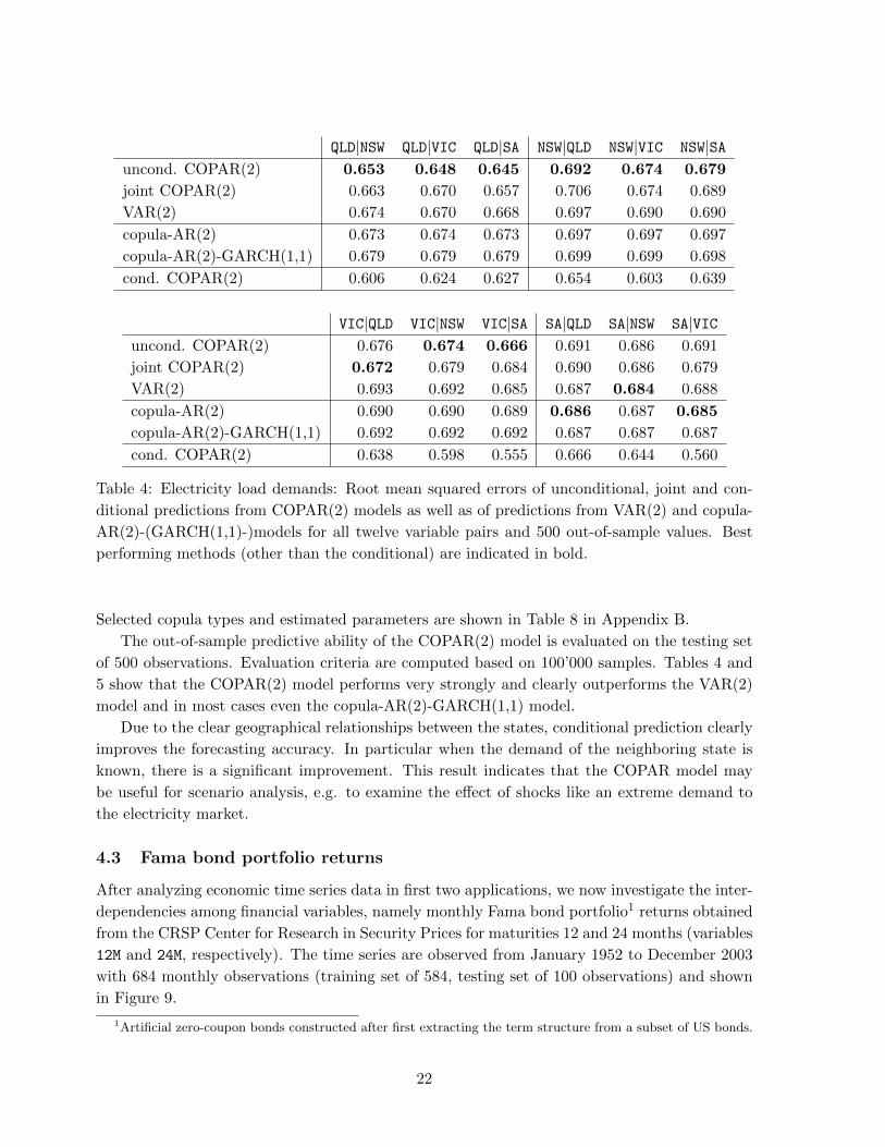
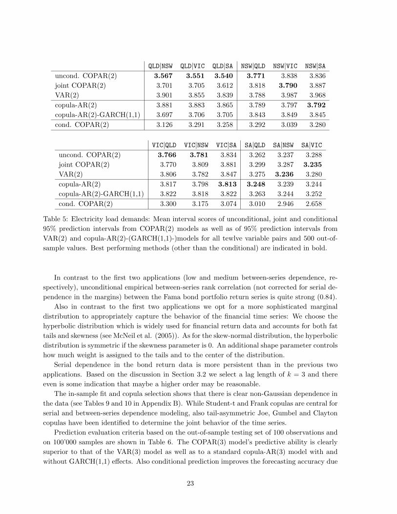
The out-of-sample predictive ability of the COPAR(2) model is evaluated on the testing set
of 500 observations. Evaluation criteria are computed based on 100’000 samples. Tables 4 and
5 show that the COPAR(2) model performs very strongly and clearly outperforms the VAR(2)
model and in most cases even the copula-AR(2)-GARCH(1,1) model.
Due to the clear geographical relationships between the states, conditional prediction clearly
improves the forecasting accuracy. In particular when the demand of the neighboring state is
known, there is a significant improvement. This result indicates that the COPAR model may
be useful for scenario analysis, e.g. to examine the effect of shocks like an extreme demand to
the electricity market.
4.3 Fama bond portfolio returns
After analyzing economic time series data in first two applications, we now investigate the inter-
dependencies among financial variables, namely monthly Fama bond portfolio1 returns obtained
from the CRSP Center for Research in Security Prices for maturities 12 and 24 months (variables
12M and 24M, respectively). The time series are observed from January 1952 to December 2003
with 684 monthly observations (training set of 584, testing set of 100 observations) and shown
in Figure 9.
1Artificial zero-coupon bonds constructed after first extracting the term structure from a subset of US bonds.
22
QLD|NSW QLD|VIC QLD|SA NSW|QLD NSW|VIC NSW|SAuncond. COPAR(2) 3.567 3.551 3.540 3.771 3.838 3.836
joint COPAR(2) 3.701 3.705 3.612 3.818 3.790 3.887
VAR(2) 3.901 3.855 3.839 3.788 3.987 3.968
copula-AR(2) 3.881 3.883 3.865 3.789 3.797 3.792
copula-AR(2)-GARCH(1,1) 3.697 3.706 3.705 3.843 3.849 3.845
cond. COPAR(2) 3.126 3.291 3.258 3.292 3.039 3.280
VIC|QLD VIC|NSW VIC|SA SA|QLD SA|NSW SA|VICuncond. COPAR(2) 3.766 3.781 3.834 3.262 3.237 3.288
joint COPAR(2) 3.770 3.809 3.881 3.299 3.287 3.235
VAR(2) 3.806 3.782 3.847 3.275 3.236 3.280
copula-AR(2) 3.817 3.798 3.813 3.248 3.239 3.244
copula-AR(2)-GARCH(1,1) 3.822 3.818 3.822 3.263 3.244 3.252
cond. COPAR(2) 3.300 3.175 3.074 3.010 2.946 2.658
Table 5: Electricity load demands: Mean interval scores of unconditional, joint and conditional
95% prediction intervals from COPAR(2) models as well as of 95% prediction intervals from
VAR(2) and copula-AR(2)-(GARCH(1,1)-)models for all tewlve variable pairs and 500 out-of-
sample values. Best performing methods (other than the conditional) are indicated in bold.
In contrast to the first two applications (low and medium between-series dependence, re-
spectively), unconditional empirical between-series rank correlation (not corrected for serial de-
pendence in the margins) between the Fama bond portfolio return series is quite strong (0.84).
Also in contrast to the first two applications we opt for a more sophisticated marginal
distribution to appropriately capture the behavior of the financial time series: We choose the
hyperbolic distribution which is widely used for financial return data and accounts for both fat
tails and skewness (see McNeil et al. (2005)). As for the skew-normal distribution, the hyperbolic
distribution is symmetric if the skewness parameter is 0. An additional shape parameter controls
how much weight is assigned to the tails and to the center of the distribution.
Serial dependence in the bond return data is more persistent than in the previous two
applications. Based on the discussion in Section 3.2 we select a lag length of k = 3 and there
even is some indication that maybe a higher order may be reasonable.
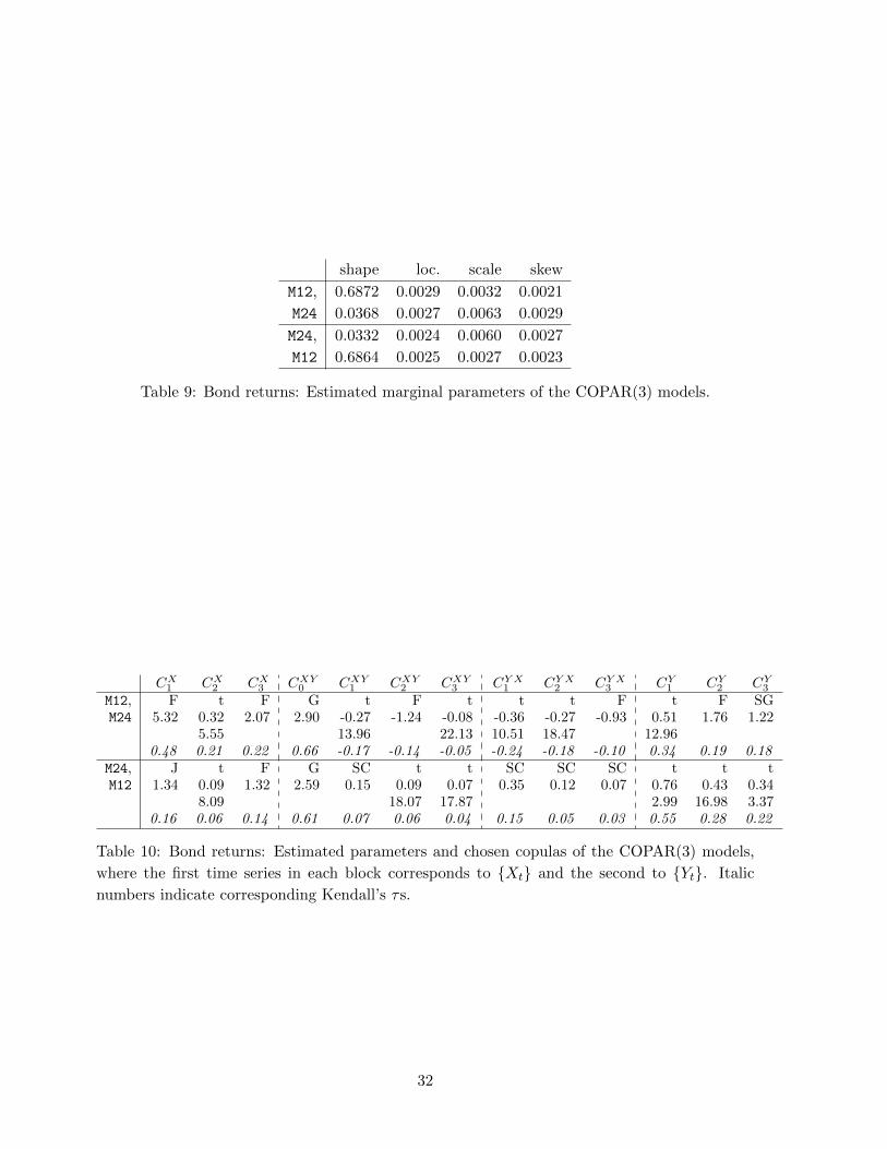
The in-sample fit and copula selection shows that there is clear non-Gaussian dependence in
the data (see Tables 9 and 10 in Appendix B). While Student-t and Frank copulas are central for
serial and between-series dependence modeling, also tail-asymmetric Joe, Gumbel and Clayton
copulas have been identified to determine the joint behavior of the time series.
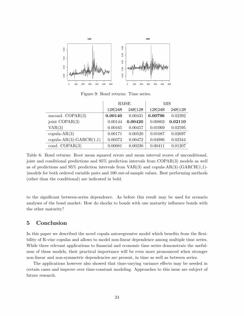
Prediction evaluation criteria based on the out-of-sample testing set of 100 observations and
on 100’000 samples are shown in Table 6. The COPAR(3) model’s predictive ability is clearly
superior to that of the VAR(3) model as well as to a standard copula-AR(3) model with and
without GARCH(1,1) effects. Also conditional prediction improves the forecasting accuracy due
23
0 100 200 300 400 500 600
0.00
0.01
0.02
0.03
12M
0 100 200 300 400 500 600
−0.
020.
000.
020.
040.
06
24M
Figure 9: Bond returns: Time series.
RMSE MIS
12M|24M 24M|12M 12M|24M 24M|12Muncond. COPAR(3) 0.00140 0.00431 0.00796 0.02392
joint COPAR(3) 0.00144 0.00420 0.00803 0.02110
VAR(3) 0.00165 0.00457 0.01069 0.02595
copula-AR(3) 0.00171 0.00520 0.01087 0.02697
copula-AR(3)-GARCH(1,1) 0.00372 0.00472 0.04986 0.02344
cond. COPAR(3) 0.00081 0.00230 0.00411 0.01207
Table 6: Bond returns: Root mean squared errors and mean interval scores of unconditional,
joint and conditional predictions and 95% prediction intervals from COPAR(3) models as well
as of predictions and 95% prediction intervals from VAR(3) and copula-AR(3)-(GARCH(1,1)-
)models for both ordered variable pairs and 100 out-of-sample values. Best performing methods
(other than the conditional) are indicated in bold.
to the significant between-series dependence. As before this result may be used for scenario
analyses of the bond market: How do shocks to bonds with one maturity influence bonds with
the other maturity?
5 Conclusion
In this paper we described the novel copula autoregressive model which benefits from the flexi-
bility of R-vine copulas and allows to model non-linear dependence among multiple time series.
While three relevant applications to financial and economic time series demonstrate the useful-
ness of these models, their practical importance will be even more pronounced when stronger
non-linear and non-symmetric dependencies are present, in time as well as between series.
The applications however also showed that time-varying variance effects may be needed in
certain cases and improve over time-constant modeling. Approaches to this issue are subject of
future research.
24
References
Aas, K., C. Czado, A. Frigessi, and H. Bakken (2009). Pair-copula constructions of multiple
dependence. Insurance: Mathematics and Economics 44 (2), 182–198.
Azzalini, A. (1985). A class of distributions which includes the normal ones. Scandinavian
Journal of Statistics 12, 171–178.
Bedford, T. and R. M. Cooke (2001). Probability density decomposition for conditionally
dependent random variables modeled by vines. Annals of Mathematics and Artificial in-
telligence 32, 245–268.
Bedford, T. and R. M. Cooke (2002). Vines - a new graphical model for dependent random
variables. Annals of Statistics 30, 1031–1068.
Brechmann, E. C., C. Czado, and K. Aas (2012). Truncated regular vines and their applica-
tions. Canadian Journal of Statistics 40 (1), 68–85.
Dißmann, J., E. C. Brechmann, C. Czado, and D. Kurowicka (2012). Selecting and es-
timating regular vine copulae and application to financial returns. Submitted preprint .
http://arxiv.org/abs/1202.2002.
Gneiting, T. and A. E. Raftery (2007). Strictly proper scoring rules, prediction, and estima-
tion. Journal of the American Statistical Association 102, 359–378.
Hamilton, J. D. (1994). Time Series Analysis. Princeton: Princeton Univerity Press.
Joe, H. (1996). Families of m-variate distributions with given margins and m(m−1)/2 bivari-
ate dependence parameters. In L. Ruschendorf, B. Schweizer, and M. D. Taylor (Eds.),
Distributions with Fixed Marginals and Related Topics, pp. 120–141. Hayward: Institute
of Mathematical Statistics.
Joe, H. (1997). Multivariate Models and Dependence Concepts. London: Chapman & Hall.
Joe, H. and J. Xu (1996). The estimation method of inference functions for margins for
multivariate models. Technical Report 166, Department of Statistics, University of British
Columbia.
Kurowicka, D. and R. M. Cooke (2006). Uncertainty Analysis with High Dimensional Depen-
dence Modelling. Chichester: John Wiley.
Kurowicka, D. and H. Joe (2011). Dependence Modeling: Vine Copula Handbook. Singapore:
World Scientific Publishing Co.
Lee, B.-S. (1992). Causal relations among stock returns, interest rates, real activity, and
inflation. Journal of Finance 47 (4), 1591–1603.
Lutkepohl, H. (2005). New Introduction to Multiple Time Series Analysis. Berlin: Springer.
McNeil, A. J., R. Frey, and P. Embrechts (2005). Quantitative Risk Management: Concepts
Techniques and Tools. Princeton: Princeton University Press.
Morales-Napoles, O. (2011). Counting vines. In D. Kurowicka and H. Joe (Eds.), Dependence
Modeling: Vine Copula Handbook. World Scientific Publishing Co.
25
Nelsen, R. B. (2006). An Introduction to Copulas (2nd ed.). Berlin: Springer.
Pfaff, B. (2008). VAR, SVAR and SVEC models: Implementation within R package vars.
Journal of Statistical Software 27 (4).
Sims, C. A. (1980). Macroeconomics and reality. Econometrica 48 (1), 1–48.
Sklar, A. (1959). Fonctions de repartition a n dimensions et leurs marges. Publications de
l’Institut de Statistique de L’Universite de Paris 8, 229–231.
Smith, M., A. Min, C. Czado, and C. Almeida (2010). Modeling longitudinal data using a
pair-copula decomposition of serial dependence. Journal of the American Statistical Asso-
ciation 105 (492), 1467–1479.
Tsay, R. S. (2002). Analysis of Financial Time Series. New York: Wiley.
Vuong, Q. H. (1989). Ratio tests for model selection and non-nested hypotheses. Economet-
rica 57 (2), 307–333.
Zivot, E. and J. Wang (2006). Modeling Financial Time Series with S-PLUS (2nd ed.). New
York: Springer.
26
A Technical supplement
As noted in Section 3.2 sequential copula selection and likelihood computation is not straight-
forward in the COPAR model. Figure 4 illustrates the interdependencies among the copulas.
For likelihood computation, of course the R-vine matrix specification (3.8) could be used in-
stead. However, given that the number of time points T might be large, evaluation of this
2T -by-2T -matrix is computationally rather inefficient, since most matrix entries do not contain
any information due to the assumed autoregressive order (see Example 3.7).
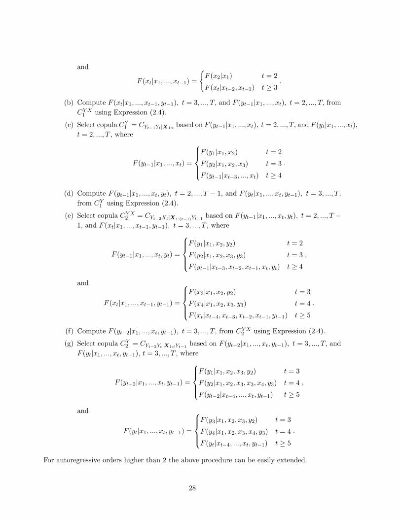
In the following we therefore present how to sequentially select copulas in a COPAR(2) model
for data {xt}t=1,...,T and {yt}t=1,...,T . Rather than selecting copulas, preliminarily determined
copulas can be estimated or likelihoods can be evaluated by simply altering the respective lines.
(i) Serial dependence of {Xt}t=1,...,T : Xs, Xt|Xs+1, ..., Xt−1, 1 ≤ s < t ≤ T .
(a) Select copula CX1 = CXt−1Xt based on {FX(xt)}t=1,...,T−1 and {F (xt)}t=2,...,T .
(b) Compute F (xt|xt−1), t = 3, ..., T, and F (xt−1|xt), t = 2, ..., T, from CX1 using Ex-
pression (2.4).
(c) Select copula CX2 = CXt−2Xt|Xt−1based on F (xt−1|xt), t = 2, ..., T−1, and F (xt|xt−1),
t = 3, ..., T .
(d) Compute F (xt−2|xt−1, xt), t = 3, ..., T, and F (xt|xt−2, xt−1), t = 3, ..., T, from CX2using Expression (2.4).
(ii) Between-series dependence Xs, Yt|Xs+1, ..., Xt, 1 ≤ s ≤ t ≤ T .
(a) Select copula CXY0 = CXtYt based on {FX(xt)}t=1,...,T and {FY (yt)}t=1,...,T .
(b) Compute F (yt|xt), t = 2, ..., T, from CXY0 using Expression (2.4).
(c) Select copula CXY1 = CXt−1Yt|Xtbased on F (xt−1|xt), t = 2, ..., T, and F (yt|xt), t =
2, ..., T .
(d) Compute F (yt|xt−1, xt), t = 3, ..., T, from CXY1 using Expression (2.4).
(e) Select copula CXY2 = CXt−2Yt|X(t−1):tbased on F (xt−2|xt−1, xt), t = 3, ..., T, and
F (yt|xt−1, xt), t = 3, ..., T .
(f) Compute F (yt|xt−2, xt−1, xt), t = 3, ..., T − 1, from CXY2 using Expression (2.4).
(iii) Between-series dependence Ys, Xt|X1, ..., Xt−1, Ys+1, ..., Yt−1, 1 ≤ s < t ≤ T, and condi-
tional serial dependence of {Yt}t=1,...,T : Ys, Yt|X1, ..., Xt, Ys+1, ..., Yt−1, 1 ≤ s < t ≤ T .
(a) Select copula CY X1 = CYt−1Xt|X1:(t−1)based on F (yt|x1, ..., xt), t = 1, ..., T − 1, and
F (xt|x1, ..., xt−1), t = 2, ..., T , where
F (yt|x1, ..., xt) =
F (y1|x1) t = 1
F (y2|x1, x2) t = 2
F (yt|xt−2, xt−1, xt) t ≥ 3
,
27
and
F (xt|x1, ..., xt−1) =
{F (x2|x1) t = 2
F (xt|xt−2, xt−1) t ≥ 3.
(b) Compute F (xt|x1, ..., xt−1, yt−1), t = 3, ..., T, and F (yt−1|x1, ..., xt), t = 2, ..., T, from
CY X1 using Expression (2.4).
(c) Select copula CY1 = CYt−1Yt|X1:tbased on F (yt−1|x1, ..., xt), t = 2, ..., T, and F (yt|x1, ..., xt),
t = 2, ..., T , where
F (yt−1|x1, ..., xt) =
F (y1|x1, x2) t = 2
F (y2|x1, x2, x3) t = 3
F (yt−1|xt−3, ..., xt) t ≥ 4
.
(d) Compute F (yt−1|x1, ..., xt, yt), t = 2, ..., T − 1, and F (yt|x1, ..., xt, yt−1), t = 3, ..., T,
from CY1 using Expression (2.4).
(e) Select copula CY X2 = CYt−2Xt|X1:(t−1)Yt−1based on F (yt−1|x1, ..., xt, yt), t = 2, ..., T −
1, and F (xt|x1, ..., xt−1, yt−1), t = 3, ..., T , where
F (yt−1|x1, ..., xt, yt) =
F (y1|x1, x2, y2) t = 2
F (y2|x1, x2, x3, y3) t = 3
F (yt−1|xt−3, xt−2, xt−1, xt, yt) t ≥ 4
,
and
F (xt|x1, ..., xt−1, yt−1) =
F (x3|x1, x2, y2) t = 3
F (x4|x1, x2, x3, y3) t = 4
F (xt|xt−4, xt−3, xt−2, xt−1, yt−1) t ≥ 5
.
(f) Compute F (yt−2|x1, ..., xt, yt−1), t = 3, ..., T, from CY X2 using Expression (2.4).
(g) Select copula CY2 = CYt−2Yt|X1:tYt−1based on F (yt−2|x1, ..., xt, yt−1), t = 3, ..., T, and
F (yt|x1, ..., xt, yt−1), t = 3, ..., T , where
F (yt−2|x1, ..., xt, yt−1) =
F (y1|x1, x2, x3, y2) t = 3
F (y2|x1, x2, x3, x3, x4, y3) t = 4
F (yt−2|xt−4, ..., xt, yt−1) t ≥ 5
,
and
F (yt|x1, ..., xt, yt−1) =
F (y3|x1, x2, x3, y2) t = 3
F (y4|x1, x2, x3, x4, y3) t = 4
F (yt|xt−4, ..., xt, yt−1) t ≥ 5
.
For autoregressive orders higher than 2 the above procedure can be easily extended.
28
B Additional figures and tables
X1 X2 X3 X4 X5
Y1 Y2 Y3 Y4 Y5
X1, X2 X2, X3 X3, X4 X4, X5
X1, Y1 X2, Y2 X3, Y3 X4, Y4 X5, Y5
X1, X3|X2 X2, X4|X3 X3, X5|X4
Y1, X2|X1 X1, Y2|X2 X2, Y3|X3 X3, Y4|X4 X4, Y5|X5
X1, X4|X2:3 X2, X5|X3:4
Y1, Y2|X1:2 Y2, X3|X1:2 X1, Y3|X2:3 X2, Y4|X3:4 X3, Y5|X4:5
X1, X5|X2:4
Y1, X3|X1:2, Y2 Y2, Y3|X1:3 Y3, X4|X1:3 X1, Y4|X2:4 X2, Y5|X3:5
Y1, Y3|X1:3, Y2 Y2, X4|X1:3, Y3 Y3, Y4|X1:4 Y4, X5|X1:4 X1, Y5|X2:5
Y1, X4|X1:3,Y 2:3 Y2, Y4|X1:4, Y3 Y3, X5|X1:4, Y4 Y4, Y5|X1:5
Y1, Y4|X1:4,Y 2:3 Y2, X5|X1:4,Y 3:4 Y3, Y5|X1:5, Y4
Y1, X5|X1:4,Y 2:4 Y2, Y5|X1:5,Y 3:4
Figure 10: R-vine for X1, ..., X4, Y1, ..., Y4 extended to include X5 and Y5. Dashed lines indicate
additional edges to include X5, dotted those to include Y5.
29
Margins Copulasloc. scale skew CX
1 CX2 CXY
0 CXY1 CXY
2 CY X1 CY X
2 CY1 CY
2
MKT, 0.0352 0.0494 -1.8383 N F F SJ SJ C F F tRRF 0.0027 0.0027 -1.3316 0.26 -0.49 -0.12 1.01 1.01 0.02 -0.71 15.6 0.24
7.170.17 -0.05 -0.01 0.01 0.01 0.01 -0.08 0.77 0.16
MKT, 0.0352 0.0494 -1.8383 N F F N N N SC G tINF 5e-04 0.0049 2.679 0.25 -0.49 -1.02 -0.03 -0.06 -0.11 0.07 1.86 0.27
9.390.16 -0.05 -0.11 -0.02 -0.04 -0.07 0.03 0.46 0.18
MKT, 0.0352 0.0494 -1.8383 N F C SJ SG N N t FIPG -0.0016 0.0104 0.7242 0.25 -0.52 0.02 1.01 1.02 -0.07 -0.09 0.40 1.00
9.950.16 -0.06 0.01 0.01 0.02 -0.04 -0.06 0.26 0.11
RRF, 0.0027 0.0027 -1.3316 F t F t F SJ C N FMKT 0.0352 0.0494 -1.8383 15.52 0.23 0.21 0.04 -0.41 1.07 0.13 0.26 -0.41
6.71 13.950.77 0.15 0.02 0.02 -0.05 0.04 0.06 0.17 -0.05
RRF, 0.0029 0.0029 -1.3316 F t F t t F N G tINF 5e-04 0.005 2.679 15.42 0.28 -0.58 0.05 0.07 -1.28 -0.04 1.92 0.28
7.25 30 24.91 14.960.77 0.18 -0.06 0.03 0.04 -0.14 -0.03 0.48 0.18
RRF, 0.0028 0.0027 -1.3316 F t C N t C C t FIPG -0.0021 0.0104 0.7242 15.07 0.24 0.12 -0.05 -0.10 0.10 0.13 0.36 0.97
6.48 10.50 12.240.76 0.16 0.06 -0.03 -0.06 0.05 0.06 0.23 0.11
INF, 5e-04 0.0049 2.679 G t F F SC F N t FMKT 0.0352 0.0494 -1.8383 1.91 0.27 -1.62 -0.56 0.09 0.31 -0.05 0.21 -0.53
11.64 20.080.48 0.17 -0.18 -0.06 0.04 0.03 -0.03 0.13 -0.06
INF, 5e-04 0.0049 2.679 G t F t N F t t tRRF 0.0028 0.0027 -1.3316 1.95 0.26 -0.09 -0.06 -0.02 0.01 -0.09 0.93 0.16
12.18 30 17.43 4.61 4.620.49 0.17 -0.01 -0.04 -0.01 0.00 -0.06 0.77 0.10
INF, 6e-04 0.005 2.679 G t N N t F F t FIPG -0.0016 0.0104 0.7242 1.92 0.26 -0.09 -0.10 -0.09 0.14 -0.06 0.39 0.93
12.48 30.00 9.880.48 0.17 -0.05 -0.06 -0.06 0.02 -0.01 0.25 0.10
IPG, -0.0016 0.0105 0.7242 t F C N N SG SG N FMKT 0.0353 0.0488 -1.8383 0.39 1.03 0.04 -0.09 -0.10 1.03 1.09 0.25 -0.49
9.250.26 0.11 0.02 -0.06 -0.06 0.02 0.08 0.16 -0.05
IPG, -0.0021 0.0104 0.7242 t F C SJ SJ F t F SGRRF 0.0027 0.0027 -1.3316 0.39 1.01 0.03 1.01 1.03 -0.07 -0.08 15.16 1.17
8.48 8.880.26 0.11 0.02 0.01 0.02 -0.01 -0.05 0.76 0.14
IPG, -0.0021 0.0104 0.7242 t F N N N t F G tINF 5e-04 0.005 2.679 0.41 0.96 -0.09 -0.03 -0.03 -0.13 -0.71 1.91 0.26
10.31 30.00 12.170.27 0.11 -0.06 -0.02 -0.02 -0.08 -0.08 0.48 0.17
Table 7: Macro-economic indicators: Estimated parameters and chosen copulas of the CO-
PAR(2) models, where the first time series in each block corresponds to {Xt} and the second to
{Yt}. Italic numbers indicate corresponding Kendall’s τs.
30
Margins Copulasloc. scale skew CX
1 CX2 CXY
0 CXY1 CXY
2 CY X1 CY X
2 CY1 CY
2
QLD, 0.5347 1.1087 -0.6587 F F t F SC SC F F NNSW -0.8134 1.2549 1.0882 7.05 -0.55 0.37 -0.20 0.05 0.18 -0.14 5.63 -0.07
8.630.56 -0.06 0.24 -0.02 0.02 0.08 -0.02 0.49 -0.04
QLD, 0.5627 1.1083 -0.6831 F F SJ F F F N F NNSW -0.5783 1.0801 0.8359 7.03 -0.53 1.14 0.19 0.06 0.01 0.10 5.78 -0.12
0.56 -0.06 0.07 0.02 0.01 0.00 0.06 0.50 -0.08QLD, 0.647 1.1597 -0.8191 F F SJ N F F F G FSA -0.9021 1.4215 1.9323 7.05 -0.54 1.06 -0.02 -0.03 0.01 0.62 1.85 -0.53
0.56 -0.06 0.04 -0.01 0.00 0.00 0.07 0.46 -0.06NSW, -0.8824 1.315 1.1642 F F t t G F G t FQLD 0.7313 1.2351 -1.1263 6.46 -0.43 0.39 0.14 1.05 0.06 1.04 0.72 -0.52
9.47 18.29 13.810.54 -0.05 0.26 0.09 0.05 0.01 0.04 0.51 -0.06
NSW, -0.6892 1.2084 0.8284 F F t N F F t F FVIC -0.6653 1.113 1.0071 6.36 -0.64 0.44 -0.16 -0.03 2.29 -0.10 4.70 -0.58
6.99 13.730.53 -0.07 0.29 -0.1 0.00 0.24 -0.07 0.44 -0.06
NSW, -0.913 1.3292 1.2318 F F t F N N N t FSA -0.6843 1.1507 1.0412 6.43 -0.50 0.43 -0.51 0.01 0.35 -0.07 0.56 -0.55
5.57 8.650.54 -0.05 0.28 -0.06 0.01 0.22 -0.04 0.38 -0.06
VIC, -0.6205 1.0997 0.9191 F N SJ F N F C t FQLD 0.7381 1.2083 -1.0317 5.88 -0.11 1.17 -0.06 0.04 0.33 0.03 0.76 -0.64
9.180.51 -0.07 0.09 -0.01 0.03 0.04 0.02 0.55 -0.07
VIC, -0.5819 1.0952 0.8255 F N t t F N F F FNSW -0.7386 1.2001 1.0095 6.11 -0.12 0.43 0.31 0.47 -0.07 0.83 5.17 0.01
8.66 8.330.52 -0.07 0.28 0.20 0.05 -0.05 0.09 0.47 0.00
VIC, -0.6299 1.1162 0.9363 F N t N F t N G tSA -0.7868 1.2349 1.4554 5.87 -0.11 0.67 -0.09 0.26 0.23 -0.12 1.48 -0.03
24.46 14.38 14.370.51 -0.07 0.47 -0.06 0.03 0.15 -0.08 0.32 -0.02
SA, -0.526 1.0738 0.8463 t N SJ F F F SC t FQLD 0.7778 1.2763 -1.1955 0.63 -0.07 1.07 0.01 0.37 0.00 0.09 0.76 -0.56
10.76 10.110.43 -0.05 0.04 0.00 0.04 0.00 0.04 0.55 -0.06
SA, -0.6242 1.1364 1.0308 t N t N F N N F CNSW -0.758 1.2212 1.079 0.63 -0.07 0.30 0.31 0.72 -0.04 0.08 5.28 0.01
10.76 5.300.44 -0.05 0.19 0.20 0.08 -0.03 0.05 0.47 0.01
SA, -0.5563 1.0947 0.8318 t N t t F N SC F NVIC -0.6184 1.0878 0.9467 0.64 -0.07 0.65 0.26 0.21 -0.04 0.05 4.47 -0.04
10.53 24.75 8.630.44 -0.05 0.45 0.17 0.02 -0.02 0.02 0.42 -0.02
Table 8: Electricity load demands: Estimated parameters and chosen copulas of the COPAR(2)
models, where the first time series in each block corresponds to {Xt} and the second to {Yt}.Italic numbers indicate corresponding Kendall’s τs.
31
shape loc. scale skew
M12, 0.6872 0.0029 0.0032 0.0021
M24 0.0368 0.0027 0.0063 0.0029
M24, 0.0332 0.0024 0.0060 0.0027
M12 0.6864 0.0025 0.0027 0.0023
Table 9: Bond returns: Estimated marginal parameters of the COPAR(3) models.
CX1 CX
2 CX3 CXY
0 CXY1 CXY
2 CXY3 CY X
1 CY X2 CY X
3 CY1 CY
2 CY3
M12, F t F G t F t t t F t F SGM24 5.32 0.32 2.07 2.90 -0.27 -1.24 -0.08 -0.36 -0.27 -0.93 0.51 1.76 1.22
5.55 13.96 22.13 10.51 18.47 12.960.48 0.21 0.22 0.66 -0.17 -0.14 -0.05 -0.24 -0.18 -0.10 0.34 0.19 0.18
M24, J t F G SC t t SC SC SC t t tM12 1.34 0.09 1.32 2.59 0.15 0.09 0.07 0.35 0.12 0.07 0.76 0.43 0.34
8.09 18.07 17.87 2.99 16.98 3.370.16 0.06 0.14 0.61 0.07 0.06 0.04 0.15 0.05 0.03 0.55 0.28 0.22
Table 10: Bond returns: Estimated parameters and chosen copulas of the COPAR(3) models,
where the first time series in each block corresponds to {Xt} and the second to {Yt}. Italic
numbers indicate corresponding Kendall’s τs.
32