Copula Based Factorization

in Bayesian Multivariate Infinite Mixture Models∗

Martin Burda† Artem Prokhorov‡

November 30, 2013

Abstract

Bayesian nonparametric models based on infinite mixtures of density kernels have been recently gaining in

popularity due to their flexibility and feasibility of implementation even in complicated modeling scenarios.

However, these models have been rarely applied in more than one dimension. Indeed, implementation in

the multivariate case is inherently difficult due to the rapidly increasing number of parameters needed to

characterize the joint dependence structure accurately. In this paper, we propose a factorization scheme

of multivariate dependence structures based on the copula modeling framework, whereby each marginal

dimension in the mixing parameter space is modeled separately and the marginals are then linked by a non-

parametric random copula function. Specifically, we consider nonparametric univariate Gaussian mixtures

for the marginals and a multivariate random Bernstein polynomial copula for the link function, under the

Dirichlet process prior. We show that in a multivariate setting this scheme leads to an improvement in the

precision of a density estimate relative to the commonly used multivariate Gaussian mixture. We derive weak

posterior consistency of the copula-based mixing scheme for general kernel types under high-level conditions,

and strong posterior consistency for the specific Bernstein-Gaussian mixture model.

JEL: C11, C14, C63

Keywords: Nonparametric copula; nonparametric consistency; mixture modeling

∗We would like to thank the participants of the 6th Annual Bayesian Econometric Workshop of the Rimini Center

for Economic Analysis, Toronto, 2012, the Canadian Economics Association Conference meetings, HEC Montreal,

2013, the Canadian Econometrics Study Group meetings, Kitchener, ON, 2013, the Midwest Econometrics Group

meetings, Bloomington, IN 2013, the 19th International Panel Data Conference, London, UK, 2013 and the seminar

audience at the University of New South Wales for their insightful comments and suggestions. This work was

made possible by the facilities of the Shared Hierarchical Academic Research Computing Network (SHARCNET:

www.sharcnet.ca) and it was supported by grants from the Social Sciences and Humanities Research Council of

Canada (SSHRC: www.sshrc-crsh.gc.ca).†Department of Economics, University of Toronto, 150 St. George St., Toronto, ON M5S 3G7, Canada; Phone:

(416) 978-4479; Email: martin.burda@utoronto.ca‡Department of Economics, Concordia University, and CIREQ, 1455 de Maisonneuve Blvd West, Montreal, QC

H3G 1M8, Canada; Phone: (514) 848-2424 ext.3908; Email: artem.prokhorov@concordia.ca

1

1. Bayesian Nonparametric Copula Kernel Mixture

Bayesian infinite mixture models are useful both as nonparametric estimation methods and as a way

of uncovering latent class structure that can explain the dependencies among the model variables.

Such models express a distribution as a mixture of simpler distributions without a priori restricting

the number of mixture components which is stochastic and data-driven. In many contexts, a

countably infinite mixture is also a more realistic model than a mixture with a small fixed number

of components.

Even though their theoretical foundations were developed early (Ferguson, 1973; Antoniak, 1974;

Lo, 1984), infinite mixture models have only recently become computationally feasible for practical

implementation on larger data sets with the development of Markov chain Monte Carlo (MCMC)

methods (Escobar and West, 1995; Neal, 2000). Bayesian infinite mixture models are becoming

increasingly popular. Among the many areas of applications are treatment effects (Chib and Hamil-

ton, 2002), autoregressive panel data (Hirano, 2002), finance (Jensen and Maheu, 2010), latent het-

erogeneity in discrete choice models (Kim, Menzefricke, and Feinberg, 2004; Burda, Harding, and

Hausman, 2008), contingent valuation models (Fiebig, Kohn, and Leslie, 2009), and instrumental

variables (Conley, Hansen, McCulloch, and Rossi, 2008). There is a growing number of applica-

tions in pattern recognition and other fields of machine learning (see, e.g., Fan and Bouguila, 2013),

in biology (see, e.g., Lartillot, Rodrigue, Stubbs, and Richer, 2013), in network traffic (see, e.g.,

Ahmed, Song, Nguyen, and Han, 2012), in DNA profiling (see, e.g., Zhang, Meng, Liu, and Huang,

2012), and other fields.

Most of these applications are univariate, or structured as conditionally independent copies of the

univariate case, albeit in some fields, such as machine learning, infinite mixture models have been

used in fairly high dimensions. Fundamentally, the computational complexity associated with algo-

rithms based on popular nonparametric priors, such as the Dirichlet process, is not directly related

to the dimensionality of the problem. However, the rapid increase in the number of mixture com-

ponents required to represent a nonparametric dependence structure accurately in high dimensions

poses a practical problem at the implementation level.

From a practical point of view, Dirichlet process priors can facilitate the feasibility of implementa-

tion by selecting relatively few latent classes in each MCMC step. However, this sparsity is traded

off with the accuracy of estimation. The analyst does have the option to generate a large number of

latent class proposals by tightening the prior of the concentration parameter in the Dirichlet process

mixture. Nonetheless, many of the latent classes proposed in this way are likely to be specified

over regions of the parameter space that are only weakly supported by the data. Hence, they will

either not be accepted or quickly discarded during the MCMC run, leading to a noisy estimate.

2

The severity of the trade-off is further exacerbated with higher dimensions: few mixing components

can provide a very inaccurate representation of the data generating process, but strengthening the

prior to increase their number will yield a higher rejection rate.

From our practical experience, we can alleviate some of these problems by relaxing the joint para-

metric specification of the mixing kernel, such as in the case of the typically used multivariate

Gaussian kernel. If the joint parametric mixing kernel can be decomposed into flexible building

blocks, each of which can be parsimoniously determined with high probability strongly supported

by the data then we should expect to obtain a more accurate representation. However, decomposi-

tions by conditional expansions such as the Cholesky factorization of the covariance matrix of the

multivariate Gaussian kernel still preserve the joint parametric dependence structure of the kernel.

What is needed for our purpose is a decomposition of the dependence structure itself.

In this paper, we propose a copula-based factorization scheme for Bayesian nonparametric mixture

models whereby each marginal dimension in the mixing parameter space is modeled as a separate

mixture and these marginal models are then joined by a nonparametric copula function based on

random Bernstein polynomials. In the implementation, only a few latent classes are required for

each of the marginals, regardless of the overall number of dimensions. We show that this scheme

leads to an improvement in the precision of a density estimate in finite samples relative to mixtures

of Gaussian kernels, providing a suitable tool for applications requiring joint dependence modeling

in the multivariate setting. Bearing in mind Freedman’s (1963) result concerning a topologically

wide class of priors leading to inconsistent posteriors in Bayesian nonparametric models, we specify

the conditions under which our approach yields posterior consistency; both for weak topologies for

a general class of kernels and strong topologies for the specific case of random Bernstein polynomial

copula and Gaussian mixture marginals (Bernstein-Gaussian mixture).

In a related literature, Chen, Fan, and Tsyrennikov (2006) consider a copula sieve maximum like-

lihood estimator with a parametric copula and nonparametric marginals, while Panchenko and

Prokhorov (2012) analyze the converse problem, with parametric marginals and a nonparametric

copula. In contrast, our procedure is based on both nonparametric copula and marginals. More-

over, in our case the number of mixture components is stochastic and automatically selected during

the MCMC run, without the need for model selection optimization required for approaches based

on maximum likelihood.

Nonparametric copula-based mixture models have been analyzed in several specific contexts dis-

tinct from ours. Silva and Gramacy (2009) present various MCMC proposals for copula mixtures.

Fuentes, Henry, and Reich (2012) analyze a spatial Dirichlet process (DP) copula model based

on the stick-breaking DP representation. Rey and Roth (2012) introduce a copula mixture model

3

to perform dependency-seeking clustering when co-occurring samples from different data sources

are available. Their model features nonparametric marginals and a Gaussian copula with block-

diagonal correlation matrix. Rodriguez, Dunson, and Gelfand (2010) construct a stochastic process

where observations at different locations are dependent, but have a common marginal distribution.

Dependence across locations is introduced by using a latent Gaussian copula model, resulting in

a latent stick-breaking process. Parametric Bayesian copula models and their mixtures have also

been analyzed in Pitt, Chan, and Kohn (2006), Silva and Lopes (2008), Ausin and Lopes (2010),

Epifani and Lijoi (2010), Leisen and Lijoi (2011), Barrientos, Jara, and Quintana (2012), Giordani,

Mun, and Kohn (2012), and Wu, Wang, and Walker (2013), among others.

Posterior consistency1 can fail in infinite-dimensional spaces for quite well-behaved models even for

seemingly natural priors (Freedman, 1963; Diaconis and Freedman, 1986; Kim and Lee, 2001). In

particular, the condition of assigning positive prior probabilities in ”usual” neighborhoods of the

true parameter is not sufficient to ensure consistency. The implication of Freedman’s (1963) result

is that the collection of all possible ”good pairs” of true parameter values and priors which lead to

consistency is extremely narrow when the size is measured topologically. A set F is called meager

and considered to be topologically small if F can be expressed as a countable union of sets Ci,

i ≥ 1, whose closures Ci have empty interior. Freedman (1963) showed that the collection of the

”good pairs” is meager in the product space (Ghosal, 2010). It is therefore important to provide

the set of conditions that ensure a proposed nonparametric modeling scenario fits into the meager

collection in infinite-dimensional spaces.

For the Gaussian kernel and the Dirichlet Process prior of the mixing distribution, asymptotic

properties, such as consistency, and rate of convergence of the posterior distribution based on

kernel mixture priors were established by Ghosal, Ghosh, and Ramamoorthi (1999), Tokdar (2006),

and Ghosal and van der Vaart (2001, 2007). Similar results for Dirichlet mixture of Bernstein

polynomials were shown by Petrone and Wasserman (2002), Ghosal (2001) and Kruijer and van der

Vaart (2008). Petrone and Veronese (2010) derived consistency for general kernels under the strong

condition that the true density is exactly of the mixture type for some compactly supported mixing

distribution, or the true density itself is compactly supported and is approximated in terms of

Kullback-Leibler divergence by its convolution with the chosen kernel. Wu and Ghosal (2008,

1Although consistency is intrinsically a frequentist property, it implies an eventual agreement among Bayesianswith different priors. For a subjective Bayesian who dispenses of the notion of a true parameter, consistency has animportant connection with the stability of predictive distributions of future observations – a consistent posterior willtend to agree with calculations of other Bayesians using a different prior distribution in the sense of weak topology.For an objective Bayesian who assumes the existence of an unknown true model, consistency can be thought of asa validation of the Bayesian method as approaching the mechanism used to generate the data (Ghosal and van derVaart, 2011). As pointed out by a referee, our treatment of posterior consistency is concerned with the behaviorof the posterior with respect to draws from a fixed sampling distribution, and so can be viewed as frequentist style

asymptotics.

4

2010) established consistency for a class of location-scale kernels and kernels with bounded support.

Shen and Ghosal (2011) and Canale and Dunson (2011) showed consistency for DP location-scale

mixtures based on multivariate Gaussian kernel. We extend on these results by analyzing a kernel

composed of a copula density with location-scale marginals.

The remainder of the paper is organized as follows. In Section 2 we provide the details of the pro-

posed copula-based factorization scheme, along with a specific kernel choices of Gaussian mixtures

for the marginals and Bernstein random polynomial copula for the link function. In Section 3, we

derive posterior consistency in the weak topology for general classes of kernels under high level

conditions and the Bernstein-Gaussian case under low level conditions. In Section 3 we establish

strong posterior consistency for the Bernstein-Gaussian scenario. In Section 4 we present the results

of a Monte Carlo experiment, comparing the accuracy of estimation of a multivariate joint density

between our Bernstein-Gaussian copula mixture and the popular multivariate Gaussian mixture.

Section 5 concludes.

2. Factorization for Infinite Mixture Models

2.1. Setup

Throughout, we will use the notation and terminology of Wu and Ghosal (2008), henceforth WG,

where applicable. Let X be the sample space with elements x, Θ the space of the mixing parameter

θ, and Φ the space of the hyper parameter φ. Let D(X ) denote the space of probability measures F

on X . Denote byM(Θ) the space of probability measures on Θ and let P be the mixing distribution

on Θ with density p and a prior Π on M(Θ) with weak support supp(Π). Denote the prior for φ

by μ, and the support of μ by supp(μ), with μ independent of P. Let K(x; θ, φ) be a kernel on

X ×Θ×Φ, such that K(x; θ, φ) is a jointly measurable function with the property that for all θ ∈ Θ

and φ ∈ Φ, K(∙; θ, φ) is a probability density on X .

Π, μ and K(x; θ, φ) induce a prior on D(X ) via the map

(2.1) (φ, P ) 7→ fP,φ(x) ≡∫K(x; θ, φ)dP (θ)

(the so-called type II mixture prior in WG). Denote such composite prior by Π∗.

2.2. Copula Kernel

We consider a kernel with the structure

(2.2) K(x; θ, φ) = Kc(F (x; θm, φm); θc, φc)Km(x; θm, φm)

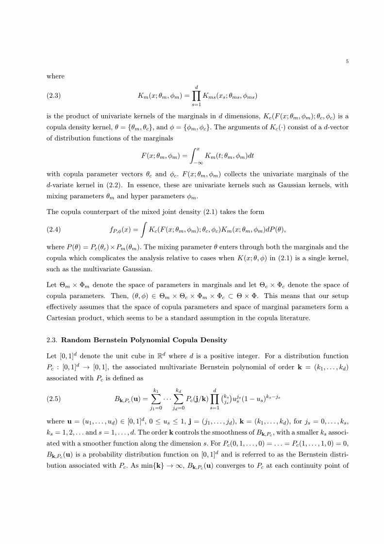
5

where

(2.3) Km(x; θm, φm) =d∏

s=1

Kms(xs; θms, φms)

is the product of univariate kernels of the marginals in d dimensions, Kc(F (x; θm, φm); θc, φc) is a

copula density kernel, θ = {θm, θc}, and φ = {φm, φc}. The arguments of Kc(∙) consist of a d-vector

of distribution functions of the marginals

F (x; θm, φm) =

∫ x

−∞Km(t; θm, φm)dt

with copula parameter vectors θc and φc. F (x; θm, φm) collects the univariate marginals of the

d-variate kernel in (2.2). In essence, these are univariate kernels such as Gaussian kernels, with

mixing parameters θm and hyper parameters φm.

The copula counterpart of the mixed joint density (2.1) takes the form

(2.4) fP,φ(x) =

∫Kc(F (x; θm, φm); θc, φc)Km(x; θm, φm)dP (θ),

where P (θ) = Pc(θc)×Pm(θm). The mixing parameter θ enters through both the marginals and the

copula which complicates the analysis relative to cases when K(x; θ, φ) in (2.1) is a single kernel,

such as the multivariate Gaussian.

Let Θm × Φm denote the space of parameters in marginals and let Θc × Φc denote the space of

copula parameters. Then, (θ, φ) ∈ Θm × Θc × Φm × Φc ⊂ Θ × Φ. This means that our setup

effectively assumes that the space of copula parameters and space of marginal parameters form a

Cartesian product, which seems to be a standard assumption in the copula literature.

2.3. Random Bernstein Polynomial Copula Density

Let [0, 1]d denote the unit cube in Rd where d is a positive integer. For a distribution function

Pc : [0, 1]d → [0, 1], the associated multivariate Bernstein polynomial of order k = (k1, . . . , kd)

associated with Pc is defined as

(2.5) Bk,Pc(u) =

k1∑

j1=0

∙ ∙ ∙kd∑

jd=0

Pc(j/k)d∏

s=1

(ksjs

)ujss (1− us)

ks−js

where u = (u1, . . . , ud) ∈ [0, 1]d, 0 ≤ us ≤ 1, j = (j1, . . . , jd), k = (k1, . . . , kd), for js = 0, . . . , ks,

ks = 1, 2, . . . and s = 1, . . . , d. The order k controls the smoothness of Bk,Pc , with a smaller ks associ-

ated with a smoother function along the dimension s. For Pc(0, 1, . . . , 0) = . . . = Pc(1, . . . , 1, 0) = 0,

Bk,Pc(u) is a probability distribution function on [0, 1]d and is referred to as the Bernstein distri-

bution associated with Pc. As min{k} → ∞, Bk,Pc(u) converges to Pc at each continuity point of

6

Pc and if Pc is continuous then the convergence is uniform on the unit cube [0, 1]d (Sancetta and

Satchell, 2004; Zheng, 2011).

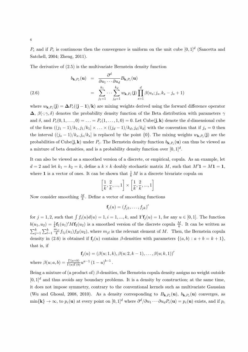
The derivative of (2.5) is the multivariate Bernstein density function

bk,Pc(u) =∂d

∂u1 ∙ ∙ ∙ ∂udBk,Pc(u)

=

k1∑

j1=1

∙ ∙ ∙kd∑

jd=1

wk,Pc(j)d∏

s=1

β(us; js, ks − js + 1)(2.6)

where wk,Pc(j) =ΔPc((j− 1)/k) are mixing weights derived using the forward difference operator

Δ, β(∙; γ, δ) denotes the probability density function of the Beta distribution with parameters γ

and δ, and Pc(0, 1, . . . , 0) = . . . = Pc(1, . . . , 1, 0) = 0. Let Cube(j,k) denote the d-dimensional cube

of the form ((j1 − 1)/k1, j1/k1]× . . . × ((jd − 1)/kd, jd/kd] with the convention that if js = 0 then

the interval ((js − 1)/ks, js/ks] is replaced by the point {0}. The mixing weights wk,Pc(j) are the

probabilities of Cube(j,k) under Pc. The Bernstein density function bk,Pc(u) can thus be viewed as

a mixture of beta densities, and is a probability density function over [0, 1]d.

It can also be viewed as a smoothed version of a discrete, or empirical, copula. As an example, let

d = 2 and let k1 = k2 = k, define a k × k doubly stochastic matrix M , such that M ′1 = M1 = 1,

where 1 is a vector of ones. It can be shown that 1k M is a discrete bivariate copula on[1

k,2

k, ..., 1

]

×

[1

k,2

k, ..., 1

]

Now consider smoothing Mk . Define a vector of smoothing functions

fj(u) = (fj1, . . . , fjk)′

for j = 1, 2, such that∫fi(u)d(u) = 1, i = 1, ..., k, and 1

′fj(u) = 1, for any u ∈ [0, 1]. The function

b(u1, u2) =1k f1(u1)

′M f2(u2) is a smoothed version of the discrete copulaMk . It can be written as∑k

j=1

∑kl=1

mjlk f1j(u1)f2l(u2), where mjl is the relevant element of M . Then, the Bernstein copula

density in (2.6) is obtained if fj(u) contains β-densities with parameters {(a, b) : a + b = k + 1},

that is, if

fj(u) = (β(u; 1, k), β(u; 2, k − 1), . . . , β(u; k, 1))′

where β(u; a, b) = Γ(a+b)Γ(a)Γ(b)u

a−1 (1− u)b−1 .

Being a mixture of (a product of) β-densities, the Bernstein copula density assigns no weight outside

[0, 1]d and thus avoids any boundary problems. It is a density by construction; at the same time,

it does not impose symmetry, contrary to the conventional kernels such as multivariate Gaussian

(Wu and Ghosal, 2008, 2010). As a density corresponding to Bk,Pc(u), bk,Pc(u) converges, as

min{k} → ∞, to pc(u) at every point on [0, 1]d where ∂d/∂u1 ∙ ∙ ∙ ∂udPc(u) = pc(u) exists, and if pc

7

is continuous and bounded then the convergence is uniform (Lorentz, 1986). Uniform approximation

results for the univariate and bivariate Bernstein density estimator can be found in Vitale (1975)

and Tenbusch (1994).

Petrone (1999a,b) proposed a class of prior distributions on the set of densities defined on [0, 1]

based on the univariate Bernstein polynomials and Petrone and Wasserman (2002) showed weak

and strong consistency of the Bernstein polynomial posterior for the space of univariate densities

on [0, 1]. Zheng, Zhu, and Roy (2010) and Zheng (2011) extended the settings to the multivariate

case, where k is an Nd-valued random variable and Pc is a random probability distribution function,

yielding Bk,Pc as a random function. A random Bernstein density bk,Pc(u) thus features random

mixing weights wk,Pc(j) with wk,Pc = {wk,Pc(j) : js = 1, . . . , ks, s = 1, . . . , d} belonging to the∏ds=1 ks − 1 dimensional simplex

sk =

wk,Pc(j) : wk,Pc(j) ≥ 0,

k1∑

j1=1

∙ ∙ ∙kd∑

jd=1

wk,Pc(j) = 1

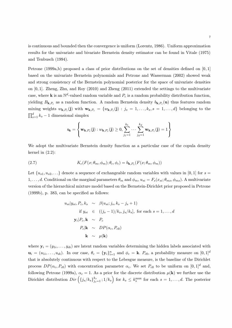
We adopt the multivariate Bernstein density function as a particular case of the copula density

kernel in (2.2):

(2.7) Kc(F (x; θm, φm); θc, φc) = bk,Pc(F (x; θm, φm))

Let {us1, us2, . . .} denote a sequence of exchangeable random variables with values in [0, 1] for s =

1, . . . , d. Conditional on the marginal parameters θm and φm, usi = Fs(xsi; θms, φms). A multivariate

version of the hierarchical mixture model based on the Bernstein-Dirichlet prior proposed in Petrone

(1999b), p. 383, can be specified as follows:

usi|ysi, Pc, ks ∼ β(usi; js, ks − js + 1)

if ysi ∈ ((js − 1)/ks, js/ks], for each s = 1, . . . , d

yi|Pc,k ∼ Pc

Pc|k ∼ DP (αc, Pc0)

k ∼ μ(k)

where yi = (y1i, . . . , ydi) are latent random variables determining the hidden labels associated with

ui = (u1i, . . . , udi). In our case, θc = {yi}ni=1 and φc = k. Pc0, a probability measure on [0, 1]d

that is absolutely continuous with respect to the Lebesgue measure, is the baseline of the Dirichlet

process DP (αc, Pc0) with concentration parameter αc. We set Pc0 to be uniform on [0, 1]d and,

following Petrone (1999a), αc = 1. As a prior for the discrete distribution μ(k) we further use the

Dirichlet distribution Dir({js/ks}

ksjs=1; 1/ks

)for ks ≤ kmaxs for each s = 1, . . . , d. The posterior

8

then follows directly from Petrone (1999a) who also proposes a sampling algorithm for the posterior

that we follow in the implementation.

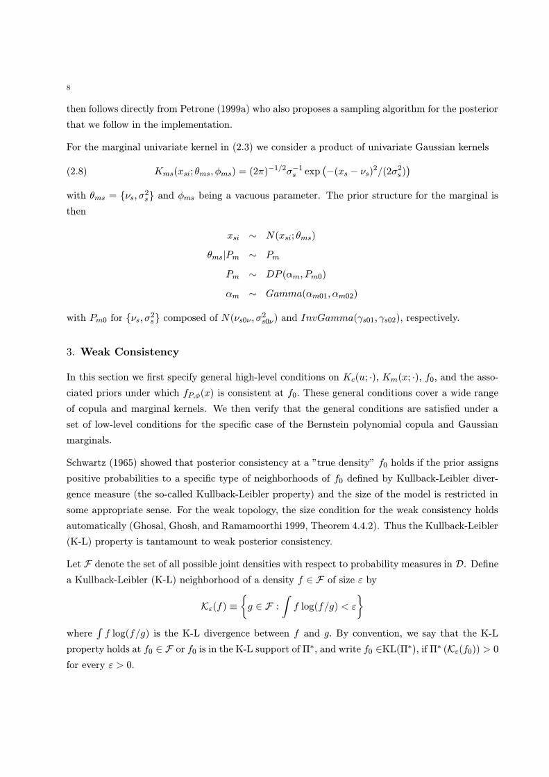
For the marginal univariate kernel in (2.3) we consider a product of univariate Gaussian kernels

(2.8) Kms(xsi; θms, φms) = (2π)−1/2σ−1s exp

(−(xs − νs)

2/(2σ2s))

with θms = {νs, σ2s} and φms being a vacuous parameter. The prior structure for the marginal is

then

xsi ∼ N(xsi; θms)

θms|Pm ∼ Pm

Pm ∼ DP (αm, Pm0)

αm ∼ Gamma(αm01, αm02)

with Pm0 for {νs, σ2s} composed of N(νs0ν , σ2s0ν) and InvGamma(γs01, γs02), respectively.

3. Weak Consistency

In this section we first specify general high-level conditions on Kc(u; ∙), Km(x; ∙), f0, and the asso-

ciated priors under which fP,φ(x) is consistent at f0. These general conditions cover a wide range

of copula and marginal kernels. We then verify that the general conditions are satisfied under a

set of low-level conditions for the specific case of the Bernstein polynomial copula and Gaussian

marginals.

Schwartz (1965) showed that posterior consistency at a ”true density” f0 holds if the prior assigns

positive probabilities to a specific type of neighborhoods of f0 defined by Kullback-Leibler diver-

gence measure (the so-called Kullback-Leibler property) and the size of the model is restricted in

some appropriate sense. For the weak topology, the size condition for the weak consistency holds

automatically (Ghosal, Ghosh, and Ramamoorthi 1999, Theorem 4.4.2). Thus the Kullback-Leibler

(K-L) property is tantamount to weak posterior consistency.

Let F denote the set of all possible joint densities with respect to probability measures in D. Define

a Kullback-Leibler (K-L) neighborhood of a density f ∈ F of size ε by

Kε(f) ≡

{

g ∈ F :∫f log(f/g) < ε

}

where∫f log(f/g) is the K-L divergence between f and g. By convention, we say that the K-L

property holds at f0 ∈ F or f0 is in the K-L support of Π∗, and write f0 ∈KL(Π∗), if Π∗ (Kε(f0)) > 0

for every ε > 0.

9

WG’s Theorem 1 and Lemmas 2 and 3 specify high-level conditions under which the K-L property

holds for a mixture density fP,φ(x) of the generic kernel K(x; θ, φ) in (2.1). They further show

that these conditions are satisfied under lower-level conditions for specific kernel types, such as the

location-scale kernel, gamma kernel, random histogram, and the Bernstein polynomial kernel.

Our analysis will proceed similarly by showing that the high-level conditions of WG’s Theorem 1 and

Lemmas 2 and 3 are satisfied for the copula kernel in (2.2). Our copula kernel is a composite function

of the special cases treated in WG – the location scale kernel and Bernstein polynomial kernel – in

that an integral of the former enters as an argument of the latter. Hence WG conditions derived

for each kernel separately need to be further developed and linked together to show consistency of

the resulting composite copula kernel which we do here. In Technical Appendix A, we restate WG

Theorem 1, and Lemmas 2 and 3 for the sake of completeness using our notation so that we can

seamlessly refer to the assumptions used by WG.

3.1. The K-L Property of a General Copula Mixture

The copula kernel Kc(∙) contains an integral expression and it is difficult to impose low-level con-

ditions on it directly without specifying its functional form. Hence we will state the following

Theorem in terms of relatively high-level conditions which will be subsequently verified for a spe-

cific functional form of the copula kernel. The Theorem can be somewhat loosely regarded as the

copula kernel counterpart of WG Theorem 2, but under higher-level conditions. Whenever φ and

θ share a common general prior, we will drop φ from the notation without loss of generality.

For any ε > 0, let Pε ∈ W ⊂ M(Θ) and φε ∈ A ⊂ Φ. In what follows φ will usually be subsumed

by θ, so instead of fPε,φε we will write fPε . Let f0(x) = fP0(x) denote the true density. Assume

the following set of conditions hold.

B1. For some 0 < f < ∞, 0 < f0(x) ≤ f for all x;

B2. For some 0 < p < ∞, 0 < p(θ) < p for all θ;

B3. Km(x; θm) is continuous in x, positive, bounded and bounded away from zero everywhere;

B4. Kc (∙) , Km(∙), log fPε(x), logKc (∙)Km(∙), and infθ∈D Kc (∙)Km(∙) are f0-integrable, the latter

for some closed D ⊃ supp(Pε);

B5. For some 0 < K <∞,∫Kc

(∫ x−∞Km(t; θm)dt; θc

)Km(x; θm)dθ = K for all x;

B6. The weak support of Π isM(Θ).

Condition B1 requires the true density to be bounded and bounded away from zero. Conditions B2

and B3 specify regularity conditions and f0-integrability of the kernels and their integrals. There is a

variety of different copula and location-scale kernel choices that satisfy these conditions. Conditions

10

B4 and B5 provide integrability and boundedness restrictions on the copula and marginal densities.

Condition B6 is relatively weak and does not make any specific assumptions on Π other than

requiring that it has large weak support. Thus, Π covers a wide class of priors including the

Dirichlet process.

Theorem 1. Let f0(x) be the true density and Π∗ an induced prior on F(X ) with the kernel

function

K(x; θ) = Kc

(∫ x

−∞Km(t; θm)dt; θc

)

Km(x; θm)

implying P ∼ Π, and given P, θ ∼ P. If Kc(∙), Km(∙), and f0(x) satisfy conditions B1–B6 then

f0 ∈KL(Π∗).

Proof of Theorem 1:

The proof is based on invoking WG Theorem 1, stated in Technical Appendix A, and showing that

its conditions A1 and A3 are met. Since in our Theorem 1 φ is subsumed as a part of θ, a separate

case for Condition A2 is redundant. To satisfy Condition A1, it suffices to show that for all r > r∗

with some r∗ <∞, there exists fPr(x) such that

(3.1) limr→∞

f0(x) logf0(x)

fPr(x)= 0

pointwise and that

(3.2)

∣∣∣∣f0(x) log

f0(x)

fPr(x)

∣∣∣∣ < C <∞.

Then, by the Dominated Convergence Theorem (DCT),

limr→∞

∫f0(x) log

f0(x)

fPr(x)dx = 0

which implies that Condition A1 is satisfied.

Now, define the probability density on a compact truncation of the parameter space as

(3.3) pr(θ) =

{vrp0(θ), ‖θ‖ < r, r ≥ 1

0, otherwise

and

v−1r =

∫

‖θ‖<rp0(θ)dθ,

Let Pr denote the probability measure corresponding to pr. Thus, by construction,

(3.4) limr→∞

pr(θ) = p0(θ)

Define

(3.5) fPr(x) =

∫Kc

(∫ x

−∞Km(t; θm)dt; θc

)

Km(x; θm)pr(θ)dθ

11

Using conditions B2, B3, and (3.4), another invocation of the DCT yields

(3.6) limr→∞

fPr(x) = fP0 ≡ f0(x)

pointwise in x for each θ. (3.6) then implies (3.1) using composition of limits and condition B1.

In order to show (3.2), we will provide bounds for the sequence fPr(x) in r. First, using (3.3) and

conditions B2 and B5,

fPr(x) = vr

∫

‖θ‖<rKc

(∫ x

−∞Km(t; θm)dt; θc

)

Km(x; θm)p(θ)dθ

< vrp

∫

‖θ‖<rKc

(∫ x

−∞Km(t; θm)dt; θc

)

Km(x; θm)dθ

≤ vrpK(3.7)

Due to (3.7), for all r, since fPr(x)→ f0(x) and vr → 1 as r →∞, there exists an r∗ such that for

all r > r∗,

(3.8)f0(x)

vrpK< 1

Combining (3.7) and (3.8),

(3.9) logf0(x)

fPr(x)≥ log

f0(x)

pvr

Second, by Conditions B2, B3 and (3.5) there exists a function g(x) such that fPr(x) ≥ g(x) > 0

for all r and x ∈ X , and hence

(3.10) logf0(x)

fPr(x)≤ log

f0(x)

g(x)

The inequalities (3.9) and (3.10) combined yield (3.2), thus completing verification of Condition

A1.

To show Condition A3, it suffices to verify conditions A7–A9 of WG Lemma 3, stated in Technical

Appendix A. Let Pε in the statement of WG Theorem 1, also provided in Technical Appendix A,

be chosen to be Pr which is compactly supported. By Condition B6, Pε ∈ supp(Π). Condition A7

is satisfied by condition B4. Condition A8 is satisfied by Condition B3. Condition A9 is satisfied

by condition B5. �

Now consider the case of the full copula kernel specification of (2.2) where φ = {φm, φc} is a

hyperparameter with prior μ = μm × μc separate from P. Assume that μ and P are a-priori

independently distributed. Now the prior Π∗ for density functions on X is induced by Π × μ via

the mapping (P, φ) 7→ fP,φ where fP,φ is given in (2.4). In this case condition B6 is replaced by the

following condition:

12

B6’. The weak support of Π isM(Θ× Φ).

Then the following Theorem applies:

Theorem 2. Under conditions B1-B5 and B6’, for fP,φ given in (2.4), f0 ∈KL(Π∗).

Proof of Theorem 2:

The proof of the theorem is virtually identical to the proof of Theorem 1 for verifying Conditions

A1 and A3. In contrast to Theorem 1, the weak support of Π is nowM(Θ×Φ) and the Condition

A2 of WG Theorem 1 now also needs to be satisfied. Condition A2 holds under conditions A4–A6

given WG Lemma 2, stated in Technical Appendix A. Conditions A4 and A5 are satisfied by our

Condition B6’. Condition A6 is satisfied by our Conditions B4 and B5. In summary, under the

Conditions A1–A3 we can now invoke WG Theorem 1 completing the proof. �

3.2. The K-L Property of the Random Bernstein Polynomial Copula

We will now show that the conditions B1–B5, and B6’ of Theorems 1 and 2 are satisfied by the

specific cases of the Bernstein random polynomials for the copula (2.7) along with the Gaussian

marginal kernel (2.8), under their respective priors. Condition B1 is assumed for the unknown

true density function and will be maintained throughout. Conditions B2 and B6’ are satisfied by

construction for the Dirichlet distribution and Dirichlet process priors considered. Condition B3 is

satisfied by the marginal Gaussian kernel provided that its variance stays strictly positive, which

is attained by the inverse gamma prior for the inverse variance. For Condition B4, f0-integrability

of Kc (∙) , Km(∙), log fPε(x), and logKc (∙)Km(∙) is given by the exponential tails of the Gaussian

Km(∙), compact support of Kc (∙) and a maintained assumption on f0. Integrability of Kc (∙)Km (∙)

with respect to θ in Condition B5 holds as long as the variance parameter in Km(∙) is strictly

positive, as specified by its prior.

4. Strong Consistency

The conditions discussed in previous section ensure weak convergence of the Bayesian estimate

of the density to the true density f0, that is, they guarantee that asymptotically the posterior

accumulates in weak neighborhoods of f0. However, as argued in Barron, Schervish and Wasserman

(1989), among others, there are many densities in the weak neighborhood that do not resemble f0

and consistency in a stronger sense is more appropriate.

13

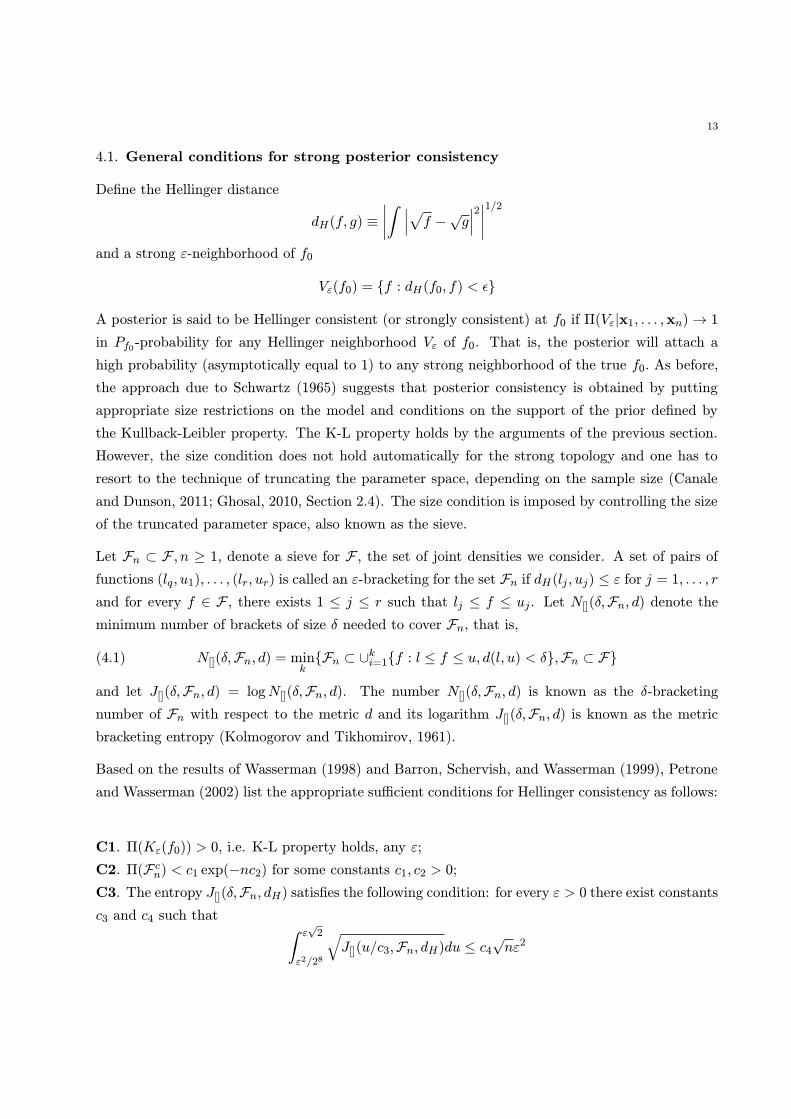
4.1. General conditions for strong posterior consistency

Define the Hellinger distance

dH(f, g) ≡

∣∣∣∣

∫ ∣∣∣√f −√g∣∣∣2∣∣∣∣

1/2

and a strong ε-neighborhood of f0

Vε(f0) = {f : dH(f0, f) < ε}

A posterior is said to be Hellinger consistent (or strongly consistent) at f0 if Π(Vε|x1, . . . ,xn)→ 1

in Pf0-probability for any Hellinger neighborhood Vε of f0. That is, the posterior will attach a

high probability (asymptotically equal to 1) to any strong neighborhood of the true f0. As before,

the approach due to Schwartz (1965) suggests that posterior consistency is obtained by putting

appropriate size restrictions on the model and conditions on the support of the prior defined by

the Kullback-Leibler property. The K-L property holds by the arguments of the previous section.

However, the size condition does not hold automatically for the strong topology and one has to

resort to the technique of truncating the parameter space, depending on the sample size (Canale

and Dunson, 2011; Ghosal, 2010, Section 2.4). The size condition is imposed by controlling the size

of the truncated parameter space, also known as the sieve.

Let Fn ⊂ F , n ≥ 1, denote a sieve for F , the set of joint densities we consider. A set of pairs of

functions (lq, u1), . . . , (lr, ur) is called an ε-bracketing for the set Fn if dH(lj , uj) ≤ ε for j = 1, . . . , r

and for every f ∈ F , there exists 1 ≤ j ≤ r such that lj ≤ f ≤ uj . Let N[](δ,Fn, d) denote the

minimum number of brackets of size δ needed to cover Fn, that is,

(4.1) N[](δ,Fn, d) = mink{Fn ⊂ ∪

ki=1{f : l ≤ f ≤ u, d(l, u) < δ},Fn ⊂ F}

and let J[](δ,Fn, d) = logN[](δ,Fn, d). The number N[](δ,Fn, d) is known as the δ-bracketing

number of Fn with respect to the metric d and its logarithm J[](δ,Fn, d) is known as the metric

bracketing entropy (Kolmogorov and Tikhomirov, 1961).

Based on the results of Wasserman (1998) and Barron, Schervish, and Wasserman (1999), Petrone

and Wasserman (2002) list the appropriate sufficient conditions for Hellinger consistency as follows:

C1. Π(Kε(f0)) > 0, i.e. K-L property holds, any ε;

C2. Π(Fcn) < c1 exp(−nc2) for some constants c1, c2 > 0;

C3. The entropy J[](δ,Fn, dH) satisfies the following condition: for every ε > 0 there exist constants

c3 and c4 such that∫ ε√2

ε2/28

√J[](u/c3,Fn, dH)du ≤ c4

√nε2

14

In essence these conditions (specifically, conditions C2 and C3) balance the size of the sieve Fn and

the prior probability of the sieve components Π(Fn): the integrated bracketing entropy of Fn has to

grow slower than linearly with√n, while the prior probability assigned outside Fn has to decrease

exponentially with n. Weaker conditions using covering numbers, rather than bracketing numbers,

are available from Ghosal, Ghosh, and Ramamoorthi (1999). However, since the bracketing number

bounds the covering number (Kosorok, 2008, p. 160-163), the fundamental idea of the balancing

between the size of the model and the prior probability assigned outside the sieve remains the same.

In the multivariate case, the metric entropy of the sieve components may quickly increase with

increasing dimensions. Wu and Ghosal (2010) and Canale and Dunson (2011) argue that this

substantially restricts the set of useable sieves in the multivariate setting: if the sieve is too small,

this will restrict the prior; if it is too large, this may lead to an exploding entropy. This makes it

difficult to provide general results on posterior consistency in multivariate settings. In what follows

we focus on the case of the Bernstein-Gaussian prior.

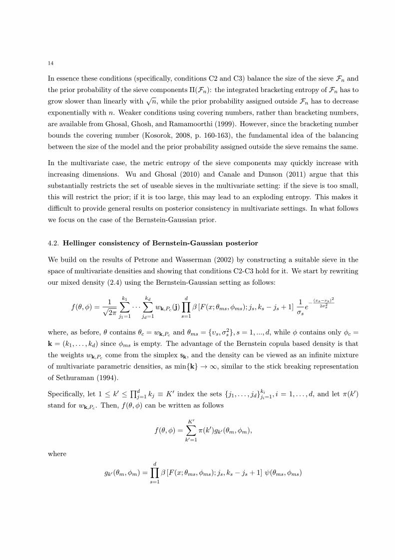
4.2. Hellinger consistency of Bernstein-Gaussian posterior

We build on the results of Petrone and Wasserman (2002) by constructing a suitable sieve in the

space of multivariate densities and showing that conditions C2-C3 hold for it. We start by rewriting

our mixed density (2.4) using the Bernstein-Gaussian setting as follows:

f(θ, φ) =1√2π

k1∑

j1=1

∙ ∙ ∙kd∑

jd=1

wk,Pc(j)d∏

s=1

β [F (x; θms, φms); js, ks − js + 1]1

σse− (xs−νs)

2

2σ2s

where, as before, θ contains θc = wk,Pc and θms = {υs, σ2s}, s = 1, ..., d, while φ contains only φc =

k = (k1, . . . , kd) since φms is empty. The advantage of the Bernstein copula based density is that

the weights wk,Pc come from the simplex sk, and the density can be viewed as an infinite mixture

of multivariate parametric densities, as min{k} → ∞, similar to the stick breaking representation

of Sethuraman (1994).

Specifically, let 1 ≤ k′ ≤∏dj=1 kj ≡ K ′ index the sets {j1, . . . , jd}

kiji=1

, i = 1, . . . , d, and let π(k′)

stand for wk,Pc . Then, f(θ, φ) can be written as follows

f(θ, φ) =

K′∑

k′=1

π(k′)gk′(θm, φm),

where

gk′(θm, φm) =d∏

s=1

β [F (x; θms, φms); js, ks − js + 1] ψ(θms, φms)

15

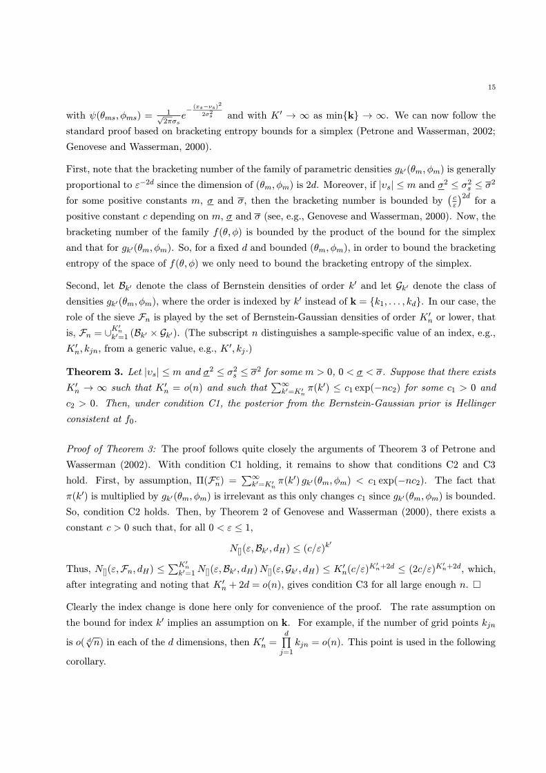
with ψ(θms, φms) =1√2πσs

e− (xs−νs)

2

2σ2s and with K ′ → ∞ as min{k} → ∞. We can now follow the

standard proof based on bracketing entropy bounds for a simplex (Petrone and Wasserman, 2002;

Genovese and Wasserman, 2000).

First, note that the bracketing number of the family of parametric densities gk′(θm, φm) is generally

proportional to ε−2d since the dimension of (θm, φm) is 2d. Moreover, if |υs| ≤ m and σ2 ≤ σ2s ≤ σ2

for some positive constants m, σ and σ, then the bracketing number is bounded by(cε

)2dfor a

positive constant c depending on m, σ and σ (see, e.g., Genovese and Wasserman, 2000). Now, the

bracketing number of the family f(θ, φ) is bounded by the product of the bound for the simplex

and that for gk′(θm, φm). So, for a fixed d and bounded (θm, φm), in order to bound the bracketing

entropy of the space of f(θ, φ) we only need to bound the bracketing entropy of the simplex.

Second, let Bk′ denote the class of Bernstein densities of order k′ and let Gk′ denote the class of

densities gk′(θm, φm), where the order is indexed by k′ instead of k = {k1, . . . , kd}. In our case, the

role of the sieve Fn is played by the set of Bernstein-Gaussian densities of order K ′n or lower, that

is, Fn = ∪K′nk′=1 (Bk′ × Gk′). (The subscript n distinguishes a sample-specific value of an index, e.g.,

K ′n, kjn, from a generic value, e.g., K′, kj .)

Theorem 3. Let |υs| ≤ m and σ2 ≤ σ2s ≤ σ2 for some m > 0, 0 < σ < σ. Suppose that there exists

K ′n → ∞ such that K′n = o(n) and such that

∑∞k′=K′n

π(k′) ≤ c1 exp(−nc2) for some c1 > 0 and

c2 > 0. Then, under condition C1, the posterior from the Bernstein-Gaussian prior is Hellinger

consistent at f0.

Proof of Theorem 3: The proof follows quite closely the arguments of Theorem 3 of Petrone and

Wasserman (2002). With condition C1 holding, it remains to show that conditions C2 and C3

hold. First, by assumption, Π(Fcn) =∑∞

k′=K′nπ(k′) gk′(θm, φm) < c1 exp(−nc2). The fact that

π(k′) is multiplied by gk′(θm, φm) is irrelevant as this only changes c1 since gk′(θm, φm) is bounded.

So, condition C2 holds. Then, by Theorem 2 of Genovese and Wasserman (2000), there exists a

constant c > 0 such that, for all 0 < ε ≤ 1,

N[](ε,Bk′ , dH) ≤ (c/ε)k′

Thus, N[](ε,Fn, dH) ≤∑K′n

k′=1N[](ε,Bk′ , dH)N[](ε,Gk′ , dH) ≤ K ′n(c/ε)K′n+2d ≤ (2c/ε)K

′n+2d, which,

after integrating and noting that K ′n + 2d = o(n), gives condition C3 for all large enough n. �

Clearly the index change is done here only for convenience of the proof. The rate assumption on

the bound for index k′ implies an assumption on k. For example, if the number of grid points kjn

is o( d√n) in each of the d dimensions, then K ′n =

d∏

j=1kjn = o(n). This point is used in the following

corollary.

16

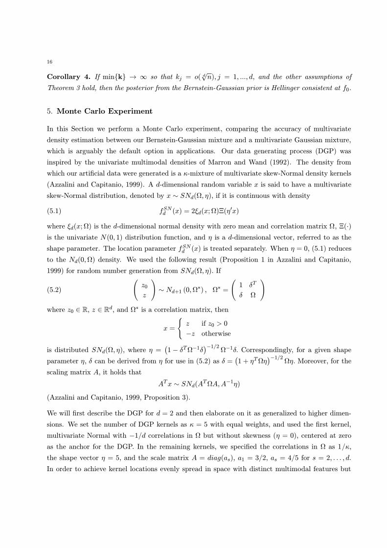
Corollary 4. If min{k} → ∞ so that kj = o( d√n), j = 1, ..., d, and the other assumptions of

Theorem 3 hold, then the posterior from the Bernstein-Gaussian prior is Hellinger consistent at f0.

5. Monte Carlo Experiment

In this Section we perform a Monte Carlo experiment, comparing the accuracy of multivariate

density estimation between our Bernstein-Gaussian mixture and a multivariate Gaussian mixture,

which is arguably the default option in applications. Our data generating process (DGP) was

inspired by the univariate multimodal densities of Marron and Wand (1992). The density from

which our artificial data were generated is a κ-mixture of multivariate skew-Normal density kernels

(Azzalini and Capitanio, 1999). A d-dimensional random variable x is said to have a multivariate

skew-Normal distribution, denoted by x ∼ SNd(Ω, η), if it is continuous with density

(5.1) fSNd (x) = 2ξd(x; Ω)Ξ(η′x)

where ξd(x; Ω) is the d-dimensional normal density with zero mean and correlation matrix Ω, Ξ(∙)

is the univariate N(0, 1) distribution function, and η is a d-dimensional vector, referred to as the

shape parameter. The location parameter fSNd (x) is treated separately. When η = 0, (5.1) reduces

to the Nd(0,Ω) density. We used the following result (Proposition 1 in Azzalini and Capitanio,

1999) for random number generation from SNd(Ω, η). If

(5.2)

(z0

z

)

∼ Nd+1 (0,Ω∗) , Ω∗ =

(1 δT

δ Ω

)

where z0 ∈ R, z ∈ Rd, and Ω∗ is a correlation matrix, then

x =

{z if z0 > 0

−z otherwise

is distributed SNd(Ω, η), where η =(1− δTΩ−1δ

)−1/2Ω−1δ. Correspondingly, for a given shape

parameter η, δ can be derived from η for use in (5.2) as δ =(1 + ηTΩη

)−1/2Ωη. Moreover, for the

scaling matrix A, it holds that

ATx ∼ SNd(ATΩA,A−1η)

(Azzalini and Capitanio, 1999, Proposition 3).

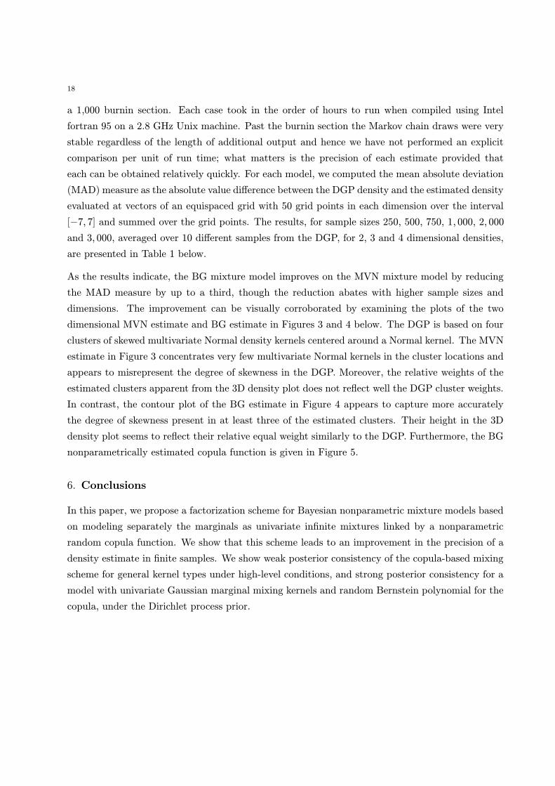
We will first describe the DGP for d = 2 and then elaborate on it as generalized to higher dimen-

sions. We set the number of DGP kernels as κ = 5 with equal weights, and used the first kernel,

multivariate Normal with −1/d correlations in Ω but without skewness (η = 0), centered at zero

as the anchor for the DGP. In the remaining kernels, we specified the correlations in Ω as 1/κ,

the shape vector η = 5, and the scale matrix A = diag(as), a1 = 3/2, as = 4/5 for s = 2, . . . , d.

In order to achieve kernel locations evenly spread in space with distinct multimodal features but

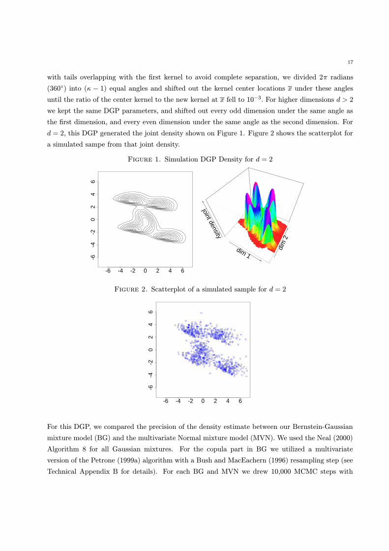
17

with tails overlapping with the first kernel to avoid complete separation, we divided 2π radians

(360◦) into (κ − 1) equal angles and shifted out the kernel center locations x under these angles

until the ratio of the center kernel to the new kernel at x fell to 10−3. For higher dimensions d > 2

we kept the same DGP parameters, and shifted out every odd dimension under the same angle as

the first dimension, and every even dimension under the same angle as the second dimension. For

d = 2, this DGP generated the joint density shown on Figure 1. Figure 2 shows the scatterplot for

a simulated sampe from that joint density.

Figure 1. Simulation DGP Density for d = 2

-6 -4 -2 0 2 4 6

-6-4

-20

24

6

dim 1

dim

2

joint density

Figure 2. Scatterplot of a simulated sample for d = 2

-6 -4 -2 0 2 4 6

-6-4

-20

24

6y

For this DGP, we compared the precision of the density estimate between our Bernstein-Gaussian

mixture model (BG) and the multivariate Normal mixture model (MVN). We used the Neal (2000)

Algorithm 8 for all Gaussian mixtures. For the copula part in BG we utilized a multivariate

version of the Petrone (1999a) algorithm with a Bush and MacEachern (1996) resampling step (see

Technical Appendix B for details). For each BG and MVN we drew 10,000 MCMC steps with

18

a 1,000 burnin section. Each case took in the order of hours to run when compiled using Intel

fortran 95 on a 2.8 GHz Unix machine. Past the burnin section the Markov chain draws were very

stable regardless of the length of additional output and hence we have not performed an explicit

comparison per unit of run time; what matters is the precision of each estimate provided that

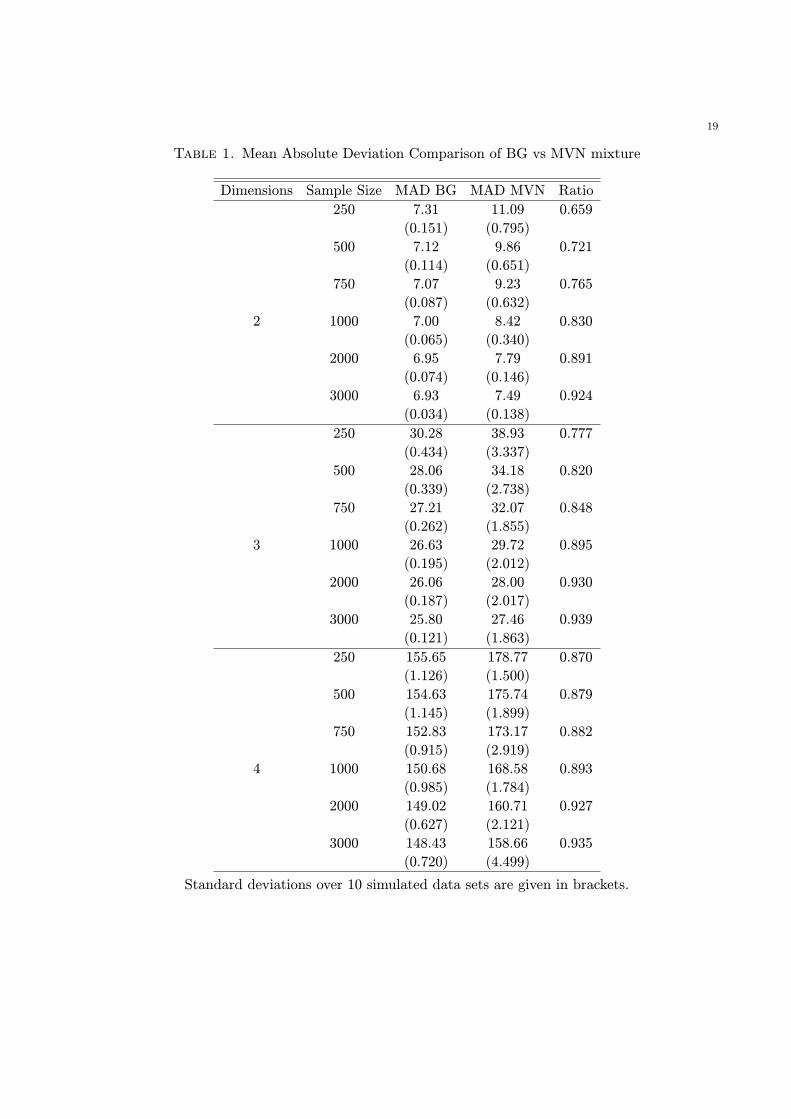
each can be obtained relatively quickly. For each model, we computed the mean absolute deviation

(MAD) measure as the absolute value difference between the DGP density and the estimated density

evaluated at vectors of an equispaced grid with 50 grid points in each dimension over the interval

[−7, 7] and summed over the grid points. The results, for sample sizes 250, 500, 750, 1, 000, 2, 000

and 3, 000, averaged over 10 different samples from the DGP, for 2, 3 and 4 dimensional densities,

are presented in Table 1 below.

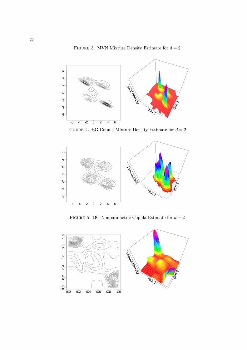
As the results indicate, the BG mixture model improves on the MVN mixture model by reducing

the MAD measure by up to a third, though the reduction abates with higher sample sizes and

dimensions. The improvement can be visually corroborated by examining the plots of the two

dimensional MVN estimate and BG estimate in Figures 3 and 4 below. The DGP is based on four

clusters of skewed multivariate Normal density kernels centered around a Normal kernel. The MVN

estimate in Figure 3 concentrates very few multivariate Normal kernels in the cluster locations and

appears to misrepresent the degree of skewness in the DGP. Moreover, the relative weights of the

estimated clusters apparent from the 3D density plot does not reflect well the DGP cluster weights.

In contrast, the contour plot of the BG estimate in Figure 4 appears to capture more accurately

the degree of skewness present in at least three of the estimated clusters. Their height in the 3D

density plot seems to reflect their relative equal weight similarly to the DGP. Furthermore, the BG

nonparametrically estimated copula function is given in Figure 5.

6. Conclusions

In this paper, we propose a factorization scheme for Bayesian nonparametric mixture models based

on modeling separately the marginals as univariate infinite mixtures linked by a nonparametric

random copula function. We show that this scheme leads to an improvement in the precision of a

density estimate in finite samples. We show weak posterior consistency of the copula-based mixing

scheme for general kernel types under high-level conditions, and strong posterior consistency for a

model with univariate Gaussian marginal mixing kernels and random Bernstein polynomial for the

copula, under the Dirichlet process prior.

19

Table 1. Mean Absolute Deviation Comparison of BG vs MVN mixture

Dimensions Sample Size MAD BG MAD MVN Ratio

250 7.31 11.09 0.659

(0.151) (0.795)

500 7.12 9.86 0.721

(0.114) (0.651)

750 7.07 9.23 0.765

(0.087) (0.632)

2 1000 7.00 8.42 0.830

(0.065) (0.340)

2000 6.95 7.79 0.891

(0.074) (0.146)

3000 6.93 7.49 0.924

(0.034) (0.138)

250 30.28 38.93 0.777

(0.434) (3.337)

500 28.06 34.18 0.820

(0.339) (2.738)

750 27.21 32.07 0.848

(0.262) (1.855)

3 1000 26.63 29.72 0.895

(0.195) (2.012)

2000 26.06 28.00 0.930

(0.187) (2.017)

3000 25.80 27.46 0.939

(0.121) (1.863)

250 155.65 178.77 0.870

(1.126) (1.500)

500 154.63 175.74 0.879

(1.145) (1.899)

750 152.83 173.17 0.882

(0.915) (2.919)

4 1000 150.68 168.58 0.893

(0.985) (1.784)

2000 149.02 160.71 0.927

(0.627) (2.121)

3000 148.43 158.66 0.935

(0.720) (4.499)

Standard deviations over 10 simulated data sets are given in brackets.

20

Figure 3. MVN Mixture Density Estimate for d = 2

-6 -4 -2 0 2 4 6

-6-4

-20

24

6

dim 1

dim

2

joint density

Figure 4. BG Copula Mixture Density Estimate for d = 2

-6 -4 -2 0 2 4 6

-6-4

-20

24

6

dim 1

dim

2

joint density

Figure 5. BG Nonparametric Copula Estimate for d = 2

0.0 0.2 0.4 0.6 0.8 1.0

0.0

0.2

0.4

0.6

0.8

1.0

dim 1

dim

2

copula density

21

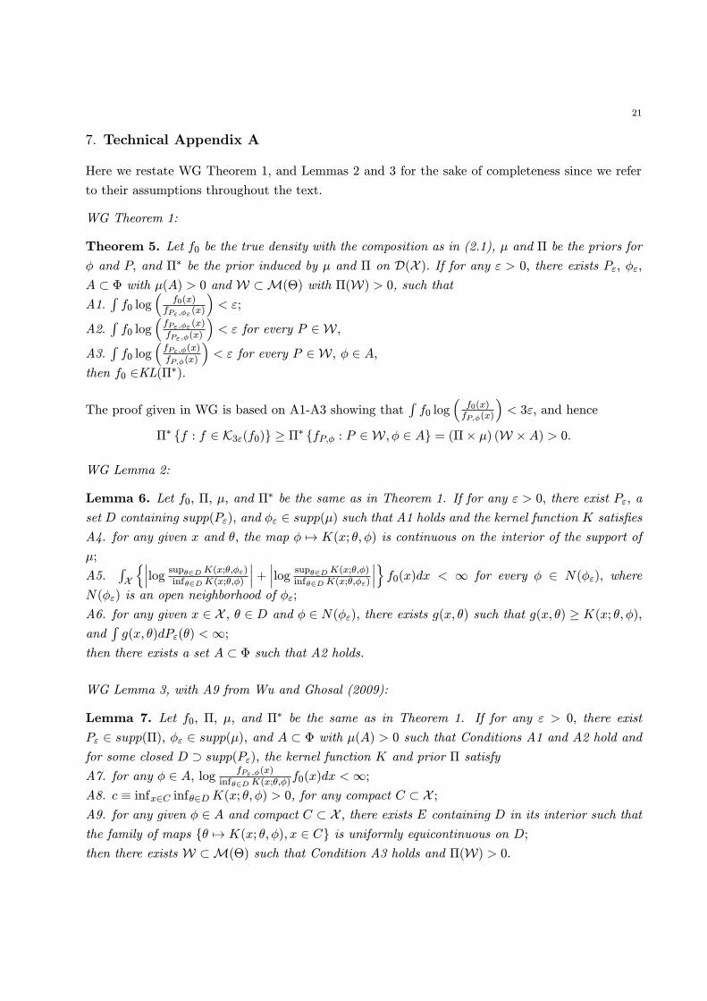
7. Technical Appendix A

Here we restate WG Theorem 1, and Lemmas 2 and 3 for the sake of completeness since we refer

to their assumptions throughout the text.

WG Theorem 1:

Theorem 5. Let f0 be the true density with the composition as in (2.1), μ and Π be the priors for

φ and P, and Π∗ be the prior induced by μ and Π on D(X ). If for any ε > 0, there exists Pε, φε,

A ⊂ Φ with μ(A) > 0 and W ⊂M(Θ) with Π(W) > 0, such that

A1.∫f0 log

(f0(x)

fPε,φε (x)

)< ε;

A2.∫f0 log

(fPε,φε (x)fPε,φ(x)

)< ε for every P ∈ W ,

A3.∫f0 log

(fPε,φ(x)fP,φ(x)

)< ε for every P ∈ W , φ ∈ A,

then f0 ∈KL(Π∗).

The proof given in WG is based on A1-A3 showing that∫f0 log

(f0(x)fP,φ(x)

)< 3ε, and hence

Π∗ {f : f ∈ K3ε(f0)} ≥ Π∗ {fP,φ : P ∈ W , φ ∈ A} = (Π× μ) (W ×A) > 0.

WG Lemma 2:

Lemma 6. Let f0, Π, μ, and Π∗ be the same as in Theorem 1. If for any ε > 0, there exist Pε, a

set D containing supp(Pε), and φε ∈ supp(μ) such that A1 holds and the kernel function K satisfies

A4. for any given x and θ, the map φ 7→ K(x; θ, φ) is continuous on the interior of the support of

μ;

A5.∫X

{∣∣∣log

supθ∈DK(x;θ,φε)infθ∈DK(x;θ,φ)

∣∣∣+∣∣∣log

supθ∈DK(x;θ,φ)infθ∈DK(x;θ,φε)

∣∣∣}f0(x)dx < ∞ for every φ ∈ N(φε), where

N(φε) is an open neighborhood of φε;

A6. for any given x ∈ X , θ ∈ D and φ ∈ N(φε), there exists g(x, θ) such that g(x, θ) ≥ K(x; θ, φ),

and∫g(x, θ)dPε(θ) <∞;

then there exists a set A ⊂ Φ such that A2 holds.

WG Lemma 3, with A9 from Wu and Ghosal (2009):

Lemma 7. Let f0, Π, μ, and Π∗ be the same as in Theorem 1. If for any ε > 0, there exist

Pε ∈ supp(Π), φε ∈ supp(μ), and A ⊂ Φ with μ(A) > 0 such that Conditions A1 and A2 hold and

for some closed D ⊃ supp(Pε), the kernel function K and prior Π satisfy

A7. for any φ ∈ A, log fPε,φ(x)infθ∈DK(x;θ,φ)

f0(x)dx <∞;

A8. c ≡ infx∈C infθ∈DK(x; θ, φ) > 0, for any compact C ⊂ X ;

A9. for any given φ ∈ A and compact C ⊂ X , there exists E containing D in its interior such that

the family of maps {θ 7→ K(x; θ, φ), x ∈ C} is uniformly equicontinuous on D;

then there exists W ⊂M(Θ) such that Condition A3 holds and Π(W) > 0.

22

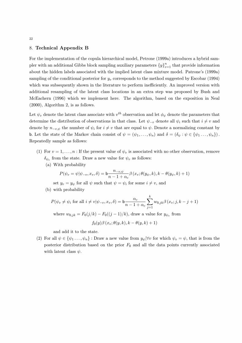
8. Technical Appendix B

For the implementation of the copula hierarchical model, Petrone (1999a) introduces a hybrid sam-

pler with an additional Gibbs block sampling auxiliary parameters {y}nv=1 that provide information

about the hidden labels associated with the implied latent class mixture model. Patrone’s (1999a)

sampling of the conditional posterior for yv corresponds to the method suggested by Escobar (1994)

which was subsequently shown in the literature to perform inefficiently. An improved version with

additional resampling of the latent class locations in an extra step was proposed by Bush and

McEachern (1996) which we implement here. The algorithm, based on the exposition in Neal

(2000), Algorithm 2, is as follows.

Let ψv denote the latent class associate with vth observation and let φψ denote the parameters that

determine the distribution of observations in that class. Let ψ−v denote all ψi such that i 6= v and

denote by n−v,ψ the number of ψi for i 6= v that are equal to ψ. Denote a normalizing constant by

b. Let the state of the Markov chain consist of ψ = (ψ1, . . . , ψn) and δ = (δψ : ψ ∈ {ψ1 . . . , ψn}) .

Repeatedly sample as follows:

(1) For v = 1, . . . , n : If the present value of ψv is associated with no other observation, remove

δψv from the state. Draw a new value for ψv as follows:

(a) With probability

P (ψv = ψ|ψ−v, xv, δ) = bn−v,ψ

n− 1 + αcβ (xv; θ(yψ, k), k − θ(yψ, k) + 1)

set yv = yψ for all ψ such that ψ = ψi for some i 6= v, and

(b) with probability

P (ψv 6= ψi for all i 6= v|ψ−v, xv, δ) = bαc

n− 1 + αc

k∑

j=1

w0,jkβ (xv; j, k − j + 1)

where w0,jk = F0(j/k)− F0((j − 1)/k), draw a value for yψv from

f0(y)β (xv; θ(y, k), k − θ(y, k) + 1)

and add it to the state.

(2) For all ψ ∈ {ψ1 . . . , ψn} : Draw a new value from yψ|∀v for which ψv = ψ, that is from the

posterior distribution based on the prior F0 and all the data points currently associated

with latent class ψ.

23

References

Ahmed, M., J. Song, N. Nguyen, and Z. Han (2012): “Nonparametric Bayesian identification of primary

users’ payloads in cognitive radio networks,” pp. 1586–1591.

Antoniak, C. E. (1974): “Mixtures of Dirichlet Processes with Applications to Bayesian Nonparametric

Problems,” The Annals of Statistics, 1, 1152–1174.

Ausin, M., and H. Lopes (2010): “Time-varying joint distribution through copulas,” Computational

Statistics and Data Analysis, 54(11), 2383–2399.

Barrientos, A. F., A. Jara, and F. A. Quintana (2012): “On the support of MacEachern’s dependent

Dirichlet processes and extensions,” Bayesian Analysis, 7(1), 1–34.

Barron, A., M. J. Schervish, and L. Wasserman (1999): “The Consistency of Posterior Distributions

in Nonparametric Problems,” The Annals of Statistics, 27(2), 536–561.

Burda, M., M. C. Harding, and J. A. Hausman (2008): “A Bayesian Mixed Logit-Probit Model for

Multinomial Choice,” Journal of Econometrics, 147(2), 232–246.

Canale, A., and D. B. Dunson (2011): “Bayesian multivariate mixed-scale density estimation,” working

paper, arXiv:1110.1265v2.

Chen, X., Y. Fan, and V. Tsyrennikov (2006): “Efficient Estimation of Semiparametric Multivariate

Copula Models,” Journal of the American Statistical Association, 101, 1228–1240.

Chib, S., and B. Hamilton (2002): “Semiparametric bayes analysis of longitudinal data treatment mod-

els,” Journal of Econometrics, 110, 67–89.

Conley, T., C. Hansen, R. McCulloch, and P. Rossi (2008): “A Semi-Parametric Bayesian Approach

to the Instrumental Variable Problem,” Journal of Econometrics, 144, 276–305.

Diaconis, P., and D. Freedman (1986): “On the Consistency of Bayes Estimates,” Annals of Statistics,

14(1), 1–26.

Epifani, I., and A. Lijoi (2010): “NONPARAMETRIC PRIORS FOR VECTORS OF SURVIVAL FUNC-

TIONS,” Statistica Sinica, 20, 1455–1484.

Escobar, M. D., and M. West (1995): “Bayesian Density Estimation and Inference Using Mixtures,”

Journal of the American Statistical Association, 90(430), 577–588.

Fan, W., and N. Bouguila (2013): “Variational learning of a Dirichlet process of generalized Dirichlet

distributions for simultaneous clustering and feature selection,” Pattern Recognition, 46(10), 2754–2769.

Ferguson, T. S. (1973): “A Bayesian Analysis of some Nonparametric Problems,” The Annals of Statistics,

1, 209–230.

Fiebig, D. G., R. Kohn, and D. S. Leslie (2009): “Nonparametric estimation of the distribution function

in contingent valuation models,” Bayesian Analysis, 4(3), 573–597.

Freedman, D. (1963): “On the asymptotic behavior of Bayes estimates in the discrete Markov processes,”

Annals of Mathematical Statistics, 34, 1386–1403.

Fuentes, M., J. Henry, and B. Reich (2012): “Nonparametric spatial models for extremes: application

to extreme temperature data,” Extremes, pp. 1–27.

Genovese, C., and L. Wasserman (2000): “Rates of convergence for the Gaussian mixture sieve,” The

Annals of Statistics, 28(4), 1105–1127.

24

Ghosal, S. (2001): “Convergence rates for density estimation with Bernstein polynomials,” Annals of

Statistics, 29(5), 1264–1280.

Ghosal, S. (2010): “The Dirichlet process, related priors and posterior asymptotics,” in Bayesian Non-

parametrics, ed. by N. L. Hjort, C. Holmes, P. Mueller, and S. G. Walker. Cambridge University Press.

Ghosal, S., J. K. Ghosh, and R. V. Ramamoorthi (1999): “Posterior Consistency of Dirichlet Mixtures

in Density Estimation,” The Annals of Statistics, 27(1), 143–158.

Ghosal, S., and A. van der Vaart (2001): “Entropies and rates of convergence for Bayes and maximum

likelihood estimation for mixture of normal densities,” Annals of Statistics, 29(5), 1233–1263.

(2007): “Posterior convergence rates of Dirichlet mixtures at smooth densities,” Annals of Statistics,

35(2), 697–723.

(2011): “Theory of Nonparametric Bayesian Inference,” Cambridge University Press.

Giordani, P., X. Mun, and R. Kohn (2012): “Efficient estimation of covariance matrices using posterior

mode multiple shrinkage,” Journal of Financial Econometrics, 11(1), 154–192.

Hirano, K. (2002): “Semiparametric bayesian inference in autoregressive panel data models,” Econometrica,

70, 781–799.

Jensen, M., and J. M. Maheu (2010): “Bayesian semiparametric stochastic volatility modeling,” Journal

of Econometrics, 157(2), 306–316.

Kim, J. G., U. Menzefricke, and F. Feinberg (2004): “Assessing Heterogeneity in Discrete Choice

Models Using a Dirichlet Process Prior,” Review of Marketing Science, 2(1), 1–39.

Kim, Y., and J. Lee (2001): “On posterior consistency of survival models,” Annals of Statistics, 29,

666–686.

Kolmogorov, A., and V. Tikhomirov (1961): “Epsilon-entropy and epsilon-capacity of sets in function

spaces,” AMS Translations Series 2 [Translated from Russian (1959) Uspekhi Mat.Nauk 14, 3-86], 17,

277–364.

Kosorok, M. (2008): Introduction to Empirical Processes and Semiparametric Inference, Springer Series

in Statistics. Springer.

Kruijer, W., and A. van der Vaart (2008): “Posterior convergence rates for Dirichlet mixtures of Beta

densities,” Journal of Statistical Planning and Inference, 138, 1981–1992.

Lartillot, N., N. Rodrigue, D. Stubbs, and J. Richer (2013): “Phylobayes mpi: Phylogenetic

reconstruction with infinite mixtures of profiles in a parallel environment,” Systematic Biology, 62(4),

611–615.

Leisen, F., and A. Lijoi (2011): “Vectors of two-parameter Poisson-Dirichlet processes,” Journal of

Multivariate Analysis, 102(3), 482–495.

Lo, A. Y. (1984): “On a class of Bayesian nonparametric estimates I: Density estimation,” Annals of

Statistics, 12, 351–357.

Lorentz, G. (1986): Bernstein Polynomials. University of Toronto Press.

Neal, R. M. (2000): “Markov Chain Sampling Methods for Dirichlet Process Mixture Models,” Journal of

Computational and Graphical Statistics, 9(2), 249–265.

Panchenko, V., and A. Prokhorov (2012): “Efficient Estimation of Parameters in Marginals,” Concor-

dia University Working Paper.

25

Petrone, S. (1999a): “Bayesian density estimation using bernstein polynomials,” Canadian Journal of

Statistics, 27(1), 105–126.

(1999b): “Random Bernstein Polynomials,” Scandinavian Journal of Statistics, 26(3), 373–393.

Petrone, S., and P. Veronese (2010): “Feller operators and mixture priors in Bayesian nonparametrics,”

Statistica Sinica, 20, 379–404.

Petrone, S., and L. Wasserman (2002): “Consistency of Bernstein Polynomial Posteriors,” Journal of

the Royal Statistical Society. Series B (Statistical Methodology), 64(1), 79–100.

Pitt, M., D. Chan, and R. Kohn (2006): “Efficient Bayesian inference for Gaussian copula regression

models,” Biometrika, 93(3), 537–554.

Rey, M., and V. Roth (2012): “Copula mixture model for dependency-seeking clustering,” in Proceedings

of the 29th International Conference on Machine Learning, pp. 927–934. ICML.

Rodriguez, A., D. Dunson, and A. Gelfand (2010): “Latent stick-breaking processes,” Journal of the

American Statistical Association, 105(490), 647–659.

Sancetta, A., and S. Satchell (2004): “The Bernstein Copula And Its Applications To Modeling And

Approximations Of Multivariate Distributions,” Econometric Theory, 20(03), 535–562.

Schwartz, L. (1965): “On Bayesian procedures,” Probability Theory and Related Fields (Z. Wahrschein-

lichkeitstheorie), 4, 10–26.

Sethuraman, J. (1994): “A constructive definition of Dirichlet priors,” Statistica Sinica, 4, 639–650.

Shen, W., and S. Ghosal (2011): “Adaptive Bayesian multivariate density estimation with Dirichlet

mixtures,” .

Silva, R., and R. B. Gramacy (2009): “MCMC Methods for Bayesian Mixtures of Copulas,” in Proceed-

ings of the 12th International Conference on Artificial Intelligence and Statistics 2009, Clearwater Beach,

Florida, USA, pp. 512–519.

Silva, R. d. S., and H. F. Lopes (2008): “Copula, marginal distributions and model selection: a Bayesian

note,” Statistics and Computing, 18, 313–320.

Tenbusch, A. (1994): “Two-dimensional Bernstein polynomial density estimators,” Metrika, 41(1), 233–

253, Metrika.

Tokdar, S. T. (2006): “Posterior Consistency of Dirichlet Location-scale Mixture of Normals in Density

Estimation and Regression,” Sankhya, 68, 90–110.

Vitale, R. (1975): “A Bernstein polynomial approach to density function estimation,” in Statistical infer-

ence and related topics, ed. by M. Puri.

Wasserman, L. (1998): “Asymptotic properties of nonparametric Bayesian procedures,” in Practical Non-

parametric and Semiparametric Bayesian Statistics, ed. by D. Dey, P. Mueller, and D. Sinha. Springer,

New York.

Wu, J., X. Wang, and S. Walker (2013): “Bayesian Nonparametric Inference for a Multivariate Copula

Function,” Methodology and Computing in Applied Probability, pp. 1–17, Article in Press.

Wu, Y., and S. Ghosal (2008): “Kullback Leibler property of kernel mixture priors in Bayesian density

estimation,” Electronic Journal of Statistics, 2, 298–331.

(2010): “The -consistency of Dirichlet mixtures in multivariate Bayesian density estimation,”

Journal of Multivariate Analysis, 101(10), 2411–2419.

26

Zhang, L., J. Meng, H. Liu, and Y. Huang (2012): “A nonparametric Bayesian approach for clustering

bisulfate-based DNA methylation profiles.,” BMC genomics, 13 Suppl 6.

Zheng, Y. (2011): “Shape restriction of the multi-dimensional Bernstein prior for density functions,” Sta-

tistics and Probability Letters, 81(6), 647–651.

Zheng, Y., J. Zhu, and A. Roy (2010): “Nonparametric Bayesian inference for the spectral density

function of a random field,” Biometrika, 97, 238–245.