Copula-based Multivariate GARCH Model withUncorrelated Dependent Errors∗

Tae-Hwy Lee†

University of California, RiversideXiangdong Long‡

University of Cambridge

August 2005

ABSTRACT

Multivariate GARCH (MGARCH) models are usually estimated under multivariate nor-mality. In this paper, for non-elliptically distributed financial returns, we propose copula-based multivariate GARCH (C-MGARCH) model with uncorrelated dependent errors, whichare generated through a linear combination of dependent random variables. The dependencestructure is controlled by a copula function. Our new C-MGARCH model nests a conven-tional MGARCH model as a special case. We apply this idea to the three MGARCH models,namely, the dynamic conditional correlation (DCC) model of Engle (2002), the varying cor-relation (VC) model of Tse and Tsui (2002), and the BEKK model of Engle and Kroner(1995). Monte Carlo experiment is conducted to illustrate the performance of C-MGARCHvs MGARCH models. Empirical analysis with a pair of the U.S. equity indices and twopairs of the foreign exchange rates indicates that the C-MGARCH models outperform DCC,VC, and BEKK in terms of in-sample model selection criteria (likelihood, AIC, SIC) andout-of-sample multivariate density forecast.

Key Words: Copula, Density forecast, Non-elliptical distribution, Predictive likelihood, Un-correlated dependent errors.

JEL Classification: C3, C5, G0.

∗Long thanks for the UCR Chancellor Fellowship.†Corresponding author. Department of Economics, University of California, Riverside, CA 92521, U.S.A.

Tel: +1 (951) 827-1509. Fax: +1 (951) 827-5685. Email: tae.lee@ucr.edu.‡Cambridge Endowment for Research in Finance, Judge Institute of Management, University of Cam-

bridge, U.K. Email: dxlecon@gmail.com.

1 Introduction

Modeling the conditional covariance matrix is in the core of financial econometrics, as it

is crucial for the asset allocation, financial risk management, and derivatives pricing. The

multivariate generalized autoregressive conditional heteroskedasticity (MGARCH) models in

the literature include the BEKK model by Engle and Kroner (1995), the dynamic conditional

correlation (DCC) model by Engel (2002), and the varying correlation (VC) model by Tse and

Tsui (2002). However, these models have been estimated under the multivariate normality

assumption, while this assumption has been rejected in much of the empirical findings —

Fama and French (1993), Richardson and Smith (1993), Longin and Solnik (2001), Mashal

and Zeevi (2002), among many others.

We propose a simple new model named a Copula-based Multivariate GARCH model,

or in short C-MGARCH model, which permits modeling conditional correlation and de-

pendence separately and simultaneously for interested financial returns with non-elliptically

distributed dependent errors. Our approach is based on a transformation, which removes

the linear correlation from the dependent variables to form uncorrelated dependent errors.

The dependence structure is controlled by a copula while the correlation is modeled by an

MGARCH model. The C-MGARCH model can capture the dependence in the uncorre-

lated errors ignored by all existing MGARCH models. For every MGARCH model, the

corresponding C-MGARCH model can be constructed.

The paper is organized as follows. Section 2 provides a brief review on MGARCH models.

Section 3 introduces the new C-MGARCH model with uncorrelated dependent errors. Monte

Carlo simulation in Section 4 illustrates how MGARCH and C-MGARCH perform under

the non-elliptical distributions, and shows the likelihood gains of the C-MGARCH models.

Section 5 conducts empirical analysis for comparison of existing MGARCH models with their

corresponding C-MGARCH models in terms of in-sample model selection criteria and out-

of-sample density predictive ability. The C-MGARCH models outperform corresponding

DCC, VC and BEKK models when they are applied to a pair of the U.S. equity indices

(NASDAQ and Dow Jones) and two pairs of the foreign exchange rates (French Franc and

Deutschemark, and Japanese Yen and Deutschemark). Section 6 concludes. Section 7 is

Appendix on copulas.

1

2 MGARCH Models

We begin with a brief review of three MGARCH models. Suppose a vector of the k return

series {rt}Tt=1 with E(rt|Ft−1) ≡ µt and E(rtr0t|Ft−1) ≡ Ht where Ft−1 is the information set(σ-field) at time t − 1. For simplicity, we assume the conditional mean µt is zero. For Ht,

many specifications have been proposed.

Engle and Kroner (1995) propose the BEKK model

Ht = CC0 +A(rt−1r

0t−1)A

0 +BHt−1B0, (1)

With the scalar or diagonal specifications on A and B, we obtain the scalar BEKK or the

diagonal BEKK.

Instead of modelingHt directly, conditional correlation models decomposeHt intoDtRtDt,

whereD2t ≡ diag(Ht). As the conditional covariance matrix for εt ≡ D−1t rt is the conditional

correlation matrix for rt, Engle (2002) considers modeling Qt, the covariance matrix of εt,

via a variance-targeting scalar BEKK model:

Qt = (1− a− b) Q+ a(εt−1ε0t−1) + bQt−1, (2)

where Q is the sample covariance matrix of εt. A transformation Rt = diagQ−1t Qt diagQ

−1t

makes the conditional correlation matrix for rt.

The VC model of Tse and Tsui (2002) uses the following specification

Rt = (1− a− b) R+ aRt−1 + bRt−1, (3)

where R is the positive definite unconditional correlation matrix with ones in diagonal, and

Rt =PM

i=1 ε1,t−iε2,t−i/³PM

i=1 ε21,t−i

PMi=1 ε

22,t−i

´1/2.1

3 New Model: C-MGARCH

In the vast existing MGARCH literature, the distribution for rt is assumed to be a certain

bivariate elliptical distribution (e.g., bivariate normal or Student t) with mean µt (= 0)

1In Tse and Tsui (2002), a necessary condition to guarantee Rt positive definite is M > k. Anothernecessary condition for non-singularity of Rt, which should be added, is that M should be bigger than themaximum number of observations of consecutive zeros of εi,t, i = 1, ..., k. In the empirical section, we setM = 5, which is transaction days in one week.

2

and conditional covariance Ht. The standardized errors et = H−1/2t rt would then have the

same bivariate elliptical distribution with zero mean and identity covariance: E(et|Ft−1) =0 and E(ete0t|Ft−1) = I. However, Embrechts et al. (1999) point out some wide-spread

misinterpretations of the correlation, e.g., that no-correlation does not imply independence

and a positive correlation does not mean positive dependence. Here, the identity conditional

covariance matrix of et itself does not imply independence except when et follows an elliptical

distribution.

The key point of this paper is that we permit dependence among the elements of et even

if they are uncorrelated as shown by E(ete0t|Ft−1) = I. The C-MGARCH model specifies thedependence structure and the conditional correlation separately and simultaneously. The

former is controlled by a copula function and the latter is modeled by an MGARCH model

for Ht. Before we introduce our new C-MGARCH model, we first briefly review the copula

theory (with some more details in Appendix).

3.1 Copula

Although there are many univariate distributions used in econometrics, for multivariate dis-

tribution there are few competitive candidates besides multivariate normal distribution and

multivariate Student’s t distribution. However, the multivariate normal distribution is not

consistent with the well-known asymmetry and excess kurtosis in financial data although it

is easy to use. In this paper, we use the recently popular copulas to construct uncorrelated

dependent errors. The principle characteristic of a copula function is its ability to decom-

pose the joint distribution into two parts: marginal distributions and dependence structure.

Different dependence structures can combine the same marginal distributions into different

joint distributions. Similarly, different marginal distributions under the same dependence

structure can also lead to different joint distributions. We focus on the bivariate case, which

however can be easily extended to multivariate cases.

Definition (Copula): A function C : [0, 1]2 → [0, 1] is a copula if it satisfies (i)

C(u, v) = 0 for u = 0 or v = 0; (ii)P2

i=1

P2j=1(−1)i+jC(ui, vj) ≥ 0 for all (ui, vj) in [0, 1]2

with u1 < u2 and v1 < v2; and (iii) C(u, 1) = u, C(1, v) = v for all u, v in [0, 1]. ¥The relationship between a copula and joint distribution function is illuminated by Sklar’s

(1959) theorem.

3

Theorem (Sklar): Let K be a joint distribution function with margins F and G. Then

there exists a copula C such that for all η1, η2 in R,

K(η1, η2) = C(F (η1), G(η2)) = C(u, v). (4)

Conversely, if C is a copula and F and G are distribution functions, then the function

K defined above is a joint distribution function with margins F and G. ¥The density c(·, ·) associated with C(·, ·) is c(u, v) = ∂2C(u,v)

∂u∂vand its relationship with the

marginal density functions, f(·) and g(·), and the joint density function k(·) is

k(η1, η2) = c(F (η1), G(η2))× f(η1)× g(η2), (5)

where f(η1) = ∂F (η1)/∂η1, g(η2) = ∂G(η2)/∂η2 and k(η1, η2) =∂2K(η1,η2)∂η1∂η2

. For independent

copula C(u, v) = uv, c(u, v) = 1. An important property of copula function is its invariance

under the increasing and continuous transformation, such as log transformation.

The joint survival function C(u, v) is C(u, v) = Pr(U > u, V > v) = 1− u− v +C(u, v).The survival copula of C(u, v) is CS(u, v) = u+ v − 1 + C(1− u, 1− v). The joint survivalfunction and the survival copula are related through C(u, v) = CS(1−u, 1− v). The densityof survival copula can be expressed through the density of original copula as cS(u, v) =

c(1− u, 1− v).Upper tail dependence λU and lower tail dependence λL defined as

λU = limu↑1Pr[η2 > G

−1(u)|η1 > F−1(u)] = limu↑1

[1− 2u+ C(u, u)]1− u ,

λL = limu↓0Pr[η2 6 G−1(u)|η1 6 F−1(u)] = lim

u↓0

C(u, u)

u,

measure the dependence in extreme cases. The tail dependence of each copula is discussed

in Appendix.

In this paper, we use the independent (I) copula, Gumbel (G) copula, Clayton (C)

copula, Frank (F) copula, Gumbel survival (GS) copula, Clayton survival (CS) copula, and

Joe-Clayton (JC) copula. Their functional forms and properties are discussed in Appendix.

From (5), the log-likelihood function is:

L(θ,α) =TXt=1

ln[f(η1,t;θ1)g(η2,t;θ2)] +TXt=1

ln c[F (η1,t;θ1), G(η2,t;θ2);α] (6)

≡ LM(θ) + LC(θ,α),

4

where T is the number of the observations, θ = (θ01 θ02)0 are the parameters in the marginal

densities f(·) and g(·), and α is the copula shape parameter(s). The likelihood L(θ,α) isdecomposed into two parts, the first term LM(θ) is related to the marginal distributions andthe second term LC(θ,α) is related to the copula.

3.2 Models using copula

We note that the MGARCH models discussed in Section 2 can also be put in the copula

framework with elliptical copulas (normal or t). For example, to estimate for Ht = DtRtDt,

the DCC model of Engle (2002) assumes the normal margins for elements of εt = D−1t rt =

(ε1,t ε2,t)0 and the normal copula for ut = Φ(ε1,t;θ1) and vt = Φ(ε2,t;θ2) (where Φ(·) is the

univariate normal CDF) with the copula shape parameter being the time-varying conditional

correlation Rt. This is to assume the bivariate normal distribution. Let θ be parameters in

Dt, and α in Rt. The log-likelihood function for the DCC model has the form:

L(θ,α) = −12

TXt=1

2 ln(2π) + r0tH−1t rt + ln |Ht| (7)

= −12

TXt=1

¡2 ln(2π) + r0tD

−2t rt + ln |Dt|2

¢− 12

TXt=1

¡ln |Rt|+ ε0tR−1t εt − ε0tεt

¢,

where the first part corresponds to the normal marginal log-likelihood LM(θ) and the sec-ond part corresponds to the normal copula log-likelihood LC(θ,α) =

PTt=1 ln ct(Ft(ε1,t;θ1),

Gt(ε2,t;θ2); α) in (6). See (14) in Appendix. The margins containDt and the copula contains

Rt.

To accommodate the deviations from bivariate normality in the financial data, there have

been other related attempts in the literature that use copulas. However, all of these works

focus on modeling the conditional dependence instead of the conditional correlation. For

example, taking the empirical distribution functions (EDF) for the margins and a parametric

function for the copula, Breymann et al. (2003) and Chen and Fan (2005) estimate D2t ≡

diag(Ht) using univariate realized volatility estimated from high frequency data or using

univariate GARCH models. In that framework, estimated are the univariate conditional

variances D2t and the conditional dependence, but not the conditional correlation Rt nor the

conditional covariance Ht (if non-elliptical copulas are used).

The aim of this paper is to model Ht for non-elliptically distributed financial returns

5

using non-elliptical copulas. We now introduce such a model. The idea is to have the

new C-MGARCH model inherited from the existing MGARCH models to model Ht, at the

same time it is also to capture the remaining dependence in the uncorrelated dependent

standardized errors et = H−1/2t rt.

3.3 Structure of C-MGARCH model

The C-MGARCH model can be formulated as follows:

ηt|Ft−1 ∼ C(Ft(·), Gt(·);αt), (8)

et = Σ−1/2t ηt,

rt = H1/2t et,

where E(et|Ft−1) = 0, E(ete0t|Ft−1) = I, E(ηt|Ft−1) = 0, E(ηtη0t|Ft−1) = Σt = (σij,t), and

C(·, ·) is the conditional copula function.The conventional approach is to assume bivariate independent normality for et (C(u, v) =

uv, i.e., σ12 = 0), while our approach is to assume a dependent copula for ηt = (η1,t η2,t)0

keeping et uncorrelated (C(u, v) 6= uv, i.e., σ12 6= 0). The main contribution of our C-

MGARCH model is that it permits modeling the conditional correlation and dependence

structure, separately and simultaneously.

As the Hoeffding’s (1940) lemma shows, the covariance between η1 and η2 is a function

of marginal distributions F (·) and G(·), and joint distribution K(·). See Lehmann (1966)and Shea (1983).

Hoeffding’s Lemma: Let η1and η2 be random variables with the marginal distributions

F and G and the joint distribution K. If the first and second moments are finite, then

σ12 ≡ Cov(η1, η2) =ZZ

R2[K(η1, η2)− F (η1)G(η2)] dη1dη2. (9)

¥By Hoeffding’s Lemma and Sklar’s Theorem, the off-diagonal element σ12,t of the conditional

covariance matrix Σt between η1,t and η2,t at time t, can be expressed as

σ12,t(αt) =

ZZR2

£C¡Ft(η1,t), Gt(η2,t);αt

¢− Ft(η1,t)Gt(η2,t)

¤dη1dη2. (10)

6

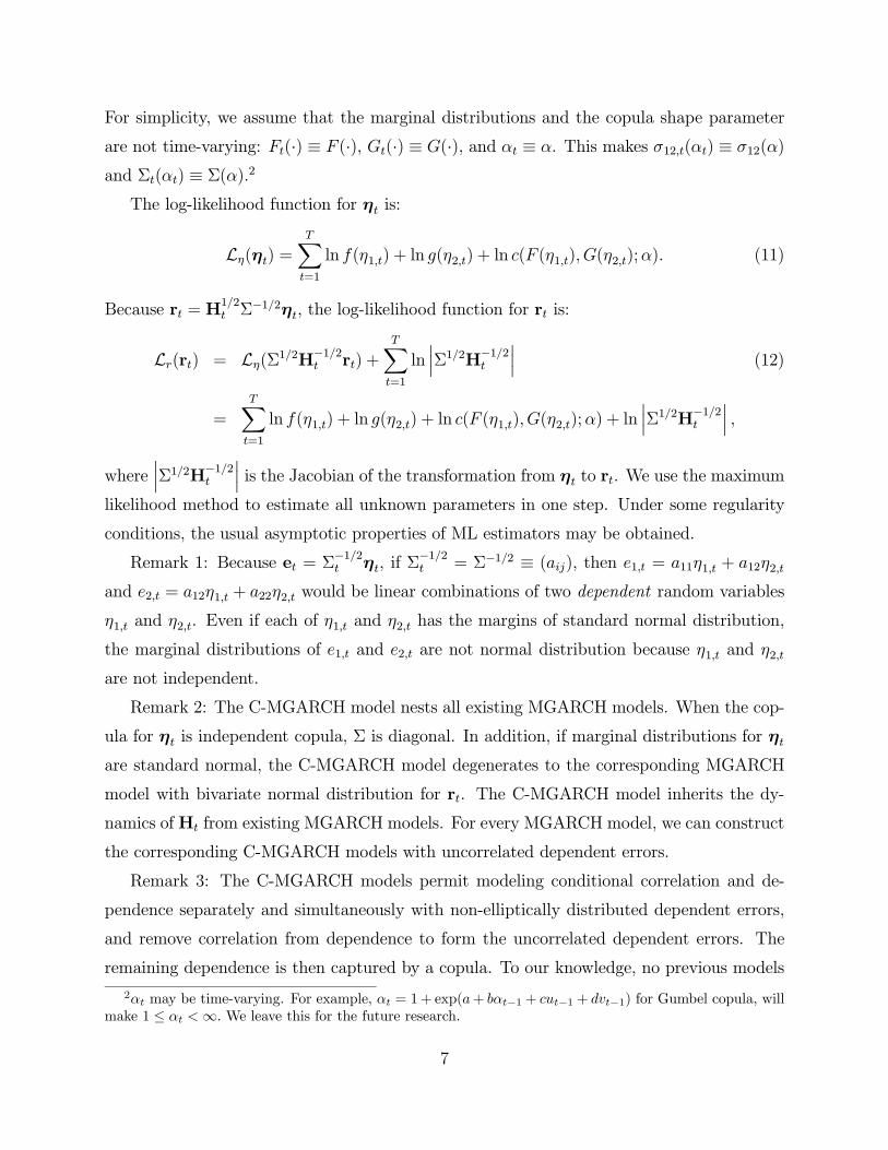
For simplicity, we assume that the marginal distributions and the copula shape parameter

are not time-varying: Ft(·) ≡ F (·), Gt(·) ≡ G(·), and αt ≡ α. This makes σ12,t(αt) ≡ σ12(α)

and Σt(αt) ≡ Σ(α).2

The log-likelihood function for ηt is:

Lη(ηt) =TXt=1

ln f(η1,t) + ln g(η2,t) + ln c(F (η1,t), G(η2,t);α). (11)

Because rt = H1/2t Σ−1/2ηt, the log-likelihood function for rt is:

Lr(rt) = Lη(Σ1/2H

−1/2t rt) +

TXt=1

ln¯Σ1/2H

−1/2t

¯(12)

=TXt=1

ln f(η1,t) + ln g(η2,t) + ln c(F (η1,t), G(η2,t);α) + ln¯Σ1/2H

−1/2t

¯,

where¯Σ1/2H

−1/2t

¯is the Jacobian of the transformation from ηt to rt. We use the maximum

likelihood method to estimate all unknown parameters in one step. Under some regularity

conditions, the usual asymptotic properties of ML estimators may be obtained.

Remark 1: Because et = Σ−1/2t ηt, if Σ

−1/2t = Σ−1/2 ≡ (aij), then e1,t = a11η1,t + a12η2,t

and e2,t = a12η1,t + a22η2,t would be linear combinations of two dependent random variables

η1,t and η2,t. Even if each of η1,t and η2,t has the margins of standard normal distribution,

the marginal distributions of e1,t and e2,t are not normal distribution because η1,t and η2,t

are not independent.

Remark 2: The C-MGARCH model nests all existing MGARCH models. When the cop-

ula for ηt is independent copula, Σ is diagonal. In addition, if marginal distributions for ηt

are standard normal, the C-MGARCH model degenerates to the corresponding MGARCH

model with bivariate normal distribution for rt. The C-MGARCH model inherits the dy-

namics ofHt from existing MGARCH models. For every MGARCH model, we can construct

the corresponding C-MGARCH models with uncorrelated dependent errors.

Remark 3: The C-MGARCH models permit modeling conditional correlation and de-

pendence separately and simultaneously with non-elliptically distributed dependent errors,

and remove correlation from dependence to form the uncorrelated dependent errors. The

remaining dependence is then captured by a copula. To our knowledge, no previous models

2αt may be time-varying. For example, αt = 1+ exp(a+ bαt−1 + cut−1 + dvt−1) for Gumbel copula, willmake 1 ≤ αt <∞. We leave this for the future research.

7

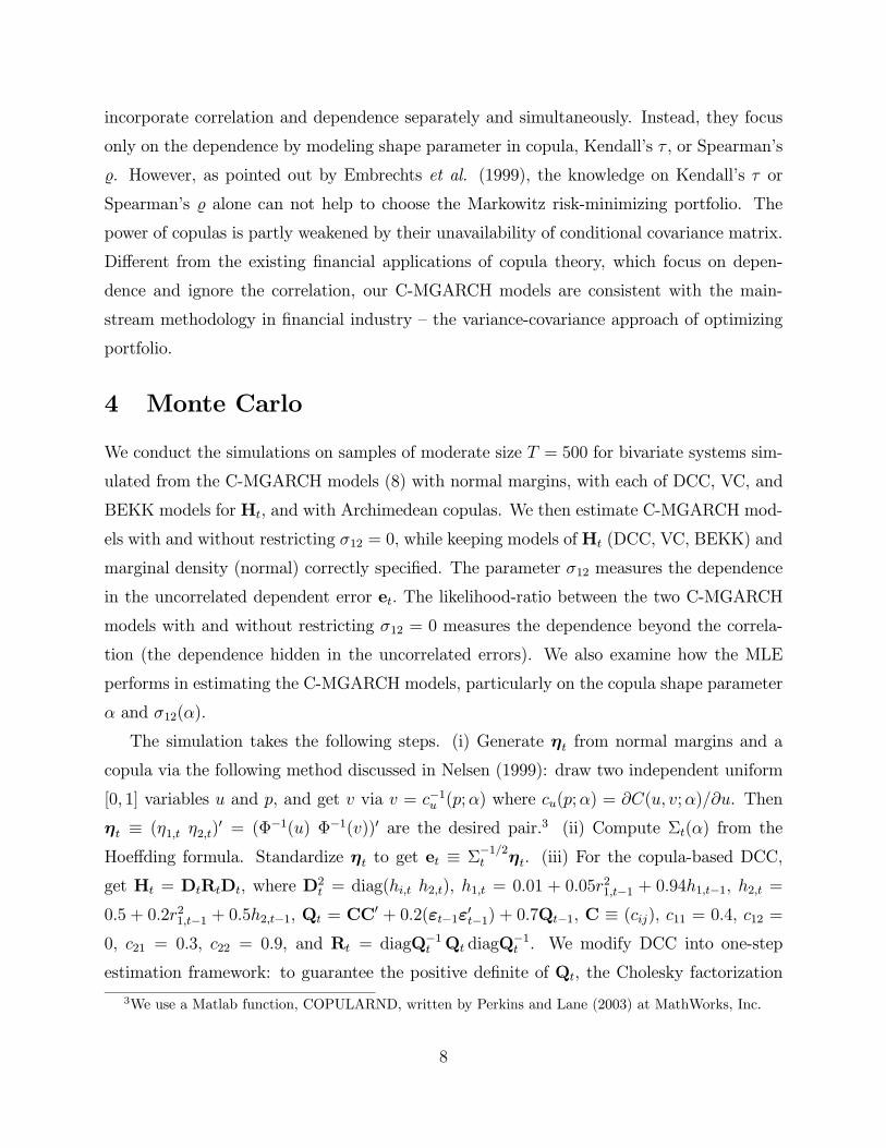
incorporate correlation and dependence separately and simultaneously. Instead, they focus

only on the dependence by modeling shape parameter in copula, Kendall’s τ , or Spearman’s

%. However, as pointed out by Embrechts et al. (1999), the knowledge on Kendall’s τ or

Spearman’s % alone can not help to choose the Markowitz risk-minimizing portfolio. The

power of copulas is partly weakened by their unavailability of conditional covariance matrix.

Different from the existing financial applications of copula theory, which focus on depen-

dence and ignore the correlation, our C-MGARCH models are consistent with the main-

stream methodology in financial industry — the variance-covariance approach of optimizing

portfolio.

4 Monte Carlo

We conduct the simulations on samples of moderate size T = 500 for bivariate systems sim-

ulated from the C-MGARCH models (8) with normal margins, with each of DCC, VC, and

BEKK models for Ht, and with Archimedean copulas. We then estimate C-MGARCH mod-

els with and without restricting σ12 = 0, while keeping models ofHt (DCC, VC, BEKK) and

marginal density (normal) correctly specified. The parameter σ12 measures the dependence

in the uncorrelated dependent error et. The likelihood-ratio between the two C-MGARCH

models with and without restricting σ12 = 0 measures the dependence beyond the correla-

tion (the dependence hidden in the uncorrelated errors). We also examine how the MLE

performs in estimating the C-MGARCH models, particularly on the copula shape parameter

α and σ12(α).

The simulation takes the following steps. (i) Generate ηt from normal margins and a

copula via the following method discussed in Nelsen (1999): draw two independent uniform

[0, 1] variables u and p, and get v via v = c−1u (p;α) where cu(p;α) = ∂C(u, v;α)/∂u. Then

ηt ≡ (η1,t η2,t)0 = (Φ−1(u) Φ−1(v))0 are the desired pair.3 (ii) Compute Σt(α) from the

Hoeffding formula. Standardize ηt to get et ≡ Σ−1/2t ηt. (iii) For the copula-based DCC,

get Ht = DtRtDt, where D2t = diag(hi,t h2,t), h1,t = 0.01 + 0.05r21,t−1 + 0.94h1,t−1, h2,t =

0.5 + 0.2r21,t−1 + 0.5h2,t−1, Qt = CC0 + 0.2(εt−1ε

0t−1) + 0.7Qt−1, C ≡ (cij), c11 = 0.4, c12 =

0, c21 = 0.3, c22 = 0.9, and Rt = diagQ−1t Qt diagQ−1t . We modify DCC into one-step

estimation framework: to guarantee the positive definite of Qt, the Cholesky factorization

3We use a Matlab function, COPULARND, written by Perkins and Lane (2003) at MathWorks, Inc.

8

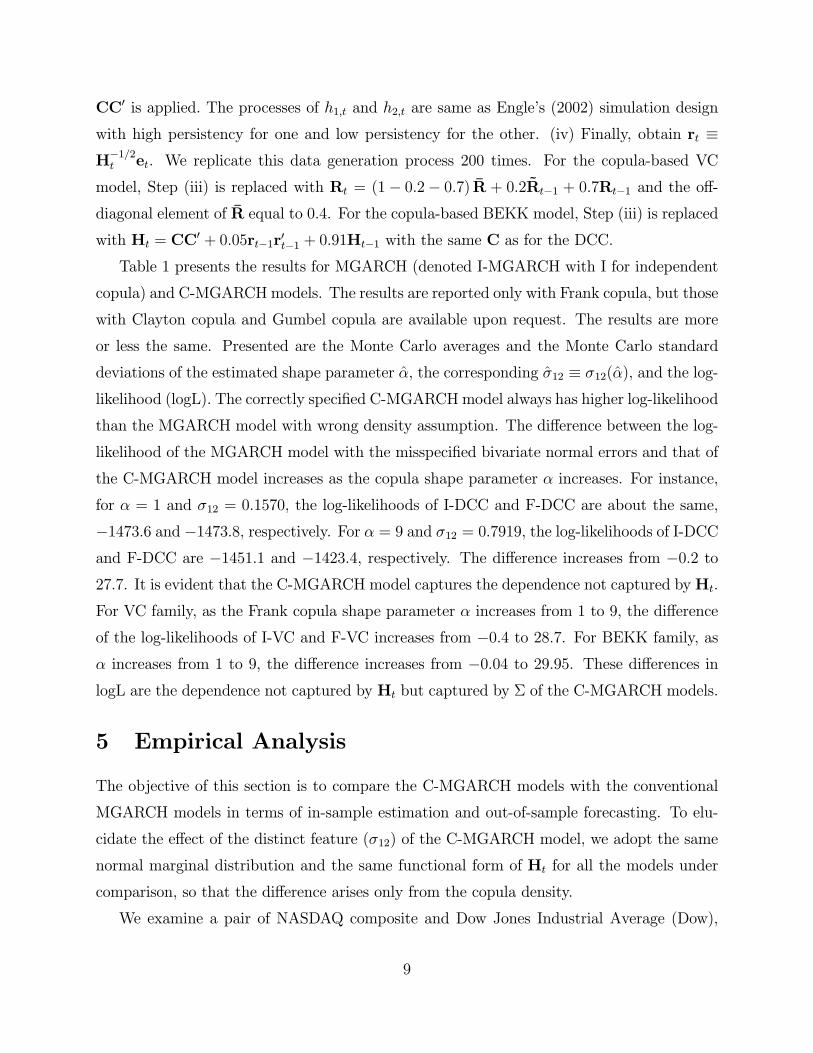
CC0 is applied. The processes of h1,t and h2,t are same as Engle’s (2002) simulation design

with high persistency for one and low persistency for the other. (iv) Finally, obtain rt ≡H−1/2t et. We replicate this data generation process 200 times. For the copula-based VC

model, Step (iii) is replaced with Rt = (1− 0.2− 0.7) R + 0.2Rt−1 + 0.7Rt−1 and the off-

diagonal element of R equal to 0.4. For the copula-based BEKK model, Step (iii) is replaced

with Ht = CC0 + 0.05rt−1r

0t−1 + 0.91Ht−1 with the same C as for the DCC.

Table 1 presents the results for MGARCH (denoted I-MGARCH with I for independent

copula) and C-MGARCHmodels. The results are reported only with Frank copula, but those

with Clayton copula and Gumbel copula are available upon request. The results are more

or less the same. Presented are the Monte Carlo averages and the Monte Carlo standard

deviations of the estimated shape parameter α, the corresponding σ12 ≡ σ12(α), and the log-

likelihood (logL). The correctly specified C-MGARCHmodel always has higher log-likelihood

than the MGARCH model with wrong density assumption. The difference between the log-

likelihood of the MGARCH model with the misspecified bivariate normal errors and that of

the C-MGARCH model increases as the copula shape parameter α increases. For instance,

for α = 1 and σ12 = 0.1570, the log-likelihoods of I-DCC and F-DCC are about the same,

−1473.6 and −1473.8, respectively. For α = 9 and σ12 = 0.7919, the log-likelihoods of I-DCCand F-DCC are −1451.1 and −1423.4, respectively. The difference increases from −0.2 to27.7. It is evident that the C-MGARCH model captures the dependence not captured byHt.

For VC family, as the Frank copula shape parameter α increases from 1 to 9, the difference

of the log-likelihoods of I-VC and F-VC increases from −0.4 to 28.7. For BEKK family, asα increases from 1 to 9, the difference increases from −0.04 to 29.95. These differences inlogL are the dependence not captured by Ht but captured by Σ of the C-MGARCH models.

5 Empirical Analysis

The objective of this section is to compare the C-MGARCH models with the conventional

MGARCH models in terms of in-sample estimation and out-of-sample forecasting. To elu-

cidate the effect of the distinct feature (σ12) of the C-MGARCH model, we adopt the same

normal marginal distribution and the same functional form of Ht for all the models under

comparison, so that the difference arises only from the copula density.

We examine a pair of NASDAQ composite and Dow Jones Industrial Average (Dow),

9

and two pairs of foreign exchange (FX) rate series (in U.S. dollars) — French Franc (FF)

and Deutschemark (DM), and Japanese Yen (JY) and Deutschemark. The return series are

100 times the log difference of the stock indices or exchange rates. The daily U.S. equity

indices are obtained from finance.yahoo.com, and the daily spot FX series are from the

Federal Reserve Statistical Release. The sample periods of the data, out-of-sample forecast

validation periods, and the size of rolling window to train forecasting models are as follows:

In-sample estimation Out-of-sample forecastingNASDAQ-DOW Jan. 2, 1997 to Dec. 31, 2001 Jan. 4, 2001 to Dec. 31, 2001

T = 1257 P = 248 with rolling window R = 1009FF-DM Jan. 4, 1993 to Dec. 31, 1998 Jan. 7, 1997 to Dec. 31, 1998

T = 1509 P = 500 with rolling window R = 1009JY-DM Jan. 4, 1993 to Dec. 31, 1997 Jan. 5, 1997 to Dec. 31, 1997

T = 1257 P = 250 with rolling window R = 1007

5.1 In-sample estimation

For the in-sample comparison between our C-MGARCH models and MGARCH models,

Table 2 presents three model selection criteria (likelihood, AIC, SIC). For the NASDAQ-

DOW pair and for the FF-DM pair, Gumbel Survival copula or Joe-Clayton copula are

selected. Joe-Clayton copula nests Clayton copula as a special case. Gumbel Survival

copula, Joe-Clayton copula, and Clayton copula all have the asymmetric tail dependence

with positive lower tail dependence (λL > 0) and zero upper tail dependence (λU = 0). This

characteristic implies so called “crashing-together”. For the JY-DM pair, the model selection

criteria select Frank copula, which has symmetric tail dependence. The log-likelihood ratio

of two models is the entropy gain in the sense of Vuong (1989). The superiority of Gumbel

Survival copula and Joe-Clayton copula (for NASDAQ-DOW and FF-DM) and Frank copula

(for JY-DM) over the independent copula (i.e., multivariate normal distribution) indicates

that the conditional joint distributions of these three pairs of equity and FX return series

are not bivariate normal.

Table 2 also presents the estimated shape parameters α, their robust standard errors, and

the corresponding σ12. For FF-DM, the estimated shape parameters for the Gumbel Survival

copula and Joe-Clayton copula are very significant. For JY-DM, the estimated shape pa-

rameter of Frank copula is 8.44 in Frank-DCC, 8.38 in Frank-VC and 6.98 in Frank-BEKK,

10

and all significantly positive, indicating the remaining dependence in the standardized un-

correlated errors et is strong, positive, and symmetric in both tails.

5.2 Out-of-sample predictive ability

Suppose there are l + 1 models in a set of the competing density forecast models, possibly

misspecified. We compare l = 6 C-MGARCH models with the benchmark MGARCH model.

Let these models be indexed by j (j = 0, 1, . . . , l = 6) with the jth density forecast model

denoted by ψjt(rt; θj

R,t−1). The benchmark model is indexed with j = 0. If a bivariate density

forecast model ψt(rt;θ0) coincides with the true density ϕt(rt) almost surely for some θ0∈ Θ,

then the one-step-ahead density forecast is said to be optimal because it dominates all other

density forecasts for any loss functions (Diebold et al., 1998; Granger and Pesaran, 2000). As

in practice it is rarely the case that we can find an optimal model, our task is to investigate

which density forecast model approximates the true conditional density most closely. If a

metric is defined to measure the distance of a given model to the truth, we then compare

different models in terms of this distance.

Following Bao et al. (2005), we compare C-MGARCH models by comparing the condi-

tional Kullback-Leibler information criterion (KLIC), It¡ϕ : ψj,θ

¢= Eϕt ln[ϕt (yt) /ψ

jt

¡yt;θ

j¢],

where the expectation is with respect to the true conditional density ϕt (·|Ft−1). Fol-

lowing White (1994), we define the distance between a density model and the true den-

sity as the minimum KLIC, It(ϕ : ψj,θ∗jt−1) = Eϕt ln[ϕt (yt) /ψjt(yt;θ

∗jt−1)], where θ

∗jt−1 =

argmin It¡ϕ : ψj,θj

¢is the pseudo-true value of θj. To estimate θ∗jt−1, we split the data

into two parts — one for the estimation and the other for out-of-sample validation. At each

period t in the out-of-sample period (t = R + 1, . . . , T ), we use the previous R rolling ob-

servations {yt−1, . . . , yt−R}Tt=R+1 to estimate the unknown parameter vector θ∗jt−1 and denote

the estimate as θj

R,t−1.4 Under some regularity conditions, we can consistently estimate

θ∗jt−1 by θj

R,t−1 by maximizing R−1Pt

s=t−R+1 lnψjs

¡ys;θ

j¢. See White (1994) for the sets of

conditions for the existence and consistency of θj

R,t−1.

Using {θR,t−1}Tt=R+1, we can obtain the out-of-sample estimate of EIt(ϕ : ψj,θ∗jt−1) by

IR,n(ϕ : ψ) ≡ P−1PT

t=R+1 ln[ϕt(yt)/ψjt(yt; θ

j

R,t−1)], where P ≡ T − R is the size of the out-of-sample period. Since the KLIC takes a smaller value when a model is closer to the truth,

4Alternatively, θ∗t−1 can be estimated based on the whole subsample {yt−1, . . . , y1} or a fixed sample{yR, . . . , y1}.

11

we can regard it as a loss function. Bao et al. (2005) note that the out-of-sample average of

the KLIC-differential between the benchmark model 0 and model j is then simply the log

ratio of the predictive likelihoods

IR,n(ϕ : ψ0)− IR,n(ϕ : ψj) =1

P

TXt=R+1

ln[ψjt(yt; θj

R,t−1)/ψ0t (yt; θ

0

R,t−1)]. (13)

When we compare multiple l C-MGARCH models using various copulas against a benchmark

MGARCH model, the null hypothesis of interest is that no C-MGARCH model is better

than the benchmark MGARCH. White (2000) proposes a test statistic and the bootstrap

procedure to compute its p-value.

Table 3 reports the density forecast comparison in terms of the out-of-sample KLIC

together with the reality check p-values. In general, the in-sample results in Table 2 and

the out-of-sample results in Table 3 are consistent, in that the in-sample ranking across the

C-MGARCH models is carried over to the out-of-sample predictive ranking of the models.

For NASDAQ-DOW and for FF-DM, the density forecast comparison confirms the non-

normality. For all three families (DCC, VC, BEKK), the independent copula yields the

smallest (worst) predictive likelihood among all seven C-MGARCH models. The predictive

superiority of C-MGARCH models based on Gumbel Survival copula or Joe-Clayton copula

over the MGARCH model based on the independent copula (MGARCH under the bivariate

normal distribution) is marginally significant for NASDAQ-DOW (with the reality check

p-values 0.087, 0.095, 0.195, respectively for DCC, VC, BEKK families) and is strongly

significant for FF-DM (with the reality check p-values 0.002, 0.000, 0.008 respectively for

DCC, VC, BEKK families). For these two pairs of return series, Gumbel Survival or Joe-

Clayton C-MGARCH is significantly better than the benchmark even after accounting for

potential bias due to the specification search.

For JY-DM, the independent copula yields one of the worst predictive likelihood. The

largest (best) predictive likelihood is obtained from the Frank C-MGARCH for all three

families. The result for JY-DM is weaker than for FF-DM, as the reality check p-values

are 0.184, 0.144, 0.181, respectively for DCC, VC, BEKK families. This result is consistent

with the results of Chen and Fan (2005, Section 6.1), who find much stronger rejection of

normality for FF-DM than for JY-DM. They also find much stronger tail dependence for

FF-DM than for JY-DM.

12

6 Conclusions

In this paper we propose a new MGARCH model, namely, the C-MGARCH model. The

C-MGARCH model includes a conventional MGARCH model as a special case. The C-

MGARCH model is to exploit the fact that the uncorrelated errors are not necessarily in-

dependent. The C-MGARCH model permits modeling the conditional covariance for the

non-elliptically distributed financial returns, and at the same time separately modeling the

dependence structure beyond the conditional covariance. While we have considered here

only a bivariate system, the extension to a higher dimension is straightforward. We compare

the C-MGARCH models with the corresponding MGARCH models using the three financial

data sets — a pair of the U.S. equity indices and two pairs of the foreign exchange rates.

The empirical results from the in-sample and out-of-sample analysis clearly demonstrate the

advantages of the new model.

7 Appendix

We present here some details on copula functions for two widely used copula families —

elliptical copula family and Archimedean copula family. The former includes the Gaussian

copula and the Student’s t copula. The later includes Gumbel copula, Clayton copula and

Frank copula. We also discuss the survival copulas of Archimedean copulas and Joe-Clayton

copula.

7.1 Elliptical copulas

Gaussian copula: Let R be the symmetric, positive definite correlation matrix and ΦR(·, ·)be the standard bivariate normal distribution with correlation matrix R. The density func-

tion of bivariate Gaussian copula is:

cGaussian(u, v) =1

|R|1/2 exp(−1

2η0(R−1−I)η), (14)

where η = (Φ−1(u) Φ−1(v))0 and Φ−1(·) is the inverse of the univariate normal CDF. Thebivariate Gaussian copula is:

CGaussian(u, v;R) = ΦR¡Φ−1(u),Φ−1(v)

¢.

13

Hu (2003) shows the bivariate Gaussian copula can be approximated by Taylor expansion:

CGaussian(u, v; ρ) ≈ uv + ρφ(Φ−1(u))φ(Φ−1(v)),

where φ is the density function of univariate Gaussian distribution and ρ is the correla-

tion coefficient between η1 and η2. Both the upper tail dependence λU and the lower tail

dependence λL are zero, reflecting the asymptotic tail independence of Gaussian copula.

Student’s t copula: Let ωc be the degree of freedom, and TR,ωc(·, ·) be the standardbivariate Student’s t distribution with degree of freedom ωc and correlation matrix R. The

density function of bivariate Student’s t copula is:

cStudent’s t(u, v;R,ωc) = |R|−

12Γ(ωc+2

2)Γ(ωc

2)

Γ(ωc+12)2

(1 + η0R−1ηωc

)−ωc+22

Π2i=1(1 +η2iωc)−

ωc+12

where η = (t−1ωc (u), t−1ωc (v))

0, u = tω1(x), v = tω2(y), and tωi(·) is the univariate Student’s tCDF with degree of freedom ωi. The bivariate Student’s t copula is

CStudent’s t(u, v;R,ωc) = TR,ωc

¡t−1ωc (u), t

−1ωc (v)

¢.

The upper tail dependence λU of Student’s t copula is λU = 2−2tωc+1¡√

ωc + 1√1− ρ/

√1 + ρ

¢,

where ρ is the off-diagonal element of R. Because of the symmetry property, the lower tail

dependence λL can be obtained easily.

7.2 Archimedean copulas

Archimedean copula can be expressed as

C(u, v) = ϕ−1(ϕ(u) + ϕ(v)),

where ϕ is a convex decreasing function, called generator. Different generator will induce

different copula in the family of Archimedean copula. The Kendall’s τ = 1 + 4

Z 1

0

ϕ(u)ϕ0(u)du.

Gumbel copula: The generator for Gumbel copula is ϕα(x) = (− lnx)α. For 1 ≤ α <∞(α = 1 for independence and α→∞ for more dependence), the CDF and PDF for Gumbel

copula are

CGumbel(u, v;α) = exp{−[(− lnu)α + (− ln v)α]1/α},

cGumbel(u, v;α) =CGumbel(u, v;α)(lnu ln v)α−1{[(− lnu)α + (− ln v)α]1/α + α− 1}

uv[(− lnu)α + (− ln v)α]2−1/α .

14

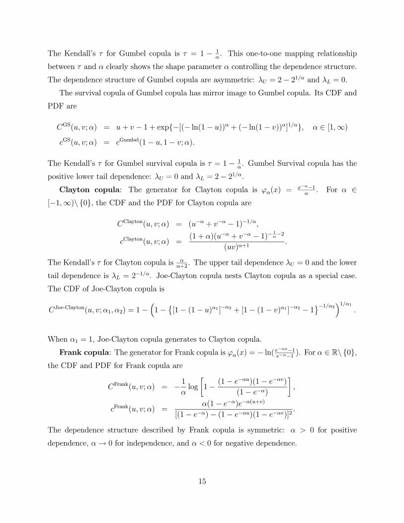
The Kendall’s τ for Gumbel copula is τ = 1 − 1α. This one-to-one mapping relationship

between τ and α clearly shows the shape parameter α controlling the dependence structure.

The dependence structure of Gumbel copula are asymmetric: λU = 2− 21/α and λL = 0.

The survival copula of Gumbel copula has mirror image to Gumbel copula. Its CDF and

PDF are

CGS(u, v;α) = u+ v − 1 + exp{−[(− ln(1− u))α + (− ln(1− v))α]1/α}, α ∈ [1,∞)

cGS(u, v;α) = cGumbel(1− u, 1− v;α).

The Kendall’s τ for Gumbel survival copula is τ = 1− 1α. Gumbel Survival copula has the

positive lower tail dependence: λU = 0 and λL = 2− 21/α.Clayton copula: The generator for Clayton copula is ϕα(x) =

x−α−1α. For α ∈

[−1,∞)\ {0}, the CDF and the PDF for Clayton copula are

CClayton(u, v;α) = (u−α + v−α − 1)−1/α,

cClayton(u, v;α) =(1 + α)(u−α + v−α − 1)− 1

α−2

(uv)α+1.

The Kendall’s τ for Clayton copula is αα+2. The upper tail dependence λU = 0 and the lower

tail dependence is λL = 2−1/α. Joe-Clayton copula nests Clayton copula as a special case.

The CDF of Joe-Clayton copula is

CJoe-Clayton(u, v;α1,α2) = 1−³1−

©[1− (1− u)α1]−α2 + [1− (1− v)α1 ]−α2 − 1

ª−1/α2´1/α1.

When α1 = 1, Joe-Clayton copula generates to Clayton copula.

Frank copula: The generator for Frank copula is ϕα(x) = − ln(e−αx−1e−α−1 ). For α ∈ R\ {0},

the CDF and PDF for Frank copula are

CFrank(u, v;α) = − 1αlog

∙1− (1− e

−αu)(1− e−αv)(1− e−α)

¸,

cFrank(u, v;α) =α(1− e−α)e−α(u+v)

[(1− e−α)− (1− e−αu)(1− e−αv)]2 .

The dependence structure described by Frank copula is symmetric: α > 0 for positive

dependence, α→ 0 for independence, and α < 0 for negative dependence.

15

References

Bao, Y., T.-H. Lee, and B. Saltoglu (2005), “Comparing Density Forecast Models”, UCR.

Breymann, W., A. Dias, P. Embrechts (2003), “Dependence Structures for MultivariateHigh-Frequency Data in Finance”, Quantitative Finance 3, 1-16.

Chen, X. and Y. Fan (2005), “Estimation and Model Selection of Semiparametric Copula-Based Multivariate Dynamic Models under Copula Misspecification”, Journal of Econo-metrics, forthcoming.

Diebold, F.X., T.A. Gunther, and A. S. Tay (1998), “Evaluating Density Forecasts withApplications to Financial Risk Management”, International Economic Review 39, 863-883.

Embrechts, P., A. McNeil, and D. Straumann (1999), “Correlation: Pitfalls and Alterna-tives”, ETH Zentrum.

Engle, R.F. (2002), “Dynamic Conditional Correlation: A Simple Class of MultivariateGeneralized Autoregressive Conditional Heteroskedasticity Models”, Journal of Busi-ness and Economic Statistics 20, 339-350.

Engle, R.F. and K.F. Kroner (1995), “Multivariate Simultaneous Generalized ARCH”,Econometric Theory 11, 122-50.

Fama, E. and K. French (1993), Common Risk Factors in the Returns on Stocks and Bonds,Journal of Financial Economics 33, 3—56.

Granger, C.W.J. and M.H. Pesaran (2000), “Economic and Statistical Measures of ForecastAccuracy,” Journal of Forecasting 19, 537-560.

Hansen, P.R. (2001), “An Unbiased and Powerful for Superior Predictive Ability”, Stanford.

Hoeffding, W. (1940), Masstabinvariante Korrelationstheorie, Schriten des MatematischenInstituts und des Instituts fur angewandte Mathematik der Universitat Berlin, 5, Heft3, 179-233. [Reprinted as Scale-invariant correlation theory in The Collected Worksof Wassily Hoeffding, N.I. fisher and P.K. Sen editors, Springer-Verlag, New York,57-107].

Hu, L. (2003), “Dependence Patterns across Financial Markets: a Mixed Copula Approach”,OSU.

Lehmann, E.L. (1966), “Some Concepts of Dependence”, Annals of Mathematical Statistics37, 1137-1153.

Longin, F. and B. Solnik (2001), “Extreme Correlation of International Equity Market”,Journal of Finance 56, 649-679.

Mashal, R. and A. Zeevi (2002), “Beyond Correlation: Extreme Co-movements Betweenfinancial Assets”, Columbia University.

Nelsen, R.B. (1999), An Introduction to Copulas, Springer-Verlag, New York.

Perkins, P. and T. Lane (2003), “Monte-Carlo Simulation in MATLAB Using Copulas”,MATLAB News & Notes, November 2003.

16

Richardson, M.P. and T. Smith (1993), “A Test of Multivariate Normality of Stock Re-turns”, Journal of Business 66, 295-321.

Shea, G.A. (1983), “Hoeffding’s Lemma”, Encyclopedia of Statistical Sciences, Vol. 3, S.Kotz and N.L. Johnson (editors), John Wiley & Sons, New York, 648-649.

Sklar, A. (1959), “Fonctions de repartition a n dimensions et leurs marges”, Publicationsde Institut Statistique de Universite de Paris 8, 229—231.

Tse, Y.K. and A.K. Tsui (2002), “A Multivariate Generalized Autoregressive ConditionalHeteroscedasticity Model with Time-Varying Correlations”, Journal of Business andEconomic Statistics 20, 351-362.

Vuong, Q. (1989), “Likelihood Ratio Tests for Model Selection and Non-nested Hypothe-ses”, Econometrica 57, 307-333.

White, H. (1994), Estimation, Inference, and Specification Analysis. Cambridge UniversityPress.

White, H. (2000), “A Reality Check for Data Snooping”, Econometrica 68, 1097-1126.

17

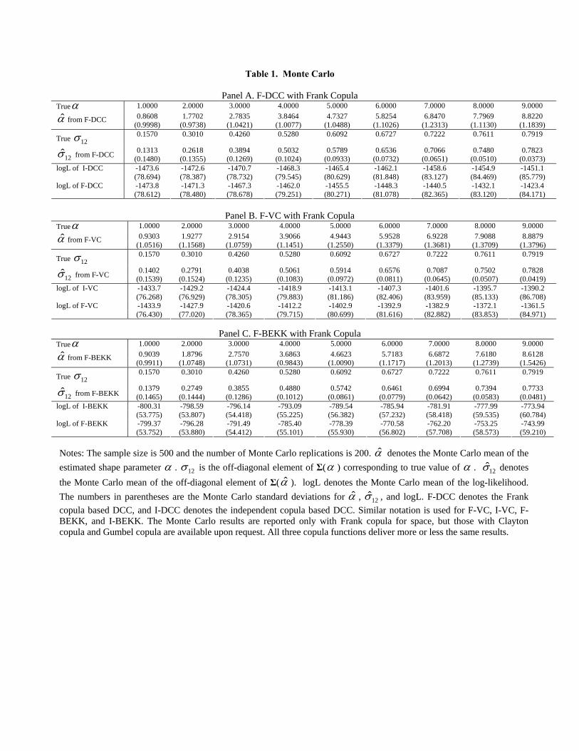
Table 1. Monte Carlo

Panel A. F-DCC with Frank Copula Trueα 1.0000 2.0000 3.0000 4.0000 5.0000 6.0000 7.0000 8.0000 9.0000

0.8608 1.7702 2.7835 3.8464 4.7327 5.8254 6.8470 7.7969 8.8220 α from F-DCC (0.9998) (0.9738) (1.0421) (1.0077) (1.0488) (1.1026) (1.2313) (1.1130) (1.1839)

True 12σ 0.1570 0.3010 0.4260 0.5280 0.6092 0.6727 0.7222 0.7611 0.7919

0.1313 0.2618 0.3894 0.5032 0.5789 0.6536 0.7066 0.7480 0.7823 12σ from F-DCC (0.1480) (0.1355) (0.1269) (0.1024) (0.0933) (0.0732) (0.0651) (0.0510) (0.0373)

-1473.6 -1472.6 -1470.7 -1468.3 -1465.4 -1462.1 -1458.6 -1454.9 -1451.1 logL of I-DCC (78.694) (78.387) (78.732) (79.545) (80.629) (81.848) (83.127) (84.469) (85.779) -1473.8 -1471.3 -1467.3 -1462.0 -1455.5 -1448.3 -1440.5 -1432.1 -1423.4 logL of F-DCC (78.612) (78.480) (78.678) (79.251) (80.271) (81.078) (82.365) (83.120) (84.171)

Panel B. F-VC with Frank Copula

Trueα 1.0000 2.0000 3.0000 4.0000 5.0000 6.0000 7.0000 8.0000 9.0000 0.9303 1.9277 2.9154 3.9066 4.9443 5.9528 6.9228 7.9088 8.8879 α from F-VC

(1.0516) (1.1568) (1.0759) (1.1451) (1.2550) (1.3379) (1.3681) (1.3709) (1.3796)

True 12σ 0.1570 0.3010 0.4260 0.5280 0.6092 0.6727 0.7222 0.7611 0.7919

0.1402 0.2791 0.4038 0.5061 0.5914 0.6576 0.7087 0.7502 0.7828 12σ from F-VC (0.1539) (0.1524) (0.1235) (0.1083) (0.0972) (0.0811) (0.0645) (0.0507) (0.0419)

-1433.7 -1429.2 -1424.4 -1418.9 -1413.1 -1407.3 -1401.6 -1395.7 -1390.2 logL of I-VC (76.268) (76.929) (78.305) (79.883) (81.186) (82.406) (83.959) (85.133) (86.708) -1433.9 -1427.9 -1420.6 -1412.2 -1402.9 -1392.9 -1382.9 -1372.1 -1361.5 logL of F-VC (76.430) (77.020) (78.365) (79.715) (80.699) (81.616) (82.882) (83.853) (84.971)

Panel C. F-BEKK with Frank Copula

Trueα 1.0000 2.0000 3.0000 4.0000 5.0000 6.0000 7.0000 8.0000 9.0000 0.9039 1.8796 2.7570 3.6863 4.6623 5.7183 6.6872 7.6180 8.6128 α from F-BEKK

(0.9911) (1.0748) (1.0731) (0.9843) (1.0090) (1.1717) (1.2013) (1.2739) (1.5426)

True 12σ 0.1570 0.3010 0.4260 0.5280 0.6092 0.6727 0.7222 0.7611 0.7919

0.1379 0.2749 0.3855 0.4880 0.5742 0.6461 0.6994 0.7394 0.7733 12σ from F-BEKK (0.1465) (0.1444) (0.1286) (0.1012) (0.0861) (0.0779) (0.0642) (0.0583) (0.0481)

-800.31 -798.59 -796.14 -793.09 -789.54 -785.94 -781.91 -777.99 -773.94 logL of I-BEKK (53.775) (53.807) (54.418) (55.225) (56.382) (57.232) (58.418) (59.535) (60.784) -799.37 -796.28 -791.49 -785.40 -778.39 -770.58 -762.20 -753.25 -743.99 logL of F-BEKK (53.752) (53.880) (54.412) (55.101) (55.930) (56.802) (57.708) (58.573) (59.210)

Notes: The sample size is 500 and the number of Monte Carlo replications is 200. α denotes the Monte Carlo mean of the estimated shape parameter α . 12σ is the off-diagonal element of Σ(α ) corresponding to true value of α . 12σ denotes the Monte Carlo mean of the off-diagonal element of Σ(α ). logL denotes the Monte Carlo mean of the log-likelihood. The numbers in parentheses are the Monte Carlo standard deviations for α , 12σ , and logL. F-DCC denotes the Frank copula based DCC, and I-DCC denotes the independent copula based DCC. Similar notation is used for F-VC, I-VC, F-BEKK, and I-BEKK. The Monte Carlo results are reported only with Frank copula for space, but those with Clayton copula and Gumbel copula are available upon request. All three copula functions deliver more or less the same results.

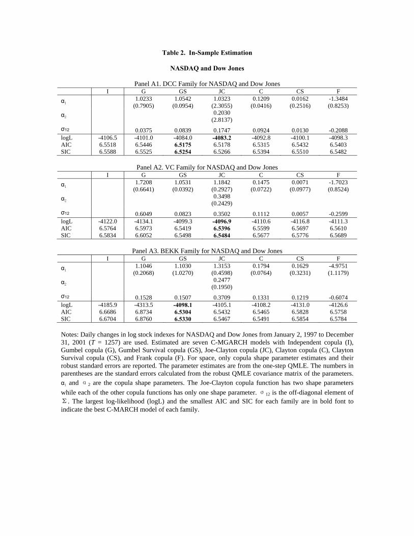
Table 2. In-Sample Estimation

NASDAQ and Dow Jones

Panel A1. DCC Family for NASDAQ and Dow Jones I G GS JC C CS F α1 1.0233

(0.7905) 1.0542

(0.0954) 1.0323

(2.3055) 0.1209

(0.0416) 0.0162

(0.2516) -1.3484 (0.8253)

α2

0.2030 (2.8137)

σ12 0.0375 0.0839 0.1747 0.0924 0.0130 -0.2088 logL -4106.5 -4101.0 -4084.0 -4083.2 -4092.8 -4100.1 -4098.3 AIC 6.5518 6.5446 6.5175 6.5178 6.5315 6.5432 6.5403 SIC 6.5588 6.5525 6.5254 6.5266 6.5394 6.5510 6.5482

Panel A2. VC Family for NASDAQ and Dow Jones

I G GS JC C CS F α1 1.7208

(0.6641) 1.0531

(0.0392) 1.1842

(0.2927) 0.1475

(0.0722) 0.0071

(0.0977) -1.7023 (0.8524)

α2

0.3498 (0.2429)

σ12 0.6049 0.0823 0.3502 0.1112 0.0057 -0.2599 logL -4122.0 -4134.1 -4099.3 -4096.9 -4110.6 -4116.8 -4111.3 AIC 6.5764 6.5973 6.5419 6.5396 6.5599 6.5697 6.5610 SIC 6.5834 6.6052 6.5498 6.5484 6.5677 6.5776 6.5689

Panel A3. BEKK Family for NASDAQ and Dow Jones

I G GS JC C CS F α1 1.1046

(0.2068) 1.1030

(1.0270) 1.3153

(0.4598) 0.1794

(0.0764) 0.1629

(0.3231) -4.9751 (1.1179)

α2

0.2477 (0.1950)

σ12 0.1528 0.1507 0.3709 0.1331 0.1219 -0.6074 logL -4185.9 -4313.5 -4098.1 -4105.1 -4108.2 -4131.0 -4126.6 AIC 6.6686 6.8734 6.5304 6.5432 6.5465 6.5828 6.5758 SIC 6.6704 6.8760 6.5330 6.5467 6.5491 6.5854 6.5784

Notes: Daily changes in log stock indexes for NASDAQ and Dow Jones from January 2, 1997 to December 31, 2001 (T = 1257) are used. Estimated are seven C-MGARCH models with Independent copula (I), Gumbel copula (G), Gumbel Survival copula (GS), Joe-Clayton copula (JC), Clayton copula (C), Clayton Survival copula (CS), and Frank copula (F). For space, only copula shape parameter estimates and their robust standard errors are reported. The parameter estimates are from the one-step QMLE. The numbers in parentheses are the standard errors calculated from the robust QMLE covariance matrix of the parameters. α1 and α2 are the copula shape parameters. The Joe-Clayton copula function has two shape parameters while each of the other copula functions has only one shape parameter. σ12 is the off-diagonal element of Σ. The largest log-likelihood (logL) and the smallest AIC and SIC for each family are in bold font to indicate the best C-MARCH model of each family.

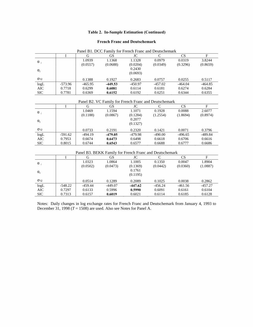
Table 2. In-Sample Estimation (Continued)

French Franc and Deutschemark

Panel B1. DCC Family for French Franc and Deutschemark I G GS JC C CS F α 1 1.0939

(0.0557) 1.1368

(0.0688) 1.1328

(0.0204) 0.0979

(0.0349) 0.0319

(0.3296) 3.8244

(0.8659) α2

0.2430

(0.0693) σ12 0.1388 0.1927 0.2683 0.0757 0.0255 0.5117 logL -573.96 -465.95 -449.53 -450.97 -457.02 -464.04 -464.85 AIC 0.7718 0.6299 0.6081 0.6114 0.6181 0.6274 0.6284 SIC 0.7781 0.6369 0.6152 0.6192 0.6251 0.6344 0.6355

Panel B2. VC Family for French Franc and Deutschemark

I G GS JC C CS F α 1 1.0469

(0.1188) 1.1594

(0.0867) 1.1071

(0.1284) 0.1928

(1.2554) 0.0088

(1.8694) 2.6077

(0.8974) α2

0.2077

(0.1327) σ12 0.0733 0.2191 0.2320 0.1421 0.0071 0.3796 logL -591.62 -494.19 -479.05 -479.98 -490.00 -496.65 -489.84 AIC 0.7953 0.6674 0.6473 0.6498 0.6618 0.6706 0.6616 SIC 0.8015 0.6744 0.6543 0.6577 0.6688 0.6777 0.6686

Panel B3. BEKK Family for French Franc and Deutschemark

I G GS JC C CS F α 1 1.0323

(0.0502) 1.0864

(0.0473) 1.1005

(0.1369) 0.1350

(0.0442) 0.0047

(0.0360) 1.8904

(1.0887) α2

0.1761

(0.1195) σ12 0.0514 0.1289 0.2089 0.1025 0.0038 0.2862 logL -548.22 -459.44 -449.07 -447.62 -456.24 -461.56 -457.27 AIC 0.7297 0.6133 0.5996 0.5990 0.6091 0.6161 0.6104 SIC 0.7313 0.6157 0.6019 0.6021 0.6114 0.6185 0.6128

Notes: Daily changes in log exchange rates for French Franc and Deutschemark from January 4, 1993 to December 31, 1998 (T = 1508) are used. Also see Notes for Panel A.

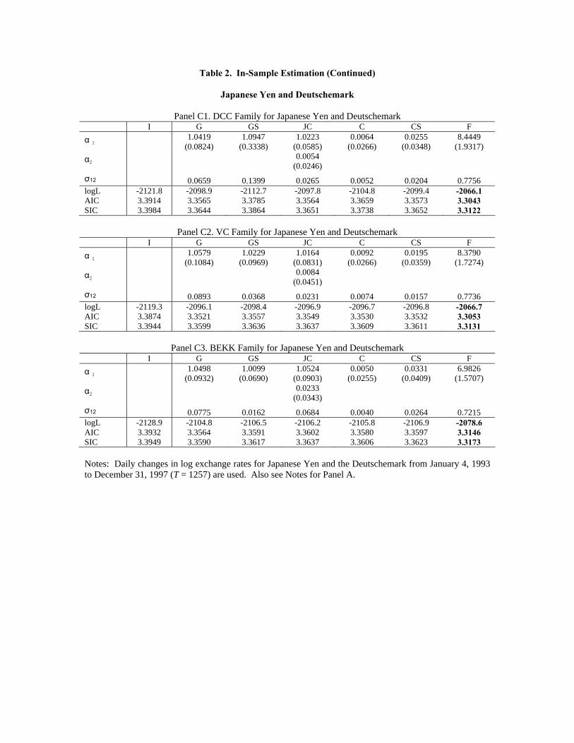
Table 2. In-Sample Estimation (Continued)

Japanese Yen and Deutschemark

Panel C1. DCC Family for Japanese Yen and Deutschemark I G GS JC C CS F α 1 1.0419

(0.0824) 1.0947

(0.3338) 1.0223

(0.0585) 0.0064

(0.0266) 0.0255

(0.0348) 8.4449

(1.9317) α2

0.0054

(0.0246) σ12 0.0659 0.1399 0.0265 0.0052 0.0204 0.7756 logL -2121.8 -2098.9 -2112.7 -2097.8 -2104.8 -2099.4 -2066.1 AIC 3.3914 3.3565 3.3785 3.3564 3.3659 3.3573 3.3043 SIC 3.3984 3.3644 3.3864 3.3651 3.3738 3.3652 3.3122

Panel C2. VC Family for Japanese Yen and Deutschemark

I G GS JC C CS F α 1 1.0579

(0.1084) 1.0229

(0.0969) 1.0164

(0.0831) 0.0092

(0.0266) 0.0195

(0.0359) 8.3790

(1.7274) α2

0.0084

(0.0451) σ12 0.0893 0.0368 0.0231 0.0074 0.0157 0.7736 logL -2119.3 -2096.1 -2098.4 -2096.9 -2096.7 -2096.8 -2066.7 AIC 3.3874 3.3521 3.3557 3.3549 3.3530 3.3532 3.3053 SIC 3.3944 3.3599 3.3636 3.3637 3.3609 3.3611 3.3131

Panel C3. BEKK Family for Japanese Yen and Deutschemark

I G GS JC C CS F α 1 1.0498

(0.0932) 1.0099

(0.0690) 1.0524

(0.0903) 0.0050

(0.0255) 0.0331

(0.0409) 6.9826

(1.5707) α2

0.0233

(0.0343) σ12 0.0775 0.0162 0.0684 0.0040 0.0264 0.7215 logL -2128.9 -2104.8 -2106.5 -2106.2 -2105.8 -2106.9 -2078.6 AIC 3.3932 3.3564 3.3591 3.3602 3.3580 3.3597 3.3146 SIC 3.3949 3.3590 3.3617 3.3637 3.3606 3.3623 3.3173

Notes: Daily changes in log exchange rates for Japanese Yen and the Deutschemark from January 4, 1993 to December 31, 1997 (T = 1257) are used. Also see Notes for Panel A.

Table 3. Out-of-Sample Predictive Ability

NASDAQ and Dow Jones

French Franc and Deutschemark

Japanese Yen and Deutschemark

Copula DCC VC BEKK DCC VC BEKK DCC VC BEKK I -3.5904 -3.5957 -3.5941 0.0604 -0.0731 0.0725 -1.9418 -1.9452 -1.9356 G -3.5663 -3.5770 -3.5757 0.1029 -0.0330 0.0893 -1.9425 -1.9448 -1.9322 GS -3.5603 -3.5712 -3.5721 0.1022 -0.0068 0.0889 -1.9412 -1.9432 -1.9388 JC -3.5661 -3.5671 -3.5677 0.1114 -0.0018 0.1048 -1.9403 -1.9393 -1.9382 C -3.5737 -3.5797 -3.5700 0.0927 -0.0309 0.0895 -1.9455 -1.9458 -1.9391 CS -3.5683 -3.5795 -3.5704 0.0956 -0.0431 0.0848 -1.9434 -1.9451 -1.9338 F -3.5630 -3.5743 -3.5696 0.1091 -0.0344 0.0898 -1.9106 -1.9093 -1.9066 White 0.087 0.095 0.195 0.002 0.000 0.008 0.184 0.144 0.181 Hansen 0.087 0.095 0.195 0.002 0.000 0.008 0.184 0.144 0.181 Notes: The out-of-sample average of predictive likelihood is reported. The best model for each family with the largest value of the out-of-sample average predictive likelihood is in bold font. For each of DCC, VC, BEKK families, seven C-MGARCH models are recursively estimated to generate P one-step density forecasts over the out-of-sample validation samples. We use the rolling window of size R to train the forecasting models with R = 1009, 1009, 1007 for the three data sets. The seven copulas used are Independent copula (denoted as I), Gumbel copula (G), Gumbel Survival copula (GS), Joe-Clayton copula (JC), Clayton copula (C), Clayton Survival copula (CS), and Frank copula (F). The range of the out-of-sample is from January 4, 2001 to December 31, 2001 (P = 248) for NASDAQ and Dow-Jones, from January 7, 1997 to December 31, 1998 (P = 500) for French Franc and Deutschemark, and from January 5, 1997 to December 31, 1997 (P = 250) for Japanese Yen and Deutschemark. For reality check, we use 1000 bootstrap samples with the mean block size of the “stationary bootstrap” equal to 5 days (a week), i.e., with the stationary bootstrap parameter q = 0.2. The benchmark model in each family is the independent copula model. “White” refers to the bootstrap reality check p-value of White (2000) and “Hansen” refers to the bootstrap reality check p-value of Hansen (2001). As discussed in Hansen (2001), White's reality check p-value may be considered as an upper bound of the true p-value. Hansen (2001) considers a modified reality check test to improve the size and the power of the test. White’s p-value and Hansen’s p-value may be the same, as is the case in this table. Nevertheless, we report both.