Copula-based Reliability Analysis of Degrading Systems

Copula-based Reliability Analysis of Degrading Systemswith Dependent Failures

Guanqi Fanga, Rong Pana,≤, Yili Hongb

aSchool of Computing, Informatics and Decision Systems Engineering, Arizona State University, Tempe, 85281, AZbDepartment of Statistics, Virginia Tech, Blacksburg, 24061, VA

Abstract

Consider a coherent system, in which the degradation processes of its performance characteristicsare positively correlated, this paper systematically investigates a bivariate degradation model ofsuch a system. To analyze the accelerated degradation data, a flexible class of bivariate stochasticprocesses are proposed to incorporate the effects of environmental stress variables and the depen-dency between two degradation processes is modeled by a copula function. A two-step systemreliability analysis approach is developed and it is implemented with the Hamiltonian Monte Carloalgorithm. Simulation studies validate this approach and the consequences of model misspecificationare evaluated too. Furthermore, two real-world examples are presented to demonstrate the appli-cability of the proposed modeling framework of system reliability on correlated degradation processes.

Keywords: Accelerated Degradation Test, Bayesian Inference, Copula Function, Hamiltonian MonteCarlo, Multivariate Model, System Reliability

1. Introduction

1.1. BackgroundComplex engineering systems are built for fulfilling a myriad of functional requirements and simul-

taneous degradations of these system functions over time are common. For many systems, degradationis one of the main causes of system failure. In this paper, the degrading system we refer to is a single-component product with multiple performance characteristics (PCs). But the study we perform canbe extended to a large scope, where the functions of multiple components in either a serial or a parallelsystem gradually deteriorate due to wears and tears, etc.

Over the past two decades, much work has been done on assessing system reliability based on thefailure time data from life tests or accelerated life tests [1], and through data analysis, the system failuretime distribution is estimated so as to predict system reliability. However, since many engineeringsystems are highly reliable and have more complex failure mechanisms, it is often technically challengingand costly to acquire lifetime data. Instead, the degradation tests (DTs) and accelerated degradationtests (ADTs), which collect the measurement data of the system’s PCs, provide an efficient way forstudying system aging. In recent years, utilizing degradation data to predict system reliability hasbecome more important than ever before.

∗Corresponding author.Email address: [email protected] (Rong Pan)

In literature, a degradation process over time, }Y )t+=t ∼ 1| , is often modeled through one of twomajor frameworks – the general path model and the stochastic process model. The general path modelutilizes the regression technique to fit a degradation path function and, oftentimes, it is a model withrandom effects to account for unit-to-unit variability [2]. Some recent developments of the general pathmodel include, e.g., [3–6]. Alternatively, the stochastic process model treats degradation measurementsas the realization of a stochastic process, such as the Wiener process [7–9], Gamma process [10–12], andInverse Gaussian process [13–15]. In most previous studies, researchers considered only a single PC;however, in reality, a system may consist of multiple PCs and there may exist dependencies among thesePCs. If the dependencies among different degradation processes are ignored, some serious drawbacks,such as biases in system reliability prediction, can occur.

1.2. A Motivating ExampleAs a motivating example, a polymeric material degradation process is described in this section. The

photodegradation caused by ultraviolet (UV) radiation is the primary cause of failure for polymericmaterials [16]. In our daily life, this process commonly happens on the products with paints or coatings,such as automobile body, bridges, buildings, and some other outdoor structures. When such productsare in use, many environmental factors (temperature, humidity, as well as UV spectrum and intensity)affect their performance. Meanwhile, the polymeric material’s life is determined by several PCs, suchas the benzene ring mass loss and the C-O stretching of aryl ether [17, 18]. Thus, to make a goodassessment of this material’s service life, it is necessary to conduct a multivariate analysis.

PC1 PC2

0 100 200 300 0 100 200 300

−0.8

−0.6

−0.4

−0.2

0.0

Days since first measurement

Dam

age

TEMP ND

25°C 10%

25°C 40%

25°C 60%

25°C 100%

35°C 10%

35°C 40%

35°C 60%

35°C 100%

Figure 1: Degradation Path for Two PCs of Polymeric Material.

From 2002 through 2006, U.S. National Institute of Standards and Technology (NIST) conducted afew years of weathering experiments on organic coatings in both an indoor laboratory and some outdoorexposure facilities [19]. For the indoor experiment, they placed specimens in temperature/humidity-controlled chambers illuminated by controlled UV light. Ever since the experiments began, degradationwas measured periodically at intervals of a few days using Fourier-transform infrared spectroscopy(FTIR) [20]. The heights of FTIR peaks correspond to the amount of particular chemical productsand they have units cm-1. Among the studied damage numbers, one of them was the peak at 1510cm-1, which corresponds to the benzene ring mass loss. Three other peaks being monitored contain1250 cm-1 (aromatic C-O), 1658 cm-1(oxidation products), and 2925 cm-1(CH mass loss). In thispaper, we study two damage numbers – 1250 cm-1, denoted by PC1, and 1510 cm-1, denoted by PC2.

Failure is defined as the damage measurement exceeding a predetermined threshold. To acceleratethe deterioration, various levels of external environmental variables were applied. From the indoordata we received, temperature (TEMP, in degrees Celsius °C) has two levels – 25°C and 35°C, andneutral density (ND), which is attributed to UV intensity, has four levels – 10%, 40%, 60%, and 100%.Figure 1 shows the degradation paths of two PCs from all test units at different combinations of stressvariables. It can be seen that the acceleration effect brought by a stress is evident since each PCdegrades faster as temperature or neutral density increases. Meanwhile, we notice that the two PCsshare a similar degradation pattern even though the degradation of PC2 seems to be more advanced.This finding indicates that the degradation processes of two PCs could be correlated. Therefore, toevaluate the health of polymeric material, the following three modeling challenges must be addressed:1) A flexible and reasonable bivariate degradation model is desired to account for the similarity andthe distinction between the two PCs; 2) We need to deal with environmental variables and their effectson the degradation process; 3) An analytical approach to system reliability prediction needs to beestablished such that it can utilize the rich information contained in the degradation dataset.

1.3. Literature ReviewThe past related work on degradation-based system reliability analysis either assumes PCs are

independent to each other or they are dependent with a known joint distribution. For example, Wangand Coit [21] introduced a multivariate normal distribution for the degradation processes of dependentcomponents based on general path model. Pan and Balakrishnan [22] built a bivariate model basedon Birnbaum Saunders distribution with gamma process as marginals. Wang et al. [23] adopted anonlinear multivariate Wiener process (i.e., a multivariate normal distribution) to estimate remaininguseful lifetime. Si et al. [24] implemented a multivariate general path model considering dynamicmeasurements. However, assigning a multivariate joint distribution to marginals may not be a suitablesolution, as it is difficult to find an appropriate joint distribution in most cases especially when themarginal processes are subject to distinct distributions [25]. In such cases, a more flexible multivariatemodel is desired.

In recent years, the modeling of multiple degradation processes via copula function has gaineda great deal attention, mostly due to the flexibility of copula function [26]. Copula is a tool tocouple correlated marginal distributions to produce a new joint distribution. It is able to resolve twomultivariate modeling difficulties – the existence of dependence between multiple PCs and the lack ofclosed-form multivariate distribution. For instance, Wang et al. [23] provided a modeling structurebased on Gamma process via Frank copula. Peng et al. [27] proposed a bivariate modeling based onIG process via Gaussian copula and applied it on a degradation dataset from heavy machine tools.Pan et al. [28] applied Frank copula with Wiener process as marginals to the same dataset used in [22].But the bivariate models proposed by these researchers all have the same stochastic process governingboth marginals. Until recently, Peng et al. [29] utilized Wiener process and IG process to model abivariate degradation process with both monotonic and non-monotonic paths. Rodríguez-Picón et al.[30] proposed a bivariate degradation model with marginal heterogeneous stochastic processes. Penget al. [31] incorporated measurement error into stochastic process models with Gaussian copula. To ourbest knowledge, most previous work focused on the demonstration of some specific types of bivariatemodels (such as Frank copula with Gamma process in [32]). But there is still a lack of completetheoretical exposition to characterize the influence of PC dependence on system reliability with thecopula approach. Furthermore, we notice that these literature usually took use of the traditionalMetropolis algorithm to carry out statistical inference. However, it may not work well when dealingwith problems with complex model structure and large data volume, such as the motivating examplethat involves several covariates and contains more than 3, 000 data points.

1.4. OverviewIn this paper, our objective is to develop a copula-based framework for analyzing a degrading

system’s reliability. This framework provides a general modeling approach for bivariate ADT data. Inthis approach, we separate the selection of marginal degradation process model and the construction ofdependence structure between two marginal processes. Instead of the traditional Metropolis algorithm,a new computational Bayesian inference method, Hamiltonian Monte Carlo (HMC), is employed toestimate the unknown parameters in both marginal and joint models, and posterior samples are utilizedto predict system reliability. We also provide two real-world examples to illustrate the proposedframework for system reliability analysis.

Three primary contributions have been made by this paper. First, we provide a systematic ap-proach to investigating a degrading system’s reliability in presence of dependent component failures.The results can be applied to general coherent serial and parallel systems. Second, we demonstratethe incorporation of covariate information into the proposed model. As discussed in Section 6.2, aquantitative analysis of the effects of covariates can be performed. Finally, based on the HMC algo-rithm, we develop an efficient Bayesian treatment to system reliability assessment, which differs fromthe traditional computational method used by other researchers.

The rest of the paper is organized as follows: Section 2 elaborates the modeling framework of adegrading system with dependent degradation processes. Section 3 introduces the specific models forbivariate degradation processes. It consists of Section 3.1, which provides the proposed general modelstructure, Section 3.2, which contains a detailed instruction of how to incorporate covariates into themodel, and Section 3.3, which gives the marginal reliability function. In Section 4, the Bayesian ap-proach to model parameter estimation is discussed. In Section 5, two simulation studies are carried outto assess the performance of the proposed inference method and to evaluate the consequences broughtby model misspecification. Finally, two examples with real datasets are provided to demonstrate theworkflow of the proposed degradation data analysis method in Section 6. Section 7 concludes thepaper.

2. Copula Function and System Reliability Assessment

2.1. Degrading System with Multiple PCsConsider a system with M components, or PCs, subject to degradation over time. Typically, we

define a vector Y )t+[ )Y1)t+, Y2)t+, . . . , YM)t++T to indicate the performance measurement for each

PC at time t. Without loss of generality, we assume that Yj)t+increases over time, j [ 2, 3, . . . ,M .For instance, Yj)t+may correspond to the fatigue-crack length of aluminum alloy [2]. Further denotea vector, ω [ )ω1, ω2, . . . , ωM+

T , representing the “soft failure” threshold; i.e. if Yj)t+∼ ωj, the jth

PC is considered to be failed. In this paper, we consider a coherent system where the degradation ofany PC will make the system less healthy. Meanwhile, we use R)t+[ )R1)t+, R2)t+, . . . , RM)t++

T toindicate the reliability for PC; i.e. Rj)t+[ P )Yj)t+< ωj+, j [ 2, 3, . . . ,M . Thus, the system reliability,Rs)t+, is defined as the probability that the system is functioning with Rs)t+[ g)R)t++, where g isan increasing function of each Rj)t+for a coherent system. This implies that the system reliability isdetermined by the joint distribution of Y )t+. Two examples of coherent system include serial systemand parallel system. For a serial system, the system reliability is given by Rs [

∫ Mj=1 P )Yj)t+< ωj+[∫ M

j=1 Rj)t+if all PCs are independent with each other. Similarly, for a parallel system, the systemreliability is given by Rs)t+[ 2

∫ Mj=1 )2 P )Yj)t+< ωj++[ 2

∫ Mj=1)2 Rj)t++. However, when

the independent property is unrealistic, since it is often the case that there exist interactions betweenPCs, the aforementioned system reliability formulas are no longer valid. To describe this dependency,we introduce the concept of associated random variables as below:

Definition 1 [33]: A random d-vector, X, is positively associated if the following inequality

E]g1)X+g2)X+∼ E]g1)X+E]g2)X+,

or equivalently,Cov)g1)X+, g2)X++∼ 1

holds for all real-value functions g1 and g2, which are increasing (in each PC) and their expectationsexist.

In this paper, we assume Y are positively associated because it is often the case that in reliabilityapplications PCs are positively correlated. It can be easily seen that the equality holds when Y ∞j s,j [ 2, 3, . . . ,M , are mutually independent for any increasing functions g1 and g2. This implies thatif the PCs are mutually independent in a system, the system reliability only depends on the marginalreliabilities R)t+. But when they are dependent, the system reliability is determined by both themarginal reliabilities and the dependence structure. Based on the definition, the following theoremsummarizes the effect of PC dependency on the system reliability for both serial and parallel systems.

Theorem 1. Consider a degrading coherent system with M positively associated perfor-mance measurements at time t, i.e. Y )t+ [ )Y1)t+, Y2)t+, . . . , YM)t++

T , M ∼ 3. Let R)t+ [)R1)t+, R2)t+, . . . , RM)t++

T denote the marginal reliabilities at time t. Then the system reliabilitysatisfies the following properties:

1. For a serial system,

M

j=1

Rj)t+≥ Rs)t+≥ n lo)R1)t+, R2)t+, . . . , RM)t++. (1)

2. For a parallel system,

n e )R1)t+, R2)t+, . . . , RM)t++≥ Rs)t+≥ 2M

j=1

)2 Rj)t++. (2)

The proof for this theorem is provided in Appendix. From Theorem 1, one can see that when theperformance measurements of PCs are positively associated, a general serial system is more reliablethan a system with independent PCs, while the opposite is true for a general parallel system. To allowfor modeling the dependence structure, we can take use of the idea of copula function, which will beexplained in the next section.

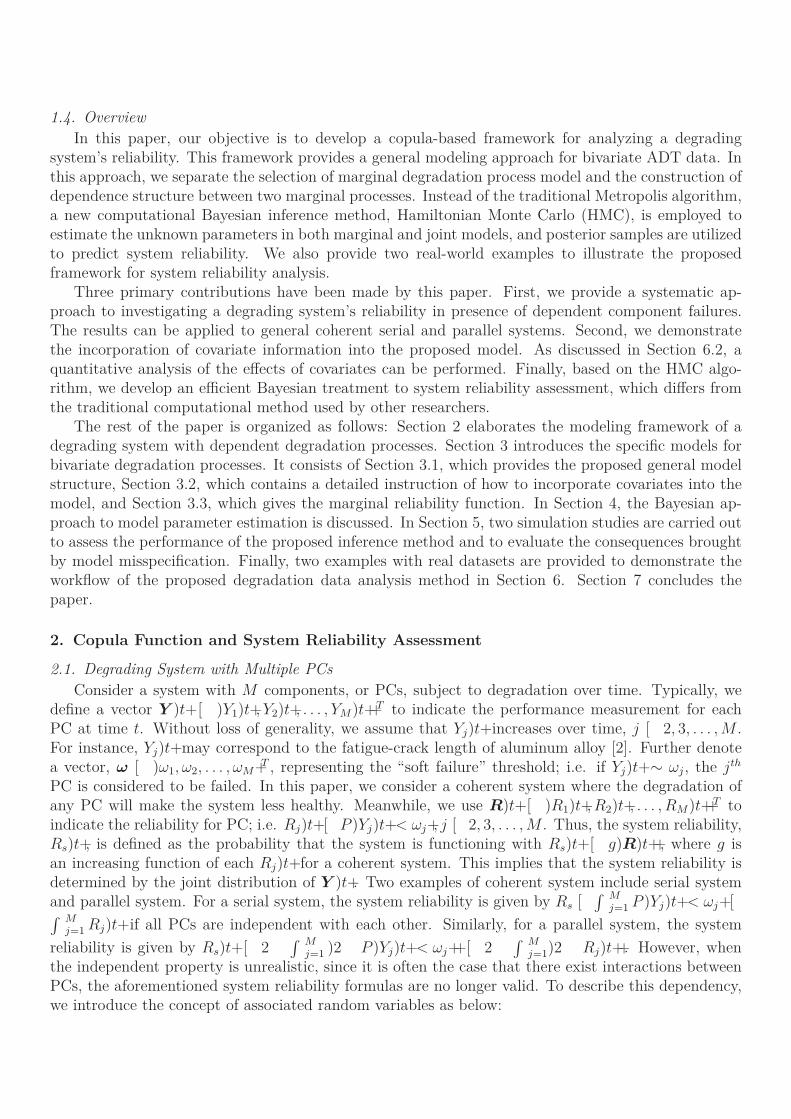
2.2. Copula FunctionA copula is the function that connects the joint distribution function with individual marginal

distribution functions. It is defined as C)u1, u2, . . . , ud+; ]1, 2ˆd ∝ ]1, 2 , which is the joint cumulative

density function (cdf) of a d-dimensional random vector on the unit cube ]1, 2ˆd with uniform marginaldistributions. Mathematically, C)u1, u2, . . . , ud+[ P )U1 ≥ u1, U2 ≥ u2, . . . , Ud ≥ ud+, where Uj →Unif)1, 2+, {j [ 2, 3, . . . , d. These uniform marginal distributions may be transformed from othercontinuous distributions. The following theorem shows the connection between copula and a generalmultivariate distribution.

Sklar’s Theorem [34]: Let X [ )X1, X2, . . . , Xd+T be a random vector with marginal cdfs

F1)x1+, F2)x2+, . . . , Fd)xd+, and let H)x1, x2, ..., xd+be their joint cdf. Define uj [ P )Xj < xj+,{j [ 2, 3, . . . , d. Then, there exists a copula function C such that

C)u1, u2, . . . , ud+[ C)F1)x1+, F2)x2+, . . . , Fd)xd++

[ P )X1 ≥ x1, X2 ≥ x2, . . . , Xd ≥ xd+

[ H)x1, x2, . . . , xd+

(3)

With the cdf of a joint distribution, it is easy to derive its probability density function (pdf) as

h)x1, x2, . . . , xd+[ c)F1)x1+, F2)x2+, . . . , Fd)xd++d

j=1

fj)xj+, (4)

where fj)xj+is the marginal pdf of Xj and c)F1)x1+, F2)x2+, . . . , Fd)xd++is the copula density function,which can be obtained by taking partial derivative of copula function.

The survival function, #C)×+, as defined in [35] is given by

#C)u1, u2, . . . , ud+[ 2 0d∏

k=1

) 2+k∏

1′ i1<i2<×××<ik′ d

Ci1i2×××ik)ui1 , ui2 , . . . , uik+, (5)

with Ci1i2×××ik)ui1 , ui2 , . . . , uik+denoting the marginal of C related to )i1, i2, . . . , ik+.For example, considering a bivariate case, Equation (5) becomes

#C)u1, u2+[ 2 u1 u2 0 C)u1, u2+.

Among all available copulas, there is a popular family of copulas called the Archimedean family.This family admits explicit formulas and they allow modeling variable dependence through an associa-tion parameter. In this paper, we consider the following four widely-used copulas in the Archimedeanfamily: Gumbel copula, Frank copula, Clayton copula, and Joe copula. These copulas hold varioustypes of tail dependence – Gumbel copula and Joe copula have upper tail dependence (λU), Claytoncopula has lower tail dependence (λL), and Frank copula is symmetric with no tail dependence. Insideeach of these copula functions, there is an association parameter, δ, which measures the dependencybetween two variables. The specific functions of these copulas are given as below:

• Gumbel copula: C)u1, u2+[ g x} ]) mpi u1+δ 0 ) mpi u2+

δˆ1δ | , where δ ∀ ]2,∈ +and τ [ 2 2/δ

with λU [ 3 31/δ and λL [ 1;

• Clayton copula: C)u1, u2+[ n e))u δ

1 0 u δ2 2+

1δ , 1

(, where δ ∀ ] 2,∈ +/}1| and τ [ δ

2+δ

with λU [ 1 and λL [ 3 1/δ;

• Frank copula: C)u1, u2+[1δmpi

}2 0 [exp( δu1) 1][exp( δu2) 1]

exp( δ) 1

√, where δ ∀ ) ∈ , 1+

∑)1,∈ +and

τ [ 2 0 5D1(δ) 1δ

with D1)δ+[1δ

⋃δ

0t

et 1dt and λU [ λL [ 1;

• Joe copula: C)u1, u2+[ 2 ])2 u1+δ 0 )2 u2+

δ )2 u1+δ)2 u2+

δˆ1δ , where δ ∀ ]2,∈ +with

λU [ 3 31/δ and λL [ 1.

Note that the relationship between Kendall’s correlation τ and the association parameter δ is also givenfor each of the copulas above. For Joe copula, τ can be approximated by Monte Carlo simulation [36].

2.3. System Reliability from Copula ViewpointRecall that when PCs are not mutually independent, the system reliability, Rs)t+, is determined by

the joint distribution of Y )t+. By introducing the concept of copula, we can develop a straightforward,yet flexible, approach for constructing the joint distribution of Y )t+. More importantly, since thecopula function generates this joint distribution via the cdfs of marginal random variables, it providesan intuitive method of combining marginal reliabilities and dependence structure to calculate thesystem reliability. Figure 2 illustrates the construction of bivariate joint distribution via a copulafunction, as well as the system reliability derived directly from a copula.

Figure 2: Construction of Bivariate Joint Distribution via Copula Function.

Therefore, from the copula perspective, the reliability of a degrading system with dependent PCscan be described by the following theorem:

Theorem 2. Consider a degrading coherent system with M positively associated performancemeasurements of components at time t, i.e. Y )t+[ )Y1)t+, Y2)t+, . . . , YM)t++

T , d ∼ 3. Let R)t+[)R1)t+, R2)t+, . . . , RM)t++

T denote the marginal reliabilities at time t. Then, the system reliabilitysatisfies the following properties:

1. For a serial system,

Rs)t+[ P )Y1)t+< ω1, Y2)t+< ω2, . . . , YM)t+< ωM+

[ C R1)t+, R2)t+, . . . , RM)t+=θCop

(.

(6)

2. For a parallel system,

Rs)t+[ 2 P )Y1)t+> ω1, Y2)t+> ω2, . . . , YM)t+> ωM+

[ 2 #C R1)t+, R2)t+, . . . , RM)t+=θCop

(.

(7)

where θCop is a set of parameters in the copula function.Note that if all PCs are mutually independent, the system reliability is

∫ Mj=1 Rj)t+and 2

∫ Mj=1)2

Rj)t++for a series system and a parallel system, respectively, and they can be derived from a indepen-dence copula, defined as C)u1, u2, . . . , uM+[

∫ Mj=1 uj.

It is also noticed that by introducing copula functions, three attractive features to data analysisare immediately obtained: 1) The marginal distributions of individual variables and their dependencystructure can be separated. This feature will reduce the difficulty of parameter estimation. 2) Thereis no restriction on marginal model. It can be any distribution model that provides the best fit tothe data. Thus, we will not be restricted to the same marginal distribution for different PCs. 3)The system reliability can be evaluated analytically once the marginal cdfs or marginal reliabilitiesare given. Therefore, utilizing a copula to characterize a degrading system will greatly facilitate thesystem reliability analysis.

3. Bivariate Degradation Process

3.1. A General Multivariate ModelConsider an ADT of N test units with M PCs. There are L environmental stress variables and K

distinct time points when each test unit’s degradation was measured. The degradation measurementis denoted by yij)tk+or yijk for the ith test unit, jth PC, and kth time point, and the stress vector foreach test unit is denoted by si. As a result, the degradation dataset for the jth PC is given by

Y j [ )yj, t,S+[

⎞⎟⎟⎟⎟⎟⎟⎟⎟⎟⎟⎟⎟⎟⎟⎠

y1j1 t1 s∞1y1j2 t2 s∞1

... ... ...y1jK1 tK1 s∞1y2j1 t1 s∞2

... ... ...yijKi

tKis∞i

... ... ...yNjKN

tKNs∞N

⎧∏∏∏∏∏∏∏∏∏∏∏∏∏∏⎜, {j [ }2, 3, . . . ,M | ,

where si [ )s1, s2, . . . , sL+∞represents the values of stress variables for the ith test unit and Ki is

the total number of measurements for the ith unit. Ki may vary from unit to unit. Under thestochastic process modeling framework, we work on degradation increments, which are defined asΛyij)tk+[ yij)tk+ yij)tk 1+. According to [37], the stochastic process modeling is favored than thegeneral path modeling of degradation data because it is capable of including unexplainable randomnessresided in the data, which may be caused by some unobserved environmental factors or some unknowneffects of observed environmental factors. Based on the independent increment and infinite divisibilityproperties of Lévy process [38], a degradation dataset can be analyzed by using the following generalmultivariate model structure:

(ΔYi1(tk),ΔYi2(tk), . . . ,ΔYiM (tk))→C F1(Δyi1(tk)), F2(Δyi2(tk)), . . . , FM (ΔyiM (tk));θCop

(,

ΔYij(tk)→MDP(Y j ;θMarj ),

(8)

where C(×) is a copula function, representing the joint cdf of PCs, and Fj(Δyij(tk)), θCop, and θMarj are the

marginal cdf of individual PC, the parameters of copula function and the parameters of marginal degradationprocess (MDP), respectively. The MDPs in consideration here are Wiener process, Gamma process and InverseGaussian (IG) process, and they are given as follows:

MDP)Y j=θMarj +;

⎩⎝⎪⎝⎨ΛYij)tk+→N αjh)si+ΛΦj)tk=γj+, β

2jh)si+ΛΦj)tk=γj+

(ΛYij)tk+→Ga )αjh)si+ΛΦj)tk=γj+, βj+

ΛYij)tk+→IG )αjh)si+ΛΦj)tk=γj+, βjh)si+2ΛΦj)tk=γj+

2+.

(9)

In Model (8), some popular copula functions, such as those from the Archimedean group, can beconsidered for modeling the dependence structure among PCs, while each MDP can be any one of theunivariate processes listed in (9). To ease the mathematical notation, we use α and β to indicate thetwo parameters in a MDP and use h)×+to represent a function of covariates in the marginal model.Finally, ΛΦ)tk=γj+[ Φ)tk=γj+ Φ)tk 1=γj+, which is the time interval after a power transformation oforiginal time with parameter γj.

Using this general modeling approach, a great amount of bivariate degradation models can beintroduced. For instance, a bivariate degradation model with two different marginal processes, such asa Wiener process and an IG process, are demonstrated below:

)ΛYi1)tk+,ΛYi2)tk++→C )F1)Λyi1)tk++, F2)Λyi2)tk++=δ+,

ΛYi1)tk+→N α1 g x) η/si+Φ1)t=γ1+, β21 g x) η/si+Φ1)t=γ1+

(,

ΛYi2)tk+→IG α2 g x) η/si+Φ2)t=γ2+, β2]g x) η/si+Φ2)t=γ1+2(.

(10)

Here, δ denotes the association parameter between two PCs. Specifically, for PC1, α1 and β1 representthe drift parameter and the diffusion parameter of a Wiener process, respectively. For PC2, α2 and β2

represent the mean and shape parameters of an IG process, respectively. In Model (10), we introducea stress variable, si, to represent the stress level on the ith test unit. If it is thermal stress, a simplifiedArrhenius function can be used to capture the degradation acceleration effect of temperature. Thedetailed explanation of how to include a covariate in degradation analysis will be presented in the nextsection.

3.2. Covariate InformationWhen a product is highly reliable, its degradation rate could be too small to be noticeable under the

normal use condition; thus, ADTs are adopted to expedite the degradation process by subjecting theproduct to some harsher environmental conditions, such as higher temperature or stronger vibration.Other common stress factors could be humidity, electric current, and voltage, etc. These stress factorsare treated as covariates or markers in a statistical model [37]. To evaluate the effect of a covariate,Nelson [39] and Meeker and Escobar [2] discussed several acceleration functions that connect differenttypes of stresses with a product’s lifetime via the knowledge of chemical kinetics.

Five commonly used acceleration functions are listed in Table 1, where parameters ξ and η areproduct or material characteristics. These functions are indeed the link functions that incorporatethe effects of corresponding covariates into a general degradation model. Note that an un-accelerateddegradation test can be viewed as having h)s+[ 2. In engineering applications, choosing a goodlink function requires some domain knowledge of the underlying physical/chemical material changemechanism. In the literature, Doksum and Normand [40] used a linear link function to analyze biomakerdata. Tang et al. [41] also assumed the linear link function and they applied it to analyze a LEDdataset. Padgett and Tomlinson [42] declared that, when linking temperature to a Wiener processmodel, the power law function outperforms the Arrhenius function for analyzing a dataset of carbon-film resistor. When having more than one acceleration factor, Liao and Tseng [43] combined theArrhenius function and the power law function to incorporate both temperature and electric currentin their LED experiments, while Fang et al. [6] considered the Eyring function to integrate two stressvariables, temperature and humidity.

In addition, finding an appropriate way to incorporate the link function into the degradation modelstructure requires the researcher to have a good understanding of the impact of stress factor on modelparameter [37]. For example, to account for the degradation acceleration induced by temperature,Model (10) chooses a multiplicative effect derived from the Arrhenius law on the parameter; i.e.,

Table 1: Common Link Functions forStress Acceleration Relations.

Acceleration Relation Link FunctionLinear relation h)s+[ ξ0 0 ξ1sArrhenius relation h)s+[ ξe η/s

Power Law relation h)s+[ ξsη

Inverse-log relation h)s+[ ξ)mpi s+η

Exponential relation h)s+[ ξeηs

αj g x) η/si+. Furthermore, g x) η/si+and ]g x) η/si+2 are incorporated into the diffusion param-

eter of Wiener process and the shape parameter of IG process, respectively. This indicates that a testunit under higher temperature will have a higher volatility in degradation. Nevertheless, there are anumber of different ways to link parameters to stress variables. For instance, Park and Padgett [10]applied and compared four different link functions on analyzing a carbon-film resistor dataset and afatigue crack size dataset. Peng [15] utilized the Arrhenius relation to involve explanatory variablesinto the Inverse Normal-Gamma mixture (ING) model and argued that it was a proportional meanmodel. Tang et al. [44] and Sun et al. [45] made use of the Arrhenius relation in modeling the driftparameter of a nonlinear Wiener process.

3.3. Marginal ReliabilityFor an individual PC, its marginal reliability function is relatively easy to obtain from a univariate

stochastic process model. Without loss of generality, we let a degradation process start from Y )1+[1 and the failure time is the time when Y )t+first pass a threshold, ω. For example, Folks andChhikara [46] proved that the first passage time (Tω) of a Wiener process followed an inverse Gaussiandistribution, IG)ω/α, ω2/β2+. The marginal reliability functions of the three stochastic processes listedin (9) are summarized as below:

• Wiener process

R)t+[ P )Tω > t+[ P )Y )t+< ω+

[ 2 ¯

]2

β

Φ)t=γ+

h)s+)αh)s+Φ)t=γ+ 2+

{

g x

)3αω

β2

[¯

]2

β

Φ)t=γ+

h)s+)αh)s+Φ)t=γ+0 2+

{=

(11)

• Gamma process

R)t+[ P )Tω > t+[ P )Y )t+< ω+

[2

αh)s+Φ)t=γ+(γ αh)s+Φ)t=γ+, βω

(=

(12)

• IG process

R)t+[ P )Tω > t+[ P )Y )t+< ω+

[ ¯

]√βh)s+2Φ)t=γ+2

ω

)ω

αh)s+Φ)t=γ+2

[{

0 g x

)3βh)s+Φ)t=γ+

α

[¯

] √βh)s+2Φ)t=γ+2

ω

)ω

αh)s+Φ)t=γ+0 2

[{.

(13)

Here, Φ)t=γ+[ tγ, a power transformation on the time scale.

4. Bayesian Approach to System Reliability Analysis

In Sections 2 and 3, we provide an overview of system reliability analysis with generally dependentdegradation PCs. To systematically analyze a product with multiple, generally correlated, degradingPCs, we propose a two-step Bayesian approach, which is illustrated by a flowchart in Figure 3. Inthe first step our goal is to select the best multivariate degradation model to fit the data and to infermodel parameters. Then, in the second step we utilize the posterior samples of model parameters toconduct system reliability analysis.

Step 1: Degradation Modeling and Parameter EstimationWhen a bivariate degradation process is modeled by the modeling framework as in (8), we may

group these model parameters as θMar1 [ }α1, β1, γ1,η

∞1| , θMar

2 [ }α2, β2, γ2,η∞2| , and θCop [ δ. Thus,

the log-likelihood function is given by

mo L)θMar1 ,θMar

2 ,θCop+[N∏i=1

Ki∏k=1

mo c F1)Λyi1)tk+=θMar1 +, F2)Λyi2)tk+=θ

Mar2 +=θCop

(0

N∏i=1

2∏j=1

Ki∏k=1

mo fj)Λyij)tk+=θMarj +.

(14)

It is difficult to directly maximize Equation (14) so as to find the maximum likelihood estimation(MLE) of model paramters. However, the separation of marginals and copula density suggests that wecan firstly estimate the marginal parameters and then infer the copula association parameter, leadingto a two-stage approach. The basic idea of this approach originates from the work provided by Joe[47]. However, if the problem has a complex data structure and large data size (e.g., the motivatingexample aforementioned contains more than 4, 111 data points), it is difficult find a numerically stablesolution by MLE. Instead, by leveraging the flexibility of computational Bayesian methods, we developa Bayesian version of the two-stage inference technique. This two-stage Bayesian inference method isillustrated in the upper part of Figure 3.

First, we select the best marginal model for each PC. The univariate models listed in (9) are consid-ered as potential candidates. Following the Bayesian inference method, the mathematical expressionof posterior distribution of MDP parameters is given by

p)θMarj Yj+∞π)θMar

j +≡ f)Yj θMarj +

∞π)θMarj +≡

N

i=1

Kik=1

f)Λyij)tk+θMarj +, j [ 2, 3.

(15)

Figure 3: Flowchart of Two-step Bayesian Approach for System Reliability Analysis.

After the parameters embedded in each model are estimated, the Bayesian Information Criterion (BIC),which is given below, can be employed to compare their goodness-of-fit:

BIC [ 3mo)aL+0 pmo)n+,

where p and n are the number of parameters and the sample size, respectively.Next, we select the best joint model via copula functions. Based on the marginal mod-

els determined in the first stage, the corresponding pairs of cdfs for degradation increments,F1)Λyi1k={θ1

Mar+, F2)Λyi2k={θ2

Mar+(

are computed and they are treated as sample data for inferringcopula functions. By the Bayesian approach, the posterior distribution of copula parameter is givenby

p)θCop Y1,Y2+∞π)θCop+≡N

i=1

Kik=1

c)F1)Λyi1)tk+={θ2

Mar+, F2)Λyi2)tk+={θ2

Mar+=θCop

(. (16)

To construct these posterior distributions as formulated in Equations (15) and (16), we need toemploy the Markov chain Monte Carlo (MCMC) technique to generate the posterior samples of pa-rameters of interest and to obtain the point or interval estimations by summarizing these posterior

samples. Several previous publications, including [28], [29], and [48], utilized the well-known Metropolisalgorithm, which is described below.

Algorithm 1: Metropolis Algorithm [49]Given a current sample θ(s), a new sample θ(s+1) is obtained as follows:

1. Sample θ≤→J)θ θ(s)+, where J is a proposal distribution;2. Compute the acceptance ratio

r [p)θ≤Data+

p)θ(s) Data+[

π)θ≤+L)θ≤Data+

π)θ(s)+L)θ(s) Data+=

where Data represents a set of observed data points.3. Let

θ(s+1) [

⎛θ≤with probability n lo)r, 2+

θ(s) with probability 2 n lo)r, 2+.

This step can be accomplished by sampling u→Uniform)1, 2+and setting θ(s+1) [ θ≤, if u < r,and setting θ(s+1) [ θ(s), otherwise.

In those papers, the BUGS family of Bayesian inference platforms [50] were used. The BUGS soft-ware typically sets the proposal distribution, J , as either a multivariate normal distribution or severalunivariate normal distributions centering at the current sample. Essentially, the Metropolis algorithmpresents a random-walk behavior, which results in inefficiency when exploring a high-dimensional pos-terior surface. For example, the running time of Algorithm 1 until convergence for the aforementionedmotivating example will be extremely long. To expedite the inference process, we choose anotherfamily of MCMC algorithms called the Hamiltonian Monte Carlo (HMC). Being closely related tothe Hamiltonian mechanics, HMC treats the parameter of interest, θd∗ 1, as a position variable andintroduces an auxiliary variable, pd∗ 1, as a momentum variable. Meanwhile, the potential energy isdefined as the negative posterior log-likelihood, i.e. U)θ+[ mo L)θ Data+, and the kinetic energy isdefined as K)p+[ pTp

2. According to the property of energy conservation of Hamiltonian dynamics,

the Hamiltonian function, H)θ,p+[ U)θ+0 K)p+, should remain invariant along the whole periodof movement. In other words, under the framework of a Hamiltonian system, the energy is mutuallytransferred between the potential energy and the kinetic energy with the change of system state. Interms of determining P )θ,p+, which is the probability indicating the system being at a certain state)θ,p+, the concept of a canonical distribution from statistical mechanics can be applied. This is givenby

P )θ,p+[2

Zg x

)H)θ,p+

T

[[

2

Zg x

)U)θ+

T

[g x

)K)p+

T

[[

2

Zπ)θ+L)θ Data+g x

)K)p+

T

[∞π)θ+L)θ Data+g x

)pTp

3

[Gaussian kernel

≤ π)θ+L)θ Data+N)p 0, I+,

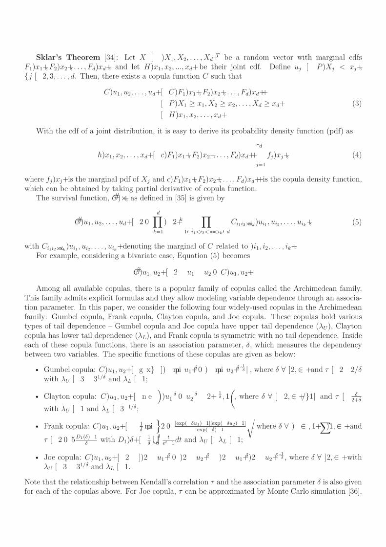
where Z is a normalizing constant, and T is the temperature of the system and it can be assumed tobe 2. In summary, the HMC algorithm is given by Algorithm 2 below.

Algorithm 2: HMC Algorithm [51]Given a current sample θ(s), a new sample θ(s+1) is obtained as follows:

1. Sample p(s) →N)0, I+;2. Run Leapfrog algorithm at )θ(s),p(s)+for L steps with step size ε to obtain proposed state )θ≤,p≤+:

2.1 Make a half step for momentum at the beginning:

p≤i [ p≤i )ε/3+∂U

∂θi)θ(s)+, {i [ 2, . . . , d.

2.2 Alternate L times with full step for position:

θ≤i [ θ(s)i 0 εp≤i , {i [ 2, . . . , d.

2.3 Make a half step for momentum at the end:

p≤i [ p≤i )ε/3+∂U

∂θi)θ≤+, {i [ 2, . . . , d.

Then, θ≤ [ )θ≤1, θ≤2, . . . , θ

≤d+and p≤ [ )p≤1, p

≤2, . . . , p

≤d+.

Thus, H)θ(s),p(s)+[ U)θ(s)+0 K)p(s)+and H)θ≤,p≤+[ U)θ≤+0 K)p≤+.3. Compute the acceptance ratio

r [P )θ≤,p≤+

P )θ(s),p(s)+[ g x

)H)θ(s),p(s)+ H)θ≤,p≤+

([

π)θ≤+L)θ≤Data+N)p≤0, I+

π)θ(s)+L)θ(s) Data+N)p(s) 0, I+=

where Data represents a set of observed data points.4. Let

θ(s+1) [

⎛θ≤with probability n lo)r, 2+

θ(s) with probability 2 n lo)r, 2+.

This step can be accomplished by sampling u→Uniform)1, 2+and setting θ(s+1) [ θ≤ if u < rand setting θ(s+1) [ θ(s) otherwise.

In Algorithm 2, the Leapfrog algorithm at Step 2 is a method of numerical approximation tocalculate θ and p according to the Hamiltonian equations. HMC differs from the Metropolis algorithmon two aspects: 1) HMC adds two normal densities into the acceptance ratio calculation. This maylook like a trivial difference, but the resulted ratio value of HMC is much higher due to the subtledifference between H)θ(s),p(s)+and H)θ≤,p≤+, which is purely caused by the approximation error ofLeapfrog algorithm. In fact, there should be no change due to the property of energy conservationof Hamiltonian system. Thus, with a higher sample acceptance rate, HMC is more efficient thanthe Metropolis algorithm. 2) Apparently, in Step 2 of the HMC algorithm, the gradient of posteriordistribution is utilized to generate new momentum variable, p. The Metropolis algorithm simply uses aproposal distribution that is not directly related to the target distribution. Thus, given an equal lengthof running steps, HMC should reach to the steady state much sooner than the Metropolis algorithm.

HMC is able to find a lower value of negative log-likelihood in fewer number of iterations and has theautocorrelation of samples decayed much faster [52]. In this paper, we use a HMC software packagecalled RStan [53]. In addition, we use non-informative prior distributions, such as uniform distributionswithin relatively large intervals.

Step 2: System Reliability AnalysisAfter the joint degradation model was established, the system reliability is to be calculated. The

lower part of Figure 3 shows the procedure of reliability prediction. Given the posterior samples ofmodel parameters after a burn-in period, a total number of S samples are drawn. Then, the marginaland system reliability are calculated based on Equations (11) to (13) and Equations (6) and (7),respectively. Again, using these samples, both the point and interval estimation of reliability can beobtained.

5. Simulation Study

5.1. Performance of the Proposed Inference MethodIn this section, we conduct a Monte Carlo simulation study to demonstrate the performance of the

proposed two-stage system reliability analysis approach. For illustration, we simulate three differentbivariate models with heterogeneous marginals and they are the Frank copula with Wiener-Gammacombination (Simulation Model %2 or SM%2), the Gumbel copula with Gamma-IG combination(SM%3), and the Clayton copula with Wiener-IG combination (SM%4).

SM%2 ; )ΛYi1)tk+,ΛYi2)tk++→CFrank )F1)Λyi1)tk++, F2)Λyi2)tk++=21+,

ΛYi1)tk+→N)2.6Λ tk, 1.62Λ tk+,

ΛYi2)tk+→Ga)4Λ tk, 3+,

SM%3 ; )ΛYi1)tk+,ΛYi2)tk++→CGumbel )F1)Λyi1)tk++, F2)Λyi2)tk++=4+,

ΛYi1)tk+→Ga)5Λ tk, 4+,

ΛYi2)tk+→IG)3Λ tk, 6Λ t2k+,

SM%4 ; )ΛYi1)tk+,ΛYi2)tk++→CClayton )F1)Λyi1)tk++, F2)Λyi2)tk++=3+,

ΛYi1)tk+→N)3Λ tk, 1.42Λ tk+,

ΛYi2)tk+→IG)2.6Λ tk, 5Λ t2k+,

where Λ tk [ tk tk 1.

Algorithm 3: Random Degradation Value Generation1. for i [ 2 to N do2. for k [ 2 to K do3. Generate )u1, u2+from C)u1, u2 δ+4. Calculate Λyijk through F 1

j )uj θMarj ) for j [ 2, 3

5. Set yijk [ yij,k 1 0 Λyijk, where yij0 [ 1 for j [ 2, 36. end for7. end for

To ease the computational burden, we set N [ 2, h)s+[ 2, Φ)t+[ t and the number of degradationmeasurements to be K [ 41, 66, or 91. We repeat each simulated process 2, 111 times. To initialize

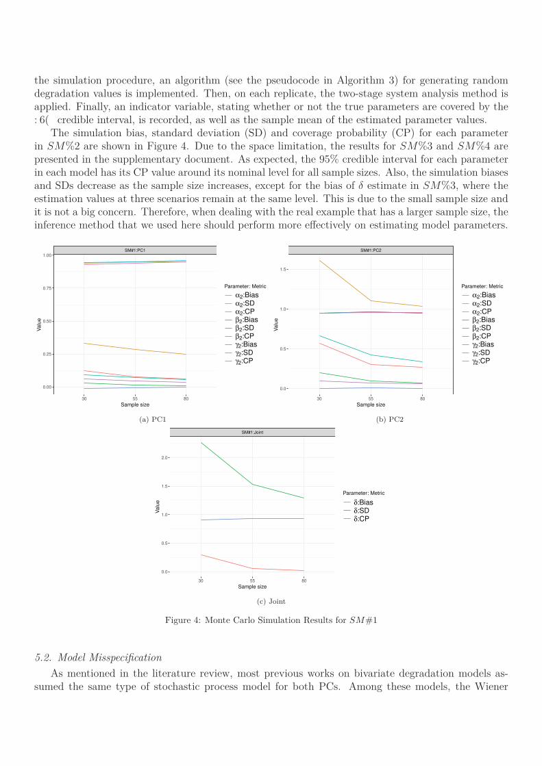
the simulation procedure, an algorithm (see the pseudocode in Algorithm 3) for generating randomdegradation values is implemented. Then, on each replicate, the two-stage system analysis method isapplied. Finally, an indicator variable, stating whether or not the true parameters are covered by the: 6( credible interval, is recorded, as well as the sample mean of the estimated parameter values.

The simulation bias, standard deviation (SD) and coverage probability (CP) for each parameterin SM%2 are shown in Figure 4. Due to the space limitation, the results for SM%3 and SM%4 arepresented in the supplementary document. As expected, the 95% credible interval for each parameterin each model has its CP value around its nominal level for all sample sizes. Also, the simulation biasesand SDs decrease as the sample size increases, except for the bias of δ estimate in SM%3, where theestimation values at three scenarios remain at the same level. This is due to the small sample size andit is not a big concern. Therefore, when dealing with the real example that has a larger sample size, theinference method that we used here should perform more effectively on estimating model parameters.

SM#1:PC1

30 55 80

0.00

0.25

0.50

0.75

1.00

Sample size

Val

ue

Parameter: Metric

α2:Biasα2:SDα2:CPβ2:Biasβ2:SDβ2:CPγ2:Biasγ2:SDγ2:CP

(a) PC1

SM#1:PC2

30 55 80

0.0

0.5

1.0

1.5

Sample size

Val

ue

Parameter: Metric

α2:Biasα2:SDα2:CPβ2:Biasβ2:SDβ2:CPγ2:Biasγ2:SDγ2:CP

(b) PC2

SM#1:Joint

30 55 80

0.0

0.5

1.0

1.5

2.0

Sample size

Val

ue

Parameter: Metric

δ:Biasδ:SDδ:CP

(c) Joint

Figure 4: Monte Carlo Simulation Results for SM#1

5.2. Model MisspecificationAs mentioned in the literature review, most previous works on bivariate degradation models as-

sumed the same type of stochastic process model for both PCs. Among these models, the Wiener

processes with various copula functions are often employed due to its close relationship with normaldistribution. However, if the combination of a non-monotonic process and a monotonic process, suchas the Wiener-Gamma combination, is present, accepting the Wiener-Wiener model a priori with-out an examination of data may result in a bad joint distribution model. In this simulation study,we simulate three degradation processes that are generated by the Wiener-Gamma combination withvarious copulas and parameters. To reduce the variability caused by simulation, we set N [ 41 andK [ 41, leading to a relatively large sample size. Similarly to the previous study, we let h)s+[ 2. Thedegradation data are generated from models SM%5, SM%6, and SM%7 using the parameter valuesas shown below. Specifically, we set the power transformation to be as Φ)tk=γ+[ tγk tγk 1, where γcontrols the time scale. Different γ values (being less than or greater than 2) will adjust the shapeof degradation path (i.e., convex, linear, or concave). In addition, Gumbel copula, Frank copula andClayton copula are applied to realize various types of degradation process dependency. The results ofparameter estimation are included in the supplementary document.

SM%5 ; )ΛYi1)tk+,ΛYi2)tk++→CGumbel )F1)Λyi1)tk++, F2)Λyi2)tk++=4+,

ΛYi1)tk+→N)2.6Φ)tk=1.7+, 1.62Φ)tk=1.7++,

ΛYi2)tk+→Ga)4Φ)tk=1.6+, 3+,

SM%6 ; )ΛYi1)tk+,ΛYi2)tk++→CFrank )F1)Λyi1)tk++, F2)Λyi2)tk++=3+,

ΛYi1)tk+→N)2.6Φ)tk=2+, 1.62Φ)tk=2++,

ΛYi2)tk+→Ga)4Φ)tk=2+, 3+,

SM%7 ; )ΛYi1)tk+,ΛYi2)tk++→CClayton )F1)Λyi1)tk++, F2)Λyi2)tk++=3+,

ΛYi1)tk+→N)2.6Φ)tk=2.3+, 1.62Φ)tk=2.3++,

ΛYi2)tk+→Ga)4Φ)tk=2.5+, 3+,

Figures 5, 6, and 7 show the degradation paths of simulated data, as well as the contour plotsof model densities for the degradation increments from 1 to 2 hour and from 2: to 31 hours. Oneach contour plot, the densities from both the true model and the estimated Wiener-Wiener modelare depicted by using blue solid lines and green dashed lines for them, respectively. Based on thesesimulation results, several interesting findings can be drawn.

First, one can see that the bivariate degradation model that combines copula functions and stochas-tic process models is able to capture the dynamics of degradation process. This can be seen by thecontour plots in two time phases. As shown by the degradation paths, the value of time scale trans-formation parameter, γ, directly determines the shape of degradation path. If γ [ 2, the degradationpath indicates a linear trend over time as shown in Figure 6a. In other words, the degradation rateremains constant over the whole lifetime. However, if γ < 2, it demonstrates a concave trend as shownin Figure 5a, which has a decreasing degradation rate and is going to reach a saturation point eventu-ally. On the contrary, Figure 7a shows a convex trend that exhibits accelerated deterioration. For alinear degradation process, its contour plots remain the same regardless of the phases of degradation.This can be observed from Figures 6b and 6c and this is because the parameters of marginal modelsdo not change with the passage of time. But, for the case of SM%5, the density gradually moves to aborder axis due to the slowdown of degradation process, as shown in Figures 5b and 5c.

One should also notice how the tail dependence is reflected in these figures. For example, sinceadmitting only upper-tail dependence, the contour lines of Gumbel copula indicates a sharper shape

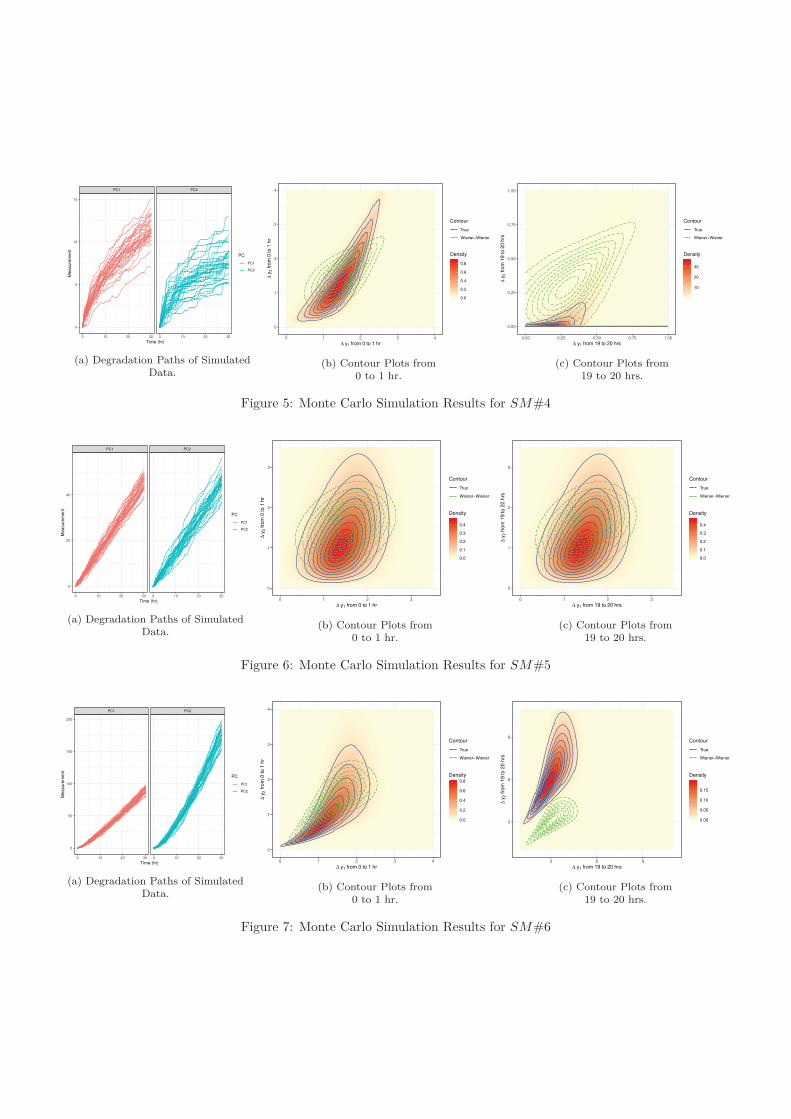
PC1 PC2

0 10 20 30 0 10 20 30

0

5

10

15

Time (hr)

Mea

sure

men

t

PC

PC1

PC2

(a) Degradation Paths of SimulatedData.

0

1

2

3

4

0 1 2 3 4Δ y1 from 0 to 1 hr

Δy 2

from

0to

1hr

Contour

True

Wiener−Wiener

0.0

0.2

0.4

0.6

0.8

Density

(b) Contour Plots from0 to 1 hr.

0.00

0.25

0.50

0.75

1.00

0.00 0.25 0.50 0.75 1.00Δ y1 from 19 to 20 hrs

Δy 2

from

19to

20hr

s

Contour

True

Wiener−Wiener

10

20

30

Density

(c) Contour Plots from19 to 20 hrs.


PC1 PC2

0 10 20 30 0 10 20 30

0

20

40

Time (hr)

Mea

sure

men

t

PC

PC1

PC2


0

1

2

3

0 1 2 3Δ y1 from 0 to 1 hr

Δy 2

from

0to

1hr

Contour

True

Wiener−Wiener

0.0

0.1

0.2

0.3

0.4

Density


0

1

2

3

0 1 2 3Δ y1 from 19 to 20 hrs

Δy 2

from

19to

20hr

s

Contour

True

Wiener−Wiener

0.0

0.1

0.2

0.3

0.4

Density



PC1 PC2

0 10 20 30 0 10 20 30

0

50

100

150

200

Time (hr)

Mea

sure

men

t

PC

PC1

PC2


0

1

2

3

4

0 1 2 3 4Δ y1 from 0 to 1 hr

Δy 2

from

0to

1hr

Contour

True

Wiener−Wiener

0.0

0.2

0.4

0.6

0.8Density


3

6

9

3 6 9Δ y1 from 19 to 20 hrs

Δy 2

from

19to

20hr

s

Contour

True

Wiener−Wiener

0.00

0.05

0.10

0.15

Density



F1(∆ y1)

F2(∆

y2)

0.0

0.2

0.4

0.6

0.8

1.0

0.0 0.2 0.4 0.6 0.8 1.0

0.0

0.2

0.4

0.6

0.8

1.0

(a) Contour Plot.

0.0 0.2 0.4 0.6 0.8 1.0

0.0

0.2

0.4

0.6

0.8

1.0

F1(∆ y1)

F2(∆

y2)

(b) Scatter Plot.

Figure 8: Simulated cdfs of Degradation Increments for SM#4.

F1(∆ y1)

F2(∆

y2)

0.0

0.2

0.4

0.6

0.8

1.0

0.0 0.2 0.4 0.6 0.8 1.0

0.0

0.2

0.4

0.6

0.8

1.0

(a) Contour Plot.

0.0 0.2 0.4 0.6 0.8 1.0

0.0

0.2

0.4

0.6

0.8

1.0

F1(∆ y1)

F2(∆

y2)

(b) Scatter Plot.


F1(∆ y1)

F2(∆

y2)

0.0

0.2

0.4

0.6

0.8

1.0

0.0 0.2 0.4 0.6 0.8 1.0

0.0

0.2

0.4

0.6

0.8

1.0

(a) Contour Plot.

0.0 0.2 0.4 0.6 0.8 1.0

0.0

0.2

0.4

0.6

0.8

1.0

F1(∆ y1)

F2(∆

y2)

(b) Scatter Plot.


in the upper right corner in Figure 5b. The same pattern is present in the lower left corner in Figure7b for Clayton copula. To fully present such features, in Figures 8-10, we provide both the contourplots and scatter plots of cdfs of the degradation increments simulated from the three different copulamodels. As shown in Figure 8b, the simulated data points by SM%5 clustered around the right uppercorner more compactly, where the pattern exists in the left lower corner as shown in Figure 10b. Onthe contrary, due to the symmetric feature of Frank copula, the simulated data points spread over thewhole space, as shown in Figure 9b.

Lastly, and most importantly, it is noticed that if both marginals are decided to be Wiener processesa priori, the resulted joint density will be inconsistent with the true density. The difference will becomelarger and larger along the time if the degradation rate is not constant, because the time scale functionwill exaggerate the deficiency of a wrongly chosen model over time. For instance, in Figure 7b, thecontour lines of the true model and the estimated model still overlap at the starting time, but theywill be almost totally separated at the interval of 2: to 31 hours, as shown in Figure 7c. The Wiener-Wiener model would underestimate the degradation increment for y2 by about 61( . Therefore, onecan see that if the bivariate model is misspecified as a Wiener-Wiener combination, serious bias onthe inference of the joint distribution would result. In such case, a misleading prediction of systemreliability will be produced as well.

6. Applications

As we have shown, the proposed framework integrates the copula theory with general system relia-bility assessment, which allows for a straightforward interpretation of the multivariate model derived.Through the HMC-based Bayesian approach we proposed, the system reliability can be efficiently quan-tified. To apply the modeling framework to real examples, we design the following analysis procedure.

Step 1: Dependence AnalysisGiven a degradation dataset, a nonparametric dependence analysis is first performed to check the

rank correlation between two PCs. This step should be accompanied by the scatter plot function inmost statistical software. If its rank correlation is high, a bivariate degradation model is needed forfurther quantitative analysis. Relevant implementations in R can be found in [54].

Step 2: Degradation Modeling and Parameters EstimationHere, we build the bivariate degradation model as described in Section 4. Specifically, the two-stage

Bayesian inference method is implemented to infer model parameters and to select the joint model.

Step 3: System Reliability AnalysisFinally, the system reliability analysis, as described in the lower part of Figure 3, can be carried

out.

6.1. LED DegradationIn this example, we make use of the LED lamp dataset drawn from Chaluvadi’s doctoral thesis

[55]. This dataset presents a degradation testing result of LED lamps, of which lighting intensity ismeasured every 61 hours under a stress level of 51mA current. This dataset has also been analyzedby other researchers. For example, Ye et al. [56] and Tang et al. [44] did univariate modeling basedon Wiener process, and Hao et al. [32] constructed a bivariate model using Frank copula with Gammaprocess as marginals.

To demonstrate the bivariate stochastic process modeling process, similarly to Hao et al. [32], wesplit the LED dataset into two streams as if the first half came from PC1 and the second half from

Table 2: LED Degradation Test Data.

Inspection Time (hrs)Unit 0 50 100 150 200 250PC1

1 100 86.6 78.7 76.0 71.6 68.02 100 82.1 71.4 65.4 61.7 58.03 100 82.7 70.3 64.0 61.3 59.34 100 79.8 68.3 62.3 60.0 59.05 100 75.1 66.7 62.8 59.0 54.06 100 83.7 74.0 67.4 63.0 61.3

PC21 100 73.0 65.0 60.7 58.3 58.02 100 86.2 67.6 62.7 60.0 59.73 100 81.2 65.0 60.6 59.3 57.34 100 66.8 63.3 59.3 57.3 56.55 100 66.1 64.2 59.4 58.0 55.36 100 76.5 61.7 61.3 59.7 56.0

PC2. These data are shown in Table 2. A LED is considered to be failed if the PC1 value is below 20or the PC2 value is below 40, which means ω1 [ 91 and ω2 [ 71. In addition, the degradation pathof each PC for every unit is plotted in Figure 11a. Notice that it is necessary to apply a time scaletransformation due to the nonlinear pattern of degradation path.

Step 1: According to the degradation path plot, one can see that the two PCs share a com-mon change pattern. A dependence check, which computes the concordance between their negativeincrements, would further confirm this observation. As a result, the Kendall’s coefficient of 1.6: in-dicates that there exists a strong dependency between the two PCs. Also, the scatter plot in Figure11b exhibits a strong upper-tail dependency, as the regression slope becomes more prominent in theupper-right corner and it is flat for the data points in the lower-left corner.

60

70

80

90

100

0 50 100 150 200 250

Time (hrs)

Mea

sure

men

t

PC

PC1

PC2

(a) Degradation Path.

r = 0.59 , p = 5.7e−06

0

10

20

30

0 5 10 15 20 25PC1

PC2

(b) Scatter Plot of Marginal Degradation Increments.

Figure 11: Degradation Path and Scatter Plot for LED Degradation Process.

Step 2: The first stage of parameter estimation for each PC is conducted on every MDPs describedin Section 3.1. Their results are shown in Tables 3 and 4. Non-informative priors are utilized. Toaccommodate the nonlinear degradation pattern, we take use of the power transformation of Φ)t=γ+[tγ. The low BIC values of Gamma process indicate that this stochastic process model is suitable forboth PCs .

Table 3: Parameters Estimation for Marginal Models of PC1.

PC1MDP Parameter mean se_mean sd 2.5% 97.5% BIC

Wiener α 3.493 0.022 0.750 2.974 5.268146.641Process β 1.734 0.009 0.342 1.494 2.519

γ 0.446 0.001 0.037 0.371 0.518Gamma α 3.682 0.029 1.255 1.563 6.508

145.055Process β 1.131 0.007 0.299 0.607 1.777γ 0.459 0.001 0.037 0.391 0.539

IG α 3.398 0.022 0.722 2.124 4.913147.010Process β 11.117 0.178 5.589 2.861 25.563

γ 0.452 0.001 0.037 0.386 0.524



Wiener α 9.350 0.098 3.101 4.744 16.969182.730Process β 5.678 0.052 1.638 3.522 9.709

γ 0.284 0.002 0.054 0.177 0.391Gamma α 2.695 0.029 1.111 0.905 5.194

164.682Process β 0.347 0.002 0.096 0.184 0.559γ 0.320 0.001 0.052 0.229 0.434

IG α 8.854 0.079 2.673 4.335 14.742166.091Process β 17.492 0.368 12.902 2.279 48.242

γ 0.301 0.002 0.051 0.215 0.412

Based on the estimation of MDP model parameters, the corresponding cdf of individual PC’sdegradation increments are obtained as )F1)Λyi1)tk++, F2)Λyi2)tk+++. Carrying out the second stage ofstatistical inference, the association parameter of Joe copula can be estimated. As shown in Table 5,this estimated value is 2.9: : . After removing the time scaling effect, this number provides a quantitativemeasurement of the two PCs’ dependency. From this table, one can also see that Frank copula doesnot fit the data as well as Joe copula, because it includes no tail dependence but the data does show aprominent upper tail dependence. Meanwhile, Clayton copula is suitable for the lower tail dependence,thus it leads to the worst fit. Figure 12 demonstrates the contour plots for densities of joint distributionof the degradation increments between the two PCs. From these plots, one can see that the degradationrate is diminishing as time goes on.

Table 5: Parameters Estimation for Joint Models.

JointCopula Parameter mean se_mean sd 2.5% 97.5% τ BIC

Joe δ 1.899 0.010 0.357 1.263 2.652 0.332 -5.632Frank δ 2.201 0.030 1.167 -0.056 4.628. 0.234 0.944

Gumbel δ 1.443 0.006 0.202 1.096 1.889 0.307 -2.346Clayton δ 0.131 0.006 0.211 -0.191 0.601 0.061 4.125

10

20

30

40

50

10 20 30 40 50

Δ y1 from 0 hr to 50 hrs

Δy 2

from

0hr

to50

hrs

0.001

0.002

0.003

0.004

0.005

Density

(a) Interval between 0 and 50 hrs.

0

4

8

12

0 4 8 12

Δ y1 from 200 hrs to 250 hrs

Δy 2

from

200

hrs

to25

0hr

s

0.00

0.02

0.04

0.06

0.08

Density

(b) Interval between 200 and 250 hrs.

Figure 12: Contour Plots of Joint Distribution Density of Degradation Increments.

Step 3: Finally, through implementing the procedure of reliability estimation presented in Figure3, median curves of reliability prediction over the duration of 1 to 4, 111 hours for both the marginaland joint distributions are plotted in Figure 13. As a comparison, the case of independence of two PCsis also presented. It is noted that the independence assumption would underestimate the product’sreliability. For instance, at 2, 111 hours, the predicted reliability using Joe copula is about 1.3, but itwill be 36( less if the two PCs are assumed to be independent. This result is not a surprise becauseTheorem 1 has shown that

∫ Mj=1 Rj)t+≥ Rs)t+. Thus, these findings further verify the necessity of

conducting dependence check in the first step. Furthermore, Figure 14 provides the : 6( credible bandfor the system reliability curve estimated by using Joe copula.

6.2. Polymeric Material DegradationIn this section, we revisit the motivating example to demonstrate the advantage of the proposed

general bivariate degradation model with the incorporation of covariates.Step 1: As stated in Section 1.2, the two PCs, benzene ring mass loss and aromatric C-O are

named as PC1 and PC2. Observing that the degradation paths of both PCs share similar patterns,it is necessary to evaluate their dependency to each other. Since the degradation path is also affectedby some external environmental factors, such as temperature and UV intensity in this example, wehave to evaluate the dependency at the same environmental stress level. We calculate the Kendall’scoefficient of the degradation increments of both PCs for each test unit and compute the average valueat each stress level. It is found that the Kendall’s τ remains around 1.69 across all stress levels, asshown in Figure 15.

0.00

0.25

0.50

0.75

1.00

0 1000 2000 3000Time (hrs)

Rel

iabi

lity

Process

PC1

PC2

Joint_Joe

Independent

Figure 13: Reliability Curves for LEDDegradation Process.

0.00

0.25

0.50

0.75

1.00

0 1000 2000 3000

Time (hrs)

Rel

iabi

lity

Figure 14: 95% Credible Band for Reliability Curveby Joe Copula.

0.0

0.2

0.4

0.6

1 2 3 4 5 6 7 8

Stress Level

Ken

dall’

s co

effic

ient

Stress Level

1 − 25°C 10%

2 − 25°C 40%

3 − 25°C 60%

4 − 25°C 100%

5 − 35°C 10%

6 − 35°C 40%

7 − 35°C 60%

8 − 35°C 100%

Figure 15: Barchart of Average Kendall’s tau at Each Stress Level.

Step 2: Following the dependence analysis, we fit MDPs to each PC’s degradation dataset. TheArrhenius relation is chosen to incorporate the degradation acceleration effect brought by temperatureand a power law relation is used to model the effect by UV intensity [16]. Taking the Wiener processas example, the drift parameter can be written as

α g x

)η1

22716

TEMP 0 384.26

[NDη2ΛΦ)t=γ+.

Tables 6 and 7 show the parameters estimation of marginal models for both PCs. It turns out thatGamma process is the best model for each PC.

The second stage of parameter inference is carried out by considering the four candidate copulaslisted in Section 2.2. The results in Table 8 indicate that Gumbel copula is the best model. Similarlyto the previous example, we provide the contour plot of joint distribution density of degradationincrements in Figure 16. This is done by assuming a stress level of TEMP 30°C and UV Intensity 85%.It can be seen that the two contour plots do not differ much for two different durations because theparameter γ is close to 2.



Wiener α 480.082 13.260 431.709 162.646 1634.755

-11,808.679Process β 0.245×10 2 0.000 0.017×10 2 0.215×10 2 0.280×10 2

η1 -37.545×10 2 0.780×10 3 2.602×10 2 -41.938×10 2 -32.173×10 2

η2 30.227×10 2 0.720×10 3 3.892×10 2 22.968×10 2 38.242×10 2

γ 121.228×10 2 0.590×10 3 2.478×10 2 116.324×10 2 126.027×10 2

Gamma α 1220.323 14.889 778.138 247.657 3269.224

-12,299.737Process β 271.281 14.549×10 2 966.653×10 2 251.713 290.697

η1 -21.360×10 2 0.360×10 3 1.707×10 2 -24.456×10 2 -17.730×10 2

η2 24.734×10 2 0.260×10 3 1.737×10 2 21.411×10 2 28.087×10 2

γ 93.633×10 2 0.190×10 3 1.256×10 2 91.225×10 2 96.082×10 2

IG α 48.880×10 2 1.286×10 2 41.116×10 2 6.799×10 2 155.859×10 2

-11,555.913Process β 60.323 3.811 135.520 0.678 364.094

η1 -13.572×10 2 0.660×10 3 2.051×10 2 -17.343×10 2 -9.337×10 2

η2 19.127×10 2 0.330×10 3 1.654×10 2 16.024×10 2 22.364×10 2

γ 85.653×10 2 0.190×10 3 0.963×10 2 83.769×10 2 87.535×10 2



Wiener α 531.736 15.829 480.608 30.187 1775.501

-10,637.895Process β 0.167×10 2 0.000 0.011×10 2 0.146×10 2 0.191×10 2

η1 -41.780×10 2 0.088×10 2 2.850×10 2 -46.307×10 2 -35.574×10 2

η2 38.013×10 2 0.091×10 2 4.719×10 2 29.106×10 2 47.285×10 2

γ 149.189×10 2 0.056×10 2 2.567×10 2 144.189×10 2 154.199×10 2

Gamma α 903.878 12.225 646.404 165.343 2653.679

-11,467.287Process β 199.416 0.114 7.067 185.498 213.338

η1 -23.848×10 2 0.040×10 2 1.853×10 2 -27.295×10 2 -19.937×10 2

η2 34.345×10 2 0.029×10 2 1.909×10 2 30.550×10 2 38.002×10 2

γ 109.679×10 2 0.024×10 2 1.535×10 2 106.726×10 2 112.708×10 2

IG α 44.905×10 2 1.021×10 2 39.051×10 2 6.625×10 2 154.426×10 2

-10,867.262Process β 38.849 2.034 85.222 0.492 265.431

η1 -16.242×10 2 0.060×10 2 2.103×10 2 -20.293×10 2 -12.078×10 2

η2 34.479×10 2 0.032×10 2 1.674×10 2 31.221×10 2 37.774×10 2

γ 100.229×10 2 0.021×10 2 1.091×10 2 98.166×10 2 102.466×10 2

Table 8: Parameters Estimation of Joint Models.

JointCopula Parameter mean se_mean sd 2.5% 97.5% τ BIC

Joe δ 3.290 0.002 0.078 3.138 3.446 0.551 -2,408.710Frank δ 10.361 0.006 0.249 9.869 10.850 0.675 -2,572.549

Gumbel δ 2.724 0.001 0.050 2.627 2.825 0.633 -3,043.961Clayton δ 1.256 0.001 0.049 1.161 1.353 0.386 -1,560.568

0.00

0.02

0.04

0.06

0.08

0.00 0.02 0.04 0.06 0.08

Δ y1 from 0 day to 10 days

Δy 2

from

0da

yto

10da

ys

0

1000

2000

Density

(a) Interval between 0 and 10 days.

0.00

0.02

0.04

0.06

0.08

0.00 0.02 0.04 0.06 0.08

Δ y1 from 140 days to 150 days

Δy 2

from

140

days

to15

0da

ys

0

500

1000

1500

2000

2500

Density

(b) Interval between 140 and 150 days.

Figure 16: Contour Plots of Joint Distribution Density of Degradation Incrementsat TEMP 30 °C and UV Intensity 85%.

Step 3: Lastly, we provide the point and interval predictions of reliability for the duration of thefirst 611 days. For the polymeric degradation data, we use a threshold ω1 [ 1.5 and ω2 [ 1.6for PC1 and PC2, respectively, and treat it as a serial system. Correspondingly, Figure 17 shows thereliability curves for both marginal processes and joint models. Again, if the two PCs are assumed tobe independent to each other, the resulting reliability prediction will be below the level when they arecorrelated. Specially, we compare the material’s reliability under two different environmental conditions– TEMP 30 °C and UV Intensity 85% v.s. TEMP 20 °C and UV Intensity 50%. One may regardthese two conditions as one in Phoenix, AZ (where the weather is sunny and hot) and the other onein Raleigh, NC (where the weather is mild). The polymeric material’s lifetime in Raleigh is expectedto be longer. The median lifetime in Phoenix (see Figure 18a) is about 281 days, while in Raleighit will be more than 211 days longer (see Figure 18b). It is also obvious that, due to having moredegradation data available in this example, the : 6( credible band is much narrower here than theprevious example.

0.00

0.25

0.50

0.75

1.00

0 100 200 300 400 500Time (days)

Rel

iabi

lity

Process

PC1

PC2

Joint_Gumbel

Independent

(a) TEMP 30 °C and UV Intensity 85%.

0.00

0.25

0.50

0.75

1.00

0 100 200 300 400 500Time (days)

Rel

iabi

lity

Process

PC1

PC2

Joint_Gumbel

Independent

(b) TEMP 20 °C and UV Intensity 50%.

Figure 17: Reliability Curves for Polymeric Degradation Process.

0.00

0.25

0.50

0.75

1.00

0 100 200 300 400 500

Time (days)

Re

liab

ility

(a) TEMP 30 °C and UV Intensity 85%.

0.00

0.25

0.50

0.75

1.00

0 100 200 300 400 500

Time (days)

Re

liab

ility

(b) TEMP 20 °C and UV Intensity 50%.

Figure 18: 95% Credible Band for Reliability Curve.

7. Conclusions

A degrading system may involve multiple components or PCs that apparently have interactions orshare a common failure mechanism. In such case, cares must be taken to consider the PC dependencywhen we analyze system reliability. In previous research, the choice of bivariate joint distributionwas often pre-determined, which was unfortunately inappropriate in most cases, especially when themarginals are subject to different distributions. By introducing copula functions, we are able to providea complete theoretical framework to investigate the effect of PC dependency on system reliability.Within this modeling framework, a flexible class of bivariate stochastic process-based degradationmodels are proposed and they include a variety of marginal degradation processes and incorporatestress covariates. In addition, an efficient Bayesian inference method, HMC, is implemented in thispaper, which is novel for degradation data analysis. The consequences of model misspecification arethoroughly studied in Section 5.2. The different types of tail dependence of copula functions thatmimic bivariate degradation patterns are discussed too. Two real examples are used to demonstratethe superiority of our approach.

Beyond the scope of current study, there are several other issues worth of a further investigation.For instance, it is our interest to investigate the inference method when some random effects accountingfor the unit-to-unit variation are included in the model. Endowing the analysis with a goodness-of-fittest on multivariate degradation models is intended to be conducted too. This task is not easy; buttailored test statistics are possible to be built based on several existing test methods about copulas,such as the Cramér-von Mises statistic [57]. Also, how to model a system with multiple componentsin a complex structure or a multi-component system with multiple PCs requires an extensive research.Moreover, the extension of the current work to a more general setting, such as incorporating bothtime-to-failure data and binary pass-fail data, need be further developed.

Acknowledgement

The research by the first and second authors were partially supported by NSF grant 1726445 andthe research by the third author was partially supported by NSF grant 1838271.

Appendix: Proof of Theorem 1

Here, we prove the case of serial system, that is

M

j=1

Rj)t+≥ Rs)t+≥ n lo)R1)t+, R2)t+, . . . , RM)t++.

For the case of parallel system, it is omitted due to similar steps.First, the upper bound is intuitive since the system would fail if any component had failed. This

is obvious because of the serial structure and the property of coherent system.Then, to prove

∫ Mj=1 Rj)t+< Rs)t+. This is equivalent to prove

P )Y1)t+< ω1, Y2)t+< ω2, . . . ,YM)t+< ωM+∼

P )Y1)t+< ω1+≡P )Y2)t+< ω2+≡×××≡ P )YM)t+< ωM+.

According to Definition 1, a random d-vector, X, is positively associated if the inequality

E]g1)X+g2)X+∼ E]g1)X+E]g2)X+

holds for all real-value functions g1 and g2, which are increasing (in each component) and their expec-tations exist. Also, a random subvector of X is also positively associated.

Thus, we can treat Y )t+[ ]Y1)t+, Y2)t+, . . . , YM)t+T as a random vector and let

g1)y1)t+, y2)t+, . . . , yM 1)t++[ I( ,ω1)∗ ( ,ω2)∗ ( ,ωM−1))y1)t+, y2)t+, . . . , yM 1)t++.

g2)yM)t++[ I( ,ωM ))yM)t++.

The above inequality leads to

P )Y1)t+< ω1, Y2)t+< ω2, . . . ,YM)t+< ωM+∼

P )Y1)t+< ω1,Y2)t+< ω2, . . . , YM 1)t+< ωM 1+≡ P )YM)t+< ωM+.

By induction, it can be shown that the lower bound in Theorem 1 holds. �

Supplementary Materials

The supplementary materials (a PDF file) include the information of the priors used for all modelparameters, the simulation results, and the diagnostic plots of statistical inference for two examplespresented in this paper.

References

[1] Z. Pan, Q. Sun, J. Feng, Reliability modeling of systems with two dependent degrading components based onGamma processes, Communications in Statistics-Theory and Methods 45 (2016) 1923–1938.

[2] W. Q. Meeker, L. A. Escobar, Statistical Methods for Reliability Data, John Wiley & Sons, Inc., New York, 1998.[3] S. J. Bae, P. H. Kvam, A nonlinear random-coefficients model for degradation testing, Technometrics 46 (2004)

460–469.[4] R. Pan, T. Crispin, A hierarchical modeling approach to accelerated degradation testing data analysis: A case

study, Quality and Reliability Engineering International 27 (2011) 229–237.[5] Y. Xing, E. W. Ma, K.-L. Tsui, M. Pecht, An ensemble model for predicting the remaining useful performance of

lithium-ion batteries, Microelectronics Reliability 53 (2013) 811 – 820.

[6] G. Fang, S. E. Rigdon, R. Pan, Predicting lifetime by degradation tests: A case study of ISO 10995, Quality andReliability Engineering International 34 (2018) 1228–1237.

[7] G. A. Whitmore, Estimation degradation by a Wiener diffusion process subject to measurement error, LifetimeData Analysis 1 (1995) 307–319.

[8] Y. Wen, J. Wu, D. Das, T.-L. B. Tseng, Degradation modeling and RUL prediction using Wiener process subjectto multiple change points and unit heterogeneity, Reliability Engineering & System Safety 176 (2018) 113–124.

[9] H. Gao, L. Cui, D. Kong, Reliability analysis for a Wiener degradation process model under changing failurethresholds, Reliability Engineering & System Safety 171 (2018) 1–8.

[10] C. Park, W. J. Padgett, Accelerated degradation models for failure based on Geometric Brownian motion andGamma processes, Lifetime Data Analysis 11 (2005) 511–527.

[11] M. E. Cholette, H. Yu, P. Borghesani, L. Ma, G. Kent, Degradation modeling and condition-based maintenance ofboiler heat exchangers using Gamma processes, Reliability Engineering & System Safety 183 (2019) 184–196.

[12] Q. Dong, L. Cui, A study on stochastic degradation process models under different types of failure thresholds,Reliability Engineering & System Safety 181 (2019) 202–212.

[13] Z.-S. Ye, N. Chen, The Inverse Gaussian process as a degradation model, Technometrics 56 (2014) 302–311.[14] X. Wang, D. Xu, An Inverse Gaussian process model for degradation data, Technometrics 52 (2010) 188–197.[15] C.-Y. Peng, Inverse Gaussian processes with random effects and explanatory variables for degradation data, Tech-

nometrics 57 (2016) 100–111.[16] I. Vaca-Trigo, W. Q. Meeker, A statistical model for linking field and laboratory exposure results for a model

coating, in: Service life prediction of polymeric materials, Springer, 2009, pp. 29–43.[17] X. Gu, D. Stanley, W. E. Byrd, B. Dickens, I. Vaca-Trigo, W. Q. Meeker, T. Nguyen, J. W. Chin, J. W. Martin,

Linking accelerated laboratory test with outdoor performance results for a model epoxy coating system, in: ServiceLife Prediction of Polymeric Materials, Springer, 2009, pp. 3–28.

[18] Y. Duan, Y. Hong, W. Q. Meeker, D. L. Stanley, X. Gu, Photodegradation modeling based on laboratory acceleratedtest data and predictions under outdoor weathering for polymeric materials, Annals of Applied Statistics 11 (2017)2052–2079.

[19] Y. Hong, M. Zhang, W. Q. Meeker, Big data and reliability applications: The complexity dimension, Journal ofQuality Technology 50 (2018) 135–149.

[20] Y. Hong, Y. Duan, W. Q. Meeker, D. L. Stanley, X. Gu, Statistical methods for degradation data with dynamiccovariates information and an application to outdoor weathering data, Technometrics 57 (2015) 180–193.

[21] P. Wang, D. W. Coit, Reliability prediction based on degradation modeling for systems with multiple degradationmeasures, in: Proceedings of the 2004 Reliability and Maintainability Symposium, 2004, pp. 302–307.

[22] Z. Pan, N. Balakrishnan, Reliability modeling of degradation of products with multiple performance characteristicsbased on Gamma processes, Reliability Engineering & System Safety 96 (2011) 949–957.

[23] X. Wang, N. Balakrishnan, B. Guo, P. Jiang, Residual life estimation based on bivariate non-stationary Gammadegradation process, Journal of Statistical Computation and Simulation 85 (2015) 405–421.

[24] W. Si, Q. Yang, X. Wu, Y. Chen, Reliability analysis considering dynamic material local deformation, Journal ofQuality Technology 50 (2018) 183–197.

[25] G. Fang, R. Pan, Y. Hong, A copula-based multivariate degradation analysis for reliability prediction, in: 2018Annual Reliability and Maintainability Symposium (RAMS), 2018, pp. 1–7. doi:10.1109/RAM.2018.8463026.

[26] D. Lee, R. Pan, A nonparametric bayesian network approach to assessing system reliability at early design stages,Reliability Engineering & System Safety 171 (2018) 57–66.

[27] W. Peng, Y.-F. Li, Y.-J. Yang, S.-P. Zhu, H.-Z. Huang, Bivariate analysis of incomplete degradation observationsbased on Inverse gaussian processes and copulas, IEEE Transactions on Reliability 65 (2016) 624–639.

[28] Z. Pan, N. Balakrishnan, Q. Sun, J. Zhou, Bivariate degradation analysis of products based on wiener processesand copulas, Journal of Statistical Computation and Simulation 83 (2013) 1316–1329.

[29] W. Peng, Y.-F. Li, J. Mi, L. Yu, H.-Z. Huang, Reliability of complex systems under dynamic conditions: A bayesianmultivariate degradation perspective, Reliability Engineering and System Safety 153 (2016) 75–87.

[30] L. A. Rodríguez-Picón, V. H. Flores-Ochoa, L. C. Méndez-González, M. A. Rodríguez-Medina, Bivariate degradationmodelling with marginal heterogeneous stochastic processes, Journal of Statistical Computation and Simulation 87(2017) 2207–2226.

[31] W. Peng, Z. Ye, N. Chen, Joint online RUL prediction for multivariate deteriorating systems, IEEE Transactionson Industrial Informatics 15 (2019) 2870–2878.

[32] H. Hao, C. Su, C. Li, LED lighting system reliability modeling and inference via random effects Gamma processand copula function, International Journal of Photoenergy 2015 (2015).

[33] H. Joe, Multivariate models and multivariate dependence concepts, Chapman and Hall/CRC, 1997.

[34] R. B. Nelsen, An introduction to copulas, Springer Science & Business Media, 2007.[35] P. Jaworski, F. Durante, W. K. Hardle, T. Rychlik, Copula theory and its applications, volume 198, Springer, 2010.[36] C. Li, V. P. Singh, A. K. Mishra, A bivariate mixed distribution with a heavy-tail LED component and its

application to single-site daily rainfall simulation, Water Resources Research 49 (2013) 767–789.[37] Z.-S. Ye, M. Xie, Stochastic modelling and analysis of degradation for highly reliable products, Applied Stochastic

Models in Business and Industry 31 (2015) 16–32.[38] K.-i. Sato, S. Ken-Iti, Lévy processes and infinitely divisible distributions, Cambridge university press, 1999.[39] W. Nelson, Accelerated Testing: Statistical Models, Test Plans, and Data Analyses, (Republished in a paperback

in Wiley Series in Probability and Statistics, 2004), John Wiley & Sons, New York, 1990.[40] K. A. Doksum, S.-L. T. Normand, Gaussian models for degradation processes-part i: Methods for the analysis of

biomarker data, Lifetime Data Analysis 1 (1995) 131–144.[41] L.-C. Tang, G. Yang, M. Xie, Planning of step-stress accelerated degradation test, in: Reliability and Maintain-

ability, 2004 Annual Symposium-RAMS, IEEE, 2004, pp. 287–292.[42] W. J. Padgett, M. A. Tomlinson, Inference from accelerated degradation and failure data based on Gaussian process

models, Lifetime Data Analysis 10 (2004) 191–206.[43] C.-M. Liao, S.-T. Tseng, Optimal design for step-stress accelerated degradation tests, IEEE Transactions on

Reliability 55 (2006) 59–66.[44] S. Tang, X. Guo, C. Yu, H. Xue, Z. Zhou, Accelerated degradation tests modeling based on the nonlinear wiener

process with random effects, Mathematical Problems in Engineering 2014 (2014).[45] F. Sun, L. Liu, X. Li, H. Liao, Stochastic modeling and analysis of multiple nonlinear accelerated degradation

processes through information fusion, Sensors 16 (2016) 1242.[46] J. L. Folks, R. S. Chhikara, The inverse gaussian distribution and its statistical application–a review, Journal of

the Royal Statistical Society. Series B (Methodological) (1978) 263–289.[47] H. Joe, Asymptotic efficiency of the two-stage estimation method for copula-based models, Journal of Multivariate

Analysis 94 (2005) 401–419.[48] H. Hao, C. Su, A Bayesian framework for reliability assessment via Wiener process and MCMC, Mathematical

Problems in Engineering 2014 (2014).[49] P. D. Hoff, A first course in Bayesian statistical methods, Springer Science & Business Media, 2009.[50] D. J. Lunn, A. Thomas, N. Best, D. Spiegelhalter, Winbugs-a Bayesian modelling framework: concepts, structure,

and extensibility, Statistics and computing 10 (2000) 325–337.[51] S. Brooks, A. Gelman, G. Jones, X.-L. Meng, Handbook of Markov Chain Monte Carlo, CRC press, 2011.[52] C. C. Monnahan, J. T. Thorson, T. A. Branch, Faster estimation of Bayesian models in ecology using Hamiltonian

Monte Carlo, Methods in Ecology and Evolution 8 (2017) 339–348.[53] B. Carpenter, A. Gelman, M. D. Hoffman, D. Lee, B. Goodrich, M. Betancourt, M. Brubaker, J. Guo, P. Li,

A. Riddell, Stan: A probabilistic programming language, Journal of Statistical Software 76 (2017).[54] M. Hofert, Elements of Copula Modeling with R, Springer, 2018.[55] V. N. H. Chaluvadi, Accelerated life testing of electronic revenue meters, Ph.D. thesis, Clemson University, 2008.[56] Z.-S. Ye, Y. Wang, K.-L. Tsui, M. Pecht, Degradation data analysis using wiener processes with measurement

errors, IEEE Transactions on Reliability 62 (2013) 772–780.[57] C. Genest, B. Rémillard, D. Beaudoin, Goodness-of-fit tests for copulas: A review and a power study, Insurance:

Mathematics and economics 44 (2009) 199–213.

Documents

Copula-based Reliability Analysis of Degrading Systems