Embed Size (px)
Citation preview

Copyright © 2014, 2011 Pearson Education, Inc. 1
Chapter 19Linear Patterns
Copyright © 2014, 2011 Pearson Education, Inc. 2
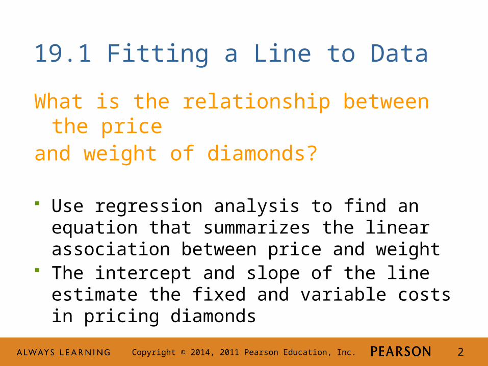
19.1 Fitting a Line to Data
What is the relationship between the price and weight of diamonds?
Use regression analysis to find an equation that summarizes the linear association between price and weight
The intercept and slope of the line estimate the fixed and variable costs in pricing diamonds

Copyright © 2014, 2011 Pearson Education, Inc. 3
19.1 Fitting a Line to Data
Consider Two Questions about Diamonds:
What’s the average price of diamonds that weigh 0.4 carat?
How much more do diamonds that weigh 0.5 carat cost?

Copyright © 2014, 2011 Pearson Education, Inc. 4
19.1 Fitting a Line to Data
Equation of a Line
Using a sample of diamonds of various weights, regression analysis produces an equation that relates weight to price.
Let y denote the response variable (price) and let x denote the explanatory (or predictor) variable (weight).

Copyright © 2014, 2011 Pearson Education, Inc. 5
19.1 Fitting a Line to Data
Scatterplot of Cost vs. Weight
Linear association is evident (r = 0.71).

Copyright © 2014, 2011 Pearson Education, Inc. 6
19.1 Fitting a Line to Data
Equation of a Line
Identify the line fit to the data by an intercept and a slope .
The equation of the line is
Estimated Cost = Weight.
xbby 10ˆ
10 bb
0b1b

Copyright © 2014, 2011 Pearson Education, Inc. 7
19.1 Fitting a Line to Data
Least Squares
Residual: vertical deviation of a point from the line ( ).
The best fitting line collectively makes the squares of residuals as small as possible (the choice of b0 and b1 minimizes the sum of the squared residuals).
yye ˆ

Copyright © 2014, 2011 Pearson Education, Inc. 8
19.1 Fitting a Line to Data
Residuals – Vertical Deviation (+ or -)

Copyright © 2014, 2011 Pearson Education, Inc. 9
19.1 Fitting a Line to Data
Least Squares Regression
x
y
s
srb 1
xbyb 10

Copyright © 2014, 2011 Pearson Education, Inc. 10
19.2 Interpreting the Fitted Line
Diamond Example
The least squares regression equation for relating diamond prices to weight is
Estimated Cost = 15 + 2,697 Weight
Copyright © 2014, 2011 Pearson Education, Inc. 11
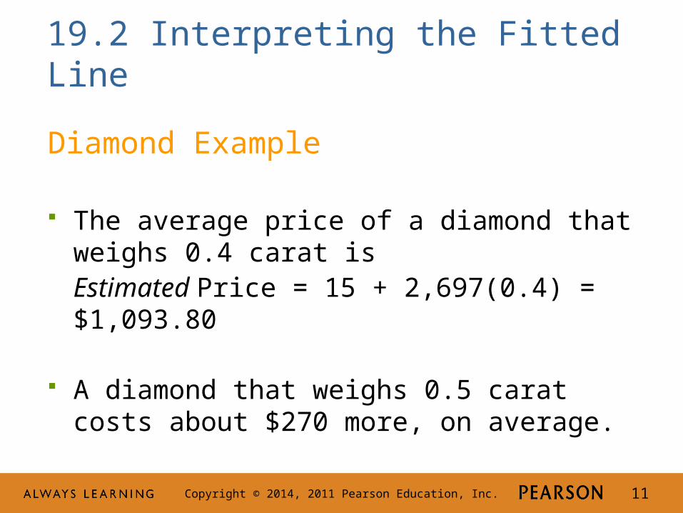
19.2 Interpreting the Fitted Line
Diamond Example
The average price of a diamond that weighs 0.4 carat is Estimated Price = 15 + 2,697(0.4) = $1,093.80
A diamond that weighs 0.5 carat costs about $270 more, on average.

Copyright © 2014, 2011 Pearson Education, Inc. 12
19.2 Interpreting the Fitted Line
Diamond Example

Copyright © 2014, 2011 Pearson Education, Inc. 13
19.2 Interpreting the Fitted Line
Interpreting the Intercept
The intercept is the portion of y that is present for all values of x (i.e., fixed cost, $15, per diamond).
The intercept estimates the average response when x = 0 (where the line crosses the y axis).

Copyright © 2014, 2011 Pearson Education, Inc. 14
19.2 Interpreting the Fitted Line
Interpreting the Intercept
Unless the range of x values includes zero, b0 will
be an extrapolation.

Copyright © 2014, 2011 Pearson Education, Inc. 15
19.2 Interpreting the Fitted Line
Interpreting the Slope
The slope estimates the marginal cost used to find the variable cost (i.e., marginal cost is $2,697 per carat).
While tempting, it is not correct to describe the slope as the change in y caused by changing x.

Copyright © 2014, 2011 Pearson Education, Inc. 16
4M Example 19.1: ESTIMATING CONSUMPTION
Motivation
A utility company that sells natural gas in the Philadelphia area needs to estimate how much is used in homes in which their meters cannot be read.
Copyright © 2014, 2011 Pearson Education, Inc. 17
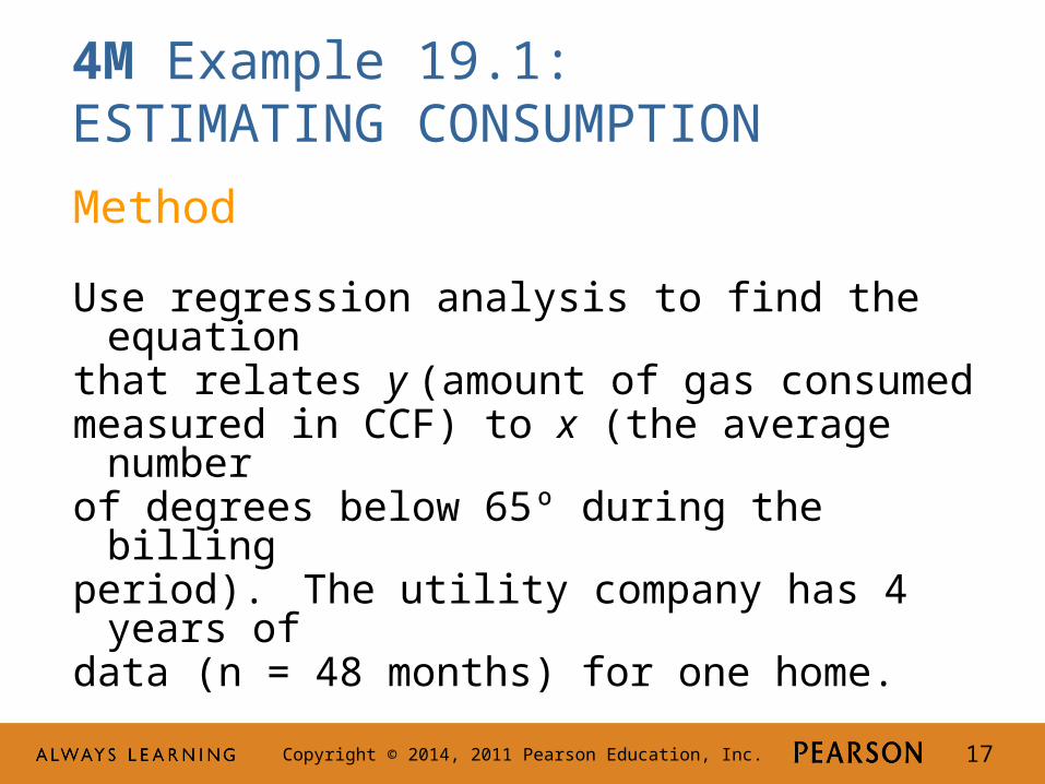
4M Example 19.1: ESTIMATING CONSUMPTION
Method
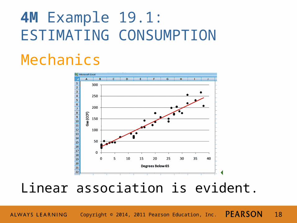
Use regression analysis to find the equation that relates y (amount of gas consumed measured in CCF) to x (the average number of degrees below 65º during the billing period). The utility company has 4 years of data (n = 48 months) for one home.
Copyright © 2014, 2011 Pearson Education, Inc. 18
4M Example 19.1: ESTIMATING CONSUMPTION
Mechanics
Linear association is evident.

Copyright © 2014, 2011 Pearson Education, Inc. 19
4M Example 19.1: ESTIMATING CONSUMPTION
Mechanics
The fitted least squares regression line is
Estimated Gas = 26.7 + 5.7 Degrees Below 65

Copyright © 2014, 2011 Pearson Education, Inc. 20
4M Example 19.1: ESTIMATING CONSUMPTION
Message
During the summer, the home uses about 26.7 CCF of gas during the billing period. As the weather gets colder, the estimated average amount of gas consumed rises by 5.7 CCF for each additional degree below 65º.
Copyright © 2014, 2011 Pearson Education, Inc. 21
19.3 Properties of Residuals
Residuals
Show variation that remains in the data after accounting for the linear relationship defined by the fitted line.
Should be plotted against x to check for patterns.

Copyright © 2014, 2011 Pearson Education, Inc. 22
19.3 Properties of Residuals
Residual Plots
If the least squares line captures the association between x and y, then a plot of residuals versus x should stretch out horizontally with consistent vertical scatter.
Can use the visual test for association to check for the absence of a pattern.

Copyright © 2014, 2011 Pearson Education, Inc. 23
19.3 Properties of Residuals
Residual Plot for Diamond Example
There is no clear pattern. The fitted line captures the pattern that relates weight to price.

Copyright © 2014, 2011 Pearson Education, Inc. 24
19.3 Properties of Residuals
Standard Deviation of Residuals (se)
Measures how much the residuals vary around the fitted line.
Also known as standard error of the regression or the root mean squared error (RMSE).
For the diamond example, se = $145.

Copyright © 2014, 2011 Pearson Education, Inc. 25
19.3 Properties of Residuals
Standard Deviation of Residuals
Since the residuals are approximately normal, the empirical rule implies that about 95% of the prices are within $290 of the regression.

Copyright © 2014, 2011 Pearson Education, Inc. 26
19.4 Explaining Variation
Residuals Vary Less than Original Costs

Copyright © 2014, 2011 Pearson Education, Inc. 27
19.4 Explaining Variation
R-squared (r2)
Is the square of the correlation between x and y.
Is the fraction of the variation accounted for by the least squares regression line.
For the diamond example, r2 ≈ 0.5 (i.e., the fitted line explains about 50% of the variation in price).

Copyright © 2014, 2011 Pearson Education, Inc. 28
19.4 Explaining Variation
Summarizing the Fit of Line
Always report both r2 and se so others can judge how well the regression equation describes the data.

Copyright © 2014, 2011 Pearson Education, Inc. 29
19.5 Conditions for Simple Regression
Checklist
No obvious lurking variable: need to think about whether other explanatory variables might better explain the linear association between x and y.
Linear: use scatterplot to see if pattern resembles a straight line.
Random residual variation: use the residual plot to make sure no pattern exists.
Copyright © 2014, 2011 Pearson Education, Inc. 30
4M Example 19.2: LEASE COSTS
Motivation
How can a dealer anticipate the effect of age on the value of a used car? The dealer estimates that $4,000 is enough to cover the depreciation per year.
Copyright © 2014, 2011 Pearson Education, Inc. 31
4M Example 19.2: LEASE COSTS
Method
Use regression analysis to find the equation that relates y (resale value in dollars) to x (age of the car in years). The car dealer has data on the prices and age of 183 used BMWs in the 3-series from Web sites advertising certified used BMWs in 2011.
Copyright © 2014, 2011 Pearson Education, Inc. 32
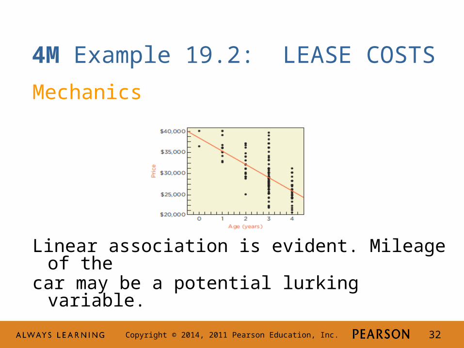
4M Example 19.2: LEASE COSTS
Mechanics
Linear association is evident. Mileage of the car may be a potential lurking variable.
Copyright © 2014, 2011 Pearson Education, Inc. 33
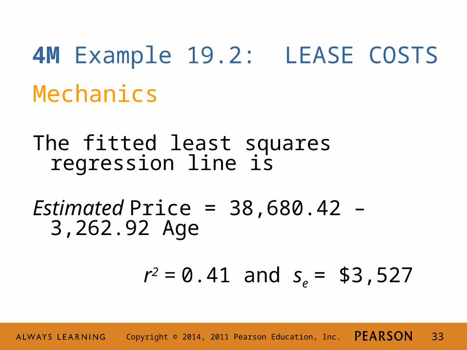
4M Example 19.2: LEASE COSTS
Mechanics
The fitted least squares regression line is
Estimated Price = 38,680.42 – 3,262.92 Age
r2 = 0.41 and se = $3,527

Copyright © 2014, 2011 Pearson Education, Inc. 34
4M Example 19.2: LEASE COSTS
Mechanics
There is more variation among residuals for cars that are 3 years old compared to other ages. Keep this in mind going forward.

Copyright © 2014, 2011 Pearson Education, Inc. 35
4M Example 19.2: LEASE COSTS
Message
The results indicate that used BMWs in the 3-series decline in resale value by $3,300 per year. The current lease price of $4,000 per year appears profitable. However, the fitted line leaves more than half of the variation unexplained. And leases longer than 4 years would require extrapolation.
Copyright © 2014, 2011 Pearson Education, Inc. 36
Best Practices
Always look at the scatterplot.
Know the substantive context of the model.
Describe the intercept and slope using units of the data.
Limit predictions to the range of observed conditions.

Copyright © 2014, 2011 Pearson Education, Inc. 37
Pitfalls
Do not assume that changing x causes changes in y.
Do not forget lurking variables.
Don’t trust summaries like r2 without looking at plots.