Embed Size (px)
Citation preview

Copyright
by
James Patrick Sutton
2007
Evaluating the Redundancy of Steel Bridges: Effect of a Bridge Haunch
on the Strength and Behavior of Shear Studs under Tensile Loading
by
James Patrick Sutton, B.S.C.E.
Thesis
Presented to the Faculty of the Graduate School of
The University of Texas at Austin
in Partial Fulfillment
of the Requirements
for the Degree of
Master of Science in Engineering
The University of Texas at Austin
May 2007
Evaluating the Redundancy of Steel Bridges: Effect of a Bridge Haunch
on the Strength and Behavior of Shear Studs under Tensile Loading
APPROVED BY SUPERVISING COMMITTEE:
Karl H. Frank
Eric B. Williamson

Dedication
To Mom and Dad for your endless love and support in everything that I do
To Molly for loving and supporting me throughout my time in Texas
To Erin, Patrick, and Mary Beth for making growing up in the Sutton house so much fun

v
Acknowledgements
First, I would like to thank Dr. Karl H. Frank for all of his help and guidance over
the course of the two years that I have been at the University of Texas. I enjoyed
learning from him and am very thankful to have had the opportunity to work with him on
this project. Also, thanks to Dr. Eric B. Williamson for his help as the co-supervisor of
this project and as the second reader of this thesis. Thanks to all the members of the
faculty, who were always willing to offer advice and help.
I would like to acknowledge my research partners, Tim Barnard, Catherine
Hovell, and Joshua Mouras. Particular thanks to Josh for the many hours that he spent
helping me with the construction, instrumentation, and testing of my specimens. I would
like to thank Omar Espinoza and Lewis Agnew as well for their help during the casting of
my test specimens. I would also like to thank all of the other graduate students that
worked at the lab over the past two years for always being around to help with homework
or research problems and for being great friends.
I would like to thank Blake Stasney, Dennis Fillip and Greg Harris for all of their
help while I worked at the lab. I would like to thank Eric Schell and Mike Wason for
their help with the setup and trouble-shooting of the data acquisition system. Finally, I
would like to thank Ella Schwartz and Barbara Howard for all their help with the
ordering of materials and supplies.
Last, but certainly not least, thanks to the people at the Texas Department of
Transportation for funding this project and for showing a genuine interest in the results of
the research.
May 4, 2007
vi
Abstract
Evaluating the Redundancy of Steel Bridges: Effect of a Bridge Haunch
on the Strength and Behavior of Shear Studs under Tensile Loading
James Patrick Sutton, M.S.E.
The University of Texas at Austin, 2007
Supervisor: Karl H. Frank
AASHTO defines a fracture critical member (FCM) as a component in tension
whose failure is expected to result in the collapse of the bridge. Bridges with FCMs must
be inspected more frequently for this reason, which can lead to greater cost during the life
of the bridge and a general reluctance to design new bridges with FCMs. However,
evidence has shown that certain bridges with FCMs have redundant load paths and can
withstand a fracture to an FCM.
There are many twin steel box girder bridges across the state of Texas, all of
which are considered to be fracture critical because it is assumed that a fracture in one
girder will initiate a total bridge collapse. In order to prevent collapse after the fracture
of one box girder, the load that had been resisted by that girder must be transferred to the
intact girder. The fractured girder will deflect so that the shear studs are loaded in
tension and the deck slab is bending in double curvature. The shear studs and deck slab
must both have the capacity to transfer the force over to the other girder.
vii
The governing failure mode for the studs loaded in tension is a concrete breakout
failure. This is a brittle failure in which the studs pull out with a large prism of concrete.
When making these calculations, it was discovered that the bridge haunch may greatly
reduce the concrete breakout strength of a single row of studs because it creates an edge
effect. In order to determine the exact effect that the bridge haunch has on the tensile
capacity of the shear studs, a series of laboratory tests were performed on bridge deck
sections with and without a haunch.
The results of the laboratory tests showed that the bridge haunch greatly reduces
the capacity of a row of studs grouped transversely across the top flange. More
importantly the specimens with a haunch exhibited no ductility at failure, which may
prevent redistribution of load during a fracture event. The specimens without a haunch
did not suffer a reduction in strength when multiple studs were grouped across the flange
width because there was no edge effect. In addition these specimens exhibited some
ductility at failure because the studs extended into the bottom reinforcement mat, which
forced the reinforcement bars to intersect the breakout failure plane.
The haunch is a necessary part of bridge construction, and despite the negative
effects it has on the tensile behavior of the studs, it cannot be eliminated. With this in
mind a series of techniques to improve the tensile behavior of the studs are
recommended. These techniques include using haunch reinforcement bars, spacing studs
longitudinally rather than grouping the studs transversely across the flange width, using
longer studs, and developing a reduced diameter shear stud that will make yielding of the
studs the governing failure mode. Yielding of the studs is the ideal failure mode because
it would allow for the most redistribution of load during a fracture event.
viii
Table of Contents
List of Tables ........................................................................................................ xii
List of Figures ...................................................................................................... xiii
CHAPTER 1 1
Introduction and Background ..................................................................................1 1.1 Fracture Critical Bridges...........................................................................1 1.2 FSEL Fracture Critical Bridge Test ..........................................................3 1.3 Analysis of Bridge Components ...............................................................5
1.3.1 Introduction...................................................................................5 1.3.2 Load Path ......................................................................................5 1.3.3 Analysis of Shear Studs ................................................................7 1.3.4 Analysis of Deck Slab...................................................................7 1.3.5 Analysis of Composite Section...................................................10 1.3.6 Summary .....................................................................................11
CHAPTER 2 12
Strength of Concrete Anchors under Tensile Loading ..........................................12 2.1 Introduction.............................................................................................12 2.2 Tensile Strength of Concrete Anchors....................................................12
2.2.1 Overview: ACI 318 Appendix D – Anchoring to Concrete .......12 2.2.2 Steel Strength ..............................................................................14 2.2.3 Concrete Breakout Strength........................................................14 2.2.4 Pullout Strength ..........................................................................20 2.2.5 Concrete Side-Face Blowout Strength........................................20
2.3 Capacity of a Row of Studs on the FSEL Test Bridge ...........................21 2.4 Summary .................................................................................................25
ix
CHAPTER 3 26
Testing Program.....................................................................................................26 3.1 Introduction.............................................................................................26 3.2 Test Specimens .......................................................................................27
3.2.1 Specimen Details ........................................................................27 3.2.2 Stud Welding ..............................................................................33 3.2.3 Formwork....................................................................................33 3.2.4 Concrete Mix ..............................................................................34
3.3 Test Setup................................................................................................35 3.4 Instrumentation .......................................................................................36
3.4.1 Shear Studs..................................................................................36 3.4.2 Reinforcing Steel ........................................................................37 3.4.3 Load and Displacement...............................................................39
3.5 Testing Procedure ...................................................................................40
CHAPTER 4 42
Test Results............................................................................................................42 4.1 General Comments..................................................................................42 4.2 Capacity ..................................................................................................43 4.3 Behavior at Failure..................................................................................44
4.3.1 Specimens with a Haunch...........................................................44 4.3.2 Specimens with No Haunch........................................................47
4.4 Stud Gage Data .......................................................................................49 4.4.1 Analysis of Data..........................................................................49 4.4.2 Specimens with a Haunch...........................................................50 4.4.3 Specimens with No Haunch........................................................53
4.5 Reinforcing Steel Gage Data ..................................................................56 4.5.1 Concrete Slab – Cracking, Yielding, and Ultimate Loads..........56 4.5.2 Specimens with a Haunch...........................................................60 4.5.3 Specimens with No Haunch........................................................63
4.6 Slab Deflection........................................................................................66
x
4.7 Concrete Cylinder Tests..........................................................................68
CHAPTER 5 69
Analysis and Discussion of Test Results ...............................................................69 5.1 Predicted Capacities versus Test Results................................................69 5.2 Evaluation of Current Shear Connector Detail .......................................77
5.2.1 Introduction.................................................................................77 5.2.2 Capacity ......................................................................................77 5.2.3 Ductility ......................................................................................77 5.2.4 Efficiency....................................................................................79 5.2.5 Summary .....................................................................................80
5.3 Possible Techniques to Improve Shear Connector Detail.......................81 5.3.1 General Comments......................................................................81 5.3.2 Haunch Reinforcement ...............................................................81 5.3.3 Longitudinal Spacing of Studs....................................................83 5.3.4 Longer Studs ...............................................................................85 5.3.5 Combination of Longer Studs and Longitudinal Spacing...........87 5.3.6 Reduction of Stud Diameter........................................................89 5.3.7 Summary .....................................................................................93
CHAPTER 6 94
Conclusions and Recommendations ......................................................................94 6.1 Summary of Objectives...........................................................................94 6.2 Conclusions.............................................................................................94 6.3 Recommendations and Future Work ......................................................97

xi
APPENDIX A 99
Analysis of Bridge Components ............................................................................99
APPENDIX B 109
FSEL Bridge Deck Details and TxDOT Stud Detail ...........................................109
APPENDIX C 113
Complete Test Specimen Details .........................................................................113
APPENDIX D 119
Test Specimens – Cracking, Yield and Ultimate Load........................................119
APPENDIX E 124
Predicted Tensile Capacity of Test Specimens....................................................124
APPENDIX F 131
Mill Test Report for Studs used in Test Specimens.............................................131
REFERENCES 132
VITA 133
xii
List of Tables
Table 2.1: Estimated tensile capacities for a single stud and a row of three studs on
the FSEL test bridge (fc’ = 4,000 psi; 7/8-in. diameter x 5-in. long studs;
futa = 60,000 psi)................................................................................24
Table 3.1: Specimen identification and details ......................................................30
Table 4.1: Testing order.........................................................................................42
Table 4.2: Maximum load resisted by each specimen ...........................................43
Table 4.3: Stud gage data at maximum load for specimens with a 3-in. haunch...50
Table 4.4: Stud gage data at maximum load for specimens with no haunch.........54
Table 4.5: Concrete cylinder compression tests ....................................................68
Table 5.1: Calculation of predicted capacities (fc’ = 6,000 psi).............................72
Table 5.2: Experimental results versus nominal capacity from ACI design equations
...........................................................................................................73
Table 5.3: Percent difference assuming no cracking in specimens with a 3-in. haunch
...........................................................................................................74
Table 5.4: Cross-over point for a single 7/8-in. diameter stud with no edge or group
effects in various concrete compressive strengths ............................89
xiii
List of Figures
Figure 1.1: Collapse of Silver Bridge (Connor, Dexter, and Mahmoud, 2005) ......1
Figure 1.2: Full-depth fracture of the I-79 two girder bridge at Neville Island in
Pittsburgh, PA (Connor, Dexter, and Mahmoud, 2005) .....................2
Figure 1.3: Cross-section of FSEL test bridge.........................................................4
Figure 1.4: Assumed deflected shape at point of girder fracture.............................6
Figure 1.5: Bending moment in deck slab at ultimate state.....................................8
Figure 1.6: Composite section of non-fractured girder..........................................10
Figure 2.1: FSEL test bridge shear stud – 7/8-in. diameter x 5-in. long................13
Figure 2.2: Failure modes for anchors loaded in tension (ACI 318-05)................13
Figure 2.3: Tensile breakout shape as idealized by: (a) CCD method (b) 45° cone
method (Shirvani, Klingner, and Graves III, 2004) ..........................15
Figure 2.4: Multiple studs behaving as a group – (a) projected failure area (b) section
through failure prism; multiple studs behaving independently – (c)
projected failure areas (d) section through failure prisms ................18
Figure 2.5: Edge reduction (c < 1.5hef) – (a) section through failure prism (b)
projected failure area.........................................................................19
Figure 2.6: Shear stud detail for FSEL test bridge.................................................22
Figure 2.7: Concrete breakout prism following 35° angle.....................................23
Figure 3.1: Bridge slab in double curvature...........................................................27
Figure 3.2: Transverse and longitudinal directions of test specimens ...................28
Figure 3.3: Details for specimens with no haunch.................................................31
Figure 3.4: Details for specimens with 3-in. haunch .............................................32
Figure 3.5: (a) Stud welding; (b) bend over test ....................................................33
xiv
Figure 3.6: Formwork for specimens with (a) no haunch (b) 3-in. haunch ...........34
Figure 3.7: Test setup.............................................................................................35
Figure 3.8: (a) Stud gage installation.....................................................................36
Figure 3.8 (cont.): (b) shear stud after gage installation; (c) drawing of typical stud
gage placement..................................................................................37
Figure 3.9: Instrumentation of reinforcing steel ....................................................38
Figure 3.10: Labeling of gages on steel reinforcing bars.......................................38
Figure 3.11: Attachment of load cell .....................................................................39
Figure 3.12: Linear potentiometer measuring separation between the slab and WT.
...........................................................................................................40
Figure 3.13: Test setup, hydraulic setup and data acquisition system...................41
Figure 4.1: Specimen 3-1b – Applied load versus stud pullout deflection............45
Figure 4.2: Initial cracking in specimen with a 3-in. haunch.................................46
Figure 4.3: Specimens with a 3-in. haunch – (a) Center crack at failure; (b) horizontal
cracking across top of haunch; (c) complete separation of haunch ..47
Figure 4.4: Specimen 0-3b – Applied load versus stud pullout deflection............48
Figure 4.5: Specimens with no haunch – (a) Increased flexural cracking; (b) breakout
prism cracking as seen from underside of specimen; (c) formation of
breakout prism ..................................................................................49
Figure 4.6: Tensile resistance provided by shear stud ...........................................51
Figure 4.7: Specimen 3-2b – Applied load versus calculated force in the shear studs
...........................................................................................................52
Figure 4.8: Specimen 3-3b – Applied load versus calculated force in the shear studs
...........................................................................................................53
xv
Figure 4.9: Applied load versus calculated force in the shear studs – (a) Specimen 0-
3a; (b) Specimen 0-3b.......................................................................55
Figure 4.10: Assumed location of neutral axis at yield of bottom reinforcement .58
Figure 4.11: Strain and stress profiles at point of yield .........................................59
Figure 4.12: Strain and stress profile at ultimate ...................................................60
Figure 4.13: Specimen 3-2b – Reinforcing steel load versus strain at the (a) mid-span
location (b) quarter-span location .....................................................62
Figure 4.14: Specimen 0-2a – Mid-span reinforcing steel load versus strain........64
Figure 4.15: Specimen 0-3a – Mid-span reinforcing steel load versus strain........65
Figure 4.16: Specimen 0-3a – Quarter-span reinforcing steel load versus strain ..66
Figure 4.17: Specimen 3-3a – Typical load versus top of slab deflection plot......67
Figure 5.1: Assumed projected concrete failure area of studs for specimens with a 3-
in. haunch and (a) one stud, (b) two studs, and (c) three studs.........71
Figure 5.2: Assumed projected concrete failure area of studs for specimens with no
haunch and (a) one stud, (b) two studs, and (c) three studs ..............72
Figure 5.3: Specimen with 3-in. haunch – no flexural cracking in haunch ...........74
Figure 5.4: Deck transverse direction – (a) assumed breakout failure; (b) actual
breakout failure .................................................................................75
Figure 5.5: Deck longitudinal direction – (a) assumed breakout failure; (b) actual
breakout failure .................................................................................75
Figure 5.6: (a) Assumed projected failure area; (b) actual failure area .................76
Figure 5.7: Complete haunch separation as seen from (a) the side view and (b)
underneath the specimen...................................................................78
xvi
Figure 5.8: (a) Drawing and (b) photograph showing the center transverse bars
running through the concrete failure prism for a specimen with no
haunch ...............................................................................................79
Figure 5.9: Haunch reinforcement to improve ductility (a) cross-section (b) plan view
...........................................................................................................82
Figure 5.10: Load versus stud pullout for (a) current detail and (b) reinforced haunch
detail..................................................................................................83
Figure 5.11: Longitudinal spacing of shear studs ..................................................84
Figure 5.12: (a) 5-in. long studs with no haunch; (b) 8-in. long studs with 3-in.
haunch ...............................................................................................86
Figure 5.13: Potential concrete breakout failure prism for longer studs................86
Figure 5.14: Tensile capacity versus effective height for a single 7/8-in. diameter stud
embedded in 4,000 psi concrete........................................................88
Figure 5.15: Reduced diameter shear stud.............................................................92
Figure 5.16: Stud under shear and bending ...........................................................92
Figure A.1: Truck load distribution, shear diagram, and moment diagram.........100
Figure A.2: Deck slab – 1-ft wide section ...........................................................102
Figure A.3: Strain and stress profiles at positive moment capacity.....................102
Figure A.4: Strain and stress profiles at negative moment capacity....................103
Figure A.5: Assumed bending moment in deck slab at ultimate state.................105
Figure A.6: Composite section ............................................................................106
Figure A.7: Plastic neutral axis location ..............................................................107
Figure B.1: FSEL bridge deck – typical transverse section.................................109
Figure B.2: FSEL bridge deck – plan view..........................................................110
Figure B.3: Notes for FSEL bridge deck drawings (Fig. B.1-B.2)......................111
xvii
Figure B.4: TxDOT typical stud connector detail for three studs (TxDOT Bridge
Standard Drawings: Miscellaneous Details (Steel Girders and Beams),
2006) ...............................................................................................112
Figure C.1: Specimen 0-1 (a,b)............................................................................113
Figure C.2: Specimen 0-2 (a,b)............................................................................114
Figure C.3: Specimen 0-3 (a.b)............................................................................115
Figure C.4: Specimen 3-1 (a,b)............................................................................116
Figure C.5: Specimen 3-2 (a,b)............................................................................117
Figure C.6: Specimen 3-3 (a,b) ...........................................................................118
Figure D.1: Test specimen – slab cross section ...................................................119
Figure D.2: Assumed location of neutral axis at yield load.................................120
Figure D.3: Assumed strain and stress profile at yielding ...................................121
Figure D.4: Assumed strain and stress profiles at ultimate moment capacity .....122
Figure E.1: Stud details for specimens with no haunch.......................................124
Figure E.2: Concrete breakout – projected failure areas for specimens with no haunch
(ANc) ................................................................................................125
Figure E.3: Stud details for specimens with a 3 in. haunch.................................128
Figure E.4: Concrete breakout – projected failure areas for specimens with a 3 in.
haunch (ANc) ....................................................................................128
Figure F.1: Shear stud mill test report .................................................................131
1
CHAPTER 1
Introduction and Background
1.1 FRACTURE CRITICAL BRIDGES
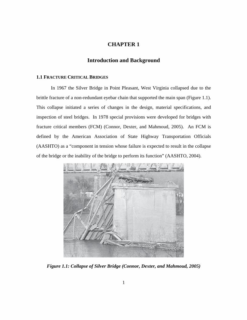
In 1967 the Silver Bridge in Point Pleasant, West Virginia collapsed due to the
brittle fracture of a non-redundant eyebar chain that supported the main span (Figure 1.1).
This collapse initiated a series of changes in the design, material specifications, and
inspection of steel bridges. In 1978 special provisions were developed for bridges with
fracture critical members (FCM) (Connor, Dexter, and Mahmoud, 2005). An FCM is
defined by the American Association of State Highway Transportation Officials
(AASHTO) as a “component in tension whose failure is expected to result in the collapse
of the bridge or the inability of the bridge to perform its function” (AASHTO, 2004).
Figure 1.1: Collapse of Silver Bridge (Connor, Dexter, and Mahmoud, 2005)
2
Fracture critical bridges (FCB), or bridges with an FCM, are required to be
inspected more frequently than a bridge that is considered non-fracture critical. The cost
of inspection during the life of an FCB can typically be two to five times greater than a
bridge without FCMs (Connor, Dexter, and Mahmoud, 2005). The increased cost
associated with FCBs has led to fewer new FCBs being designed even in situations when
an FCB may be a more effective solution.
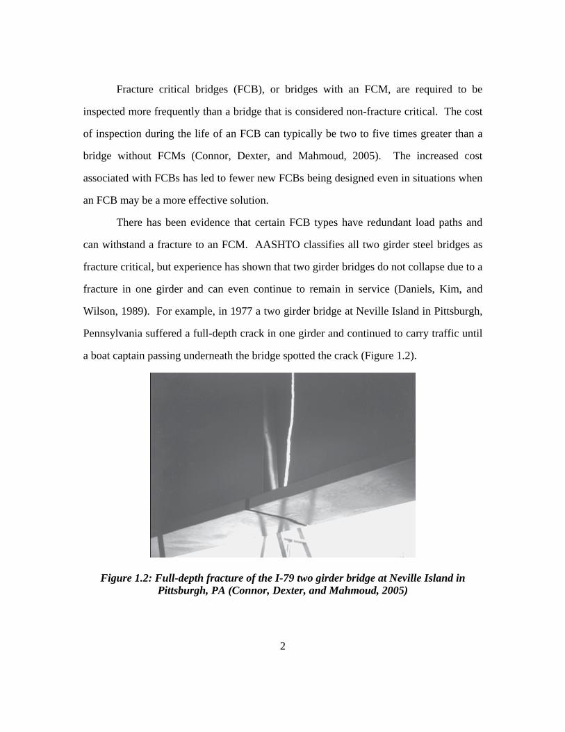
There has been evidence that certain FCB types have redundant load paths and
can withstand a fracture to an FCM. AASHTO classifies all two girder steel bridges as
fracture critical, but experience has shown that two girder bridges do not collapse due to a
fracture in one girder and can even continue to remain in service (Daniels, Kim, and
Wilson, 1989). For example, in 1977 a two girder bridge at Neville Island in Pittsburgh,
Pennsylvania suffered a full-depth crack in one girder and continued to carry traffic until
a boat captain passing underneath the bridge spotted the crack (Figure 1.2).
Figure 1.2: Full-depth fracture of the I-79 two girder bridge at Neville Island in Pittsburgh, PA (Connor, Dexter, and Mahmoud, 2005)
3
Current bridge specifications assume that two girder bridges are fracture critical
because they assume that the structural components of a bridge behave independently,
but in reality these components interact with each other to form one structural system
(Ghosn and Moses, 1998). In the case of two girder bridges, other components such as
the deck slab can provide a redundant load path and prevent collapse when one girder
experiences a fracture (Connor, Dexter, and Mahmoud, 2005).
1.2 FSEL FRACTURE CRITICAL BRIDGE TEST
The opportunity to perform a full-scale fracture test arose when the Texas
Department of Transportation (TxDOT) was removing a 120-ft simple span twin steel
trapezoidal box girder bridge segment along Interstate Highway 10 in Houston. There
are many twin steel box girder bridges in the state of Texas, all of which are considered
to be FCBs. The inspection of box girder bridges is particularly difficult and expensive
because it requires the inspector to be inside of the box girder. The goal of this fracture
test was to learn about the load transfer that takes place during a fracture event and to use
that information to help calibrate an analytical model that can predict the behavior of twin
girder FCBs in a fracture event.
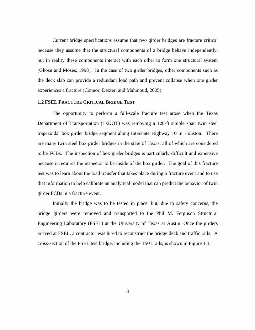
Initially the bridge was to be tested in place, but, due to safety concerns, the
bridge girders were removed and transported to the Phil M. Ferguson Structural
Engineering Laboratory (FSEL) at the University of Texas at Austin. Once the girders
arrived at FSEL, a contractor was hired to reconstruct the bridge deck and traffic rails. A
cross-section of the FSEL test bridge, including the T501 rails, is shown in Figure 1.3.
4
12'
23' - 4"
6'6' 6'
4' - 9"
Figure 1.3: Cross-section of FSEL test bridge
After the bridge had been reconstructed in accordance with TxDOT standard
practices, a fracture test was performed on the bridge. During the test, the bridge was
loaded with the equivalent of a 76-kip truck. The fracture was simulated by cutting the
bottom flange of the exterior girder at the mid-span location. A linear-shaped charge was
used to cut the flange to simulate the dynamic fracture of the flange. The charge cut
completely through the tension flange of the girder, but the fracture did not propagate up
the girder webs. The bridge behaved extremely well during the test, and the fractured
girder deflected only an additional 1/4 in. after the fracture of the flange.
Unfortunately, there was not much evidence of load transfer to the other girder
because the load carried by the fractured flange was simply resisted by the webs in the
area of the fracture. A future test is planned to propagate the existing crack up the webs
in order to determine how the load is transferred from the fractured girder to the non-
fractured girder and to determine if the bridge can withstand a full depth fracture without
collapse.
5
1.3 ANALYSIS OF BRIDGE COMPONENTS
1.3.1 Introduction
Currently, the best way to model system behavior is through the use of detailed
analytical models such as finite element programs. While these models may produce the
most accurate results, they also require a substantial amount of work and time to be
developed and to be run. It would be beneficial for designers or bridge owners to have a
simple set of analytical procedures that can be checked before developing a complex
finite element model. If these simple analyses show that a bridge might have adequate
redundancy, a more detailed analysis can then be developed to confirm that the system
can withstand a fracture to an FCM. However, if the simple analyses show that the
bridge cannot withstand a fracture to an FCM, then the time and money that would have
been spent on a more detailed model can be saved.
A set of simple calculations was developed to predict the behavior of the FSEL
test bridge during the fracture test. These analyses focused on the individual components
of the bridge that would be required to provide an alternate load path after the fracture of
one girder – namely the shear studs, deck slab, and remaining girder. In each case
specific assumptions were made in order to simplify the analysis. Therefore, these
analyses do not capture the exact behavior of the system during a fracture event. Rather,
they are meant to be used as an initial check prior to making the decision to develop a
detailed finite element model.
1.3.2 Load Path
After a fracture occurs in the tension flange of one of the girders and propagates
up the webs, it is assumed that the girder will no longer be able to resist load. The
fracture at mid-span can be compared to placing a hinge in the girder. A simply
6
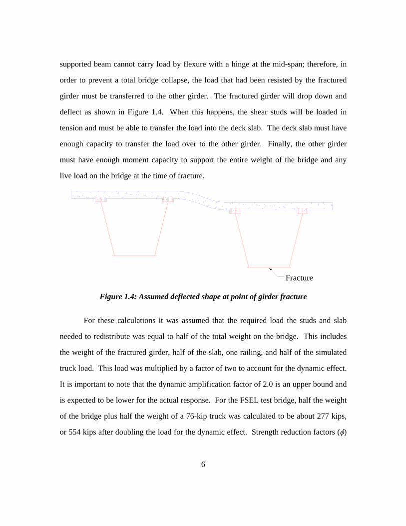
supported beam cannot carry load by flexure with a hinge at the mid-span; therefore, in
order to prevent a total bridge collapse, the load that had been resisted by the fractured
girder must be transferred to the other girder. The fractured girder will drop down and
deflect as shown in Figure 1.4. When this happens, the shear studs will be loaded in
tension and must be able to transfer the load into the deck slab. The deck slab must have
enough capacity to transfer the load over to the other girder. Finally, the other girder
must have enough moment capacity to support the entire weight of the bridge and any
live load on the bridge at the time of fracture.
Fracture
Figure 1.4: Assumed deflected shape at point of girder fracture
For these calculations it was assumed that the required load the studs and slab
needed to redistribute was equal to half of the total weight on the bridge. This includes
the weight of the fractured girder, half of the slab, one railing, and half of the simulated
truck load. This load was multiplied by a factor of two to account for the dynamic effect.
It is important to note that the dynamic amplification factor of 2.0 is an upper bound and
is expected to be lower for the actual response. For the FSEL test bridge, half the weight
of the bridge plus half the weight of a 76-kip truck was calculated to be about 277 kips,
or 554 kips after doubling the load for the dynamic effect. Strength reduction factors (φ)
7
were not applied to any of these calculations. Refer to Appendix A for the calculation
details. The concepts used to make these calculations are presented here.
1.3.3 Analysis of Shear Studs
The first components of the bridge system that must be able to transfer the load
from the fractured girder to the intact girder are the shear studs that connect the girder to
the deck slab. In order to simplify the calculations, it was assumed that the studs would
be under tension only. The equations from Appendix D of the ACI 318 Building Code
were used to calculate the tensile capacity of a single row of studs. After the capacity of
a single row of three studs was calculated, the number of rows needed to resist the 554-
kip force was determined. This calculation assumes that the studs can perform in a
ductile manner and redistribute the force along the length of the girder.
The calculation of the tensile capacity of anchors in concrete, the predicted tensile
capacity of a row of shear studs on the FSEL test bridge, and the percentage of the span
length required to distribute the 554-kip force are discussed in detail in Chapter 2.
1.3.4 Analysis of Deck Slab
Assuming that the shear studs are able to transfer load into the deck slab, the deck
slab must then be able to transfer the load across to the other box girder. In this analysis
two criteria were checked for the deck slab. The first was the flexural capacity of the
slab, and the second was the shear capacity of the slab. In each case the capacity of a 1-ft
wide section of the deck slab was calculated. Then the percentage of the total span length
needed to distribute the required force during a fracture event was determined. Refer to
Appendix A for all calculations associated with the deck slab capacity and distribution of
the 554-kip force.
8
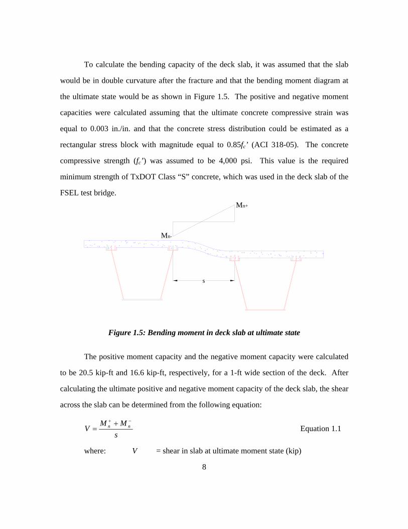
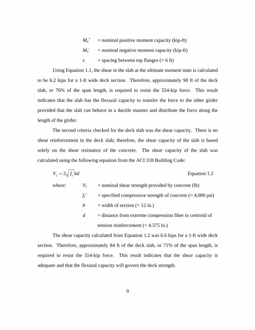
To calculate the bending capacity of the deck slab, it was assumed that the slab
would be in double curvature after the fracture and that the bending moment diagram at
the ultimate state would be as shown in Figure 1.5. The positive and negative moment
capacities were calculated assuming that the ultimate concrete compressive strain was
equal to 0.003 in./in. and that the concrete stress distribution could be estimated as a
rectangular stress block with magnitude equal to 0.85fc’ (ACI 318-05). The concrete
compressive strength (fc’) was assumed to be 4,000 psi. This value is the required
minimum strength of TxDOT Class “S” concrete, which was used in the deck slab of the
FSEL test bridge. Mn+
Mn-
s
Figure 1.5: Bending moment in deck slab at ultimate state
The positive moment capacity and the negative moment capacity were calculated
to be 20.5 kip-ft and 16.6 kip-ft, respectively, for a 1-ft wide section of the deck. After
calculating the ultimate positive and negative moment capacity of the deck slab, the shear
across the slab can be determined from the following equation:
sMM
V nn−+ +
= Equation 1.1
where: V = shear in slab at ultimate moment state (kip)
9
Mn+ = nominal positive moment capacity (kip-ft)
Mn- = nominal negative moment capacity (kip-ft)
s = spacing between top flanges (= 6 ft)
Using Equation 1.1, the shear in the slab at the ultimate moment state is calculated
to be 6.2 kips for a 1-ft wide deck section. Therefore, approximately 90 ft of the deck
slab, or 76% of the span length, is required to resist the 554-kip force. This result
indicates that the slab has the flexural capacity to transfer the force to the other girder
provided that the slab can behave in a ductile manner and distribute the force along the
length of the girder.
The second criteria checked for the deck slab was the shear capacity. There is no
shear reinforcement in the deck slab; therefore, the shear capacity of the slab is based
solely on the shear resistance of the concrete. The shear capacity of the slab was
calculated using the following equation from the ACI 318 Building Code:
bdfV cc'2= Equation 1.2
where: Vc = nominal shear strength provided by concrete (lb)
fc' = specified compressive strength of concrete (= 4,000 psi)
b = width of section (= 12 in.)
d = distance from extreme compression fiber to centroid of
tension reinforcement (= 4.375 in.)
The shear capacity calculated from Equation 1.2 was 6.6 kips for a 1-ft wide deck
section. Therefore, approximately 84 ft of the deck slab, or 71% of the span length, is
required to resist the 554-kip force. This result indicates that the shear capacity is
adequate and that the flexural capacity will govern the deck strength.
10
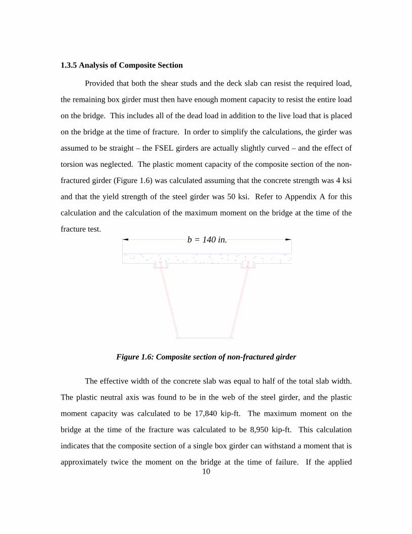
1.3.5 Analysis of Composite Section
Provided that both the shear studs and the deck slab can resist the required load,
the remaining box girder must then have enough moment capacity to resist the entire load
on the bridge. This includes all of the dead load in addition to the live load that is placed
on the bridge at the time of fracture. In order to simplify the calculations, the girder was
assumed to be straight – the FSEL girders are actually slightly curved – and the effect of
torsion was neglected. The plastic moment capacity of the composite section of the non-
fractured girder (Figure 1.6) was calculated assuming that the concrete strength was 4 ksi
and that the yield strength of the steel girder was 50 ksi. Refer to Appendix A for this
calculation and the calculation of the maximum moment on the bridge at the time of the
fracture test. b = 140 in.
Figure 1.6: Composite section of non-fractured girder
The effective width of the concrete slab was equal to half of the total slab width.
The plastic neutral axis was found to be in the web of the steel girder, and the plastic
moment capacity was calculated to be 17,840 kip-ft. The maximum moment on the
bridge at the time of the fracture was calculated to be 8,950 kip-ft. This calculation
indicates that the composite section of a single box girder can withstand a moment that is
approximately twice the moment on the bridge at the time of failure. If the applied
11
moment is multiplied by two for the dynamic effect, then the remaining girder has
exactly enough reserve capacity to support the entire weight of the bridge. Recall that the
dynamic amplification factor of 2.0 is an upper bound and is expected to be lower for the
actual response.
1.3.6 Summary
The simple analysis techniques presented in this chapter have shown that the deck
slab and the remaining box girder may be able to provide a redundant load path when one
of the box girders experiences a full-depth fracture. The third component that must be
able to provide a redundant load path is the shear studs. As is discussed in Chapter 2, the
tensile capacity of the studs can be estimated using Appendix D in the ACI 318 Building
Code, but the bridge haunch and the grouping of studs across the flange width create
some uncertainty in this calculation. A series of laboratory tests were conducted in order
to determine the effect that the bridge haunch has on both the tensile capacity and the
behavior of the studs. The remainder of this thesis, beginning with Chapter 3, discusses
these laboratory tests.
12
CHAPTER 2
Strength of Concrete Anchors under Tensile Loading
2.1 INTRODUCTION
In Chapter 1, the simple analysis techniques used to determine if the FSEL test
bridge might have the redundancy to withstand a full-depth fracture to one of the box
girders were discussed. The three components of the bridge that need to resist the load in
the fractured girder were identified as the shear studs, the deck slab, and the remaining
girder. These calculations showed that the deck slab and remaining box girder may have
the ability to resist the additional load. This chapter will discuss the strength of concrete
anchors loaded in tension and will use that information to determine if the shear studs on
the FSEL test bridge can resist the required load during a fracture event.
2.2 TENSILE STRENGTH OF CONCRETE ANCHORS
2.2.1 Overview: ACI 318 Appendix D – Anchoring to Concrete
In order to calculate the tensile capacity of the shear studs, Appendix D of the
ACI 318 Building Code was referenced. This appendix provides requirements for
concrete anchors loaded in tension, shear, or a combination of tension and shear. It
covers a wide range of both cast-in-place anchors and post-installed anchors. Cast-in-
place anchors include headed bolts, headed studs, and hooked bolts. Post-installed
anchors include expansion anchors and undercut anchors. The shear studs used on a
bridge are an example of cast-in-place headed stud anchors; thus, the remainder of this
discussion will deal with the strength of headed stud anchors in tension. A drawing of
the headed stud used on the FSEL test bridge is shown in Figure 2.1. Dimensions for
13
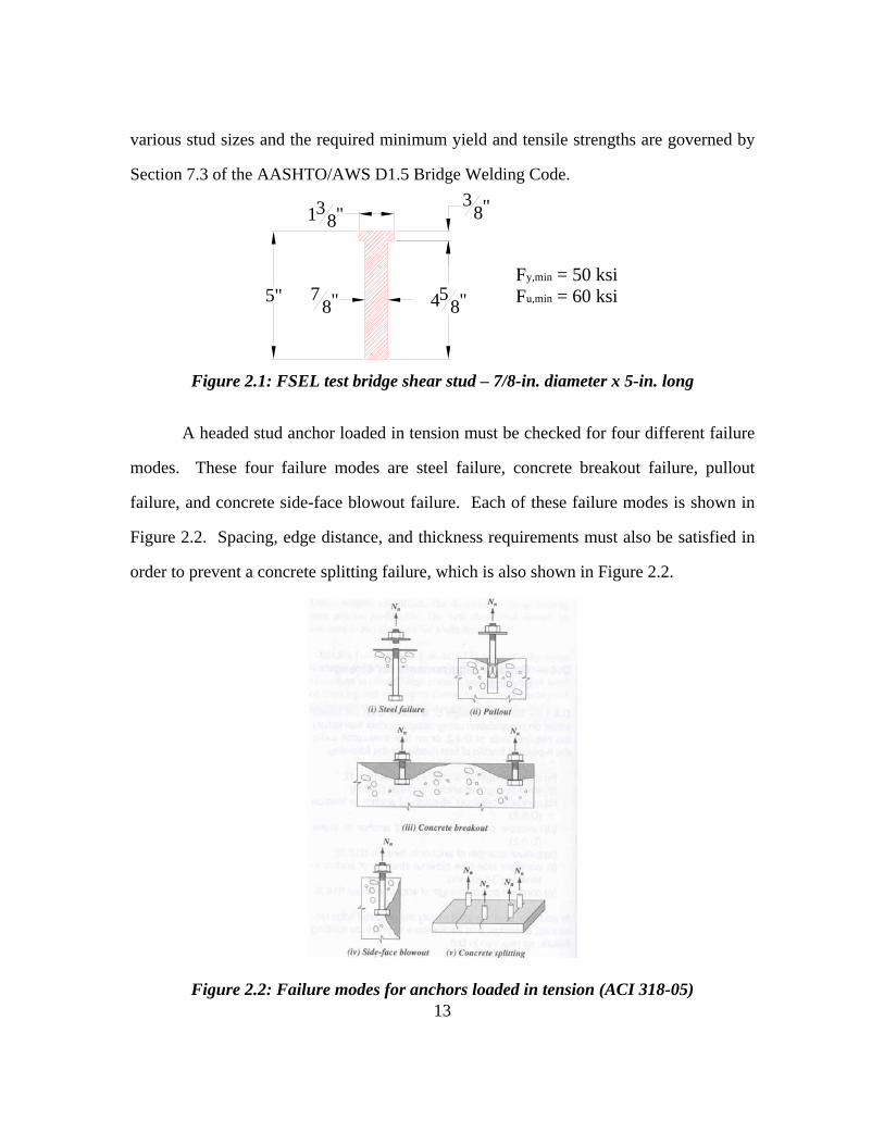
various stud sizes and the required minimum yield and tensile strengths are governed by
Section 7.3 of the AASHTO/AWS D1.5 Bridge Welding Code.
138"
38"
458"5" 7
8"Fy,min = 50 ksiFu,min = 60 ksi
Figure 2.1: FSEL test bridge shear stud – 7/8-in. diameter x 5-in. long
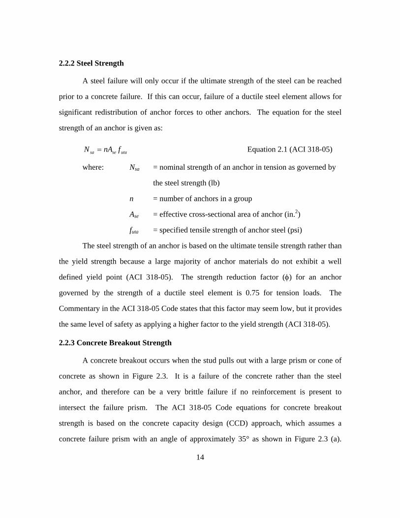
A headed stud anchor loaded in tension must be checked for four different failure
modes. These four failure modes are steel failure, concrete breakout failure, pullout
failure, and concrete side-face blowout failure. Each of these failure modes is shown in
Figure 2.2. Spacing, edge distance, and thickness requirements must also be satisfied in
order to prevent a concrete splitting failure, which is also shown in Figure 2.2.
Figure 2.2: Failure modes for anchors loaded in tension (ACI 318-05)
14
2.2.2 Steel Strength
A steel failure will only occur if the ultimate strength of the steel can be reached
prior to a concrete failure. If this can occur, failure of a ductile steel element allows for
significant redistribution of anchor forces to other anchors. The equation for the steel
strength of an anchor is given as:
utasesa fnAN = Equation 2.1 (ACI 318-05)
where: Nsa = nominal strength of an anchor in tension as governed by
the steel strength (lb)
n = number of anchors in a group
Ase = effective cross-sectional area of anchor (in.2)
futa = specified tensile strength of anchor steel (psi)
The steel strength of an anchor is based on the ultimate tensile strength rather than
the yield strength because a large majority of anchor materials do not exhibit a well
defined yield point (ACI 318-05). The strength reduction factor (φ) for an anchor
governed by the strength of a ductile steel element is 0.75 for tension loads. The
Commentary in the ACI 318-05 Code states that this factor may seem low, but it provides
the same level of safety as applying a higher factor to the yield strength (ACI 318-05).
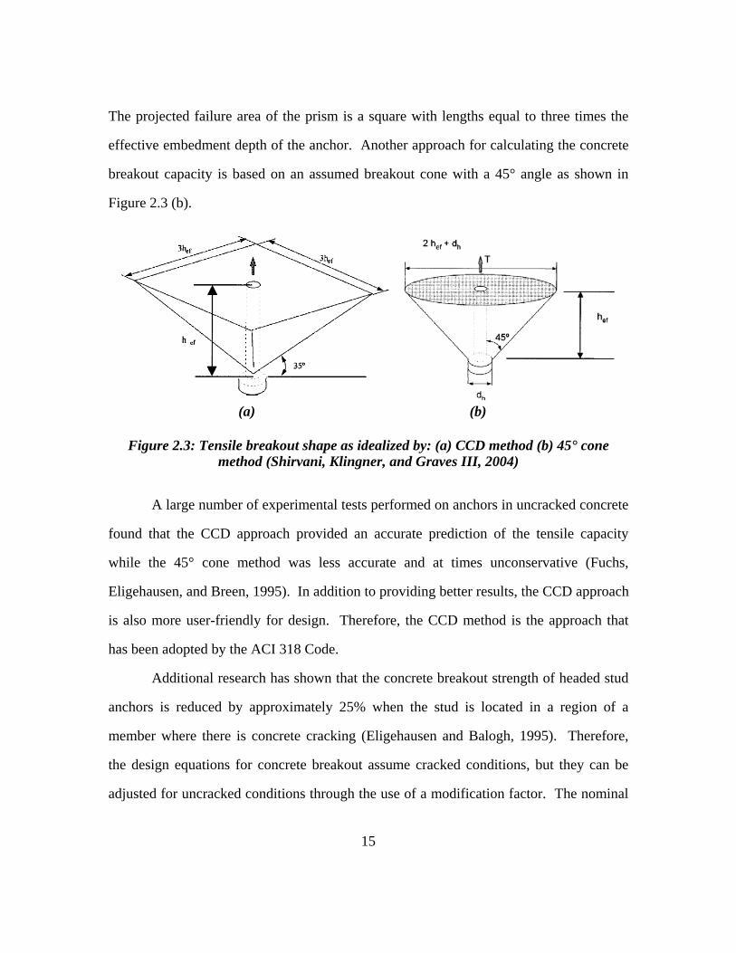
2.2.3 Concrete Breakout Strength
A concrete breakout occurs when the stud pulls out with a large prism or cone of
concrete as shown in Figure 2.3. It is a failure of the concrete rather than the steel
anchor, and therefore can be a very brittle failure if no reinforcement is present to
intersect the failure prism. The ACI 318-05 Code equations for concrete breakout
strength is based on the concrete capacity design (CCD) approach, which assumes a
concrete failure prism with an angle of approximately 35° as shown in Figure 2.3 (a).
15
The projected failure area of the prism is a square with lengths equal to three times the
effective embedment depth of the anchor. Another approach for calculating the concrete
breakout capacity is based on an assumed breakout cone with a 45° angle as shown in
Figure 2.3 (b).
(a) (b)
Figure 2.3: Tensile breakout shape as idealized by: (a) CCD method (b) 45° cone method (Shirvani, Klingner, and Graves III, 2004)
A large number of experimental tests performed on anchors in uncracked concrete
found that the CCD approach provided an accurate prediction of the tensile capacity
while the 45° cone method was less accurate and at times unconservative (Fuchs,
Eligehausen, and Breen, 1995). In addition to providing better results, the CCD approach
is also more user-friendly for design. Therefore, the CCD method is the approach that
has been adopted by the ACI 318 Code.
Additional research has shown that the concrete breakout strength of headed stud
anchors is reduced by approximately 25% when the stud is located in a region of a
member where there is concrete cracking (Eligehausen and Balogh, 1995). Therefore,
the design equations for concrete breakout assume cracked conditions, but they can be
adjusted for uncracked conditions through the use of a modification factor. The nominal
16
concrete breakout strength of an anchor or group of anchors in tension is given by the
following equations:
For a single anchor:
bNcpNcNedNco
Nccb N
AA
N ,,, ψψψ= Equation 2.2 (ACI 318-05)
For a group of anchors:
bNcpNcNedNecNco
Nccbg N
AA
N ,,,, ψψψψ= Equation 2.3 (ACI 318-05)
where: Ncb = nominal concrete breakout strength in tension of a single
anchor (lb)
Ncbg = nominal concrete breakout strength in tension of a group
of anchors (lb)
ANc = projected concrete failure area of an anchor or group of
anchors loaded in tension (in.2)
ANco = projected concrete failure area of one anchor when not
limited by edge distance or spacing (= 9hef2) (in.2)
ψec,N = modification factor to account for eccentric loading of
groups (<1.0 for eccentric loading, =1.0 for no eccentricity)
ψed,N = modification factor to account for edge distances smaller
than 1.5hef (= 1.0 if edge distance is greater than 1.5hef)
ψc,N = modification factor to account for cracking (= 1.25 if
analysis indicates no cracking; otherwise = 1.0)
ψcp,N = modification factor applicable only to post-installed
anchors (= 1.0 for cast-in anchors)
Nb = basic concrete breakout strength in tension of a single
anchor in cracked concrete (lb)
17
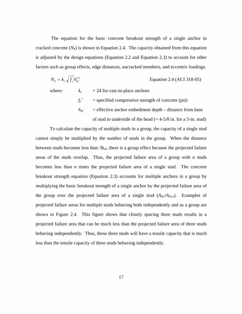
The equation for the basic concrete breakout strength of a single anchor in
cracked concrete (Nb) is shown in Equation 2.4. The capacity obtained from this equation
is adjusted by the design equations (Equation 2.2 and Equation 2.3) to account for other
factors such as group effects, edge distances, uncracked members, and eccentric loadings.
5.1'efccb hfkN = Equation 2.4 (ACI 318-05)
where: kc = 24 for cast-in-place anchors
fc’ = specified compressive strength of concrete (psi)
hef = effective anchor embedment depth – distance from base
of stud to underside of the head (= 4-5/8 in. for a 5-in. stud)
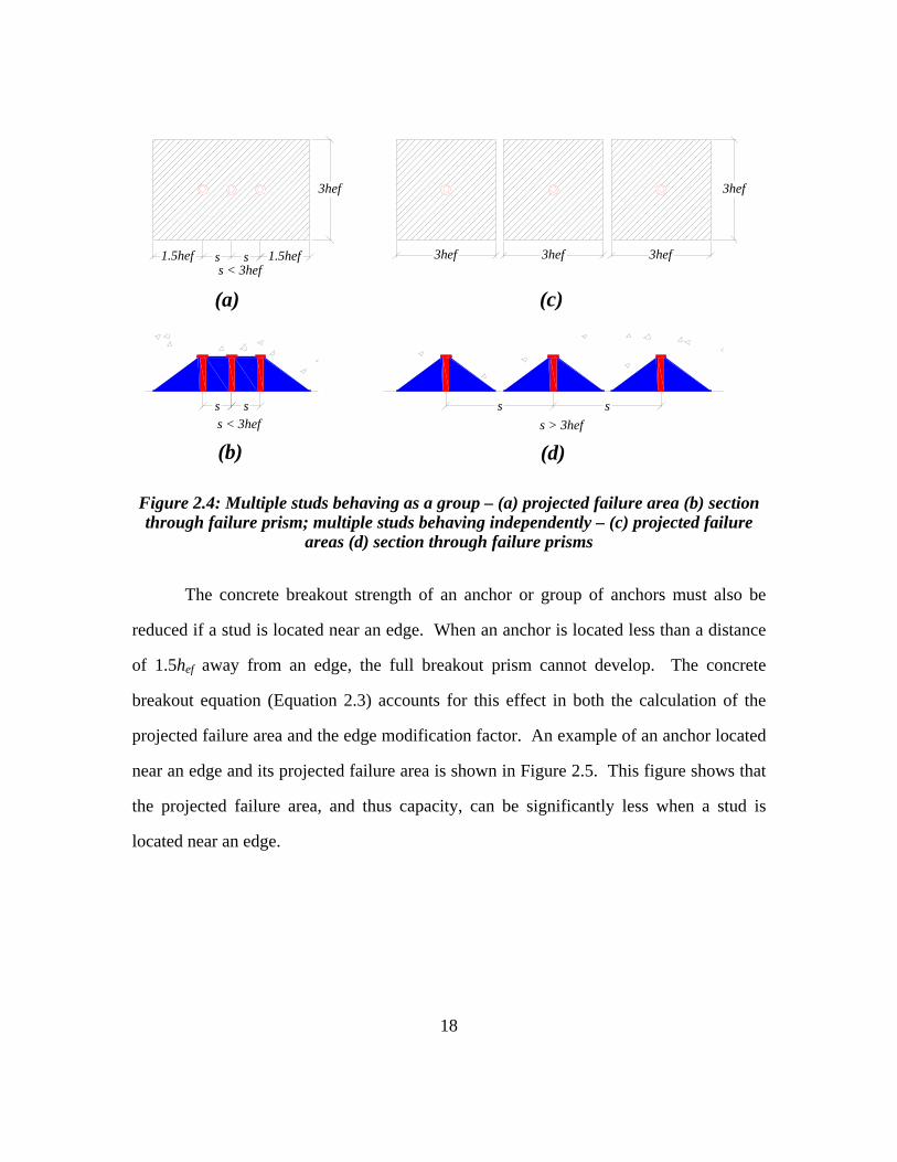
To calculate the capacity of multiple studs in a group, the capacity of a single stud
cannot simply be multiplied by the number of studs in the group. When the distance
between studs becomes less than 3hef, there is a group effect because the projected failure
areas of the studs overlap. Thus, the projected failure area of a group with n studs
becomes less than n times the projected failure area of a single stud. The concrete
breakout strength equation (Equation 2.3) accounts for multiple anchors in a group by
multiplying the basic breakout strength of a single anchor by the projected failure area of
the group over the projected failure area of a single stud (ANc/ANco). Examples of
projected failure areas for multiple studs behaving both independently and as a group are
shown in Figure 2.4. This figure shows that closely spacing three studs results in a
projected failure area that can be much less than the projected failure area of three studs
behaving independently. Thus, those three studs will have a tensile capacity that is much
less than the tensile capacity of three studs behaving independently.
18
3hef
s s1.5hef 1.5hefs < 3hef
3hef
3hef
3hef3hef
s s sss < 3hef s > 3hef
(a) (c)
(b) (d)
Figure 2.4: Multiple studs behaving as a group – (a) projected failure area (b) section through failure prism; multiple studs behaving independently – (c) projected failure
areas (d) section through failure prisms
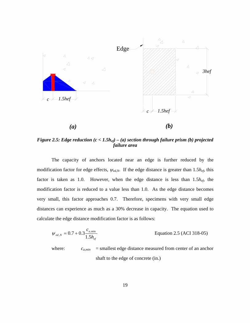
The concrete breakout strength of an anchor or group of anchors must also be
reduced if a stud is located near an edge. When an anchor is located less than a distance
of 1.5hef away from an edge, the full breakout prism cannot develop. The concrete
breakout equation (Equation 2.3) accounts for this effect in both the calculation of the
projected failure area and the edge modification factor. An example of an anchor located
near an edge and its projected failure area is shown in Figure 2.5. This figure shows that
the projected failure area, and thus capacity, can be significantly less when a stud is
located near an edge.
19
Edge
c 1.5hef
c 1.5hef
(a) (b)
3hef
Figure 2.5: Edge reduction (c < 1.5hef) – (a) section through failure prism (b) projected failure area
The capacity of anchors located near an edge is further reduced by the
modification factor for edge effects, ψed,N. If the edge distance is greater than 1.5hef, this
factor is taken as 1.0. However, when the edge distance is less than 1.5hef, the
modification factor is reduced to a value less than 1.0. As the edge distance becomes
very small, this factor approaches 0.7. Therefore, specimens with very small edge
distances can experience as much as a 30% decrease in capacity. The equation used to
calculate the edge distance modification factor is as follows:
ef
aNed h
c5.1
3.07.0 min,, +=ψ Equation 2.5 (ACI 318-05)
where: ca,min = smallest edge distance measured from center of an anchor
shaft to the edge of concrete (in.)
20
2.2.4 Pullout Strength
A pullout failure differs from a concrete breakout failure in that the stud pulls out
only the small volume of concrete directly under the stud head rather than a large prism
or cone of concrete. The equation for the pullout strength of an anchor loaded in tension
is given as:
', 8 cbrgPcpn fAN ψ= Equation 2.6 (ACI 318-05)
where: Npn = pullout strength in tension of a single anchor (lb)
ψc,P = modification factor for cracking (= 1.4 if analysis
indicates no cracking; otherwise = 1.0)
Abrg = bearing area of the head of the stud (in.2)
This equation is a function of the compressive strength of the concrete and the
bearing area of the stud head, but not the effective embedment depth. This is because the
equation corresponds to the load at which the concrete under the anchor head begins to
crush, not the load which will completely pull the anchor out of the concrete. However,
local crushing under the head greatly reduces the stiffness of the connection and is
usually the beginning of a pullout failure (ACI 318-05).
2.2.5 Concrete Side-Face Blowout Strength
A concrete side-face blowout failure can occur when an anchor with deep
embedment is located close to an edge. A concrete side-face blowout failure differs from
a concrete breakout failure because the stud does not actually pull out with a large
volume of concrete. Rather the side concrete between the stud and the edge breaks off
(Figure 2.2). If a single headed anchor is located a distance less than 0.4hef away from an
edge, the following equation must be checked:
'1160 cbrgasb fAcN = Equation 2.7 (ACI 318-05)
21
where: Nsb = side-face blowout strength of a single anchor (lb)
ca1 = distance from center of anchor shaft to the edge (in.)
When multiple studs with deep embedment are located close to an edge (ca1 <
0.4hef), the nominal concrete side-face blowout capacity is given as:
sba
sbg NcsN ⎟⎟
⎠
⎞⎜⎜⎝
⎛+=
161 Equation 2.8 (ACI 318-05)
where: Nsbg = side-face blowout strength of a group of anchors (lb)
s = spacing of the outer anchors along the edge (in.)
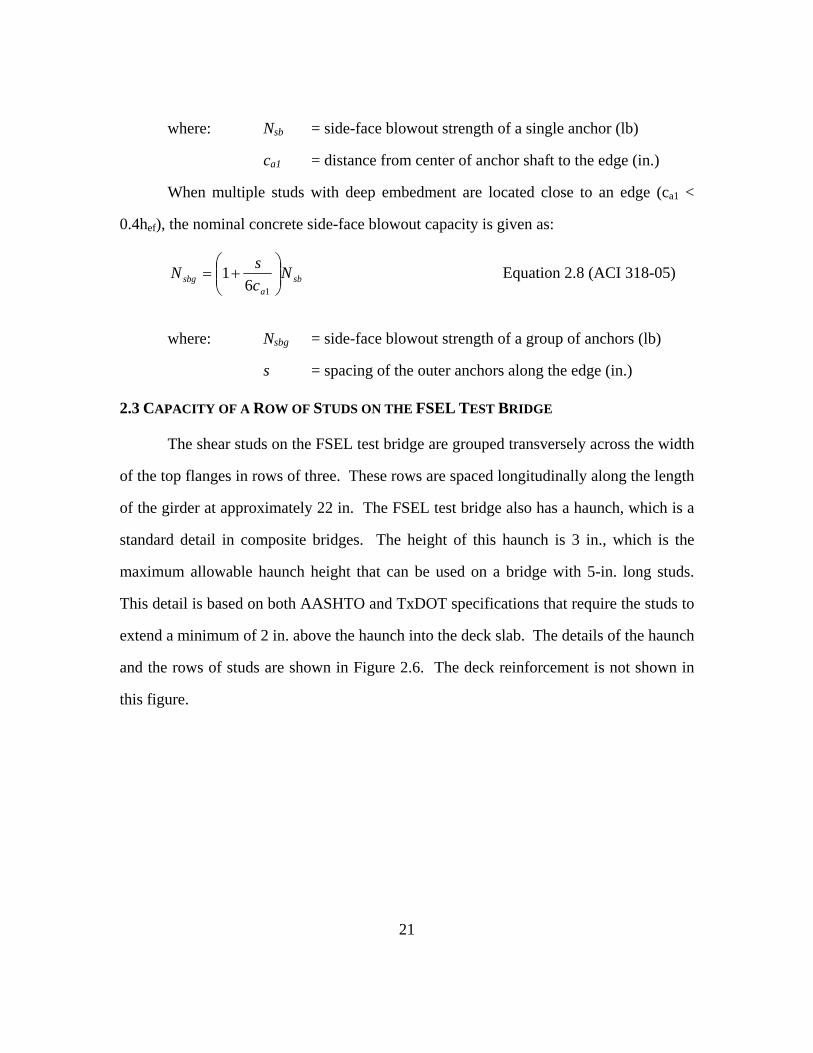
2.3 CAPACITY OF A ROW OF STUDS ON THE FSEL TEST BRIDGE
The shear studs on the FSEL test bridge are grouped transversely across the width
of the top flanges in rows of three. These rows are spaced longitudinally along the length
of the girder at approximately 22 in. The FSEL test bridge also has a haunch, which is a
standard detail in composite bridges. The height of this haunch is 3 in., which is the
maximum allowable haunch height that can be used on a bridge with 5-in. long studs.
This detail is based on both AASHTO and TxDOT specifications that require the studs to
extend a minimum of 2 in. above the haunch into the deck slab. The details of the haunch
and the rows of studs are shown in Figure 2.6. The deck reinforcement is not shown in
this figure.
22
5"
( = 9")
8"
3"
1.5" 1.5"2 Spa @ 4.5"
Figure 2.6: Shear stud detail for FSEL test bridge
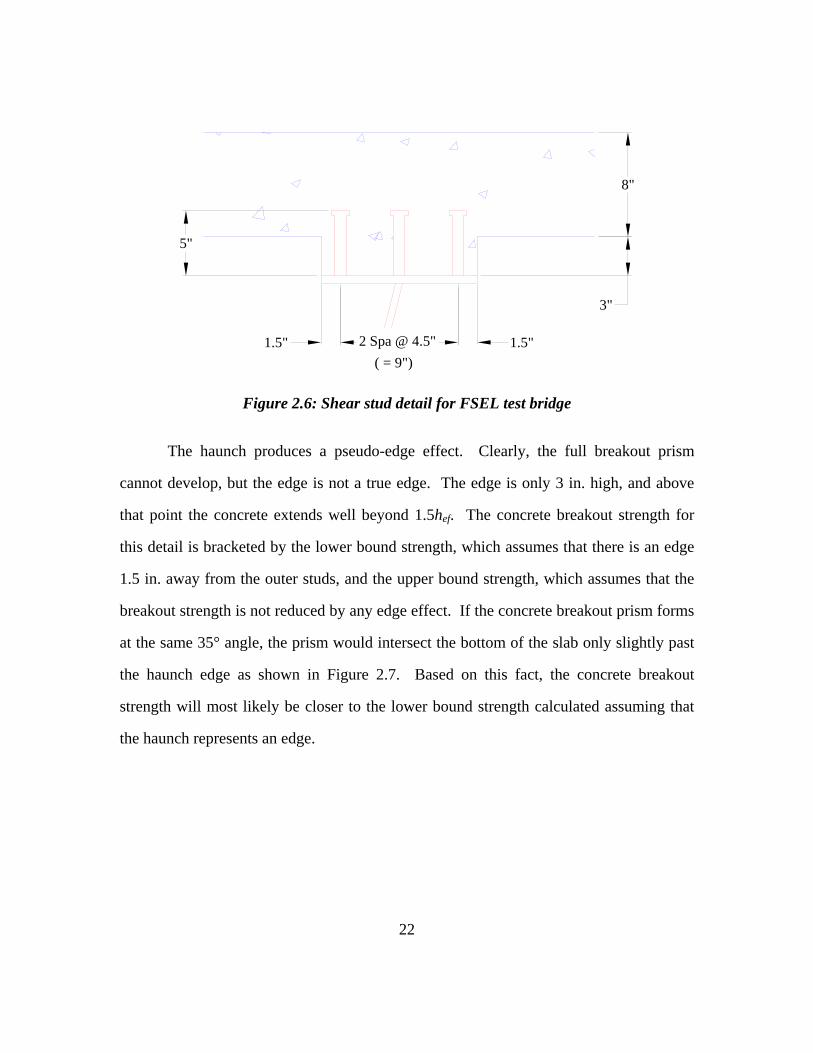
The haunch produces a pseudo-edge effect. Clearly, the full breakout prism
cannot develop, but the edge is not a true edge. The edge is only 3 in. high, and above
that point the concrete extends well beyond 1.5hef. The concrete breakout strength for
this detail is bracketed by the lower bound strength, which assumes that there is an edge
1.5 in. away from the outer studs, and the upper bound strength, which assumes that the
breakout strength is not reduced by any edge effect. If the concrete breakout prism forms
at the same 35° angle, the prism would intersect the bottom of the slab only slightly past
the haunch edge as shown in Figure 2.7. Based on this fact, the concrete breakout
strength will most likely be closer to the lower bound strength calculated assuming that
the haunch represents an edge.
23
Figure 2.7: Concrete breakout prism following 35° angle
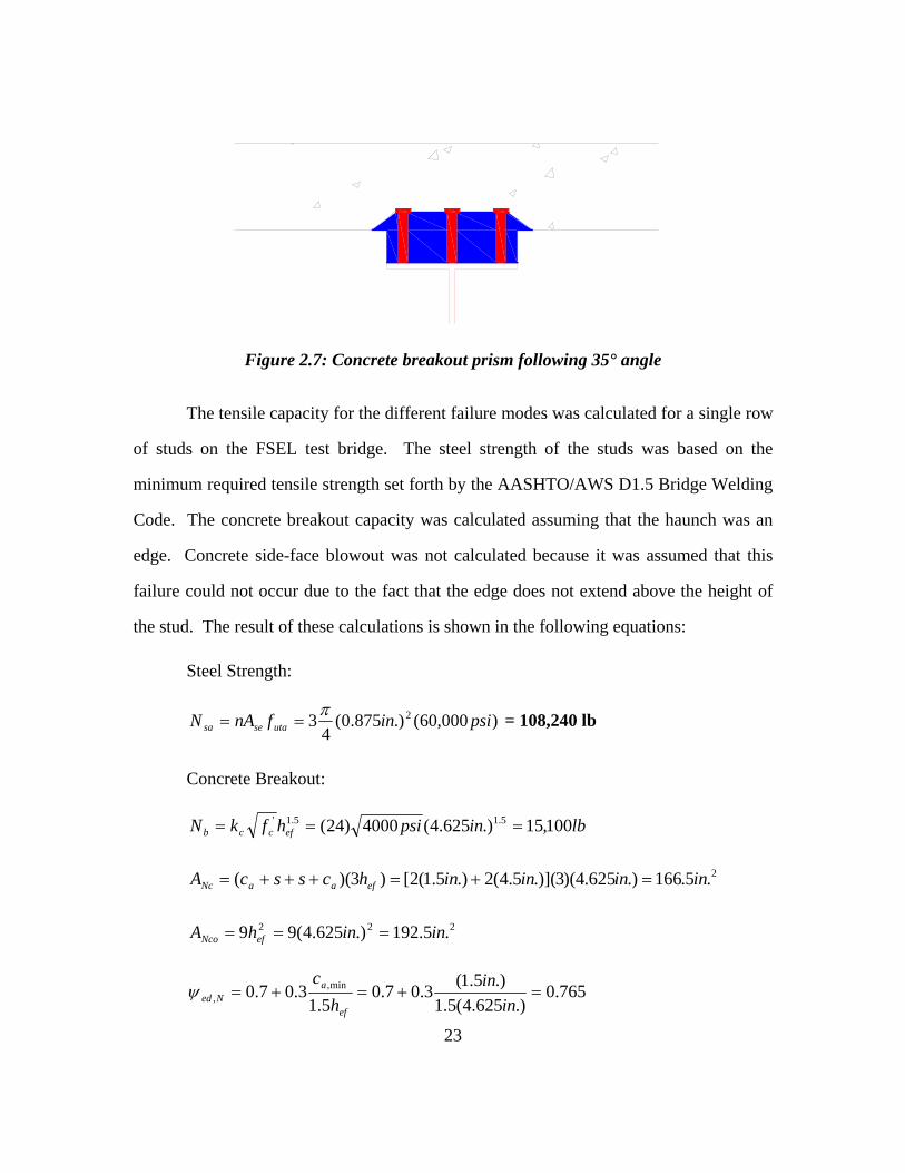
The tensile capacity for the different failure modes was calculated for a single row
of studs on the FSEL test bridge. The steel strength of the studs was based on the
minimum required tensile strength set forth by the AASHTO/AWS D1.5 Bridge Welding
Code. The concrete breakout capacity was calculated assuming that the haunch was an
edge. Concrete side-face blowout was not calculated because it was assumed that this
failure could not occur due to the fact that the edge does not extend above the height of
the stud. The result of these calculations is shown in the following equations:
Steel Strength:
)000,60(.)875.0(4
3 2 psiinfnAN utasesaπ
== = 108,240 lb
Concrete Breakout:
lbinpsihfkN efccb 100,15.)625.4(4000)24( 5.15.1' ===
2.5.166.)625.4)(3.)](5.4(2.)5.1(2[)3)(( ininininhcsscA efaaNc =+=+++=
222 .5.192.)625.4(99 ininhA efNco ===
765.0.)625.4(5.1
.)5.1(3.07.05.1
3.07.0 min,, =+=+=
inin
hc
ef
aNedψ
24
)100,15)(0.1)(765.0)(0.1().5.192().5.166(
2
2
,,, lbininN
AA
N bNcNedNecNco
Nccbg == ψψψ = 9,990 lb
Pullout (of 1 stud):
)000,4)(.)875.0(.)375.1((4
)8)(0.1(8 22', psiininfAN cbrgpcpn −==
πψ = 28,270 lb
These calculations show that concrete breakout is clearly the governing failure
mode. Even if it was assumed that the haunch had no effect, concrete breakout would
still be the governing failure mode. The estimated breakout capacity of a row of studs
(Ncbg) on the FSEL test bridge was rounded to 10 kips. The modification factor for
eccentric loading (ψec,N) was taken as 1.0 because the load is not applied eccentrically,
and the modification factor for cracking (ψc,N) was taken as 1.0 because it was assumed
that the deck slab will be cracked after the fracture.
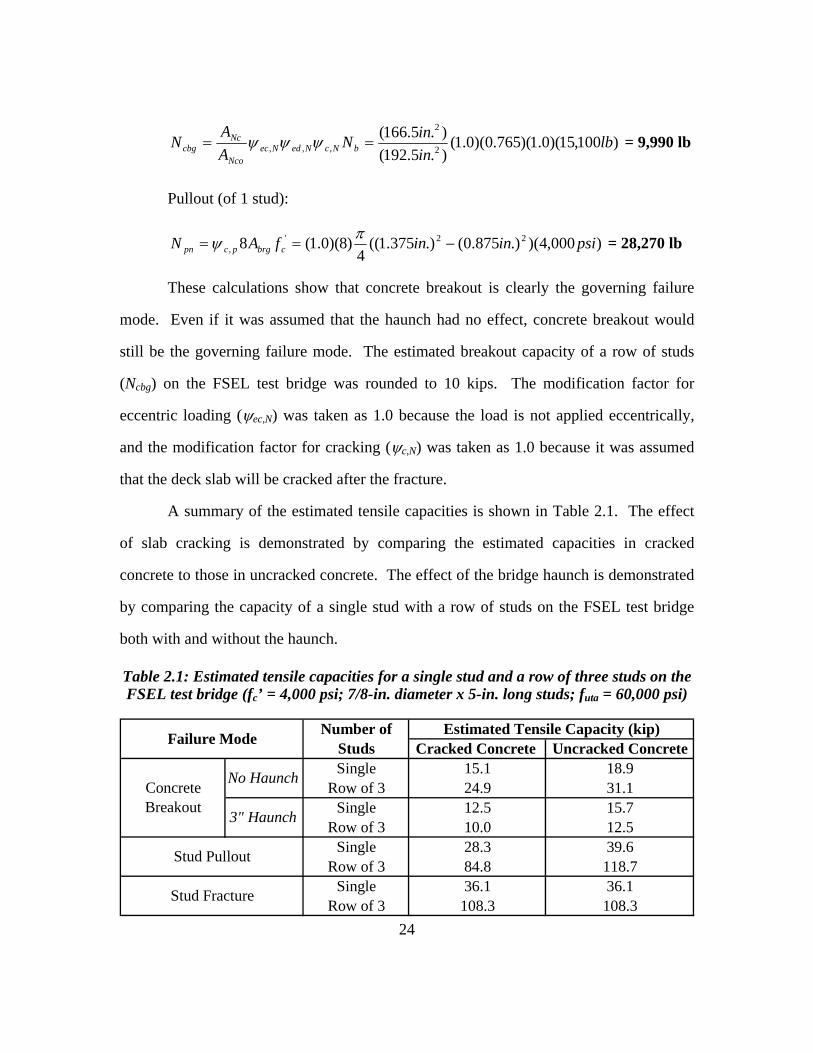
A summary of the estimated tensile capacities is shown in Table 2.1. The effect
of slab cracking is demonstrated by comparing the estimated capacities in cracked
concrete to those in uncracked concrete. The effect of the bridge haunch is demonstrated
by comparing the capacity of a single stud with a row of studs on the FSEL test bridge
both with and without the haunch.
Table 2.1: Estimated tensile capacities for a single stud and a row of three studs on the FSEL test bridge (fc’ = 4,000 psi; 7/8-in. diameter x 5-in. long studs; futa = 60,000 psi)
Cracked Concrete Uncracked Concrete15.1 18.924.9 31.112.5 15.710.0 12.528.3 39.684.8 118.736.1 36.1
108.3 108.3Row of 3Single
Stud Pullout
Failure Mode Number of Studs
Estimated Tensile Capacity (kip)
Row of 3Single
Row of 3Single
Row of 3Single
Stud Fracture
Concrete Breakout
No Haunch
3" Haunch
25
If a single row of studs can resist 10 kips, then 56 rows of studs are required to
resist the 554-kip force from the fractured girder. The stud rows are spaced at 22 in.;
therefore, 103 ft, or 87% of the span length, is required to resist the 554-kip force.
Spreading the force among 56 rows assumes that the studs can behave in a ductile
manner and redistribute the force along the length of the girder. However, a concrete
breakout failure is governed by brittle failure of the concrete. This aspect of the response
may prevent the 554-kip force from being distributed among such a large percentage of
the span length.
2.4 SUMMARY
The calculations in this chapter have shown that the governing failure mode for a
row of shear studs on the FSEL test bridge is a concrete breakout failure. The concrete
breakout capacity of a row of three studs is greatly reduced when the studs are located
close to an edge. The haunch used in bridge construction produces a pseudo-edge very
close to the outer studs in the row. Therefore, it is assumed that the capacity of a row of
studs will be reduced, but the magnitude of the reduction can only be estimated using the
ACI 318 equations. Furthermore, while the strength of the studs appears to be adequate,
the studs may not be able to redistribute forces along the span due to the brittle nature of
a concrete breakout failure.
The remainder of this thesis will discuss the laboratory tests that were performed
to determine the effect that the bridge haunch has on both the capacity and the behavior
of the shear studs loaded in tension. The laboratory tests will also include the effect of
slab cracking due to a moment being applied to the deck slab in addition to the tensile
force acting on the studs.
26
CHAPTER 3
Testing Program
3.1 INTRODUCTION
The bridge haunch creates a great deal of uncertainty in the calculation of the
tensile capacity of the shear studs. The haunch is assumed to have a detrimental effect
because the full volume of the concrete breakout prism cannot be developed. The goal of
this testing program is to quantify the effect that the haunch has on the tensile capacity of
the shear studs.
Pullout tests were performed on 12 reinforced bridge deck sections. Half of these
deck sections were constructed with a haunch, while the other half have no haunch. The
number of studs was varied for both the specimens with and without a haunch. For the
specimens with a haunch, increasing the number of studs decreases the spacing between
the studs and the edge of the haunch. Theoretically, as this edge spacing decreases, the
capacity will decrease. For the specimens without a haunch, increasing the number of
studs should increase the capacity because the volume of concrete in the breakout failure
prism is increased.
When one of the bridge girders fractures, that girder will drop down, loading the
studs in tension and also loading the deck slab in bending. This situation is duplicated in
the laboratory tests. The studs will be loaded in tension, but the tension force used to
load the studs also creates a bending moment in the slab. However, it is important to
realize that test setup will not exactly replicate the situation in the bridge. Prior to a
fracture, the deck slab of the bridge experiences compressive stresses due to the
27
longitudinal bending of the composite section. The deck sections tested in the laboratory
do not have any initial stresses in the slab due to longitudinal bending.
3.2 TEST SPECIMENS
3.2.1 Specimen Details
Six unique reinforced composite deck sections were tested. A duplicate of each
specimen was tested for a total of 12 tests. Half of the specimens were constructed with a
3-in. haunch while the other half was constructed with no haunch. When selecting the
dimensions and details to be used in the specimens, every effort was taken to replicate the
details built into the full scale test bridge at FSEL, which uses typical TxDOT bridge
deck details. Refer to Appendix B for the TxDOT details and the deck slab details of the
test bridge at FSEL, from which all of the specimen details were based. Refer to
Appendix C for the detailed drawings of all six unique specimens.
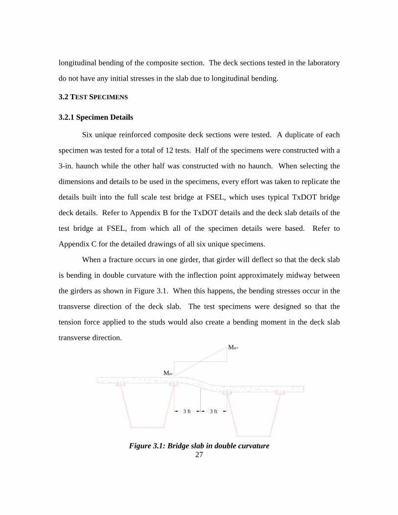
When a fracture occurs in one girder, that girder will deflect so that the deck slab
is bending in double curvature with the inflection point approximately midway between
the girders as shown in Figure 3.1. When this happens, the bending stresses occur in the
transverse direction of the deck slab. The test specimens were designed so that the
tension force applied to the studs would also create a bending moment in the deck slab
transverse direction. Mn+
Mn-
3 ft 3 ft
Figure 3.1: Bridge slab in double curvature
28
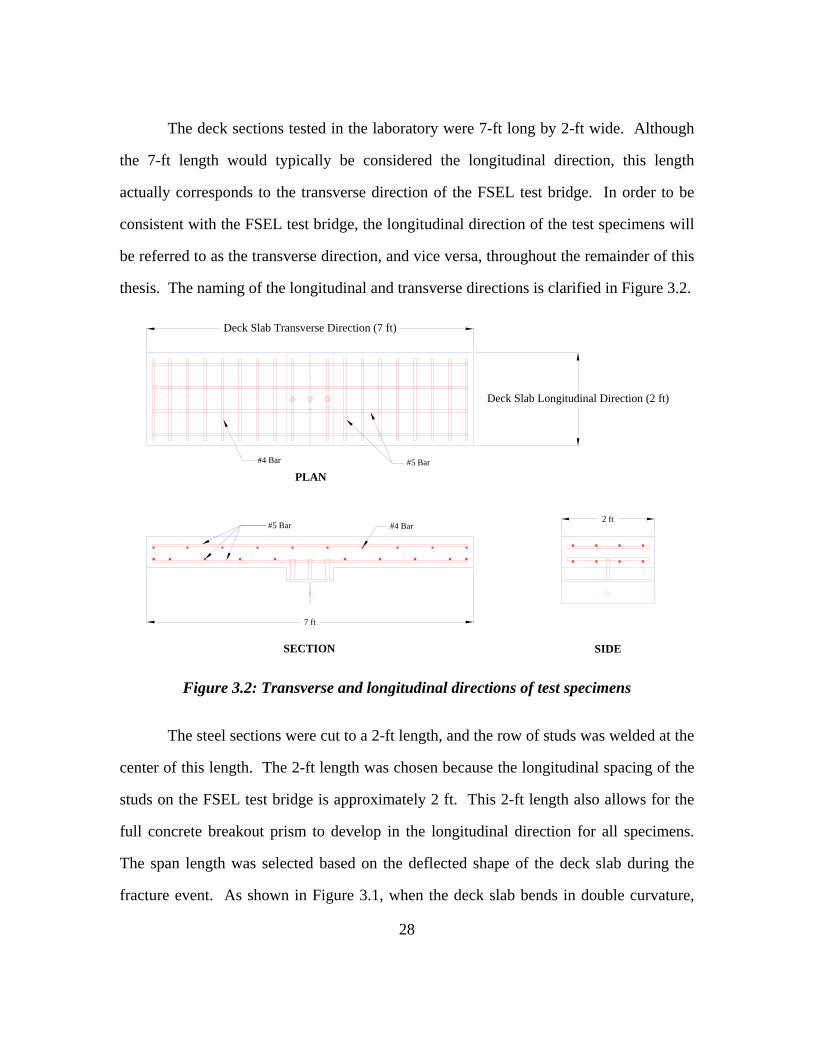
The deck sections tested in the laboratory were 7-ft long by 2-ft wide. Although
the 7-ft length would typically be considered the longitudinal direction, this length
actually corresponds to the transverse direction of the FSEL test bridge. In order to be
consistent with the FSEL test bridge, the longitudinal direction of the test specimens will
be referred to as the transverse direction, and vice versa, throughout the remainder of this
thesis. The naming of the longitudinal and transverse directions is clarified in Figure 3.2.
#5 Bar#4 Bar
7 ft
2 ft
PLAN
SECTION SIDE
Deck Slab Transverse Direction (7 ft)
Deck Slab Longitudinal Direction (2 ft)
#4 Bar#5 Bar
Figure 3.2: Transverse and longitudinal directions of test specimens
The steel sections were cut to a 2-ft length, and the row of studs was welded at the
center of this length. The 2-ft length was chosen because the longitudinal spacing of the
studs on the FSEL test bridge is approximately 2 ft. This 2-ft length also allows for the
full concrete breakout prism to develop in the longitudinal direction for all specimens.
The span length was selected based on the deflected shape of the deck slab during the
fracture event. As shown in Figure 3.1, when the deck slab bends in double curvature,
29
the maximum moment in the deck slab occurs at the shear stud connection, and the
distance between the inflection point and the studs is approximately 3 ft. The test
specimens were tested as simply supported slabs with a tension force loading the studs at
the mid-span. This arrangement allowed the maximum moment to occur at the location
of the stud connection. The span length of approximately 6 ft was chosen because it
corresponds to 3 ft from the point of zero moment to maximum moment as is the case
when the deck slab bends in double curvature. The 7-ft overall length was chosen so that
an adequate bearing length was available at each end. The 6-ft span is also long enough
to assure that an adequate moment is present in the slab, but short enough that a tension
failure of the studs will occur before a bending failure of the slab.
The slab thickness was chosen to be 8 in. because it matches the thickness of the
deck slab on the FSEL test bridge. The size and spacing of the slab reinforcement was
based on the typical TxDOT deck slab details, which are also used in the FSEL test
bridge. The reinforcement consisted of a top and bottom mat of reinforcing steel with
bars running in both the transverse and longitudinal directions as also shown by Figure
3.2. The top and bottom transverse bars and the bottom longitudinal bars are all #5 bars.
The top longitudinal bars are all #4 bars. The transverse bars are spaced at 6 in., and the
longitudinal bars are spaced at 9 in. The clear cover was 1.25 in. and 2 in. to the bottom
and top reinforcing mat, respectively.
The steel section used for each specimen is a WT6x39.5. This section was
selected because the top flange width, top flange thickness, and web thickness of the
WT6x39.5 very closely matches the top flange width, top flange thickness, and web
thickness of the box girders on the FSEL test bridge.
The studs used in the test specimens had a diameter of 7/8 in. and a length of 5 in.
These stud dimensions were selected to match the studs used in the FSEL test bridge.
30
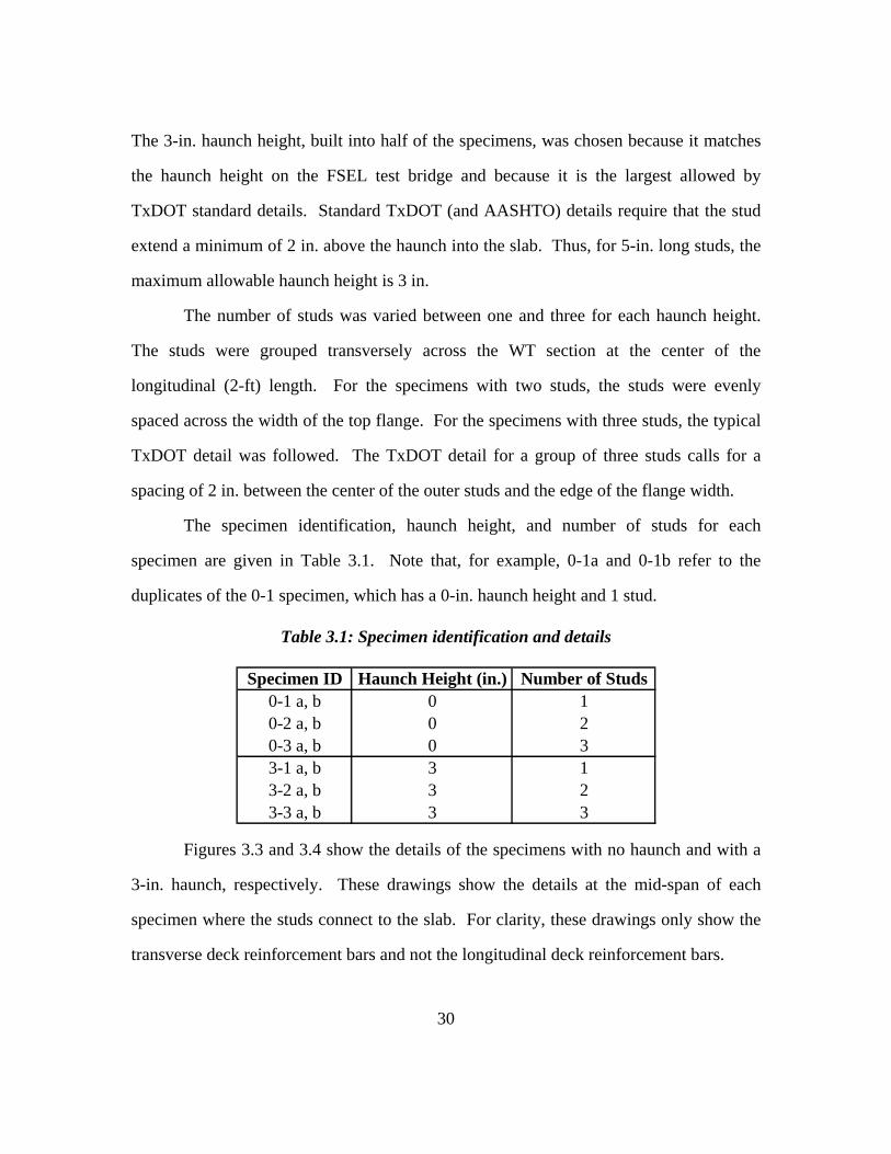
The 3-in. haunch height, built into half of the specimens, was chosen because it matches
the haunch height on the FSEL test bridge and because it is the largest allowed by
TxDOT standard details. Standard TxDOT (and AASHTO) details require that the stud
extend a minimum of 2 in. above the haunch into the slab. Thus, for 5-in. long studs, the
maximum allowable haunch height is 3 in.
The number of studs was varied between one and three for each haunch height.
The studs were grouped transversely across the WT section at the center of the
longitudinal (2-ft) length. For the specimens with two studs, the studs were evenly
spaced across the width of the top flange. For the specimens with three studs, the typical
TxDOT detail was followed. The TxDOT detail for a group of three studs calls for a
spacing of 2 in. between the center of the outer studs and the edge of the flange width.
The specimen identification, haunch height, and number of studs for each
specimen are given in Table 3.1. Note that, for example, 0-1a and 0-1b refer to the
duplicates of the 0-1 specimen, which has a 0-in. haunch height and 1 stud.
Table 3.1: Specimen identification and details
Specimen ID Haunch Height (in.) Number of Studs0-1 a, b 0 10-2 a, b 0 20-3 a, b 0 33-1 a, b 3 13-2 a, b 3 23-3 a, b 3 3
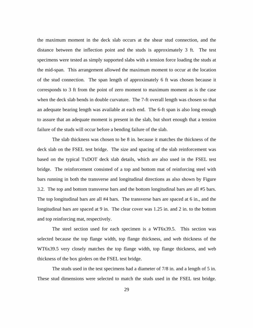
Figures 3.3 and 3.4 show the details of the specimens with no haunch and with a
3-in. haunch, respectively. These drawings show the details at the mid-span of each
specimen where the studs connect to the slab. For clarity, these drawings only show the
transverse deck reinforcement bars and not the longitudinal deck reinforcement bars.
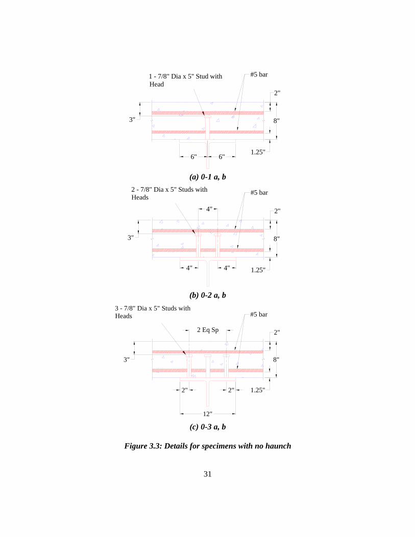
31
1 - 7/8" Dia x 5" Stud with Head
8"3"
6" 6"1.25"
2"
#5 bar
(a) 0-1 a, b
2 - 7/8" Dia x 5" Studs with Heads
8"
4"
4" 4"
3"
1.25"
2"
#5 bar
(b) 0-2 a, b
3 - 7/8" Dia x 5" Studs with Heads
8"
2" 2"
3"
2 Eq Sp
12"
1.25"
2"
#5 bar
(c) 0-3 a, b
Figure 3.3: Details for specimens with no haunch
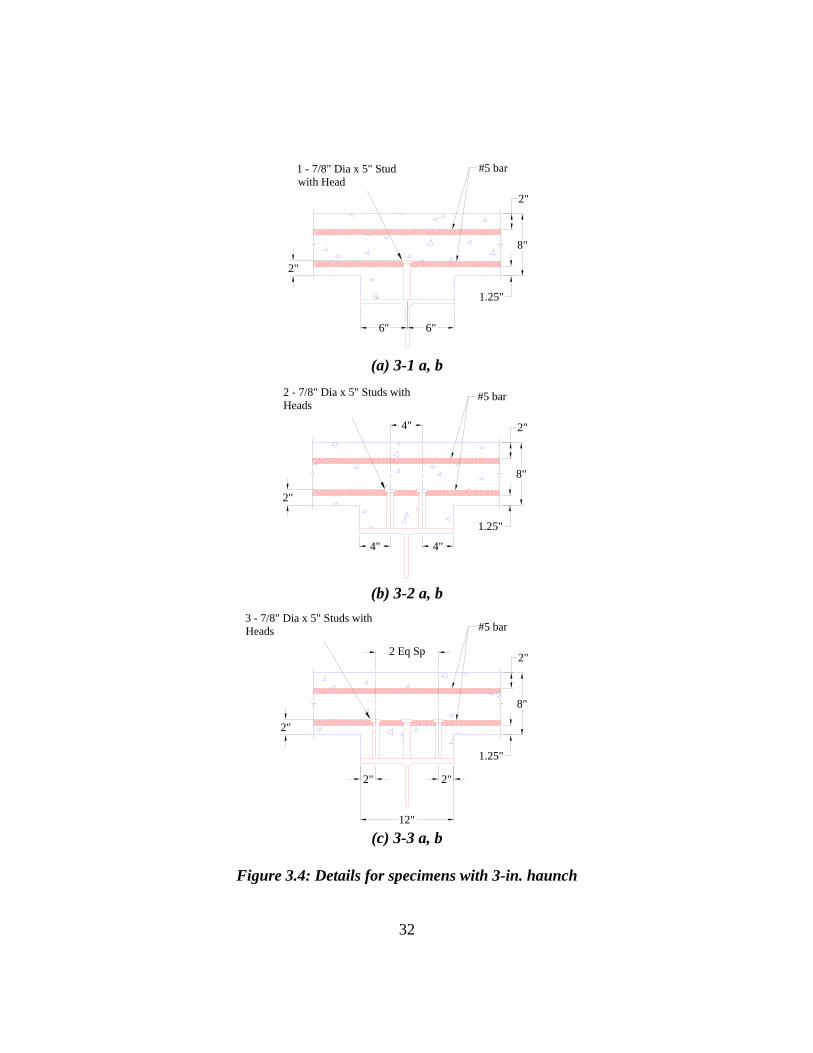
32
1 - 7/8" Dia x 5" Stud with Head
8"
2"
6" 6"
1.25"
2"
#5 bar
(a) 3-1 a, b
2 - 7/8" Dia x 5" Studs with Heads
8"
2"
4"
4" 4"
1.25"
2"
#5 bar
(b) 3-2 a, b
3 - 7/8" Dia x 5" Studs with Heads
8"
2"
2 Eq Sp
2" 2"
12"
1.25"
2"
#5 bar
(c) 3-3 a, b
Figure 3.4: Details for specimens with 3-in. haunch
33
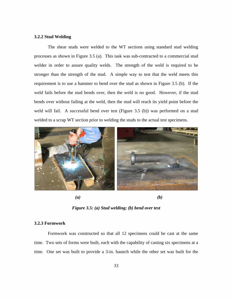
3.2.2 Stud Welding
The shear studs were welded to the WT sections using standard stud welding
processes as shown in Figure 3.5 (a). This task was sub-contracted to a commercial stud
welder in order to assure quality welds. The strength of the weld is required to be
stronger than the strength of the stud. A simple way to test that the weld meets this
requirement is to use a hammer to bend over the stud as shown in Figure 3.5 (b). If the
weld fails before the stud bends over, then the weld is no good. However, if the stud
bends over without failing at the weld, then the stud will reach its yield point before the
weld will fail. A successful bend over test (Figure 3.5 (b)) was performed on a stud
welded to a scrap WT section prior to welding the studs to the actual test specimens.
(a) (b)
Figure 3.5: (a) Stud welding; (b) bend over test
3.2.3 Formwork
Formwork was constructed so that all 12 specimens could be cast at the same
time. Two sets of forms were built, each with the capability of casting six specimens at a
time. One set was built to provide a 3-in. haunch while the other set was built for the
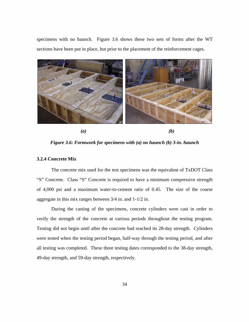
34
specimens with no haunch. Figure 3.6 shows these two sets of forms after the WT
sections have been put in place, but prior to the placement of the reinforcement cages.
(a) (b)
Figure 3.6: Formwork for specimens with (a) no haunch (b) 3-in. haunch
3.2.4 Concrete Mix
The concrete mix used for the test specimens was the equivalent of TxDOT Class
“S” Concrete. Class “S” Concrete is required to have a minimum compressive strength
of 4,000 psi and a maximum water-to-cement ratio of 0.45. The size of the coarse
aggregate in this mix ranges between 3/4 in. and 1-1/2 in.
During the casting of the specimens, concrete cylinders were cast in order to
verify the strength of the concrete at various periods throughout the testing program.
Testing did not begin until after the concrete had reached its 28-day strength. Cylinders
were tested when the testing period began, half-way through the testing period, and after
all testing was completed. These three testing dates corresponded to the 38-day strength,
49-day strength, and 59-day strength, respectively.
35
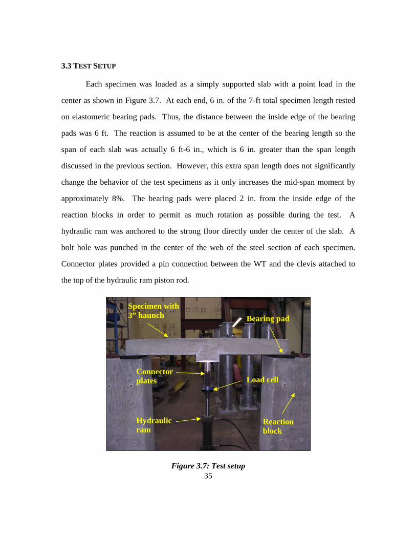
3.3 TEST SETUP
Each specimen was loaded as a simply supported slab with a point load in the
center as shown in Figure 3.7. At each end, 6 in. of the 7-ft total specimen length rested
on elastomeric bearing pads. Thus, the distance between the inside edge of the bearing
pads was 6 ft. The reaction is assumed to be at the center of the bearing length so the
span of each slab was actually 6 ft-6 in., which is 6 in. greater than the span length
discussed in the previous section. However, this extra span length does not significantly
change the behavior of the test specimens as it only increases the mid-span moment by
approximately 8%. The bearing pads were placed 2 in. from the inside edge of the
reaction blocks in order to permit as much rotation as possible during the test. A
hydraulic ram was anchored to the strong floor directly under the center of the slab. A
bolt hole was punched in the center of the web of the steel section of each specimen.
Connector plates provided a pin connection between the WT and the clevis attached to
the top of the hydraulic ram piston rod.
Figure 3.7: Test setup
Hydraulic ram
Load cell
Reaction block
Specimen with 3” haunch Bearing pad
Connector plates
36
3.4 INSTRUMENTATION
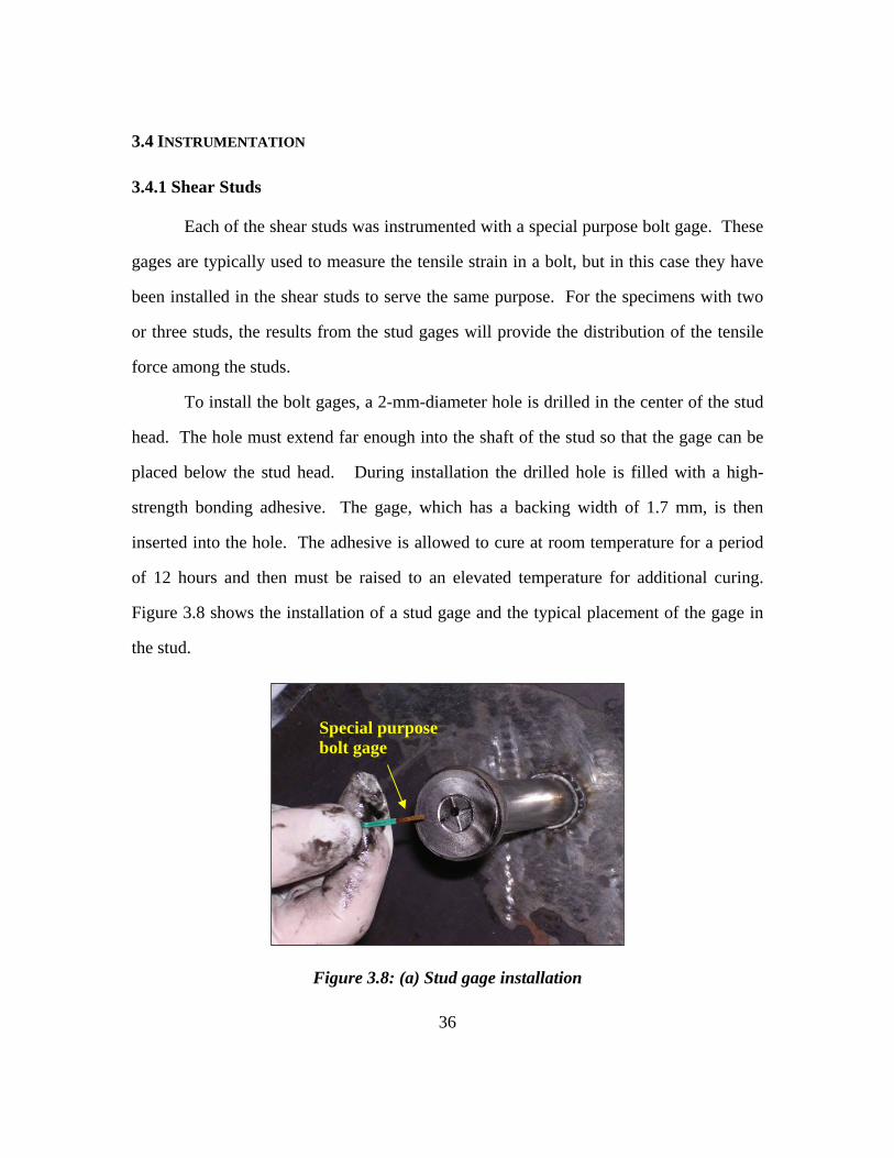
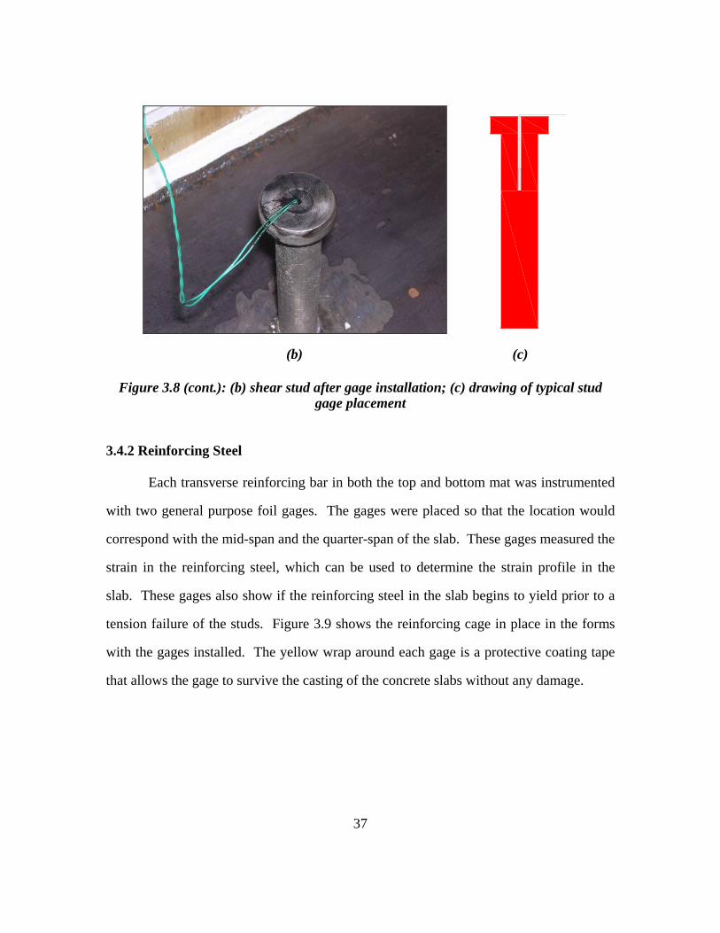
3.4.1 Shear Studs
Each of the shear studs was instrumented with a special purpose bolt gage. These
gages are typically used to measure the tensile strain in a bolt, but in this case they have
been installed in the shear studs to serve the same purpose. For the specimens with two
or three studs, the results from the stud gages will provide the distribution of the tensile
force among the studs.
To install the bolt gages, a 2-mm-diameter hole is drilled in the center of the stud
head. The hole must extend far enough into the shaft of the stud so that the gage can be
placed below the stud head. During installation the drilled hole is filled with a high-
strength bonding adhesive. The gage, which has a backing width of 1.7 mm, is then
inserted into the hole. The adhesive is allowed to cure at room temperature for a period
of 12 hours and then must be raised to an elevated temperature for additional curing.
Figure 3.8 shows the installation of a stud gage and the typical placement of the gage in
the stud.
Figure 3.8: (a) Stud gage installation
Special purpose bolt gage
37
(b) (c)
Figure 3.8 (cont.): (b) shear stud after gage installation; (c) drawing of typical stud gage placement
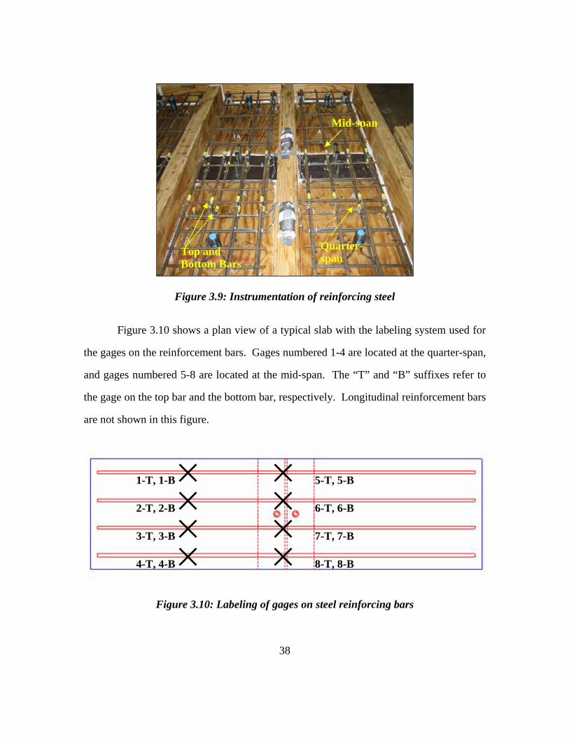
3.4.2 Reinforcing Steel
Each transverse reinforcing bar in both the top and bottom mat was instrumented
with two general purpose foil gages. The gages were placed so that the location would
correspond with the mid-span and the quarter-span of the slab. These gages measured the
strain in the reinforcing steel, which can be used to determine the strain profile in the
slab. These gages also show if the reinforcing steel in the slab begins to yield prior to a
tension failure of the studs. Figure 3.9 shows the reinforcing cage in place in the forms
with the gages installed. The yellow wrap around each gage is a protective coating tape
that allows the gage to survive the casting of the concrete slabs without any damage.
38
Figure 3.9: Instrumentation of reinforcing steel
Figure 3.10 shows a plan view of a typical slab with the labeling system used for
the gages on the reinforcement bars. Gages numbered 1-4 are located at the quarter-span,
and gages numbered 5-8 are located at the mid-span. The “T” and “B” suffixes refer to
the gage on the top bar and the bottom bar, respectively. Longitudinal reinforcement bars
are not shown in this figure.
Figure 3.10: Labeling of gages on steel reinforcing bars
Top and Bottom Bars
Quarter-span
Mid-span
1-T, 1-B
2-T, 2-B
8-T, 8-B
3-T, 3-B
4-T, 4-B
7-T, 7-B
6-T, 6-B
5-T, 5-B
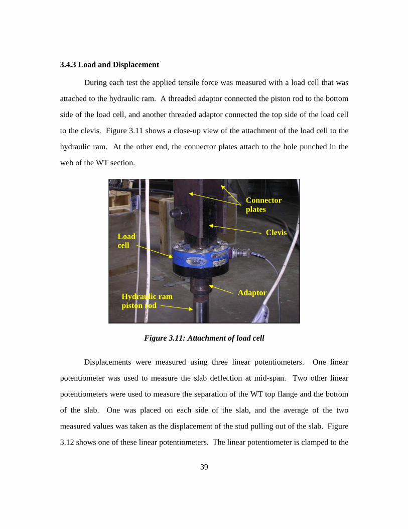
39
3.4.3 Load and Displacement
During each test the applied tensile force was measured with a load cell that was
attached to the hydraulic ram. A threaded adaptor connected the piston rod to the bottom
side of the load cell, and another threaded adaptor connected the top side of the load cell
to the clevis. Figure 3.11 shows a close-up view of the attachment of the load cell to the
hydraulic ram. At the other end, the connector plates attach to the hole punched in the
web of the WT section.
Figure 3.11: Attachment of load cell
Displacements were measured using three linear potentiometers. One linear
potentiometer was used to measure the slab deflection at mid-span. Two other linear
potentiometers were used to measure the separation of the WT top flange and the bottom
of the slab. One was placed on each side of the slab, and the average of the two
measured values was taken as the displacement of the stud pulling out of the slab. Figure
3.12 shows one of these linear potentiometers. The linear potentiometer is clamped to the
Hydraulic ram piston rod
Load cell
Connector plates
Adaptor
Clevis
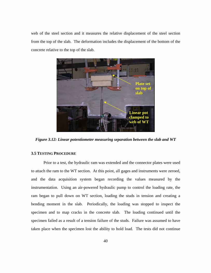
40
web of the steel section and it measures the relative displacement of the steel section
from the top of the slab. The deformation includes the displacement of the bottom of the
concrete relative to the top of the slab.
Figure 3.12: Linear potentiometer measuring separation between the slab and WT
3.5 TESTING PROCEDURE
Prior to a test, the hydraulic ram was extended and the connector plates were used
to attach the ram to the WT section. At this point, all gages and instruments were zeroed,
and the data acquisition system began recording the values measured by the
instrumentation. Using an air-powered hydraulic pump to control the loading rate, the
ram began to pull down on WT section, loading the studs in tension and creating a
bending moment in the slab. Periodically, the loading was stopped to inspect the
specimen and to map cracks in the concrete slab. The loading continued until the
specimen failed as a result of a tension failure of the studs. Failure was assumed to have
taken place when the specimen lost the ability to hold load. The tests did not continue
Linear pot clamped to web of WT
Plate set on top of slab
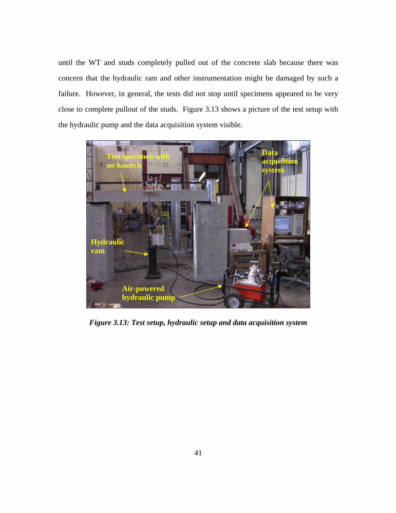
41
until the WT and studs completely pulled out of the concrete slab because there was
concern that the hydraulic ram and other instrumentation might be damaged by such a
failure. However, in general, the tests did not stop until specimens appeared to be very
close to complete pullout of the studs. Figure 3.13 shows a picture of the test setup with
the hydraulic pump and the data acquisition system visible.
Figure 3.13: Test setup, hydraulic setup and data acquisition system
Air-powered hydraulic pump
Data acquisition system
Hydraulic ram
Test specimen with no haunch
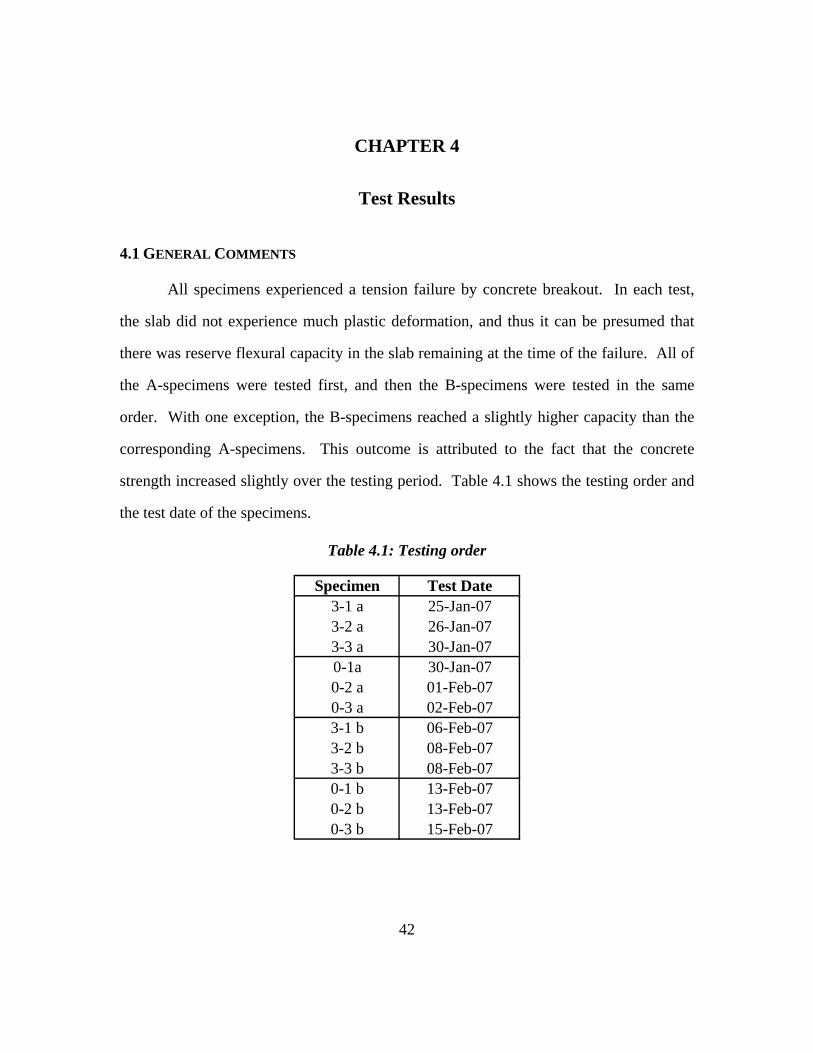
42
CHAPTER 4
Test Results
4.1 GENERAL COMMENTS
All specimens experienced a tension failure by concrete breakout. In each test,
the slab did not experience much plastic deformation, and thus it can be presumed that
there was reserve flexural capacity in the slab remaining at the time of the failure. All of
the A-specimens were tested first, and then the B-specimens were tested in the same
order. With one exception, the B-specimens reached a slightly higher capacity than the
corresponding A-specimens. This outcome is attributed to the fact that the concrete
strength increased slightly over the testing period. Table 4.1 shows the testing order and
the test date of the specimens.
Table 4.1: Testing order
Specimen Test Date3-1 a 25-Jan-073-2 a 26-Jan-073-3 a 30-Jan-070-1a 30-Jan-070-2 a 01-Feb-070-3 a 02-Feb-073-1 b 06-Feb-073-2 b 08-Feb-073-3 b 08-Feb-070-1 b 13-Feb-070-2 b 13-Feb-070-3 b 15-Feb-07
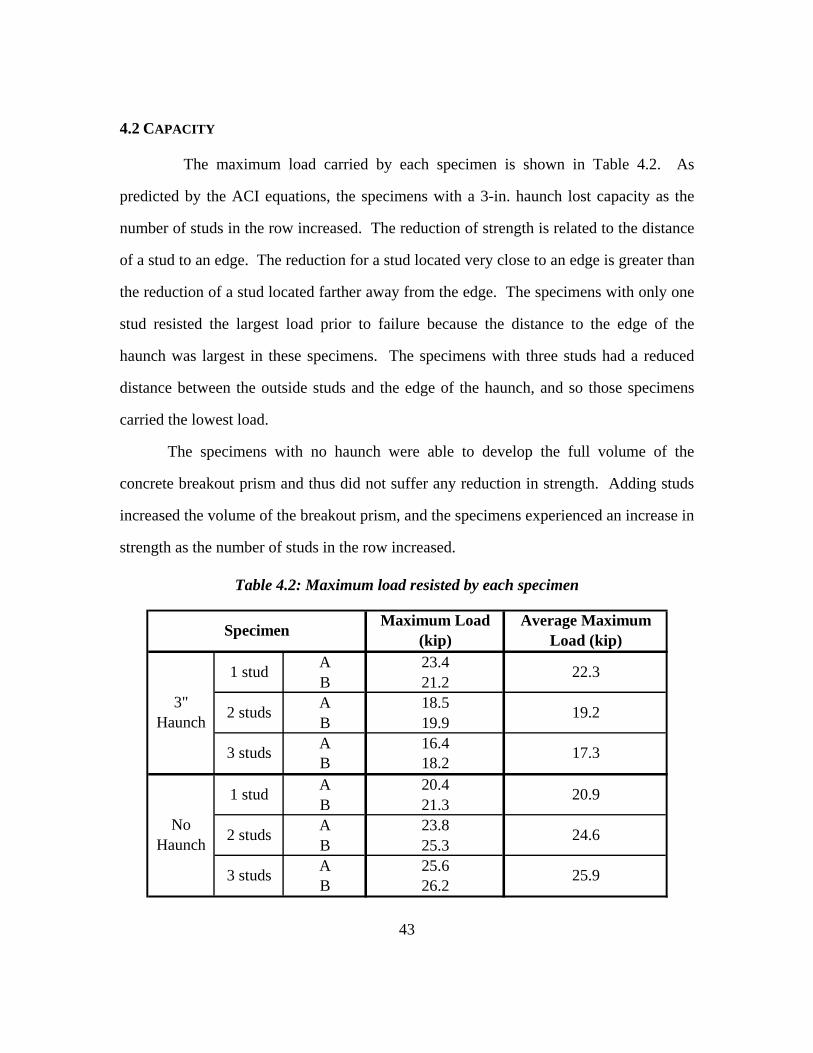
43
4.2 CAPACITY
The maximum load carried by each specimen is shown in Table 4.2. As
predicted by the ACI equations, the specimens with a 3-in. haunch lost capacity as the
number of studs in the row increased. The reduction of strength is related to the distance
of a stud to an edge. The reduction for a stud located very close to an edge is greater than
the reduction of a stud located farther away from the edge. The specimens with only one
stud resisted the largest load prior to failure because the distance to the edge of the
haunch was largest in these specimens. The specimens with three studs had a reduced
distance between the outside studs and the edge of the haunch, and so those specimens
carried the lowest load.
The specimens with no haunch were able to develop the full volume of the
concrete breakout prism and thus did not suffer any reduction in strength. Adding studs
increased the volume of the breakout prism, and the specimens experienced an increase in
strength as the number of studs in the row increased.
Table 4.2: Maximum load resisted by each specimen
A 23.4B 21.2A 18.5B 19.9A 16.4B 18.2A 20.4B 21.3A 23.8B 25.3A 25.6B 26.2
Maximum Load (kip)
Average Maximum Load (kip)
3" Haunch
No Haunch
Specimen
2 studs 24.6
3 studs 25.9
3 studs 17.3
1 stud 20.9
1 stud 22.3
2 studs 19.2
44
The results in Table 4.2 show that the presence of a haunch can significantly
reduce the tensile capacity of a group of studs. For the specimens with only one stud, the
breakout capacity with a haunch and without a haunch is very close. In this case, the
specimens with a haunch actually reached slightly higher average maximum load than the
specimens without a haunch. However, the strengths of the two-stud and three-stud
specimens without a haunch were considerably higher than the two-stud and three-stud
specimens with a haunch.
The 3-in. haunch specimens with two and three studs show a large drop in the
breakout capacity when compared to the specimens with a haunch and only one stud. The
average capacity dropped 14% for the specimens with two studs and 23% for the
specimens with three studs. Conversely, the specimens without a haunch showed an
increase in strength when the number of studs was increased. However, the increase in
tensile strength is small, less than 25% for the three stud test versus the single stud test.
4.3 BEHAVIOR AT FAILURE
4.3.1 Specimens with a Haunch
Each specimen with a 3-in. haunch failed in a very sudden, brittle manner and
exhibited very little ductility. These specimens reached a maximum load, failed
suddenly, and immediately lost all ability to carry load. Figure 4.1 shows a plot of the
applied load versus the stud pullout deflection for a specimen with one stud. The plot
shows that the specimen reaches a maximum load and then fails very suddenly with the
next data point down near 0 kip. This plot is typical of all of the specimens with a 3-in.
haunch.
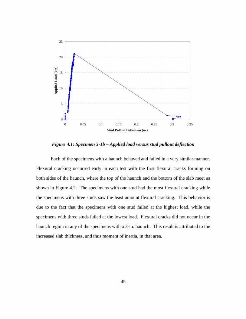
45
0
5
10
15
20
25
0 0.05 0.1 0.15 0.2 0.25 0.3 0.35
Stud Pullout Deflection (in.)
App
lied
Loa
d (k
ip)
Figure 4.1: Specimen 3-1b – Applied load versus stud pullout deflection
Each of the specimens with a haunch behaved and failed in a very similar manner.
Flexural cracking occurred early in each test with the first flexural cracks forming on
both sides of the haunch, where the top of the haunch and the bottom of the slab meet as
shown in Figure 4.2. The specimens with one stud had the most flexural cracking while
the specimens with three studs saw the least amount flexural cracking. This behavior is
due to the fact that the specimens with one stud failed at the highest load, while the
specimens with three studs failed at the lowest load. Flexural cracks did not occur in the
haunch region in any of the specimens with a 3-in. haunch. This result is attributed to the
increased slab thickness, and thus moment of inertia, in that area.
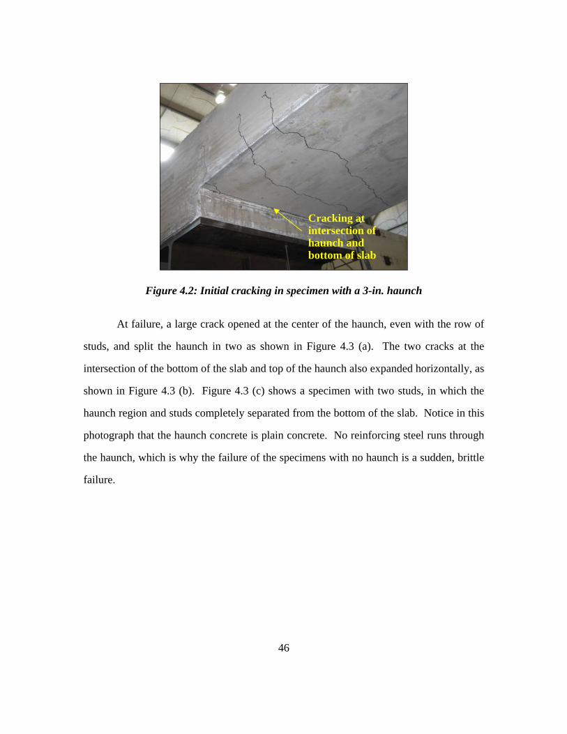
46
Figure 4.2: Initial cracking in specimen with a 3-in. haunch
At failure, a large crack opened at the center of the haunch, even with the row of
studs, and split the haunch in two as shown in Figure 4.3 (a). The two cracks at the
intersection of the bottom of the slab and top of the haunch also expanded horizontally, as
shown in Figure 4.3 (b). Figure 4.3 (c) shows a specimen with two studs, in which the
haunch region and studs completely separated from the bottom of the slab. Notice in this
photograph that the haunch concrete is plain concrete. No reinforcing steel runs through
the haunch, which is why the failure of the specimens with no haunch is a sudden, brittle
failure.
Cracking at intersection of haunch and bottom of slab
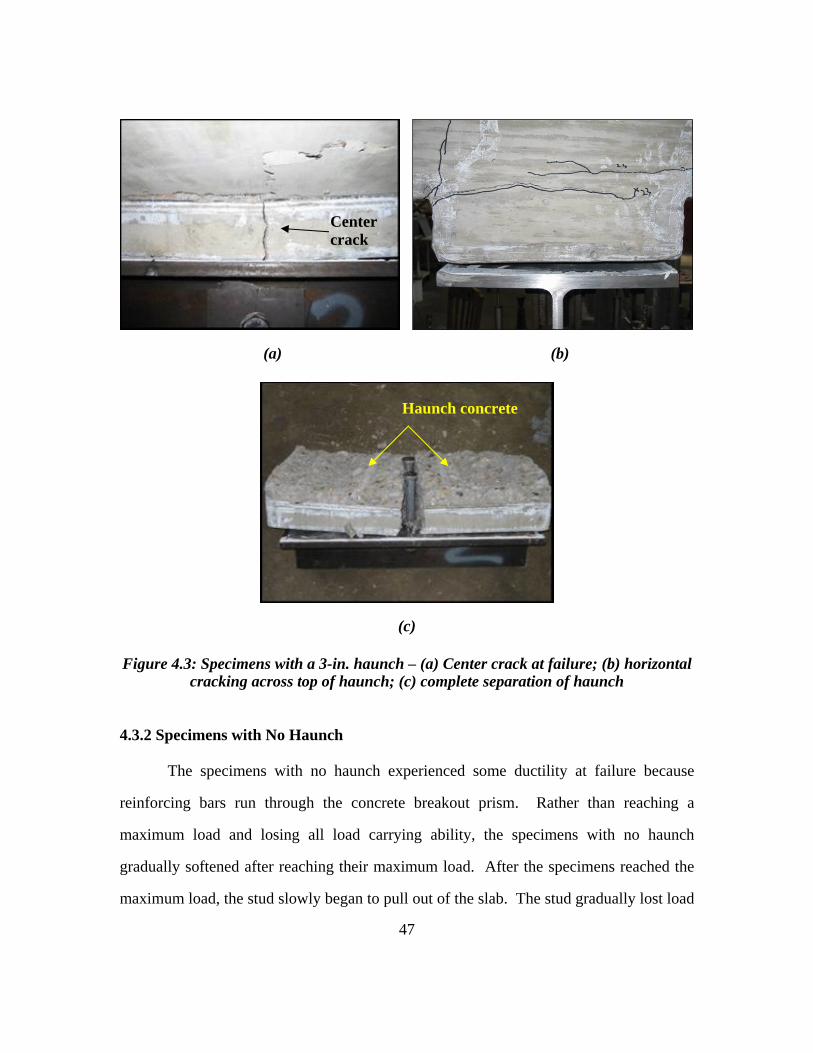
47
(a) (b)
(c)
Figure 4.3: Specimens with a 3-in. haunch – (a) Center crack at failure; (b) horizontal cracking across top of haunch; (c) complete separation of haunch
4.3.2 Specimens with No Haunch
The specimens with no haunch experienced some ductility at failure because
reinforcing bars run through the concrete breakout prism. Rather than reaching a
maximum load and losing all load carrying ability, the specimens with no haunch
gradually softened after reaching their maximum load. After the specimens reached the
maximum load, the stud slowly began to pull out of the slab. The stud gradually lost load
Center crack
Haunch concrete
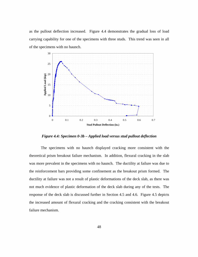
48
as the pullout deflection increased. Figure 4.4 demonstrates the gradual loss of load
carrying capability for one of the specimens with three studs. This trend was seen in all
of the specimens with no haunch.
0
5
10
15
20
25
30
0 0.1 0.2 0.3 0.4 0.5 0.6 0.7
Stud Pullout Deflection (in.)
App
lied
Loa
d (k
ip)
Figure 4.4: Specimen 0-3b – Applied load versus stud pullout deflection
The specimens with no haunch displayed cracking more consistent with the
theoretical prism breakout failure mechanism. In addition, flexural cracking in the slab
was more prevalent in the specimens with no haunch. The ductility at failure was due to
the reinforcement bars providing some confinement as the breakout prism formed. The
ductility at failure was not a result of plastic deformations of the deck slab, as there was
not much evidence of plastic deformation of the deck slab during any of the tests. The
response of the deck slab is discussed further in Section 4.5 and 4.6. Figure 4.5 depicts
the increased amount of flexural cracking and the cracking consistent with the breakout
failure mechanism.
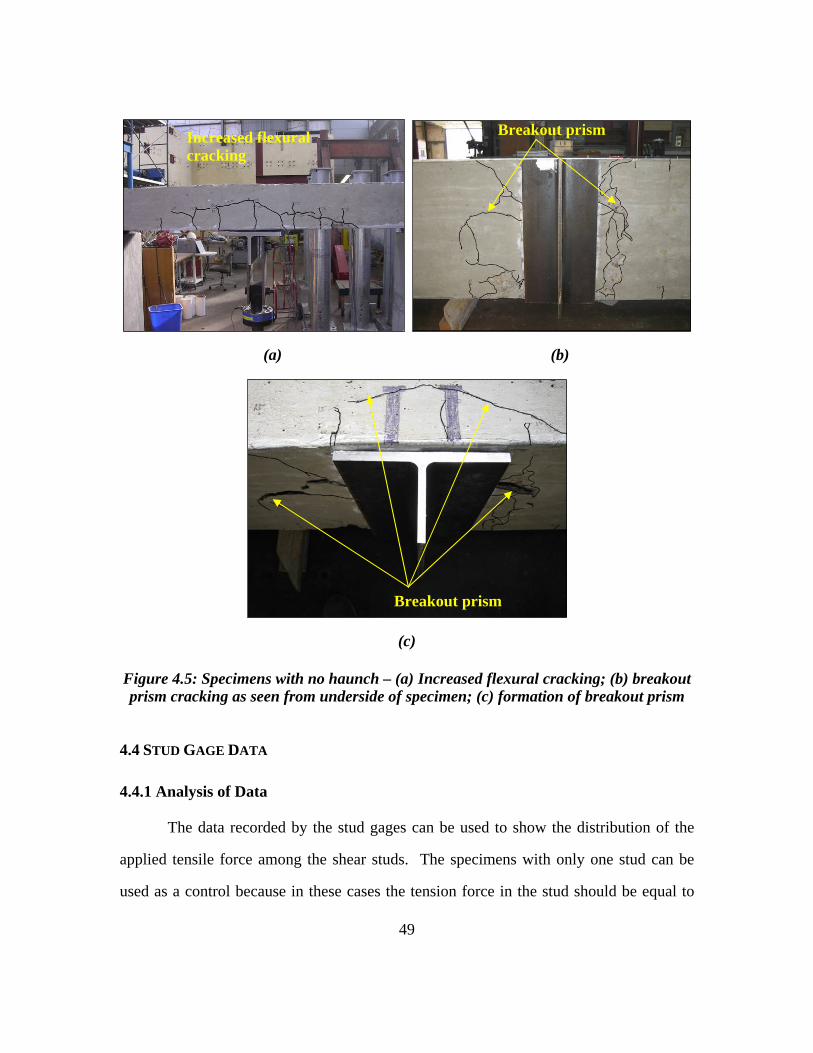
49
(a) (b)
(c)
Figure 4.5: Specimens with no haunch – (a) Increased flexural cracking; (b) breakout prism cracking as seen from underside of specimen; (c) formation of breakout prism
4.4 STUD GAGE DATA
4.4.1 Analysis of Data
The data recorded by the stud gages can be used to show the distribution of the
applied tensile force among the shear studs. The specimens with only one stud can be
used as a control because in these cases the tension force in the stud should be equal to
Increased flexural cracking
Breakout prism
Breakout prism
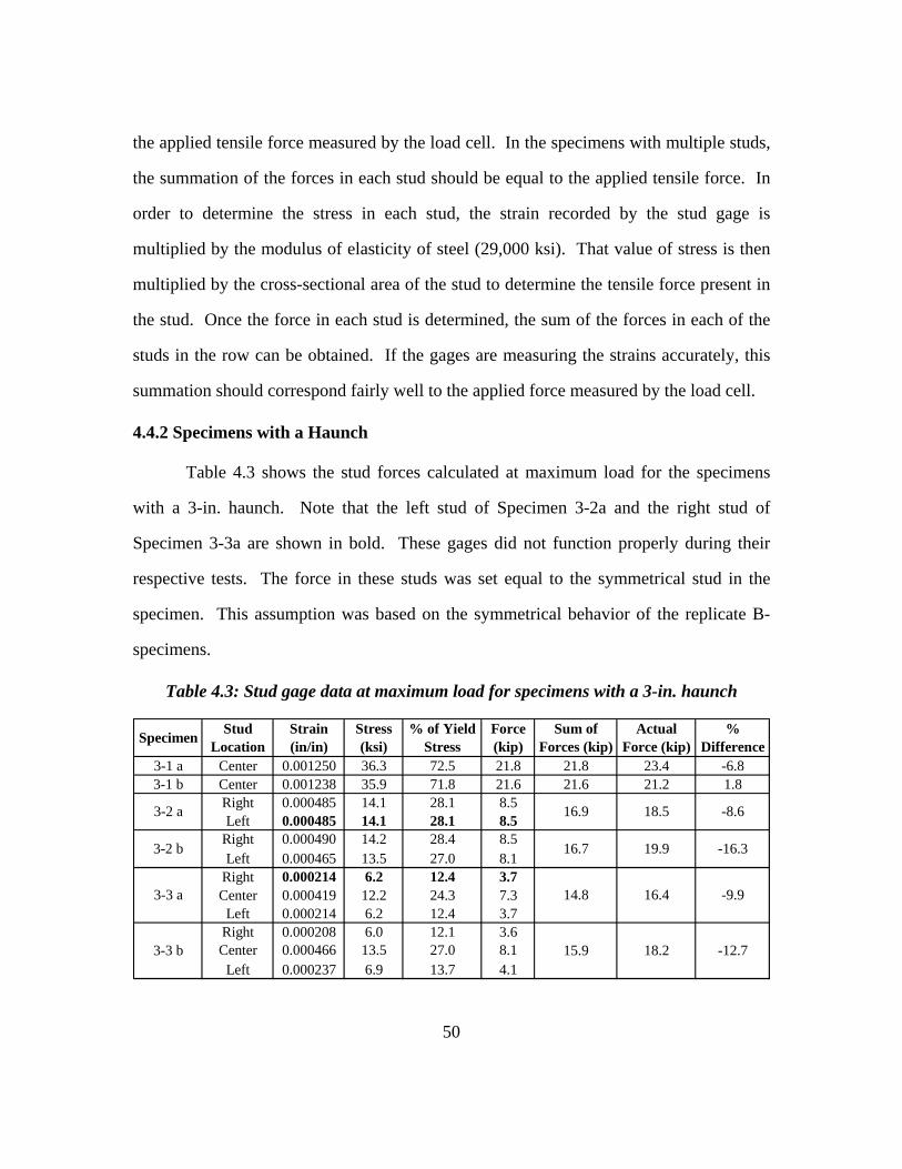
50
the applied tensile force measured by the load cell. In the specimens with multiple studs,
the summation of the forces in each stud should be equal to the applied tensile force. In
order to determine the stress in each stud, the strain recorded by the stud gage is
multiplied by the modulus of elasticity of steel (29,000 ksi). That value of stress is then
multiplied by the cross-sectional area of the stud to determine the tensile force present in
the stud. Once the force in each stud is determined, the sum of the forces in each of the
studs in the row can be obtained. If the gages are measuring the strains accurately, this
summation should correspond fairly well to the applied force measured by the load cell.
4.4.2 Specimens with a Haunch
Table 4.3 shows the stud forces calculated at maximum load for the specimens
with a 3-in. haunch. Note that the left stud of Specimen 3-2a and the right stud of
Specimen 3-3a are shown in bold. These gages did not function properly during their
respective tests. The force in these studs was set equal to the symmetrical stud in the
specimen. This assumption was based on the symmetrical behavior of the replicate B-
specimens.
Table 4.3: Stud gage data at maximum load for specimens with a 3-in. haunch
3-1 a Center 0.001250 36.3 72.5 21.8 21.8 23.4 -6.83-1 b Center 0.001238 35.9 71.8 21.6 21.6 21.2 1.8
Right 0.000485 14.1 28.1 8.5Left 0.000485 14.1 28.1 8.5
Right 0.000490 14.2 28.4 8.5Left 0.000465 13.5 27.0 8.1
Right 0.000214 6.2 12.4 3.7Center 0.000419 12.2 24.3 7.3
Left 0.000214 6.2 12.4 3.7Right 0.000208 6.0 12.1 3.6Center 0.000466 13.5 27.0 8.1
Left 0.000237 6.9 13.7 4.1
% Difference
% of Yield Stress
Force (kip)
Sum of Forces (kip)
Actual Force (kip)Specimen Stud
LocationStrain (in/in)
Stress (ksi)
-12.7
-9.9
-16.3
-8.6
3-3 b
3-3 a
3-2 b
3-2 a
15.9 18.2
16.9 18.5
19.916.7
14.8 16.4
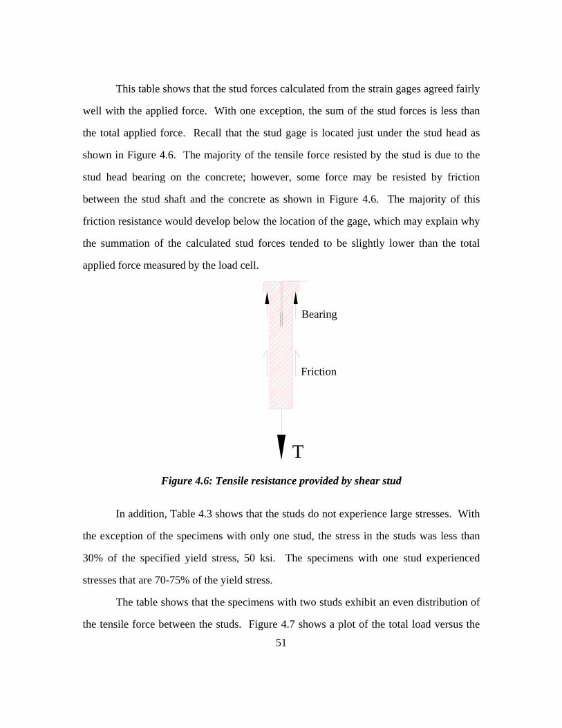
51
This table shows that the stud forces calculated from the strain gages agreed fairly
well with the applied force. With one exception, the sum of the stud forces is less than
the total applied force. Recall that the stud gage is located just under the stud head as
shown in Figure 4.6. The majority of the tensile force resisted by the stud is due to the
stud head bearing on the concrete; however, some force may be resisted by friction
between the stud shaft and the concrete as shown in Figure 4.6. The majority of this
friction resistance would develop below the location of the gage, which may explain why
the summation of the calculated stud forces tended to be slightly lower than the total
applied force measured by the load cell.
T
Bearing
Friction
Figure 4.6: Tensile resistance provided by shear stud
In addition, Table 4.3 shows that the studs do not experience large stresses. With
the exception of the specimens with only one stud, the stress in the studs was less than
30% of the specified yield stress, 50 ksi. The specimens with one stud experienced
stresses that are 70-75% of the yield stress.
The table shows that the specimens with two studs exhibit an even distribution of
the tensile force between the studs. Figure 4.7 shows a plot of the total load versus the
52
calculated force in the studs for Specimen 3-2b, which has a 3-in. haunch and two studs.
The force in each of the two studs is nearly identical throughout the entire test up until
failure.
0
5
10
15
20
25
0 1 2 3 4 5 6 7 8 9
Stud Force (kip)
Tot
al A
pplie
d Fo
rce
(kip
)
Left Stud
Right Stud
Figure 4.7: Specimen 3-2b – Applied load versus calculated force in the shear studs
The stud gages in the specimens with three studs showed that approximately half
of the applied tensile force is resisted by the center stud and that the remaining half is
equally distributed between the two outer studs. Figure 4.8 shows a plot of the applied
load versus the calculated force in the studs for a specimen with three studs. This plot
shows that the force in the three studs is fairly uniform until approximately 7 kips, after
which the center stud begins to resist a very large portion of the applied load. This point
represents the cracking load of the slab (See Section 4.5.1). The slab cracks first at the
haunch edges, which is very close to the outside studs. The slab did not crack inside the
haunch region. Therefore, the center stud begins to resist more force after cracking
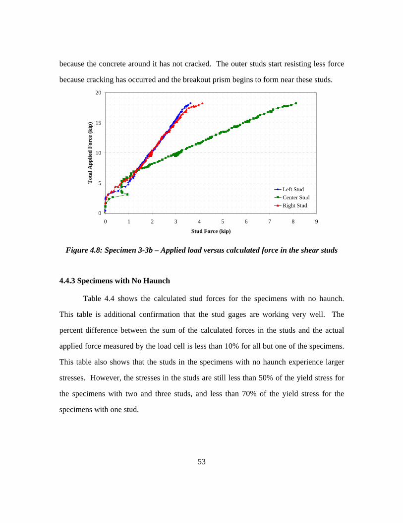
53
because the concrete around it has not cracked. The outer studs start resisting less force
because cracking has occurred and the breakout prism begins to form near these studs.
0
5
10
15
20
0 1 2 3 4 5 6 7 8 9
Stud Force (kip)
Tot
al A
pplie
d Fo
rce
(kip
)
Left StudCenter StudRight Stud
Figure 4.8: Specimen 3-3b – Applied load versus calculated force in the shear studs
4.4.3 Specimens with No Haunch
Table 4.4 shows the calculated stud forces for the specimens with no haunch.
This table is additional confirmation that the stud gages are working very well. The
percent difference between the sum of the calculated forces in the studs and the actual
applied force measured by the load cell is less than 10% for all but one of the specimens.
This table also shows that the studs in the specimens with no haunch experience larger
stresses. However, the stresses in the studs are still less than 50% of the yield stress for
the specimens with two and three studs, and less than 70% of the yield stress for the
specimens with one stud.
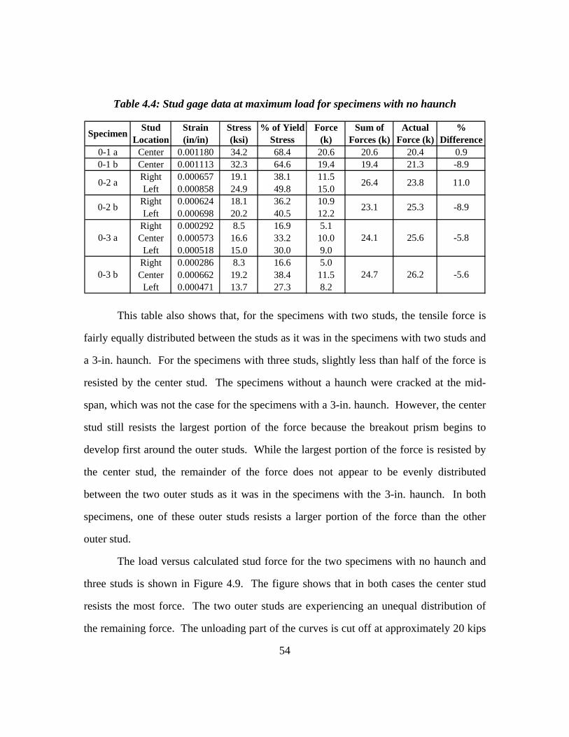
54
Table 4.4: Stud gage data at maximum load for specimens with no haunch
0-1 a Center 0.001180 34.2 68.4 20.6 20.6 20.4 0.90-1 b Center 0.001113 32.3 64.6 19.4 19.4 21.3 -8.9
Right 0.000657 19.1 38.1 11.5Left 0.000858 24.9 49.8 15.0
Right 0.000624 18.1 36.2 10.9Left 0.000698 20.2 40.5 12.2
Right 0.000292 8.5 16.9 5.1Center 0.000573 16.6 33.2 10.0
Left 0.000518 15.0 30.0 9.0Right 0.000286 8.3 16.6 5.0Center 0.000662 19.2 38.4 11.5
Left 0.000471 13.7 27.3 8.2
Stud Location
Strain (in/in)
Stress (ksi)
% Difference
0-2 a 26.4 23.8 11.0
% of Yield Stress
Force (k)
Sum of Forces (k)
Actual Force (k)Specimen
0-2 b 23.1 25.3 -8.9
0-3 a 24.1 25.6 -5.8
0-3 b 24.7 26.2 -5.6
This table also shows that, for the specimens with two studs, the tensile force is
fairly equally distributed between the studs as it was in the specimens with two studs and
a 3-in. haunch. For the specimens with three studs, slightly less than half of the force is
resisted by the center stud. The specimens without a haunch were cracked at the mid-
span, which was not the case for the specimens with a 3-in. haunch. However, the center
stud still resists the largest portion of the force because the breakout prism begins to
develop first around the outer studs. While the largest portion of the force is resisted by
the center stud, the remainder of the force does not appear to be evenly distributed
between the two outer studs as it was in the specimens with the 3-in. haunch. In both
specimens, one of these outer studs resists a larger portion of the force than the other
outer stud.
The load versus calculated stud force for the two specimens with no haunch and
three studs is shown in Figure 4.9. The figure shows that in both cases the center stud
resists the most force. The two outer studs are experiencing an unequal distribution of
the remaining force. The unloading part of the curves is cut off at approximately 20 kips
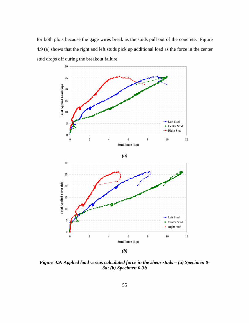
55
for both plots because the gage wires break as the studs pull out of the concrete. Figure
4.9 (a) shows that the right and left studs pick up additional load as the force in the center
stud drops off during the breakout failure.
0
5
10
15
20
25
30
0 2 4 6 8 10 12
Stud Force (kip)
Tot
al A
pplie
d L
oad
(kip
)
Left StudCenter StudRight Stud
(a)
0
5
10
15
20
25
30
0 2 4 6 8 10 12
Stud Force (kip)
Tot
al A
pplie
d Fo
rce
(kip
)
Left StudCenter StudRight Stud
(b)
Figure 4.9: Applied load versus calculated force in the shear studs – (a) Specimen 0-3a; (b) Specimen 0-3b
56
4.5 REINFORCING STEEL GAGE DATA
4.5.1 Concrete Slab – Cracking, Yielding, and Ultimate Loads
The data obtained from the strain gages on the reinforcing steel show how the slab
is behaving during each test. The three important stages of each test, in terms of the
concrete slab, are the loads that correspond to cracking, yielding, and ultimate. The loads
corresponding to each of these points was calculated in order to see if the actual behavior
matched the assumed behavior.
Each slab was simply supported, and the ram pulled down on the WT section,
loading the studs in tension and the slab in bending. Therefore, it can be assumed that
each specimen is a simply supported slab with a point load at mid-span. From simple
statics, the moment at the mid-span and the quarter-span is equal to PL/4 and PL/8,
respectively, where P is the applied tensile force and L is the span length of the slab.
Using this relationship between applied load and moment, the expected cracking load,
yield load, and ultimate load can be determined.
The calculation of the cracking moment, yield moment, and ultimate moment was
based on a concrete strength of 6 ksi, steel reinforcement yield strength of 60 ksi, and a
slab thickness of 8 in. This concrete strength was used because it corresponds to the
strength of the concrete cylinders halfway through the testing period (See Section 4.7). A
tension test on a reinforcement bar also confirmed that 60 ksi was an acceptable value to
use for the yield strength of the reinforcement. The extra depth in the haunch region was
not included in these calculations, and the calculations also assumed that the applied
force was uniformly distributed throughout the width of the slab. See Appendix D for
actual calculations of each value.
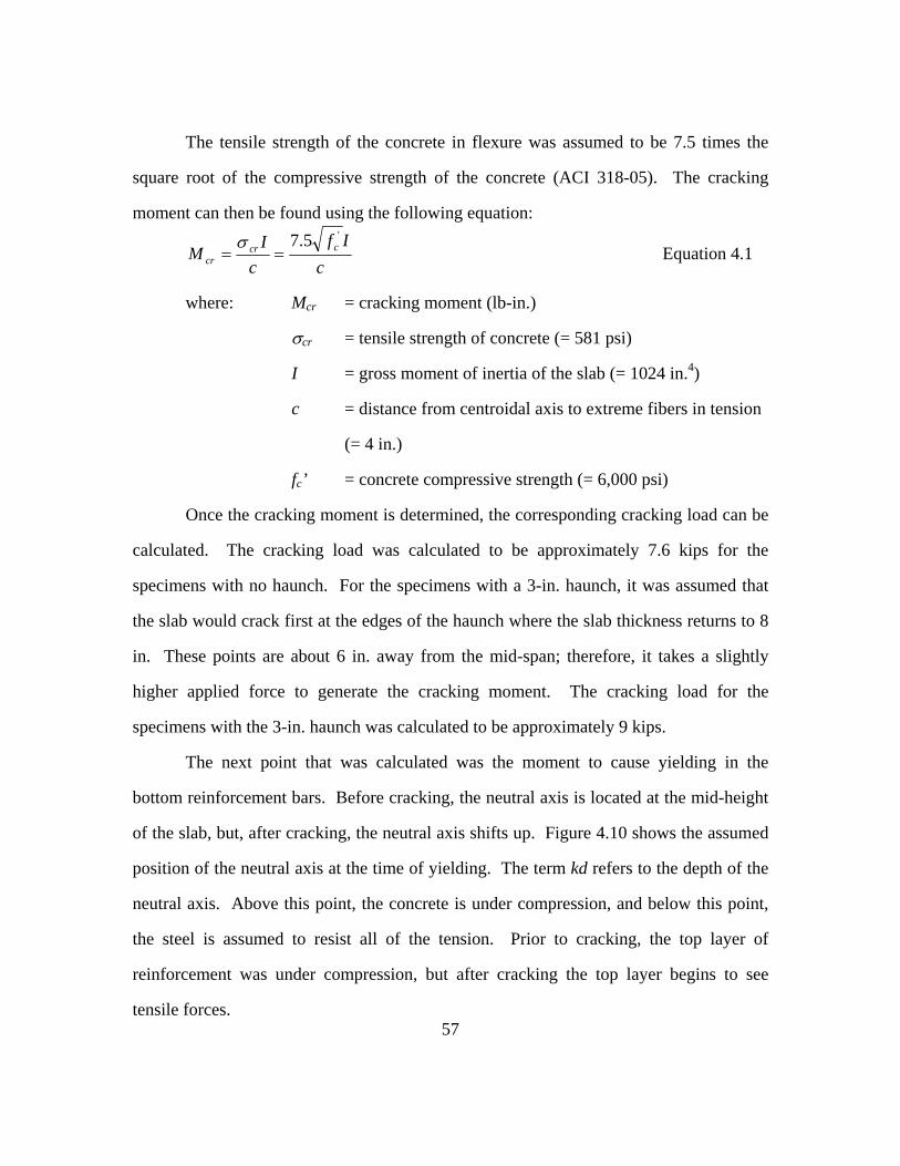
57
The tensile strength of the concrete in flexure was assumed to be 7.5 times the
square root of the compressive strength of the concrete (ACI 318-05). The cracking
moment can then be found using the following equation:
cIf
cI
M ccrcr
'5.7==
σ Equation 4.1
where: Mcr = cracking moment (lb-in.)
σcr = tensile strength of concrete (= 581 psi)
I = gross moment of inertia of the slab (= 1024 in.4)
c = distance from centroidal axis to extreme fibers in tension
(= 4 in.)
fc’ = concrete compressive strength (= 6,000 psi)
Once the cracking moment is determined, the corresponding cracking load can be
calculated. The cracking load was calculated to be approximately 7.6 kips for the
specimens with no haunch. For the specimens with a 3-in. haunch, it was assumed that
the slab would crack first at the edges of the haunch where the slab thickness returns to 8
in. These points are about 6 in. away from the mid-span; therefore, it takes a slightly
higher applied force to generate the cracking moment. The cracking load for the
specimens with the 3-in. haunch was calculated to be approximately 9 kips.
The next point that was calculated was the moment to cause yielding in the
bottom reinforcement bars. Before cracking, the neutral axis is located at the mid-height
of the slab, but, after cracking, the neutral axis shifts up. Figure 4.10 shows the assumed
position of the neutral axis at the time of yielding. The term kd refers to the depth of the
neutral axis. Above this point, the concrete is under compression, and below this point,
the steel is assumed to resist all of the tension. Prior to cracking, the top layer of
reinforcement was under compression, but after cracking the top layer begins to see
tensile forces.
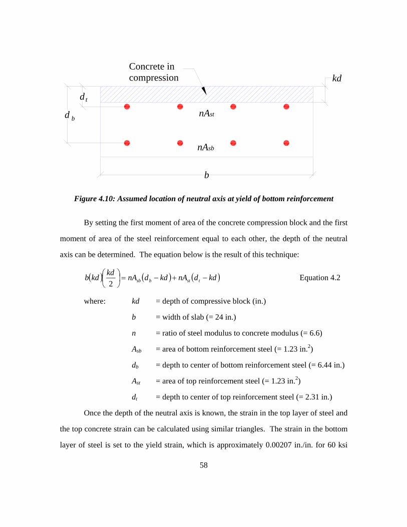
58
kdConcrete in compression
d
d b
t
nAsb
nAst
b
Figure 4.10: Assumed location of neutral axis at yield of bottom reinforcement
By setting the first moment of area of the concrete compression block and the first
moment of area of the steel reinforcement equal to each other, the depth of the neutral
axis can be determined. The equation below is the result of this technique:
( ) ( ) ( )kddnAkddnAkdkdb tstbsb −+−=⎟⎠⎞
⎜⎝⎛
2 Equation 4.2
where: kd = depth of compressive block (in.)
b = width of slab (= 24 in.)
n = ratio of steel modulus to concrete modulus (= 6.6)
Asb = area of bottom reinforcement steel (= 1.23 in.2)
db = depth to center of bottom reinforcement steel (= 6.44 in.)
Ast = area of top reinforcement steel (= 1.23 in.2)
dt = depth to center of top reinforcement steel (= 2.31 in.)
Once the depth of the neutral axis is known, the strain in the top layer of steel and
the top concrete strain can be calculated using similar triangles. The strain in the bottom
layer of steel is set to the yield strain, which is approximately 0.00207 in./in. for 60 ksi
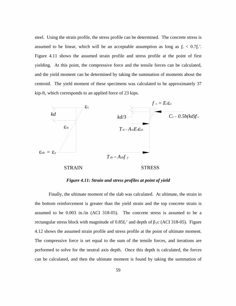
59
steel. Using the strain profile, the stress profile can be determined. The concrete stress is
assumed to be linear, which will be an acceptable assumption as long as fc < 0.7fc’.
Figure 4.11 shows the assumed strain profile and stress profile at the point of first
yielding. At this point, the compressive force and the tensile forces can be calculated,
and the yield moment can be determined by taking the summation of moments about the
centroid. The yield moment of these specimens was calculated to be approximately 37
kip-ft, which corresponds to an applied force of 23 kips.
εsb = εy
εst
εc
kd
Tsb = Asbf y
kd/3
Tst = AstEsεst
f c = Ecεc
Cc = 0.5b(kd)f c
STRAIN STRESS
Figure 4.11: Strain and stress profiles at point of yield
Finally, the ultimate moment of the slab was calculated. At ultimate, the strain in
the bottom reinforcement is greater than the yield strain and the top concrete strain is
assumed to be 0.003 in./in (ACI 318-05). The concrete stress is assumed to be a
rectangular stress block with magnitude of 0.85fc’ and depth of β1c (ACI 318-05). Figure
4.12 shows the assumed strain profile and stress profile at the point of ultimate moment.
The compressive force is set equal to the sum of the tensile forces, and iterations are
performed to solve for the neutral axis depth. Once this depth is calculated, the forces
can be calculated, and then the ultimate moment is found by taking the summation of
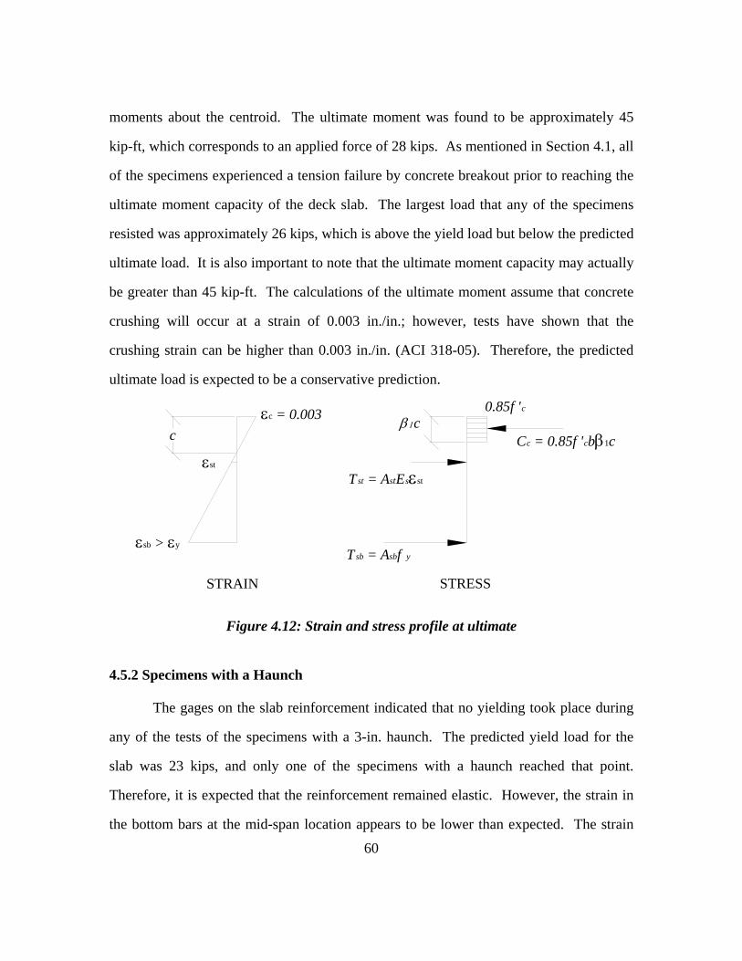
60
moments about the centroid. The ultimate moment was found to be approximately 45
kip-ft, which corresponds to an applied force of 28 kips. As mentioned in Section 4.1, all
of the specimens experienced a tension failure by concrete breakout prior to reaching the
ultimate moment capacity of the deck slab. The largest load that any of the specimens
resisted was approximately 26 kips, which is above the yield load but below the predicted
ultimate load. It is also important to note that the ultimate moment capacity may actually
be greater than 45 kip-ft. The calculations of the ultimate moment assume that concrete
crushing will occur at a strain of 0.003 in./in.; however, tests have shown that the
crushing strain can be higher than 0.003 in./in. (ACI 318-05). Therefore, the predicted
ultimate load is expected to be a conservative prediction.
εsb > εy
εst
εc = 0.003 c
Tsb = Asbf y
Tst = AstEsεst
0.85f 'c
Cc = 0.85f 'cbβ1c
STRAIN STRESS
β 1c
Figure 4.12: Strain and stress profile at ultimate
4.5.2 Specimens with a Haunch
The gages on the slab reinforcement indicated that no yielding took place during
any of the tests of the specimens with a 3-in. haunch. The predicted yield load for the
slab was 23 kips, and only one of the specimens with a haunch reached that point.
Therefore, it is expected that the reinforcement remained elastic. However, the strain in
the bottom bars at the mid-span location appears to be lower than expected. The strain
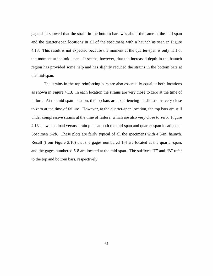
61
gage data showed that the strain in the bottom bars was about the same at the mid-span
and the quarter-span locations in all of the specimens with a haunch as seen in Figure
4.13. This result is not expected because the moment at the quarter-span is only half of
the moment at the mid-span. It seems, however, that the increased depth in the haunch
region has provided some help and has slightly reduced the strains in the bottom bars at
the mid-span.
The strains in the top reinforcing bars are also essentially equal at both locations
as shown in Figure 4.13. In each location the strains are very close to zero at the time of
failure. At the mid-span location, the top bars are experiencing tensile strains very close
to zero at the time of failure. However, at the quarter-span location, the top bars are still
under compressive strains at the time of failure, which are also very close to zero. Figure
4.13 shows the load versus strain plots at both the mid-span and quarter-span locations of
Specimen 3-2b. These plots are fairly typical of all the specimens with a 3-in. haunch.
Recall (from Figure 3.10) that the gages numbered 1-4 are located at the quarter-span,
and the gages numbered 5-8 are located at the mid-span. The suffixes “T” and “B” refer
to the top and bottom bars, respectively.
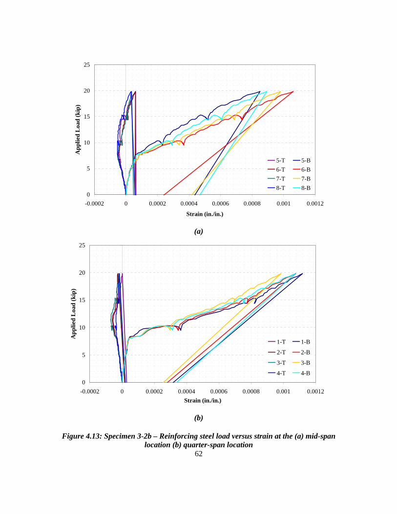
62
0
5
10
15
20
25
-0.0002 0 0.0002 0.0004 0.0006 0.0008 0.001 0.0012
Strain (in./in.)
App
lied
Loa
d (k
ip)
5-T 5-B6-T 6-B7-T 7-B8-T 8-B
(a)
0
5
10
15
20
25
-0.0002 0 0.0002 0.0004 0.0006 0.0008 0.001 0.0012Strain (in./in.)
App
lied
Loa
d (k
ip)
1-T 1-B
2-T 2-B
3-T 3-B
4-T 4-B
(b)
Figure 4.13: Specimen 3-2b – Reinforcing steel load versus strain at the (a) mid-span location (b) quarter-span location
63
Initially the slope of the load versus strain curves is very steep, but around 8 kips
the slope decreases drastically. This point represents the cracking load, which is very
close to the predicted cracking load of 9 kips for the specimens with a haunch. After
cracking, the section becomes much less stiff, and the strain increases at a faster rate.
These plots also show that the top bars start off in compression (represented by a negative
strain), but after cracking they go into tension as the neutral axis shifts upwards.
4.5.3 Specimens with No Haunch
For the specimens with no haunch, the gages on the reinforcement indicated that
yielding of the bottom bars at the mid-span occurred in all specimens. The predicted
yield load for these specimens was about 23 kips, but, based upon the strain gage
readings, all of the bottom reinforcement reached the yield strain even though only four
of the six specimens resisted a load greater than 23 kips. However, the strain in these
bars was typically just barely above the yield strain at the time of the breakout failure.
The strains were not large enough in any of these specimens to produce noticeable plastic
deformation of the slab. Figure 4.14 shows a typical load versus strain plot for a
specimen with no haunch in which all of the bottom bars have reached the theoretical
yield strain of 0.00207 in./in.
64
0
5
10
15
20
25
-0.0005 0 0.0005 0.001 0.0015 0.002 0.0025 0.003Strain (in./in.)
App
lied
Loa
d (k
ip)
5-T 5-B6-T 6-B7-T 7-B8-T 8-Bεy
Figure 4.14: Specimen 0-2a – Mid-span reinforcing steel load versus strain
Although the bottom bars have all reached the yield strain, the load continues to
increase after this point. This happens because of the presence of the top layer of
reinforcement in the slab. The bottom bars have yielded, but the top bars have not, so the
slab can continue to resist additional load. The plot also shows that the cracking load is
between 5 and 6 kips, which is slightly less than the predicted cracking load of 7.6 kips.
In a couple of the specimens with no haunch, a significant amount of yielding
occurred in one or two of the bottom bars at the mid-span. Figure 4.15 shows one of
these specimens. The two bars that have yielded significantly are 5-B and 8-B, which
correspond to the outer bars. As the breakout prism forms in the center of the slab, and
the bond between the middle bars and the concrete is lost, it seems that the strain is
redistributed to the outer bars that are not affected by the breakout prism.
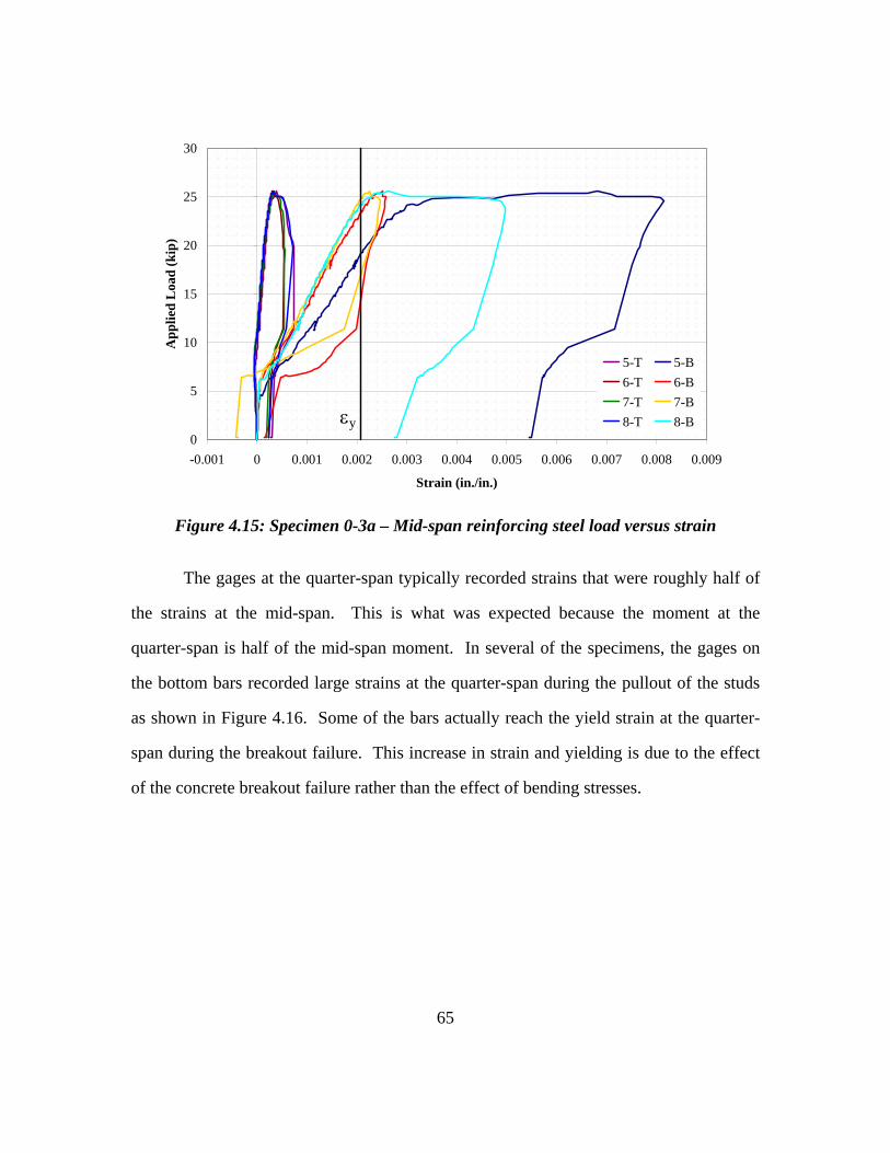
65
0
5
10
15
20
25
30
-0.001 0 0.001 0.002 0.003 0.004 0.005 0.006 0.007 0.008 0.009
Strain (in./in.)
App
lied
Loa
d (k
ip)
5-T 5-B6-T 6-B7-T 7-B8-T 8-Bεy
Figure 4.15: Specimen 0-3a – Mid-span reinforcing steel load versus strain
The gages at the quarter-span typically recorded strains that were roughly half of
the strains at the mid-span. This is what was expected because the moment at the
quarter-span is half of the mid-span moment. In several of the specimens, the gages on
the bottom bars recorded large strains at the quarter-span during the pullout of the studs
as shown in Figure 4.16. Some of the bars actually reach the yield strain at the quarter-
span during the breakout failure. This increase in strain and yielding is due to the effect
of the concrete breakout failure rather than the effect of bending stresses.
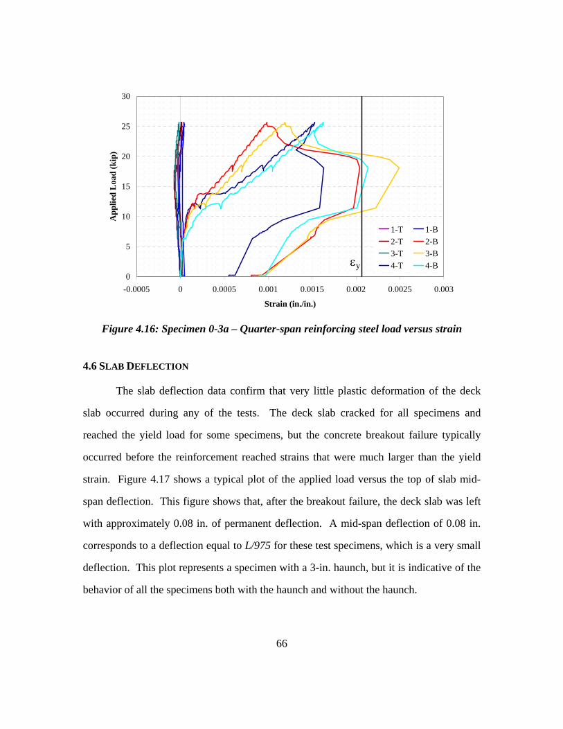
66
0
5
10
15
20
25
30
-0.0005 0 0.0005 0.001 0.0015 0.002 0.0025 0.003
Strain (in./in.)
App
lied
Loa
d (k
ip)
1-T 1-B2-T 2-B3-T 3-B4-T 4-Bεy
Figure 4.16: Specimen 0-3a – Quarter-span reinforcing steel load versus strain
4.6 SLAB DEFLECTION
The slab deflection data confirm that very little plastic deformation of the deck
slab occurred during any of the tests. The deck slab cracked for all specimens and
reached the yield load for some specimens, but the concrete breakout failure typically
occurred before the reinforcement reached strains that were much larger than the yield
strain. Figure 4.17 shows a typical plot of the applied load versus the top of slab mid-
span deflection. This figure shows that, after the breakout failure, the deck slab was left
with approximately 0.08 in. of permanent deflection. A mid-span deflection of 0.08 in.
corresponds to a deflection equal to L/975 for these test specimens, which is a very small
deflection. This plot represents a specimen with a 3-in. haunch, but it is indicative of the
behavior of all the specimens both with the haunch and without the haunch.

67
0
5
10
15
20
0 0.02 0.04 0.06 0.08 0.1 0.12 0.14 0.16
Top of Slab Deflection (in.)
App
lied
Loa
d (k
ip)
Figure 4.17: Specimen 3-3a – Typical load versus top of slab deflection plot
Figure 4.17 shows that the specimen is initially very stiff, but then it becomes
much less stiff at about 5 or 6 kips. This point represents the cracking load, which was
predicted in Section 4.5.1 to be approximately 8-9 kips. Prior to cracking, the section
behaves with gross section properties, making the moment of inertia much greater and the
slab much stiffer than a cracked slab. After the section cracks, the cracked section
properties dictate the behavior and so the specimen is less stiff.
Another interesting point shown in this plot is the V-notch seen at about 10 kips.
This is a point at which the loading was paused to map cracks and inspect the specimen.
The deflection is held constant by the ram, and the load drops off slightly. The loading
rate during a test is considered to be an intermediate loading rate, which is between a
static and dynamic loading rate. The V-notch point represents a static value on the load
versus deflection plot. These V-notches can also be seen in previous sections on the
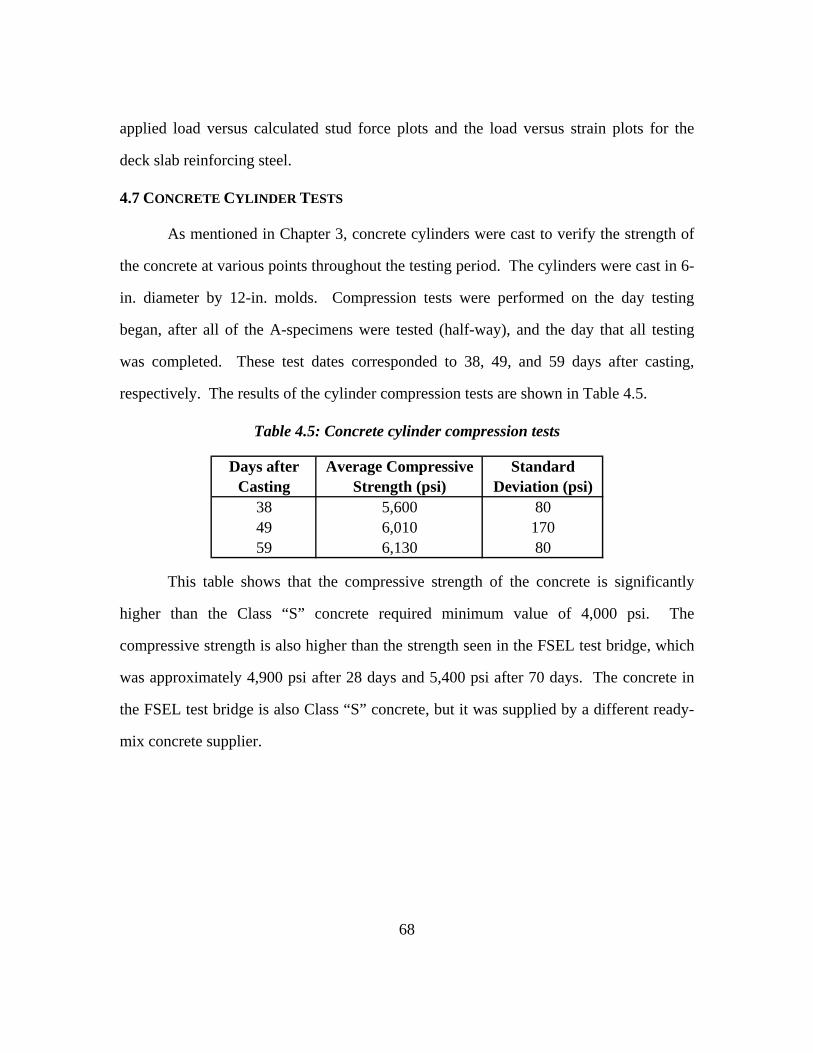
68
applied load versus calculated stud force plots and the load versus strain plots for the
deck slab reinforcing steel.
4.7 CONCRETE CYLINDER TESTS
As mentioned in Chapter 3, concrete cylinders were cast to verify the strength of
the concrete at various points throughout the testing period. The cylinders were cast in 6-
in. diameter by 12-in. molds. Compression tests were performed on the day testing
began, after all of the A-specimens were tested (half-way), and the day that all testing
was completed. These test dates corresponded to 38, 49, and 59 days after casting,
respectively. The results of the cylinder compression tests are shown in Table 4.5.
Table 4.5: Concrete cylinder compression tests
38 5,600 8049 6,010 17059 6,130 80
Standard Deviation (psi)
Average Compressive Strength (psi)
Days after Casting
This table shows that the compressive strength of the concrete is significantly
higher than the Class “S” concrete required minimum value of 4,000 psi. The
compressive strength is also higher than the strength seen in the FSEL test bridge, which
was approximately 4,900 psi after 28 days and 5,400 psi after 70 days. The concrete in
the FSEL test bridge is also Class “S” concrete, but it was supplied by a different ready-
mix concrete supplier.
69
CHAPTER 5
Analysis and Discussion of Test Results
5.1 PREDICTED CAPACITIES VERSUS TEST RESULTS
Using the equations found in Appendix D of the ACI 318 code, a predicted tensile
capacity for each of the six unique specimens was calculated. In calculating the predicted
values, the governing failure mode for all specimens was concrete breakout. The
predicted values are based on a concrete compressive strength of 6,000 psi. This concrete
strength was chosen because it corresponds to the strength of the concrete cylinders at the
midway point of the testing program. Strength reduction factors (φ) were not applied to
the predicted values. The detailed calculations of the predicted capacity of each
specimen are given in Appendix E.
As described in detail in Chapter 2, the equations used to calculate the concrete
breakout strength are as follows:
5.1'efccb hfkN = Equation 5.1 (ACI 318-05)
bNcNedNecNco
Nccbg N
AA
N ,,, ψψψ= Equation 5.2 (ACI 318-05)
where: Nb = concrete breakout strength of a single anchor in cracked
concrete with no edge or group effects (lb)
kc = 24 for cast-in anchors
fc’ = specified compressive strength of concrete (psi)
hef = effective anchor embedment depth (in.)
Ncbg = concrete breakout strength of an anchor or group of
anchors (lb)
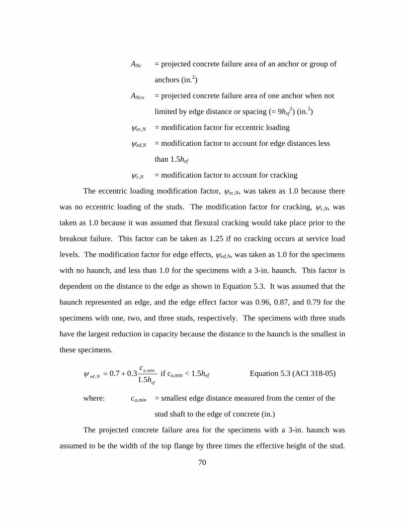
70
ANc = projected concrete failure area of an anchor or group of
anchors (in.2)
ANco = projected concrete failure area of one anchor when not
limited by edge distance or spacing (= 9hef2) (in.2)
ψec,N = modification factor for eccentric loading
ψed,N = modification factor to account for edge distances less
than 1.5hef
ψc,N = modification factor to account for cracking
The eccentric loading modification factor, ψec,N, was taken as 1.0 because there
was no eccentric loading of the studs. The modification factor for cracking, ψc,N, was
taken as 1.0 because it was assumed that flexural cracking would take place prior to the
breakout failure. This factor can be taken as 1.25 if no cracking occurs at service load
levels. The modification factor for edge effects, ψed,N, was taken as 1.0 for the specimens
with no haunch, and less than 1.0 for the specimens with a 3-in. haunch. This factor is
dependent on the distance to the edge as shown in Equation 5.3. It was assumed that the
haunch represented an edge, and the edge effect factor was 0.96, 0.87, and 0.79 for the
specimens with one, two, and three studs, respectively. The specimens with three studs
have the largest reduction in capacity because the distance to the haunch is the smallest in
these specimens.
ef
aNed h
c5.1
3.07.0 min,, +=ψ if ca,min < 1.5hef Equation 5.3 (ACI 318-05)
where: ca,min = smallest edge distance measured from the center of the
stud shaft to the edge of concrete (in.)
The projected concrete failure area for the specimens with a 3-in. haunch was
assumed to be the width of the top flange by three times the effective height of the stud.
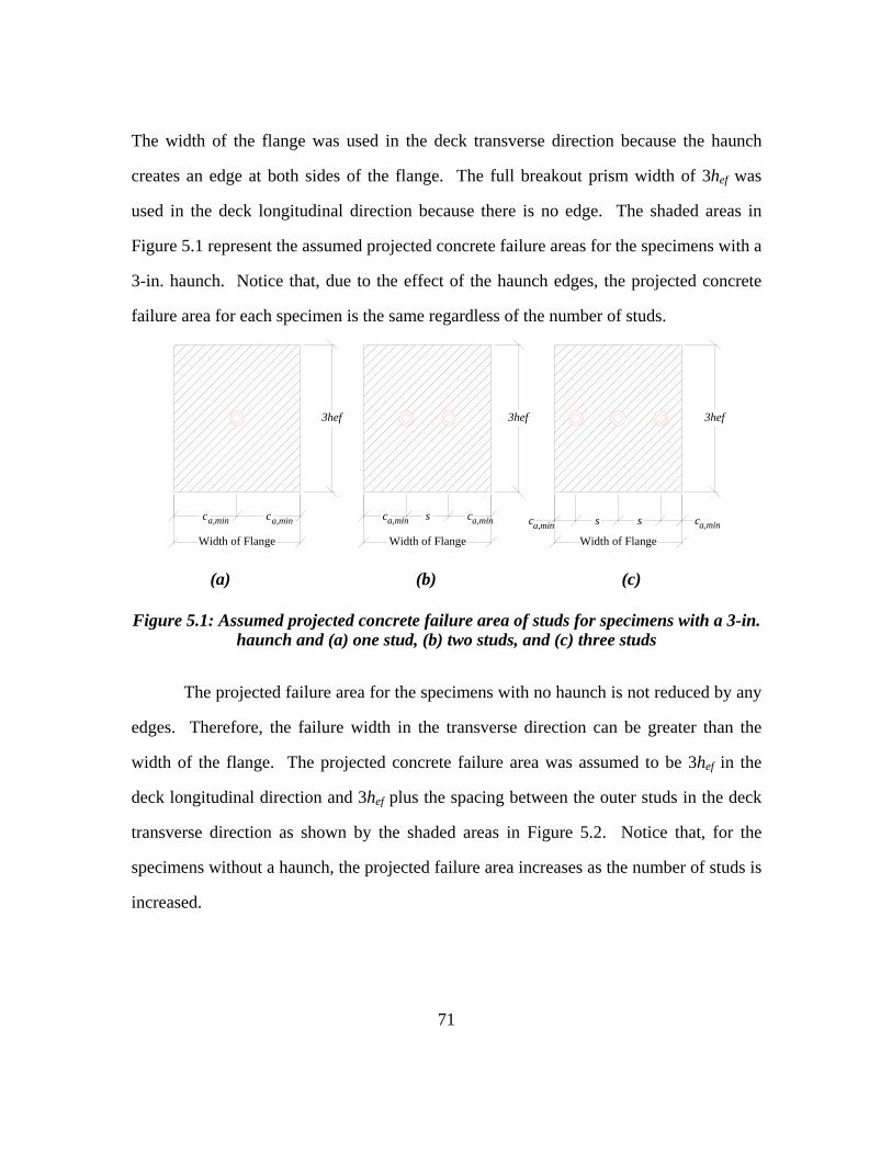
71
The width of the flange was used in the deck transverse direction because the haunch
creates an edge at both sides of the flange. The full breakout prism width of 3hef was
used in the deck longitudinal direction because there is no edge. The shaded areas in
Figure 5.1 represent the assumed projected concrete failure areas for the specimens with a
3-in. haunch. Notice that, due to the effect of the haunch edges, the projected concrete
failure area for each specimen is the same regardless of the number of studs.
3hef
s sc c
3hef
s cc
3hef
cc
Width of Flange Width of Flange Width of Flange
a,min a,min a,min a,min a,min a,min
(a) (b) (c)
Figure 5.1: Assumed projected concrete failure area of studs for specimens with a 3-in. haunch and (a) one stud, (b) two studs, and (c) three studs
The projected failure area for the specimens with no haunch is not reduced by any
edges. Therefore, the failure width in the transverse direction can be greater than the
width of the flange. The projected concrete failure area was assumed to be 3hef in the
deck longitudinal direction and 3hef plus the spacing between the outer studs in the deck
transverse direction as shown by the shaded areas in Figure 5.2. Notice that, for the
specimens without a haunch, the projected failure area increases as the number of studs is
increased.
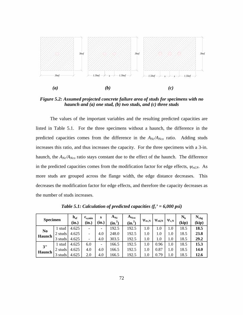
72
3hef
s s1.5hef 1.5hef
3hef
s 1.5hef1.5hef
3hef
3hef
(a) (b) (c)
Figure 5.2: Assumed projected concrete failure area of studs for specimens with no haunch and (a) one stud, (b) two studs, and (c) three studs
The values of the important variables and the resulting predicted capacities are
listed in Table 5.1. For the three specimens without a haunch, the difference in the
predicted capacities comes from the difference in the ANc/ANco ratio. Adding studs
increases this ratio, and thus increases the capacity. For the three specimens with a 3-in.
haunch, the ANc/ANco ratio stays constant due to the effect of the haunch. The difference
in the predicted capacities comes from the modification factor for edge effects, ψed,N. As
more studs are grouped across the flange width, the edge distance decreases. This
decreases the modification factor for edge effects, and therefore the capacity decreases as
the number of studs increases.
Table 5.1: Calculation of predicted capacities (fc’ = 6,000 psi)
1 stud 4.625 - - 192.5 192.5 1.0 1.0 1.0 18.5 18.52 studs 4.625 - 4.0 248.0 192.5 1.0 1.0 1.0 18.5 23.83 studs 4.625 - 4.0 303.5 192.5 1.0 1.0 1.0 18.5 29.21 stud 4.625 6.0 - 166.5 192.5 1.0 0.96 1.0 18.5 15.32 studs 4.625 4.0 4.0 166.5 192.5 1.0 0.87 1.0 18.5 14.03 studs 4.625 2.0 4.0 166.5 192.5 1.0 0.79 1.0 18.5 12.6
ca,min
(in.)hef
(in.)ψec,N
ANco
(in.2)ANc
(in.2)s
(in.)Ncbg
(kip)Nb
(kip)ψc,Nψed,N
No Haunch
3" Haunch
Specimen
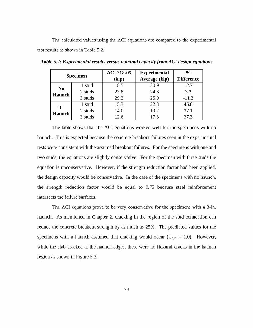
73
The calculated values using the ACI equations are compared to the experimental
test results as shown in Table 5.2.
Table 5.2: Experimental results versus nominal capacity from ACI design equations
1 stud 18.5 20.9 12.72 studs 23.8 24.6 3.23 studs 29.2 25.9 -11.31 stud 15.3 22.3 45.82 studs 14.0 19.2 37.13 studs 12.6 17.3 37.3
3" Haunch
Specimen % Difference
ACI 318-05 (kip)
Experimental Average (kip)
No Haunch
The table shows that the ACI equations worked well for the specimens with no
haunch. This is expected because the concrete breakout failures seen in the experimental
tests were consistent with the assumed breakout failures. For the specimens with one and
two studs, the equations are slightly conservative. For the specimen with three studs the
equation is unconservative. However, if the strength reduction factor had been applied,
the design capacity would be conservative. In the case of the specimens with no haunch,
the strength reduction factor would be equal to 0.75 because steel reinforcement
intersects the failure surfaces.
The ACI equations prove to be very conservative for the specimens with a 3-in.
haunch. As mentioned in Chapter 2, cracking in the region of the stud connection can
reduce the concrete breakout strength by as much as 25%. The predicted values for the
specimens with a haunch assumed that cracking would occur (ψc,N = 1.0). However,
while the slab cracked at the haunch edges, there were no flexural cracks in the haunch
region as shown in Figure 5.3.
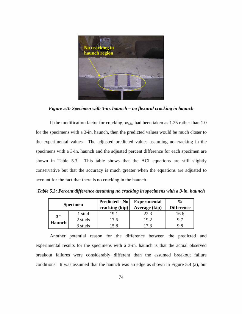
74
Figure 5.3: Specimen with 3-in. haunch – no flexural cracking in haunch
If the modification factor for cracking, ψc,N, had been taken as 1.25 rather than 1.0
for the specimens with a 3-in. haunch, then the predicted values would be much closer to
the experimental values. The adjusted predicted values assuming no cracking in the
specimens with a 3-in. haunch and the adjusted percent difference for each specimen are
shown in Table 5.3. This table shows that the ACI equations are still slightly
conservative but that the accuracy is much greater when the equations are adjusted to
account for the fact that there is no cracking in the haunch.
Table 5.3: Percent difference assuming no cracking in specimens with a 3-in. haunch
1 stud 19.1 22.3 16.62 studs 17.5 19.2 9.73 studs 15.8 17.3 9.8
% Difference
3" Haunch
Specimen Predicted - No cracking (kip)
Experimental Average (kip)
Another potential reason for the difference between the predicted and
experimental results for the specimens with a 3-in. haunch is that the actual observed
breakout failures were considerably different than the assumed breakout failure
conditions. It was assumed that the haunch was an edge as shown in Figure 5.4 (a), but
No cracking in haunch region
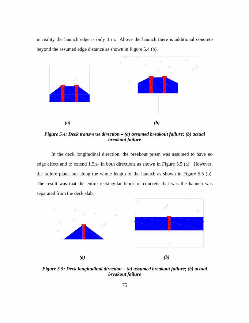
75
in reality the haunch edge is only 3 in. Above the haunch there is additional concrete
beyond the assumed edge distance as shown in Figure 5.4 (b).
(a) (b)
Figure 5.4: Deck transverse direction – (a) assumed breakout failure; (b) actual breakout failure
In the deck longitudinal direction, the breakout prism was assumed to have no
edge effect and to extend 1.5hef in both directions as shown in Figure 5.5 (a). However,
the failure plane ran along the whole length of the haunch as shown in Figure 5.5 (b).
The result was that the entire rectangular block of concrete that was the haunch was
separated from the deck slab.
(a) (b)
Figure 5.5: Deck longitudinal direction – (a) assumed breakout failure; (b) actual breakout failure
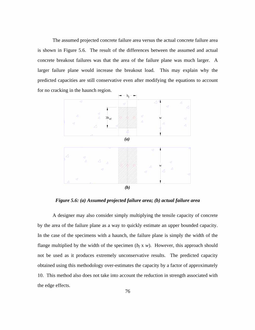
76
The assumed projected concrete failure area versus the actual concrete failure area
is shown in Figure 5.6. The result of the differences between the assumed and actual
concrete breakout failures was that the area of the failure plane was much larger. A
larger failure plane would increase the breakout load. This may explain why the
predicted capacities are still conservative even after modifying the equations to account
for no cracking in the haunch region.
3hef
(a)
(b)
bf
w
w
Figure 5.6: (a) Assumed projected failure area; (b) actual failure area
A designer may also consider simply multiplying the tensile capacity of concrete
by the area of the failure plane as a way to quickly estimate an upper bounded capacity.
In the case of the specimens with a haunch, the failure plane is simply the width of the
flange multiplied by the width of the specimen (bf x w). However, this approach should
not be used as it produces extremely unconservative results. The predicted capacity
obtained using this methodology over-estimates the capacity by a factor of approximately
10. This method also does not take into account the reduction in strength associated with
the edge effects.
77
5.2 EVALUATION OF CURRENT SHEAR CONNECTOR DETAIL
5.2.1 Introduction
The purpose of this experimental program was to determine the effect that a
bridge haunch has on the tensile capacity of a row of shear studs and to use that
information to determine if the current detail will allow for the transfer and redistribution
of the required tensile force during a fracture event. Much has been learned about both
the strength and behavior of the shear studs in specimens with and without a haunch. The
results of this testing program not only demonstrate the effect of the haunch, but they also
can be used to examine the effectiveness of the current standard shear stud bridge detail.
5.2.2 Capacity
The test results clearly show that the bridge haunch reduces the tensile capacity of
the shear studs. The tensile capacity of a row of three studs without a haunch is reduced
by 33% when a 3-in. haunch is in place, and the tensile capacity of a row of two studs
without a haunch is reduced by 22% when a 3-in. haunch is in place.
5.2.3 Ductility
More significant than the decrease in capacity, the tests have also demonstrated
that the specimens with a 3-in. haunch exhibit no ductility at failure. This lack of
ductility is due to the fact that the haunch is not reinforced and that the studs do not
penetrate far enough into the deck to engage the steel reinforcement. The breakout
failure is a tension failure of the concrete, and therefore is a brittle failure. This is a
major problem because it may make the distribution of the tensile force along the length
of the girder impossible during a fracture event. In order to redistribute forces, a system
must have ductility, and this current detail offers no ductility. Figure 5.7 shows the total
separation of the studs and the haunch concrete from the deck. Notice in Figure 5.7 (b)
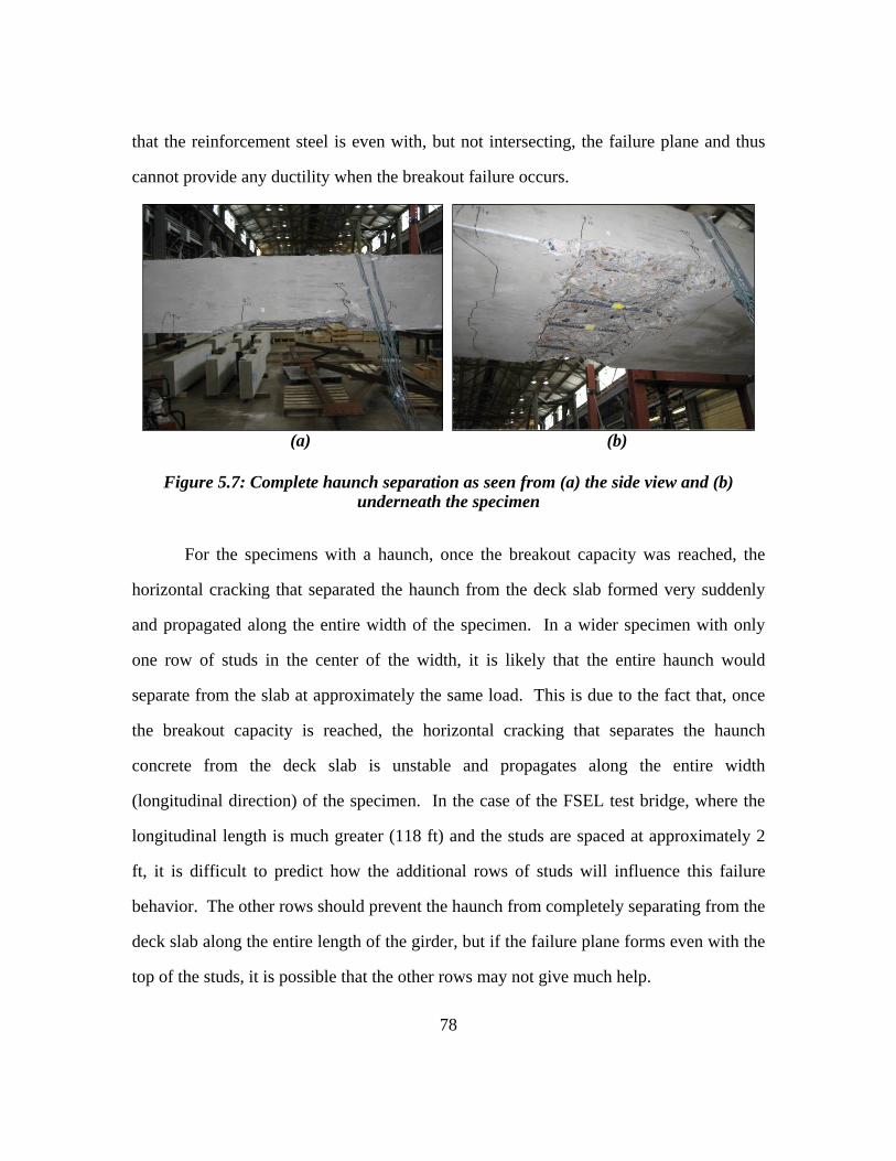
78
that the reinforcement steel is even with, but not intersecting, the failure plane and thus
cannot provide any ductility when the breakout failure occurs.
(a) (b)
Figure 5.7: Complete haunch separation as seen from (a) the side view and (b) underneath the specimen
For the specimens with a haunch, once the breakout capacity was reached, the
horizontal cracking that separated the haunch from the deck slab formed very suddenly
and propagated along the entire width of the specimen. In a wider specimen with only
one row of studs in the center of the width, it is likely that the entire haunch would
separate from the slab at approximately the same load. This is due to the fact that, once
the breakout capacity is reached, the horizontal cracking that separates the haunch
concrete from the deck slab is unstable and propagates along the entire width
(longitudinal direction) of the specimen. In the case of the FSEL test bridge, where the
longitudinal length is much greater (118 ft) and the studs are spaced at approximately 2
ft, it is difficult to predict how the additional rows of studs will influence this failure
behavior. The other rows should prevent the haunch from completely separating from the
deck slab along the entire length of the girder, but if the failure plane forms even with the
top of the studs, it is possible that the other rows may not give much help.
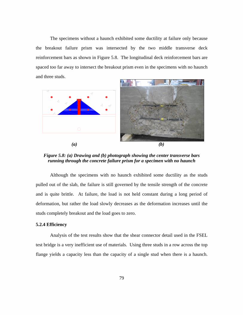
79
The specimens without a haunch exhibited some ductility at failure only because
the breakout failure prism was intersected by the two middle transverse deck
reinforcement bars as shown in Figure 5.8. The longitudinal deck reinforcement bars are
spaced too far away to intersect the breakout prism even in the specimens with no haunch
and three studs.
(a) (b)
Figure 5.8: (a) Drawing and (b) photograph showing the center transverse bars running through the concrete failure prism for a specimen with no haunch
Although the specimens with no haunch exhibited some ductility as the studs
pulled out of the slab, the failure is still governed by the tensile strength of the concrete
and is quite brittle. At failure, the load is not held constant during a long period of
deformation, but rather the load slowly decreases as the deformation increases until the
studs completely breakout and the load goes to zero.
5.2.4 Efficiency
Analysis of the test results show that the shear connector detail used in the FSEL
test bridge is a very inefficient use of materials. Using three studs in a row across the top
flange yields a capacity less than the capacity of a single stud when there is a haunch.
80
Even if there were no haunch, three studs spaced very close together across the top flange
only increases the capacity by approximately 25% when compared to a single stud.
The data from the strain gage data also show that the center stud resists the
majority of the tensile force and that each of the outer studs resists only about 25% of the
total load. Furthermore, in the case with a 3-in. haunch and a row of three studs, at
failure the largest stress in the center stud was approximately 25% of the yield stress, and
the largest stress in the outer studs was approximately 14% of the yield stress. In the
specimens with only one stud and a 3-in. haunch, the single stud experienced a stress
approximately 72% of the yield stress at failure. These results show that grouping the
studs is not an efficient use of materials.
If the studs must be grouped into rows, using two studs in a row is more efficient
than using three studs in a row. When two studs are used in a specimen with a haunch,
the reduction in capacity is not as great as when three studs are used. In addition the
force is evenly distributed between the two studs, and the stress in the studs is higher at
the time of the concrete breakout failure.
5.2.5 Summary
The current detail of using a bridge haunch and grouping the studs in rows of two
or three does not perform well under tensile loading. The haunch greatly reduces the
capacity when multiple studs are used in a row and also prevents the connection from
failing in a ductile manner. Following the current AASHTO and TxDOT standards,
which require the studs to penetrate a minimum of 2 in. into the deck slab, does not allow
the breakout failure prism to engage the deck reinforcement. This creates an extremely
brittle failure and may prevent the redistribution of the tensile forces along the length of
the girder during a fracture event.
81
5.3 POSSIBLE TECHNIQUES TO IMPROVE SHEAR CONNECTOR DETAIL
5.3.1 General Comments
The suggestions in the following sections are possible methods that can be used to
improve the tensile behavior of the current shear stud detail. These suggestions are based
on the assumption that the haunch is a necessary part of bridge construction, which
cannot be eliminated despite the negative effects it has on the tensile behavior of the
studs.
The AASHTO Specifications require that a designer calculate the shear capacity
of a single stud and provide enough studs to resist the required design shear force.
Therefore, as long as the following suggestions do not reduce the number of studs on a
girder or reduce the shear capacity of a single stud then the shear resistance should not
change.
5.3.2 Haunch Reinforcement
A simple way to improve the current detail without changing the spacing or
grouping of the studs is simply to include reinforcement in the haunch area near each row
of studs. Figure 5.9 demonstrates a potential detail for reinforcing the haunch region.
The bar shown in green would be placed on each side of a row of studs. The bar would
need to be spaced close enough to the studs so that it would intersect the breakout failure
plane. The central transverse deck reinforcement bars, which intersected the failure
prism in the specimens with no haunch, were offset from the row of studs by 3 in.
Therefore, this would be an acceptable spacing to offset the proposed haunch
reinforcement bars. The bar would also need to be long enough to develop both ends in
the deck slab. The longitudinal deck reinforcing bars are not shown in this figure.
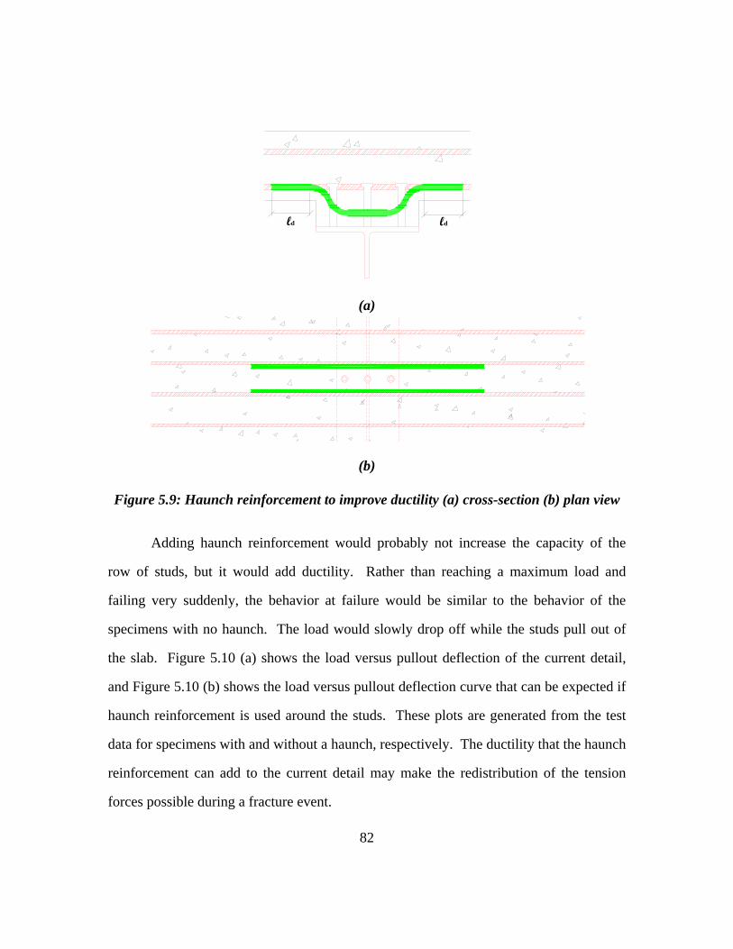
82
ld ld
(a)
(b)
Figure 5.9: Haunch reinforcement to improve ductility (a) cross-section (b) plan view
Adding haunch reinforcement would probably not increase the capacity of the
row of studs, but it would add ductility. Rather than reaching a maximum load and
failing very suddenly, the behavior at failure would be similar to the behavior of the
specimens with no haunch. The load would slowly drop off while the studs pull out of
the slab. Figure 5.10 (a) shows the load versus pullout deflection of the current detail,
and Figure 5.10 (b) shows the load versus pullout deflection curve that can be expected if
haunch reinforcement is used around the studs. These plots are generated from the test
data for specimens with and without a haunch, respectively. The ductility that the haunch
reinforcement can add to the current detail may make the redistribution of the tension
forces possible during a fracture event.
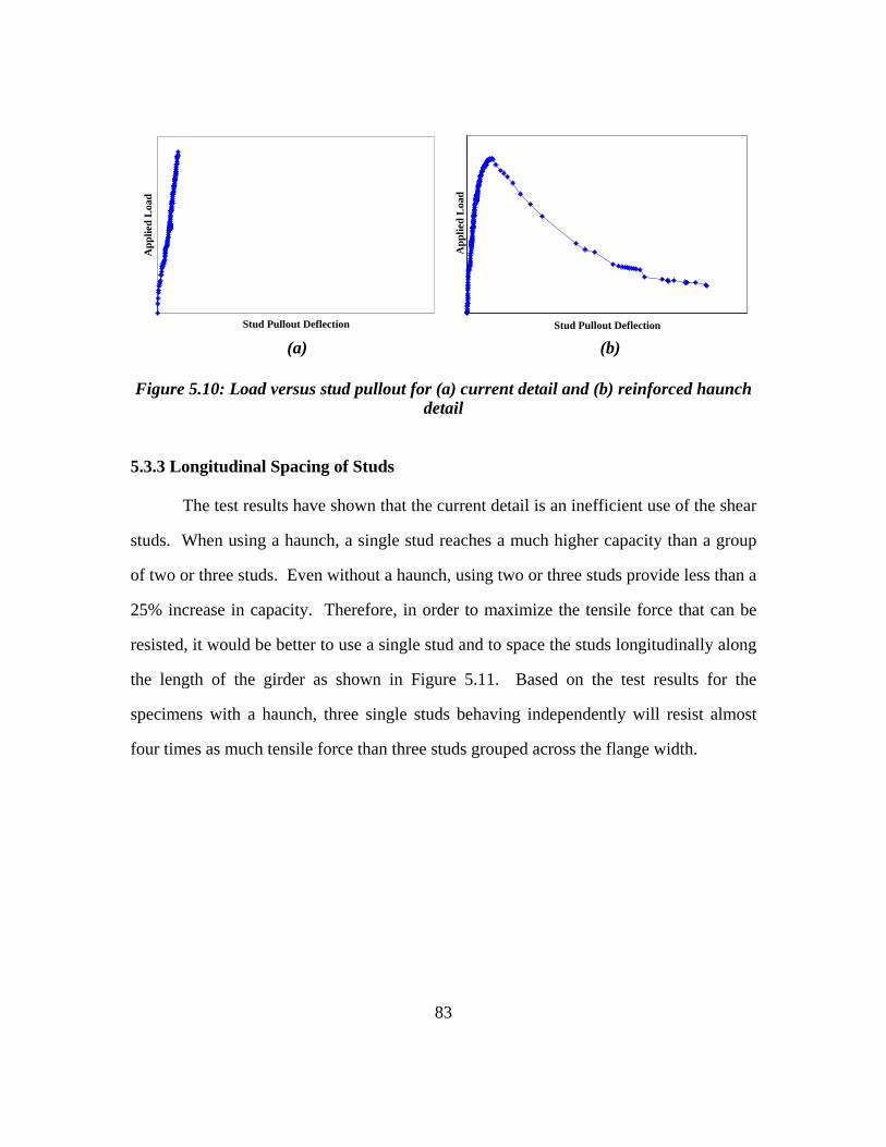
83
0
0
Stud Pullout Deflection
App
lied
Loa
d
0
0
Stud Pullout Deflection
App
lied
Loa
d
(a) (b)
Figure 5.10: Load versus stud pullout for (a) current detail and (b) reinforced haunch detail
5.3.3 Longitudinal Spacing of Studs
The test results have shown that the current detail is an inefficient use of the shear
studs. When using a haunch, a single stud reaches a much higher capacity than a group
of two or three studs. Even without a haunch, using two or three studs provide less than a
25% increase in capacity. Therefore, in order to maximize the tensile force that can be
resisted, it would be better to use a single stud and to space the studs longitudinally along
the length of the girder as shown in Figure 5.11. Based on the test results for the
specimens with a haunch, three single studs behaving independently will resist almost
four times as much tensile force than three studs grouped across the flange width.
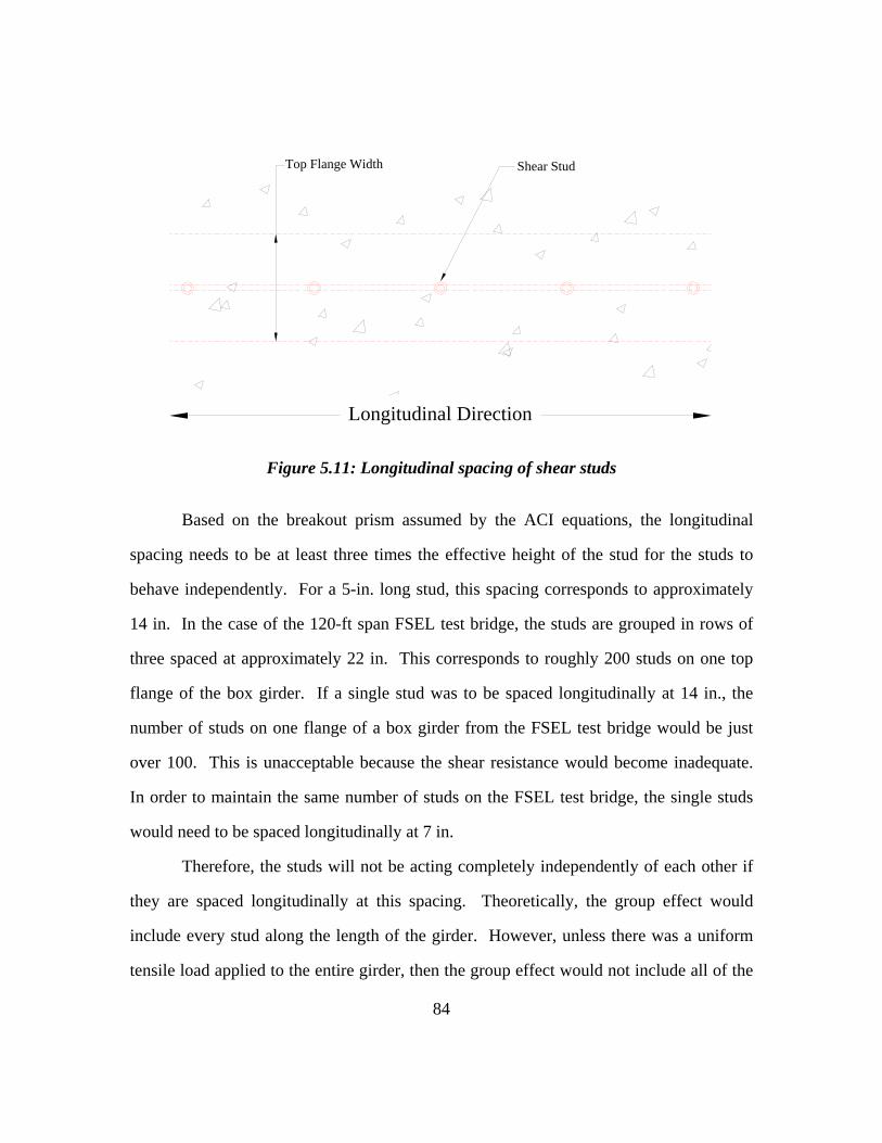
84
Longitudinal Direction
Shear StudTop Flange Width
Figure 5.11: Longitudinal spacing of shear studs
Based on the breakout prism assumed by the ACI equations, the longitudinal
spacing needs to be at least three times the effective height of the stud for the studs to
behave independently. For a 5-in. long stud, this spacing corresponds to approximately
14 in. In the case of the 120-ft span FSEL test bridge, the studs are grouped in rows of
three spaced at approximately 22 in. This corresponds to roughly 200 studs on one top
flange of the box girder. If a single stud was to be spaced longitudinally at 14 in., the
number of studs on one flange of a box girder from the FSEL test bridge would be just
over 100. This is unacceptable because the shear resistance would become inadequate.
In order to maintain the same number of studs on the FSEL test bridge, the single studs
would need to be spaced longitudinally at 7 in.
Therefore, the studs will not be acting completely independently of each other if
they are spaced longitudinally at this spacing. Theoretically, the group effect would
include every stud along the length of the girder. However, unless there was a uniform
tensile load applied to the entire girder, then the group effect would not include all of the
85
studs. During a fracture event the tensile force will initially be applied in the local area
where the crack occurs. Therefore, the group effect will most likely only include the
studs in the vicinity of the fracture.
Even with this group effect, the tensile capacity of three studs spaced
longitudinally will still be much greater than the row of three studs spaced transversely
across the flange width. Three studs grouped transversely across the width of the top
flange experience a very large reduction in capacity because the distance between the
outer studs and the haunch edge is very small. While the single studs spaced
longitudinally may experience a group effect, the edge effect is kept to a minimum
because the stud is in the center of the flange width.
5.3.4 Longer Studs
Another method to improve the current detail is to increase the length of the shear
studs. An increase in the stud length could potentially increase both the tensile capacity
and the ductility of a row of studs. As shown in Equations 5.1 and 5.2, the concrete
breakout load is a function of the effective height raised to the three-halves power. Thus,
for a single stud with no edge or group effects, increasing the length of the stud will
increase the capacity. Using the ACI equations, for a single 7/8-in. diameter stud with no
edge or group effects in Class “S” (4,000 psi) concrete, an increase in the length of the
stud from 5 in. to 7 in. will increase the concrete breakout capacity from 15 kips to 26
kips.
Increasing the stud length will increase the penetration of the studs into the deck
reinforcement mat. Using an 8-in. long stud with a 3-in. haunch would create the same
penetration into the deck reinforcement as the test specimens with 5-in. long studs and no
haunch as shown in Figure 5.12. If the studs extend far enough into the reinforcement
mat, then the breakout failure prism will intersect the deck reinforcement steel. This
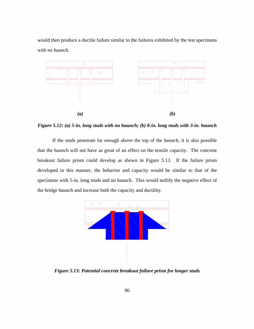
86
would then produce a ductile failure similar to the failures exhibited by the test specimens
with no haunch.
(a) (b)
Figure 5.12: (a) 5-in. long studs with no haunch; (b) 8-in. long studs with 3-in. haunch
If the studs penetrate far enough above the top of the haunch, it is also possible
that the haunch will not have as great of an effect on the tensile capacity. The concrete
breakout failure prism could develop as shown in Figure 5.13. If the failure prism
developed in this manner, the behavior and capacity would be similar to that of the
specimens with 5-in. long studs and no haunch. This would nullify the negative effect of
the bridge haunch and increase both the capacity and ductility.
Figure 5.13: Potential concrete breakout failure prism for longer studs
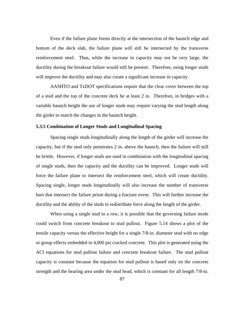
87
Even if the failure plane forms directly at the intersection of the haunch edge and
bottom of the deck slab, the failure plane will still be intersected by the transverse
reinforcement steel. Thus, while the increase in capacity may not be very large, the
ductility during the breakout failure would still be present. Therefore, using longer studs
will improve the ductility and may also create a significant increase in capacity.
AASHTO and TxDOT specifications require that the clear cover between the top
of a stud and the top of the concrete deck be at least 2 in. Therefore, in bridges with a
variable haunch height the use of longer studs may require varying the stud length along
the girder to match the changes in the haunch height.
5.3.5 Combination of Longer Studs and Longitudinal Spacing
Spacing single studs longitudinally along the length of the girder will increase the
capacity, but if the stud only penetrates 2 in. above the haunch, then the failure will still
be brittle. However, if longer studs are used in combination with the longitudinal spacing
of single studs, then the capacity and the ductility can be improved. Longer studs will
force the failure plane to intersect the reinforcement steel, which will create ductility.
Spacing single, longer studs longitudinally will also increase the number of transverse
bars that intersect the failure prism during a fracture event. This will further increase the
ductility and the ability of the studs to redistribute force along the length of the girder.
When using a single stud in a row, it is possible that the governing failure mode
could switch from concrete breakout to stud pullout. Figure 5.14 shows a plot of the
tensile capacity versus the effective height for a single 7/8-in. diameter stud with no edge
or group effects embedded in 4,000 psi cracked concrete. This plot is generated using the
ACI equations for stud pullout failure and concrete breakout failure. The stud pullout
capacity is constant because the equation for stud pullout is based only on the concrete
strength and the bearing area under the stud head, which is constant for all length 7/8-in.
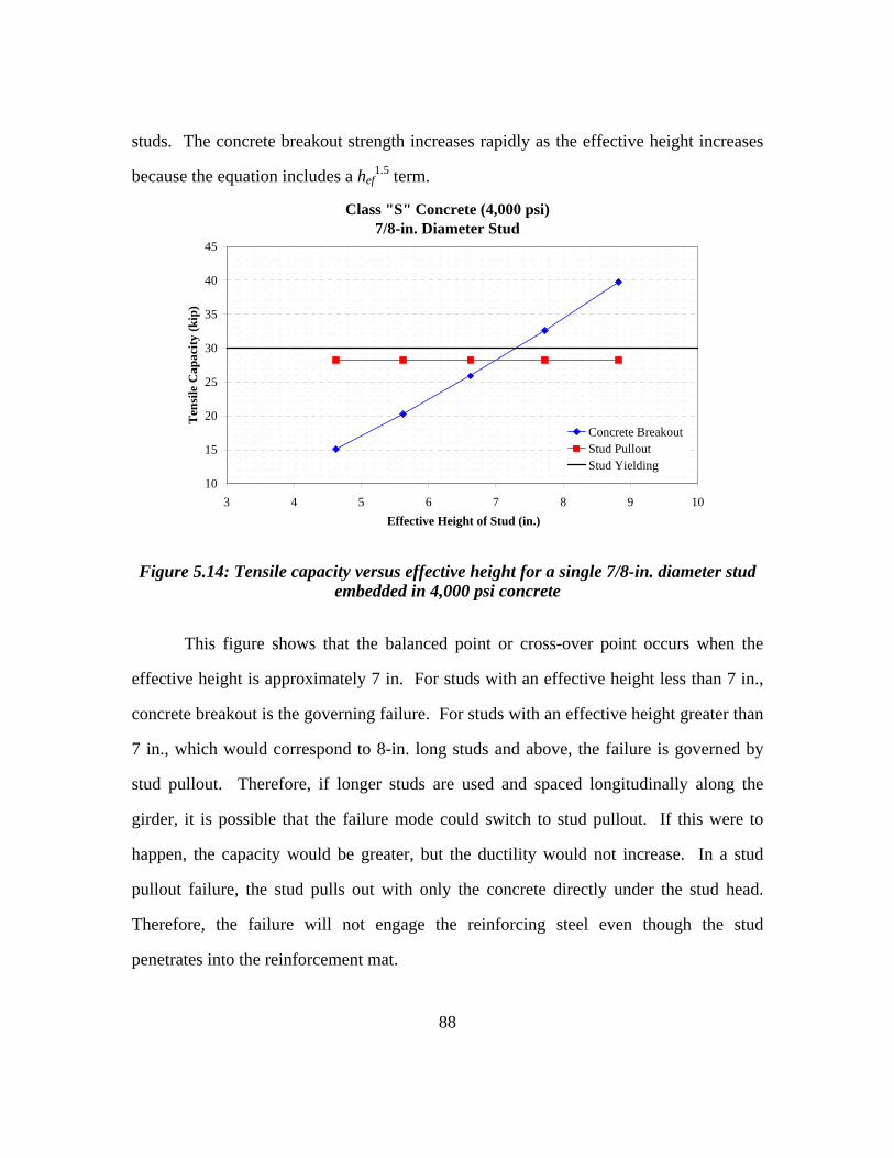
88
studs. The concrete breakout strength increases rapidly as the effective height increases
because the equation includes a hef1.5 term.
Class "S" Concrete (4,000 psi)7/8-in. Diameter Stud
10
15
20
25
30
35
40
45
3 4 5 6 7 8 9 10Effective Height of Stud (in.)
Ten
sile
Cap
acity
(kip
)
Concrete BreakoutStud PulloutStud Yielding
Figure 5.14: Tensile capacity versus effective height for a single 7/8-in. diameter stud embedded in 4,000 psi concrete
This figure shows that the balanced point or cross-over point occurs when the
effective height is approximately 7 in. For studs with an effective height less than 7 in.,
concrete breakout is the governing failure. For studs with an effective height greater than
7 in., which would correspond to 8-in. long studs and above, the failure is governed by
stud pullout. Therefore, if longer studs are used and spaced longitudinally along the
girder, it is possible that the failure mode could switch to stud pullout. If this were to
happen, the capacity would be greater, but the ductility would not increase. In a stud
pullout failure, the stud pulls out with only the concrete directly under the stud head.
Therefore, the failure will not engage the reinforcing steel even though the stud
penetrates into the reinforcement mat.
89
This figure also shows that stud yielding cannot govern for a 7/8-in. stud
embedded in 4,000 psi cracked concrete. However, the pullout strength and the yield
strength are very close. If the concrete strength is increased, then yielding can occur
before a pullout failure. If this is the case, then as long as the effective height is greater
than the balanced effective height, yielding of the stud will occur before a concrete
failure. The cross-over point for a single 7/8-in. diameter stud with no edge or group
effects in various concrete compressive strengths is shown in Table 5.4. This table shows
that yielding will occur before pullout for concrete strengths greater than or equal to
4,500 psi. Thus, for a single 7/8-in. diameter stud with no edge or group effects, yielding
will govern when the effective height is greater than or equal to the balanced effective
height and the concrete strength is greater than or equal to 4,500 psi. (All values in Table
5.4 assume that the concrete is cracked.)
Table 5.4: Cross-over point for a single 7/8-in. diameter stud with no edge or group effects in various concrete compressive strengths
fc' (psi) hef,bal (in.) Np (kip) Nyield (kip)4000 7.02 28.3 30.14500 7.30 31.8 30.15000 7.57 35.3 30.15500 7.81 38.9 30.16000 8.04 42.4 30.16500 8.26 45.9 30.17000 8.47 49.5 30.1
5.3.6 Reduction of Stud Diameter
The methods mentioned in the previous sections are all governed by the tensile
strength of the concrete deck slab, which is inherently a brittle failure. This failure
becomes only slightly ductile when reinforcement bars intersect the failure surfaces. In
order to guarantee that the shear stud connection will be truly ductile, the failure should
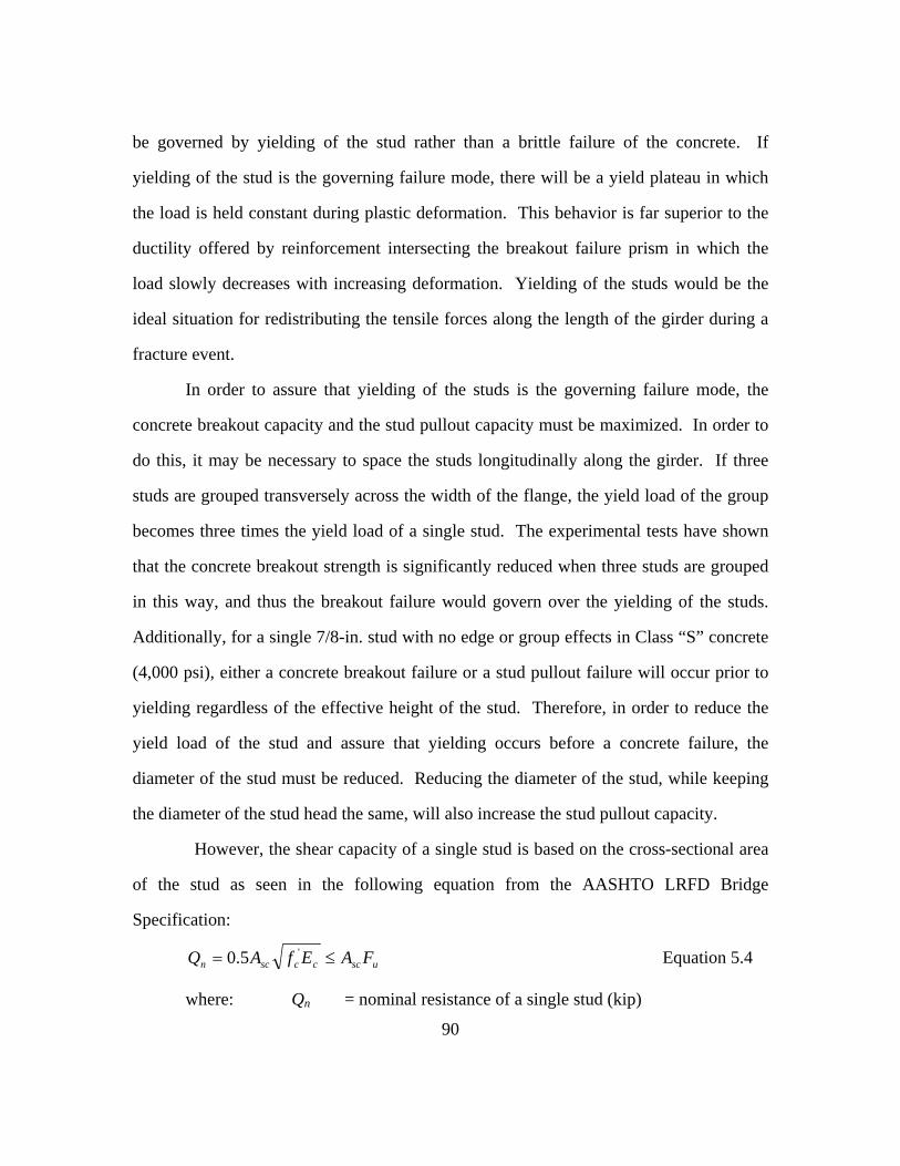
90
be governed by yielding of the stud rather than a brittle failure of the concrete. If
yielding of the stud is the governing failure mode, there will be a yield plateau in which
the load is held constant during plastic deformation. This behavior is far superior to the
ductility offered by reinforcement intersecting the breakout failure prism in which the
load slowly decreases with increasing deformation. Yielding of the studs would be the
ideal situation for redistributing the tensile forces along the length of the girder during a
fracture event.
In order to assure that yielding of the studs is the governing failure mode, the
concrete breakout capacity and the stud pullout capacity must be maximized. In order to
do this, it may be necessary to space the studs longitudinally along the girder. If three
studs are grouped transversely across the width of the flange, the yield load of the group
becomes three times the yield load of a single stud. The experimental tests have shown
that the concrete breakout strength is significantly reduced when three studs are grouped
in this way, and thus the breakout failure would govern over the yielding of the studs.
Additionally, for a single 7/8-in. stud with no edge or group effects in Class “S” concrete
(4,000 psi), either a concrete breakout failure or a stud pullout failure will occur prior to
yielding regardless of the effective height of the stud. Therefore, in order to reduce the
yield load of the stud and assure that yielding occurs before a concrete failure, the
diameter of the stud must be reduced. Reducing the diameter of the stud, while keeping
the diameter of the stud head the same, will also increase the stud pullout capacity.
However, the shear capacity of a single stud is based on the cross-sectional area
of the stud as seen in the following equation from the AASHTO LRFD Bridge
Specification:
uscccscn FAEfAQ ≤= '5.0 Equation 5.4
where: Qn = nominal resistance of a single stud (kip)
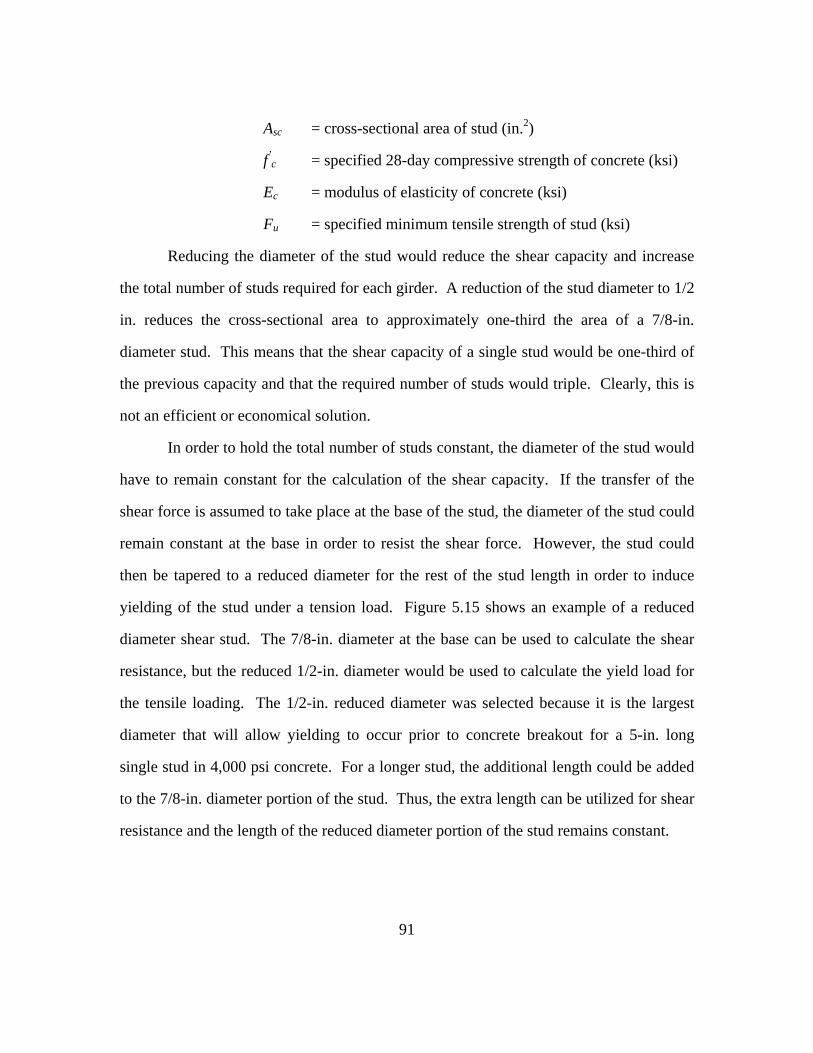
91
Asc = cross-sectional area of stud (in.2)
f’c = specified 28-day compressive strength of concrete (ksi)
Ec = modulus of elasticity of concrete (ksi)
Fu = specified minimum tensile strength of stud (ksi)
Reducing the diameter of the stud would reduce the shear capacity and increase
the total number of studs required for each girder. A reduction of the stud diameter to 1/2
in. reduces the cross-sectional area to approximately one-third the area of a 7/8-in.
diameter stud. This means that the shear capacity of a single stud would be one-third of
the previous capacity and that the required number of studs would triple. Clearly, this is
not an efficient or economical solution.
In order to hold the total number of studs constant, the diameter of the stud would
have to remain constant for the calculation of the shear capacity. If the transfer of the
shear force is assumed to take place at the base of the stud, the diameter of the stud could
remain constant at the base in order to resist the shear force. However, the stud could
then be tapered to a reduced diameter for the rest of the stud length in order to induce
yielding of the stud under a tension load. Figure 5.15 shows an example of a reduced
diameter shear stud. The 7/8-in. diameter at the base can be used to calculate the shear
resistance, but the reduced 1/2-in. diameter would be used to calculate the yield load for
the tensile loading. The 1/2-in. reduced diameter was selected because it is the largest
diameter that will allow yielding to occur prior to concrete breakout for a 5-in. long
single stud in 4,000 psi concrete. For a longer stud, the additional length could be added
to the 7/8-in. diameter portion of the stud. Thus, the extra length can be utilized for shear
resistance and the length of the reduced diameter portion of the stud remains constant.
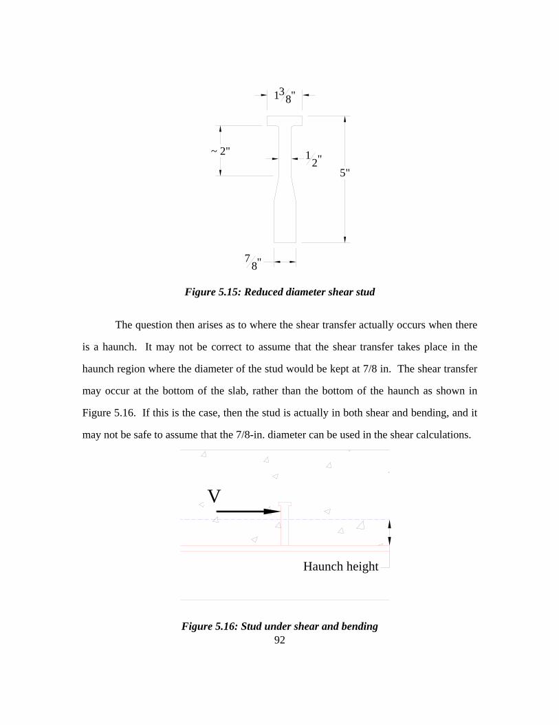
92
78"
5"
138"
12"
~ 2"
Figure 5.15: Reduced diameter shear stud
The question then arises as to where the shear transfer actually occurs when there
is a haunch. It may not be correct to assume that the shear transfer takes place in the
haunch region where the diameter of the stud would be kept at 7/8 in. The shear transfer
may occur at the bottom of the slab, rather than the bottom of the haunch as shown in
Figure 5.16. If this is the case, then the stud is actually in both shear and bending, and it
may not be safe to assume that the 7/8-in. diameter can be used in the shear calculations.
Haunch height
V
Figure 5.16: Stud under shear and bending
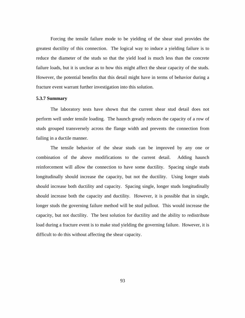
93
Forcing the tensile failure mode to be yielding of the shear stud provides the
greatest ductility of this connection. The logical way to induce a yielding failure is to
reduce the diameter of the studs so that the yield load is much less than the concrete
failure loads, but it is unclear as to how this might affect the shear capacity of the studs.
However, the potential benefits that this detail might have in terms of behavior during a
fracture event warrant further investigation into this solution.
5.3.7 Summary
The laboratory tests have shown that the current shear stud detail does not
perform well under tensile loading. The haunch greatly reduces the capacity of a row of
studs grouped transversely across the flange width and prevents the connection from
failing in a ductile manner.
The tensile behavior of the shear studs can be improved by any one or
combination of the above modifications to the current detail. Adding haunch
reinforcement will allow the connection to have some ductility. Spacing single studs
longitudinally should increase the capacity, but not the ductility. Using longer studs
should increase both ductility and capacity. Spacing single, longer studs longitudinally
should increase both the capacity and ductility. However, it is possible that in single,
longer studs the governing failure method will be stud pullout. This would increase the
capacity, but not ductility. The best solution for ductility and the ability to redistribute
load during a fracture event is to make stud yielding the governing failure. However, it is
difficult to do this without affecting the shear capacity.
94
CHAPTER 6
Conclusions and Recommendations
6.1 SUMMARY OF OBJECTIVES
In order for a simply supported twin box girder steel bridge to be considered non-
fracture critical, the bridge system must have the ability to transfer the load that was
resisted by the fractured girder over to the other girder. As the fractured girder drops
down, the shear studs will be loaded in tension. If the studs can transfer the tensile force
to the slab, then the slab must have the ability to transfer the force to the other girder.
Finally, the non-fractured girder must have enough reserve capacity to support the entire
bridge dead and live load. An important assumption involved in this load transfer is that
the studs and the slab behave in a ductile manner so that the load can be distributed along
the length of the girder.
When analyzing the tensile capacity of the shear studs, it was determined that the
bridge haunch would likely have a detrimental effect on the tensile capacity of a row of
studs. In order to determine the effect of the haunch, a series of laboratory tests were
performed on bridge deck sections with both no haunch and a 3-in. haunch. The results
of these tests were used to evaluate the current haunch detail and to determine if the studs
could transfer the required tensile force during a fracture event. The results were also
used to develop possible techniques that can be used to improve the detail so that the
studs might perform better during a fracture event.
6.2 CONCLUSIONS
The following conclusions were drawn from the results of the tests performed on
the 12 bridge deck segments:
95
1) The haunch clearly has a detrimental effect on the tensile capacity of
the shear studs. Specimens with multiple studs across the flange width
and a 3-in. haunch failed at significantly lower loads than the
corresponding specimens with no haunch. In specimens with a 3-in.
haunch, adding studs to the row decreases the distance to the haunch
edge and thus decreases the capacity.
2) Following the minimum design provisions, which require the stud to
penetrate 2 in. into the deck slab, will create a brittle failure when the
studs are loaded in tension because this depth of embedment does not
create an adequate penetration above the bottom layer of the
reinforcement steel. The specimens with a 3-in. haunch experienced
no ductility at failure because the deck reinforcement steel did not
intersect the concrete failure plane. Conversely, the specimens
without a haunch experienced some ductility at failure – the load
dropped off slowly as the deformations increased – because the deck
reinforcement intersected the failure plane.
3) Due to the lack of ductility seen in the specimens with a 3-in. haunch,
it may not be possible for the studs to distribute the required tensile
force along the length of the girder during a fracture event. If this
cannot happen, the studs will not be able to transfer the load into the
slab and to the non-fractured girder.
4) Grouping studs transversely across the top flange width is an
inefficient way to distribute the studs along the girder. In specimens
with a 3-in. haunch, this arrangement creates a tensile capacity that is
lower than the capacity of a single stud. Even in specimens with no
96
haunch, the capacity of three studs in a row is only slightly higher than
the capacity of a single stud. The shear stud gage data also show that
studs grouped transversely do not experience large stresses prior to a
concrete breakout failure and that the force is not distributed evenly
among the studs. In specimens with three studs, the center stud resists
approximately half of the total force, while each of the outer studs
resist about one-quarter of the total force.
5) During a fracture event the slab will likely experience significant
cracking. The experimental tests were successful in duplicating this
behavior as all of the deck segments cracked prior to the concrete
breakout failure. While specimens with a 3-in. haunch had flexural
cracks at the haunch edges, the increased depth in the haunch area
prevented flexural cracking from occurring in that area. Flexural
cracking did occur at the mid-span location for all of the specimens
without a haunch.
6) The strain gages on the reinforcement steel show that no yielding of
the deck reinforcement took place in any of the specimens with a 3-in.
haunch. Yielding took place in the specimens without a haunch, but
the deck segments experienced very little plastic deformation. The
load versus slab deflection data also confirms that the deck segments
did not experience much plastic deformation prior to the tensile failure
of the shear stud connection. Typically, for the specimens without a
haunch, the mid-span strain in the bottom bars was just slightly above
the yield strain at maximum load. However, in some of the specimens,
97
strains significantly above the yield strain were measured as the
breakout prism developed and the studs pulled out of the deck.
6.3 RECOMMENDATIONS AND FUTURE WORK
Based on the results of the tests performed on the 12 bridge deck segments, the
following recommendations are suggested to improve the tensile behavior of the shear
stud connection. These suggestions have not yet been tested in the laboratory; therefore,
it is recommended that future laboratory tests are performed to determine the effect of
each method and to optimize the detail accordingly.
1) Without changing the practice of grouping the studs transversely
across the top flange, the simplest way to improve the behavior of the
studs is to add haunch reinforcement around each row of studs. This
will improve the ductility of the studs and help with the redistribution
of force along the length of the girder during a fracture event.
2) Rather than grouping studs transversely in rows spaced far apart, use
one stud in the center of the flange and space these single studs
longitudinally at a distance that will allow for the same shear
resistance. This will increase the tensile capacity so that less of the
total span length would be required to resist the tension force during a
fracture event.
3) Another method to improve the shear stud detail is to increase the
length of the studs. Increasing the length of the shear studs, while
keeping the haunch height constant, will increase the penetration of the
studs into the deck reinforcement mat. This will force the breakout
failure plane to cross the reinforcement, which will increase the
ductility. Increasing the ductility will help with the redistribution of
98
force along the length of the girder during a fracture event. It is
possible that using longer studs will also reduce the effect that the
haunch has on the capacity.
4) If longer studs are used in combination with the longitudinal spacing
of single studs, then the capacity and the ductility can be improved.
Future tests need to be done to verify that stud pullout will not govern
over concrete breakout. A stud pullout failure would increase the
capacity of the current detail, but it would not improve ductility.
5) The best way to improve the tensile behavior of the shear stud detail is
to guarantee that yielding of the shear studs is the governing failure
mode. This will allow for the greatest ductility and redistribution of
load. A possible technique to ensure yielding of the stud is to reduce
the diameter of the stud in order for yielding of the reduced section to
control the tensile capacity, but to keep the base diameter constant for
shear resistance. Future work is needed to develop a detail that will
allow for yielding of the stud to govern in tension, but that will not
reduce the shear capacity of the studs.
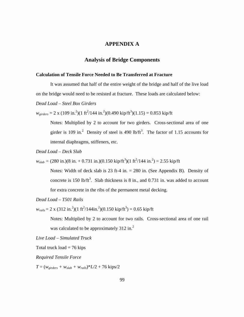
99
APPENDIX A
Analysis of Bridge Components
Calculation of Tensile Force Needed to Be Transferred at Fracture
It was assumed that half of the entire weight of the bridge and half of the live load
on the bridge would need to be resisted at fracture. These loads are calculated below:
Dead Load – Steel Box Girders
wgirders = 2 x (109 in.2)(1 ft2/144 in.2)(0.490 kip/ft3)(1.15) = 0.853 kip/ft
Notes: Multiplied by 2 to account for two girders. Cross-sectional area of one
girder is 109 in.2 Density of steel is 490 lb/ft3. The factor of 1.15 accounts for
internal diaphragms, stiffeners, etc.
Dead Load – Deck Slab
wslab = (280 in.)(8 in. + 0.731 in.)(0.150 kip/ft3)(1 ft2/144 in.2) = 2.55 kip/ft
Notes: Width of deck slab is 23 ft-4 in. = 280 in. (See Appendix B). Density of
concrete is 150 lb/ft3. Slab thickness is 8 in., and 0.731 in. was added to account
for extra concrete in the ribs of the permanent metal decking.
Dead Load – T501 Rails
wrails = 2 x (312 in.2)(1 ft2/144in.2)(0.150 kip/ft3) = 0.65 kip/ft
Notes: Multiplied by 2 to account for two rails. Cross-sectional area of one rail
was calculated to be approximately 312 in.2
Live Load – Simulated Truck
Total truck load = 76 kips
Required Tensile Force
T = (wgirders + wslab + wrails)*L/2 + 76 kips/2
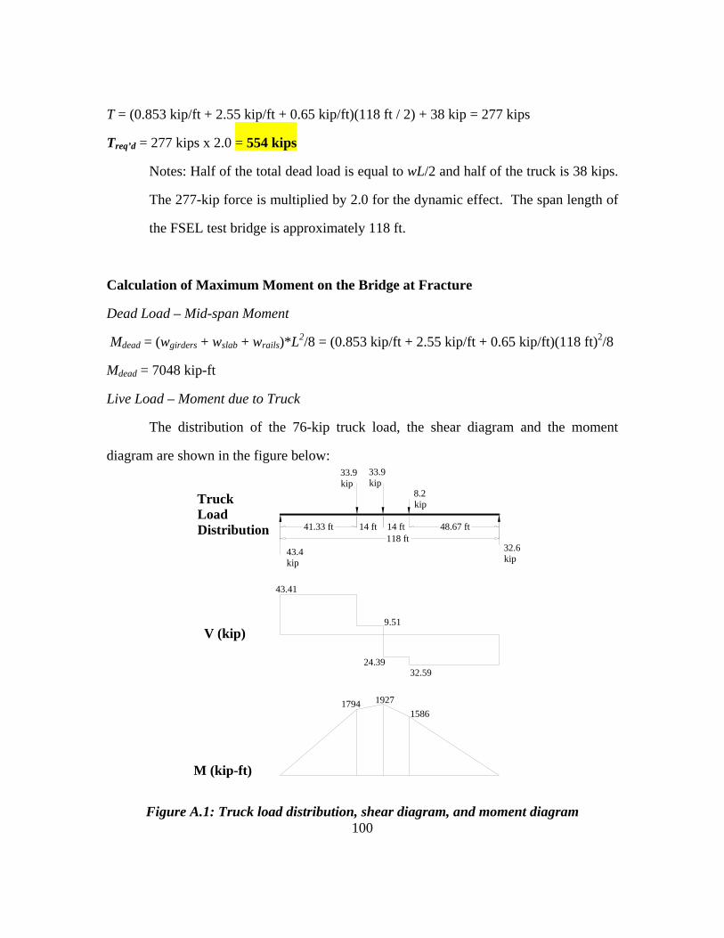
100
T = (0.853 kip/ft + 2.55 kip/ft + 0.65 kip/ft)(118 ft / 2) + 38 kip = 277 kips
Treq’d = 277 kips x 2.0 = 554 kips
Notes: Half of the total dead load is equal to wL/2 and half of the truck is 38 kips.
The 277-kip force is multiplied by 2.0 for the dynamic effect. The span length of
the FSEL test bridge is approximately 118 ft.
Calculation of Maximum Moment on the Bridge at Fracture
Dead Load – Mid-span Moment
Mdead = (wgirders + wslab + wrails)*L2/8 = (0.853 kip/ft + 2.55 kip/ft + 0.65 kip/ft)(118 ft)2/8
Mdead = 7048 kip-ft
Live Load – Moment due to Truck
The distribution of the 76-kip truck load, the shear diagram and the moment
diagram are shown in the figure below:
43.4 kip
32.6 kip
8.2 kip
33.9 kip
33.9 kip
41.33 ft 14 ft 14 ft 48.67 ft118 ft
V (kip)
43.41
9.51
24.3932.59
1794 19271586
M (kip-ft)
Truck Load Distribution
Figure A.1: Truck load distribution, shear diagram, and moment diagram
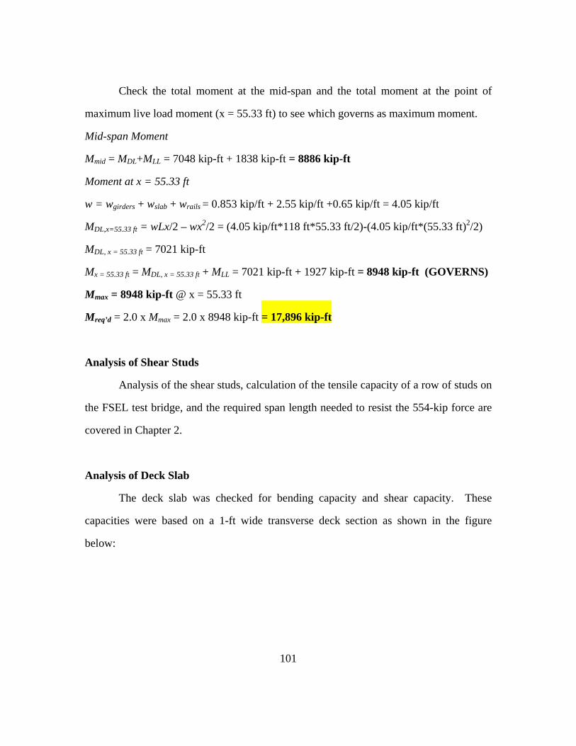
101
Check the total moment at the mid-span and the total moment at the point of
maximum live load moment (x = 55.33 ft) to see which governs as maximum moment.
Mid-span Moment
Mmid = MDL+MLL = 7048 kip-ft + 1838 kip-ft = 8886 kip-ft
Moment at x = 55.33 ft
w = wgirders + wslab + wrails = 0.853 kip/ft + 2.55 kip/ft +0.65 kip/ft = 4.05 kip/ft
MDL,x=55.33 ft = wLx/2 – wx2/2 = (4.05 kip/ft*118 ft*55.33 ft/2)-(4.05 kip/ft*(55.33 ft)2/2)
MDL, x = 55.33 ft = 7021 kip-ft
Mx = 55.33 ft = MDL, x = 55.33 ft + MLL = 7021 kip-ft + 1927 kip-ft = 8948 kip-ft (GOVERNS)
Mmax = 8948 kip-ft @ x = 55.33 ft
Mreq’d = 2.0 x Mmax = 2.0 x 8948 kip-ft = 17,896 kip-ft
Analysis of Shear Studs
Analysis of the shear studs, calculation of the tensile capacity of a row of studs on
the FSEL test bridge, and the required span length needed to resist the 554-kip force are
covered in Chapter 2.
Analysis of Deck Slab
The deck slab was checked for bending capacity and shear capacity. These
capacities were based on a 1-ft wide transverse deck section as shown in the figure
below:
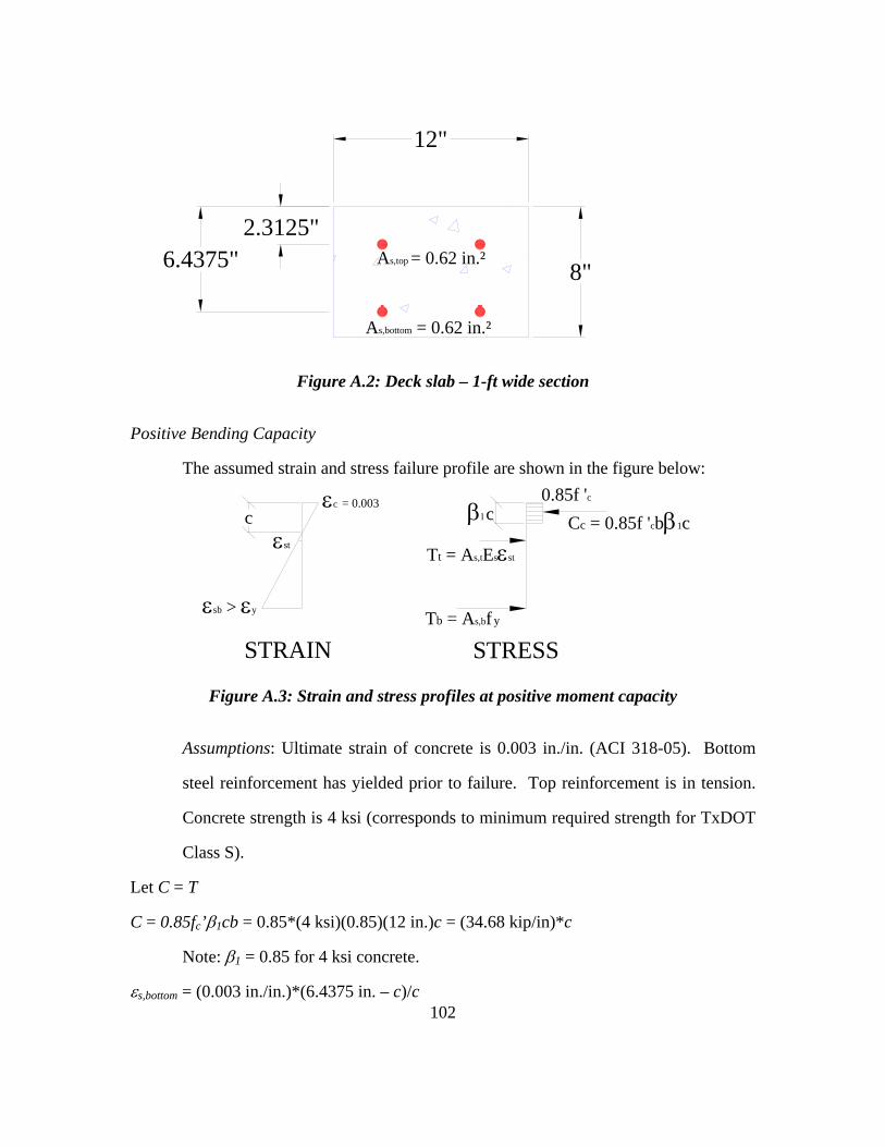
102
8"
12"
2.3125"6.4375"
As,bottom = 0.62 in.²
As,top = 0.62 in.²
Figure A.2: Deck slab – 1-ft wide section
Positive Bending Capacity
The assumed strain and stress failure profile are shown in the figure below:
εsb > εy
εst
εc = 0.003 c
Tb = As,bf y
Tt = As,tEsεst
0.85f 'c Cc = 0.85f 'cbβ1c
STRAIN STRESS
β1c
Figure A.3: Strain and stress profiles at positive moment capacity
Assumptions: Ultimate strain of concrete is 0.003 in./in. (ACI 318-05). Bottom
steel reinforcement has yielded prior to failure. Top reinforcement is in tension.
Concrete strength is 4 ksi (corresponds to minimum required strength for TxDOT
Class S).
Let C = T
C = 0.85fc’β1cb = 0.85*(4 ksi)(0.85)(12 in.)c = (34.68 kip/in)*c
Note: β1 = 0.85 for 4 ksi concrete.
εs,bottom = (0.003 in./in.)*(6.4375 in. – c)/c
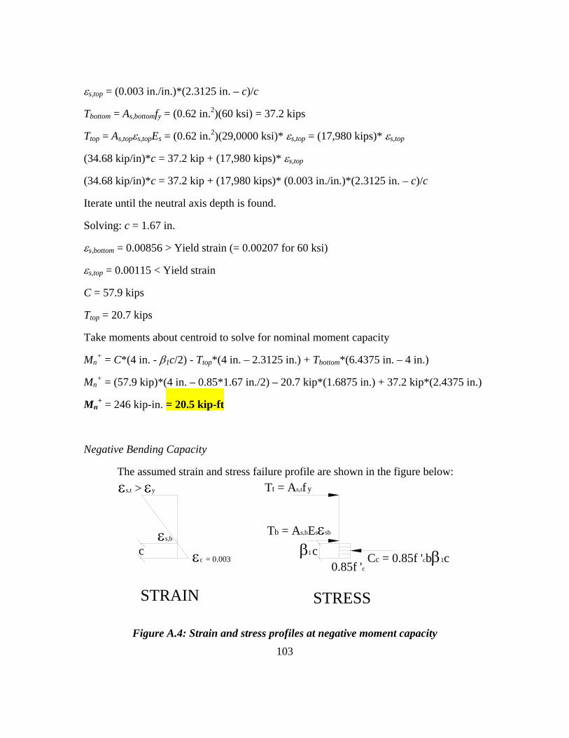
103
εs,top = (0.003 in./in.)*(2.3125 in. – c)/c
Tbottom = As,bottomfy = (0.62 in.2)(60 ksi) = 37.2 kips
Ttop = As,topεs,topEs = (0.62 in.2)(29,0000 ksi)* εs,top = (17,980 kips)* εs,top
(34.68 kip/in)*c = 37.2 kip + (17,980 kips)* εs,top
(34.68 kip/in)*c = 37.2 kip + (17,980 kips)* (0.003 in./in.)*(2.3125 in. – c)/c
Iterate until the neutral axis depth is found.
Solving: c = 1.67 in.
εs,bottom = 0.00856 > Yield strain (= 0.00207 for 60 ksi)
εs,top = 0.00115 < Yield strain
C = 57.9 kips
Ttop = 20.7 kips
Take moments about centroid to solve for nominal moment capacity
Mn+ = C*(4 in. - β1c/2) - Ttop*(4 in. – 2.3125 in.) + Tbottom*(6.4375 in. – 4 in.)
Mn+ = (57.9 kip)*(4 in. – 0.85*1.67 in./2) – 20.7 kip*(1.6875 in.) + 37.2 kip*(2.4375 in.)
Mn+ = 246 kip-in. = 20.5 kip-ft
Negative Bending Capacity
The assumed strain and stress failure profile are shown in the figure below:
STRAIN STRESS
εc = 0.003
εs,t > εy
εs,b
0.85f 'c Cc = 0.85f 'cbβ1cβ1c
Tb = As,bEsεsb
Tt = As,tf y
c
Figure A.4: Strain and stress profiles at negative moment capacity
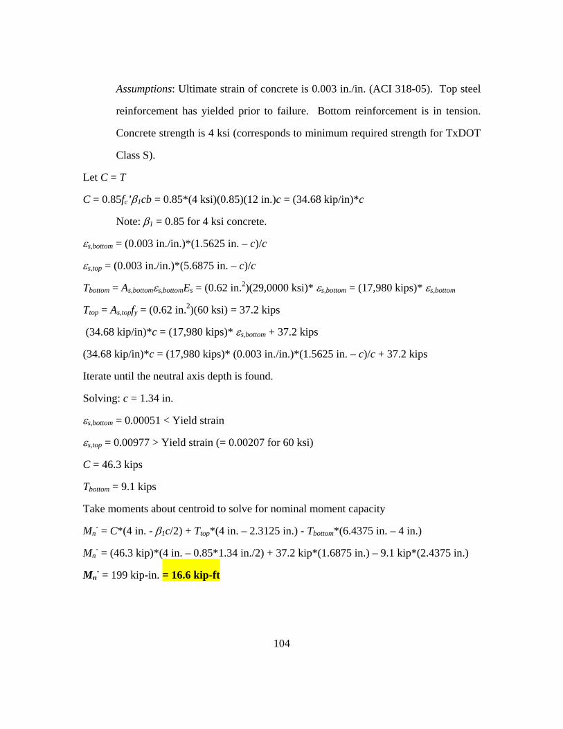
104
Assumptions: Ultimate strain of concrete is 0.003 in./in. (ACI 318-05). Top steel
reinforcement has yielded prior to failure. Bottom reinforcement is in tension.
Concrete strength is 4 ksi (corresponds to minimum required strength for TxDOT
Class S).
Let C = T
C = 0.85fc’β1cb = 0.85*(4 ksi)(0.85)(12 in.)c = (34.68 kip/in)*c
Note: β1 = 0.85 for 4 ksi concrete.
εs,bottom = (0.003 in./in.)*(1.5625 in. – c)/c
εs,top = (0.003 in./in.)*(5.6875 in. – c)/c
Tbottom = As,bottomεs,bottomEs = (0.62 in.2)(29,0000 ksi)* εs,bottom = (17,980 kips)* εs,bottom
Ttop = As,topfy = (0.62 in.2)(60 ksi) = 37.2 kips
(34.68 kip/in)*c = (17,980 kips)* εs,bottom + 37.2 kips
(34.68 kip/in)*c = (17,980 kips)* (0.003 in./in.)*(1.5625 in. – c)/c + 37.2 kips
Iterate until the neutral axis depth is found.
Solving: c = 1.34 in.
εs,bottom = 0.00051 < Yield strain
εs,top = 0.00977 > Yield strain (= 0.00207 for 60 ksi)
C = 46.3 kips
Tbottom = 9.1 kips
Take moments about centroid to solve for nominal moment capacity
Mn- = C*(4 in. - β1c/2) + Ttop*(4 in. – 2.3125 in.) - Tbottom*(6.4375 in. – 4 in.)
Mn- = (46.3 kip)*(4 in. – 0.85*1.34 in./2) + 37.2 kip*(1.6875 in.) – 9.1 kip*(2.4375 in.)
Mn- = 199 kip-in. = 16.6 kip-ft
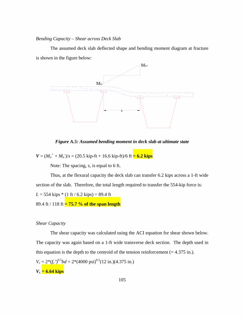
105
Bending Capacity – Shear across Deck Slab
The assumed deck slab deflected shape and bending moment diagram at fracture
is shown in the figure below: Mn+
Mn-
s
Figure A.5: Assumed bending moment in deck slab at ultimate state
V = (Mn+ + Mn
-)/s = (20.5 kip-ft + 16.6 kip-ft)/6 ft = 6.2 kips
Note: The spacing, s, is equal to 6 ft.
Thus, at the flexural capacity the deck slab can transfer 6.2 kips across a 1-ft wide
section of the slab. Therefore, the total length required to transfer the 554-kip force is:
L = 554 kips * (1 ft / 6.2 kips) = 89.4 ft
89.4 ft / 118 ft = 75.7 % of the span length
Shear Capacity
The shear capacity was calculated using the ACI equation for shear shown below.
The capacity was again based on a 1-ft wide transverse deck section. The depth used in
this equation is the depth to the centroid of the tension reinforcement (= 4.375 in.).
Vc = 2*(fc’)0.5bd = 2*(4000 psi)0.5(12 in.)(4.375 in.)
Vc = 6.64 kips
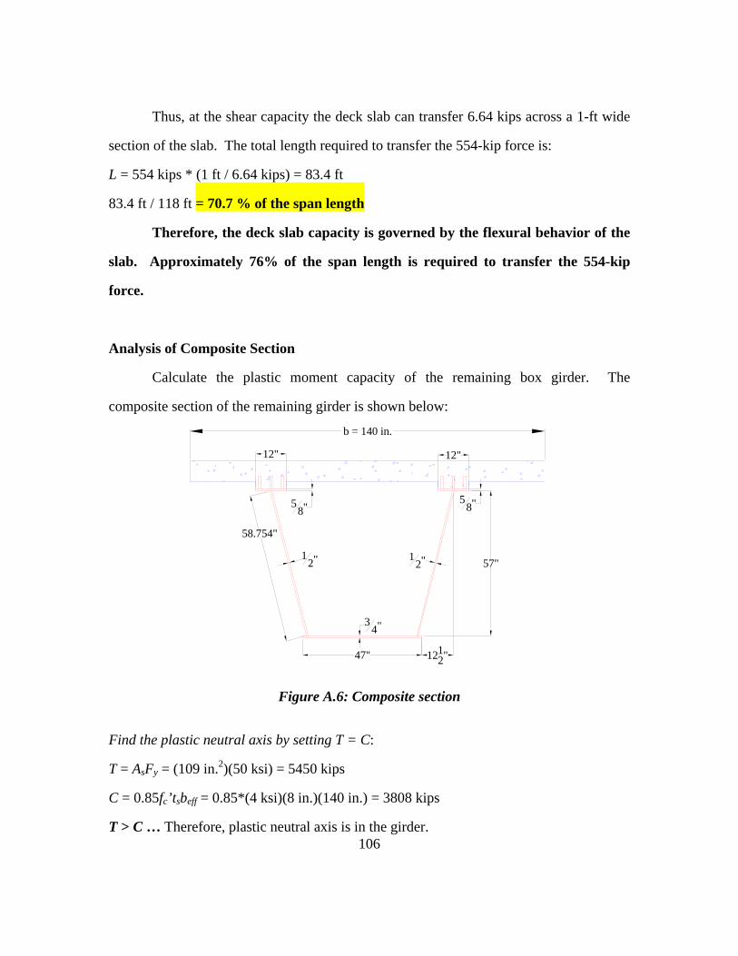
106
Thus, at the shear capacity the deck slab can transfer 6.64 kips across a 1-ft wide
section of the slab. The total length required to transfer the 554-kip force is:
L = 554 kips * (1 ft / 6.64 kips) = 83.4 ft
83.4 ft / 118 ft = 70.7 % of the span length
Therefore, the deck slab capacity is governed by the flexural behavior of the
slab. Approximately 76% of the span length is required to transfer the 554-kip
force.
Analysis of Composite Section
Calculate the plastic moment capacity of the remaining box girder. The
composite section of the remaining girder is shown below:
b = 140 in.
12" 12"
58"5
8"
47"
58.754"
12"1
2"
34"
1212"
57"
Figure A.6: Composite section
Find the plastic neutral axis by setting T = C:
T = AsFy = (109 in.2)(50 ksi) = 5450 kips
C = 0.85fc’tsbeff = 0.85*(4 ksi)(8 in.)(140 in.) = 3808 kips
T > C … Therefore, plastic neutral axis is in the girder.
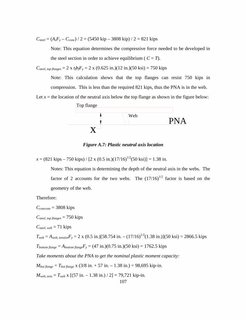
107
Csteel = (AsFy – Cconc) / 2 = (5450 kip – 3808 kip) / 2 = 821 kips
Note: This equation determines the compressive force needed to be developed in
the steel section in order to achieve equilibrium ( C = T).
Csteel, top flanges = 2 x tfbfFy = 2 x (0.625 in.)(12 in.)(50 ksi) = 750 kips
Note: This calculation shows that the top flanges can resist 750 kips in
compression. This is less than the required 821 kips, thus the PNA is in the web.
Let x = the location of the neutral axis below the top flange as shown in the figure below:
PNAx
Top flange
Web
Figure A.7: Plastic neutral axis location
x = (821 kips – 750 kips) / [2 x (0.5 in.)(17/16)1/2(50 ksi)] = 1.38 in.
Notes: This equation is determining the depth of the neutral axis in the webs. The
factor of 2 accounts for the two webs. The (17/16)1/2 factor is based on the
geometry of the web.
Therefore:
Cconcrete = 3808 kips
Csteel, top flanges = 750 kips
Csteel, web = 71 kips
Tweb = Aweb, tensionFy = 2 x (0.5 in.)[58.754 in. – (17/16)1/2(1.38 in.)](50 ksi) = 2866.5 kips
Tbottom flange = Abottom flangeFy = (47 in.)(0.75 in.)(50 ksi) = 1762.5 kips
Take moments about the PNA to get the nominal plastic moment capacity:
Mbot flange = Tbot flange x (3/8 in. + 57 in. – 1.38 in.) = 98,695 kip-in.
Mweb, tens = Tweb x [(57 in. – 1.38 in.) / 2] = 79,721 kip-in.
108
Mweb,comp = Csteel,web x (1.38 in. / 2) = 49 kip-in.
Mtop flange = Cstee;, top flanges x (5/16 in. + 1.38 in.) = 1,268 kip-in.
Mconcrete = Cconc x (4 in. + 3 in. + 5/8 in. + 1.38 in.) = 34,282 kip-in.
Note: The 3-in. term added in the moment arm accounts for the haunch which
puts the deck slab 3 in. above the top of the steel girder.
Thus, Mp = 98,695 kip-in. + 79,721 kip-in. + 49 kip-in. + 1,268 kip-in. + 34,282 kip-in.
Mp = 214,015 kip-in. = 17,835 kip-ft
Recall that Mmax = 17,896 kip-ft (with the amplification factor of 2.0 for
dynamic effect). The plastic moment capacity appears to have just enough capacity
to resist the required moment at fracture.
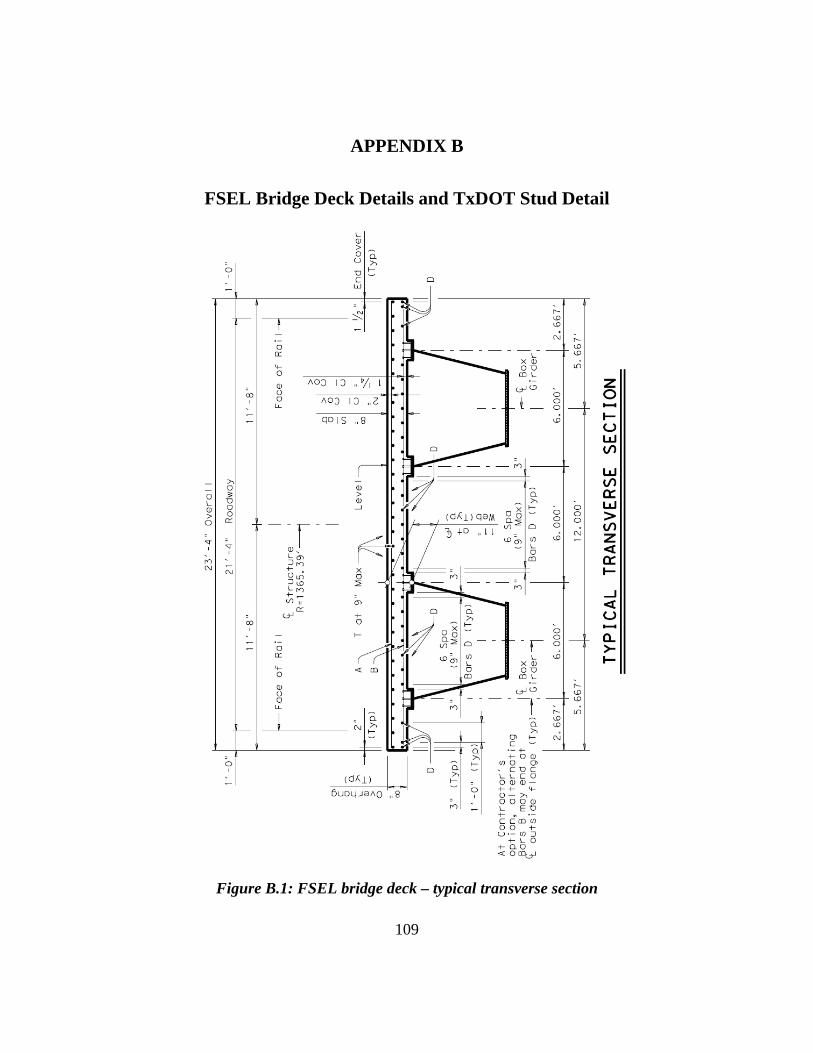
109
APPENDIX B
FSEL Bridge Deck Details and TxDOT Stud Detail
Figure B.1: FSEL bridge deck – typical transverse section
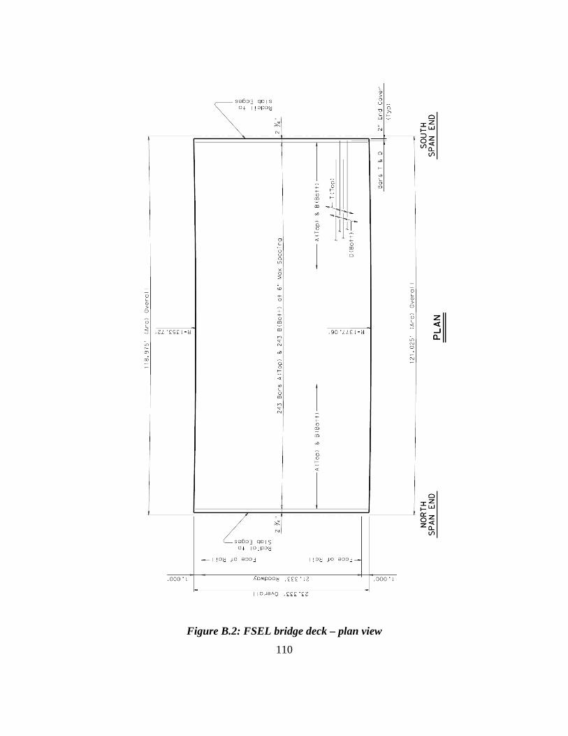
110
Figure B.2: FSEL bridge deck – plan view
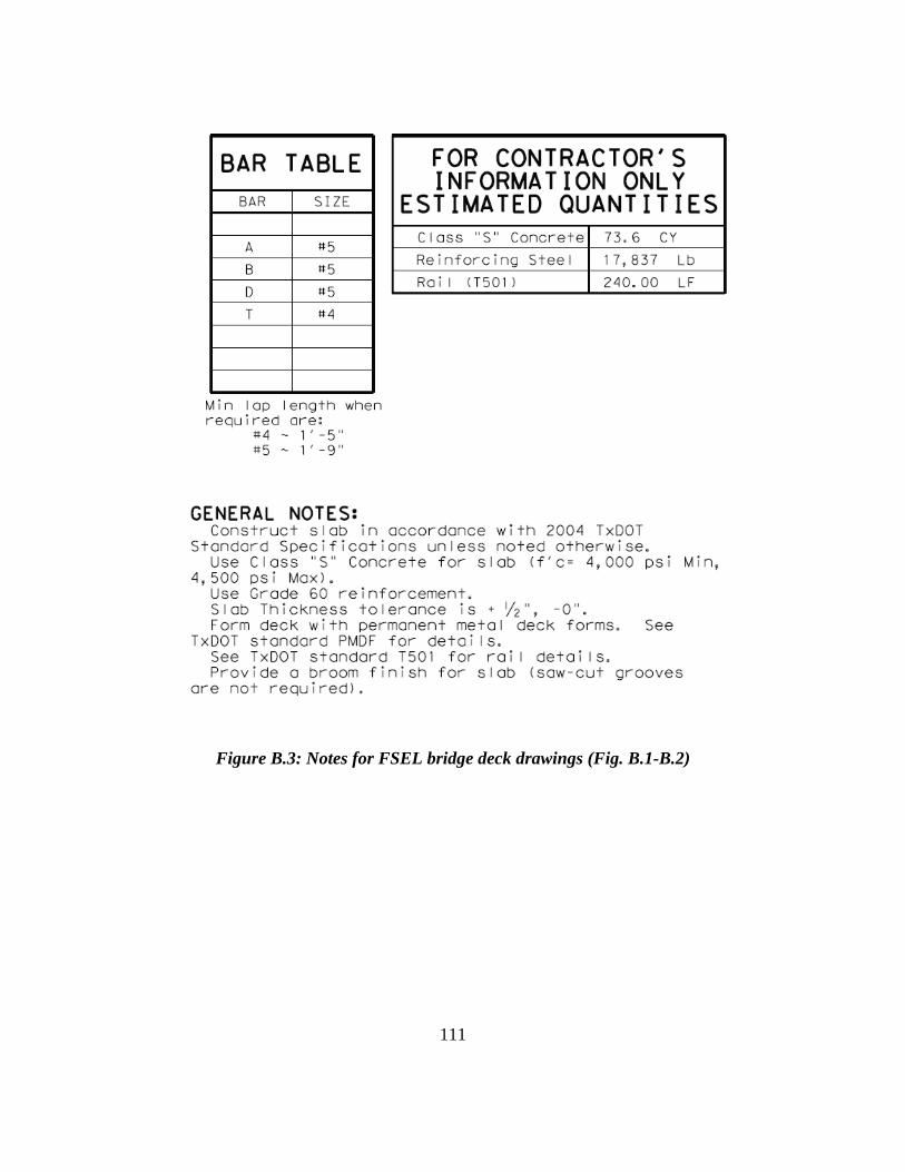
111
Figure B.3: Notes for FSEL bridge deck drawings (Fig. B.1-B.2)
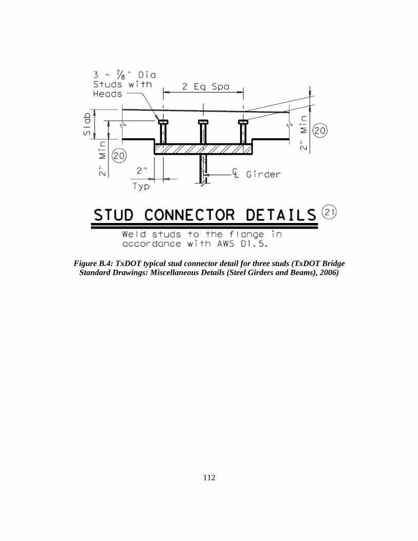
112
Figure B.4: TxDOT typical stud connector detail for three studs (TxDOT Bridge Standard Drawings: Miscellaneous Details (Steel Girders and Beams), 2006)
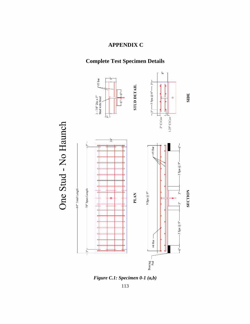
113
APPENDIX C
Complete Test Specimen Details
Figure C.1: Specimen 0-1 (a,b)
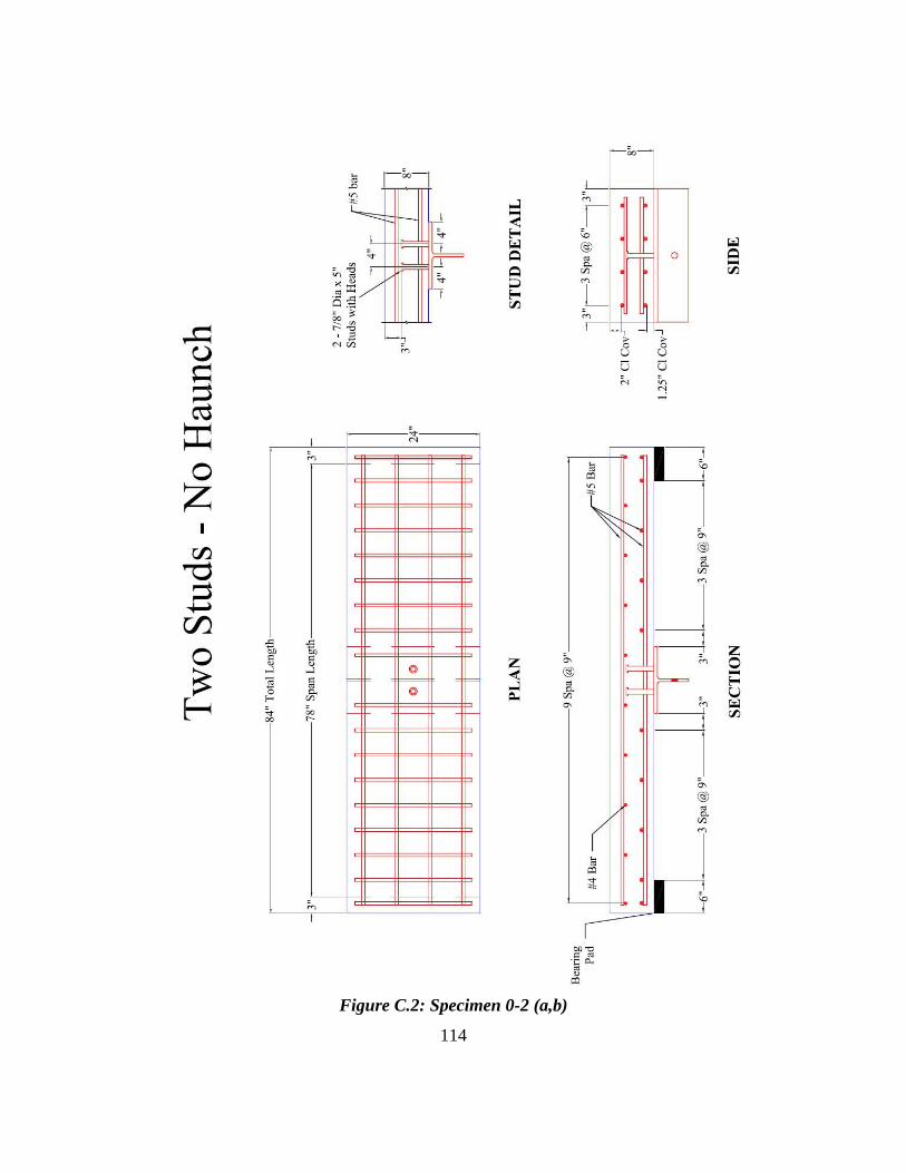
114
Figure C.2: Specimen 0-2 (a,b)
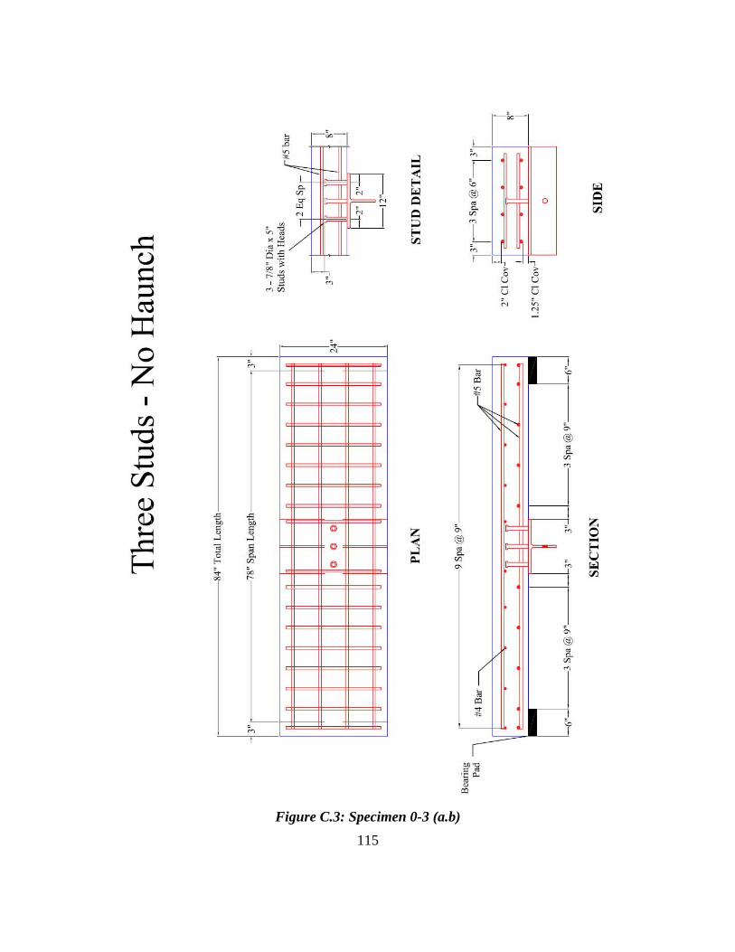
115
Figure C.3: Specimen 0-3 (a.b)
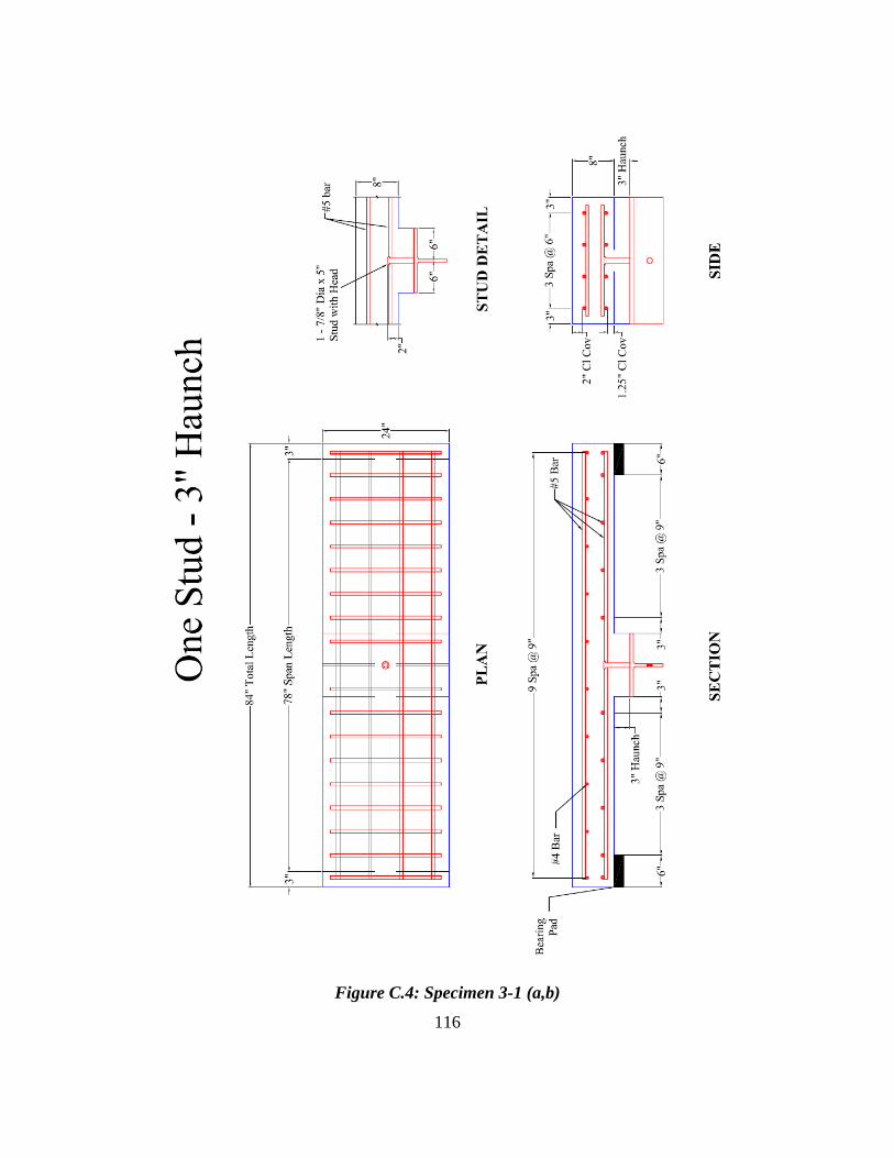
116
Figure C.4: Specimen 3-1 (a,b)
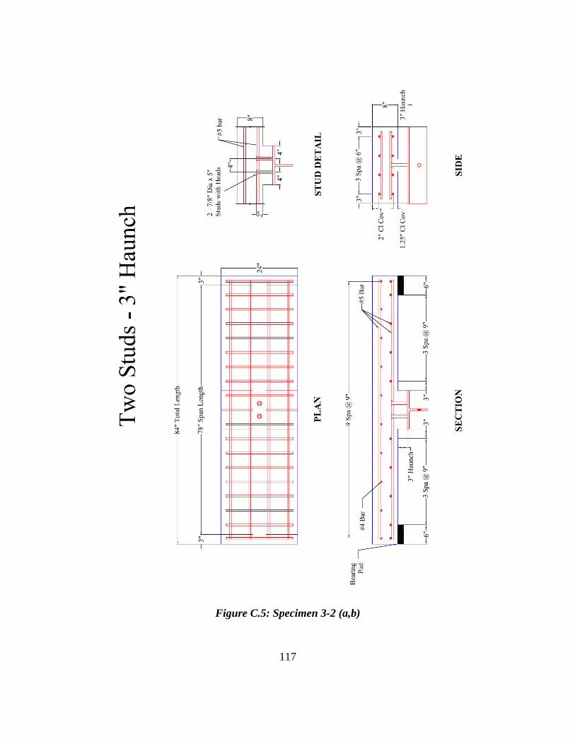
117
Figure C.5: Specimen 3-2 (a,b)
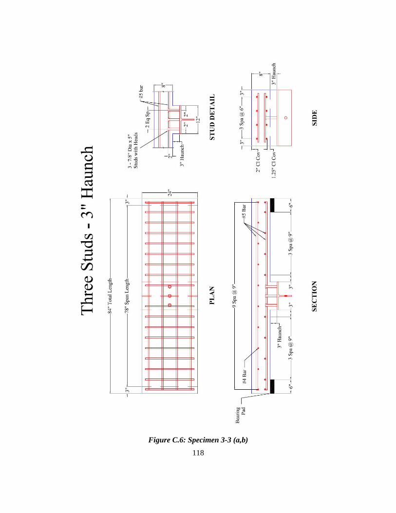
118
Figure C.6: Specimen 3-3 (a,b)
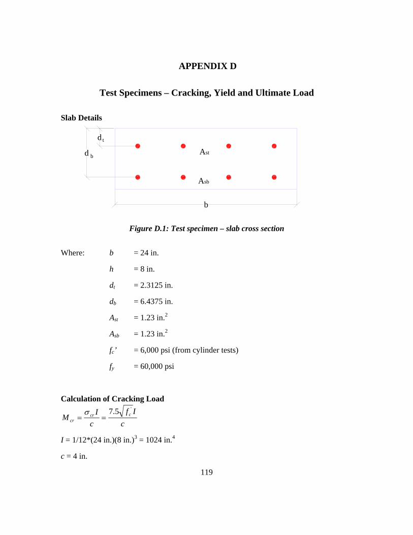
119
APPENDIX D
Test Specimens – Cracking, Yield and Ultimate Load
Slab Details
d
d b
t
Asb
Ast
b
Figure D.1: Test specimen – slab cross section
Where: b = 24 in.
h = 8 in.
dt = 2.3125 in.
db = 6.4375 in.
Ast = 1.23 in.2
Asb = 1.23 in.2
fc’ = 6,000 psi (from cylinder tests)
fy = 60,000 psi
Calculation of Cracking Load
cIf
cI
M ccrcr
'5.7==
σ
I = 1/12*(24 in.)(8 in.)3 = 1024 in.4
c = 4 in.
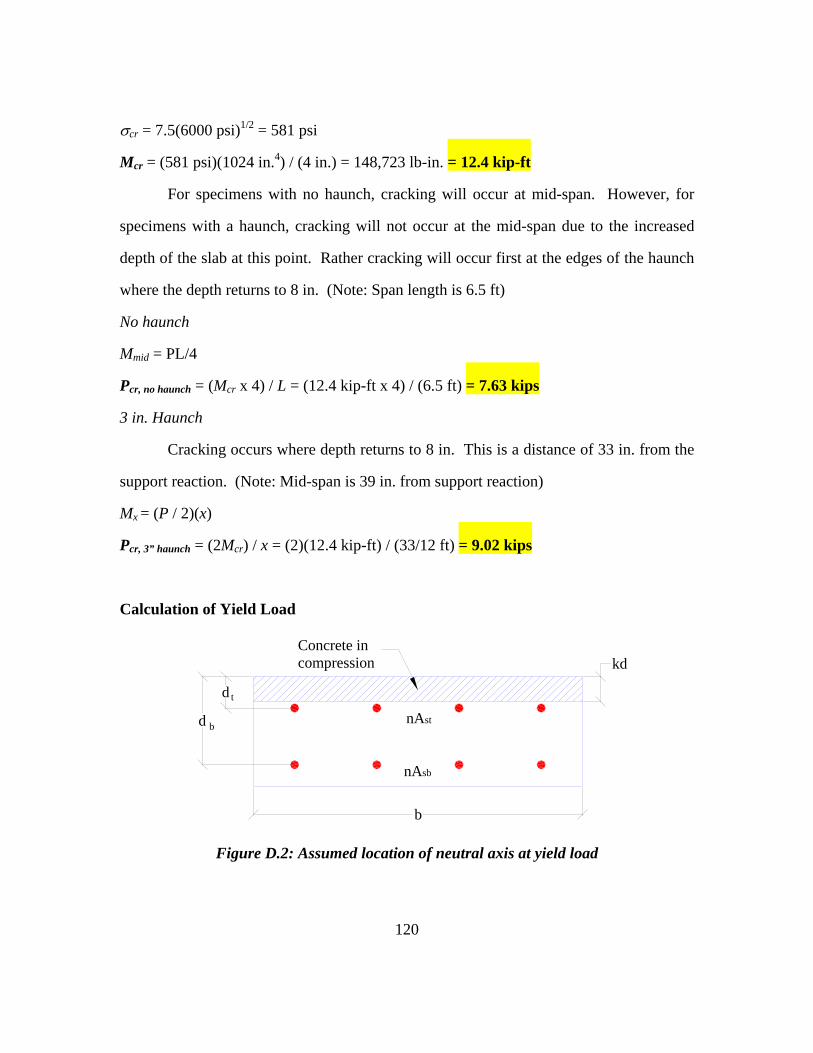
120
σcr = 7.5(6000 psi)1/2 = 581 psi
Mcr = (581 psi)(1024 in.4) / (4 in.) = 148,723 lb-in. = 12.4 kip-ft
For specimens with no haunch, cracking will occur at mid-span. However, for
specimens with a haunch, cracking will not occur at the mid-span due to the increased
depth of the slab at this point. Rather cracking will occur first at the edges of the haunch
where the depth returns to 8 in. (Note: Span length is 6.5 ft)
No haunch
Mmid = PL/4
Pcr, no haunch = (Mcr x 4) / L = (12.4 kip-ft x 4) / (6.5 ft) = 7.63 kips
3 in. Haunch
Cracking occurs where depth returns to 8 in. This is a distance of 33 in. from the
support reaction. (Note: Mid-span is 39 in. from support reaction)
Mx = (P / 2)(x)
Pcr, 3” haunch = (2Mcr) / x = (2)(12.4 kip-ft) / (33/12 ft) = 9.02 kips
Calculation of Yield Load
kdConcrete in compression
d
d b
t
nAsb
nAst
b
Figure D.2: Assumed location of neutral axis at yield load
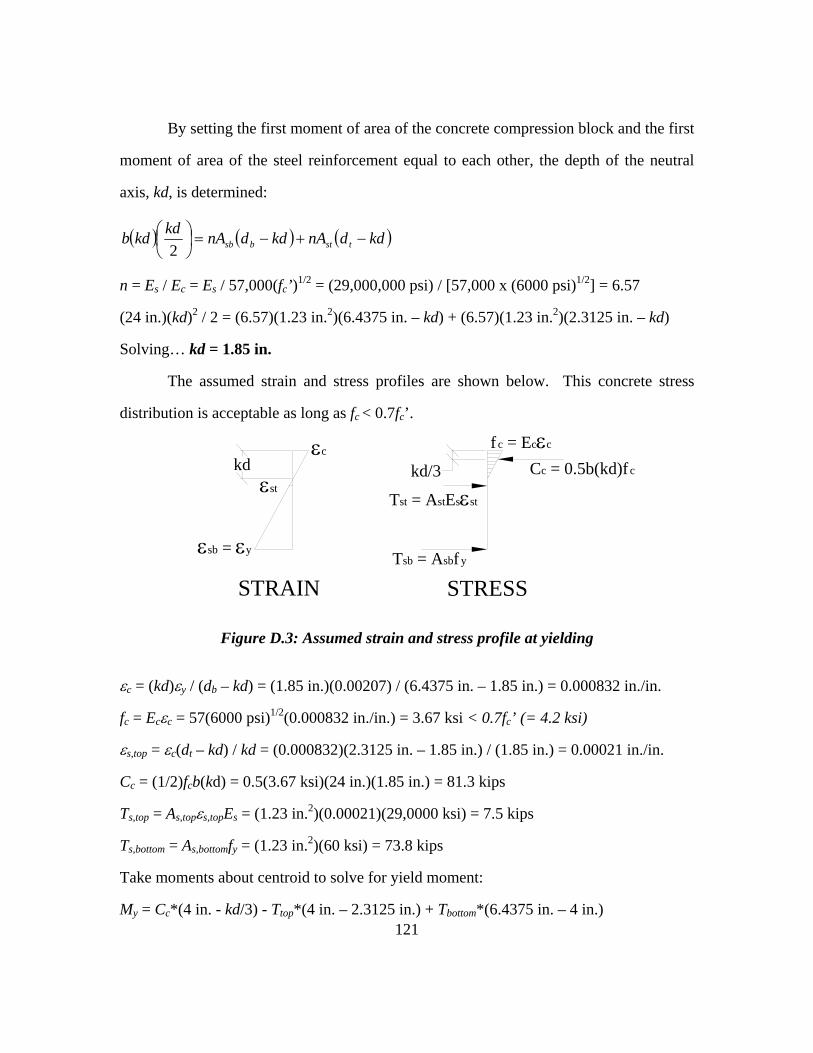
121
By setting the first moment of area of the concrete compression block and the first
moment of area of the steel reinforcement equal to each other, the depth of the neutral
axis, kd, is determined:
( ) ( ) ( )kddnAkddnAkdkdb tstbsb −+−=⎟⎠⎞
⎜⎝⎛
2
n = Es / Ec = Es / 57,000(fc’)1/2 = (29,000,000 psi) / [57,000 x (6000 psi)1/2] = 6.57
(24 in.)(kd)2 / 2 = (6.57)(1.23 in.2)(6.4375 in. – kd) + (6.57)(1.23 in.2)(2.3125 in. – kd)
Solving… kd = 1.85 in.
The assumed strain and stress profiles are shown below. This concrete stress
distribution is acceptable as long as fc < 0.7fc’.
εsb = εy
εst
εc kd
Tsb = Asbf y
kd/3
Tst = AstEsεst
f c = Ecεc
Cc = 0.5b(kd)fc
STRAIN STRESS
Figure D.3: Assumed strain and stress profile at yielding
εc = (kd)εy / (db – kd) = (1.85 in.)(0.00207) / (6.4375 in. – 1.85 in.) = 0.000832 in./in.
fc = Ecεc = 57(6000 psi)1/2(0.000832 in./in.) = 3.67 ksi < 0.7fc’ (= 4.2 ksi)
εs,top = εc(dt – kd) / kd = (0.000832)(2.3125 in. – 1.85 in.) / (1.85 in.) = 0.00021 in./in.
Cc = (1/2)fcb(kd) = 0.5(3.67 ksi)(24 in.)(1.85 in.) = 81.3 kips
Ts,top = As,topεs,topEs = (1.23 in.2)(0.00021)(29,0000 ksi) = 7.5 kips
Ts,bottom = As,bottomfy = (1.23 in.2)(60 ksi) = 73.8 kips
Take moments about centroid to solve for yield moment:
My = Cc*(4 in. - kd/3) - Ttop*(4 in. – 2.3125 in.) + Tbottom*(6.4375 in. – 4 in.)
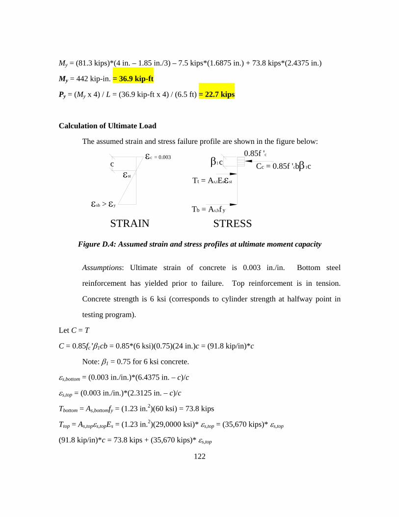
122
My = (81.3 kips)*(4 in. – 1.85 in./3) – 7.5 kips*(1.6875 in.) + 73.8 kips*(2.4375 in.)
My = 442 kip-in. = 36.9 kip-ft
Py = (My x 4) / L = (36.9 kip-ft x 4) / (6.5 ft) = 22.7 kips
Calculation of Ultimate Load
The assumed strain and stress failure profile are shown in the figure below:
εsb > εy
εst
εc = 0.003 c
Tb = As,bf y
Tt = As,tEsεst
0.85f 'c Cc = 0.85f 'cbβ1c
STRAIN STRESS
β1c
Figure D.4: Assumed strain and stress profiles at ultimate moment capacity
Assumptions: Ultimate strain of concrete is 0.003 in./in. Bottom steel
reinforcement has yielded prior to failure. Top reinforcement is in tension.
Concrete strength is 6 ksi (corresponds to cylinder strength at halfway point in
testing program).
Let C = T
C = 0.85fc’β1cb = 0.85*(6 ksi)(0.75)(24 in.)c = (91.8 kip/in)*c
Note: β1 = 0.75 for 6 ksi concrete.
εs,bottom = (0.003 in./in.)*(6.4375 in. – c)/c
εs,top = (0.003 in./in.)*(2.3125 in. – c)/c
Tbottom = As,bottomfy = (1.23 in.2)(60 ksi) = 73.8 kips
Ttop = As,topεs,topEs = (1.23 in.2)(29,0000 ksi)* εs,top = (35,670 kips)* εs,top
(91.8 kip/in)*c = 73.8 kips + (35,670 kips)* εs,top
123
(91.8 kip/in)*c = 73.8 kips + (35,670 kips)* (0.003 in./in.)*(2.3125 in. – c)/c
Iterate until the neutral axis depth is found.
Solving: c = 1.47 in.
εs,bottom = 0.0101 > Yield strain (= 0.00207 for 60 ksi)
εs,top = 0.0017 < Yield strain
C = 135.0 kips
Ttop = 61.2 kips
Take moments about centroid to solve for nominal moment capacity.
Mn = C*(4 in. - β1c/2) - Ttop*(4 in. – 2.3125 in.) + Tbottom*(6.4375 in. – 4 in.)
Mn = (135 kip)*(4 in. – 0.75*1.47 in./2) – 61.2 kip*(1.6875 in.) + 73.8 kip*(2.4375 in.)
Mn = 542 kip-in. = 45.2 kip-ft
Pn = (Mn x 4) / L = (45.2 kip-ft x 4) / (6.5 ft) = 27.8 kips
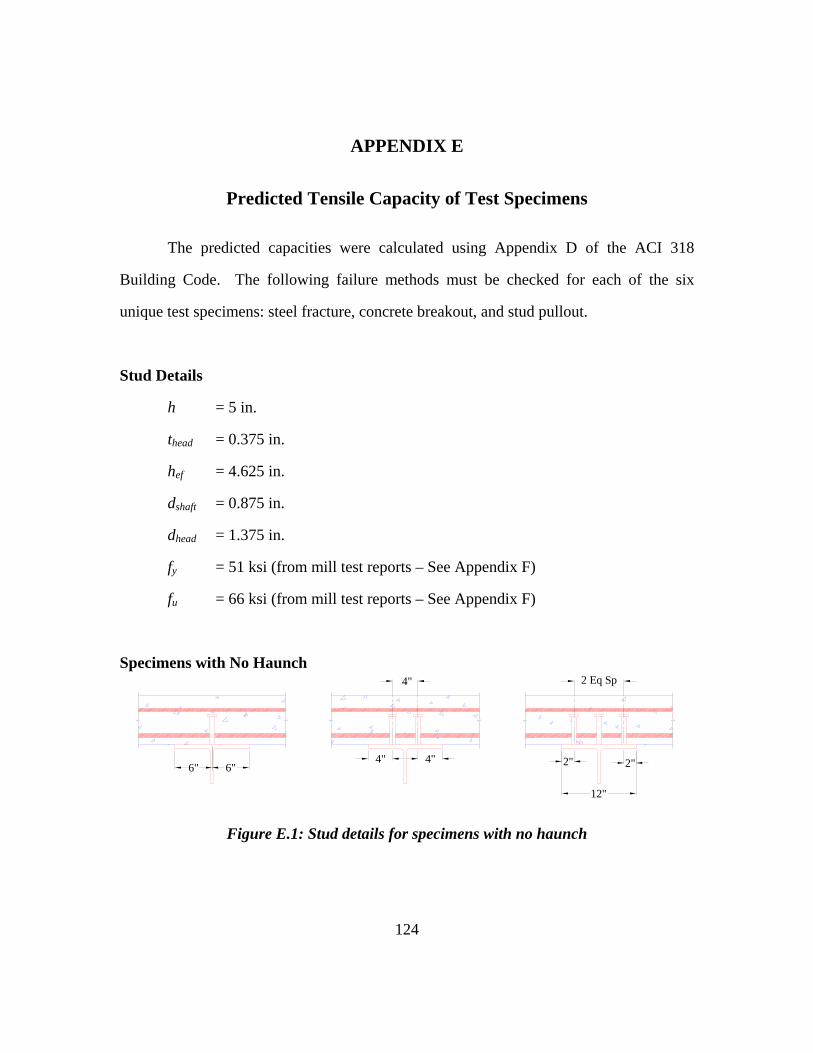
124
APPENDIX E
Predicted Tensile Capacity of Test Specimens
The predicted capacities were calculated using Appendix D of the ACI 318
Building Code. The following failure methods must be checked for each of the six
unique test specimens: steel fracture, concrete breakout, and stud pullout.
Stud Details
h = 5 in.
thead = 0.375 in.
hef = 4.625 in.
dshaft = 0.875 in.
dhead = 1.375 in.
fy = 51 ksi (from mill test reports – See Appendix F)
fu = 66 ksi (from mill test reports – See Appendix F)
Specimens with No Haunch 4"
4" 4" 2" 2"
2 Eq Sp
12"
6" 6"
Figure E.1: Stud details for specimens with no haunch
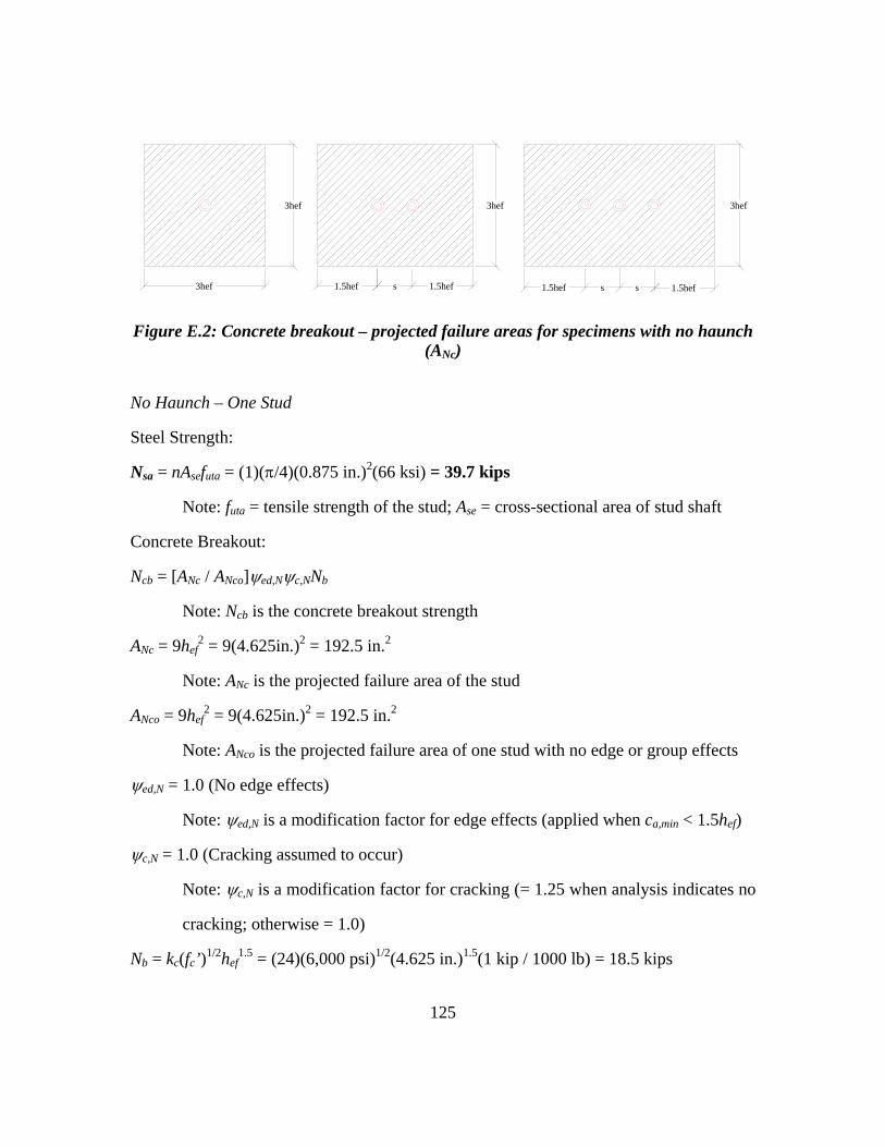
125
3hef
s s1.5hef 1.5hef
3hef
s 1.5hef1.5hef
3hef
3hef
Figure E.2: Concrete breakout – projected failure areas for specimens with no haunch (ANc)
No Haunch – One Stud
Steel Strength:
Nsa = nAsefuta = (1)(π/4)(0.875 in.)2(66 ksi) = 39.7 kips
Note: futa = tensile strength of the stud; Ase = cross-sectional area of stud shaft
Concrete Breakout:
Ncb = [ANc / ANco]ψed,Nψc,NNb
Note: Ncb is the concrete breakout strength
ANc = 9hef2 = 9(4.625in.)2 = 192.5 in.2
Note: ANc is the projected failure area of the stud
ANco = 9hef2 = 9(4.625in.)2 = 192.5 in.2
Note: ANco is the projected failure area of one stud with no edge or group effects
ψed,N = 1.0 (No edge effects)
Note: ψed,N is a modification factor for edge effects (applied when ca,min < 1.5hef)
ψc,N = 1.0 (Cracking assumed to occur)
Note: ψc,N is a modification factor for cracking (= 1.25 when analysis indicates no
cracking; otherwise = 1.0)
Nb = kc(fc’)1/2hef1.5 = (24)(6,000 psi)1/2(4.625 in.)1.5(1 kip / 1000 lb) = 18.5 kips
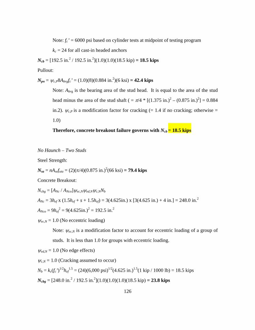
126
Note: fc’ = 6000 psi based on cylinder tests at midpoint of testing program
kc = 24 for all cast-in headed anchors
Ncb = [192.5 in.2 / 192.5 in.2](1.0)(1.0)(18.5 kip) = 18.5 kips
Pullout:
Npn = ψc,P8Abrgfc’ = (1.0)(8)(0.884 in.2)(6 ksi) = 42.4 kips
Note: Abrg is the bearing area of the stud head. It is equal to the area of the stud
head minus the area of the stud shaft ( = π/4 * [(1.375 in.)2 – (0.875 in.)2] = 0.884
in.2). ψc,P is a modification factor for cracking (= 1.4 if no cracking; otherwise =
1.0)
Therefore, concrete breakout failure governs with Ncb = 18.5 kips
No Haunch – Two Studs
Steel Strength:
Nsa = nAsefuta = (2)(π/4)(0.875 in.)2(66 ksi) = 79.4 kips
Concrete Breakout:
Ncbg = [ANc / ANco]ψec,Nψed,Nψc,NNb
ANc = 3hef x (1.5hef + s + 1.5hef) = 3(4.625in.) x [3(4.625 in.) + 4 in.] = 248.0 in.2
ANco = 9hef2 = 9(4.625in.)2 = 192.5 in.2
ψec,N = 1.0 (No eccentric loading)
Note: ψec,N is a modification factor to account for eccentric loading of a group of
studs. It is less than 1.0 for groups with eccentric loading.
ψed,N = 1.0 (No edge effects)
ψc,N = 1.0 (Cracking assumed to occur)
Nb = kc(fc’)1/2hef1.5 = (24)(6,000 psi)1/2(4.625 in.)1.5(1 kip / 1000 lb) = 18.5 kips
Ncbg = [248.0 in.2 / 192.5 in.2](1.0)(1.0)(1.0)(18.5 kip) = 23.8 kips
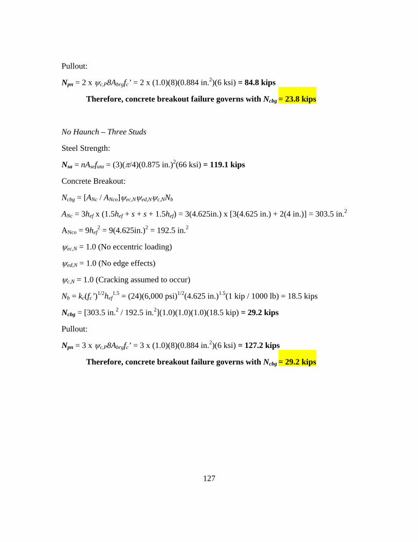
127
Pullout:
Npn = 2 x ψc,P8Abrgfc’ = 2 x (1.0)(8)(0.884 in.2)(6 ksi) = 84.8 kips
Therefore, concrete breakout failure governs with Ncbg = 23.8 kips
No Haunch – Three Studs
Steel Strength:
Nsa = nAsefuta = (3)(π/4)(0.875 in.)2(66 ksi) = 119.1 kips
Concrete Breakout:
Ncbg = [ANc / ANco]ψec,Nψed,Nψc,NNb
ANc = 3hef x (1.5hef + s + s + 1.5hef) = 3(4.625in.) x [3(4.625 in.) + 2(4 in.)] = 303.5 in.2
ANco = 9hef2 = 9(4.625in.)2 = 192.5 in.2
ψec,N = 1.0 (No eccentric loading)
ψed,N = 1.0 (No edge effects)
ψc,N = 1.0 (Cracking assumed to occur)
Nb = kc(fc’)1/2hef1.5 = (24)(6,000 psi)1/2(4.625 in.)1.5(1 kip / 1000 lb) = 18.5 kips
Ncbg = [303.5 in.2 / 192.5 in.2](1.0)(1.0)(1.0)(18.5 kip) = 29.2 kips
Pullout:
Npn = 3 x ψc,P8Abrgfc’ = 3 x (1.0)(8)(0.884 in.2)(6 ksi) = 127.2 kips
Therefore, concrete breakout failure governs with Ncbg = 29.2 kips
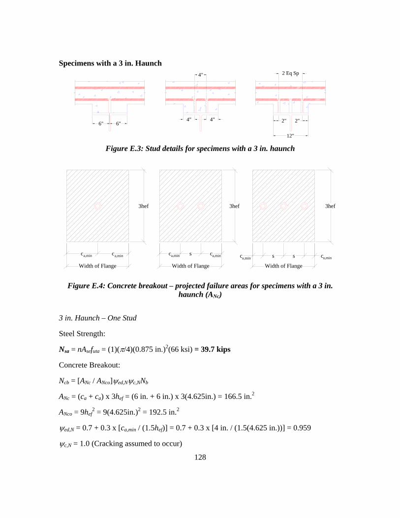
128
Specimens with a 3 in. Haunch 4" 2 Eq Sp
4" 4" 2" 2"
12"
6" 6"
Figure E.3: Stud details for specimens with a 3 in. haunch
3hef
s sc c
3hef
s cc
3hef
cc
Width of Flange Width of Flange Width of Flange
a,min a,min a,min a,min a,min a,min
Figure E.4: Concrete breakout – projected failure areas for specimens with a 3 in. haunch (ANc)
3 in. Haunch – One Stud
Steel Strength:
Nsa = nAsefuta = (1)(π/4)(0.875 in.)2(66 ksi) = 39.7 kips
Concrete Breakout:
Ncb = [ANc / ANco]ψed,Nψc,NNb
ANc = (ca + ca) x 3hef = (6 in. + 6 in.) x 3(4.625in.) = 166.5 in.2
ANco = 9hef2 = 9(4.625in.)2 = 192.5 in.2
ψed,N = 0.7 + 0.3 x [ca,min / (1.5hef)] = 0.7 + 0.3 x [4 in. / (1.5(4.625 in.))] = 0.959
ψc,N = 1.0 (Cracking assumed to occur)
129
Nb = kc(fc’)1/2hef1.5 = (24)(6,000 psi)1/2(4.625 in.)1.5(1 kip / 1000 lb) = 18.5 kips
Ncb = [166.5 in.2 / 192.5 in.2](0.959)(1.0)(18.5 kip) = 15.3 kips
Pullout:
Npn = ψc,P8Abrgfc’ = (1.0)(8)(0.884 in.2)(6 ksi) = 42.4 kips
Therefore, concrete breakout failure governs with Ncb = 15.3 kips
3 in. Haunch – Two Studs
Steel Strength:
Nsa = nAsefuta = (2)(π/4)(0.875 in.)2(66 ksi) = 79.4 kips
Concrete Breakout:
Ncb = [ANc / ANco]ψed,Nψc,NNb
ANc = (ca + s + ca) x 3hef = (4 in. + 4 in. + 4 in.) x 3(4.625in.) = 166.5 in.2
ANco = 9hef2 = 9(4.625in.)2 = 192.5 in.2
ψed,N = 0.7 + 0.3 x [ca,min / (1.5hef)] = 0.7 + 0.3 x [4 in. / (1.5(4.625 in.))] = 0.873
ψc,N = 1.0 (Cracking assumed to occur)
Nb = kc(fc’)1/2hef1.5 = (24)(6,000 psi)1/2(4.625 in.)1.5(1 kip / 1000 lb) = 18.5 kips
Ncb = [166.5 in.2 / 192.5 in.2](0.873)(1.0)(18.5 kip) = 14.0 kips
Pullout:
Npn = 2 x ψc,P8Abrgfc’ = 2 x (1.0)(8)(0.884 in.2)(6 ksi) = 84.8 kips
Therefore, concrete breakout failure governs with Ncbg = 14.0 kips
3 in. Haunch – Three Studs
Steel Strength:
Nsa = nAsefuta = (3)(π/4)(0.875 in.)2(66 ksi) = 119.1 kips
Concrete Breakout:
130
Ncb = [ANc / ANco]ψed,Nψc,NNb
ANc = (ca + s + s + ca) x 3hef = (2 in. + 4 in. + 4 in. + 2 in.) x 3(4.625in.) = 166.5 in.2
ANco = 9hef2 = 9(4.625in.)2 = 192.5 in.2
ψed,N = 0.7 + 0.3 x [ca,min / (1.5hef)] = 0.7 + 0.3 x [2 in. / (1.5(4.625 in.))] = 0.786
ψc,N = 1.0 (Cracking assumed to occur)
Nb = kc(fc’)1/2hef1.5 = (24)(6,000 psi)1/2(4.625 in.)1.5(1 kip / 1000 lb) = 18.5 kips
Ncb = [166.5 in.2 / 192.5 in.2](0.786)(1.0)(18.5 kip) = 12.6 kips
Pullout:
Npn = 3 x ψc,P8Abrgfc’ = 2 x (1.0)(8)(0.884 in.2)(6 ksi) = 127.2 kips
Therefore, concrete breakout failure governs with Ncbg = 12.6 kips
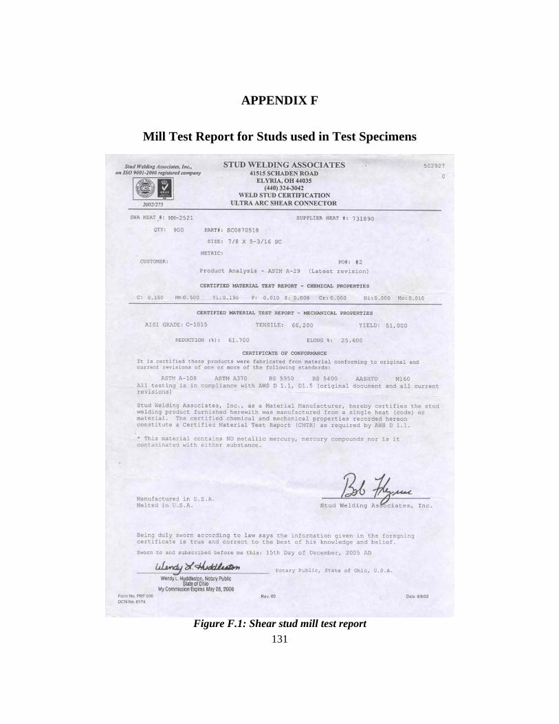
131
APPENDIX F
Mill Test Report for Studs used in Test Specimens
Figure F.1: Shear stud mill test report
132
REFERENCES
ACI Committee 318. (2005). Building Code Requirements for Structural Concrete (ACI 318-05) and Commentary (ACI 318R-05). American Concrete Institute, Farmington Hills, MI.
American Association of State Highway Transportation Officials. (2004). AASHTO LRFD Bridge Design Specifications. Washington, D.C.
American Association of State Highway Transportation Officials/American Welding Society. (2002). AASHTO/AWS D1.5M/D1.5:2002 Bridge Welding Code. AASHTO/AWS, Washington D.C./Miami, FL.
Connor, Robert J., Dexter, Robert, and Mahmoud, Hussam. (2005). “Inspection and Management of Bridges with Fracture-Critical Details.” National Cooperative Highway Research Program Synthesis 354. Transportation Research Board, National Academy Press, Washington, D.C.
Daniels, J. H., Kim, W., and Wilson, J. L. (1989). “Recommended Guidelines for Redundancy Design and Rating of Two-Girder Steel Bridges.” National Cooperative Highway Research Program Report 319. Transportation Research Board, National Academy Press, Washington, D.C.
Eligehausen, Rolf and Balogh, Tamas. (1995). “Behavior of Fasteners Loaded in Tension in Cracked Reinforced Concrete.” ACI Structural Journal, vol. 92, no. 3, pp. 365-379.
Fuchs, Werner, Eligehausen, Rolf, and Breen, John E. (1995). “Concrete Capacity Design (CCD) Approach for Fastening to Concrete.” ACI Structural Journal, vol. 92, no. 1, pp. 73-94.
Ghosn, M. and Moses, F. (1998). “Redundancy in Highway Bridge Superstructures.” National Cooperative Highway Research Program Report 406. Transportation Research Board, National Academy Press, Washington, D.C.
Texas Department of Transportation. (2001). Bridge Design Manual.
Texas Department of Transportation. (2001). Bridge Detailing Manual.
Texas Department of Transportation. (2006). Bridge Standard Drawings.
Shirvani, Mansour, Klingner, Richard E., and Graves III, Herman L. (2004). “Breakout Capacity of Anchors in Concrete – Part 1: Tension.” ACI Structural Journal, vol. 101, no. 6, pp. 812-820.
133
VITA
James Patrick Sutton was born in West Islip, New York on July 4, 1983, the son
of James Christopher and Mary Katherine Sutton. He is the brother of Erin, Patrick and
Mary Beth Sutton. He attended Regis High School in New York, New York where he
graduated in June 2001. He obtained his Bachelor of Science in Civil Engineering from
Villanova University in May 2005 and entered the Graduate School at the University of
Texas in August 2005 to pursue a Master of Science in Engineering degree. While at the
University of Texas, he worked as a Graduate Research Assistant at the Phil M. Ferguson
Structural Engineering Laboratory. He completed his M.S.E. in May 2007.
Permanent address: 15 Creek Court
Easton, Pennsylvania 18040
This thesis was typed by the author.