Copyright © Cengage Learning. All rights reserved. 14 Goodness-of-Fit Tests and Categorical Data Analysis

Copyright © Cengage Learning. All rights reserved.

14Goodness-of-Fit Tests and Categorical Data

Analysis

Copyright © Cengage Learning. All rights reserved.

14.1Goodness-of-Fit Tests When

Category ProbabilitiesAre Completely Specified

3

Goodness-of-Fit Tests When Category Probabilities Are Completely Specified

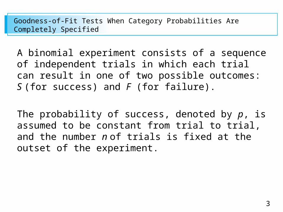
A binomial experiment consists of a sequence of independent trials in which each trial can result in one of two possible outcomes: S (for success) and F (for failure).

The probability of success, denoted by p, is assumed to be constant from trial to trial, and the number n of trials is fixed at the outset of the experiment.

4


We already presented a large-sample z test for testing H0: p = p0.

Notice that this null hypothesis specifies both P(S) and P(F), since if

P(S) = p0, then P(F) = 1 – p0.

Denoting P(F) by q and 1 – p0 by q0, the null hypothesis can alternatively be written as

H0: p = p0, q = q0.

5


The z test is two-tailed when the alternative of interest isp ≠ p0. A multinomial experiment generalizes a binomial experiment by allowing each trial to result in one of k possible outcomes, where k > 2.

For example, suppose a store accepts three different types of credit cards. A multinomial experiment would result from observing the type of credit card used—type 1, type 2, or type 3—by each of the next n customers who pay with a credit card.

In general, we will refer to the k possible outcomes on any given trial as categories, and pi will denote the probability that a trial results in category i.

6


If the experiment consists of selecting n individuals or objects from a population and categorizing each one, then pi is the proportion of the population falling in the ith category (such an experiment will be approximately multinomial provided that n is much smaller than the population size).

The null hypothesis of interest will specify the value of each pi.

For example, in the case k = 3, we might have H0: p1 = .5, p2 = .3, p3 = .2.

7


The alternative hypothesis will state that H0 is not true—that is, that at least one of the pi’s has a value different from that asserted by H0 (in which case at least two must be different, since they sum to 1).

The symbol pi0 will represent the value of pi claimed by the null hypothesis. In the example just given, p10 = .5, p20 = .3, and p30 = .2.

Before the multinomial experiment is performed, the number of trials that will result in category i(i = 1,2,…, or k) is a random variable—just as the number of successes and the number of failures in a binomial experiment are random variables.

8


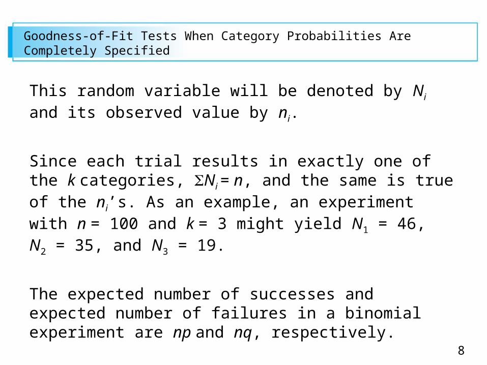
This random variable will be denoted by Ni and its observed value by ni.

Since each trial results in exactly one of the k categories, Ni = n, and the same is true of the ni’s. As an example, an experiment with n = 100 and k = 3 might yield N1 = 46, N2 = 35, and N3 = 19.

The expected number of successes and expected number of failures in a binomial experiment are np and nq, respectively.

9


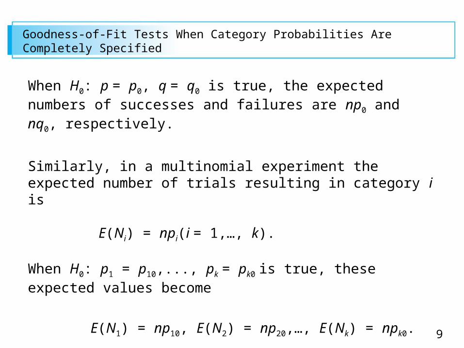
When H0: p = p0, q = q0 is true, the expected numbers of successes and failures are np0 and nq0, respectively.

Similarly, in a multinomial experiment the expected number of trials resulting in category i is

E(Ni) = npi(i = 1,…, k).

When H0: p1 = p10,..., pk = pk0 is true, these expected values become

E(N1) = np10, E(N2) = np20,…, E(Nk) = npk0.

10


For the case k = 3,

H0: p1 = .5,

p2 = .3, p3 = .2, and

n = 100, the expected frequencies when H0 is true are

E(N1) = 100(.5) = 50,

E(N2) = 30, and

E(N3) = 20.

11


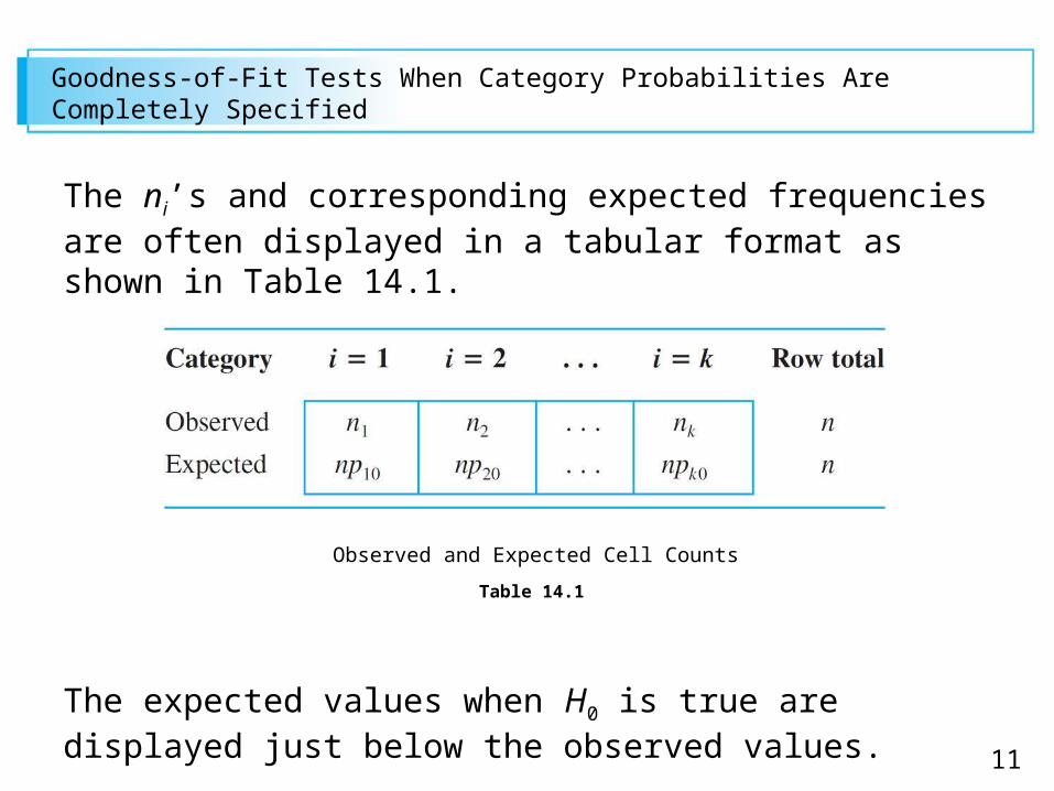
The ni’s and corresponding expected frequencies are often displayed in a tabular format as shown in Table 14.1.

The expected values when H0 is true are displayed just below the observed values.

Table 14.1

Observed and Expected Cell Counts

12


The Ni’s and ni’s are usually referred to as observed cell counts (or observed cell frequencies), and np10, np20,…, npk0 are the corresponding expected cell counts under H0.

The ni’s should all be reasonably close to the corresponding npi0’s when H0 is true.

On the other hand, several of the observed counts should differ substantially from these expected counts when the actual values of the pi’s differ markedly from what the null hypothesis asserts.

13


The test procedure involves assessing the discrepancy between the ni’s and the npi0’s, with H0 being rejected when the discrepancy is sufficiently large.

It is natural to base a measure of discrepancy on the squared deviations (n1 – np10)2, (n2 – np20)2,…, (nk – npk0)2.

A seemingly sensible way to combine these into an overall measure is to add them together to obtain (ni – npi0)2.

However, suppose np10 = 100 and np20 = 10. Then if n1 = 95 and n2 = 5, the two categories contribute the same squared deviations to the proposed measure.

14


Yet n1 is only 5% less than what would be expected when H0 is true, whereas n2 is 50% less.

To take relative magnitudes of the deviations into account, each squared deviation is divided by the corresponding expected count.

Before giving a more detailed description, we must discuss a type of probability distribution called the chi-squared distribution.

15


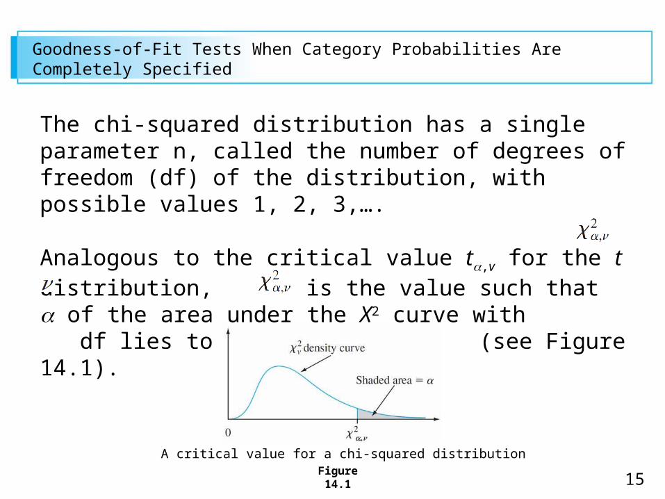
The chi-squared distribution has a single parameter n, called the number of degrees of freedom (df) of the distribution, with possible values 1, 2, 3,….

Analogous to the critical value t,v for the t distribution, is the value such that of the area under the X2 curve with df lies to the right of (see Figure 14.1).

Figure 14.1

A critical value for a chi-squared distribution

16


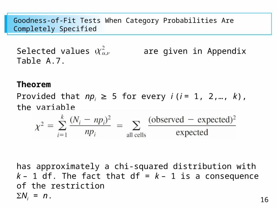
Selected values of are given in Appendix Table A.7.

Theorem

Provided that npi 5 for every i (i = 1, 2,…, k), the variable

has approximately a chi-squared distribution with k – 1 df. The fact that df = k – 1 is a consequence of the restrictionNi = n.

17


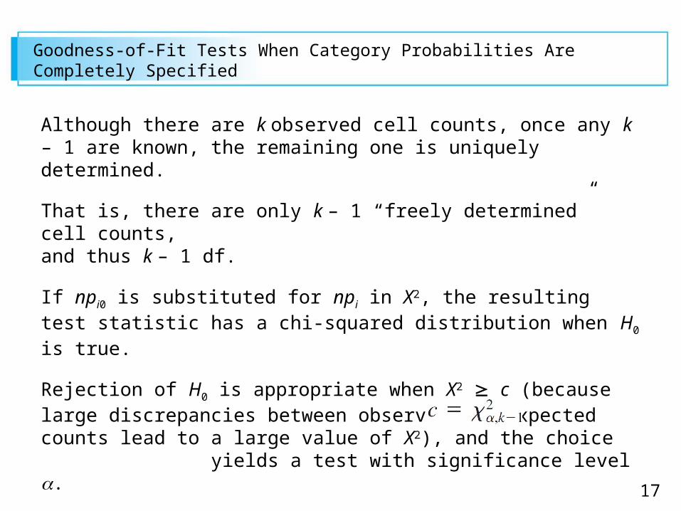
Although there are k observed cell counts, once any k – 1 are known, the remaining one is uniquely determined.

That is, there are only k – 1 “freely determined” cell counts,and thus k – 1 df.

If npi0 is substituted for npi in X2, the resulting test statistic has a chi-squared distribution when H0 is true.

Rejection of H0 is appropriate when X2 c (because large discrepancies between observed and expected counts lead to a large value of X2), and the choice yields a test with significance level .

18


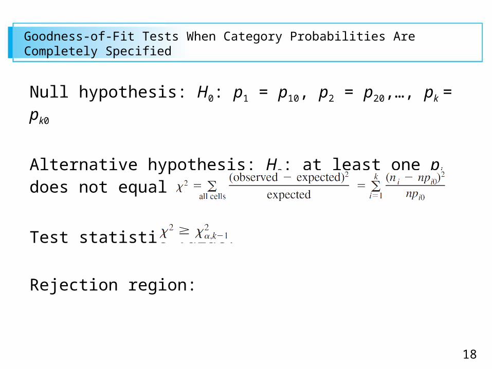
Null hypothesis: H0: p1 = p10, p2 = p20,…, pk = pk0

Alternative hypothesis: Ha: at least one pi does not equal pi0

Test statistic value:

Rejection region:

19

Example 1

If we focus on two different characteristics of an organism, each controlled by a single gene, and cross a pure strain having genotype AABB with a pure strain having genotype aabb (capital letters denoting dominant alleles and small letters recessive alleles), the resulting genotype will be AaBb.

If these first-generation organisms are then crossed among themselves (a dihybrid cross), there will be four phenotypes depending on whether a dominant allele of either type is present.

20

Example 1

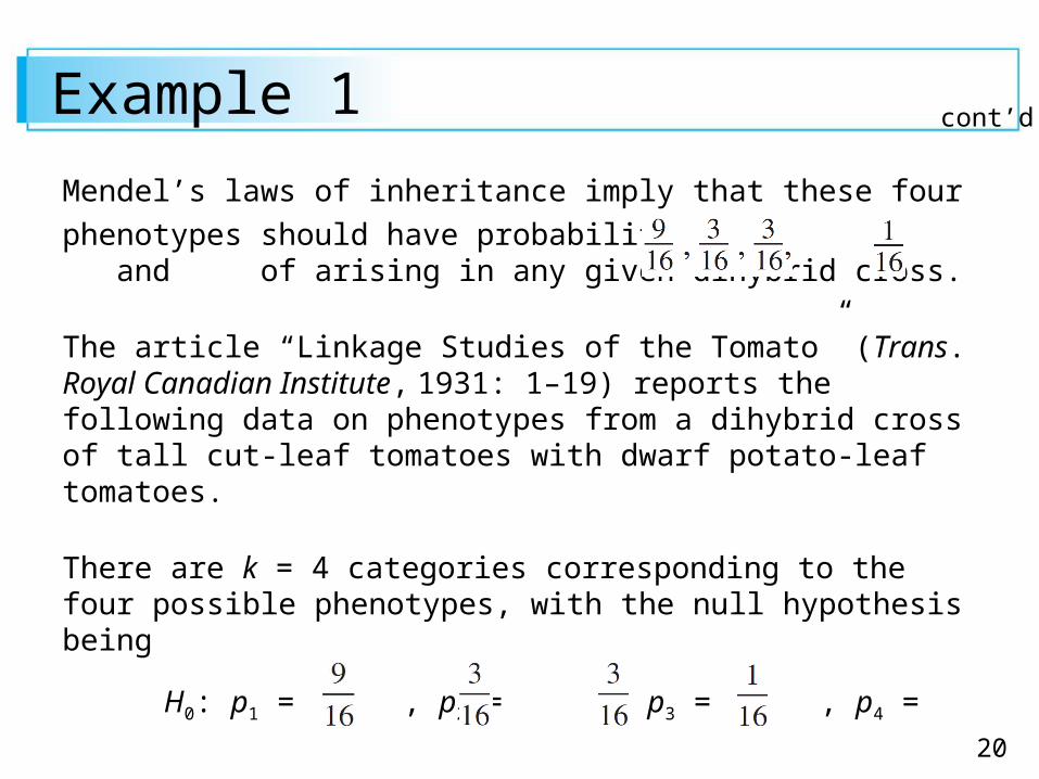
Mendel’s laws of inheritance imply that these four

phenotypes should have probabilities and of arising in any given dihybrid cross.

The article “Linkage Studies of the Tomato” (Trans. Royal Canadian Institute, 1931: 1–19) reports the following data on phenotypes from a dihybrid cross of tall cut-leaf tomatoes with dwarf potato-leaf tomatoes.

There are k = 4 categories corresponding to the four possible phenotypes, with the null hypothesis being

H0: p1 = , p2 = , p3 = , p4 =

cont’d

21

Example 1

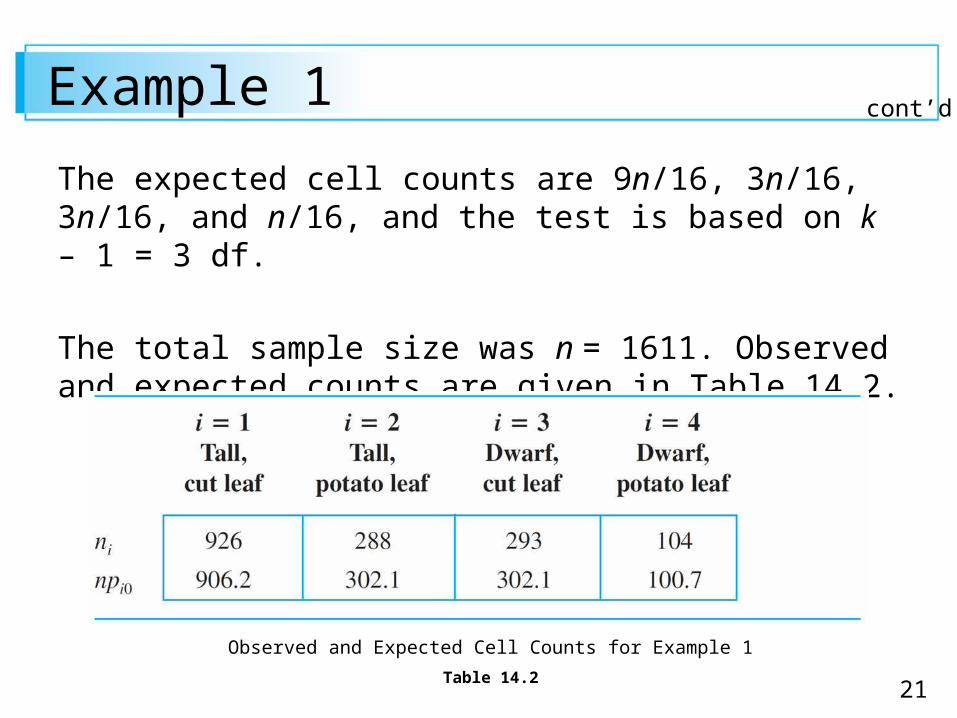
The expected cell counts are 9n/16, 3n/16, 3n/16, and n/16, and the test is based on k – 1 = 3 df.

The total sample size was n = 1611. Observed and expected counts are given in Table 14.2.

Table 14.2

Observed and Expected Cell Counts for Example 1

cont’d

22

Example 1

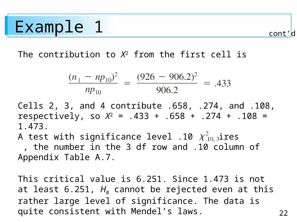
The contribution to X2 from the first cell is

Cells 2, 3, and 4 contribute .658, .274, and .108, respectively, so X2 = .433 + .658 + .274 + .108 = 1.473. A test with significance level .10 requires , the number in the 3 df row and .10 column of Appendix Table A.7.

This critical value is 6.251. Since 1.473 is not at least 6.251, H0 cannot be rejected even at this rather large level of significance. The data is quite consistent with Mendel’s laws.

cont’d

23


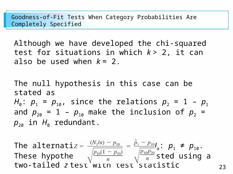
Although we have developed the chi-squared test for situations in which k > 2, it can also be used when k = 2.

The null hypothesis in this case can be stated as H0: p1 = p10, since the relations p2 = 1 – p1 and p20 = 1 – p10 make the inclusion of p2 = p20 in H0 redundant.

The alternative hypothesis is Ha: p1 ≠ p10. These hypotheses can also be tested using a two-tailed z test with test statistic

24


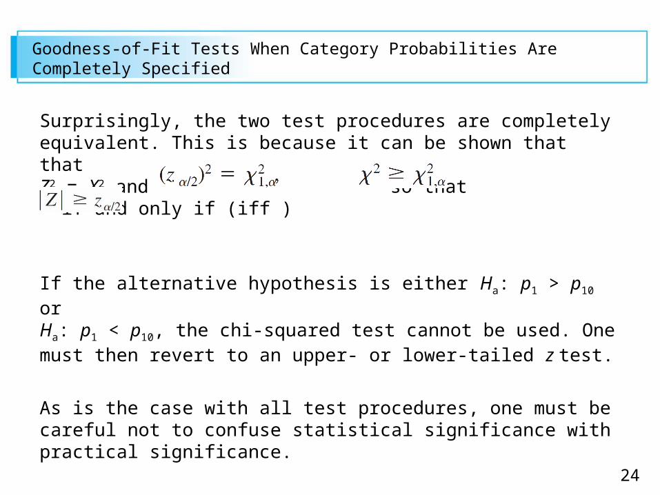
Surprisingly, the two test procedures are completely equivalent. This is because it can be shown that that Z2 = X2 and so that if and only if (iff )

If the alternative hypothesis is either Ha: p1 > p10 or Ha: p1 < p10, the chi-squared test cannot be used. One must then revert to an upper- or lower-tailed z test.

As is the case with all test procedures, one must be careful not to confuse statistical significance with practical significance.

25


A computed X2 that exceeds may be a result of a very large sample size rather than any practical differences between the hypothesized pi0’s and true pi’s.

Thus if p10 = p20 = p30 = , but the pi0’s true pi’s have

values .330, .340, and .330, a large value of X2 is sure to arise with a sufficiently large n.

Before rejecting H0, the s should be examined to see whether they suggest a model different from that of H0 from a practical point of view.

26

P-Values for Chi-Squared Tests

27


The chi-squared tests in this section are all upper-tailed, so we focus on this case.

Just as the P-value for an upper-tailed t test is the area under the tv curve to the right of the calculated t, the P-value for an upper-tailed chi-squared test is the area under the curve to the right of the calculated X2.

Appendix Table A.7 provides limited P-value information because only five upper-tail critical values are tabulated for each different .

28


The fact that t curves were all centered at zero allowed us to tabulate t-curve tail areas in a relatively compact way, with the left margin giving values ranging from 0.0 to 4.0 on the horizontal t scale and various columns displaying corresponding uppertail areas for various df’s.

The rightward movement of chi-squared curves as df increases necessitates a somewhat different type of tabulation.

The left margin of Appendix Table A.11 displays various upper-tail areas: .100, .095, .090, . . . , .005, and .001.

29


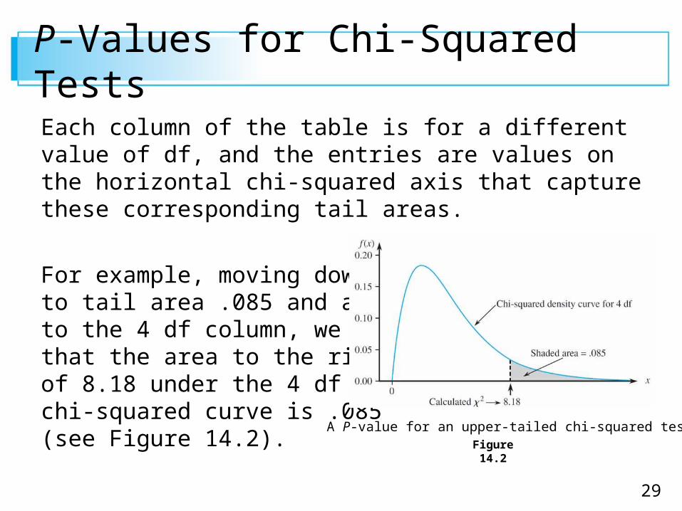
Each column of the table is for a different value of df, and the entries are values on the horizontal chi-squared axis that capture these corresponding tail areas.

For example, moving downto tail area .085 and acrossto the 4 df column, we seethat the area to the right of 8.18 under the 4 df chi-squared curve is .085(see Figure 14.2).

Figure 14.2

A P-value for an upper-tailed chi-squared test

30


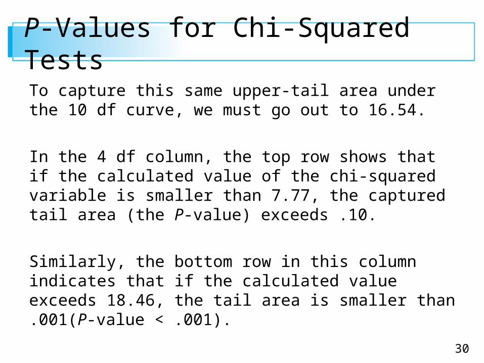
To capture this same upper-tail area under the 10 df curve, we must go out to 16.54.

In the 4 df column, the top row shows that if the calculated value of the chi-squared variable is smaller than 7.77, the captured tail area (the P-value) exceeds .10.

Similarly, the bottom row in this column indicates that if the calculated value exceeds 18.46, the tail area is smaller than .001(P-value < .001).

31

χ2 When the Pi’s AreFunctions of Other Parameters

32

χ2 When the Pi’s Are Functions of Other Parameters

Sometimes the pi’s are hypothesized to depend on a smaller number of parameters 1,…, m (m < k).

Then a specific hypothesis involving the i’s yields specific pi0’s, which are then used in the X2 test.

33

Example 2

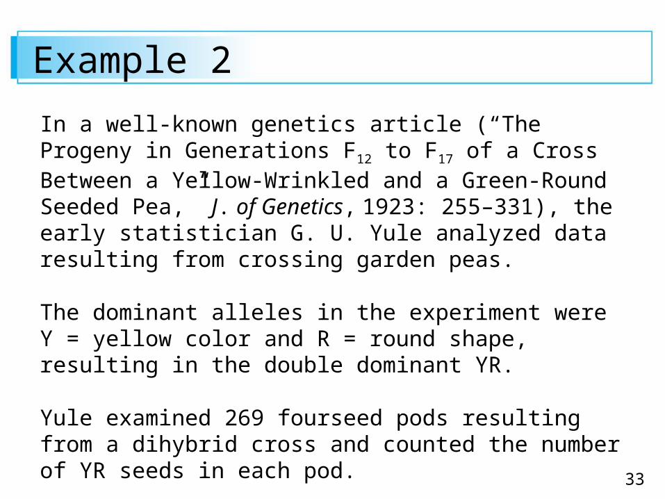
In a well-known genetics article (“The Progeny in Generations F12 to F17 of a Cross Between a Yellow-Wrinkled and a Green-Round Seeded Pea,” J. of Genetics, 1923: 255–331), the early statistician G. U. Yule analyzed data resulting from crossing garden peas.

The dominant alleles in the experiment were Y = yellow color and R = round shape, resulting in the double dominant YR.

Yule examined 269 fourseed pods resulting from a dihybrid cross and counted the number of YR seeds in each pod.

34

Example 2

Letting X denote the number of YRs in a randomly selected pod, possible X values are 0, 1, 2, 3, 4, which we identify with cells 1, 2, 3, 4, and 5 of a rectangular table (so, e.g., a pod with X = 4 yields an observed count in cell 5).

The hypothesis that the Mendelian laws are operative and

that genotypes of individual seeds within a pod are

independent of one another implies that X has a binomial

distribution with n = 4 and = .

We thus wish to test H0: p1 = p1 = p10 ,…, p5 = p50, where

pi0 = P(i – 1 YRs among 4 seeds when H0 is true)

cont’d

35

Example 2

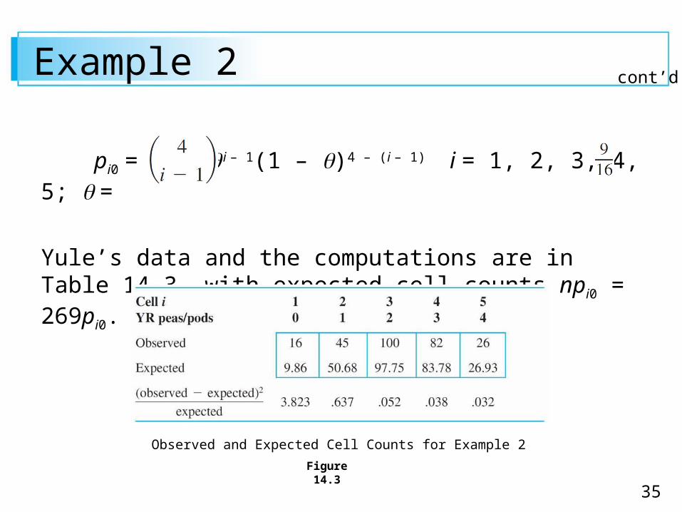
pi0 = i –

1(1 – )4 – (i – 1) i = 1, 2, 3, 4, 5; =

Yule’s data and the computations are in Table 14.3, with expected cell counts npi0 = 269pi0.

cont’d

Figure 14.3

Observed and Expected Cell Counts for Example 2

36

Example 2

Thus X2 = 3.823 + …. + .032 = 4.582.

Since = = 13.277, H0 is not rejected at level .01.

Appendix Table A.11 shows that because 4.582 < 7.77, the P-value for the test exceeds .10.

H0 should not be rejected at any reasonable significance level.

cont’d

37

χ2 When the Underlying Distribution Is Continuous

38


We have so far assumed that the k categories are naturally defined in the context of the experiment under consideration.

The X2 test can also be used to test whether a sample comes from a specific underlying continuous distribution.

Let X denote the variable being sampled and suppose the hypothesized pdf of X is f0(x).

39


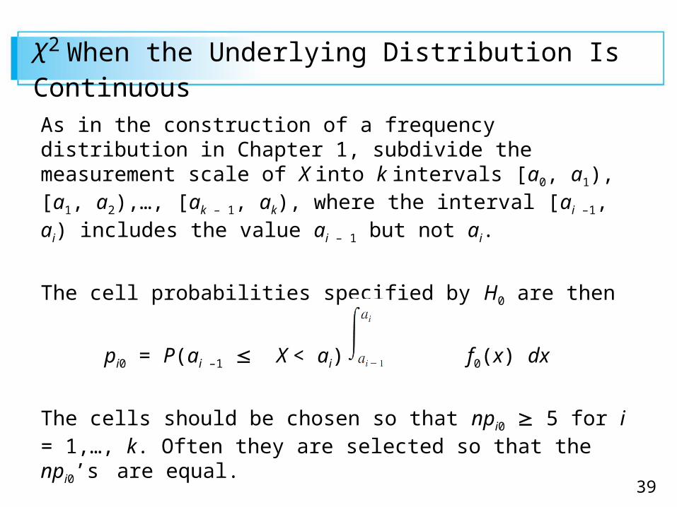
As in the construction of a frequency distribution in Chapter 1, subdivide the measurement scale of X into k intervals [a0, a1), [a1, a2),…, [ak – 1, ak), where the interval [ai –1, ai) includes the value ai – 1 but not ai.

The cell probabilities specified by H0 are then

pi0 = P(ai –1 X < ai) = f0(x) dx

The cells should be chosen so that npi0 5 for i = 1,…, k. Often they are selected so that the npi0’s are equal.

40

Example 3

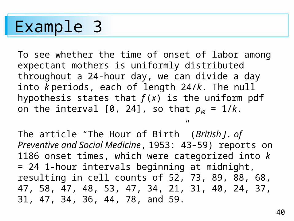
To see whether the time of onset of labor among expectant mothers is uniformly distributed throughout a 24-hour day, we can divide a day into k periods, each of length 24/k. The null hypothesis states that f (x) is the uniform pdf on the interval [0, 24], so that pi0 = 1/k.

The article “The Hour of Birth” (British J. of Preventive and Social Medicine, 1953: 43–59) reports on 1186 onset times, which were categorized into k = 24 1-hour intervals beginning at midnight, resulting in cell counts of 52, 73, 89, 88, 68, 47, 58, 47, 48, 53, 47, 34, 21, 31, 40, 24, 37, 31, 47, 34, 36, 44, 78, and 59.

41

Example 3

Each expected cell count is 1186 = 49.42, and the resulting value of X2 is 162.77.

Since = 41.637, the computed value is highly significant, and the null hypothesis is resoundingly rejected.

Generally speaking, it appears that labor is much more likely to commence very late at night than during normal waking hours.

cont’d

Documents

Copyright © Cengage Learning. All rights reserved. 14 Goodness-of-Fit Tests and Categorical Data Analysis