Copyright Warning & Restrictions

The copyright law of the United States (Title 17, United States Code) governs the making of photocopies or other

reproductions of copyrighted material.

Under certain conditions specified in the law, libraries and archives are authorized to furnish a photocopy or other

reproduction. One of these specified conditions is that the photocopy or reproduction is not to be “used for any

purpose other than private study, scholarship, or research.” If a, user makes a request for, or later uses, a photocopy or reproduction for purposes in excess of “fair use” that user

may be liable for copyright infringement,

This institution reserves the right to refuse to accept a copying order if, in its judgment, fulfillment of the order

would involve violation of copyright law.

Please Note: The author retains the copyright while the New Jersey Institute of Technology reserves the right to

distribute this thesis or dissertation

Printing note: If you do not wish to print this page, then select “Pages from: first page # to: last page #” on the print dialog screen

The Van Houten library has removed some of the personal information and all signatures from the approval page and biographical sketches of theses and dissertations in order to protect the identity of NJIT graduates and faculty.

ABSTRACT

Constitutive Equation for ConcreteUsing Strain-Space Plasticity Model

byYuxiang Xing

Plasticity theory has been used to model the concrete constitutive

relationship for about two decades. With the modifications and refinement based

on experimental data, achievement has been made in these plasticity models for

concrete. Almost all the existing models are developed in stress space. With a

lot of experimental data and more understanding about stress states of concrete,

the stress-space model shows many advantages. Because of this and also due

to conventional engineering practice, the stress-space plasticity approach has

been in the dominant position. However, the conventional stress-space plasticity

method has one inherent drawback in which it cannot deal with the softening

part of materials. To model effectively the descending part of the strain softening

materials such as concrete on the basis of plasticity theory, strain space concept

must be adopted. Some researcher used it as a supplemental means to the

stress-space model for the post-peak stage. Inspired by this basic idea, attempt

was made in this study, to set up a strain surface of concrete at critical stress,

then an initial yield surface and subsequent yield surfaces were constructed in

strain space according to the existing experimental results. A non-proportional

hardening rule and a non-associated flow rule were adopted. Finally, a strain-

space plasticity theory was presented in modeling the nonlinear multiaxial strain-

hardening-softening behavior of concrete.

It has been found that the model predictions of the ascending branch of

stress-strain behavior are in good agreement with the experimental results

involving a wide range of stress states and different types of concrete. The most

important inelastic behavior of concrete, such as brittle failure in tension; ductile

behavior in compression; hydrostatic sensitivities; and volumetric dilation under

compressive loadings are included in these comparisons. It has also been found

that the model can predict well the descending branch of strain-softening

behavior of concrete.

CONSTITUTIVE EQUATION FOR CONCRETEUSING STRAIN-SPACE PLASTICITY MODEL

byYuxiang Xing

A DissertationSubmitted to the Faculty of

New Jersey Institute of Technologyin Partial Fulfillment of the Requirements for the Degree of

Doctor of Philosophy

Department of Civil and Environmental Engineering

May 1993

Copyright @ 1993 by Yuxiang Xing

ALL RIGHTS RESERVED

APPROVAL PAGE

Constitutive Equation for ConcreteUsing Strain-Space Plasticity Model

Yuxiang Xing

Dr. C. T. Thomas Hsu, Thesis Advisor ( Date )Professor of Civil and Environmental Engineering, NJIT

Dr. George Weng, Committee Member ( Date )Professor of Mechanical and Aerospace Engineering, Rutgers University

Dr. M. Ala Saadeghvazinittee Member ( Date )Assistant Professor of Civil and Environmental Engineering, NJIT

Dr. D. Raghu, Commictee MembeY ( Date )Professor of Civil and Environmental Engineering, NJIT

Dr. W. R. Spillers, COmm- iftee Member ( Date )Professor and Chairman of Civil and Environmental Engineering, NJIT

BIOGRAPHICAL SKETCH

Author: Yuxiang Xing

Degree: Doctor of Philosophy in Civil Engineering

Date: May 1993

Undergraduate and Graduate Education:

• Doctor of Philosophy in Civil Engineering,New Jersey Institute of Technology, Newark, NJ, 1993

• Master of Science in Civil Engineering,Wuhan University of Technology, Wuhan, PR China, 1987

• Bachelor of Science in Civil Engineering,Wuhan University of Technology, Wuhan, PR China, 1982

Major: Civil Engineering

Publications:

Xing, Yuxiang, and Li, Gueiqing. " The Effect of Subjective Uncertainties onStructural Safety." Journal of Wuhan Institute of Urban Construction, No. 4,1987, (in Chinese).

Xing, Yuxiang, and Li, Gueiqing. An Experimental Study of R/C Frame withPartition Walls." Journal of Wuhan University of Technology, No. 2, 1988, (inChinese).

Xing, Yuxiang, and Li, Gueiqing. " Fuzzy Reliability of Seismic Structures."Journal of Wuhan University of Technology, No. 2 , 1990, (in Chinese).

Xing, Yuxiang, and Hsu, C. T. T. "Constitutive Equation for Concrete UsingStrain-Space Plasticity Model." Journal of Engrg. Mech., ASCE, (TentativelyAccepted).

iv

This thesis is dedicated tomy dear wife Lin Wang

V

ACKNOWLEDGMENT

The author wishes to express his sincere gratitude to his supervisor,

Professor C. T. Thomas Hsu, for his guidance, friendship and moral support

throughout this research.

Special thanks to Dr. G. Weng, Dr. M. A. Saadeghvaziri, Dr. D. Raghu

and Dr. W. R. Spillers for serving as members of the committee

Finally, the author expresses his gratitude to the Department of Civil and

Environmental Engineering and the Office of Graduate Studies for continuous

financial support in the pursuit of this degree.

vi

TABLE OF CONTENTS

Chapter Page

1 INTRODUCTION 1

1.1 General 1

1.2 Scope and Objective of Research 3

1.3 Statement of Originality 4

1.4 Structure of Thesis 6

2 CONSTITUTIVE MODELING OF CONCRETE 7

2.1 Introduction 7

2.2 Features of Concrete Behavior 7

2.3 Literature Review 16

2.3.1 Elasticity-Based Model 16

2.3.2 Plasticity-Based Model 17

2.3.3 Continuous-Damage Model .23

2.3.4 Plastic-Damage Model 23

2.3.5 Endochronic Theory 24

2.4 General Consideration of Strain-Space Plasticity Model 25

2.4.1 Advantages of Strain-Space Formulation 25

2.4.2 Current Status on Strain States of Concrete 28

2.4.3 Initial and Subsequent Yield Surfaces 31

2.4.4 Hardening and Softening Control 33

2.4.5 Non-Associated Flow Rule 33

3 STRAIN-SPACE CRITICAL SURFACE 37

vii

Chapter Page

3.1 Introduction 37

3.2 Strain-Space Critical Surface 37

3.2.1 General 37

3.2.2 Mathematical Preliminaries 39

3.2.3 General Properties of Critical Surface 40

3.2.4 Formulation of Critical Surface in Strain-Space Domain 42

3.3 Determination of Material Constants 45

3.4 Verification and Discussion of Formulated Surface 46

3.4.1 Comparison with Test Data of Kupfer et al (1969) 47

3.4.2 Comparison with Test Data of Schickert andWinkler (1977) 48

3.4.3 Comparison with Test Data of Nelissen (1972) 48

3.4.4 Strain State of High Hydrostatic Compression 49

4 PROPOSED CONSTITUTIVE EQUATION 53

4.1 Introduction 53

4.2 Yield Criterion 53

4.2.1 General Description 53

4.2.2 Formulation of Initial Yield Surface and SubsequentYield Surfaces 56

4.3 Hardening Rules 62

4.3.1 General 62

4.3.2 Modified Isotropic Hardening Rule 62

4.3.3 Effective Strain and Plastic Effective Stress 63

viii

Chapter Page

4.3.4 Effective Strain and Plastic Effective Stress Relation 66

4.3.5 Relationship between Hardening Parameter and PlasticModulus 66

4.3.6 Influence of Multiaxial Loading on Plastic Level 67

4.3.7 Kinematic Hardening Rule 72

4.4 Non-associated Flow Rule 74

4.5 Strain-Space Plasticity Formulation 76

4.6 Special Treatment on Post-Peak Behavior 78

4.6.1 Failure Modes 78

4.6.2 Stiffness Degradation in Strain Softening 79

5 MODEL PREDICTIONS 84

5.1 Introduction 84

5.2 Stiffness Matrix Co. / in Strain Softening 85

5.2.1 Degradation of Stiffness in Uniaxial Case 85

5.2.2 Stiffness Degradation Rate of Tensor C„ 86

5.3 Comparison Between Model Prediction and Experimental Results 87

5.3.1 Comparison with Kupfer's Test 87

5.3 .2 Comparison with Liu et al's Test 88

5.3.3 Comparison with Schickert and Winkler's Test 88

6 SUMMARY AND CONCLUSIONS 99

APPENDIX A DERIVATIVE OF LOADING FUNCTION ANDPLASTIC POTENTIAL 101

ix

Chapter Page

APPENDIX B FLOW CHART OF MATERIAL SUBROUTINE 105

REFERENCES 106

LIST OF TABLES

Table Page

2.1 Literature Review Chart for Plasticity Based Model 22

2.2 Little Is Known About Strain States Under Multiaxial Loadings 32

3.1 Basic Input for Kupfer et al's Critical Surface 47

3.2 Critical Surface Constant of Kupfer et al's 47

3.3 Basic Input for Schickert et al's Critical Surface 48

3.4 Critical Surface Constants of Schickert et al's 48

3.5 Basic Input for Nelissen's Critical Surface 49

3.6 Critical Surface Constants of Nelissen's 49

5.1 Basic Material Constants of Kupfer et al's Test 87

5.2 Basic Material Constants of Liu et al's Test 88

5.3 Basic Material Constants of Schickert and Winkler's Test 89

xi

LIST OF FIGURES

Figure Page

2.1 Uniaxial Tensile Test (Peterson (1981)) 8

2.2 Uniaxial Compressive Test 9

2.3 OSFP, OUFP and Ultimate Strength Envelopes for Concrete 13

2.4 Octahedral Normal Stress-Strain Relationship 14

2.5 Cyclic Uniaxial Compressive Stress-Strain Curve (Sinha (1964)) 15

2.6 Schematic Stress-Strain Relation for Concrete 15

2.7 Features of Softening Behavior 29

2.8 Loading Surfaces Defined in Stress and Strain Space 30

2.9 Yield Surface with Open End 34

2.10 Yield Surface with Closed End 34

2.11 Loading Surfaces of Modified Isotropic Hardening 35

2.12 Plastic Stress-Strain Relationship 36

3.1 Haigh-Westergaard Strain Space 41

3.2 The 0 ° and 60 ° Meridians from Existing Data 43

3.3 The 00 and 60 ° Meridians from Kotsovos and Newman 44

3.4 Geometry on the Deviatoric Plane 45

3.5 Test Points by Kupfer (1969) and Formula Prediction 50

3.6 Test Points by Schickert (1977) and Formula Prediction 51

3.7 Test Points by Nelissen (1972) and Formula Prediction 52

4.1 Results of Launay and Gachon's (1971) Study 54

4.2 Strain-Space Yield and Critical Surfaces 55

xii

Figure Page

4.3 Definition of ko 57

4.4 Relation Between k o ,k , and p i 59

4.5 Shape Function k = k ( p, ko ) 59

4.6 Relationship Between Failure Surface and Post-Peak Loading Surface 61

4.7 Relationship Between Elastic and Plastic Components 65

4.8 Plastic Work Increment 65

4.9 Normalized Stress-Strain Curves 68

4.10 Confined Uniaxial Compression Test by Palainsway and Shah (1974) 70

4.11 Plastic Stress-Strain Version of Palanisway and Shah's Data 70

4.12 Tensile Influence on M(ps ,0) 71

4.13 Hardening Rules 73

4.14 Stress and Strain Increments 82

4.15 incremental Plastic-Fracturing Energy 83

5.1 Comparison of Uniaxial Compressive Loading by Kupfer's Data 90

5.2 Comparison of Biaxial Compressive Loading by Kupfer's Data 90

5.3 Comparison of Biaxial Compressive Loading by Kupfer's Data 91

5.4 Comparison of Compression-Tension Loading by Kupfer's Data 91

5.5 Comparison of Compression-Tension Loading by Kupfer's Data 92

5.6 Comparison of Uniaxial Compressive Loading by Liu et al's Data 92

5.7 Comparison of Biaxial Compressive Loading by Liu et al's Data 93

5.8 Comparison of Biaxial Compressive Loading by Liu et al's Data 93

Figure Page

5.9 Comparison of Uniaxial Tensile Loading by Liu et al's Data 94

5.10 Comparison of Biaxial Tensile Loading by Liu et al's Data 94

5.11 Comparison of Biaxial Tensile Loading by Liu et al's Data 95

5.12 Comparison of Compression-Tension Loading by Liu et al's Data 95

5.13 Comparison of Compression-Tension Loading by Liu et al's Data 96

5.14 Comparison of Uniaxial Compressive Loading by Schickert's Data 96

5.15 Comparison of Nonproportional Loading by Schickert's Data (Path 1) 97

5.16 Comparison of Nonproportional Loading by Schickert's Data (Path 2) 97

5.17 Comparison of Nonproportional Loading by Schickert's Data (Path 3) 98

xi Hi

CHAPTER 1

INTRODUCTION

1.1 General

The rapid development of modern numerical analysis technique and high speed

digital computers have opened a new research field in concrete technology, that

is, the nonlinear numerical analysis of concrete structures. Such a structural

analysis is based on the fundamental principle of continuum mechanics, rather

than on empirical formulas.

In the past years, the methods of analysis and design for concrete

structures were mainly based on elastic analysis combined with various classical

procedures as well as on empirical formulas, using the results of a large amount

of experimental data. Such approaches are still necessary and continue to be

the most convenient for the ordinary design. However, the finite element method

now provides engineers with a powerful tool to explore possible new concept in

analysis and design. With the tool of finite element method, the tests can be

fewer in number and more fundamental, and consequently test results will be

more generally useful. The need for large-scale testing of members over the full

range of variables is greatly reduced.

The first attempt to apply the finite element method to a reinforced

concrete structure was made by Ngo and Scordelis (1967) in 1967. They

adopted the linear elastic-fracturing model for concrete in tension and bilinear

elastic-plastic model for reinforcement and for concrete in compression. Since

then, the importance of formulation of general constitutive equation for concrete

in finite element analysis has been well recognized, and a large variety of

models have been proposed for the stress-strain relation under short-term load,

2

based mainly on nonlinear elasticity, plasticity, continuous damage theory, and

endochronic theory of inelasticity, respectively.

Among these theories, plasticity theory, when not interpreted too

narrowly, is a most flexible model frame. In addition, it is rather simple. Thus it

has been a very active field.

In the classical plasticity, stress is treated as a basic quantity, and the

strain as a function of the stress. This form of stress-space plasticity is

consistent with human habit in stress-strain analysis. With a lot of experimental

data available, the stress-space plasticity theory has been in a dominant

position. On the basis of Drucker's postulates, it has been successfully used in

metals and other materials including concrete. However, it has one inherent

drawback that it cannot deal with softening part of materials.

in strain-space plasticity, on the other hand, strain is the basic quantity,

the stress is a function of the strain. By using ll'iushin's postulates, the strain

softening part as well as strain hardening part can be accounted in the same

way. Comparing with the stress-space counterpart, the strain-space plasticity is

much less used due to conventional engineering practice. This unbalanced

situation in concrete field was pointed out by Hsu (1972), and Bazant (1971).

Dougil I (1976), Bazant et al (1979), and Han et al (1986) had used the strain-

space plasticity concept for concrete constitutive law. They used it only as a kind

of supplemental ingredient to account for strain softening with very rough

approximations on loading surfaces. The significance of their research is that the

descending branch of stress-strain relation can be obtained using strain-space

approach. Since the yield and subsequent yield surfaces are not well

established for strain states of concrete, much improvement is needed. In

addition, to carry out the complete stress-strain behavior of concrete by strain-

space plasticity theory is a tremendous challenge. This is the motivation of the

3

present research. In this study, attempt was made to set up a strain surface of

concrete at the critical stress, then an initial yield surface and subsequent yield

surfaces were constructed according to the existing experimental results. A non-

proportional hardening rule and a non-associated flow rule were adopted.

Finally, a strain-space plasticity theory was presented in modeling the nonlinear

multiaxial strain-hardening-softening behavior of concrete. It is the belief that

with enough experimental data about strain states and more understanding of

strain behavior, the strain-space plasticity theory will become more powerful tool

to study the nonlinear behavior of concrete.

1.2 Scope and Objective of Research

The objective of this research work is to develop a short-term rate-independent

constitutive model for concrete, which can be used in finite element analysis of

concrete structures. The model is developed in the plasticity framework with

strain-space formulations. It is capable of predicting the stress-strain relation

with a reasonable accuracy. The stress states could be biaxial or triaxial tension,

mixed tension and compression, biaxial or triaxial compression. The most

important features of concrete behavior, including brittle cracking in tension,

strain-hardening and quasi-ductile behavior in compression, hydrostatic

sensitivities, nonlinear volumetric dilatancy and strain-softening, can be

represented by the constitutive model. This study will be performed mainly in the

following four aspects:

(1) To study the existing multiaxial experimental data, and analyze them

to reveal the strain characteristics of concrete under multiaxial

loadings.

4

(2) To define the initial yield surface, critical surface and subsequent

yield surfaces in a strain space.

(3) To formulate the strain-space plasticity in concrete, including

hardening rules, flow rule, and incremental stress-strain relationship.

(4) To compare the proposed model with the existing experimental

stress-strain results of concrete under multiaxial states of loadings.

Some of the important assumptions of the proposed model are stated

below:

(1) Concrete is considered macroscopically as isotropic and homogenous

material.

(2) Deformations are small enough to disregard the nonlinear terms of

the strain displacement relations.

(3) Elastic and plastic deformation are uncoupled in the strain hardening.

(4) The system is considered to be under isothermal conditions.

(5) The rate of loading is slow enough to disregard the inertia effects.

1.3 Statement of Originality

The concept of strain-space plasticity is relatively new and the followings may be

found original in this field of study:

(1) To select a critical surface in strain space.

In the conventional plasticity model for concrete, the initial yield

surface are defined according to the stress-space failure surface

which is known and available. By the same token, a reference surface

called critical surface is required in strain-space plasticity to define

the strain-space initial yield surface.

5

(2) To derive a closed initial yield surface in strain space.

For metals, the yield condition has a physical meaning and can be

determined by tests. However, the yield condition for concrete is a

fictitious quantity, and is usually defined according to the reference

surface. Many previous research defines the yield surface as reduced

size and same shape as the reference surface. Thus, the initial yield

surface from an open-ended failure surface has also got an open

end. It has been pointed out, however, that the initial yield surface in

stress space should be a closed shape. The strain-space initial yield

surface should also have an end along the hydrostatic pressure axis.

(3) To propose a non-proportional hardening rule.

The critical surface is one of the loading surface which has an open

end. During the change from the closed-ended initial yield surface to

the open-ended loading surfaces, the cross sectional shapes of the

surfaces on the deviatoric plane do not change, but their meridians

are varied. This means that high compression zone and low

compression or even tension zone have different strain hardening.

(4) To propose a non-associated flow rule.

The associated flow rule confines the plastic stress increment vector

normal to the loading surface, which implies no plastic volume

contraction occurs all the way in the plastic flow for certain loading

range. In addition, concrete has a large amount of volumetric

expansion after the critical stress. Therefore, the non-associated flow

rule must be used to define the ratio of the plastic stress components.

6

1.4 Structure of Thesis

Following this introductory chapter, Chapter 2 starts with the general features of

concrete behavior, which will help develop the proposed model. A review of the

constitutive modeling of concrete is made. Several modeling techniques are

briefly discussed. And a general consideration of the proposed model is

discussed.

Chapter 3 is devoted to analyzing the strain state of concrete under

multiaxial loadings and to setting up the strain-space critical surface.

Chapter 4 contains the proposed constitutive model based on strain-

space plasticity theory. This is followed by definitions of an initial yield surface

and subsequent yield surfaces, description of the non-proportional hardening

rule, explanation of the influence of hydrostatic pressure and lode angle,

adoption of the non-associated flow rule and special treatment for the strain

softening stage.

Chapter 5 contains model predictions and comparison with test results.

Finally, summary and conclusions are presented in Chapter 6.

CHAPTER 2

CONSTITUTIVE MODELING OF CONCRETE

2.1 Introduction

Characterization of stress-strain behavior of concrete has been a subject of

active research for a long time. A lot of constitutive models have been

developed. All these models have intrinsic advantages and disadvantages

dependent largely on their particular application. Before reviewing them, a brief

discussion on the features of concrete behavior is presented. In light of these

features, the merits and limitations of the reviewed models can be found. Based

on the literature review, a general consideration of the proposed model is

discussed, from which the basic thought of the proposed model can be seen and

the original concepts can be traced.

2.2 Features of Concrete Behavior

Concrete is a composite material. It consists of coarse aggregates and

continuous matrix of mortar which itself comprises a mixture of cement paste and

smaller aggregate particles. Its physical behavior is very complex, involving

phenomena such as inelasticity, cracking, creep, etc., being largely determined

by the structure of the composite material, such as the ratio of water to cement,

the ratio of cement to aggregate, the shape and size of aggregate, and the kind

of cement used. The following discussion is confined to the stress-strain

behavior of an average ordinary concrete. The structure of the material is

ignored and the rules of material behavior are developed on the basis of a

7

8

homogeneous continuum. Also the material is customarily assumed to be initially

isotropic.

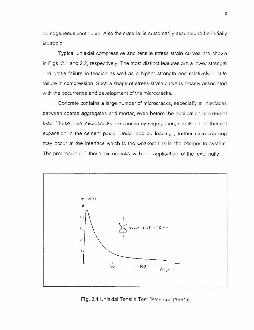
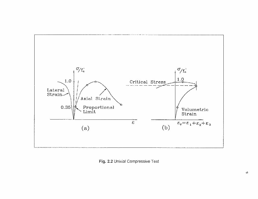
Typical uniaxial compressive and tensile stress-strain curves are shown

in Figs. 2.1 and 2.2, respectively. The most distinct features are a lower strength

and brittle failure in tension as well as a higher strength and relatively ductile

failure in compression. Such a shape of stress-strain curve is closely associated

with the occurrence and development of the microcracks.

Concrete contains a large number of microcracks, especially at interfaces

between coarse aggregates and mortar, even before the application of external

load. These initial microcracks are caused by segregation, shrinkage, or thermal

expansion in the cement paste. Under applied loading , further microcracking

may occur at the interface which is the weakest link in the composite system.

The progression of these microcracks with the application of the externally

c- (MPo)

---..--. gauge length : 40 TT

50 100(p.m)

Fig. 2.1 Uniaxial Tensile Test (Peterson (1981))

VolumetricStrain

Critical Stress

Fig. 2.2 Unixial Compressive Test

1 0

applied loads contributes to the generally obtained nonlinear stress-strain

behavior and plastic deformation of concrete.

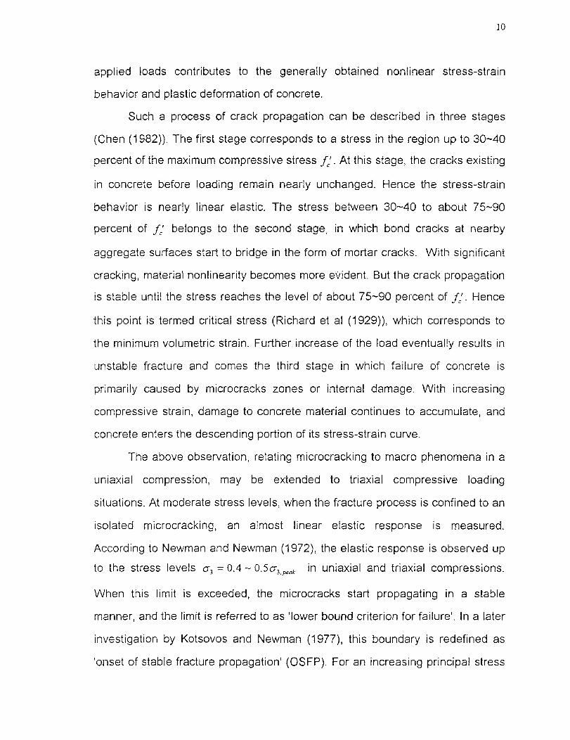
Such a process of crack propagation can be described in three stages

(Cheri (1982)). The first stage corresponds to a stress in the region up to 30-40

percent of the maximum compressive stress f;. At this stage, the cracks existing

in concrete before loading remain nearly unchanged. Hence the stress-strain

behavior is nearly linear elastic. The stress between 30-40 to about 75-90

percent of f; belongs to the second stage, in which bond cracks at nearby

aggregate surfaces start to bridge in the form of mortar cracks. With significant

cracking, material nonlinearity becomes more evident. But the crack propagation

is stable until the stress reaches the level of about 75-90 percent of f:. Hence

this point is termed critical stress (Richard et at (1929)), which corresponds to

the minimum volumetric strain. Further increase of the load eventually results in

unstable fracture and comes the third stage in which failure of concrete is

primarily caused by microcracks zones or internal damage. With increasing

compressive strain, damage to concrete material continues to accumulate, and

concrete enters the descending portion of its stress-strain curve.

The above observation, relating microcracking to macro phenomena in a

uniaxial compression, may be extended to triaxial compressive loading

situations. At moderate stress levels, when the fracture process is confined to an

isolated microcracking, an almost linear elastic response is measured.

According to Newman and Newman (1972), the elastic response is observed up

to the stress levels 0 -3 = 0.4 — 0.50-3 peak in uniaxial and triaxial compressions.

When this limit is exceeded, the microcracks start propagating in a stable

manner, and the limit is referred to as 'lower bound criterion for failure'. In a later

investigation by Kotsovos and Newman (1977), this boundary is redefined as

'onset of stable fracture propagation' (OSFP). For an increasing principal stress

II

a., eventually the above mentioned minimum volume can be obtained. Newman

and Newman (1972) refer to this boundary as 'upper bound criterion for failure',

and later Kotsovos and Newman term this boundary as 'onset of unstable

fracture propagation' (OUFP). Upon further increasing stress, beyond OUFP, a

maximum stress level is reached. When proper measures are taken, the fracture

process also remains stable beyond peak stress, and a descending branch is

obtained. When the hydrostatic pressure is very large, the concrete may get

crushed at the maximum stress level. Thus, no strain softening follows.

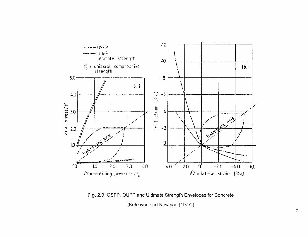
In Fig. 2.3(a), the above mentioned stages in the progressive fracture

process are shown in the meridian plane in principal stress space. The meridian

plane contains all loading combinations that can be investigated with standard

triaxial cylinder tests. In Fig. 2.3(b), the strain-space counterparts are plotted.

Fig. 2.3 show that the OSFP curve is closed, while the OUFP envelope and

ultimate strength envelope are open ended with regard to the hydrostatic axis.

According to Kotsovos and Newman (1977), the OSFP-envelope is associated

with the fatigue strength of the concrete. Below this level, concrete does not

suffer from any significant cracking. The OUFP-level is associated with the long-

term strength of the material.

Concrete is a dilatant material. As illustrated in Fig. 2.2(b), the change in

volume is almost linear up to the critical stress. At the point of critical stress,

however, the direction of volume change is reversed, resulting in a volumetric

expansion. For the multiaxial cases (Kupfer and Gerstle (1973)), the volumetric

strain against the octahedral stress is shown in Fig. 2.4. Before the point of

critical stress, the volumetric strain decreases. After the critical stress, however,

the tendency is reversed with increasing stress. The volume expansion near

failure is due mainly to the voids within the body which are caused by the crack

propagation.

12

In the tension case, as the tension state of stress tends to arrest the

cracks much less frequently than the compressive state of stress, the interval of

stable crack propagation is quite short. Then starts the unstable crack

propagation. That is why the deformation behavior in tension is quite brittle. In

addition, the aggregation-mortar interface has a significantly lower tensile

strength than that of the mortar. This is why the concrete material has a very low

tensile strength. Under uniaxial tension, the stress-strain diagram is linear or

nearly linear up to failure stress (Kupfer et at (1969) , Carino et al (1976)). As for

the biaxial tension and triaxial tension, it is reported (Ahmed (1981)) that the

behavior is similar to that under uniaxial tension and the tensile strength is

almost the same as the one under uniaxial tension.

The occurrence of microcracking and slip also leads to softening

degradation of the stiffness. Fig. 2.5 (Sinha et el (1964)) illustrates a typical

stress-strain curve of concrete under compressive cyclic loading. The envelope

curve has a descending part beyond the ultimate stress, and the unloading-

reloading curves are not straight-line segments but loops of changing size with

decreasing average slopes. Assuming that the average slope is the slope of a

straight line connecting the turning points of one cycle and that the material

behavior upon unloading and reloading is linearly elastic (dotted line in the

figure). Then the elastic modulus degrades with increasing straining. For the

descending part, a significant degradation of stiffness can be observed.

In summary, concrete is a material which has higher strength and larger

ductility in compression than those in tension; it has a significant volumetric

expansion after the point of critical stress, and also a significant amount of

irrecoverable strain during unloading. In general, the stress-strain curve

experiences an elastic-plastic-hardening-softening process under monotonically

compressive loading.

-12- OSFP—•-- OUFP ultimate strength

f' uniaxial compressivestrength

5.0

(a.)

4. 0

-10(b.)

7Cro

ru

-

r

rm' 3.0wL.

2.0

IP*

•//

1D

-111211=100.0.26..."421 -Ur-

() 1.0 2.0 3.0 4D

/2 x confining pressure / f c'

4.0 2.0 0 -2.0 -4.0 -6.0/2 x lateral strain Woe)

J

Fig. 2.3 OSFP, OUFP and Ultimate Strength Envelopes for Concrete

(Kotsovos and Newman (1977))

(Concrete 2)i tcu • 324 kp/crrii Ko 556

Test results

---Calculation results

14

Fig. 2.4 Octahedral Normal Stress-Strain Relationship

(Kupfer and Gerstle (1973))

.001 .002 .003 .004 .005 .006 .007

Compression (—)

Tension

BrittleCracking

PerfectHardening Plasticity

_ _ Ductile

Softening

Crushing

Fig. 2.5 Cyclic Uniaxial Compressive Stress-Strain Curve (Sinha (1964))

15

Fig. 2.6 Schematic Stress-Strain Relation for Concrete

16

2.3 Literature Review

In recent years, a large variety of analytical models have been proposed to

characterize the short-term, rate-independent stress-strain behavior of concrete

materials. The existing approaches can be categorized as nonlinear elasticity

theory, plasticity theory, continuous damage theory, and endochronic theory.

Here only the basic ideas are reviewed.

2.3.1 Elasticity -Based Model

The nonlinear elasticity models assume that the nonlinear behavior of concrete

can be represented by appropriately changing the tangent modulus (for

incremental formulation of hypoelastic type) or changing the secant modulus (for

total stress-strain formulation of Cauchy type and hyperelastic type). Among

many propositions, the nonlinear incrementally orthotropic models (Darwin et al

(1974), Liu et al (1972)) are based on the equivalent uniaxial stress-strain

relationships. Different forms of material functions have been proposed to make

the model more flexible in curve-fitting of the biaxial test data. The limiting state

of the nonlinear elastic model is usually defined by a biaxial stress failure

envelope. These nonlinear models can be applied to biaxial loading only. They

give no information on the value of the third normal strain component. For triaxial

analysis, the nonlinear elastic isotropic models have been proposed (Kupfer et

al (1973) ,Cedolin et al (1977), Kotsovos et al (1978)). These models use

stress(strain) dependent secant or tangent bulk and shear modulus. Based on

experimental results, a consistent octahedral stress-strain relationship can be

written for all states of stress, and a generalized bulk modulus and a generalized

shear modulus can be used as the nonlinear material coefficients. Following the

similar concept, Ottosen (1979) proposed a more general form of triaxial stress-

17

strain relation. In his model, a sophisticated failure surface (Ottosen (1977)) is

used as the limiting surface, and a stress point inside this surface is mapped to a

nonlinearity index. This index in turn corresponds to a secant elastic modulus.

To simulate the volume expansion, the model allows the secant value of

Poisson's ratio to increase proportionally if the index is larger than certain value.

In a similar way, Ottosen's model even can handle the softening behavior

(Ottosen (1982)).

In general, nonlinear elasticity models are simple to use, and usually can

generate stress-strain response accurately if a broad data base is available.

However, its applicability is restricted to a particular type of stress condition.

Usually the material functions are directly determined from a curve-fitting

procedure. There can be no guarantee of general usefulness outside the range

that is covered by the data on which the rules are based. Moreover, this

approach can not include the residual strain, and thus the unloading can not be

considered. This greatly restricts the application of the approach from the

fundamental point of view. Since even for a monotonic loading condition, local

unloading often occurs during the progressive yielding and fracture of the

concrete.

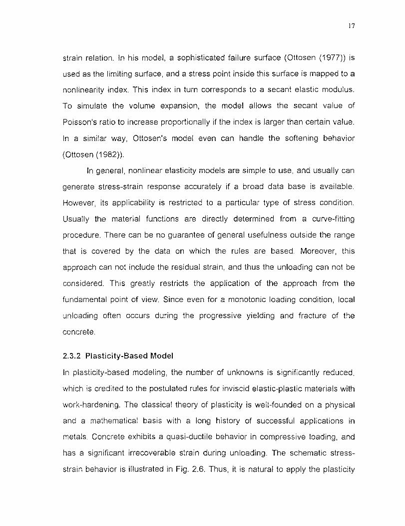
2.3.2 Plasticity -Based Model

In plasticity-based modeling, the number of unknowns is significantly reduced,

which is credited to the postulated rules for inviscid elastic-plastic materials with

work-hardening. The classical theory of plasticity is well-founded on a physical

and a mathematical basis with a long history of successful applications in

metals. Concrete exhibits a quasi-ductile behavior in compressive loading, and

has a significant irrecoverable strain during unloading. The schematic stress-

strain behavior is illustrated in Fig. 2.6. Thus, it is natural to apply the plasticity

18

theory to concrete. Suidan and Schonobrich (1973) first used this theory in

concrete. In their work, the von Mises yielding criterion was used with

augmentation of a tension-cut-off surface to account for the low tensile capacity

of concrete. Following the similar idea, Drucker-Prager criterion and Mohr-

Coloumb criterion were used with augmentation of tension-cut-off in many

computer programs for concrete structural analysis (Argyris et al (1974), (1976)).

Later it was recognized that these criteria predicted a much higher strength

value than the experimental data. This was due to the fact that the straight

meridians were used in the yield surfaces. Chen and Chen (1975) and

Buyukorturk (1977) considered separate yield criteria for compression zone and

tension zone, respectively, and used the curved meridians, which predicted the

biaxial failure envelope with good accuracy. With more experimental

investigations reported, the shape of failure surface became more and more

clear. And the mathematical representations of failure functions were obtained (

Hsieh, Ting, and Chen (1982), Wiliam and Warnke (1974), and Ottosen (1977)).

They are generally accepted failure surfaces. As soon as the failure function has

been chosen, the yield function is usually assumed to have the same form but

reduced in size. Thus, the constitutive relation can be formulated by the

conventional approach that is used in metal.

The essential elements of any model based on classical plasticity theory

are the yield criterion, the flow rule and the hardening rule. Because concrete is

not an ideal elastic-plastic material, modifications and refinement must be

made. To this end, much work around the above three aspects was done, such

as the work by Han and Chen (1985). They used the non-proportional hardening

rule and close-ended initial yield surface to solve the problem that previous

models overestimated the plastic tensile strain for tensile loading and

underestimated the compressive strain for confined compressive loading.

19

Torrent et al (1987) solved it through a different approach. Buyukorturk (1979)

improved the volume expansion after the critical stress by using the non-

associated flow rule and a dilantancy factor, which was a function of the

hardening parameter.

The use of plasticity models of concrete behavior has many advantages.

It accounts for the history-dependent behavior. Residual strain due to unloading

can be evaluated. It allows unloading and reloading, thus provides rooms for

modeling cyclic loading problems. However, one tremendous disadvantage for

this model is that the strain softening behavior can not be evaluated in the

traditional stress-space plasticity methods. This is because the softening

behavior is a history of strain rather than stress. In the compression test, a

complete stress-strain curve including the descending part can only be obtained

under strain control condition. In this sense, the strain-space plasticity methods

is needed for the studying of strain softening materials.

The possibility of formulating plasticity theory in strain-space was

recognized by Drucker (1950). However, the details of a strain-space formulation

were not completed. A strain space formulation of plasticity was first presented

by ll'iushin (1961). Nevertheless, Il'iushin's work was not aimed at developing a

new approach to the theory of plasticity, but rather to introduce a general

plasticity postulate, which is less restrictive than Drucker's postulates, and has

the advantage to treat simultaneously stable and unstable behavior of the

materials. It is by Naghdi and Trapp (1975) and Casey and Naghdi (1981,1983a)

that the significance of a strain-space formulation of plasticity is recognized. In

their studies, new criteria for plastic loading were presented that were of general

validity including the case of softening materials.

Meanwhile, Dougill (1976) adopted the strain-space formulation in

developing an ideal material (the so-called progressively fracturing solid model).

20

He suggested a way in which a continuum theory may be devised to describe

the effects of stable progressive fracture in a heterogeneous solid. Dafalias

(1977a, b) examined the thermodynamic aspects of the work of ll'iushin, and he

presented formulations which, for isothermal conditions, were similar to the ones

presented by Naghdi and his coworkers. A different approach in the context of

strain-space plasticity was followed by Yoder and Iwan (1981), who introduced a

relaxed stress as an equivalent notion of the plastic strain. And they claimed that

the stress-space and strain-space formulations of plasticity were equivalent.

Although this conclusion does not hold according to Casey and Naghdi (1983b),

it has been shown that many of the familiar features of stress-space plasticity

can be carried over to the strain-space plasticity.

The attempt of strain-space plasticity in concrete was made by Bazant

and Kim (1979). In their work, a Drucker-Prager formulation in strain space was

adopted as the fracturing surface. Inspired by Bazant and Kim's work, Han and

Chen (1986) discussed in details the strain-space plasticity formulas

incorporating the fracture contribution to the loading surface. In their study, the

loads before the peak load used the conventional stress-space loading surfaces.

After the peak load, the stress-space loading surfaces were replaced by the

strain-space loading surfaces for the descending part. The feature of volume

dilatancy was used as a loading condition and the loading surfaces actually

were the planes parallel to the ir plane. The shift from stress-space to strain-

space at the peak point was good, but the simple loading surfaces for the

softening part lost much information of deviatoric component. Further study in

this aspect is needed.

Recently, there appeared two papers in the field of the strain-space

plasticity-based approach. They introduced the loading surfaces in strain-space

in different ways. Mizuno and Shigemitsu (1992) selected three-parameter Lade

21

type load function in stress space as a basis and derived the strain-space

loading function by the method proposed by Naghdi and Trapp (1975). The

loading parameter was defined directly as a function of plastic work through the

tests of their own. Their model was developed to discuss the confined uniaxial

loading case. For a general 3D situation, it inherits two problems: a) The initial

loading surface is not closed along the negative hydrostatic axis. b) The relation

between the loading parameter and plastic work is too difficult to obtain for

general usefulness.

Pekau et al (1992) defined the peak strength state as an initial failure

state and the fracture point state as a final failure state. They constructed the

initial yield surface and initial failure surface using the test data of Kotsovos

(1979). The final failure surface was assumed as an outward isotropic expansion

surface with respect to the initial failure surface. They used the concept of

closed initial yield surface. The contribution was no doubt by using a closed

initial yield surface and the attempt to set up the surfaces in strain space directly

through the experimental data. However, there are some problems: a) The strain

state is too sensitive to the test environment. Thus, an accurate strain

measurement in the multiaxial case is extremely hard to obtain at failure (Gerstle

(1980)). It has been found that the existing data of strain state at ultimate

strength are very scattered. Therefore, it is unsuitable for or not reliable to

setting up a surface based on these test data at failure state. b) The loading

surface can not be all closed according to the test results by Kotsovos (1979). c)

Only an associated flow rule was used, which implies underestimating the plastic

volume contraction. d) The assumed initial yield surface had little relation with

the defined failure surface. This may result in an inconsistency in the constitutive

equation for tension, and tension-compression regions.

Table 2.1 Literature Review Chart for Plasticity Based Model

Stress-Space Plasticity Strain -Space Plasticity

Classical Theory of Plasticity for Metals Basic Theory of Strain-Space PlasticityPrager

Drucker'sConsistencyA Unified

Loading-Unloading(1949): Loading Function,

Criteria

Postulates (1951):Condition,

Method

Drucker (1950): Possibility ofStrain-space Formulation

lliushin's Postulates(1961):Basis of Strain-Space For-mutation, Less Restrictions

Dafalias (1977): FurtherProof and Development

Naghdi et al (1975): Strain-space Formulation, Signific-ance, And Comparison withStress-space Formulation

Dougill (1976): Special For-mulation (Stiffness Degrad-ation Included), SpecialLoading Surface and Hard-ening Relation

Yoder and Iwan (1981):Stress Relaxation Concept,Von Mise Form LoadingSurfaces in Strain Space

In ConcreteBazant and Kim (1979):First Use Strain-space Plasticityto Concrete. Drucker-PragerForm in Strain Space

Han and Chen (1986): Gen-eral Formulation, Volume •Expansion as Loading Crit-eron for Strain Softening

Mizuno et al (1992): Use Naghdi'sMethod on Lade TypeSurface, Confined Uniaxial Case

Pekau et al (1992): DefineStrain Surface at Failure,From Existing Data

Suidan and Schonobrich (1973):Introduce Plasticity to ConcreteVon Mises Yield Surface withTension-cut-off Cap for Tension

Chen and Chen (1975):Buyukorturk (1977):Separate Yield Criteria for Com-pression and Tension, CurvedMeridian Loading Surfaces

Buyukorturk (1979): Non-associa-ted Flow Rule, Dilatancy Factor

Han (1985), Torrental (1987):Closed Yield Surface, Non-proportional Hardening Rule

23

In summary, one more inherent disadvantage of these two recent

constitutive models just mentioned is that too many parameters are needed to

define the constitutive equation, thus the model are too complicated.

Table 2.1 shows a review chart for the plasticity-based model.

2.3.3 Continuous -Damage Model

Continuous damage mechanics was introduced by Kachanov (1958). He used

the effective stress concept to model the creep rupture of metals. The effective

stress concept has been applied to concrete by Krajcinovic (1979), Loland

(1980), and Mazars (1981). Continuous damage mechanics is concerned with

the description of progressive weakening of solids due to the development of

microcracks and microvoids. The microcracking destroys the bond between

material grains, affects the elastic properties, and may also result in permanent

deformation. Many damage models were proposed (Krajcinovic et al (1981),

Krajcinovic et al (1985), Ortiz (1985), Simo and Ju (1985), and Resende (1987)).

A general continuous damage model has three essential parts: a set of

independent internal variables, a set of equations of the stress to the strain and

the internal variables, and a set of flow rules specifying the way in which the

internal variables increase when loading proceeds. It has been realized that

there are several facets of concrete behavior that cannot be represented by this

type of model, most of all is the plastic flow caused by slip process.

2.3.4 Plastic - Damage Model

Since both microcracking and plastic flow are present in the nonlinear response

of concrete, a constitutive model should address equally the two physically

distinct modes of irreversible damages and should satisfy the basic postulates of

mechanics and thermodynamics. The plastic-damage theory gives a unified

24

approach to the modeling of concrete. It was first proposed by Dragon and Mroz

(1979), and Bazant and Kim (1979). This type of model generally has the

advantages of both plasticity model and continuous damage model.

Within the general formulation of plastic-damage theory, two surfaces are

established, a plasticity surface and a damage surface. This is accomplished by

using the second law of thermodynamics, expressed in the form of the internal

dissipation inequality. The two surfaces are then invoked simultaneously to

obtain the increments of plastic strain and an additional strain due to damage.

Sometimes, only one surface is used as a loading surface from which the sum of

contributions of microcracking and plastic flow can be induced with the

introduction of damage parameter into classical plasticity. This is why the

plastic-damage theory (or plastic-fracturing theory) is generally considered in the

category of plasticity. Recently, a lot of work were done in this field (Han and

Chen (1986), Lubliner et al (1989), Frantziskonis et al (1987), and Yazdani et al

(1990)). With the improvement of both plasticity method and damage approach,

the new version of plasticity-damage model can be developed along the general

line.

2.3.5 Endochronic Theory

The endochronic theory was originally proposed by Valanis (1971) in

viscoelasticity and was first applied to concrete by Bazant et al (1976). It uses a

strain-increment-dependent non-decreasing scalar variable, called intrinsic time

to represent the evolution of the increase of irreversible damage from which the

inelastic strain can be obtained. The intrinsic time measured is comparable to

that of the effective plastic strain measured in plasticity theory. The theory does

not require specific definitions of yielding or hardening. The inelastic strains are

related to the intrinsic time through a series of mappings. The mapping functions

25

also depend on the current state of stress and strain and are determined from

the experimental data. Consequently, the model is incrementally nonlinear. This

type of model can cover many phenomena like nonlinear behavior, inelastic

volume dilatancy, hydrostatic pressure sensitivity and strain-softening, etc.

However, these can be achieved only at the expense of greater complexity and

increasing number of material parameters, and the model involves many

functions which are computed by a complicated optimal-fitting procedure.

Besides , the incremental nonlinearity of the stress-strain relation is inconvenient

for numerical structural analysis, which requires iterations within each increment

of loading.

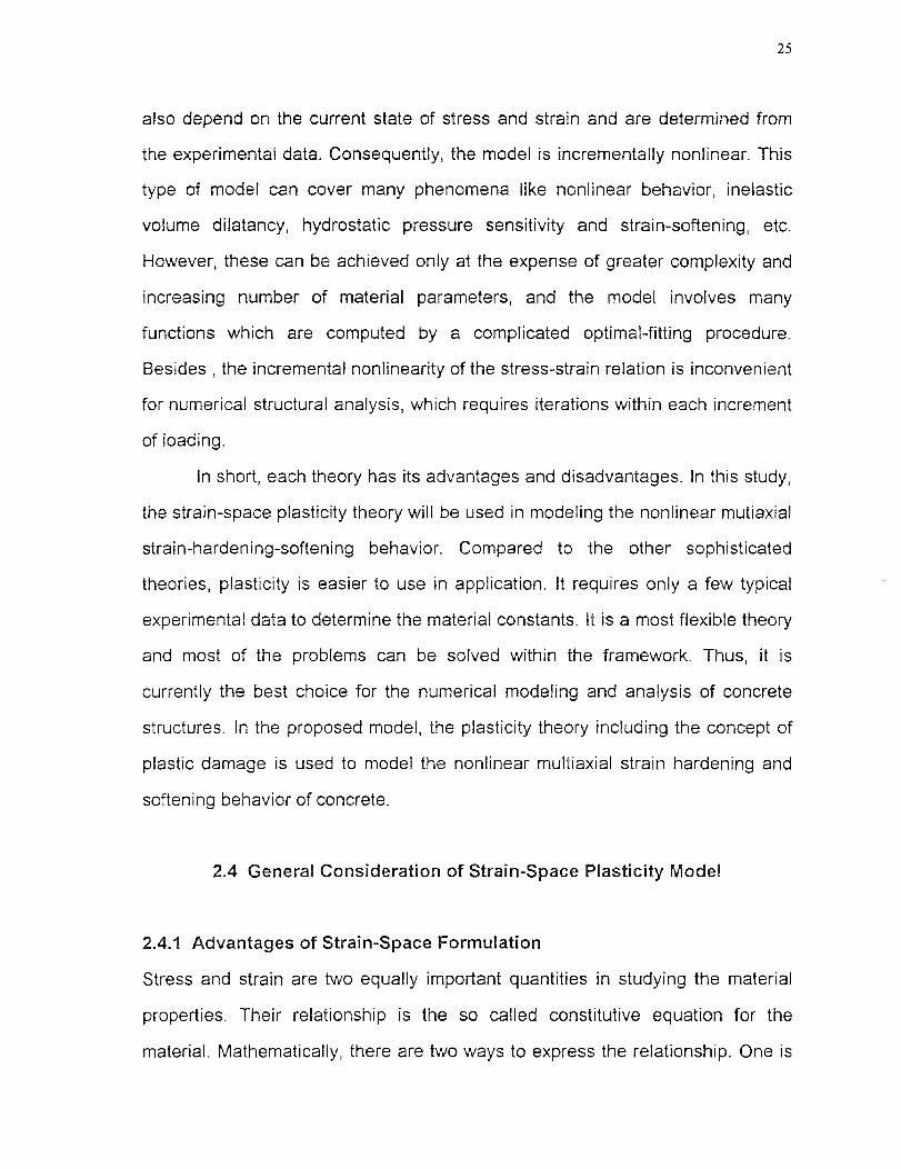
In short, each theory has its advantages and disadvantages. In this study,

the strain-space plasticity theory will be used in modeling the nonlinear mutiaxial

strain-hardening-softening behavior. Compared to the other sophisticated

theories, plasticity is easier to use in application. It requires only a few typical

experimental data to determine the material constants. It is a most flexible theory

and most of the problems can be solved within the framework. Thus, it is

currently the best choice for the numerical modeling and analysis of concrete

structures. In the proposed model, the plasticity theory including the concept of

plastic damage is used to model the nonlinear multiaxial strain hardening and

softening behavior of concrete.

2.4 General Consideration of Strain-Space Plasticity Model

2.4.1 Advantages of Strain -Space Formulation

Stress and strain are two equally important quantities in studying the material

properties. Their relationship is the so called constitutive equation for the

material. Mathematically, there are two ways to express the relationship. One is

26

to use stress as basic variable and stress as function. The equation obtained is

called stress-space formulation. The other is to use strain as basic input and

stress as function. This later form is the strain-space formulation.

For the linear stage of material, Hooke's law is used, hence, one

formulation can be derived from the other. They are equivalent. However, when

material gets into nonlinear stage, especially when the material enters into

strain softening region, these two versions do have some differences.

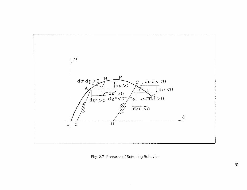
Consider a typical uniaxial stress-strain curve shown in Fig. 2.7. The

material behavior is said to be stable along the ascending (hardening) part OP

of the curve, and unstable along the descending (softening) part PQ. The feature

of unstable behavior is that as the strain increases, the stress decreases,

otherwise the material would accelerate to failure if the stress keeps constant.

On the other hand, if the strain is decreased instead of increased at a point C in

the descending part, the stress still decreases but now along an elastic

unloading line CH. Reloading would trace back the unloading line until the yield

stress at point C is reached. Such a complete stress-strain curve including the

descending (softening) part can only be obtained from a test under strain control

condition. Therefore, softening is a history of strain rather than stress which

must be determined from the equilibrium at all times.

This one-dimensional unstable behavior is generalized to a multiaxial

state of stress and strain in a similar manner to that of stable material. In stress

space, a state of stress is represented by a point, as can be seen in Fig. 2.8(a).

If a point A is on the loading surface f = 0 and the material is stable, a stress

increment do- must be directed outward in order to induce a plastic as well as

elastic increment of strain, otherwise an increment directed inward would cause

elastic strain only. The outward motion of the stress point, which carries the yield

surface along with it, corresponds to a hardening stress-strain curve for

27

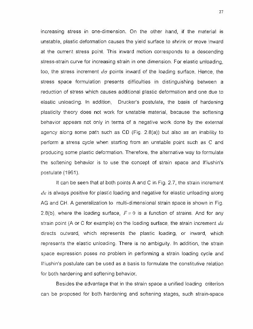
increasing stress in one-dimension. On the other hand, if the material is

unstable, plastic deformation causes the yield surface to shrink or move inward

at the current stress point. This inward motion corresponds to a descending

stress-strain curve for increasing strain in one dimension. For elastic unloading,

too, the stress increment do- points inward of the loading surface. Hence, the

stress space formulation presents difficulties in distinguishing between a

reduction of stress which causes additional plastic deformation and one due to

elastic unloading. In addition, Drucker's postulate, the basis of hardening

plasticity theory does not work for unstable material, because the softening

behavior appears not only in terms of a negative work done by the external

agency along some path such as CD (Fig. 2.8(a)) but also as an inability to

perform a stress cycle when starting from an unstable point such as C and

producing some plastic deformation. Therefore, the alternative way to formulate

the softening behavior is to use the concept of strain space and Il'iushin's

postulate (1961).

It can be seen that at both points A and C in Fig. 2.7, the strain increment

dE is always positive for plastic loading and negative for elastic unloading along

AG and CH. A generalization to multi-dimensional strain space is shown in Fig.

2.8(b), where the loading surface, F =0 is a function of strains. And for any

strain point (A or C for example) on the loading surface, the strain increment de

directs outward, which represents the plastic loading, or inward, which

represents the elastic unloading. There is no ambiguity. In addition, the strain

space expression poses no problem in performing a strain loading cycle and

ll'iushin's postulate can be used as a basis to formulate the constitutive relation

for both hardening and softening behavior.

Besides the advantage that in the strain space a unified loading criterion

can be proposed for both hardening and softening stages, such strain-space

28

formulation of plasticity also has following positive features: (1) The

displacement method in finite element analysis of nonlinear structures is

consistent with material expression in strain space. In the iteration process, the

stresses do not need to be computed unless they are specifically desired. (2)

For the method of variable stiffness iteration, the iterations can be performed in

both the hardening and softening stages when strain is used as the variable. (3)

When the stiffness matrix is formed at the midpoint value of strain or stress of

the preceding load step, the results in strain space are better, particular in the

region near the ultimate strength. A good and clear statement of the advantages

about the strain-space plasticity can be found in Naghdi et al (1975) and Yoder

et al (1981).

Having above attractive merits, in this study, the strain-space plasticity

theory is chosen as the basis to set up a relatively comprehensive model to

describe the behavior of concrete including both strain hardening and strain

softening. For metals and other materials with the same properties in

compression and tension, the application of the strain-space plasticity method

has been successfully proved. Its use in concrete is relatively new. The pioneer

work of Bazant et at (1979) and Han et al (1986) showed the promising and

feasibility in comprehensive and further research.

2.4.2 Current Status on Strain States of Concrete

Although the strain-space formulation has the above advantages, it has one

tremendous disadvantage that very few test data are available for the strain

states of concrete. Thus relatively less is known about the strain states behavior

under multiaxial loadings, which makes it difficult to set up loading surfaces of

the strain-space plasticity theory. In multiaxial space, whether in stress space or

in strain space, a surface is used to define the state of a material. For example,

do- de <0

dEP >0

do- <0

>0

Pdo- de >0

do- >0A 44---de >0

der' >0 dEe <C)

Fig. 2.7 Features of Softening Behavior

Hardening Loadingdf>0

Hardening LoadingB dF>0

30

(a) In Stress Space

(b) In Strain Space

Fig. 2.8 Loading Surfaces Defined in Stress and Strain Space

31

a failure surface in stress space defines the ultimate strength for any ratio of

stresses. Table 2.2 gives the information about the important states of concrete

in both stress space and strain space. It shows that in stress space, the function

of failure surface is considered known and it has actually been used widely,

while in strain space, little is known. Although many researches have been done

in this aspect, the results are far from satisfactory. To completely and accurately

analyze the strain states of concrete, a compressive experimental research is

needed with strain-controlled testing methods. Almost all the existing multiaxial

test data are obtained from the stress-controlled tests. At present situation, a

good attempt may be made to quantitatively analyze the strain states by

extracting information from the existing data together with appropriate

assumptions. Then check and verify the derived equations with the test data.

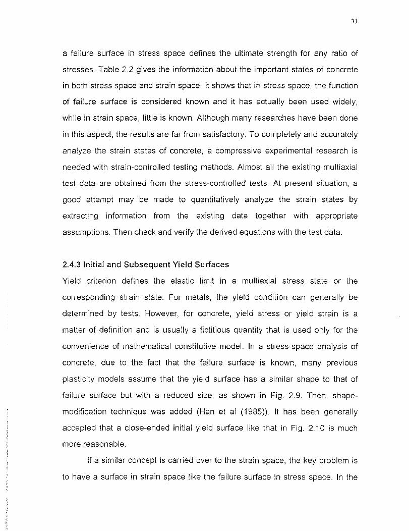
2.4.3 Initial and Subsequent Yield Surfaces

Yield criterion defines the elastic limit in a multiaxial stress state or the

corresponding strain state. For metals, the yield condition can generally be

determined by tests. However, for concrete, yield stress or yield strain is a

matter of definition and is usually a fictitious quantity that is used only for the

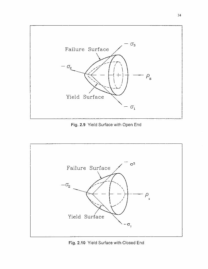
convenience of mathematical constitutive model. In a stress-space analysis of

concrete, due to the fact that the failure surface is known, many previous

plasticity models assume that the yield surface has a similar shape to that of

failure surface but with a reduced size, as shown in Fig. 2.9. Then, shape-

modification technique was added (Han et al (1985)). It has been generally

accepted that a close-ended initial yield surface like that in Fig. 2.10 is much

more reasonable.

If a similar concept is carried over to the strain space, the key problem is

to have a surface in strain space like the failure surface in stress space. In the

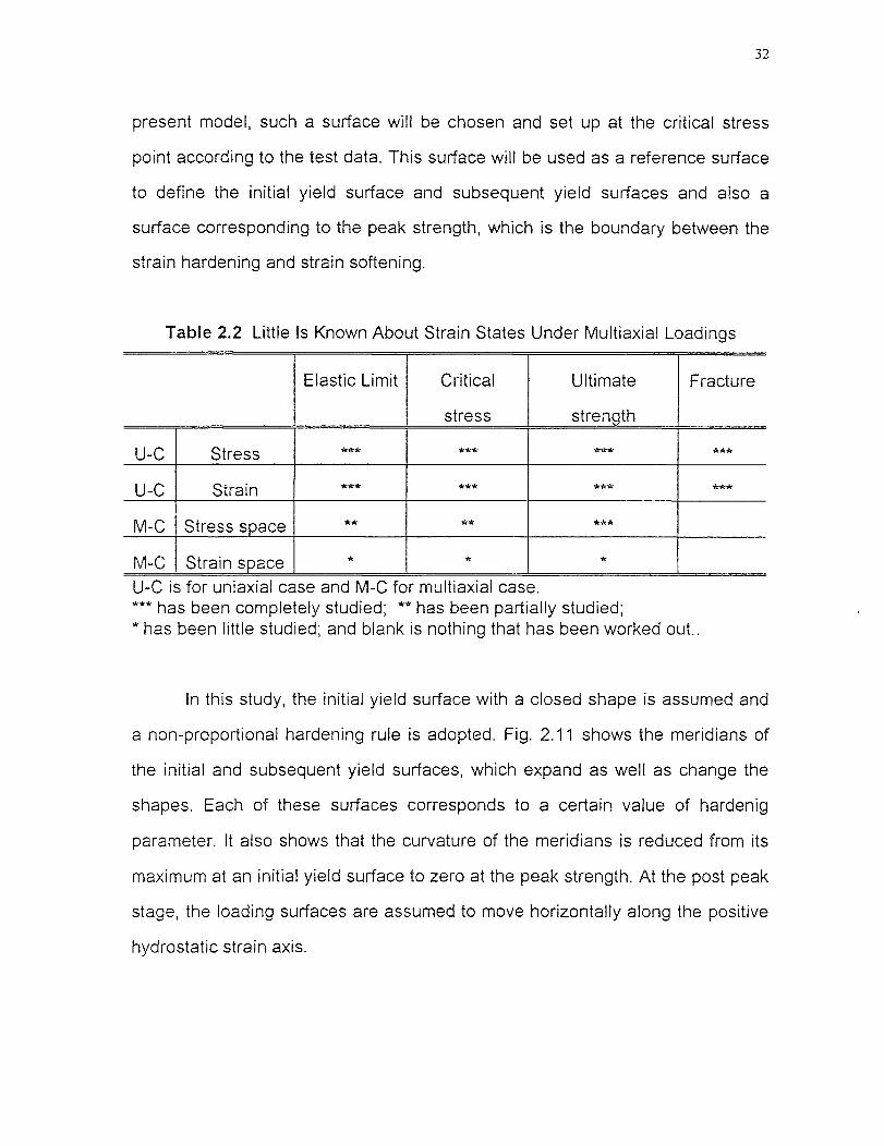
32

present model, such a surface will be chosen and set up at the critical stress

point according to the test data. This surface will be used as a reference surface

to define the initial yield surface and subsequent yield surfaces and also a

surface corresponding to the peak strength, which is the boundary between the

strain hardening and strain softening.

Table 2.2 Little Is Known About Strain States Under Multiaxial Loadings

Elastic Limit Critical

stress

Ultimate

strength

Fracture

U -C Stress *** *** *** ***

U -C Strain *** *** *** ***

M-C Stress space ** ** ***

M-C Strain space *U-C is for uniaxial case and M-C for multiaxial case.*** has been completely studied; ** has been partially studied;* has been little studied; and blank is nothing that has been worked out..

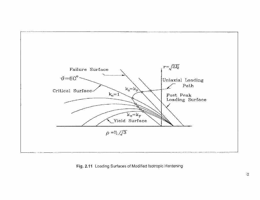
In this study, the initial yield surface with a closed shape is assumed and

a non-proportional hardening rule is adopted. Fig. 2.11 shows the meridians of

the initial and subsequent yield surfaces, which expand as well as change the

shapes. Each of these surfaces corresponds to a certain value of hardenig

parameter. It also shows that the curvature of the meridians is reduced from its

maximum at an initial yield surface to zero at the peak strength. At the post peak

stage, the loading surfaces are assumed to move horizontally along the positive

hydrostatic strain axis.

33

2.4.4 Hardening and Softening Control

The loading surfaces intersect the uniaxial compressive loading path. Then each

hardening parameter can be mapped to a certain value of effective strain and it

corresponds to a plastic modulus given by the experiment uniaxial compressive

plastic stress-strain curve (Fig. 2.12). However, it has been found out that the

plastic modulus defined by this approach can not predict the plastic stress

components adequately. Hence, a modification factor, as a function of the

volumetric stress and lode angle has been introduced to account for the

hydrostatic pressure sensitivity behavior. Then, the plastic modulus used is

equal to the original value multiplied by this factor.

In strain space, strain softening and strain hardening essentially have no

much difference. Softening is only a continued hardening after the stress state

reaches the ultimate value. In this model, the elastoplastic coupling or the

stiffness degradation is considered in the softening stage in a way analogous to

that of Han et al (1986).

2.4.5 Non-Associated Flow Rule

A non-associated flow rule is used to account for the large volume expansion of

the material. Here, a Drucker-Prager type of plastic potential with the dilatancy

factor taken as a function of hardening parameter has been assumed.

34

Fig. 2.9 Yield Surface with Open End

Fig. 2.10 Yield Surface with Closed End

ftY = 6 0°

Critical Surface k

/-.-----------------Yield Surface

1%141411111111

k o ky

ko=k

Failure Surface

Post PeakLoading Surface

Uniaxial LoadingPath

p =I /[

Fig. 2.11 Loading Surfaces of Modified Isotropic Hardening

36

Fig. 2.12 Plastic Stress-Strain Relationship

CHAPTER 3

STRAIN-SPACE CRITICAL SURFACE

3.1 Introduction

In plasticity theory, the yield surface is "a basic input of the material. For

concrete, yield criterion is a matter of definition and is usually a fictitious

quantity. It is used only for the convenience of mathematical modeling. The

general method in stress-space plasticity is using the failure surface as a

reference surface and defining the yield surface according to the failure surface.

The precondition for using this approach is that the reference surface is

available. If the yield surface in strain space is constructed in a similar way, a

strain-space reference surface is a must. Unfortunately, very little quantitative

information about strain state is known. Now the problem becomes where and

how to set up the strain-space reference surface. To best describe the material,

the reference strain state should be the one with an important physical meaning.

Also it must be relatively easy to be constructed, and convenient to set up other

surfaces.

3.2 Strain-Space Critical Surface

3.2.1 General

At the strain state during failure, the physical meaning is clear. It is naturally

considered as a possible reference surface. Analysis was made of available test

data of the strain state at the ultimate strength. But the result were very

scattered. The basic reason is that when the load approaches the peak value,

the stress state changes very little, while the strain state increases sharply, Thus

the stress-strain curve becomes flat and close to the horizontal line. This makes

37

38

it very difficult to determine the right strain state at peak strength. Further, the

brittle failure of concrete makes the obtained data not reliable (Gerstle (1980)).

In view of the loading system, the strain state is too sensitive to the test

environment. In short, an accurate strain measurement in the multiaxial loading

system is very hard to obtain when approaching the ultimate strength state.

Although with special attention, a good result may be obtained like that of

Kotsovos et al (1979), in practical use, the strain state at failure of a specific

concrete still suffers from the instability of strain state when trying to obtain the

basic input data. Because of this, the failure state in strain space is not chosen

as a reference surface. This was unexpected before performing the data

analysis on strain states of concrete.

Another important strain state is called the critical stress (Richard (1929)),

which corresponds to the minimum volumetric strain. The experimental data at

the critical stress are much more reliable. According to Shah et al (1968), when

the stress is beyond the critical stress, there is a sharp increase in the length of

continuous cross-linked microcracks. And this will cause concrete dilatation.

They pointed out that macroscopically, the critical stress is related to strengths

of concrete under short-term , repetitive and long-time loading, respectively. This

critical stress also affects the fracture toughness in a microscopic sense. It

indicates the beginning of significant slow crack growth. The states at the critical

stress was called 'onset of unstable fracture propagation' (OUFP) in the work of

Kotsovos and Newman (1977). And Newman and Newman (1972) used it for an

upper bound failure criterion.

Since the critical stress is such an important material parameter,

discussions of the corresponding strain states in a multiaxial case, which can be

called the critical strain state, is of significance. The corresponding surface in a

39

strain space herein is called "the critical surface", which is selected as a

reference surface for the strain-space yield surface.

At present, the strain state at the critical stress is not fully understood.

The test data are very limited and restricted mainly on the two situation: (1)

= 6 2 > 53 , and (2) 6, > e., = 53 . A quantitative expression of the critical surface

can only be achieved through appropriate assumption based on the existing test

data.

f ( 62) 63 ) = 0

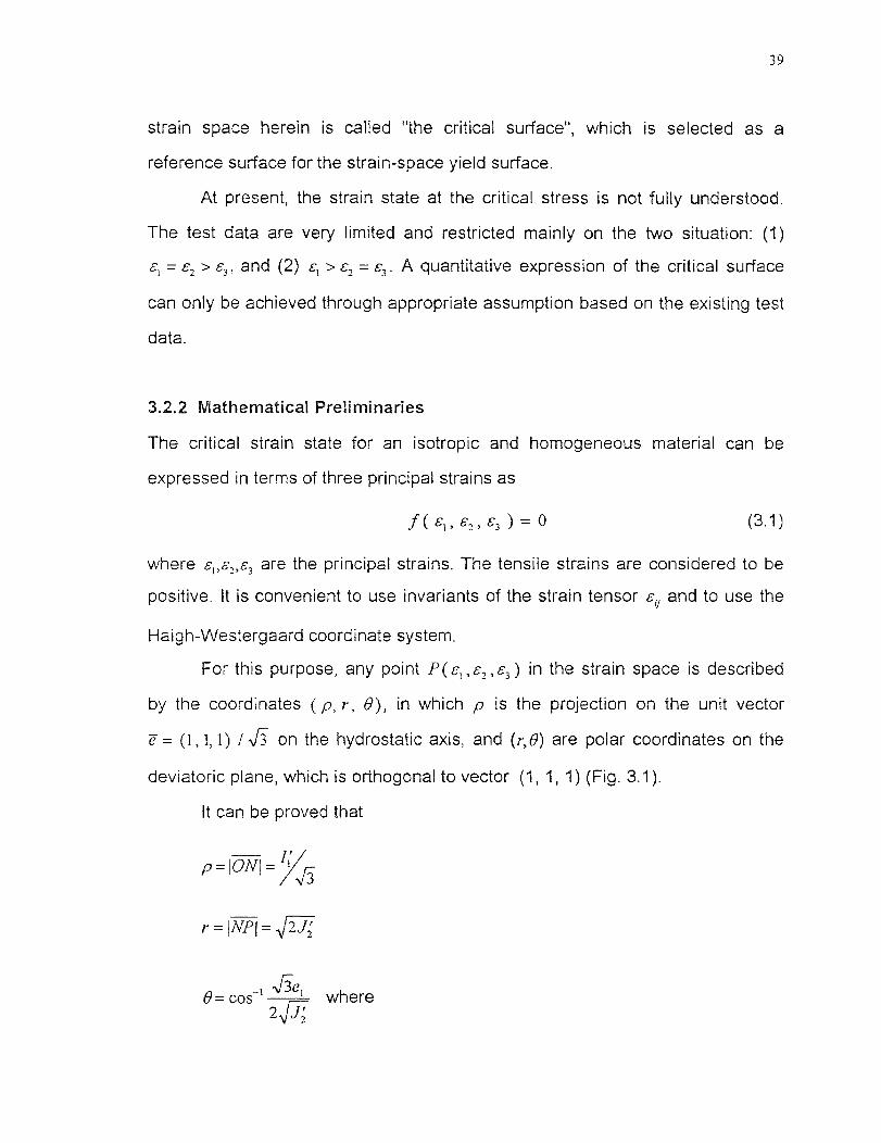
3.2.2 Mathematical Preliminaries

The critical strain state for an isotropic and homogeneous material can be

expressed in terms of three principal strains as

(3.1)

where 6- 1 ,6.2 ,6 3 are the principal strains. The tensile strains are considered to be

positive. It is convenient to use invariants of the strain tensor e u and to use the

Haigh-Westergaard coordinate system.

For this purpose, any point P(6 1 ,82 ,63 ) in the strain space is described

by the coordinates (p, r, 0), in which p is the projection on the unit vector

e= (1,1,1) / IA on the hydrostatic axis, and (r,9) are polar coordinates on the

deviatoric plane, which is orthogonal to vector (1, 1, 1) (Fig. 3.1).

It can be proved that

,p=10N1= 17—-,13

r =INPI= .i2J;

Nrie9= cos , where

40

e l = — for ei > 52 > e,

iri'= El ± E2 ± 63

= 6 yet -

62 )2 ±(62 83 )2÷(63 632]

in which, p represents the hydrostatic component, r is a deviatoric component,

and 9 is called Lode angle. 1 1 is the first strain invariant and J 21 is the second

deviatoric strain invariant.

Therefore, Eq.(3.1) can be stated more conveniently as

f (p, r, 0) = 0 (3.2)

Assume that the concrete is an isotropic material, the labels 1, 2, 3

attached to the coordinate axes are arbitrary. Thus, the cross-sectional shape of

the surface must have a threefold symmetry shown in Fig. 3.1(a). Therefore, it is

necessary to explore only the sector from 0= 0° to 0= 60° , the other sectors

can become known by symmetry.

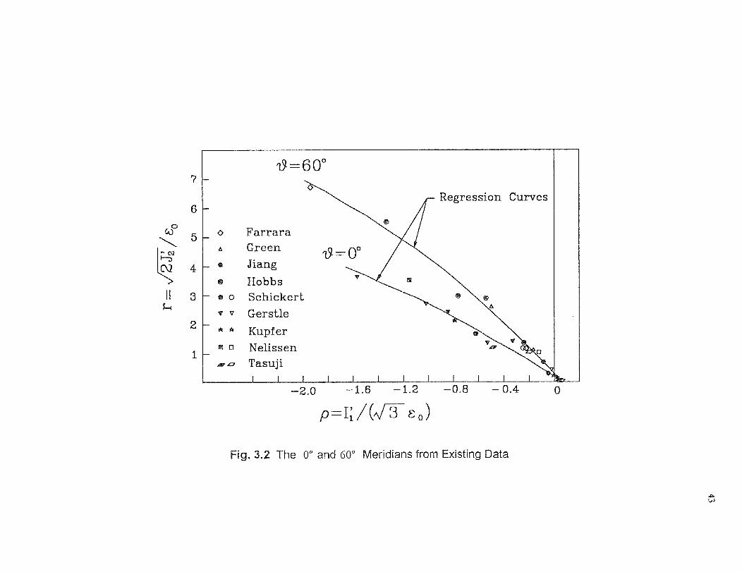
3.2.3 General Properties of Critical Surface

In an experimental determination of critical surface, as it appears in the Haigh-

Westergaard coordinate system of Fig. 3.1, 0= 60° meridian (e l = 62 > £3 ) and

0° meridian (e, > e., = 63 ) are essential to construct such a surface. On the

basis of test data by Kupfer et al (1969), Hobbs (1974), Green and Swanson

(1973), Jiang et al (1991), Gerstle (1980), Tasuji et al (1978), Schickert and

Winkler (1977), Ferrara et al (1976), and by Kotsovos and Newman (1979), the

0 and 60-degree meridians are found by the regression curves as illustrated in

Figs. 3.2 and 3.3. In Fig. 3.2, since the data are from different tests, all the

reading are nondimensionalized by the uniaxial strain value at the critical

41

Fig. 3.1 Haigh-Westergaard Strain Space

LP

stress. Both figures show that the meridians are curved, smooth, convex and r

value increases with increasing hydrostatic strains p, and that ro lr., where the

indices 0 and 60 represent 0 and 60 degree meridians respectively, lies between

0.5 and unity.

From these features, one may conclude that the critical surface in strain

space is a cone shape with smooth curved meridians and convex sections

between circular and triangular shapes on the deviatoric strain plane.

3.2.4 Formulation of Critical Surface in Strain-Space Domain

With the analogy of the strain-space critical surface to that of the stress-space

failure surface of concrete, similar mathematical formulations from the available

stress-space failure surface is found useful. A possible critical surface function

in Hsieh-Ting-Chen form is given below (Hsieh, Ting, and Chen 1982).

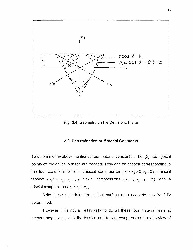
Fig. 3.4 shows a possible critical surface cross-section on the deviatoric

plane. For a constant value k, rcos6=k represents an equilateral triangle, and

r=k is a circle on the deviatoric plane with VA 0. Hence, for given two positive

constants a, /3 with a+,6= 1, a combined equation r (acos0+ 13) = k yields a

smooth function between ltSI 60° on the deviatoric plane and it is bounded by

the two extremes of equilateral triangular and circular shapes (a= 0,p , 0).

Recall the convex meridians in Figs. 3.2 and 3.3. This indicates that for a

constant value of 0 and r, there is a nonlinear parabola-like function of p. Hence,

p and r 2 terms are added and the resulting form is given by,

f(p,r, 0)= ar 2 + (acos( 9 - - P)r + c p — =0 (3.3)

where the parameter can be nondimensionalized by using the uniaxial

compressive strain value at critical stress. The four parameters a, a, 1 1 and c

are material constants, which need to be evaluated.

Regression Curves

rt5t =0°

1 I 1 1 1 I 1 1 I

19 60°

o Farrara• Green

_ 0 Jiang

• Hobbs• 0 Schickert✓ v Gerstle

A Kupfer• Nelissen

L:7 Tasuji

—2.0 —1.6 —1.2 —0.8

0

P = IAN/YE0

Fig. 3.2 The 0° and 60° Meridians from Existing Data

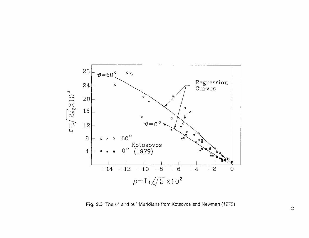
Fig. 3.3 The 0° and 60° Meridians from Kotsovos and Newman (1979)

28

24CDo

20X

- C\1 16C\2

12

8

4

p=f1/ 3 x10 3

—14 8 —612 —10 —4 2 0

RegressionCurves

0

o v ❑ 60 °Kotosovos

• 0 ° (1979)

rcos 19-=kr(a cos19 + # )=kr=k

45

Fig. 3.4 Geometry on the Deviatoric Plane

3.3 Determination of Material Constants

To determine the above mentioned four material constants in Eq. (3), four typical

points on the critical surface are needed. They can be chosen corresponding to

the four conditions of test: uniaxial compression ( = e, > 0, 6. 3 < 0 ), uniaxial

tension ( > 0, 62 = E3 < 0 ) , biaxial compressions ( > 0, 6, =E3 0 ), and a

triaxial compression ( 8, 83

With these test data, the critical surface of a concrete can be fully

determined.

However, it is not an easy task to do all these four material tests at

present stage, especially the tension and triaxial compression tests. In view of

46

lacking of basic test data, the following method is suggested to approximately

calculate the results of tensile tests from the uniaxial compression result. This

approximate method is based on assumptions: 1) When under tension, the strain

states deviate little from those computed with Hooke's law (Kupfer et al (1969),

Wastiels (1979)). 2) Tensile strength in one direction is not affected by the

tensile actions on the other direction (Ahmad (1981), Tasuji et al (1978)). 3)

Under tensile action, the critical strain state can be chosen to be about 95

percent of the strength. 4) The uniaxial tensile strength is approximately equal to

f .0.295 ( Jr' ,ft and fc' are in N/mm2 ) (Wastiels (1979)).

Further, the poisson's ratio and the modulus of elasticity in tension are

assumed to be the same values as those in tension, respectively. With above

assumptions, the strain state at the critical stress in tension can be computed

approximately by using the Hooke's law.

The confined uniaxial compressive test can give a point under triaxial

compression. In the case of no triaxial compressive data,

) = ( 2 , 63 ) on the 60-degree meridian can be used,

which seems to give the best fit to the test results by Kupfer et al (1969). s o here

is the strain at critical stress on the uniaxial compressive stress-strain curve.

3.4 Verification and Discussion of Formulated Surface

From the limited available test data, the parabola-like meridians are obtained.

According to the 0 and 60 degree meridians together with the reasonable

deduction, the general shape of critical surface is given in Eq. (3.3). To verify

that Eq. (3.3) is valid for the strain combination not on the 0 or 60 degree

meridians, comparison is needed between the test data and prediction of the

47

formula proposed. The most efficient way is to check on the deviatoric plane.

Test results of Kupfer et al (1969), Schickert and Winkler (1977),and Nelissen

(1972) are adopted.

3.4.1 Comparison with Test Data of Kupfer et al (1969)

The material constants used are modulus of elasticity E=31700 MPa; Poisson's

ratio /I= 0.22 ; uniaxial compressive strength 41 = 32.2 MPa and the strain at the

critical stress for uniaxial compression e= 0.00153 mfrn.

Table 3.1 gives the four basic input points to determine the critical

surface. The four constants are determined as shown in Table 3.2. Fig. 3.5

shows the comparison between the test points and the predicted results.

Table 3.1 Basic Input for Kupfer et al 's Critical Surface

r (0.001) p ( 0.001) 9 (degrees )

Uniaxial Compression 1.5690 -0.4307 60

Biaxial Compression 3.3117 -1.1605 0

Uniaxial Tension 0.1050 0.043 0

Triaxial Compression 9.6390 -3.060 60

Table 3.2 Critical Surface Constants of Kupfer et al 's

a a fl c

5015.0 2434.0 2442.0 11350.0

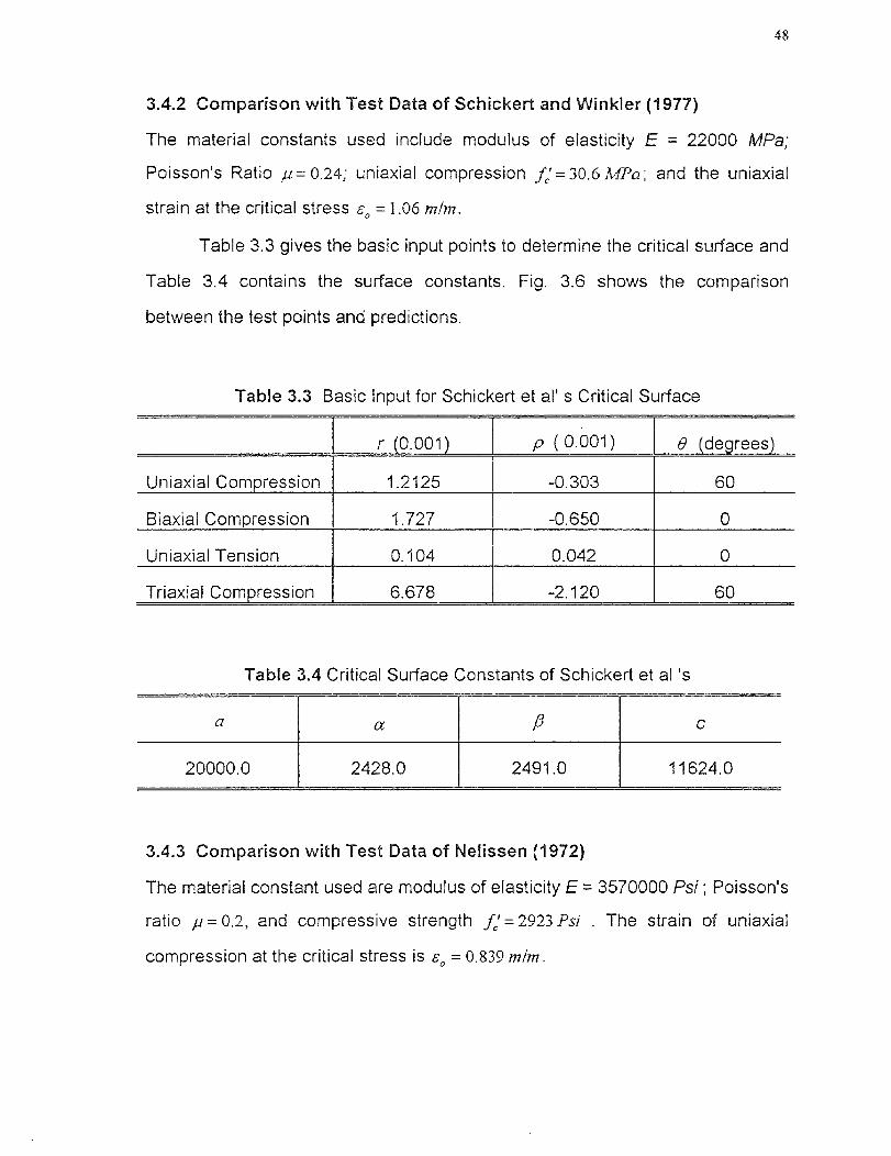
48

3.4.2 Comparison with Test Data of Schickert and Winkler (1977)

The material constants used include modulus of elasticity E = 22000 MPa;

Poisson's Ratio p= 0.24; uniaxial compression f;=30.6MPa; and the uniaxial

strain at the critical stress so =1.06 m/m.

Table 3.3 gives the basic input points to determine the critical surface and

Table 3.4 contains the surface constants. Fig. 3.6 shows the comparison

between the test points and predictions.

Table 3.3 Basic Input for Schickert et al' s Critical Surface

r 0.001 p (0.001) 0 de rees

Uniaxial Compression 1.2125 -0.303 60

Biaxial Compression 1.727 -0.650 0

Uniaxial Tension 0.104 0.042 0

Triaxial Compression 6.678 -2.120 60

Table 3.4 Critical Surface Constants of Schickert et al 's

a a 13 c

20000.0 2428.0 2491.0 11624.0

3.4.3 Comparison with Test Data of Nelissen (1972)

The material constant used are modulus of elasticity E = 3570000 Psi ; Poisson's

ratio /./. 0.2, and compressive strength f:= 2923 Psi . The strain of uniaxial

compression at the critical stress is ea = 0.839 mini.

49

Table 3.5 contains the basic input points for the critical surface, and Table

3.6 gives the constants of the surface. Fig. 3.7 shows the comparison between

Nelissen's test points and the formula predictions.

Table 3.5 Basic Input for Nelissen' s Critical Surface

r (0.001) p ( 0.001) 9{degrees )

Uniaxial Compression 0.887 -0.199 60

Biaxial Compression 3.055 -0.968 0

Uniaxial Tension 0.1058 0.0374 0

Triaxial Compression 5.034 -1.678 60

Table 3.6 Critical Surface Constants of Nelissen 's

a a 16 c

35000.0 2641.0 2323.0 11471.0

3.4.4 Strain State of High Hydrostatic Compression

The experimental points and the prediction by Eq. (3.3) on the deviatoric plane

are shown in Figs. 3.5-3.7. It can be seen that the prediction is satisfactory.

In stress-space analysis, the concrete undergoes no failure in a

hydrostatic compressive state a, =a-2 = a3 . This feature also holds in the strain-

space analysis. However, the stress surface can extend with no limit along the

hydrostatic axis, but the strain-space critical surface should have an upper limit

on the hydrostatic axis because the volume of concrete can not decrease without

limit under the hydrostatic loading. Thus , the critical surface is within a range on

the hydrostatic axis. The upper limit is on the top of the cone, and the lower limit

50

is corresponding to the minimum volumetric strain under hydrostatic action.

(From triaxial hydrostatic compression test of Schickert and Danssmann (1984),

under 150 MPa, the volumetric strain reached -0.0125 m/m ). The possible

minimum value, the shape of limit surface and the open end of critical surface,

are the problems to be studied all together with the related experimental data. In

spite of these uncertainties, the critical surface is still found to be useful for non-

high-hydrostatic compressive situation.

Fig. 3.5 Test Points by Kupfer (1969) and Formula Prediction

p= — o. 78 (mm/m)

/3=-0.65

p= —0 .40

• Tested by Schichert (1977)

51

Fig. 3.6 Test Points by Schickert (1977) and Formula Prediction

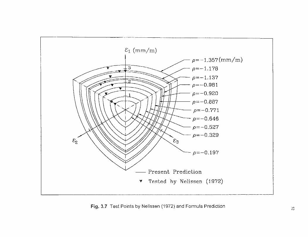
CHAPTER 4

PROPOSED CONSTITUTIVE EQUATION

4.1 Introduction

Plasticity method is a phenomenological method. Its aim is to reproduce

mathematically the macroscopic stress-strain relations for different loading

conditions, neglecting the microscopic mechanism of the behavior. To set up a

plasticity model, three components are essential. They are (1) an initial yield

surface that defines the level in stress space or in strain space at which plastic

responses start ; (2) a hardening rule that defines the change of the loading

surface as well as the change of the hardening properties of the material during

the course of plastic flow; and (3) a flow rule that is related to a plastic potential

function and gives an incremental plastic stress-strain relation. The present

strain-space plasticity model is also basically following the similar principles.

Since the classical theory of plasticity is developed in the stress space, many

assumptions and modifications are needed to apply in applying the plasticity

theory to the strain-space version for concrete.

4.2 Yield Criterion

4.2.1 General Description

Yield criterion defines the elastic limit in a multiaxial stress state or its strain

counterpart. For metals, the yield condition is used as a failure criterion, and is

determined by the tests. The yield state for concrete is a fictitious quantity, and

is used only in the mathematical constitutive law. In stress-space plasticity

methods, the failure surface of concrete is considered as reference surface. For

53

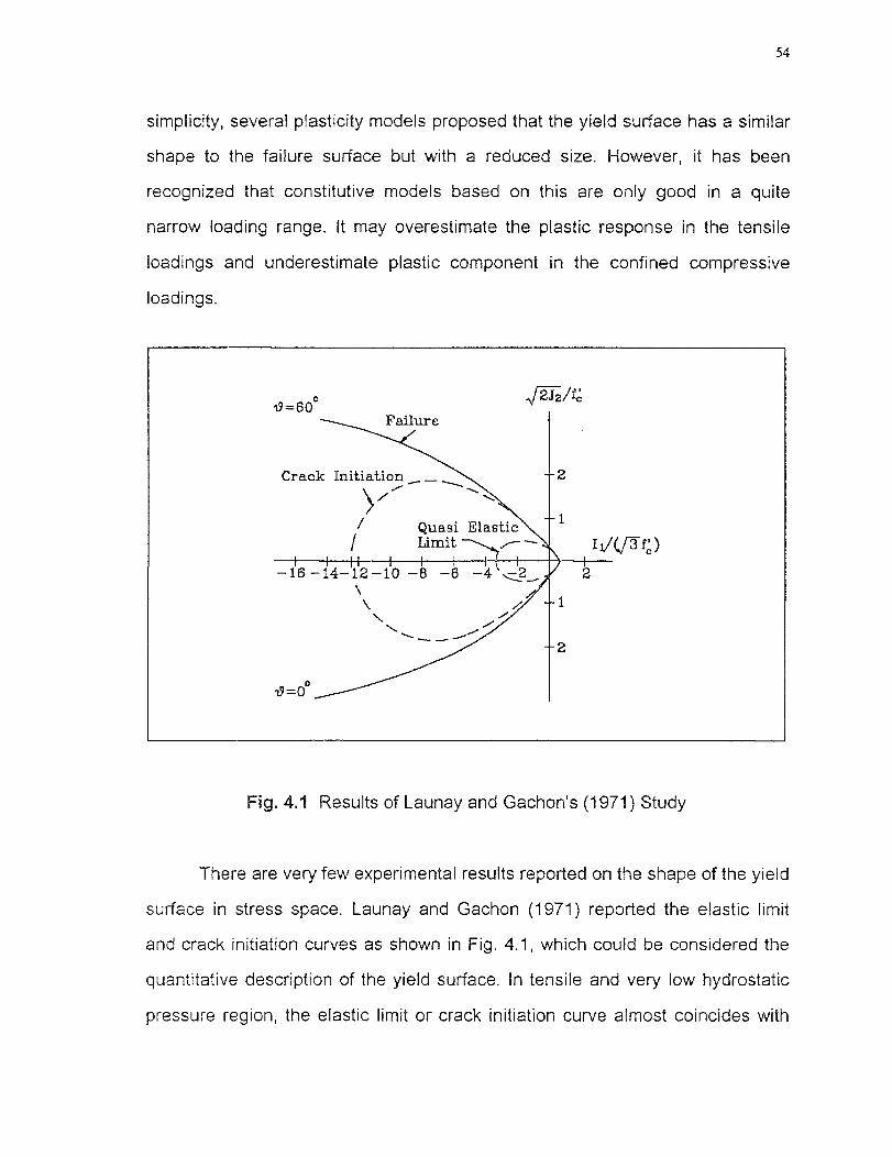
54

simplicity, several plasticity models proposed that the yield surface has a similar

shape to the failure surface but with a reduced size. However, it has been

recognized that constitutive models based on this are only good in a quite

narrow loading range. It may overestimate the plastic response in the tensile

loadings and underestimate plastic component in the confined compressive

loadings.

Fig. 4.1 Results of Launay and Gachon's (1971) Study

There are very few experimental results reported on the shape of the yield

surface in stress space. Launay and Gachon (1971) reported the elastic limit

and crack initiation curves as shown in Fig. 4.1, which could be considered the

quantitative description of the yield surface. In tensile and very low hydrostatic

pressure region, the elastic limit or crack initiation curve almost coincides with

Critical Surface

Yield Surface

55

the failure curve, and the hardening-plastic zone has vanished. In a compressive

region with hydrostatic confining pressure, the hardening zone can be quite

large. It has been widely accepted that in stress space concrete has a closed

initial yield surface.

In strain space, Kotsovos (1978) gave the similar closed-ended elastic

limit shape, as the one in stress space (See Fig. 2.3).

Fig. 4.2 Strain-Space Yield and Critical Surfaces

Based on this observation and the stress-space counterpart, the

proposed shape of the initial yield surface in strain-space is shown in Fig. 4.2.

Here the critical surface is the reference. This initial yield surface coincides with

the critical surface in the small compressive hydrostatic strain and tensile

hydrostatic strain regions, and has a closed end along the compressive

hydrostatic strain axis.

56

The subsequent yield surface, also called the loading surface defines the

boundary of the current elastic region for an elastoplastically deformed material.

If a state point (either in stress space or in strain space ) lies within the region,

no additional plastic response takes places. On the other hand, if the state point

is on the boundary of the elastic region and tends to move out of the current

loading surface, additional plastic response occurs. In other words, the current

loading surface will change its current configuration when plastic response takes

place. Thus, the loading surface may be generally expressed as a function of the

current state of stress (or strain) and some hidden variables. In strain space, one

may have the loading surface

ko)= 0 (4.1)

where the hidden variables are the plastic strain sl; and a hardening parameter

k0 .

4.2.2 Formulation of Initial Yield Surface and Subsequent Yield Surfaces

The critical surface function given by Eq. (3.3) can be rewritten as

f (p,r,0)=r — = 0 , 1015_ 60° (4.2)

where

= rc ( jo, 0) = [— (a cos0+ ) + (acos 0+13) 2 — 4a (c,o— 1)] ( 2a )

With the critical surface in Eq. (4.2) as the reference, the yield surface

and subsequent yield surfaces are expressed in the form of

F (p, r , 0, ko )= r — k rc = 0 , 1015_ 60° (4.3)

where k = k(p, Ice ) is a shape factor which is a function of hydrostatic strain p,

and a size parameter ko . This shape factor modifies the critical surface so as to

give a proper shape for the initial yield surface and subsequent yield surfaces.

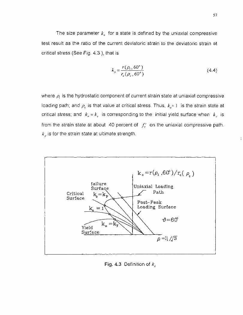
ka r=r(Pi, ,60 )/r.( Pe )

failureSurfa e

Critical kb =kpSurface

YieldSurface

Uniaxial LoadingPath

Post—PeakLoading Surface

57

The size parameter ko for a state is defined by the uniaxial compressive

test result as the ratio of the current deviatoric strain to the deviatoric strain at

critical stress (See Fig. 4.3 ), that is

k = r

(PI ' 60°)

° rc.(p, , 60°)(4.4)

where A is the hydrostatic component of current strain state at uniaxial compressive

loading path; and pc is that value at critical stress. Thus, ko= 1 is the strain state at

critical stress; and k, = ky is corresponding to the initial yield surface when ky is

from the strain state at about 40 percent of f' on the uniaxial compressive path.

kp is for the strain state at ultimate strength.

Fig. 4.3 Definition of ko

58

The shape factor k =k(p,k0 ) is assumed as a parabola before reaching

the critical surface. From on the critical surface till the failure surface,

k = k ( p, = k, , which is a horizontal line. The parabola requires three points to

determine: (p„1) , ,0 ) and (p l , k, ) , where pc represents the dividing point

for tensile and compressive regions; and is around 0; p -gives a(1-ka )

closed end of the loading surfaces. A is a constant, which can be calibrated

according to the Launay and Gachon's result (1971). When ko approaches 1, 7),

goes to infinity and the loading surface reaches the critical surface. p = p i (ko )

is the relation between the hydrostatic strain of uniaxial case and ko . For a strain

state, this relation actually gives the hydrostatic component of the corresponding

state point on the uniaxial compressive path, which can be obtained from the

uniaxial compression test data. k i is the ratio between the deviatoric strain of

uniaxial compression at ko , to the deviatoric value of 60 degree meridian on the

critical surface at pi . Fig. 4.4 shows the relation between ko , k, , and p i . From it ,

one can easy find

AC rc(p„ 60° )AB _ ko rp ( pc , 60°)

(4.5)

The shape factor for ky , where k y is corresponding to ko , may be

in the following form

1 pi)k(p,ko )= k (pi > p>T5)

(4.6)

0 ( 5 ?.p)

where

[(o — P)—k " '— r5) 1 ( 02 -152 )+[(P2,- To2 -Pi - 7,2 )1(P-P) kp= 152 )(P — To) —(14 — TO' )( 15)

Fig. 4.5 is a graphic description of the shape factor.

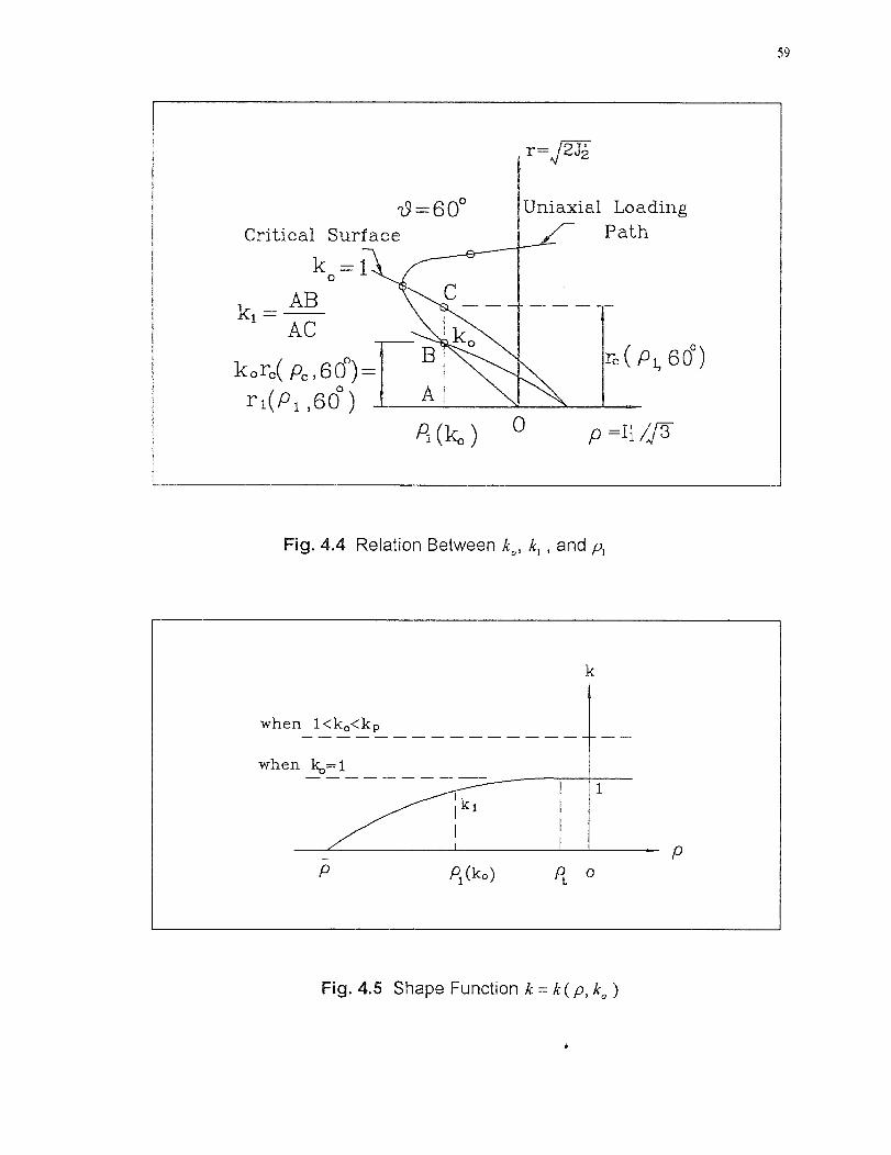
Uniaxial LoadingPath

59

Fig. 4.4 Relation Between ko , k 1 , and pl

Fig. 4.5 Shape Function k=k(p,ko )

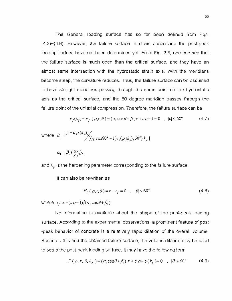
60

The General loading surface has so far been defined from Eqs.

(4.3)-(4.6). However, the failure surface in strain space and the post-peak

loading surface have not been determined yet. From Fig. 2.3, one can see that

the failure surface is much open than the critical surface, and they have an

almost same intersection with the hydrostatic strain axis. With the meridians

become steep, the curvature reduces. Thus, the failure surface can be assumed

to have straight meridians passing through the same point on the hydrostatic

axis as the critical surface, and the 60 degree meridian passes through the

failure point of the uniaxial compression. Therefore, the failure surface can be

Ff(e9 )= Ff ( p,r, 0)= (a l cos 0+ 161 )r + c p - I = 0 (6<_60° (4.7)

where /31 = [1 — c p,(k p )]

R cos60° +1) rc ( Jr),(k 0 ),60°) k p ]

ar = /31 (

and k p is the hardening parameter corresponding to the failure surface.

It can also be rewritten as

Ff (p,r, 0)=r —rf =0 161 60°

(4.8)

where rf = —(cp— 1)/(a 1 cos e+ ,g,) .

No information is available about the shape of the post-peak loading

surface. According to the experimental observations, a prominent feature of post

-peak behavior of concrete is a relatively rapid dilation of the overall volume.

Based on this and the obtained failure surface, the volume dilation may be used

to setup the post-peak loading surface. It may have the following form

F ( p, r , 0,k,, )= (a, cos0 ± A) r + c p— y(ko )= 0 , I61 <_ 60° (4.9)

Failure Surface niaxial LoadingPath

(ko—kp )• r( Pe , 8CP)

Critical Surface

16= 6 0°

Post PeakLoading Surface

p=Ii/Ja Pp

r=

61

where y(k0 )= cpo - 1 for p, and po is a function of ko . From Fig. 4.6 , po is

determined when pi (ko ) is known.

The rewritten version is

F (p, r , 9,ko )= r — ro = 0 , 16i 60° (4.10)

where ro = [ y(ko)—cpjl(a 1 cos0- A).

Fig. 4.6 Relationship Between Failure Surface and Post-Peak Loading Surface

62

4.3 Hardening Rules

4.3.1 General

The post yield response, called the hardening rule, is described by specifying

the rule for the evolution of the subsequent yield surfaces. Several hardening

rules have been proposed in the past for use in plastic analysis. The most widely

used rules are those of isotropic hardening, kinematic hardening, and a

combination of both, which is called mixed hardening. In this study, a modified

isotropic hardening rule and a kinematic hardening rule are used.

4.3.2 Modified Isotropic Hardening Rule

The isotropic hardening rule assumes that the initial yield surface expands

uniformly without distortion and translation as the plastic flow occurs. In the

modified isotropic hardening rule, the initial yield surface expands in the way as

seen in Fig.2.11, rather than uniformly.

In the previous discussion, one can see that in the loading function Eq.

(4.3) the size parameter ko plays an important role in defining the loading

surface, With a given ko , the corresponding loading surface can also be

determined. This size parameter is called the hardening parameter in theory of

plasticity. With k o changes from ky to 1 and further to kp , the loading surface

goes from the initial yield surface, through the critical surface and to the ultimate

surface. In Fig. 2.11, with the strain hardening continues, the loading surface

change from the initial close-ended shape to the open-ended surface. Since the

shape factor is independent of the Lode angle 6' , the loading surface on the

deviatoric plane only changes its size, but not the shape.

One argument about this modified isotropic hardening procedure is what

action mechanism causes this yield phenomenon if the loading path is along the

63

hydrostatic strain axis. The possible cause is the damage in the crushed pores

or small holes. Although detailed and satisfied explanation is not available, the

experimental research of Schickert and Danssmann (1984) did show that the

progressive damage occurred under the increasing hydrostatic pressure action.

In their test, they first applied the hydrostatic pressure with different values on

the same batch of concrete cubic specimens. After taking off the pressure, they

measured the change in ultrasonic pulse velocity and the uniaxial compressive

strength. The results were quite consistent that the hydrostatic pressure cause

the damage to the material structure.

4.3.3 Effective Strain and Plastic Effective Stress

To use the plasticity theory, one must relate the hardening parameter in the

loading function to an experimental uniaxial compressive stress-strain curve. To

this end, effective strain and effective stress must be defined, so that they can

be plotted against each other and used to correlate the test results obtained by

different loading programs. Further, the effective stress-strain curve could be

calibrated against the uniaxial compressive stress-strain curve.

For a uniaxial compression, the loading function, Eq. (4.3) is expressed

F= ri, — k(p, ko ) rc ( p i , 60°) = 0 (4.11)

where

and /9, = p i( ).

as

Let e = — E3 and substitute it into Eq. (4.11). Then, the effective strain is

defined as

64

e k(p i ,ko )r(p i , 6O 0 ) - 17 1/-1/3 (4.12)=

Actually in this model, the effective strain is the uniaxial compressive

strain for the given strain state.

The corresponding plastic effective stress CY p is hereby defined in terms of

the plastic energy density

aPP = a d< = s dap (4.13)

where a is the effective stress, e t,P and < are the plastic and elastic components

of effective strain s, respectively. The relationship between the elastic and

plastic components and the plastic work increment is shown in Fig. 4.7 and Fig.

4.8, respectively

On the other hand,

dw = 8;. dari = d2 & if(4.14)

where, e. is the elastic component of strain tensor s ,, ul; is the plastic

component of stress tensor au ., a non-associated flow rule is used here. G is the

plastic potential function and d2 is a positive scalar. Hence, according to the

energy conservation law, by setting Eqs. (4.13) and (4.14) equal, the effective

plastic stress may be expressed as

do- p = d2 (4.15)

where

e eG I s:de

de

CPI

65

Fig. 4.7 Relationship Between Elastic and Plastic Components

Fig. 4.8 Plastic Work Increment

66

4.3.4 Effective Strain and Plastic Effective Stress Relation

The effective strain-plastic effective stress relation, characterizing the hardening

processes of material, is now calibrated on the uniaxial compression test, which

has the form

orp = o-p(e,) (4.16)

The graphic expression and its relation with the general uniaxial stress-strain

relationship were shown in Fig. 2.12.

Differentiation with Eq.(4.16) gives the following incremental relation

do - p = 11;(6e ) dee (4.17)

where I- (cc ) is a plastic modulus associated with rate of expansion of the yield

or loading surfaces; and is the slope of the uniaxial plastic stress-strain curve at

the current value of c e .

4.3.5 Relationship Between Hardening Parameter And Plastic Modulus

The hardening parameter k is a function of plastic work and is related to plastic

modulus .11; which is derived from a uniaxial compressive curve. For a uniaxial

compression, the loading function becomes

Fu (p,,ru , 60°, k o )= ji (p,113+ ee ) — k(pl ,ko ) rc(pl , 60°) = 0 (4.18)

In this equation, the effective strain se .and hardening parameter ko are

variables. Differentiating the equation gives

dFu = c2F

u dk° +

OFu de

e

=0alko Os,

(4.19)

dk o = yr dee (4.20)

where

67

tit=oFo of.02e gko

OFu 1 op; ek gp, dk )7. k Op, Oko J2 Oka 5p, dko Ok 0 C OA a°

In such a manner, each loading surface or parameter ko is related to an

effective strain ee , further to a plastic modulus Hp, also to the plastic work,

implicitly.

4.3.6 Influence of Multiaxial Loading on Plastic Level

The plastic modulus Hp, taken from the experimental uniaxial compression test,

is called the basic plastic modulus. It is fixed for a given loading surface, which

represents a certain level of working-hardening. When it is zero, the material is

in elastic stage. The larger it is, the stronger the plastic response is. Since it is

taken from the uniaxial compression test, it may not be right to be used to

describe the plastic degree for the multiaxial loading situation. Modification is

necessary.

Multiaxial loadings may influence the plastic level of material mainly in

two ways. The first is to change the confinement action. In the case of

compression with confining pressures, concrete becomes more ductile. The

other is to change the Lode angle. The former can be seen obviously in such

normalized stress-strain curves as Fig. 4.9. The latter means with the same

confinement action, the plastic procedure will be different if different loading

direction on the deviatoric plane is followed since the loading surfaces are not

circular.

0 1.0

10

Compressionwith LateraConfinement

Compressionwith LateralTension

UniaxialCompression

max

Perfect Plasticituation

LinearElasticSituation

68

in Fig. 4.9, the closer the curves to the perfect plastic lines OAB, the

higher the plastic level the material undergoes. In other words, if the curve is

closer to the 45 degree straight line, the less inelastic response will be. From

this point of view, when the curve discussed is above the uniaxial curve, the

plastic level is higher and the plastic modulus must be larger than the basic

plastic modulus H; . On the contrary, when the curve is below the uniaxial

curve, a reduced value should be adopted.

To take into account of confinement, ps = , the hydrostatic pressure

in stress space is used. Thus, the influence of multiaxial loadings on the plastic

level can be described by using a modification function of jos and 9 to H; . The

modified plastic modulus is the equivalent plastic modulus for general case,

which is then expressed as

Fig. 4.9 Normalized Stress-Strain Curves

69

Hp = M(p, 0) H; (4.21)

where the modification factor Al(ps, 9) is simply constructed in the form

M(P.,, 9) = MI(A) M2( 0 ).

By assuming that the influence of the multiaxial loadings to the plastic

response is the same as other different states, it becomes much easier to

determine this modification factor from the test data.

M(p,, 9) is considered with two different situations. One with the

confinement larger than that of the uniaxial compression, called case one; the

other with confinement less than that of the uniaxial compression, called case

two. Since H; is taken from the uniaxial compressive state, it is valid for the

situation in which the hydrostatic stress p, is about Thus, when p, is

smaller than which means larger confinement action than uniaxial

compression, modification is needed. In a concrete cylinder compression test

with confining pressure, as reported by Palanisway et al (1974) that there exists

a transition confining pressure and it is around the value of f; They concluded

that when the confining pressure was less than f.', the increasing plastic

response was observed with the increasing confining pressure (concrete exhibits

more ductile behavior). However, if the confining pressure was greater than f c.',

the plastic response became smaller with the increasing pressure and less

ductile failure behavior was found. Fig. 4.10 was the graph from their paper. Fig.

4.11 expresses the curves in the plastic stress-strain form. M1 ( p) is derived on

the basis of this test result.

According to Han (1985), for the situation with the same hydrostatic

pressure, the stress state at 60 degree meridian induces about two times as

much as that is induced by stress state at the 0 degree meridian . For the strain

state, in view of lacking the experimental information, the same effect as stress

state is used.

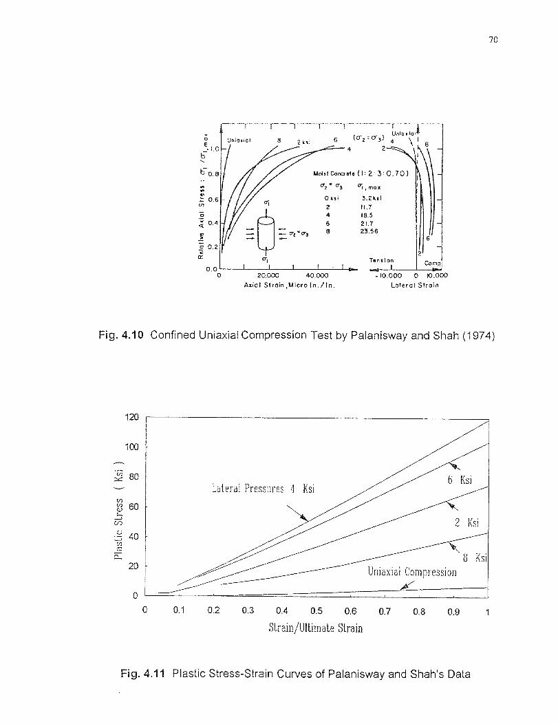
8

0.0

2 kI 6 (Crz ) 4 \

4

Un l o ia l

Meisl Corcyme ( I: 2: 3- 0.70 )

crx O cri , TO X

0 k3 I 3.2 kil

2 11.74 18.56 21.78 23.56

b

b 0 8

0.22

0 20.000 40.000

Axial Strain ,Micro In./In.

00 MP O.°10.000 0 10.000

Lateral Strain

cr, Tension

120

100

80

20

0

Lateral Pressures: 4

2 Ksi

8 KsiUniaxial Compression

Fig. 4.10 Confined Uniaxial Compression Test by Palanisway and Shah (1974)

70

0 0,1 0.2 0.3 0.4 0.5 0.6 0.7 0.8 0.9 1

Strain/Ultimate Strain

Fig. 4.11 Plastic Stress-Strain Curves of Patanisway and Shah's Data

71

Based on the above analysis, the modification function for case one

situation can be given

M(ps, 9)= { - 1.04 (4.5 -1--tkl ) 2 +17.5 ( 1.5 - cos0) (4.22)

where /1 = CY + + Cr3 is the first invariant of stress tensor uo .

Case two may occur when combined tension and compression exist

simultaneously. The contribution of Lode angle 0 to the modification function

can be ignored in this low hydrostatic pressure region. Thus, the case two is the

region between OA and OC in Fig. 4.12, where OA is the uniaxial compressive

loading path, OB is the uniaxial tensile loading path. For the stress state on OA,

M(ps, 0) =1, and on OC, AAA, 0)=0. The transition of the plastic level from

uniaxial compression to uniaxial tension is assumed here as a parabolic

function. Therefore, the modification factor is

Fig. 4.12 Tensile Influence on AAA, 0)

72

Al(p,,O)=( ft- 1,00, 1 ) 2 1 (1. 1,00, ) 2 (4.23)

where pa4 the hydrostatic stress for the uniaxial compression, which is

determined from the uniaxia stress-strain curve for a given k0

4.3.7 Kinematic Hardening Rule

In addition to the shape and size changes, the loading surface may also act like

a rigid body translating in the strain space. This is called kinematic hardening

(Fig. 4.13). This hardening rule provides a simple means of accounting for the

Bauchinger effect, which is a type of directional anisotropy. The key to a

subsequent yield surface based on a kinematic hardening rule is the

determination of the coordinates of the center, au , which can be changed with

the plastic response. Then, the loading surface becomes

k o ) = I - k(o,k0 )Fo = 0 (4.24)

in which ir , ;5 and F, are calculated by the same equations but with = - a.

In this model, the kinematic hardening is used between the critical surface and

the failure surface. The translation of the loading surface in strain space is given

according to Panos (1987) as

a.. = SU P1.1

(4.25)

which implies the local unloading with the initial elastic stiffness for a uniaxial

compression. When a state of strain is in the hardening stage, the total strain

increment is always larger than the plastic strain increment; thus with this

kinematic hardening rule, the loading surface will expand outward as well as

move in the space.

Subsequent LoadingSurfaceFailure

Surface

Initial YieldSurface

ElSubsequent Loading

SurfaceFailureSurface \

C3 C2

Initial YieldSurface

73

(a) Isotropic Hardening

(b) Mixed Hardening

Fig. 4.13 Hardening Rules

(982)

OFdcy,C = (4.27)

4.4 Non-associated Flow Rule

When the current strain state reaches the yield surface, the material is in a state

of plastic flow upon further loading. With the plastic potential surface G(eu ,r),

the direction of plastic stress vector is defined as the one which is normal to this

surface (Chen (1982)), i.e.

da d2 = (4.26)Oe,j

where d2 is a positive scalar factor of proportionality. If the plastic potential

function coincides with the loading function, i.e. G=F , thus

74

that the plastic stress vector develops along the normal to the loading surface is

called the associated flow rule (Chen (1982)).

OGThe normals, can be generally expressed ast5e,j.

OG OG 0G= s..06,;

(4.28)

where 8„ is the Kronecker's delta, s i) the deviatoric strain tensor, and

= s,„.547 — 3 By substituting Eq. (4.28) into Eq. (4.26), noting that s ti , =0

one obtains

do-f, = 3d2 OG (4.29)

By using the Hooke's law in the form of bulk modulus, the plastic volumetric

strain can be expressed as

75

1 "OG cri!=3K ' I K

(4.30)

where K = E is the bulk modulus, E is the modulus of elasticity and is

3(1-2,u)

althe poisson's ratio. The factor, el;

may be regarded as a plastic dilatancy factor,

for it represents a measure of the fraction of plastic volume change.

Experimental results (Fig. 2.4) indicate that for loading path with /: < 0, inelastic

densification is occurred from the beginning till the critical stress state. After the

critical stress, plastic dilatancy is observed. The critical stress point is a

deflection point. Therefore, the plastic dilatancy factor — should change its

value from negative to positive during the work hardening. After the ultimate

strength, the larger volumetric expansion is expected. Thus, the plastic dilatancy

factor should increase.

OF However, if the associated flow rule is used, the derivative al;

always

has a nonnegative value for much loading region. This implies that no plastic

volume contraction occurs all the way in the plastic flow. This is why the

nonassociated flow rule must be used to define the ratio of the plastic stress

components.

A Drucker-Prager type of plastic potential function is utilized here, which

is widely used by many plasticity models (Han (1987)), (Bazant (1979)),

G = ru/,' + (4.31)

where rg and k° are constant. As can be seen that k* will not appear in the flow

rule, while t7= OG

, which value should be properly chosen. Han et al (1987),0/,'

76

based on the experimental observation, expressed zu as a linear function of

hardening parameter, which at the beginning of yielding was -0.6 and 0.1-0.28

at ultimate strength. In this study, a second order function of hardening

parameter ko is chosen. At yielding, (27 is -0.5-0.6; at the critical stress, it is

around 0; and zu is 0.15-0.25 at ultimate strength.

4.5 Strain-Space Plasticity Formulation

The loading surfaces can be simply expressed as

FRE, – ad, kJ= 0 (4.32)

in which a ,) is the coordinates of the loading surface, and k is the isotropic

hardening parameter. The strain increment can be resolved into elastic and

plastic components as

de v = de. + d (4.33)

The stress increment is

d = d - deu

There exist the following relations

(4.34)

daTi = Cv„ ds 1 (4.35)

= C ü„ de„ (4.36)

–

dakl (4.37)

where Co, is the isotropic tensor of elastic moduli and Dv, is the inverse of Col .

The following formulas can represent Cyk, and Do1 , respectively (Chen (1982))

77

E=-1- (5k/ gik (5,7+ (5 aft )v (1a)(1— 2p) 2(1+,0

F 1-1) (8.2.8 +E 2E

(4.38)

(4.39)

The relations of these quantities can be written as

do-if = C dek, — dal; (4.40)

ll'iushin's postulate (1961) states that the work done by the external

forces in a closed-cycle of deformation of an elasto-plastic material is non-

negative. According to ll'iushin's postulate, a non-associated flow rule with

plastic potential G can be used as

da =d OG (4.41) Oeij

in which, d2 is a scalar determined by the consistency condition of loading

surface as

OF OF OF dF = —de.. da.. + dk 0

Oe. Oe,j.

,jE(4.42)

The plastic stress increment can be split into two collinear parts

da,Pj = do. + do.

where d is associated with the expansion of loading surface and d c)-, is

associated with the translation of the loading surface.

dc% = 11/1d

d =(1 - ivf)d(4.44)

where 0 M 5_1, is the mixed hardening parameter.

78

Kinematic hardening rule of incremental form is used, then

dce if =dEl =Rik , =D;. (1 Al)do--,P. (4.45)

Substitute Eqs. (4.15), (4.17), (4.20),(4.21) and (4.44) into Eq. (4.42) and solve

for

(3F de

OF OGFD 2)ki Tru (7Eu (1 —M ) — jr.; 11' H p

(4.46)

By using Eq. (4.40) and substituting Eq. (4.46) into it , the constitutive equation

is obtained as

OG dFdEu dcij (4.47)Cijo eG F 3 ,1 ]deu.

Osti dEu k 1- 51:‘, 111Y

This constitutive equation is valid in the whole loading range, including work-

hardening and softening.

4.6 Special Treatment on Post-Peak Behavior

4.6.1 Failure Modes

To perform complete failure analysis of a structure, the failure modes of concrete

needs to be discussed. They are classified as cracking, mixed type and

crushing. According to Hsieh et al (1982) and Han (1987), for the cracking

failure mode, positive(tension) stress and strain must exist in a certain direction,

and the states of stress in other directions have no effect on this failure modes,

i.e. for biaxial condition, failure is caused by tension-tension or tension-

compression. The mixed type of failure is caused by uniaxial, biaxial, or triaxial

79

compressive loading, but positive (tension) strain still exist in a certain direction

in the element. For the crushing failure mode, the three principal strain

components are all compressive, i.e., no tensile strain appears in any direction.

In this study, concrete is considered to be brittle when tensile loading is

present. Once the tensile strength is reached, the stress is assumed to fall to

zero. In the mixed type of failure, the concrete element is assumed to experience

a multiaxial softening process until it loses its resistance in the direction of

maximum compression. Volumetric dilation accompanies failure, and final

rupture of concrete is attributed to bond failure between the paste and

aggregate. In the crushing mode, the high confining pressure reduces the

possibility of band cracking and the failure occurs by crushing of cement paste.

For simplicity, the residual stiffness and strength of a crushed concrete element

are neglected. Thus, the post-failure behavior becomes perfectly deformable

(Han (1987)). Since the crushing mode of failure requires a nearly uniform

hydrostatic condition, it is unlikely to be encountered in most design application,

and the stress concentration in compression zone is not as serious as in tension

zone. So this assumption is an acceptable approximation.

From the above discussion, the strain softening occurs only for the mixed

failure mode in the proposed mode. However, when fracture mechanics is used,

the tension softening can also be extended to this phenomenon(Han (1987)).

4.6.2 Stiffness Degradation in Strain Softening

From Fig. 2.5, one can see that the concrete exhibits both irrecoverable

deformation and a stiffness degradation, which are believed to be caused by

fracturing as well as slip in the aggregate-cement interface. The classical theory

of plasticity assumes that the nonlinearity is due solely to the irreversible

deformation induced by slip and that the elastic properties remain unchanged. In

80

contrast, the progressively fracturing theory of Dougiil (1976) assumes that the

material nonlinearity, either hardening or softening is due to the degradation of

the fractured material stiffness. To model the behavior of concrete, the plastic-

fracturing theory, combining the classical theory of plasticity with the fracturing

theory, was proposed by Bazant and Kim (1979). Han and Chen (1986) further

developed this theory.

In this model, the stiffness degradation is considered in strain softening,

for this feature becomes prominent only in the post-peak stage. The basic

concept was from Han and Chen (1986). And the kinematic hardening is not

considered in the strain softening.

When fracturing is considered, the stress increment dcf is assumed to

comprise three components ( Fig. 4.14 ) as

= dcr — dcr — d (4.48)

where do'„ is the elastic response to the total strain increment, i.e.

dcrey = C,Jk, dsk , (4.49)

in which c/0-1,; is the stress increment related to the plastic strain increment as

datiP C vkl kl (4.49)

while do- the stress increment due to stiffness degradation. It is defined as

dc -f - -dC Eeijki kl (4.50)

and it is related to the fracturing strain as

d(4 = C, d (4.51)

In Eqs. (4.49)—(4.51), Cuk, is the tensor of current elastic moduli and dC a is its

increment at the moment. The elastic strain increment de:, is defined as the

elastic response to the total stress increment,

81

ds; =Rpti do-k, (4.52)

where Do, / is the tensor of current compliance, the inverse of tensor

From Eqs. (4.48)-(4.52), a relation for the strain increments can be

obtained as

de ii = d4j +def + ds f (4.53)

Fig. 4.14 illustrates the relation of ail these quantities of strains and stresses in

one-dimensional case ,

Denote dcy'l as the sum of plastic stress increment, do-,P., and fracturing

stress increment, do-;.: , that is

dof = + (4.54)

Using non-associated flow rule gives

do-Pf = dA, Ey

(4.55)

After failure, the plastic energy increment dw is replaced by the plastic

fracturing energy dwPf (see Fig. 4.15). And the effective strain-plastic effective

stress relation is replaced by effective strain-plastic fracturing effective stress

relation. Followed the same method as in the strain hardening stage, the

effective strain is

= ro( pi , 60° ) - 17//3- (4.56)

The i,t/ in Eq. (4.20), dko = vide o , becomes vi= I Op, Oro op, )Oko api Oko

The incremental plastic-fracturing effective stress is

do-pf = dA, (4.57)

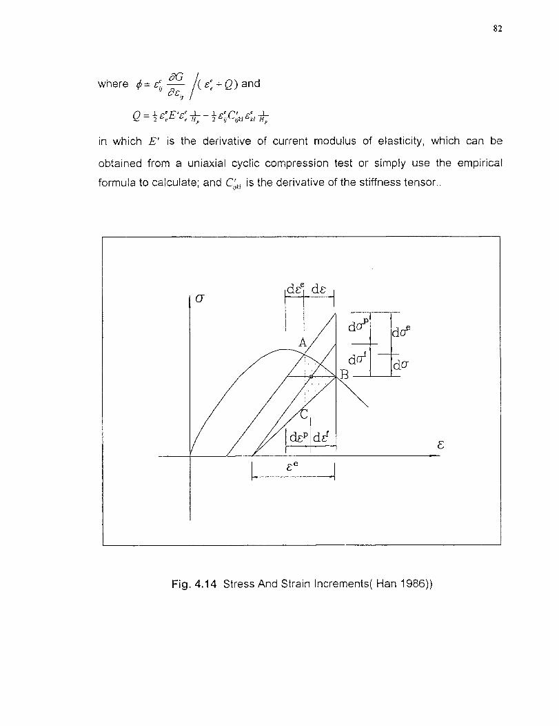
82

where =e` — See + 0) andge,

Q = E -

in which E' is the derivative of current modulus of elasticity, which can be

obtained from a uniaxial cyclic compression test or simply use the empirical

formula to calculate; and Cu'Ai is the derivative of the stiffness tensor..

Fig. 4.14 Stress And Strain Increments( Han 1986))

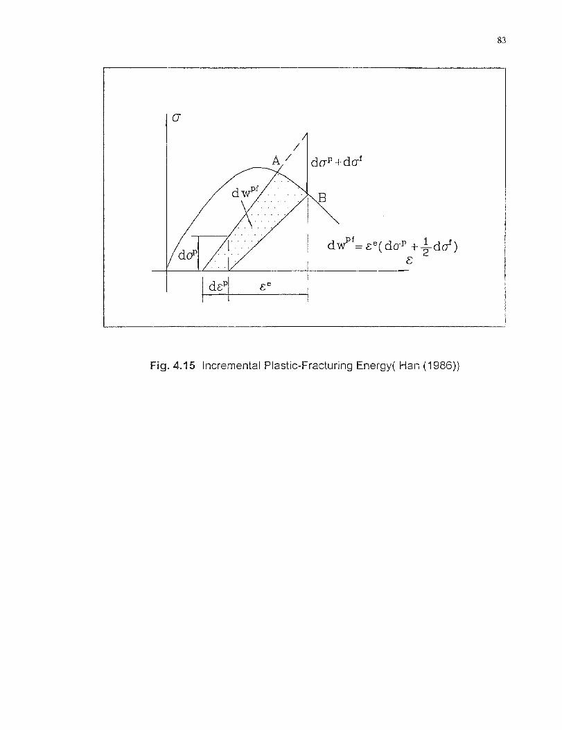
83

Fig. 4.15 Incremental Plastic-Fracturing Energy( Han ( 986))

CHAPTER 5

MODEL PREDICTIONS

5.1 Introduction

The performance of the proposed model must be examined before it can be

used in a finite element analysis program for a structural analysis. When a

structure is subject to external loading, various stress states or strain states

could occur in the structure. A good constitutive model is therefore required to

be usable for all the possible states.

The present model is built up on the strain space. Thus, the basic input is

the strain tensor. Because of the restriction of testing machines and human

habit, most multiaxial experimental data available are from the stress-controlled

tests. Thus, when using the model for predictions, the strain tensor or simply the

three principal strains are needed to be extracted from the experimental data for

each increment. And the comparison will be performed on the stresses. The

input file requires the following information:

(1) Input the most basic material properties, such as the modulus of elasticity

E, the poisson's ratio ii, and the uniaxial compressive strength f:.

(2) Determine the four-parameter critical surface by the approach given in

Chapter 3.

(3) Determine the relationship between the hydrostatic strain of the uniaxial

case and the hardening parameter , that is, p1(k0).

(4) Determine the constants A, p, pc , k and lc, for the loading functions.

(5) Choose M for the ratio of Kinematic and Non-isotropic hardenings. It is

advised to use 1 before the critical surface, and 0 after the failure surface.

84

85

(6) Obtain the theoretical expression of the uniaxial stress-strain relationship.

The expression is used to derive the plastic stress-strain relation, which is

further used for the calibration of the plastic effective stress-effective

strain curve.

(7) The non-associated flow rule of Drucker-Prager type is adopted in the

program. The factor u changes from initial value, -0.5-0.6 at yield to

0-0.02 at the critical surface, and to 0.15-0.25 at the ultimate strength.

They are dependent upon the strength of concrete and type of loading. A

concrete with lower strength seems to exhibit relatively larger

compaction/dilatation behavior, and the dilatation seems to be larger in

biaxial compression loadings than in triaxial compression cases. A simple

choice can be made based on this.

5.2 Stiffness Matrix Col in Strain Softening

5.2.1 Degradation of Stiffness in Uniaxial Case

In Fig. 2.5, the stiffness degradation can be seen from the slope decrease of the

dashed lines with increasing strain. The change rate could be obtained by a

strain controlled uniaxial cyclic compression test. In general, however, such a

test data is not available. In this situation, the following empirical relationship by

Karsan and Jirsa (1969) can be used to compute the slope-strain relationship

Et (c)

= 0.145 (-61 )2 ± 0.13 (—)

(5.1)

where e is the current strain at unloading point; s is the strain at L' ; and cp is

the residual strain or plastic strain at zero stress.

86

5.2.2 Stiffness Degradation Rate of Tensor

To accurately determine the stiffness degradation rate with 21 components is

difficult or even impossible at the present time, due to lack of good and

comprehensive experimental data. However, under the isotropic assumption,

which is an acceptable approximation in the mixed type failure mode, the elastic

tensor has only two independent constants, the modulus of elasticity E and

poisson's ratio With the current E (e) p(s) and their rates are known, Cul l)

may be expressed in the following equation

- C, C,C„, C, C2 0

C, C, C,C3

0 C3

(5.2)

C3

where

E'(1-,u) 2,u(2-,u)'

(1+ ,u)(1 - 2 p)+ E p (I + ,u) - (1 - 2 p) 2

E' ,u 1+ 2,u 2C, = + Ei/

- (1 + p)(1- 2 p) (1 + p) 2 (1- 2,u) 2

E' EI.11C, =

2(1+p) (1+,0 2

Since the poisson's ratio ,u(E) is not easy to be determined and its range

is also a problem to be studied, for simplicity, it may be chosen as a constant.

87

5.3 Comparison Between Model Prediction and Experimental Results

In this study, comparison of the model predictions have been performed with

three sets of test results.

The most well-known Kupfer's test (Kupfer et al (1969)), is considered

first, which provides stress-strain behavior of concrete under biaxial loadings.

The second set of test data is taken from Liu et al's data (Liu et al (1972)). And

the third is given by Schickert and Winkler (1977). The last set of data include

the proportional loadings as well as non-proportional ones.

5.3.1 Comparison with Kupfer's Test

The four critical surface constants are given in Table 3.1. The other material

constants are in Table 5.1, in which ky, corresponds to a uniaxial compressive

yield stress 0.4f . The uniaxial compressive stress-strain curves have been

given by the test itself, which is used as a material input, and also is used to

compute the relationship p l = p, (k).

Table 5.1 Basic Material Constants of Kupfer et al's Test

E

(MPa)

1-1 .1",'

(MPa)

A Pt

(m/m)

pc

(m/m)

ky kp

31700 0.22 32.8 -4.827 x 10 -4 0 -4.327 x 10 -4 0.262 1.55

Fig. 5.1—Fig.5.3 show the comparison for uniaxial and biaxial

compressive loadings. The predicted curves are in good agreement with the test

data in both softening as well as hardening ranges. Figs. 5.4 and 5.5 discuss the

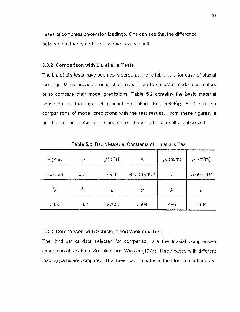
cases of compression-tension loadings. One can see that the difference

between the theory and the test data is very small.

5.3.2 Comparison with Liu et al' s Tests

The Liu et al's tests have been considered as the reliable data for case of biaxial

loadings. Many previous researchers used them to calibrate model parameters

or to compare their model predictions. Table 5.2 contains the basic material

constants as the input of present prediction. Fig. 5.6-Fig. 5.13 are the

comparisons of model predictions with the test results. From these figures, a

good correlation between the model predictions and test results is observed.

Table 5.2 Basic Material Constants of Liu et al's Test

E (Ksi)

2635.94

ky

0.333

f: (Psi) A Pi (rift) pc (m1m)

0.21 4918 -8.333x 10 -5 0 -5.66x 10-4

kp a a fl

1.331 197000 2604 496 6884

5.3.3 Comparison with Schickert and Winkler's Test

The third set of data selected for comparison are the triaxial compressive

experimental results of Schickert and Winkler (1977). Three cases with different

loading paths are compared. The three loading paths in their test are defined as:

88

89

(1) Path 1: Apply hydrostatic loading to 25.5 Mpa. Then keep this value

constant, and load along the compressive meridian, i.e., load on the

deviatoric plane and along (9= 60°.

(2) Path 2: Apply hydrostatic loading to 51 Mpa. Then keep this value

constant and load along the shear meridian, i.e., load on the deviatoric

plane and along 9=30° .

(3) Path 3: Apply hydrostatic loading to 42.5 Mpa. Then keep this value

constant, and load along the tensile meridian, i.e., load on the deviatoric

plane and along 0=0°.

The four critical surface constants are given in Table 3.6. The other

material constants are given in Table 5.3. Fig.5.14 shows the uniaxial

compressive curves. They are in good agreement. Fig .5.15-Fig. 5.17 are for the

triaxial compressive curves. From these figures, one can find that with high

hydrostatic pressures sustained, the predictions are not as good as Fig. 5.14.

But the trend of the predictions is right. Thus, these predictions are acceptable.

Table 5.3 Basic Material Constants of Schickert et al's Test

E 1-1 f: A P, Pc ky kp

(MPa) (MPa) (m/m) (m/m)

21000 0.23 30.6 -8.45x 10-4 0 -3.0x 10 -4 0.44 1.40

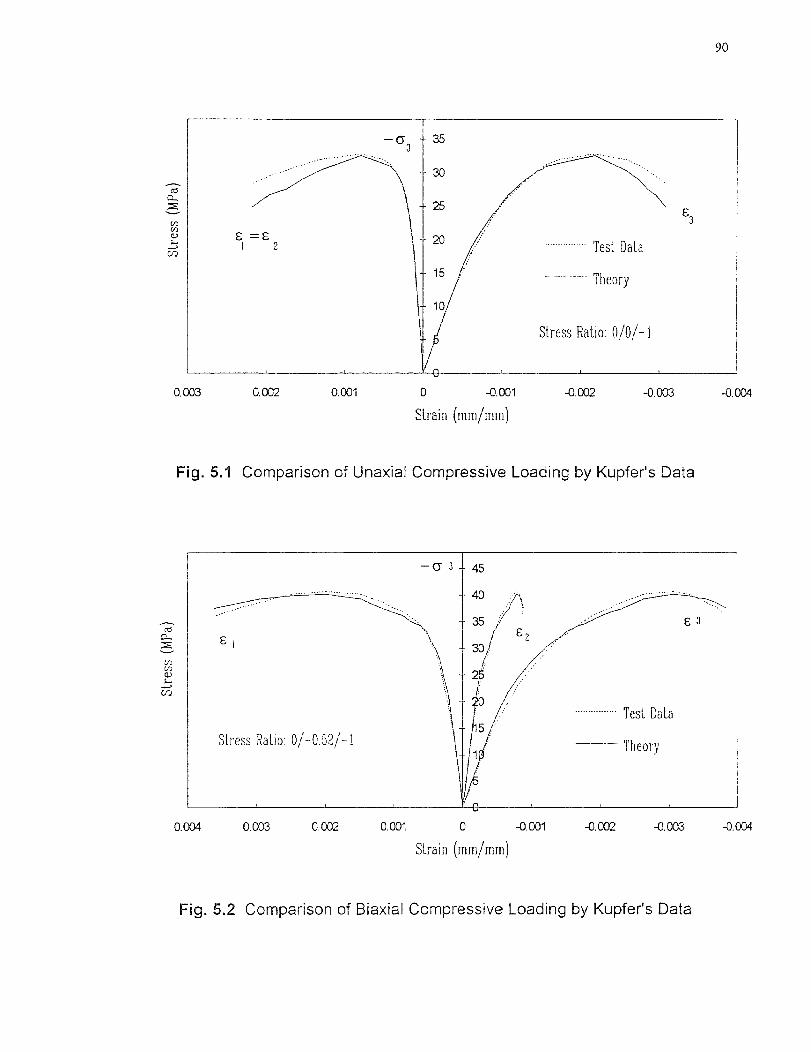
-0.0010Strain (mm/mm)

90

Stress Ratio: 0/0/-1

0.0010.0020.003 -0.004-0.002 -0.003

-0.0010.001 0

Strain (mm/mm

Stress Ratio: 0/-0.52/-1

-0.002 -0.003 -0.0040.0020.0030.004

Fig. 5.1 Comparison of Unaxial Compressive Loading by Kupfer's Data

Fig. 5.2 Comparison of Biaxial Compressive Loading by Kupfer's Data

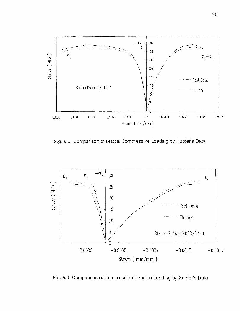
Stress Ratio: D/-1/-1

3

0

0.005 a 004 0.003 0.002 0.001 0 -0.001 -0.002 -0.003 -0.004

Strain mm/mm )

Test Data

Theory

Theory

Stress Ratio: 0.052/0/-1

0.0003 -0.0007

Strain ( mm/mm )

-0.0012 -0.0017

91

Fig. 5.3 Comparison of Biaxial Compressive Loading by Kupfer's Data

Fig. 5.4 Comparison of Compression-Tension Loading by Kupfer's Data

Test Data

Theory

Stress Ratio: 0.103/0/-1

- 25

92

E

0.0004 0.0002 0 -0.0002 -0.0004 -0.0006 -0.0008 -0.001

Strain ( rnm/rnm )

cr.)C.%

U)

Fig. 5.5 Comparison of Compression-Tension Loading by Kupfer's Data

6000— a

5000

E1 E 4000 83

300D Test Data

2000 Theory

1 000 Stress Ratio: 0/0/-1

0 001 0.0005 -0.0005 -0.001 -0.0015 -0. 0 ,02 -0.0025 -0.003

Strain (in/in)

Fig. 5.6 Comparison of Uniaxial Compressive Loading by Liu et al's Data

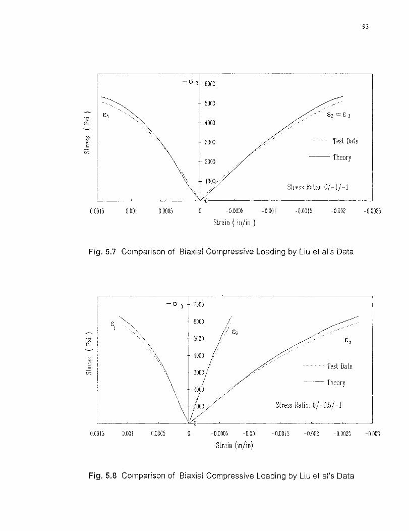
= 3

Test Data

Theory

Stress Ratio: 0/-1/-1

6000

5000

4000

3000

2000

1000 ,

- CY 3

93

E-0

CJ

0.00 th

0.001

0.0005

0 -0.0005 -0.001 -0 0015 -0.002 -0.0025

Strain ( in/in )

Fig. 5.7 Comparison of Biaxial Compressive Loading by Liu et al's Data

0.0015 0.001 0.0005 0 -0.0005 -0.001 -0.0015 -0.002 -0.0025 -0003

Strain (in/in)

Fig. 5.8 Comparison of Biaxial Compressive Loading by Liu et al's Data

82=E3- 500

Stress Ratio: 1/0/0

Test Data

Theory

-0 00010.00005 0

Strain ( in/in )

0.00010 00015 -0 00005

- 500

Stress Ratio: 1/1/0 - 400

- 300

94

0.00016 0.00014 0.00012 0.0001 100008 0.00006 0.00004 0.00002 0 -0.00002 -0.00004

Strain (in/in)

Fig. 5.9 Comparison of Uniaxial Tensile Loading by Liu et al's Data

Fig. 5.10 Comparison of Biaxial Tensile Loading by Liu et al's Data

Test Data

Theory

Stress Ratio: 1/0.5/0

600

500

400

300

200

a 3 4500

24000

3500

3000

2500

2000

1500

1000

500

E

Test Data

Theory

Stress Ratio: 0/0.05/-1

0

95

0 0002

0.00015

0.0001 0.00005

0 -0.00005

Strain (in/in)

Fig. 5.11 Comparison of Biaxial Tensile Loading by Liu et al's Data

0.001

0.0005

0 -0.0005 -0.001 -0.0015 -0 002

Strain (in/in)

Fig. 5.12 Comparison of Compression-Tension Loading by Liu et al's Data

CJ

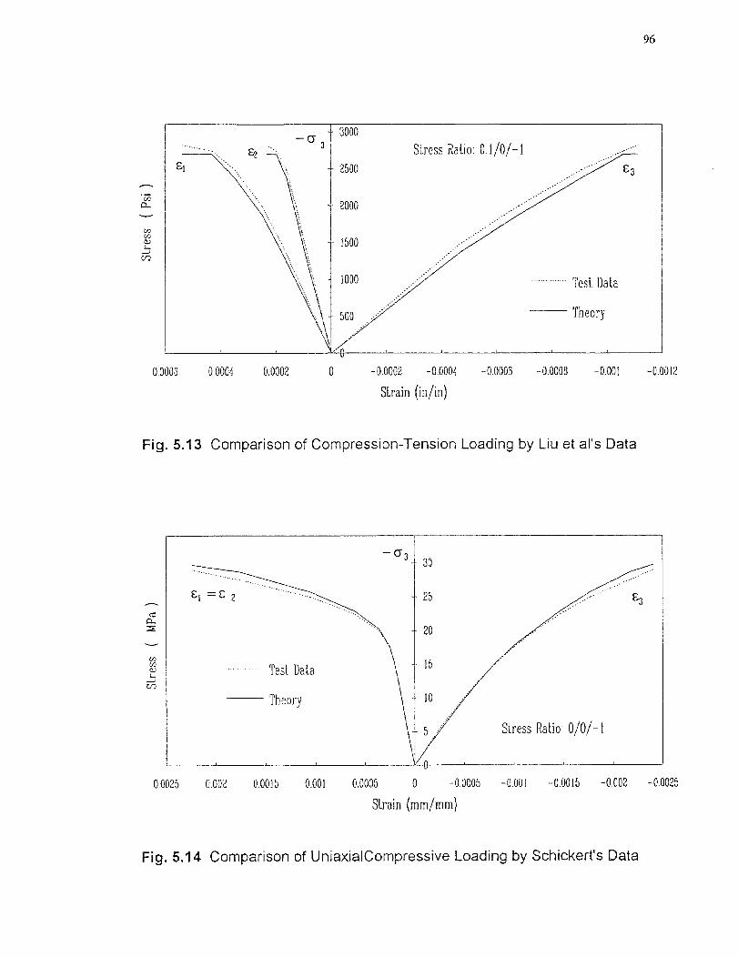
2500

2000

1500

1000

500

Test Data

Stress Ratio: 0.1/0/-1

Theory

—a 3 -t 3000

96

0.0006 0.0004 0.0002 0 -0.0002 -0.0004 -0.0006 -0.0008 -0.001 -0.0012

Strain (in/in)

Fig. 5.13 Comparison of Compression-Tension Loading by Liu et al's Data

— a 3 30

8 t 6 2

25

20

Test Data 15

Theory 10

Stress Ratio: 0/0/-1

0.0025 0.002 0.0015 0.001 0.0005 0 -0.0005 -0.001 -0.0015 -0.002 -0.0025

Strain (mm/mm)

a-.

CD

Fig. 5.14 Comparison of UniaxialCompressive Loading by Schickert's Data

6 ..... ...

80

3 100

Stress Path 2

60

40

Test Data

Theory

97

0.004

0.002

0 -0.002 -0.004 -0.006 -0.008 -0.01

Strain (rnmimm)

Fig. 5.15 Comparison of Nonproportional Loading by Schickert's Data (Path 1)

0.002

0 -0.002 -0.004 -0.006 -0.006 -0.01 -0.012 -0.014

Strain (mm/mm)

Fig. 5.16 Comparison of Nonproportional Loading by Schickert's Data (Path 2)

........... .............. ...........

........... • •-•

6 3

80

70

Stress Path 3

Test Data

Theory

98

0.0025 O{0}5 0.0005 -0.0005 -0.0015 -0.0025

Strain (rnm/rnm)

-0.0035 -0.0045 -0 0055

Fig. 5.17 Comparison of Nonproportional Loading by Schickert's Data (Path 3)

CHAPTER 6

SUMMARY AND CONCLUSIONS

Concrete is a widely used material. Its constitutive relationship has been studied

through many approaches. It is well-known that the plasticity method is an

excellent tool to describe the behavior of concrete. In this study, a relatively

complete constitutive model is developed for concrete in strain space within the

framework of plasticity theory. A critical surface in strain space is set up at the

point of the critical stress. With the critical surface as a reference surface, the

initial and subsequent yield surfaces, including the failure surface, are defined

according to the test results and appropriate assumptions. A modified isotropic

hardening rule and a simple kinematics hardening rule are adopted. A non-

associated flow rule in Drucker and Prager's form is used to account for an

inelastic dilatant behavior of concrete. The working-hardening level is described

by the modified plastic modulus, which is obtained on the basis of the plastic

modulus of a uniaxial compressive plastic stress-strain relationship and a

modification factor of the hydrostatic pressure sensitivity and the dependence of

lode angle. The stiffness degradation in the post-peak range is accounted for.

The predicted stress-strain curves are found to compare well with the

experimental data. Based on the results and observations, the following

conclusions can be made.

(1) The strain-space plasticity theory can be used to model concrete behavior

in both strain-hardening and strain softening. The strain-space

formulation overcomes the difficulties encountered in the application of

stress-space formulation to strain-softening modeling.

99

100

(2) It is reasonable to use a continuum theory to discuss the strain softening

of concrete under the mixed failure, in which the microcracks or fractures

are generally not strongly oriented but may distribute randomly.

(3) The behavior of plastic deformation coupled with an elastic degradation is

observed for concrete materials in the post-peak range. It is logical and

practical to combine the concept of fracturing theory into the plasticity

theory.

(4) Since very limited experimental data is available about strain state of

concrete, little and incomplete information of the strain state behavior is

known. It is impossible to set up a model depending completely on the

test result. In other words, appropriate assumptions on the basis of

qualitative results need to be made in determining the yield surface,

hardening rule, and flow rule. In this situation, a simple and clear model is

practical and preferable. In this model, the loading surfaces at different

stages are defined on the limited test data together with reasonable

assumptions. Results show that this is a good and effective approach.

(5) The most important inelastic behaviors of concrete have been

represented by this model, including brittle failure in tension, ductile

behavior in compression, hydrostatic sensitivities, and volumetric dilation

under compressive loadings.

(6) The model provides rooms and flexibilities to fit wide range experimental

data. The parameters used are shape factor k , the plastic modulus

modification factor, Al(ps ,0), and the dilation factor W. can further be

adjusted and calibrated on the basis of experimental data. As the broad

data become available and the detailed behavior of concrete becomes

known, this model can be further improved.

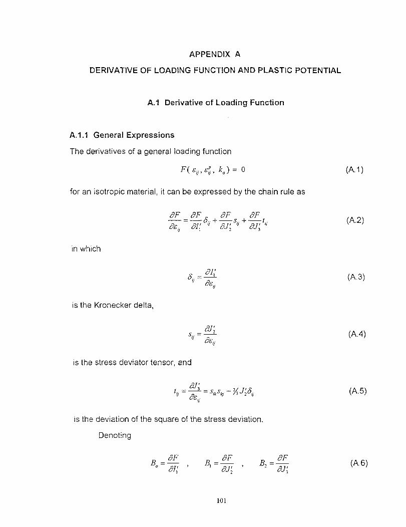
APPENDIX A

DERIVATIVE OF LOADING FUNCTION AND PLASTIC POTENTIAL

A.1 Derivative of Loading Function

A.1.1 General Expressions

The derivatives of a general loading function

ko ) = 0 (Al)

for an isotropic material, it can be expressed by the chain rule as

OF OF OF OFos

=Oil" 0,12° r1 0.1;

(A.2)

in which

is the Kronecker delta,

is the stress deviator tensor, and

(A.3)

(A.4)

.7/3 1;(50. (A.5)

is the deviation of the square of the stress deviation.

Denoting

OF OF OFB° = Bi= B, (A 6)

101

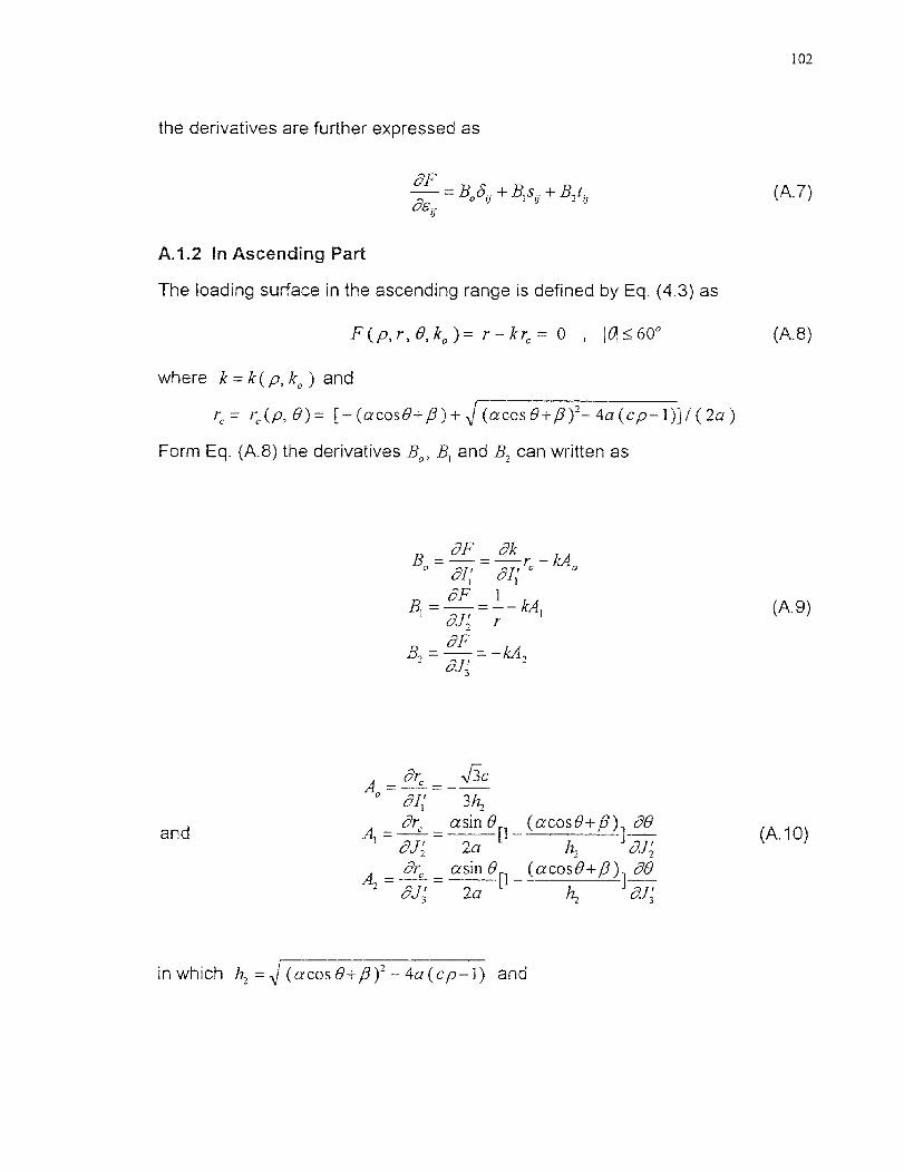
the derivatives are further expressed as

102

SF-B5.+Bs.+Bi0 1.1 2 (A.7)

&v.

A.1.2 In Ascending Part

The loading surface in the ascending range is defined by Eq. (4.3) as

F(p,r,9,k0 )= r - kr,= 0 , 60°

where k k(,o,ko ) and

r = rc (p, 9)= [- (acos8+ 13)+ (acos 8+,3)2- 4a (c p-1)]1 (2a)

Form Eq. (A 8) the derivatives Bo , B, and B, can written as

(A.8)

_ OF _ OkLc, - _ 7.0 - kA 0

OF 1 = kA

rOF

B2 .= = kA 2

(A.9)

and

Or, -■hcAa = =

3h2

AOr, asin 0

E 1 (acos0+P) ] SO

, ---= =OJ; 2a h2 0,112

A-2"Or, asin B P (acost 9 + ,8)

] "SO

5J; 2a h2

(A.10)

in which h, (acos 8+,6)2-4a p-1) and

103

09 3, • J;O`X 4sin 30 1 .0

-N5 1

01; 2 sin 3 J.;%

(A.11)

A.1.3 In Descending Part

The loading function is defined by Eq. (4.10) as

F (p,r ) 0,k0 )= r — ro = 0 lt60° (A 12)

where ro = [7(k o )—c p]l(a l cos0+ Pi ) .

From Eq. (A.12), one has

where

B= =—A° °

OFB = 1 A' a,r2 r

B,= OF = A2- 01;

(A 13)

A = Or,

° 01,' 3(a, cos0+,8, )A Oro = [7(10— cp] a, sin 61 00 ' ei; (a l coso+ ,81 )2 jr

A er,, [7(k c )— cp] a, sin 0 00 2 01; (a, cost9+/3 1 ) 2 0J;

ee in which and are represented by Eq. (A.11).ef; eJ;

(A.14)

104

A.1.4 Derivative at 9= 60 °It should be noted that the term sin 3 a in Eq. (A.11) would go to zero if 0

approaches to 60° , and the derivatives at 60° would be infinite. This is because

there are three corners in the deviatoric sections where there do not exist

derivatives. To treat such singularity, one can simply assume that

= 0 0= 60 °c co s0)

and hence in Eqs. (A.9) and (A.13)

(A.15)

= 0

A, = 0, 0= 60 ° (A.16)

This implies that the normal vector of the failure curve at 9= 60 ° coincides with

the radial direction, which is independent of 0.

A.2 Derivative of Plastic Potential Function

The derivative of the plastic potential function G can be expressed in the form of

tensor invariants as

OG OG OG OG = jai + s,. + t i .

OE.. Of,' OJ OJ;(A.17)

In this research, The Drucker-Prager type of plastic potential function is used

(Eq.(4 31)), thus the derivative can be simplied as

(A.18)

Form elastic matrix Form plastic-fracturing matrix

Calculate strain increment

Crushing ocracking?

YV

Calculate elastic Strain Increment

VScale back to yied surface

\IvForm elastoplastic matrix

Calculate strain increment

Update hardening parameter

N

Update elastic stiffness matrix

VSet stress equal to zero

Update stress and strain

VUpdate stiffness matrix

N

Scale back to failure surface

Crushing ocracking ?

N

105

APPENDIX BFLOW CHART OF MATERIAL SUBROUTINE

CStarD

REFERENCES

Ahmed, S. H. (1981). "Complete Triaxial Stress-Strain Curves for Concrete." Ph.D Dissertation in University of Illinois at Chicago.

Argyris, J. H., Faust, G., Szimmat, J., Warnke, E. P., and Wiliam, K. J.(1974)."Recent Development in the Finite Element Analysis ofPrestressed Concrete Reactor Vessels." Nuclear Engineering and Design,28(1), 42-75.

Argyris, J. H., Faust, G., and Wiliam, K. J. (1976)." Limit Load Anasis of Thick-Walled Concrete Structures-A Finite Element Approach to Fracture."Computer Method in Applied Mechanics and Engineering, Vol. 8, North-Holland Co. 215-243.

Bazant, Z. P. (1971). Discussion of "Triaxial State of Stress of ConcreteStructures," by L. Janda. International Conference on StructuralMechanics in Rector Technology, Berlin, 22.

Bazant, Z. P. and Bhat, P. D. (1976). "Endochronic Theory of Inelasticity andFailure of Concrete." Engrg Mech., ASCE, 102(5), 701-722.

Bazant, Z. P. and Kim, S. S. (1979). "Plastic-Fracturing Theory for Concrete."Engrg Mech., ASCE, 105(3), 407-428.

Eazant, Z. P. and Shieh, C. L. (1980). "Hysteric Fracturing Endochronic Theoryfor Concrete." Engrg. Mech., ASCE, 106(6), 929-950.

Buyukorturk, O. (1977). "Nonlinear Analysis of Reinforced Concrete Structures."Computers and Structures, Vol. 7, 149-156.

Buyukorturk, O. (1979). "A Constitutive Model for Concrete in Compression."Proceedings of the Third ASCE Engrg. Mech. Div. Specialty Conference,Austin, Texas

Carino, N. J. (1976). "Limitation Tensile Strain Criterion for Failure of Concrete."ACI Journal, 73(3), 160-165.

Casey, J. and Naghdi, P. M. (1981). "On the Characterization of Strain-Hardening in Plasticity." J. of Applied Mechanics, Transactions of theASME, 48(2), 285-295.

Casey, J. and Naghdi, P. M. (1983a). Remark on the Definition of Hardening,Softening and Perfectly Plastic Behavior." Acta Mechanica, Vol. 48, 91-94

106

107

Casey, J. and Naghdi, P. M. (1983b). "On the Nonequivalence of the StressSpace and Strain Space Formulations of Plasticity Theory.' J. of AppliedMechanics, Transaction of ASME. 50(2), 3540-35.

Cedolin, L, Crutzen, Y. R. J. and Dei Poli, S. (1977). "Triaxial Stress-StrainRelationship for Concrete." Engrg. Mech., ASCE, 103(3), 423-439.

Chen, A. C. T. and Chen, W. F. (1975). "Constitutive Relations for Concrete."Engrg Mech., ASCE, 101(4), 465-481.

Chen, E. Y. T. and Schnobrich, W. C. (1981). "Material Modeling of PlainConcrete." Advanced Mechanics of Reinforced Concrete, IABSEColloquium, Delft, the Netherlands, 33-51.

Chen, W. F. (1982). Plasticity in Reinforced Concrete. McGraw-Hill Inc.

Dafalias, Y. F. (1977a). "Elasto-Plastic Coupling within Thermodynamic StrainSpace Formulation of Plasticity." International Journal of NonlinearMechanics, Vol. 12, 327-337.

Dafalias, Y. F. (1977b). "Il'iushin's Postulate and Resulting ThermodynamicConditions on Elasto-Plastic Coupling." International Journal of Solids andStructures, 13(3), 239-251.

Darwin, D. and Pecknold, D. A. (1974). "Inelastic Model for Cyclic BiaxialLoading of Reinforced Concrete." Civil Engineering Studies SRS, No. 409,University of Illinois at Urbana-Champaign.

Dougill, J. W. (1976). "On Stable Progressively Fracturing Solids." Journal ofApplied Mathematics and Physics(ZAMP), Vol. 27, 423-437.

Dragon, A. and Mroz, Z. (1979). "A Continuum Theory for Plastic-Brittle Behaviorof Rock and Concrete." International Journal of Engineering Science, Vol.17, No. 2, 121-137

Drucker, D. C. (1950). "Some Implications of Work Hardening and IdealPlasticity." Quarterly of Applied Mathematics, 7(4), 411-418.

Ferrara, G., Rossi, R., Rossi, P. P. and Ruggeri, L. (1976). "Dispositive Di ProvaPer L'analisi Sperimentale Del Comportamento Di ConglomeratiCementizi Sottoposti a Stati Triassiali Di Sollecitazione." Presented at the4th Association Italiana Annalisi Sollecitazione Congress, Held at Rome,Italy.

108

Frantziskonis, G. and Desai, C. S. (1987). "Constitutive Model with StrainSoftening." International Journal of Solids and Structures, Vol. 23, No. 6,733-750.

Gerstle, K. H. (1980). "Behavior of Concrete under Multiaxial Stress States."Engrg. Mech., ASCE, 106(6), 1383-1403.

Gerstle, K. H. (1981). "Simple Formulation of Biaxial Concrete Behavior." ACIJournal, 78(1), 62-68.

Green, S. J. and Swanson, S. R. (1973). "Static Constitutive Relations forConcrete." Technical Report No. AFW-TR-72-244 (AD761820), Air ForceWeapons Lab, New Mexico.

Han, D. J. and Chen, W. F. (1985). "A Nonuniform Hardening Plasticity Modelfor Concrete Materials." Journal of Mechanics of Materials, Vol. 4, 283-302.

Han, D. J. and Chen, W. F. (1986). "Strain-Space Plasticity Formulation forHardening-Softening Materials with Elasto-Plastic Coupling." InternationalJournal of Solid and Structures, 22(8), 935-950.

Han, D. J. and Chen, W. F. (1987). "Constitutive Modeling in Analysis ofConcrete Structures." Engrg. Mech., ASCE, 113(4), 577-593.

Hobbs, D. W. (1974). "Strength and Deformation Properties of Plain ConcreteSubjected to Combined Stress." Part 3, Technical Report 42, Cement andConcrete Association, London, England.

Hsieh, S. S., Ting, E. C., and Chen, W. F. (1982). "A Plasticity Fracture Modelfor Concrete." International Journal of Solids and Structures, 18(3), 181-1 97.

Hsu, C.T.T.(1972). Discussion of "Stress-Strain Response and Fracture ofConcrete in Uniaxial and Biaxial Compression," by Liu, T.C.Y. et al. ACIJournal, 69(11), 711-712.

ll'iushin, A. A. (1961). "on the Postulate of Plasticity." PMM, 25(3), 503-507 (746-752 in English Translation Edition).

Jiang, L., Huang, D. and Xie, N. (1991). "Behavior of Concrete Under TriaxialCompressive-Compressive-Tensile Stresses." AC1 Materials Journal,88(2), 181-185.

109

Kachanov, L. M. (1958). "Time of Rupture Process under Creep Conditions."Izvestia Aksdemii Nauk, USSR, 8 (in Russian), 26-31.

Karsan, P. and Jirsan, J. 0. (1969). " Behavior of Concrete Under CompressiveLoading." Struct. Div., ASCE, 95(12), 2543-2563.

Kotsovos, M. D. and Newman, J. B. (1977). "Behavior of Concrete UnderMultiaxial Stress." ACI Journal, 74(6), 443-446.

Kotsovos, M. D. and Newman, J. B. (1978). "Generalized Stress-Strain Relationsfor Concrete." Energ. Mech., ASCE, 104(4), 845-856.

Kotsovos, M. D. (1979). "Effect of Stress Path on the Behavior of Concrete underTriaxial Stress States." ACI Journal, 76(2), 213-223.

Krajcinovic, D. and Fonseka (1981). "The Continuous Damage Theory of BrittleMaterials." Journal of Applied Mechanics, Vol. 48, No. 4, 809-815.

Krajcinovic, D. (1985). "Constitutive Theories for Solids with DefectiveMicrostructure." Damage Mechanics and Continuum Modeling, N. Stubbsand D. Krajcinovic eds. ASCE, 39-56.

Kupfer, H. and Hilsodorf, H. K. (1969). "Behavior of Concrete Under BiaxialStresses." ACI Journal, 66(8), 656-666.

,pfer, H. and Gerstle, K. H. (1973). "Behavior of Concrete under BiaxialStresses." Engrg. Mech., ASCE, 99(4), 853-866.

Launay, P. and Gachon, H (1971). "Strain and Ultimate Strength of ConcreteUnder Triaxial Stresses." Special Publication, SP-34, AC!, 269-282.

Liu, T. C. Y., Nilson, A. H., and Slate, F. 0. (1972). "Stress-Strain Response andFracture of Concrete in Uniaxial and Biaxial Compression." AC! Journal,69(5), 1025-1034.

Loland. K. E. (1980). "Continuous Damage Model for Load Response Estimationof Concrete." Cement and Concrete Research, 10(3), 495-402.

Lubliner, J., Oliver, J.,011er, S. and Onate, E. (1989). "A Plastic-Damage Modelfor Concrete." International Journal of Solids and Structures, 25(3), 299-326.

Mazars, I. (1981). "Mechanical Damage and Fracture of Concrete Structure."Advances in Fracture Research, 5th International Conference onFracture, 0. Francois, ed.

110

Mizuno, E. and Shigemitsu, H. (1992). "Compressive Softening Model forConcrete." Energ. Mech., ASCE, 118(8), 1546-1563.

Naghdi, P. M. and Trapp, J. A. (1975). "the Significance of Formulating PlasticityTheory with Reference to Loading Surfaces in Strain Space." InternationalJournal of Engineering Science, Vol. 13, 785-797.

Nelissen, L. J. M. (1972). "Biaxial Testing of Normal Concrete." Heron(Delft),18(1), 1-90.

Newman, S. B. and Newman, K. (1972). "The Cracking and Failure of ConcreteUnder Combined Stresses and its implications for Structural Design."RILEM-Symposium on the Deformation and Rupture of Solids Subjectedto Multiaxial Stresses, Part I, Concrete, Cannes, 1972, Paper I/10, 149-168.

Ngo, D., and Scordelis, A. C. (1976). "Finite Element Analysis of ReinforcedConcrete Beam." AC! Journal, 64(3), 152-163.

Ortiz, M. (1985). "A Constitutive Theory for the Inelastic Behavior of Concrete."Mechanics of Materials, 4(1).

Ottosen, N. S. (1977). "A Failure Criterion for Concrete." Engrg. Mech., ASCE,103(4), 527-536.

Ottosen, N. S. (1979). "Constitutive Model for Short-Time Loading of Concrete."Engrg. Mech. ASCE, 105(1), 127-141.

Palaniswamy, R. and Shah, S. P. (1974). "Fracture and Stress-StrainRelationship of Concrete under Triaxial Compression." Struct. Engrg.,ASCE, 100(5), 901-916.

Pekau, O. A., Zhang, Z. X. and Liu, G. T. (1992). "Constitutive Model forConcrete in Strain Space." Engrg. Mech., ASCE, 118(9), 1907-1927.

Peterson, P. E. (1981). "Crack Growth and Development of Fracture Zone inPlain Concrete and Similar Materials," Division of Building Materials, LundInstitute of Technology, Lund, Sweden.

Pietruszczak, S., Jiang, J. and Mirza, F. A. (1988). "An Elastoplastic ConstitutiveModel for Concrete." International Journal of Solids and Structures, 24(7),705-722.

111

Resende, L. (1987). "A Damage Mechanics Constitutive Theory for InelasticBehavior of Concrete." Conput. Methods App!., Mech. Engrg., 60(1), 57-93.

Richart, F. E., Brandtzaeg, A. and Brown, R. L. (1929). "The Failure of Plain andSpirally Reinforced Concrete in Compression." University of IllinoisBulletin, Vol. XXVI, No. 31.

Schickert, G. and Winkler, W. (1977). "Results of Test Concerning Strength andStrain of Concrete Subjected to Multiaxial Compressive Stress." VertriekDurch Verlag Wilhelm Ernst and Sohngk Berlin-Munchen-Dusselvorf.

Schickert, G. and Danssmann, J. (1984). "Behavior of Concrete Stressed byHigh Hydrostatic Compression." RILEM-CEB-CNRS, Int. Conf. onConcrete under Multi-Conditions, Toulouse, 69-84.

Shah, S. P. and Chandra, S. (1968). "Critical Stress, Volume Change andMicrocracking of Concrete." AC! Journal, 65(5), 770-781.

Simo, J. C. and Ju, J. W. (1987). " Strain and Stress Based Continuum DamageModels." Part 1: Formulation, International Journal of Solids andStructures, 23(7), 821-840.

Sinha, B. P., Gerstal, K. H. and Tulin, L. G. (1964). "Stress-Strain Relation forConcrete Under Cyclic Loading." AC! Journal, 61(2), 195-211.

Suidan, M. and Schnobrich, W. C. (1973). "Finite Element Analysis ofReinforced Concrete." Struct. Engrg., ASCE, 99(10), 2109-2122.

Tasuji, M. E., Slate, F. 0., and Nilson, A. H. (1978). "Stress-Strain Responseand Fracture of Concrete in Biaxial Loading." AC1 Journal, 75(7), 306-312.

Torrent, R. J., Dvorkin, E. N., and Alvaredo, A. M. (1987). "A Model for Work-hardening Plasticity and Failure of Concrete under Multiaxial Stress."Cement and Concrete Research, Vol. 17, 939-950.

Valanis, K. C. (1971). "A Theory of Viscoelasticity without a Yield Surface."Archiwum Mechaniki Stossowarej (Archives of Mechanics, Warsaw), Vol.23, 517-551.

Wastiels, J. (1979). "Behavior of Concrete under Multiaxial Stresses--- Areview." Cement Concrete Research, 9(1), 35-44.

112

Wiliam, K. J. and Warnke, E. P. (1974). "Constitutive Model for the TriaxialBehavior of Concrete." Presented at the 1974 International Association forBridge and Structural Engineering Seminar on Concrete StructuresSubjected to Triaxial Stresses, Held at Bergamo, Italy.

Yazdani, S. and Schreyer, H. L. (1990). "Combined Plasticity and DamageMechanics Model for Plain Concrete." Engrg. Mech., ASCE, 116(7), 1435-1451.

Yoder, P. J. and Iwan, W. D. (1981). "On the Formulation of Strain-spacePlasticity With Multiple Loading Surfaces." J. of Applied Mechanics,ASME, 48(4), 773-778.