Embed Size (px)
Citation preview

Inf. Sci. Lett. 2, 1, 35-47 (2013) 35
Rough Sets Theory as Symbolic Data Mining Method: An Application on
Complete Decision Table
Mert Bal
Mathematical Engineering Department, Yildiz Technical University, Esenler, İstanbul, TURKEY
E-mail: [email protected] Received: 21 May 2012; Revised 25 Nov. 2012; Accepted 27 Nov. 2012
Abstract: In this study, the mathematical principles of rough sets theory are explained and a sample application
about rule discovery from a decision table by using different algorithms in rough sets theory is presented.
Keywords: Rough Sets Theory, Data Mining, Complete Decision Table, Rule Discovery
1. Introduction
Data mining and usage of the useful patterns that reside in the databases have become a very
important research area because of the rapid developments in both computer hardware and
software industries. In parallel with the rapid increase in the data stored in the databases,
effective use of the data is becoming a problem. To discover the rules or interesting and useful
patterns from these stored data, data mining techniques are used. If data is incomplete or
inaccurate, the results extracted from the database during the data discovery phase would be
inconsistent and meaningless. Rough sets theory is a new mathematical approach used in the
intelligent data analysis and data mining if data is uncertain or incomplete. This approach is of
great importance in cognitive science and artificial intelligence, especially in machine
learning, decision analysis, expert systems and inductive reasoning.
There are many advantages of rough set approach in intelligent data analysis. Some of these
advantages are being suitable for parallel processing, finding minimal data sets, supplying
effective algorithms to discover hidden patterns in data, valuation of the meaningfulness of
the data, producing decision rule set from data, being easy to understand and the results
obtained can be interpreted clearly. In the last years, rough sets theory is widely used in
different areas like engineering, banking and finance.
In the last decades, the size of the data stored in the databases of the organizations has been
growing each day and therefore we face difficulties about obtaining the valuable data.
Databases are a collection of relational and non-recurring data to meet the demands of the
organizations. Because the data stored in the databases is growing each day, it is getting
harder for the users to reach the accurate and useful information. In the last few years,
because of the rapid developments in both computer hardware and software industries, the
increase in the storage capacities of huge databases, the data mining and the usage of the
useful patterns that reside in the databases, became a very important research area. To
discover the rules or interesting and useful patterns among these stored data in the databases,
data mining techniques are used. Storing huge amount of increasing data in the databases,
which is called information explosion, it is necessary to transform these data into necessary
and useful information. Using conventional statistics techniques fail to satisfy the
Information Science Letters An International Journal
An International Journal © 2012 NSP
@ 2013 NSP
Natural Sciences Publishing
Cor.

36 Mert BAL: Rough Sets Theory as Symbolic Data Mining ......
requirements for analyzing the data, in the last years, the newly developed concepts Data
Mining and Knowledge Discovery in Databases are getting more important.
One of the approaches used in data mining and knowledge discovery is rough sets theory.
According to this method, which is proposed in the beginning of 1980’s, it is thought that
knowledge can be obtained from every object in the universe.
In this study, the mathematical principles of rough sets theory are explained and a sample
application about rule discovery from a decision table by using different algorithms in rough
sets theory is presented.
2. Data Mining and Knowledge Discovery in Databases
Data Mining is a discovery process of the hidden information from data which is yet unknown
and potentially useful. On the other hand, according to Raghavan and Sever, data mining
discovers the general patterns and relations hidden in the data (Sever and Oguz, 2003).
Decision rules are one of the widely used techniques to present the obtained information. A
decision rule summarizes the relation between the properties. To transform the raw data
residing in the database into valuable information, several stages of data processing is
required. Data Mining is an iterative process that acts as a bridge between logical decision-
making and the data, and is possible the classification for finding the useful samples or using
and combining the classification rules from the samples. This process combines the
approaches used in different disciplines like machine learning, statistics, database
management systems, data warehousing, and constraint programming (Sever and Oguz,
2003).
In recent years many successful machine learning applications have been developed, in
particular in domain of data mining and knowledge discovery. One of common tasks
performed in knowledge discovery is classification. It consists of assigning a decision class
label to a set of unclassified objects described by a fixed set of attributes (features). Learning
algorithms induce various forms of classification knowledge from learning examples, i.e.,
decision trees, rules, Bayesian classifiers. Decision rules are represented as logical
expressions of the following form:
IF (conditions) THEN (decision class)
where conditions are formed as a conjunction of elementary tests on values of attributes. A
number of various algorithms have already been developed to induce such rules.
Decision rules are one of the most popular types of knowledge used in practice; one of the
main reasons for their wide application is their expressive and easily human-readable
representation. (Stefanowski, 2003)
There are many successful applications of data mining process in many different areas. Many
methods to discover the useful patters are available in data mining applications and each
method has advantages and disadvantages over the others. However, when needed, the
advantages of different methods can be combined and hybrid methods may be created. The
process of creating hybrid methods is a work of combining computational intelligence tools.
Many algorithms are used to implement a DM process. The reason is that some technologies
result better than the others for different tasks, states and subjects do. There is a model
creation process that represents a data set in the core of the data mining. A model creation
process that represents a data set is generic for all DM products; on the other hand, the
process itself is not generic.
Some methods used in DM processes are rough sets theory, Bayesian networks, genetic
algorithms, neural networks, fuzzy sets and inductive logic programming.
DM functions are used to determine the pattern types that may exist in the DM tasks.
Generally, DM tasks are classified into two categories as descriptive and estimator.
Descriptive mining tasks characterize the general properties of data in the database. On the

Mert BAL: Rough Sets Theory as Symbolic Data Mining ...... 37
other hand, estimator mining makes inferences from the available data to make predictions
(Han and Kamber, 2001). The samples of the DM functions and resulting discovered pattern
types are classification, clustering, summarization, estimation, time series analysis,
association rules, sequence analysis and visualization.
3. Rough Sets Theory
Rough sets theory is proposed by (Pawlak, 1982) in the beginning of 1980’s and it is based on
the assumption that knowledge can be obtained from each object in the universe (Nguyen and
Slezak, 1999, Pawlak, 2002).
In rough sets theory, the objects, characterized by the same information, have the same
existing knowledge; this means they are indiscernible. Indiscernibility relationship produced
using this way forms the mathematical basis of the rough sets theory. The sets of the same
indiscernible objects are called “elementary set” and form the smallest building blocks
(atoms) of the information about the universe. Some combinations of those elementary sets
are called “crisp set”, otherwise the set is called “rough set” Each rough set has boundary
region. For example, like the unclassified objects with certainty. Significantly, rough sets, in
contrast precise sets, cannot be characterized by the information of their elements. A rough set
and a precise set pair are called the lower and upper approximation of the related rough set.
Lower approximation contains all the objects belong to the set but upper approximation
contains the objects that may belong to the set. The differences between these lower and
upper approximations define the boundary region of the rough set. The lower and the upper
approaches are two basic functions in the rough sets theory.
There are many advantages of the rough sets approach in data analysis. Some of them are as
follows:
It finds minimal data sets and generates a decision rule from the resulting data.
It performs the clear interpretations of the results and evaluation of the meaningfulness
of the data.
Many algorithms based on rough sets theory in particular are suitable for parallel
processing (Pawlak, 2002).
Non-linear or discontinuous functional relations modeling capability supplies a strong
method that can qualify the multi-dimensional and complex patterns. Because
generated rules and used properties are not excessive, the patterns are concise, strong
and sturdy. In addition, it supplies effective algorithms to find the hidden patterns in
the data.
Rough sets can identify and characterize the uncertain systems.
Because the rough sets show the information as easy to understand logic patterns,
where the inspection and validity of the data required or the decisions are taken by the
rules and suitable for the supported situations, this method is successful (Binay, 2002).
The basic concepts of rough set theory will be explained below.
3.1. Information Systems
In rough sets theory, a data set is represented as a table and each row represents a state, an
event or simply an object. Each column represents a measurable property for an object (a
variable, an observation, etc.). This table is called an information system. More formally, the
pair A,U represents an information system. U is a finite nonempty set that is called
universe and A is a finite nonempty set of properties. Here, for Aa , aVUa : . The set
aV is called the value set of a . Another form of information systems is called decision

38 Mert BAL: Rough Sets Theory as Symbolic Data Mining ......
systems. A decision system (i.e., decision table) expresses all the knowledge about the model.
A decision system is dU A, form of any information system. Here, Ad are
decision attributes. Other attributes da A are called conditional attributes. Decision
attributes can have many values, but usually they have a binary value like True or False
(Komorowski, et.al., 1998, Hui, 2002). Decision system and decision rule will be explained in
details in Section 4.
3.2. Indiscernibility
Decision systems, which are a special form of information systems, contain all information
about a model (event, state). In decision systems, the same or indiscernible objects might be
represented more than once or the attributes may be too many. In this case, the result table
will be larger than desired. The relation about indiscernibility is as follows:
If a pair of relation XXR is either reflective (if an object relates to itself xRx ),
symmetrical (if xRy then yRx ) or transitive (if xRy and yRz then xRz ) then it is an
equivalence relation. The equivalence class of Xx element contains all Xy objects,
where xRy . Provided that A,U is an information system, then there is an equivalence
relation between any AB and a BIND :
yaxBaaUyxBIND |, 2 (1)
BIND , B is called indiscernibility relation. If BINDyx , , then the objects x and y
are indiscernible with the attributes in B . The equivalence class of indiscernibility relation
B is represented by Bx (Komorowski, et.al., 1998, Komorowski et.al., 1999). The
indiscernibility relation BIND separates a universal set U , given as a pair of equivalence
relation, into an rXXX .,,........., 21 equivalence classes family. All equivalence classes
family rXXX .,,........., 21 defined by the relation BIND in set U forms a partition of set
U and it is represented by B . The equivalence classes family
B is called classification and
represented by the expression BINDU / . The objects belonging to the same equivalence
classes iX are indiscernible; otherwise, the objects are discernible by attributes subset B . The
equivalence classes iX , r.,,.........2,1 of BIND relation are called elementary sets B in an
information system .
Bx shows an elementary set B containing the element x and it is defined by the following
equation (2):
yxINDUyx B | (2)
A sequenced pair BINDU , is called approximation space. Any finite combination of
elementary sets in an approximation space is called a set defined in the approximation space
(Binay, 2002). A elementary sets of an information system A,U are called the atoms
of information system .
3.3. Discernibility Matrix
The study on the indiscernibility of the objects is carried out by Skowron and Rauszer (1992).
In this study, indiscernibility function and indiscernibility matrix related to the creation of
efficient algorithms for creating minimal feature subsystems sufficient to define all the
aspects in a given information system are presented.
Let us assume that is an information system that contains n number of objects. The
indiscernibility matrix M for the information system is a nn symmetrical matrix,
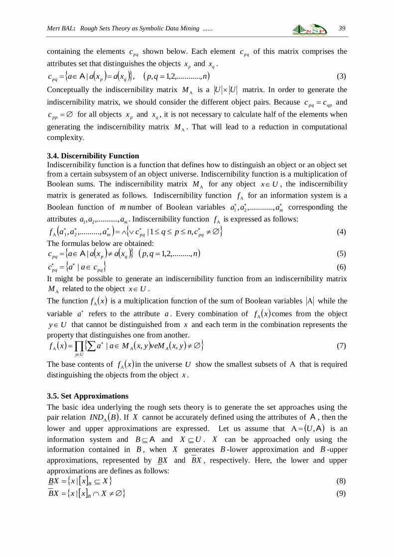
Mert BAL: Rough Sets Theory as Symbolic Data Mining ...... 39
containing the elements pqc shown below. Each element pqc of this matrix comprises the
attributes set that distinguishes the objects px and
qx .
qppq xaxaac |A , nqp ...,,.........2,1, (3)
Conceptually the indiscernibility matrix M is a UU matrix. In order to generate the
indiscernibility matrix, we should consider the different object pairs. Because qppq cc and
ppc for all objects px and qx , it is not necessary to calculate half of the elements when
generating the indiscernibility matrix M . That will lead to a reduction in computational
complexity.
3.4. Discernibility Function
Indiscernibility function is a function that defines how to distinguish an object or an object set
from a certain subsystem of an object universe. Indiscernibility function is a multiplication of
Boolean sums. The indiscernibility matrix M for any object Ux , the indiscernibility
matrix is generated as follows. Indiscernibility function f for an information system is a
Boolean function of m number of Boolean variables
maaa ...,,........., 21 corresponding the
attributes maaa ..,,........., 21 . Indiscernibility function f is expressed as follows:
pqpqm cnpqcaaaf ,1|.,,........., 21 (4)
The formulas below are obtained:
qppq xaxaac |A nqp ,,.........2,1, (5)
pqpq caac | (6)
It might be possible to generate an indiscernibility function from an indiscernibility matrix
M related to the object Ux .
The function xf is a multiplication function of the sum of Boolean variables while the
variable a refers to the attribute a . Every combination of xf comes from the object
Uy that cannot be distinguished from x and each term in the combination represents the
property that distinguishes one from another.
Uy
AA yxveMyxMaaxf ,,| (7)
The base contents of xf in the universe U show the smallest subsets of that is required
distinguishing the objects from the object x .
3.5. Set Approximations
The basic idea underlying the rough sets theory is to generate the set approaches using the
pair relation BIND . If X cannot be accurately defined using the attributes of A , then the
lower and upper approximations are expressed. Let us assume that A,U is an
information system and AB and UX . X can be approached only using the
information contained in B , when X generates B -lower approximation and B -upper
approximations, represented by XB and XB , respectively. Here, the lower and upper
approximations are defines as follows:
XxxXB B | (8)
XxxXB B| (9)

40 Mert BAL: Rough Sets Theory as Symbolic Data Mining ......
The objects in XB , B are classified certain members of X on the base of the information
contained in B .The objects in XB can be classified probable members of X on the base of
the information contained in B .
XBXBXBN B (10)
The equation (10) is called B -boundary region of X , and then it comprises the objects that
cannot be classified certainly members of X on the base of the information contained in B .
The set XBU is called B -outside region of X , and it comprises the objects that certainly
not belong to X on the base of the information contained in B .
If XBXBXBN B, which is XBXB , the set B is called certain set.
XBXBXBN B If XBXB , then the set B is called rough set. In this case, the set
B can be qualified only with lower and upper approximations. Figure 1 shows the upper and
lower approximations of set X .
Figure 1. Upper and lower approximations of set X
The lower and upper approximations have the properties that are shown below:
XBXXB (11)
BB , UUBUB (12)
YBXBYXB (13)
YBXBYXB (14)
YX implies YBXB and YBXB (15)
YBXBYXB (16)
YBXBYXB (17)
XBXB (18)
XBXB (19)
XBXBBXBB (20)
XBXBBXBB (21)
Here, X means XU .
One can define the following four basic classes of rough sets, i.e., four categories of
vagueness:
a) X is roughly B -definable, iff XB and UXB .
b) X is internally B -undefinable, iff XB and UXB .

Mert BAL: Rough Sets Theory as Symbolic Data Mining ...... 41
c) X is externally B -undefinable, iff XB and UXB .
d) X is totally B -undefinable, XB and UXB .
The intuitive meaning of this classification is the following.
X is roughly B -definable means that with the help of B we are able to decide for some
elements of U that they belong to X and for some elements of U that they belong to - X .
X is internally B -undefinable means that using B we are able to decide for some elements
of U that they belong to - X but we are unable to decide for any element U whether it
belongs to X .
X is externally B -undefinable means that using B we are able to decide for some elements
of U that they belong to X but we are unable to decide for any element U whether it
belongs to - X .
X is totally B -undefinable means that using B we are unable to decide for some element of
U whether it belongs to X or - X (Komorowski et.al., 1998).
The universe can be divided into three disjoint regions using the upper and lower
approximations, relating to any subset UX . Boundary, positive and negative regions are
described as below.
XBXBXBND (22)
XBXPOS (23)
XBUXNEG (24)
A member of the negative region XNEG does not belong to X . A member of the positive
region XPOS belongs to X , and only one member of the boundary region XBND
belongs to X (Allam et.al., 2005). These regions are shown in the Figure 2.
Figure 2. The negative, positive and the boundary regions of a rough set
A rough set X can be characterized numerically with the following coefficient:
XBcard
XBcard
XB
XBXB (25)
Here the coefficient XB is called the accuracy of the approximations and the number of
members of the set XB is expressed as XB and the number of members of the set XB
is expressed as XB .
It is obvious that 10 XB . ( 1,0XB )
If 1XB then X is called crisp relating to B , otherwise if 1XB then X , is called
rough relating to B .
Boundary Region (BND)
Negative Region
(NEG)
Positive Region
(POS)
Universe

42 Mert BAL: Rough Sets Theory as Symbolic Data Mining ......
In classical set theory, an element either belongs to a set or not. The corresponding
membership function is a characteristic function of a set. For example, like a function which
takes values 1 and 0, respectively. In this case the notion of membership rough set is different.
The rough membership function quantifies the degree of the relative overlap between the set
x and the equivalence B
x class to which x belongs. Rough membership function is defined
as follows:
: 0,1B
X x U and
BB
X
B
x Xx
x
(26)
The formulae for the lower and upper set approximations can be generalized to some arbitrary
level of precision 1
,12
by means of the rough membership function as shown below.
| B
XB X x x (27)
| 1B
XB X x x (28)
B X and B X lower and upper approximations here are called as variable precision rough
set (Ziarko, 1993).
Accuracy of approximation and rough membership function notions explained above are
instrumental in evaluating the strength of rules and closeness of concepts as well as being
applicable in determining plausible reasoning schemes (Komorowski et.al., 1999).
3.6. Relative Reduct and Core
Let P and Q be two equivalence relations on universe U . The “ P positive region of Q ”
denoted by QPOS p is a set of objects of U . From the definition of the positive region,
PM is said to be “ Q -dispensable in P ”, if and only if
QINDPOSQINDPOS MPINDPIND
Otherwise, M is “Q -indispensable in P ”. If every M in P is “Q -indispensable”, then P is
“ Q -independent”. As a result, the “Q -reduct of P ” denoted by S , is the “Q -independent”
subfamily of P and QPOSQPOS PS (Lihong et.al., 2006).
Finding a minimal reduct is NP-Hard (Skowron and Rauszer, 1992). One can also show that
the number of reducts of an information system with n attributes may be equal to
(Komorowski, et.al., 1998)
2/n
n
The intersection of reduction sets is called core attribute set and can be denoted as below.
PREDPCORE QQ .
Core attribute set can also be obtained from discernibility matrix.
3.7. Rule Induction from Complete Decision Table
A decision table is an information system dAUT , such that each Aa is a condition
attribute and Ad is a decision attribute. Let dV be the value set uddd .,,........., 21 of the
decision attribute d . For each value di Vd , we obtain a decision class

Mert BAL: Rough Sets Theory as Symbolic Data Mining ...... 43
ii dxdUxU | where dV
UUUU ..........21 (i.e., dVu ) and for every
iUyx , , ydxd . The B -positive region of d is defined
by dVB UBUBUBdPOS ..........21 .
A subset B of A is a relative reduct of T if dPOSdPOS AB and there is no subset B
of B with dPOSdPOS AB .
We define a formula nn vavava ..........2211 in T (denoting the condition of
a rule) where Aa j and jaj Vv nj 1 . The semantics of the formula inT is defined
by
nnTnn vxavxavxaUxvavava .,,.........,|.......... 22112211
Let be a formula nn vavava ..........2211 in T .
A decision rule for T is of the form idd , and it is true if iTiTUdd .
The accuracy and coverage of a decision rule r of the form idd are respectively
defined as follows.
accuracy
T
Ti
i
UUrT
,, (29)
coverage
i
Ti
iU
UUrT
,, (30)
In the evaluations iU is the number of objects in a decision class iU and T
is the
number of objects in the universe dV
UUUU ..........21 that satisfy condition of
rule r . Therefore, TiU is the number of objects satisfying the condition restricted to
a decision class iU (Kaneiwa, 2010).
In this study, different kinds of rules are generated based on the characteristics from the
decision table using ROSE2 (Rough Set Data Explorer) software.
ROSE2 is a modular software system implementing basic elements of the rough set theory
and rule discovery techniques. It has been created at the laboratory of Intelligent Decision
Support Systems of the Institute of Computing Science in Poznan.
ROSE2 software system contains several tools for rough set based knowledge discovery.
These tools can be listed as below (http://idss.cs.put.poznan.pl/site/rose.html):
data preprocessing, including discretization of numerical attributes,
performing a standard and an extended rough set based analysis of data,
search of a core and reducts of attributes permitting data reduction,
inducing sets of decision rules from rough approximations of decision classes,
evaluating sets of rules in classification experiments,
using sets of decision rules as classifiers.
All computations are based on rough set fundamentals introduced by Pawlak. (Pawlak, 1982)
To obtain the decision rules from the decision table, the algorithms LEM2 (Grzymala-Busse,
1992 and Stefanowski, 1998a), Explore (Mienko et.al., 1996) and MODLEM (Stefanowski,
1998b) are utilized. LEM2, Explore and MODLEM algorithms for rule induction which are

44 Mert BAL: Rough Sets Theory as Symbolic Data Mining ......
used in this study will be defined briefly as follows. These algorithms are strong for both
complete and incomplete decision tables induction.
LEM2 Algorithm: LERS (Grzymala-Busse, 1992) (LEarning from examples using Rough
Set) is a rule induction algorithm that uses rough set theory to handle inconsistent data set,
LERS computes the lower approximation and the upper approximation for each decision
concept. LEM2 algorithm of LERS induces a set of certain rules from the lower
approximation, and a set of possible rules from the upper approximation. The procedure for
inducing the rules is the same in both cases (Grzymala-Busse, and Stefanowski, 2001). This
algorithm follows a classical greedy scheme which produces a local covering of each decision
concept, i.e., it covers all examples from the given approximation using a minimal set of rules
( Stefanowski and Vanderpooten, 2001).
MODLEM Algorithm: Preliminary discretization of numerical attributes is not required by
MODLEM. The algorithm MODLEM handles these attributes during rule induction, when
elementary conditions of a rule are created. MODLEM algorithm has two version called
MODLEM-Entropy and MODLEM –Laplace. A similar idea of processing numerical data is
also considered in other learning systems, i.e., C4.5 (Quinlan, 1993) performs discretization
and tree induction at the same time. In general, MODLEM algorithm is analogous to LEM2.
MODLEM also uses rough set theory to handle inconsistent examples and computes a single
local covering for each approximation of the concept. (Grzymala-Busse, and Stefanowski,
2001) The search space for MODLEM is bigger than the search space for original LEM2,
which generates rules from already discretized attributes. Consequently, rule sets induced by
MODLEM are much simpler and stronger.
Explore Algorithm: Explore is a procedure that extracts from data all decision rules that
satisfy requirements, regarding i.e., strength, level of discrimination, length of rules, as well
as conditions on the syntax of rules. It may also be adapted to handle inconsistent examples
either by using rough set approach or by tuning a proper value of the discrimination level.
Induction of rules is performed by exploring the rule space imposing restrictions reflecting
these requirements. Exploration of the rule space is performed using a procedure which is
repeated for each concept to be described. Each concept may represent a class of examples or
one of its rough approximations in case of inconsistent examples. The main part of the
algorithm is based on a breadth-first exploration which amounts to generating rules of
increasing size, starting from one-condition rules. Exploration of a specific branch is stopped
as soon as a rule satisfying the requirements is obtained or a stopping condition, reflecting the
impossibility to fulfill the requirements, is met ( Stefanowski and Vanderpooten, 2001).
4. An Application
Let us assume that we have the following T complete decision table in Table 1. In this table,
U represents the universe, A represents the attributes, d represents the decision classes, and
V represents the values that each attribute has.
121110987654321 ,,,,,,,,,,, xxxxxxxxxxxxU
4321 ,,, aaaaA , 4,3,2,1d , 4,3,2,11 V , 3,2,12 V , 3,2,13 V , 4,3,2,14 V
U 1a 2a 3a 4a d
1x 1 1 2 3 1
2x 1 2 1 3 1

Mert BAL: Rough Sets Theory as Symbolic Data Mining ...... 45
3x 1 1 2 3 1
4x 2 3 1 2 2
5x 2 3 3 1 2
6x 1 3 3 1 2
7x 1 1 2 3 2
8x 2 2 1 3 2
9x 3 1 2 2 2
10x 3 1 1 2 3
11x 4 3 3 4 4
12x 4 3 3 4 4
Table 1. A Complete Decision Table T
Core attributes are computed as 1a and 3a . The quality of classification in complete decision
table T which is shown in table 1 has been obtained 75 %. Also, the accuracy values obtained
by lower and upper approximations belonging to this classification according to this table are
shown in table 2.
Class Number of
Objects
Lower
Approximations
Upper
Approximations
Accuracy
1 3 1 4 25%
2 6 5 8 62.5%
3 1 1 1 100%
4 2 2 2 100%
Table 2. Values Belonging to Complete Decision Table T
Exact and approximate rules generated using algorithms LEM2, Explore and MODLEM
(MODLEM-Entropy and MODLEM-Laplace) from the decision tables are shown below with
IF-THEN.
rule 1. IF (a1 = 1) AND (a3 = 1) THEN (d = 1)
rule 2. IF (a1 = 2) THEN (d = 2)
rule 3. IF (a3 = 2) AND (a4 = 2) THEN (d = 2)
rule 4. IF (a4 = 1) THEN (d = 2)
rule 5. IF (a1 = 3) AND (a3 = 1) THEN (d = 3)
rule 6. IF (a1 = 4) THEN (d = 4)
rule 7. IF (a1 = 1) AND (a3 = 2) THEN (d = 1) OR (d = 2)
rule 8. IF (a1 = 1) AND (a2 = 2) THEN (d = 1)
rule 9. IF (a1 = 1) AND (a3 = 1) THEN (d = 1)
rule 10. IF (a1 = 2) THEN (d = 2)
rule 11. IF (a4 = 1) THEN (d = 2)
rule 12. IF (a1 = 3) AND (a3 = 1) THEN (d = 3)
rule 13. IF (a2 = 1) AND (a3 = 1) THEN (d = 3)
rule 14. IF (a1 = 4) THEN (d = 4)
rule 15. IF (a4 = 4) THEN (d = 4)
rule 16. IF (a1 < 1.5) AND (a3 < 1.5) THEN (d = 1)

46 Mert BAL: Rough Sets Theory as Symbolic Data Mining ......
rule 17. IF (a1 < 2.5) AND (a4 < 2.5) THEN (d = 2)
rule 18. IF (a1 in [1.5, 3.5)) AND (a3 >= 1.5) THEN (d = 2)
rule 19. IF (a1 in [1.5, 2.5)) THEN (d = 2)
rule 20. IF (a1 >= 2.5) AND (a3 < 1.5) THEN (d = 3)
rule 21. IF (a1 >= 3.5) THEN (d = 4)
rule 22. IF (a1 < 1.5) AND (a2 < 1.5) THEN (d = 1) OR (d = 2)
rule 23. IF (a1 < 1.5) AND (a3 < 1.5) THEN (d = 1)
rule 24. IF (a1 in [1.5, 2.5)) THEN (d = 2)
rule 25. IF (a3 >= 1.5) AND (a4 < 2.5) THEN (d = 2)
rule 26. IF (a1 >= 2.5) AND (a3 < 1.5) THEN (d = 3)
rule 27. IF (a1 >= 3.5) THEN (d = 4)
rule 28. IF (a1 < 1.5) AND (a2 < 1.5) THEN (d = 1) OR (d = 2)
Among these rules; Rule 1-Rule 7 are produced by LEM2, Rule 8-Rule 15 are produced by
Explore algorithms, Rule 16-Rule 22 are produced by MODLEM-Entropy and finally Rule
23- Rule 28 are produced by MODLEM-Laplace algorithms.
5. Conclusion
In parallel with the rapid developments in both computer hardware and software industries,
the increase in the storage capacities of huge databases, the data mining and the usage of the
useful patterns that are residing in the databases, became a very important research area. To
discover the rules or interesting and useful patterns among these stored data, the data mining
methods are used. Rules are one of the widely used techniques to present the obtained
information. A rule defines the relation between the properties and gives a comprehensible
interpretation. If the data is incomplete or inaccurate, the results extracted from the database
during the data mining phase would be inconsistent and meaningless. Rough set theory is a
new mathematical approach used in the intelligent data analysis and data mining if data is
uncertain or incomplete. In this study, the mathematical principles of the rough set theory are
discussed and an application about rule discovery using rough set theory from a decision table
is presented. LEM2, Explore and MODLEM algorithms in the software ROSE2 are used to
discover these rules. MODLEM algorithm has two version called MODLEM-Entropy and
MODLEM –Laplace. In the given application, there are twelve elements in the universe.
Considering that much more data exist in the real life problems, it can be seen that how
important this method is to discover the interesting patterns. Also, these algorithms have
different approaches to the decision rules that are produced from decision tables and have
strong characteristics comparing to each other.
References
[1] Allam, A.A., Bakeir, M.Y. & Abo-Tabl, E.A., (2005), New Approach for Basic Rough Set Concepts. International
Conference on Rough Sets, Fuzzy Sets, Data Mining, Granular Computing, 64-73.
[2] Binay, H.S.,(2002), Yatırım Kararlarında Kaba Küme Yaklaşımı. Ankara Üniversitesi Fen Bilimleri Enstitüsü, Doktora Tezi, Ankara (In Turkish).
[3] Grzymala-Busse, J.W., (1992), LERS-A System for Learning from Examples Based on Rough Sets. In: Slowinski, R., (Ed.) Intelligent Decision Support Handbook of Application and Advances of the Rough Sets Theory, Kluwer Avademic Publishers, .3-18.
[4] Grzymala-Busse, J.W. & Lakshmanan, A., (1996), LEM2 with Interval Extension: An Induction Algorithm for Numerical Attributes. In: Tsumoto, S., (Ed.), Proc. of the 4th Int. Workshop on Rough Sets, Fuzzy Sets and
Machine Discovery, Tokyo, 67-73.
[5] Grzymala-Busse, J.W. & Stefanowski, J., (2001), Three Discretization Methods for Rule Induction. International Journal of Intelligent Systems, 16, 29-38.
Mert BAL: Rough Sets Theory as Symbolic Data Mining ...... 47
[6] Han, J. & Kamber, M., (2001), Data Mining: Concepts and Techniques. Morgan Kaufmann Publishers, San Francisco.
[7] Hui, S., (2002), Rough Set Classification of Gene Expression Data. Bioinformatics Group Project, 2002.
[8] Kaneiwa K., (2010), A Rough Set Approach to Mining Connections from Information System. Proc. of the 25th ACM Symposium on Applied Computing, Switzerland, 990-996.
[9] Komorowski, J., Pawlak, Z., Polkowski, L. & Skowron, A., (1999), A Rough Set Perspective on Data and Knowledge. The Handbook of Data Mining and Knowledge Discovery, Klösgen, W. & Zytkow , J. (eds.), Oxford University Press.
[10] Komorowski, J., Polkowski, L. & Skowron, A. (1998), Rough Sets: A tutorial. Rough-Fuzzy Hybridization: A new Method for Decision Making, Pal, S.K. & Skowron, A. (eds.), Singapore, Spriger Verlag.
[11] Lihong, Y., Weigong, C.& Lijie, Y., (2006), Reduction and the Ordering of Basic Events in a Fault Tree Based on
Rough Set Theory. Proc. of the Int. Symposium on Safety Science and Technology, Beijing, Science Press.
[12] Mienko R., Stefanowski, J., Taumi, K.& Vanderpooten, D., (1996), Discovery-Oriented Induction of Decision Rules. Cahier du Lamsade, No.141, Université Paris Dauphine.
[13] Nguyen, H.S. & Slezak, D., (1999), Approximate Reducts and Association Rules Correspondence and Complexity Results. Proc. of the 7th Int. Workshop on New Directions in Rough Sets, Data Mining and Granular Computing, 1711, LNCS, Springer Verlag, 137-145.
[14] Pawlak, Z., (1982), Rough Sets. Int. Journal of Computer and Information Sciences 11, 341-356.
[15] Pawlak, Z., (2002), Rough Sets and Intelligent Data Analysis. Information Sciences, 147, 1-12.
[16] Quinlan, J.R., (1993), C4.5: Programs for Machine Learning. Morgan Kaufmann Publishers, San Francisco.
[17] ROSE Software <http://idss.cs.put.poznan.pl/site/rose.html>
[18] Sever, H., Oğuz, B., (2003), Veri Tabanlarında Bilgi Keşfine Formel Bir Yaklaşım: Kısım II- Eşleştirme Sorgularının Biçimsel Kavram Analizi ile Modellenmesi. Bilgi Dünyası, 15-44. (In Turkish)
[19] Skowron, A. & Rauszer, C. (1992), The Discernibility Matrices and Functions in Information Systems. Intelligent Decision Support Handbook of Advances and Applications of the Rough Set Theory. Kluwer Academic Publishers, 331–362.
[20] Stefanowski,J., (1998a), On Rough Set Based Approaches to Induction of Decision Rules. Polkowski L. & Skowron, A. (Eds.), Rough Sets in Data Mining and Knowledge Discovery, Vol.1,Physica Verlag, 500-529.
[21] Stefanowski, J., (1998b), The Rough Set Based Rule Induction Technique for Classification Problems. Proc. of 6th European Conference on Intelligent Techniques and Soft Computing, EUFIT 98, Aachen, Germany, 109-113.
[22] Stefanowski, J., (2003), Changing Representation of Learning Examples While Inducing Classifiers Based on Decision Rules. Artificial Intelligence Methods, AI-METH 2003, Gliwice, Poland.
[23] Stefanowski, J. & Vanderpooten, D., (2001), Induction of Decision Rules in Classification and Discovery-Oriented Perspectives. International Journal of Intelligent Systems, 16, 13-27.
[24] Ziarko, W., (1993), Variable Precision Rough Set Model. Journal of Computer and System Sciences, 46, 39-59.
![A New Symbolic Method for Discernibility Matrix in Rough Set · 2017-12-04 · It is an effective tool to deal with inaccurate, inconsistent, incomplete information [1]. The rough](https://img.pdfslide.net/doc/110x75/5f43bf0cbbbd10347e1e54d6/a-new-symbolic-method-for-discernibility-matrix-in-rough-set-2017-12-04-it-is.jpg)