Correlation and Materials/Lect… · The correlation coeﬃcient is so the experimental data show a strong linear correlation. It seems that we should be able to ﬁnd a line that

11/19/2019 Lecture 19a -- Regression 2.forDistribution

localhost:8888/nbconvert/html/Lectures and Materials/Lecture 19a -- Regression 2.forDistribution.ipynb?download=false 1/20

Lecture 19: Regression, Linear Models and Multiple RegressionJust some code related to these topics for lecture examples

CorrelationIn [2]: def rho(x,y):

pass def displayXY(X,Y): pass

In [3]: # Midterm Data X = how many minutes after noon turned in Y = score midtermY = [98, 98, 97, 96, 93, 93, 93, 92, 92, 91, 91, 91, 90, 89, 89, 88, 86, 85, 85, 84, 83, 83, 83, 82, 81, 80, 80, 80, 80, 80, 80, 79, 78, 78, 76, 76, 75, 75, 73, 73, 71, 71, 71, 71, 69, 68, 68, 67, 67, 67, 66, 64, 63, 63, 62, 62, 61, 61, 61, 60, 60, 59, 56, 56, 56, 55, 54, 54, 53, 53, 53, 51, 47, 46, 43, 43, 43, 38, 35, 27] midtermX = [10, 11, 12, 16, 17, 10, 12, 16, 15, 5, 15, 13, 12, 8, 18, 17, 15, 10, 16, 16, 13, 11, 10, 6, 12, 15, 3, 16, 16, 13, 2, 5, 15, 14, 15, 16, 15, 16, 15, 16, 17, 1, 16, 3, 8, 15, 12, 1, 17, 16, 12, 11, 16, 16, 12, 17, 10, 13, 16, 17, 12, 13, 15, 16, 7, 18, 14, 5, 15, 18, 5, 15, 17, 14, 16, 14, 6, 5, 13, 17] displayXY(midtermX,midtermY)

In [4]: # Draw scatterplot for bivariate data and draw linear regression line# with midpoint (mux,muy) def ScatterTrendline(X,Y,titl="Scatterplot with Trendline", xlab="X",ylab="Y",showStats=True,showResiduals=False): pass



Simple Linear RegressionLinear Regression is the process of constructing a model for a bivariate random variable (X,Y) which shows a linear relationship between X(the independent variable) and Y (the dependent variable). It is assumed that the values taken on by Y are mostly explained by a linearrelationship between X and Y with some variation explained as errors (random deviations from the linear model).

For example, suppose we have two thermometers which measure the daily temperature, one in Farenheit and one in Celsius. We take 10measurements on 10 different days, obtaining the following pairs of values (X is the Farenheit measurements and Y is the Celsius), which forconvenience we have sorted along the X axis:

[(45.2, 9.0994), (48.2, 9.4023), (49.1, 10.4809), (49.8, 12.132), (52.4, 13.2032), (55.9, 12.303), (58.6, 15.7304), (61.7, 16.1), (63.1, 17.1773), (64.1, 18.2468)]

and which correspond to the following lists of measurements:

In [5]: X = [45.2, 48.2, 49.1, 49.8, 52.4, 55.9, 58.6, 61.7, 63.1, 64.1] Y = [9.0994, 9.4023, 10.4809, 12.132, 13.2032, 12.303, 15.7304, 16.1, 17.1773, 18.2468] displayXY(X,Y)print()#ScatterTrendline(X,Y)

X = [45.2, 48.2, 49.1, 49.8, 52.4, 55.9, 58.6, 61.7, 63.1, 64.1] Y = [9.0994, 9.4023, 10.4809, 12.132, 13.2032, 12.303, 15.7304, 16.1, 17.1773, 18.2468]



The correlation coefficient is so the experimental data show a strong linear correlation. It seems that we should be able to find aline that summarizes this linear correlation, kind of a 2D way of measuring the "central tendency" which we first saw with the mean of a 1D setof data.

Therefore we will assume we have a linear model of the relationship with unknown parameters and . So we are trying to find a model

which best fits the data, by determining and . (This is just the equation for a line, e.g., , but using notation which is morecommon in the literature.)

The problem is, of course, what does best fits the data mean? Since the points do not in fact fall in a line, there is a general linear trend withdeviations (or "errors" or "residuals") from that trend. The predicted values due to the model will be denoted as

(where we denote the predicted nature of the variable by a hat). The trendline gives us a model of the data, which attempts to explain why varies when changes.

𝜌 = 0.9664,

𝜃0 𝜃1

+ 𝑋𝜃0 𝜃1

𝜃0 𝜃1 𝑦 = 𝑚𝑥 + 𝑏

= +�̂� 𝑖 𝜃0 𝜃1𝑥𝑖

𝑌

𝑋

In [6]: X = [45.2, 48.2, 49.1, 49.8, 52.4, 55.9, 58.6, 61.7, 63.1, 64.1] Y = [9.0994, 9.4023, 10.4809, 12.132, 13.2032, 12.303, 15.7304, 16.1, 17.1773, 18.2468]ScatterTrendline(X,Y)

mean(x): 54.81 std(x): 6.4623 mean(y): 13.3875 std(y): 3.1037 rho: 0.9664 r^2: 0.9339 Residual SS: 6.3631 Regression SS: 89.9635 Total SS: 96.3265 Regression Line: y = 0.4641 * x - 12.0519



In [7]: X = [45.2, 48.2, 49.1, 49.8, 52.4, 55.9, 58.6, 61.7, 63.1, 64.1] Y = [9.0994, 9.4023, 10.4809, 12.132, 13.2032, 12.303, 15.7304, 16.1, 17.1773, 18.2468]Yhat = [8.9254, 10.3177, 10.7354, 11.0603, 12.2669, 13.8913, 15.1444, 16.5831, 17.2328, 17.6969]E = [ Y[i] - Yhat[i] for i in range(len(Y)) ]print("X:",X)print("Y:",Y)print("YHat:",round4List(Yhat))print("E:",round4List(E))print("sum(E):",round4(sum(E))) #def line(x):# return 0.4641 * x - 12.0519 #YHat = [line(x) for x in X] plt.figure(figsize=(8,6))plt.scatter(X,Y)plt.plot(X,Yhat,'r--')plt.title("Fahreheit vs Celsius",fontsize=16)plt.legend(["Data","Linear Model"],loc='best')plt.xlabel("X = Fahrenheit",fontsize=14)plt.ylabel("Y = Celsius",fontsize=14)plt.show()

The deviations are the errors in the model, or simply factors in the random process that are not accounted for by the model. Factoring out theline to just look at the distribution of the errors can tell us quite a lot about our model.

X: [45.2, 48.2, 49.1, 49.8, 52.4, 55.9, 58.6, 61.7, 63.1, 64.1] Y: [9.0994, 9.4023, 10.4809, 12.132, 13.2032, 12.303, 15.7304, 16.1, 17.1773, 18.2468] YHat: [8.9254, 10.3177, 10.7354, 11.0603, 12.2669, 13.8913, 15.1444, 16.5831, 17.2328, 17.6969] E: [0.174, -0.9154, -0.2545, 1.0717, 0.9363, -1.5883, 0.586, -0.4831, -0.0555, 0.5499] sum(E): 0.0211



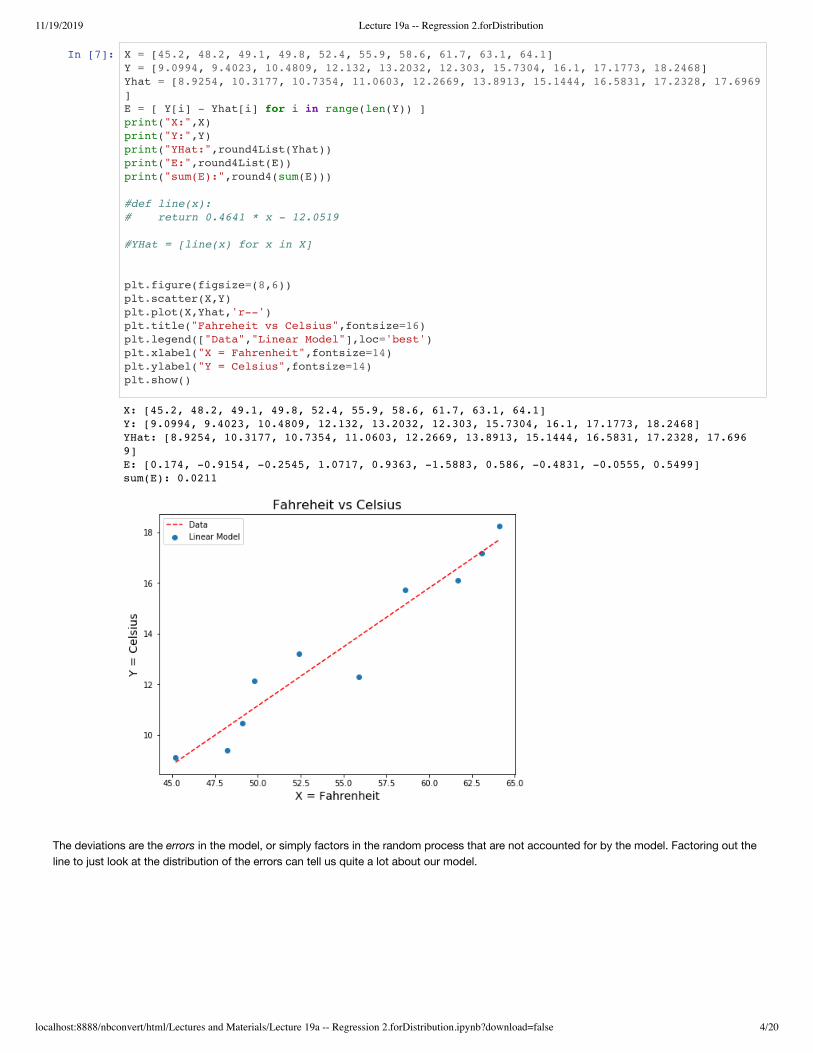
In [8]: X = [45.2, 48.2, 49.1, 49.8, 52.4, 55.9, 58.6, 61.7, 63.1, 64.1] Y = [9.0994, 9.4023, 10.4809, 12.132, 13.2032, 12.303, 15.7304, 16.1, 17.1773, 18.2468]Yhat = [8.9254, 10.3177, 10.7354, 11.0603, 12.2669, 13.8913, 15.1444, 16.5831, 17.2328, 17.6969] plt.figure(figsize=(8,6))plt.title("Regression Line for Data",fontsize=14)plt.xlabel("X = Farenheit Measurements")plt.ylabel("Y = Celsius Measurements")plt.scatter(X,Y)plt.plot(X,Yhat,color='black')plt.scatter(X,Yhat,marker='o',color="black")for k in range(len(X)): plt.plot([X[k],X[k]],[Y[k],Yhat[k]], '--', color='red')plt.show() plt.figure(figsize=(8,6))plt.title("Graph of Residuals",fontsize=14)plt.xlabel("X = Farenheit Measurements")plt.ylabel("Y = Error between Actual and Predicted Values")z = [0 for x in X ]#plt.xlim(-3,4)plt.scatter(X,E)plt.plot(X,z,color='red')plt.ylim(-2,2)plt.show()print("Sum of errors: ",sum(E))



Sum of errors: 0.021100000000000563



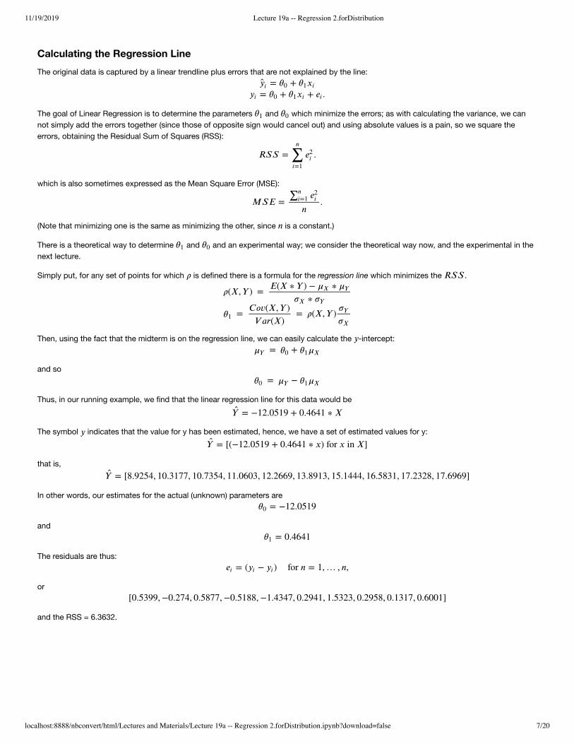
Calculating the Regression LineThe original data is captured by a linear trendline plus errors that are not explained by the line:

The goal of Linear Regression is to determine the parameters and which minimize the errors; as with calculating the variance, we cannot simply add the errors together (since those of opposite sign would cancel out) and using absolute values is a pain, so we square theerrors, obtaining the Residual Sum of Squares (RSS):

which is also sometimes expressed as the Mean Square Error (MSE):

(Note that minimizing one is the same as minimizing the other, since is a constant.)

There is a theoretical way to determine and and an experimental way; we consider the theoretical way now, and the experimental in thenext lecture.

Simply put, for any set of points for which is defined there is a formula for the regression line which minimizes the .

Then, using the fact that the midterm is on the regression line, we can easily calculate the -intercept:

and so

Thus, in our running example, we find that the linear regression line for this data would be

The symbol indicates that the value for y has been estimated, hence, we have a set of estimated values for y:

that is,

In other words, our estimates for the actual (unknown) parameters are

and

The residuals are thus:

or

and the RSS = 6.3632.

= +�̂� 𝑖 𝜃0 𝜃1𝑥𝑖

= + + .𝑦𝑖 𝜃0 𝜃1𝑥𝑖 𝑒𝑖

𝜃1 𝜃0

𝑅𝑆𝑆 = .∑𝑖=1

𝑛

𝑒2𝑖

𝑀𝑆𝐸 = .∑𝑛

𝑖=1 𝑒2𝑖

𝑛

𝑛

𝜃1 𝜃0

𝜌 𝑅𝑆𝑆

𝜌(𝑋, 𝑌 ) =𝐸(𝑋 ∗ 𝑌 ) − ∗𝜇𝑋 𝜇𝑌

∗𝜎𝑋 𝜎𝑌

= = 𝜌(𝑋, 𝑌 )𝜃1

𝐶𝑜𝑣(𝑋, 𝑌 )

𝑉 𝑎𝑟(𝑋)

𝜎𝑌

𝜎𝑋

𝑦

= +𝜇𝑌 𝜃0 𝜃1𝜇𝑋

= −𝜃0 𝜇𝑌 𝜃1𝜇𝑋

= −12.0519 + 0.4641 ∗ 𝑋𝑌 ̂

𝑦

= [(−12.0519 + 0.4641 ∗ 𝑥) for 𝑥 in 𝑋]𝑌 ̂

= [8.9254, 10.3177, 10.7354, 11.0603, 12.2669, 13.8913, 15.1444, 16.5831, 17.2328, 17.6969]𝑌 ̂

= −12.0519𝜃0

= 0.4641𝜃1

= ( − ) for 𝑛 = 1, … , 𝑛,𝑒𝑖 𝑦𝑖 𝑦𝑖

[0.5399, −0.274, 0.5877, −0.5188, −1.4347, 0.2941, 1.5323, 0.2958, 0.1317, 0.6001]



In [9]: # RSS def sumSqDiff(X,Y): s = 0 for k in range(len(X)): s += (X[k] - Y[k])**2 return s muX = mean(X)muY = mean(Y) print("RSS: ", round4(sumSqDiff(Y,Yhat)))print("RSS: ", round4(sumSqDiff(Yhat,[muY]*len(X))))print("TSS: ", round4(sumSqDiff(Y,[muY]*len(X))))

Simple Linear Regression: Building a Linear ModelLinear Regression is the process of constructing a model for a bivariate random variable (X,Y) which shows a linear relationship between X(the independent variable) and Y (the dependent variable). It is assumed that the values taken on by Y are mostly explained by a linearrelationship between X and Y with some variation explained as errors (random deviations from the linear model).

Let us continue with our example of the two thermometers, which gave us a simple way to think about linear regression:

RSS: 6.3632 RSS: 89.9489 TSS: 96.3265



In [10]: print("X:", X)print("Y:",Y)print("Yhat:", Yhat)print("E: ", round4List(E))ScatterTrendline(X,Y,showResiduals=True)

X: [45.2, 48.2, 49.1, 49.8, 52.4, 55.9, 58.6, 61.7, 63.1, 64.1] Y: [9.0994, 9.4023, 10.4809, 12.132, 13.2032, 12.303, 15.7304, 16.1, 17.1773, 18.2468] Yhat: [8.9254, 10.3177, 10.7354, 11.0603, 12.2669, 13.8913, 15.1444, 16.5831, 17.2328, 17.6969] E: [0.174, -0.9154, -0.2545, 1.0717, 0.9363, -1.5883, 0.586, -0.4831, -0.0555, 0.5499]




Definition: Linear Model = "Regression plus errors"When does such a regression line give us an appropriate model of a set of data?The concept of a linear model attempts to answer this question by assuming that the variations from the line are errors which follow a normaldistribution.

A Linear Model for a set of data is a triple , where and are as discussed above, where the set of Residuals is defined as , where

and where that is, where the errors are independent and follow a normal distribution with mean 0 (centered on the line) andstandard deviation

This implies several things about the set of residuals , which are consistent with the view of the residuals as actual errors.

The errors are independent;The mean of the residuals is 0 (which is what you would expect if these really are errors); andThe variance of the errors does not change over the range .

The last criterion has the fancy name "homoscedasticity." and when you don't have it, you have "heteroscedasticity." Here are some simplediagrams showing the idea:

In terms of errors, then heteroscedasticity means the errors get larger as the values get larger, whereas homoscedasticity means the error isindependent of the range of the values.

( , , 𝜎)𝜃0 𝜃1 𝜃0 𝜃1

𝐸 = { , … , }𝑒1 𝑒𝑛

= + +𝑦𝑖 𝜃0 𝜃1𝑥𝑖 𝑒𝑖

𝐸 ∼ 𝑁(0, ),𝜎2

𝜎.

𝐸

𝑋



In [11]: X = [45.2, 48.2, 49.1, 49.8, 52.4, 55.9, 58.6, 61.7, 63.1, 64.1] Y = [9.0994, 9.4023, 10.4809, 12.132, 13.2032, 12.303, 15.7304, 16.1, 17.1773, 18.2468]Yhat = [8.9254, 10.3177, 10.7354, 11.0603, 12.2669, 13.8913, 15.1444, 16.5831, 17.2328, 17.6969]E = [Y[k] - Yhat[k] for k in range(len(X))] import matplotlib.gridspec as gridspec def display2D(x,y,t="Residual Plot",numb=5): fig = plt.figure(figsize=(8,8)) plt.subplots_adjust(wspace=0.3, hspace=0.3) gs = gridspec.GridSpec(2, 2) ax_main = plt.subplot(gs[1:2, :1]) ax_yDist = plt.subplot(gs[1:2, 1],sharey=ax_main) if(len(x) < 20): fmt = 'o' fmt2 = 'o' bord = 3 elif(len(x) <= 100): fmt = '+' fmt2 = '+' bord = 4 else: fmt = ',' fmt2 = '.' bord = 5 ax_main.scatter(x,y,marker=fmt,) #ax_main.set(xlabel="X", ylabel="Y") ax_main.set_title(t,fontsize=12) ax_main.set_ylabel("Y",rotation=0,fontsize=14) ax_main.set_xlabel("X",rotation=0,fontsize=14) ax_main.plot([x[0],x[-1]],[0,0],color="grey") ax_yDist.hist(y,bins=numb,orientation='horizontal',align='mid',edgecolor='black') ax_yDist.set(xlabel='count') ax_yDist.set_title('Y') plt.show() display2D(X,E)



In [12]: ### Another Example def line(x): return 0.4641 * x - 12.0519 X = [45.2, 48.2, 49.1, 49.8, 52.4, 55.9, 58.6, 61.7, 63.1, 64.1] X = [random()*20 + 45 for k in range(100)]Yhat = [line(x) for x in X]E = [normal(0,1) for k in range(len(X))]Y = [Yhat[k] + E[k] for k in range(len(X))] ScatterTrendline(X,Y,showResiduals=True)display2D(X,E)






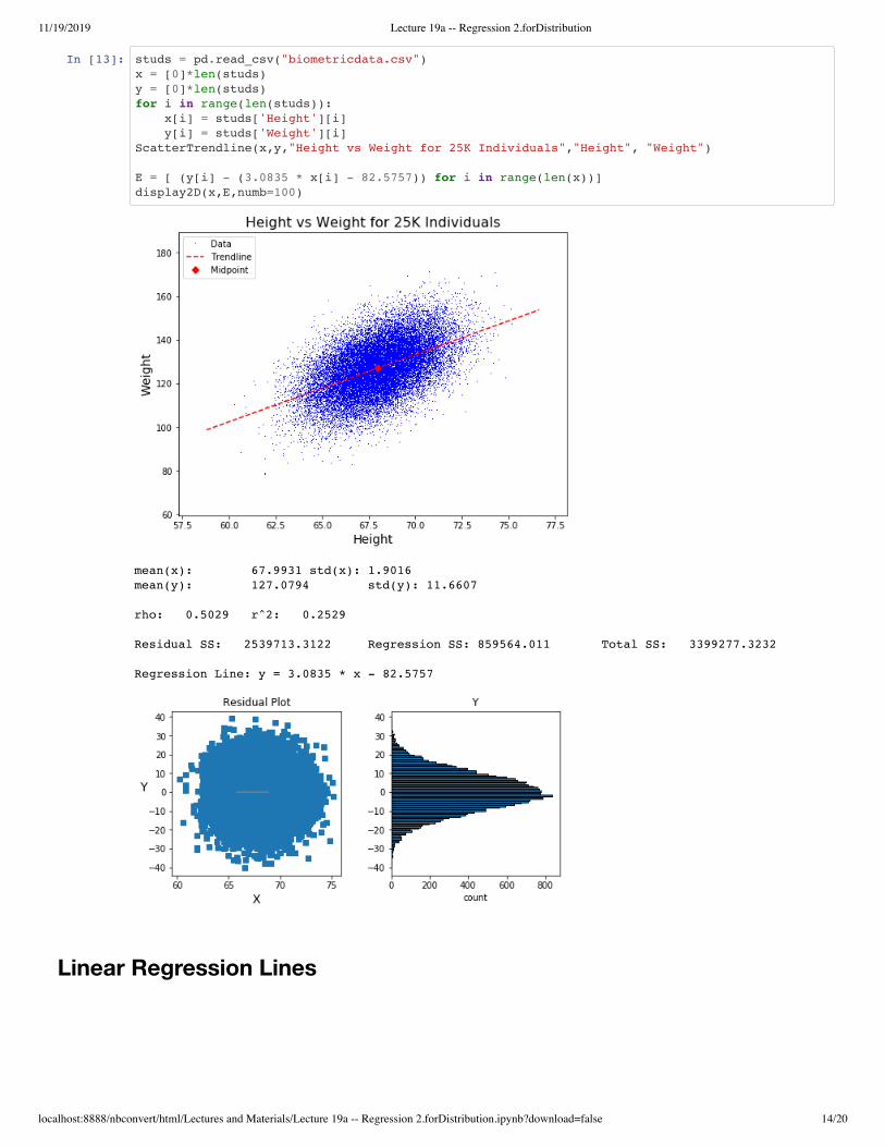
In [13]: studs = pd.read_csv("biometricdata.csv")x = [0]*len(studs)y = [0]*len(studs)for i in range(len(studs)): x[i] = studs['Height'][i] y[i] = studs['Weight'][i]ScatterTrendline(x,y,"Height vs Weight for 25K Individuals","Height", "Weight") E = [ (y[i] - (3.0835 * x[i] - 82.5757)) for i in range(len(x))]display2D(x,E,numb=100)

Linear Regression Lines




In [14]: def Ex0(): x = [1,2,2] y = [1,2,3] ScatterTrendline(x,y,titl="Scatterplot Example 0",xlab="X Data", ylab="Y Data") def Ex1(): x = [5,6,6,7,7,8] y = [6,6,7,8,9,10] ScatterTrendline(x,y,titl="Scatterplot Example 1",xlab="X Data", ylab="Y Data") def Ex2():# x,y = getBioMetricData() x = [50,45,40,38,32,40,55] y = [2.5,5.0,6.2,7.4,8.3,4.7,1.8] ScatterTrendline(x,y,"Scatterplot Example 2","X Data", "Y Data") def Ex3(): studs = pd.read_csv("biometricdata.csv") x = [0]*len(studs) y = [0]*len(studs) for i in range(len(studs)): x[i] = studs['Height'][i] y[i] = studs['Weight'][i] ScatterTrendline(x,y,"Height vs Weight for 25K Individuals","Height", "Weight") def Ex4(): studs = pd.read_csv("StudentData3.csv") x = [0]*len(studs) y = [0]*len(studs) for i in range(len(studs)): x[i] = studs['SAT_TOTAL'][i] y[i] = studs['BU_GPA'][i] ScatterTrendline(x,y,titl="SAT vs GPA", xlab="X = Sat Total",ylab="Y = BU GPA") def Ex5(): studs = pd.read_csv("StudentData3.csv") x = [0]*len(studs) y = [0]*len(studs) for i in range(len(studs)): x[i] = studs['HS_GPA'][i] y[i] = studs['BU_GPA'][i] ScatterTrendline(x,y,titl="HS GPA vs BU GPA", xlab="X = HS GPA",ylab="Y = BU GPA") def midterm(): ScatterTrendline(midtermX,midtermY,titl="CS 237 Midterm Data", xlab="X = MT Score",ylab="Y = Time Turned In") X = [45.2, 47.1, 47.5, 49.6, 49.8, 52.0, 54.3, 58.6, 63.2, 64.1] Y = [7.8752, 8.117, 9.2009, 9.3167, 8.4564, 11.4075, 13.9236, 15.0762, 17.4678, 18.4362] ScatterTrendline(X,Y,"Fahrenheit vs Celsius",xlab="X = Farenheit",ylab="Celsius") print("\n\nExample 0") Ex0() print("\n\nExample 1") Ex1()print("\n\nExample 2")Ex2()print("\n\nExample 3")Ex3()print("\n\nExample 4")Ex4()print("\n\nExample 5")Ex5()print("\n\nMidterm Data")midterm()





mean(x): 53.14 std(x): 6.3938 mean(y): 11.9278 std(y): 3.8009 rho: 0.9817 r^2: 0.9638 Residual SS: 5.2364 Regression SS: 139.231 Total SS: 144.4674 Regression Line: y = 0.5836 * x - 19.0844 Example 0





mean(x): 42.8571 std(x): 7.1799 mean(y): 5.1286 std(y): 2.2218 rho: -0.9562 r^2: 0.9143 Residual SS: 2.9625 Regression SS: 31.5918 Total SS: 34.5543 Regression Line: y = -0.2959 * x + 17.8093 Example 3




mean(x): 1282.4211 std(x): 112.7056 mean(y): 2.9943 std(y): 0.6129 rho: 0.269 r^2: 0.0724 Residual SS: 33.1077 Regression SS: 2.583 Total SS: 35.6907 Regression Line: y = 0.0015 * x + 1.1181 Example 5



mean(x): 3.4968 std(x): 0.4035 mean(y): 2.9943 std(y): 0.6129 rho: 0.4015 r^2: 0.1612 Residual SS: 29.9369 Regression SS: 5.7538 Total SS: 35.6907 Regression Line: y = 0.6099 * x + 0.8617 Midterm Data

mean(x): 12.6125 std(x): 4.4229 mean(y): 71.1375 std(y): 16.4474 rho: -0.036 r^2: 0.0013 Residual SS: 21613.3788 Regression SS: 28.1087 Total SS: 21641.4875 Regression Line: y = -0.134 * x + 72.8278

Documents

Correlation and Materials/Lect… · The correlation coeﬃcient is so the experimental data show a strong linear correlation. It seems that we should be able to ﬁnd a line that