Embed Size (px)
Citation preview

arX
iv:c
ond-
mat
/970
1185
v2 2
8 Ja
n 19
97
Second Virial Coefficient For Real Gases
At High Temperature∗
H. Boschi-Filho†‡ and C.C.Buthers‡† Center for Theoretical Physics, Laboratory for Nuclear Science
Massachusetts Institute of Technology
Cambridge, Massachusetts 02139-4307, USAand
‡Instituto de Fısica, Universidade Federal do Rio de JaneiroCidade Universitaria, Ilha do Fundao, Caixa Postal 68528
21945-970 Rio de Janeiro, BRAZIL
January 24, 1997
Abstract
We study the second virial coefficient, B(T ), for simple real gases at high tem-perature. Theoretical arguments imply that there exists a certain temperature, Ti,for each gas, for which this coefficient is a maximum. However, the experimentaldata clearly exhibits this maximum only for the Helium gas. We argue that this is sobecause few experimental data are known in the region where these maxima shouldappear for other gases. We make different assumptions to estimate Ti. First, weadopt an empirical formulae for B(T ). Secondly, we assume that the intermolecularpotential is the Lennard-Jones one and later we interpolate the known experimentaldata of B(T ) for Ar, He, Kr, H2, N2, O2, Ne and Xe with simple polynomials ofarbitrary powers, combined or not with exponentials. With this assumptions weestimate the values of Ti for these gases and compare them.
PACS: 34.20.-b; 05.70.Ce; 65.50.+m; 33.15.-e.
∗This work is supported in part by funds provided by the U.S. Department of Energy (D.O.E.)under cooperative research agreement #DF-FC02-94ER40818 and Conselho Nacional de DesenvolvimentoCientıfico e Tecnologico (CNPq) - Brazilian agency.
†E-mail address: [email protected]
1

1 Introduction
Long time ago, Kamerlingh Onnes and collaborators performed a systematical study of
physical properties of gases at low temperature, measuring their deviations from the ideal
gas law, or in other words, determining their virial coefficients [1]-[3]. Since then, much
research has been done in this direction collecting more and more data for many different
substances, mainly at low temperature [4]. In particular, in 1925, Holborn and Otto
studied some simple gases (Ar, He, H2, N2, and Ne) and they were able to determine an
empirical formula for the second virial coefficient, B(T ), which constituted at that time
and persists until today as a land-mark work in physics [5].
On the other hand and at the same time, Lennard-Jones showed in another remarkable
work that for intermolecular potentials written as binomials of arbitrary powers of the
intermolecular distance, the corresponding second virial coefficient B(T ) can be calculated
exactly as an infinite power series [6]. This kind of potential describes very well the
behavior of simple molecules as the one studied by Kamerlingh Onnes, Holborn and
Otto and others. Also, other types of intermolecular potentials have been discussed
but without exact integrability [7]. Despite of the long time that these empirical and
theoretical expressions for B(T ) are known, they are usually not equal. This can be
understood paying attention to the fact that the experimental data available for most
substances are restricted to a certain range of temperatures, usually below 600K. The
choice for low temperature physics seems rather natural if one, for example, is looking for
critical phenomena in condensed matter which can be almost entirely found in this region.
However, the high temperature behavior of real gases can also be of interest, for example,
in the study of hot plasma and in many situations in astrophysics as nucleosynthesis,
super-novae, etc.
Here in this paper, we are going to examine the second virial coefficient of some real
simple gases (Ar, He, Kr, H2, N2, O2, Ne and Xe) at high temperature. This is not an
easy task since few data for these and other gases are available for temperatures above
the range 600 ∼ 1000K. The main point of this work is that we can show from measures
2
of B(T ) that most of these real simple gases admits a maximum value corresponding to
a certain temperature for each gas, which may be called an inversion temperature (Ti).
The existence of this maximum may be not a surprise once it is already present, for the
Helium, in Holborn and Otto work [5]. However, for all other real gases they are not yet
known. Anyway, some previous discussions on this maximum [8] and on this inversion
temperature [9] can be found in the literature.
This paper is organized as follows: in section 2, we discuss the inversion temperature
Ti associated with the Joule or free expansion and recall the well known inversion temper-
ature related to the Joule-Thomson throttling process, TiJT . We show that there is a kind
of duality between the equations governing these two temperatures. The temperatures
TiJT are known experimentally and can also be obtained by various theoretical methods,
one of them assumes the knowledge of an equation of state. We show, however, that the
known equations of state do not lead to any finite Ti. In section 3, we employ different
methods to estimate the inversion temperature Ti. The first and simplest one is to use
the empirical expression for B(T ) given by Holborn and Otto from which we can find
easily its maximum. The second and third methods are based on the assumption that
the intermolecular potential between the molecules of the real gas is the Lennard-Jones
6-12 potential [6]. So, the second method consists in finding the inversion temperature Ti
evaluating dB/dT = 0 numerically. The third method is a variation of the second since
the assumption of the Lennard-Jones potential permit us to relate the temperatures Ti
and TiJT , determining the former, once the latter are well known. The fourth and last
method for determining Ti, that we discuss in this paper, is a numerical analysis of the
experimental data for B(T ) for the above mentioned gases. We interpolate these data
with simple polynomial functions with arbitrary powers with and without exponentials
terms. In section 4, we compare the results obtained from these functions with the ones
from other methods and present our conclusions.
3

2 The Inversion Temperatures Ti and TiJT
The inversion temperature Ti, for which B(T ) is a maximum, has a simple physical
interpretation. A real gas, initially at this temperature, subjected to a free expansion
remains at this temperature for any change in its volume, which is the ideal gas behavior,
for any initial temperature. If the real gas initial temperature is greater than Ti then it
will get hotter in a free expansion and the reverse occurs if T < Ti, which is our ”daily”
experience. One can understand this simply by noting that the Joule coefficient, i.e., the
variation of temperature against volume in a free expansion (with internal energy U being
constant) can be expressed as [10]
J ≡ (∂T
∂V)U
=1
cV
[P − T (∂P
∂T)V ]. (2.1)
Writing the virial expansion as
PV = RT (1 +B
V+
C
V 2+
D
V 3+
E
V 4+ ...) (2.2)
it is easy to show that, in the thermodynamical limit (V → ∞)
J = − RT 2
cV V 2(dB
dT), (2.3)
where B ≡ B(T ). Looking at the above expression one can see that the maximum of
B(T ), which may occur for certain values of T = Ti, vanishes the Joule coefficient J :
J = 0 ⇔ dB
dT= 0. (2.4)
Assuming that Ti is unique, above this temperature J will be positive and so the temper-
ature increases under a free expansion. Bellow Ti the temperature decreases.
In fact, this behavior is also expected in the bases of the Yang and Lee Theorem [11]
(see also [8]) if one assumes that the intermolecular potential of the gas has a shape as
the one given by fig.1. This is a typical shape which includes the well known Lennard-
Jones, Stockmayer and other potentials [7]. This kind of potential implies a maximum for
4
B(T ) since they are not infinite for finite distances between molecules, contrary to what
happens for the hard-sphere case, for example.
At this point, it is interesting to discuss a well known inversion temperature, TiJT , that
one associated with the Joule-Thomson throttling process with constant enthalpy and its
relation to the previous discussed inversion temperature Ti. The relevant coefficient in
this case can be written as [10]
µ =1
cP
[T (∂V
∂T)P − V ]. (2.5)
As the derivative of the volume in respect to the temperature must be calculated under
constant pressure, the virial expansion (2.2) is not the most appropriate in this case and
it is usual to rewrite it as
PV = RT (1 + BPP + CPP 2 + DPP 3 + EP P 4 + ...), (2.6)
so we get immediately, in the low pressure limit (P → 0)
µ =RT 2
cP
(dBP
dT). (2.7)
The inversion temperature, in this process, TiJT , is determined by the vanishing µ:
µ = 0 ⇔ dBP
dT|T=TiJT
= 0. (2.8)
These temperatures, apart from being well known for most real gases, are of great practical
importance, for example, to improve the efficiency of thermal engines as refrigerators [12].
Another striking property of this temperature is its resemblance with Ti. This is not a
coincidence since the second virial coefficients at constant volume and pressure, B and
BP , respectively, are simply related by
B = BPRT. (2.9)
So, we can trace a parallel between these two inversion temperatures first substituting
the above expression into eq.(2.7) so we get
µ = 0 ⇔ dB
dT=
B
T; T = TiJT , (2.10)
5

which is the usual expression for the throttling process [7] and then into eq. (2.3)
J = 0 ⇔ dBP
dT= −BP
T; T = Ti, (2.11)
for the Joule expansion. Comparing eqs. (2.4) and (2.8), (2.10) and (2.11) one can see
clearly a kind of duality between the equations governing these two processes: The role
played by the inversion temperature TiJT in the constant enthalpy process is analogous
to the Ti in the constant energy case. Despite of this appealing resemblance the inversion
temperature Ti for the Joule process has been rarely discussed [9], and these discussions
are for from being satisfactory or complete.
The temperatures TiJT are known experimentally and can also be estimated using
simple equations of state [10]. One can wonder if the inversion temperature Ti can be
found from equations of state as happens for TiJT . This should be nice, but for various
equations of state the corresponding second virial coefficient does not allow any finite Ti, as
can be seen by inspection of Table 1. Note that B(T ) for the Beattie-Bridgeman equation
of state admits in principle a maximum, but actually as the values of the constants a and
c are positive for real gases one finds that no real Ti are admissible from this equation
too.
3 Estimates On The Inversion Temperature Ti
There are various possible ways of computing Ti. We will discuss some of them and
compare their results. If one knows the correct expression for B(T ) then the problem
would be trivial, since the equation dB/dT = 0 could be solved immediately. But what
we have until now are, on one side expressions for B(T ) based on theoretical assumptions
and on the other side empirical expressions which differ in general from each other and
are constructed on the data for which the temperatures are low, usually under 600K. As
we are going to show, these maxima appear in a region beyond this temperature, except
for the Helium, for which Ti ≃ 200K [5].
6

Among the known expressions for B(T ), the most simple is, perhaps, the Holborn and
Otto [5] one
B(T ) = a + bT +c
T+
e
T 3, (3.1)
from which one can easily find that the inversion temperature, in this case is given by
Ti =
√
c −√
c2 + 12eb
2b. (3.2)
The values of the coefficients appearing in eq. (3.1) and the corresponding Ti’s for some
simple gases are found in Table 2.
From statistical mechanics, it is well known that an intermolecular potential, u(~r),
and the corresponding the second virial coefficient are related by:
B(T ) =1
2
∫
Vd~r [1 − exp(−u(~r)/kT )], (3.3)
where k is the Boltzmann constant. So, the inversion temperature Ti could also, in
principle, be obtained analytically through this expression. However, this is a formidable
task for almost of known intermolecular potentials except from the trivial ones like the
hard-sphere, which does not imply any finite Ti. An important exception is the Lennard-
Jones potential [6]:
uLJ(r) = ǫ0[(r0
r)12 − 2(
r0
r)6], (3.4)
for which B(T ) can be computed exactly as an infinite power series. The constants ǫ0 and
r0 are tabulated for many real gases. Substituting (3.4) into (3.3) one can show that [7]
B(T ) = b0
∞∑
j=0
b(j)T ∗−
(2j+1)4 , (3.5)
where T ∗ = kTǫ0
is the reduced temperature, b0 =√
23
πnr30, n being the number of molecules
per mol and
b(j) = −2j+ 12
4j!Γ(
2j − 1
4). (3.6)
7

The importance of this potential is related to the fact that it describes the Van der Walls
force of attraction between molecules, which is proportional to r−7(in the non-relativistic
limit) and includes a finite repulsion at small finites distances, being integrable and fitting
(low temperature) data quite well for a great number of real gases. For this potential, we
can evaluate the inversion temperature Ti, since
dB(T )
dT= −ǫ0b0
kT ∗
∞∑
j=0
(2j + 1)
4b(j)T ∗
−
(2j+1)4 (3.7)
and imposing thatdB(T )
dT= 0, (3.8)
which solution can be evaluated numerically. As the expected inversion temperature is of
order 102 ∼ 103K, we see that the series in eq.(3.7) is rapidly convergent. Taking j = 5
we find
T ∗i =
kTi
ǫ0
∼= 25.152 (3.9)
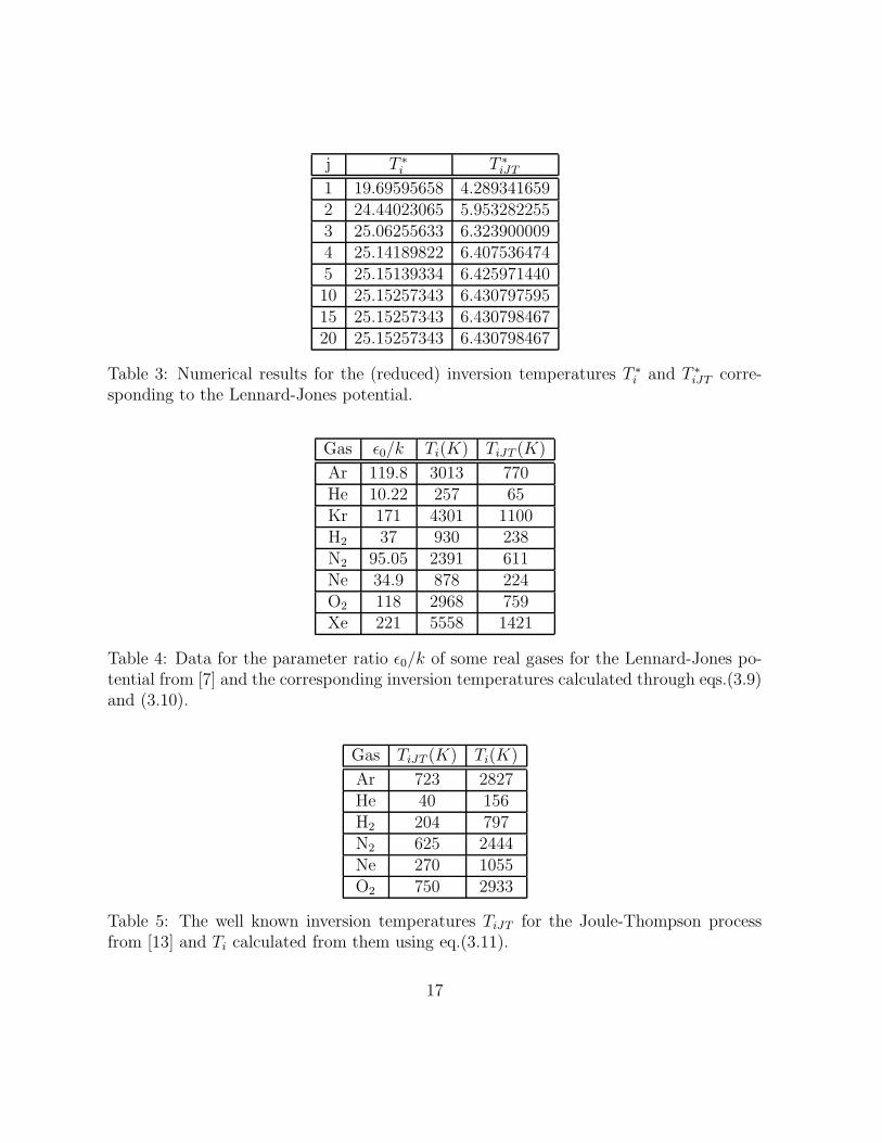
with precision of 0.001. If we extend this calculation until j = 15, for example, it will
change less than 0.001 (see Table 3). Using the data for ǫ0 from [7] in the above equation,
we can estimate the inversion temperature for mono-atomic and diatomic (and perhaps
for simple poly-atomic gases) which results can be seen in Table 4.
A related analysis can also be made for the inversion temperature TiJT of the throttling
process. Starting from the expression for B(T ), eq. (3.5), corresponding to the Lennard-
Jones potential and imposing the conditions (2.10) we find (see Table 3)
T ∗iJT =
k
ǫ0
TiJT∼= 6.431 (3.10)
As these temperatures are well known, comparing eqs.(3.9) and (3.10) we can also find
Ti from them:
Ti ≃ 3.911 TiJT , (3.11)
when we assume that the intermolecular potential is the Lennard-Jones one. The temper-
atures calculated using this relation are shown in Table 5. These numerical results could
8

also be inferred from tabulated values of B(T ) and its derivatives for the Lennard-Jones
potential [7] (see also [9]).
As our last method for computing Ti, we will consider polynomial expressions for
B(T ), combined or not with exponential terms, which parameters will be fixed by best
fitting of experimental data from [4]. The first and simplest case is
B1(T ) =a
T b+
c
T d(3.12)
and we will use Powell’s method from Numerical Recipes [14] to minimize χ2, defined by
χ2 =N
∑
n=1
[BL(Tn) − Bexp(Tn)]2 (3.13)
where BL(Tn), with L = 1, is the expression (3.12) calculated with N experimental
temperature values Tn, (n = 1, ..., N) and Bexp(Tn) are the corresponding experimental
values for the second virial coefficient. In Table 6, we give the coefficients of (3.12) which
minimize χ2 for each gas and present the inversion temperature Ti calculated from them.
In fact, except for the Helium, these values of Ti correspond to extrapolations on the
interpolated expressions of B1(T ).
In order to improve these results we also consider other functions for B(T ), which are
B2(T ) =a
T b+
c
T d+
e
T f(3.14)
B3(T ) =a
T b+
c
T d+ f exp(−gT ) (3.15)
B4(T ) =a
T b+
c
T d+
e
T f+ g exp(−hT ). (3.16)
and repeat the above procedure, as was done for B1(T ). The corresponding results for
B2(T ), B3(T ) and B4(T ) are shown in Tables 7, 8 and 9, respectively. The data we have
used for B(T ) for these gases are the ones which were compiled by Dymond and Smith
[4]. In particular, for the Argon we used N = 36 experimental data from [5], [15], [16] and
[17]. For the Helium we used N = 31 experimental data from [5],[18], [19] and [20]. For
the Krypton we used N = 28 experimental data from [21], [22] and [23]. For the Hydrogen
9

we used N = 30 experimental data from [1], [5], [15] and [24]. For the Nitrogen we used
N = 38 experimental data from [3], [5], [19] and [25]. For the Neon we used N = 19
experimental data from [5] and [26]. For the Oxygen we used N = 20 experimental data
from [2], [5], [27] and [28]. Finally, for the Xenon we used N = 30 experimental data from
[29], [30] and [31].
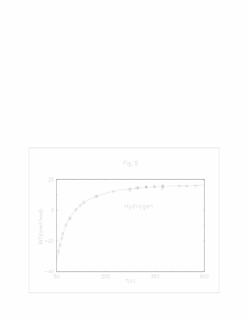
To get more confidence on these results, we have also shown them graphically in figures
2 to 9. In these figures we have plotted the best fitting for eqs. (3.12) and (3.14) - (3.16),
for each gas separately. Note that for the most of gases only one curve can be seen since
the fittings are very close to each other. In particular, in fig. 3 (Helium) three different
curves can be seen, corresponding to the equations (3.12) and (3.14) - (3.16). In this case
the fitting represented by eqs. (3.15) and (3.16) are very close to each other.
4 Discussion and Conclusions
We have estimated the inversion temperature Ti related to the Joule or free expansion
by different methods. As can be seen from tables 2 and 4 to 9, each gas has a different
inversion temperature Ti, which depend also on the method employed. In some cases as
for the Hydrogen the values found can differ by a factor of 2 and for the Nitrogen by 4.
Another gases as the Helium and Argon the discrepancy was about a factor of 5/3 and
3/2, respectively. Taking this into account and using a χ2-weighted average, we estimate
a value for Ti corresponding to each gas, basically from the numerical fitting expressed
in Tables 6 – 9, which results can be seen in Table 10. The choice for taking only the
temperatures from Tables 6 – 9 is based on the fact that the values from these tables are
the ones in which minimum modeling assumptions were made, since we left the powers
of the polynomials (3.12) and (3.14) - (3.16) to be fixed by best fitting to experimental
data, contrary to what happens in the other methods that we discussed before. Looking
at Table 10 one can also see that for the Oxygen and Krypton we could not find values
for Ti, despite that from Tables 4 and 5 we can see, by other methods some values for
them.
10

To give an idea of the global behavior of the expressions for B(T ) and to visualize
some of the maxima corresponding to the inversion temperature Ti discussed above, we
have plotted in a single graph (see fig. 10) the shape of eq. (3.16) which we found for
all the gases discussed in this paper until temperatures of the order of 4 × 10³K. As one
can see from this graph some gases as the Helium, of course, and the Hydrogen exhibits
clearly these maxima. For some others as the Neon, Argon and Nitrogen these maxima
can be seen in a careful analysis, while for the Krypton, Xenon and Oxygen they can not
be seen in this range of temperatures.
To conclude, we can say that the inversion temperature Ti associated with the free
expansion of a real gas can be determined for some simple gases and in general they
were not known because there are few experimental data for the range of temperatures
in which they should appear. Despite that the physical interpretation of the inversion
temperature Ti is related to a free expansion which is a non-equilibrium process and so
difficult to analyze directly, the values for B(T ) can be taken from usual PV T measures.
An important consequence of determining precisely this inversion temperature is that it
will permit a greater confidence between the experimental and theoretical expressions for
B(T ) and consequently on the force between molecules.
Acknowledgments: We would like to acknowledge F.M.L. de Almeida, A.S. de Castro
and Y.A. Coutinho for the help with different computational parts of this work and
specially A. Ramalho who wrote a Fortran program which enable us to use the Powell
routine of Numerical Recipes. H.B.-F. acknowlegdes R. Jackiw for his hospitality at MIT
and for reading the manuscript and K. Huang for an interesting discussion on these
results. The authors were partially supported by CNPq – Brazilian agency (C.C.B. under
the CNPq/PIBIC program).
11

References
[1] H.Kamerlingh Onnes and C.Braak, Communs Phys. Lab. Univ. Leiden, 100b,(1907).
[2] H. A. Kuypers and H. Kamerlingh Onnes, Archs neerl. Sci., 6,277,(1923).
[3] H. Kamerlingh Onnes and A. T. van Urk, Communs Phys. Lab. Univ. Leiden, 169d,
e,(1924).
[4] A compilation of the virial coefficients for many different substances can be found in:
J. H. Dymond and E. B. Smith,The Virial coefficients of Pure Gases and Mixtures.
Oxford, Clarendon, (1980).
[5] L. Holborn and J. Otto, Z. Physik 33,1,(1925).
[6] J. E. Lennard-Jones, Proc. Roy. Soc. , London, A106, 463, (1924).
[7] For a review see: J. O. Hirschfelder, C. F. Curtiss and R. B. Bird, Molecular theory
of gases and Liquids. New York, Wiley, (1954).
[8] S. K. Ma, Statistical Mechanics. Singapore, World Scientific, (1985).
[9] B. Roulet and J-O. Goussard, Am. J. Phys. 61, 845, (1993).
[10] See e. g. G. W.Castellan, Physical Chemistry, 2nd. ed. Reading, Addison-Wesley,
(1971).
[11] C. N. Yang and T. D. Lee, Phys. Rev., 87, 404, (1952).
[12] See e. g. F. C. Andrews, Thermodynamics: Principles and Applications, New York,
Wiley, (1971).
[13] A. Kestin, Course in Statistical Thermodynamics. New York, Academic, (1971).
[14] W.H. Press, S.A. Teukolsky, W.T. Vetterling and B.P. Flannery, Numerical Recipes
in Fortran, 2nd ed. Cambridge Univ. Press, 1992.
12

[15] C. C. Tanner and I. Masson, Proc. R. Soc., A126, 268, (1930).
[16] E. Whalley, Y. Lupien and W. G. Schneider, Can. J. Chem., 31,722,(1953).
[17] B. E. F. Fender and G. D. Halsey,Jr., J. Chem. Phys.,36,1881,(1962).
[18] D. White, T. Rubin, P. Camky and H. L. Johnston, J. Phys. Chem., Ithaca
64,1607,(1960).
[19] R. J. Witonsky and J. G. Miller, J. Am. Chem. Soc., 85,282,(1963).
[20] N.K. Kalfoglou and J.G. Miller, J. Phys. Chem., Ithaca 71,1256,(1967).
[21] J. A. Beattie, J. S. Brierley and R. J. Barriaut, J. Chem. Phys.,20,1615,(1952).
[22] E. Whalley and W. G. Schneider, Trans. Am. Soc. Mech. Engng., 76,1001,(1954).
[23] H. P.Rentschler and B.Schramm, Ber.(dtsch) Bunsenges. Phys. Chem.,81,319,(1977).
[24] C. W. Gibby, C. C. Tanner and I. Masson, Proc. R. Soc., A122,283,(1928).
[25] J. A. Huff and T. M. Reed, J. Chem. Engng Data 8,306,(1963).
[26] G. A. Nicholson and W. G. Schneider, Can. J. Chem., 33,589,(1955).
[27] A. Michels, H. W. Schamp and W. de Graaff, Physica, ’s Grav. 20,1209,(1954).
[28] G. P. Nijhoff and W. H. Keesom, Communs phys. Lab. Univ. Leiden, 179b,(1925).
[29] J.A. Beattie, R. J. Barriault and J. S. Brierley, J. Chem. Phys., 19,1222,(1951).
[30] A. Michels, T. Wassenaar and P. Louwerse, Physica, ’s Grav. 20,99,(1954).
[31] E. Whalley, Y. Lupien and W. G. Schneider, Can. J. Chem., 33,633,(1955).
13

Figure Captions
Fig. 1: A typical shape for intermolecular potential as the one given by the Lennard-
Jones potential.
Fig. 2: The second virial coefficient, B(T ), for the Argon. The curve represents eqs.(3.12)
and (3.14) - (3.16) best fitting experimental data from: © – Holborn and Otto [5]; ⊔⊓ –
Tanner and Masson [15]; △ – Walley, Lupien and Schneider [16]; ▽ – Fender and Halsey
[17].
Fig. 3: The second virial coefficient, B(T ), for the Helium. The curves represent
eqs.(3.12) and (3.14) - (3.16) best fitting experimental data from: ⊔⊓ – Holborn and Otto
[5]; © – White, Rubin, Camky and Johnston [18]; △ – Witonsky and Miller [19]; ▽ –
Kalfoglou and Miller [20]. Note that eqs. (refb3) and (3.16) can not be distinguisehd in
this graph.
Fig. 4: The second virial coefficient, B(T ), for the Krypton. The curve represents
eqs.(3.12) and (3.14) - (3.16) best fitting experimental data from: © – Beattie, Brierley
and Barriaut [21]; ⊔⊓ – Walley and Schneider [22]; △ – Rentschler and Schramm [23].
Fig. 5: The second virial coefficient, B(T ), for the Hydrogen. The curve represents
eqs.(3.12) and (3.14) - (3.16) best fitting experimental data from: ⊔⊓ – Kamerlingh Onnes
and Braak [1]; © – Holborn and Otto [5]; △ – Tanner and Masson [15]: ▽ – Gibby,
Tanner and Masson [24].
Fig. 6: The second virial coefficient, B(T ), for the Nitrogen. The curve represents
eqs.(3.12) and (3.14) - (3.16) best fitting experimental data from: ⊔⊓ – Kamerlingh Onnes
and Van Urk [3]; © – Holborn and Otto [5]; ▽ – Witonsky and Miller [19]; △ – Huff and
Reed [25].
14

Fig. 7: The second virial coefficient, B(T ), for the Neon. The curve represents eqs.(3.12)
and (3.14) - (3.16) best fitting experimental data from: ⊔⊓ – Holborn and Otto [5]; © –
Nicholson and Schneider [26].
Fig. 8: The second virial coefficient, B(T ), for the Oxygen. The curve represents
eqs.(3.12) and (3.14) - (3.16) best fitting experimental data from: ⊔⊓ – Kuypers and H.
Kamerlingh Onnes [2]; © – Holborn and Otto [5]; ▽ – Michels, Schamp and Graaff [27];
△ – Nijhoff and W.H. Keesom [28].
Fig. 9: The second virial coefficient, B(T ), for the Xenon. The curve represents eqs.(3.12)
and (3.14) - (3.16) best fitting experimental data from: ⊔⊓ – Beattie, Barriault and Brierley
[29]; © – Michels, Wassenaar and Louwerse [30]; △ – Walley, Lupien and Schneider [31].
Fig. 10: An overview of the second virial coefficients represented by eq.(3.16) as the
best fit for the gases discussed in this paper. We extrapolated these functions to high
temperatures in order to search for their maxima. As one can see, some of them clearly
exhibits a maximum, as the case of Helium and Hydrogen; for Neon, Argon and Nitrogen
they appear slightly and for the others we can not see them, at least for this range of
temperatures.
15

Author Equation B(T ) Ti
Van der Waals PV = RT + bP − aV
+ abV 2 b − a
RT∞
Berthelot PV = RT + bP − aTV
+ abTV 2 b − a
RT 2 ∞
Dieterici PV = RTexp(− aRTV
) + bP b − aRT
∞
Redlich-Kwong PV = RT + bP − a√T
b –
Beattie-Bridgeman PV = RT + DV
+ EV 2 + F
V 3 b − aRT
− cT 3
√
−3cRa
Table 1: Equations of state and respectives B(T); a, b and c are different constants foreach equation and gas while D, E and F are functions of T [10]. From these B(T )and solving dB/dT = 0 one finds Ti. The only possible choice for finite Ti among theseequations is the Beattie-Bridgeman equation of state. However, as a and c in this equationare positive constants for all real gases, we can see that none of the above equations leadto any real finite Ti.
Gas a x 105 b x 107 c x 103 e x 10−1 Ti(K)
Ar 251.00 -2.40 -972.00 -345.60 2015He 87.01 -3.31 -18.77 – 222H2 166.00 -7.66 -172.33 – 474N2 357.46 -9.36 -1044.84 -242.53 1123Ne 102.10 -0.80 -100.00 -31.33 1259
Table 2: Coefficients of the eq.(3.1) for B(T ) from Holborn and Otto [5] and Ti calculatedfrom eq.(3.2).
16
j T ∗i T ∗
iJT
1 19.69595658 4.2893416592 24.44023065 5.9532822553 25.06255633 6.3239000094 25.14189822 6.4075364745 25.15139334 6.42597144010 25.15257343 6.43079759515 25.15257343 6.43079846720 25.15257343 6.430798467
Table 3: Numerical results for the (reduced) inversion temperatures T ∗i and T ∗
iJT corre-sponding to the Lennard-Jones potential.
Gas ǫ0/k Ti(K) TiJT (K)
Ar 119.8 3013 770He 10.22 257 65Kr 171 4301 1100H2 37 930 238N2 95.05 2391 611Ne 34.9 878 224O2 118 2968 759Xe 221 5558 1421
Table 4: Data for the parameter ratio ǫ0/k of some real gases for the Lennard-Jones po-tential from [7] and the corresponding inversion temperatures calculated through eqs.(3.9)and (3.10).
Gas TiJT (K) Ti(K)
Ar 723 2827He 40 156H2 204 797N2 625 2444Ne 270 1055O2 750 2933
Table 5: The well known inversion temperatures TiJT for the Joule-Thompson processfrom [13] and Ti calculated from them using eq.(3.11).
17

Gas a x 105 b c d χ2 Ti(K)
Ar -3.8458 1.6470 1.4676 -0.42510 39.84 -He -0.00037874 0.19433 -731.41 1.1205 7.80 162Kr 12.884 1.7316 0.2639 -0.68291 7.36 -H2 0.053319 1.1250 62.656 0.1747 4.77 762N2 -1.7851 1.4891 -0.075169 21.124 8.072 -Ne 0.0009038 0.24146 -3873.2 1.0229 0.99 -O2 -12.758 1.9062 7.3866(-4) -1.6421 3.20 -Xe -5.8075 1.4302 20.145 -0.11510 54.04 -
Table 6: Coefficients of eq.(3.12) fitting experimental data compiled in [4] and the corre-sponding Ti. See captions of figs. 2 – 9 for details concerning experimental data used inthe numerical treatment for each gas.
Gas a b c d e f χ2 Ti(K)
Ar -1.3342(5) 1.4215 -3.2404(8) 3.6778 11.018 -0.14186 33.10 -He -3244.5 1.8348 5.5676 -0.29099 -0.79394 -0.54227 3.81 225Kr 6.9839(49) 20.404 3.0730(6) 1.8976 0.062216 -0.88609 6.78 -H2 -10127 1.0608 5074.5 1.0204 65.673 0.18220 4.76 742N2 -27.083 1.0338 -3.0304(10) 4.4904 368.82 0.29037 6.59 1779Ne -3203.8 0.85450 4.8903(-4) -1.1751 426.34 0.43549 0.91 -O2 7.7283(-4) -1.6345 -1.2825(6) 1.9066 25352 2.2728 3.20 -Xe 8.2799(5) 1.2173 -1.3374(6) 1.2710 2.9953 -0.36180 53.67 -
Table 7: Coefficients of eq.(3.14) fitting experimental data compiled in [4] and the cor-responding Ti. The number between parenthesis represents the decimal power of eachcoefficient. See captions of figs. 2 – 9 for details concerning experimental data used inthe numerical treatment for each gas.
18

Gas a b c d f g χ2 Ti(K)
Ar -1.7016 1.4586 -6.6200(15) 7.6571 24.387 -1.8960 28.21 -He -608.29 1.1845 -2.1380(14) 11.665 14.480 5.2356 2.14 199Kr -1.0322(7) 2.0942 1.5424(16) 6.2812 7.7358 -13.232 6.64 -H2 -1.7658(5) 1.2639 1.6979(5) 1.2655 22.693 3.1394 4.58 574N2 42.198 0.050811 -1.5131(6) 2.0026 -73.672 44.518 6.32 -Ne -7354.0 1.2176 43.256 0.14858 2017.9 1142.3 0.90 873O2 -6.6122(5) 1.7889 -1.5766(6) 2.3994 3.5171 -37.111 3.07 -Xe -5.6145(6) 1.7824 1.7444(8) 2.6786 23.081 4.5891 52.82 1870
Table 8: Coefficients of eq.(3.15) fitting experimental data compiled in [4] and the cor-responding Ti. The number between parenthesis represents the decimal power of eachcoefficient. See captions of figs. 2 – 9 for details concerning experimental data used inthe numerical treatment for each gas.
Gas a b c d e f g h χ2 Ti(K)
Ar -40619 1.0683 -3.7726(15) 7.4168 154.41 0.17160 77.936 48.300 26.47 3841He -4.5828(-3) -0.50182 -606.47 1.1823 -6.6369(15) 12.931 14.540 5.1296 2.12 199Kr -1.8199(6) 1.8400 -3.3257(8) 2.8883 1.0915(13) 4.8686 9.1254 -11.701 6.58 -H2 -123.49 1.1909 5960.4 1.1763 19.971 0.86958 23.248 3.5224 4.58 549N2 -14734 0.95513 -3.1691(7) 2.8771 155.79 0.16280 -9.3920(-3) -69.007 6.24 3130Ne -12337 1.3439 2.4123 -0.053448 34.092 0.15637 -128.42 565.23 0.88 -O2 4.9441(-7) -2.8490 -3.5770(6) 2.1115 3.2702(14) 6.5228 -0.025554 -85.016 1.90 -Xe -1.8835(5) 1.0629 2.4642(7) 2.3383 239.78 0.10465 326.00 28.401 52.25 -
Table 9: Coefficients of eq.(3.16) fitting experimental data compiled in [4] and the cor-responding Ti. The number between parenthesis represents the decimal power of eachcoefficient. See captions of figs. 2 – 9 for details concerning experimental data used inthe numerical treatment for each gas.
19

Gas Ti(K)
Ar (3.8 ± 1.8)103
He (2.0 ± 0.5)102
Kr -H2 (6.6 ± 2.7)102
N2 (2.5 ± 1.4)103
Ne (8.7 ± 3.9)102
O2 -Xe (1.9 ± 0.5)103
Table 10: Inversion temperatures Ti calculated from the numerical analysis presented intables 6 to 9, using a χ2 weighted average. The uncertainties were calculated taken intoaccount Ti data from all tables 2, 4 – 9. The Krypton and Oxygen do not present inversiontemperatures in this table since the experimental data available does not permit us tofind them (see also fig. 10).
20