Embed Size (px)
Citation preview

Correlation Dynamics between Asia-Pacific, EU and USStock Returns
Stuart Hyde∗ Don Bredin† Nghia Nguyen‡
Abstract
This paper investigates the correlation dynamics in the equity markets of 13 Asia-Pacificcountries, Europe and the US using the asymmetric dynamic conditional correlation GARCHmodel (AG-DCC-GARCH) introduced by Cappiello, Engle and Sheppard (2006). We findsignificant variation in correlation between markets through time. Stocks exhibit asymmetriesin conditional correlations in addition to conditional volatility. Yet asymmetry is less appar-ent in less integrated markets. The Asian crisis acts as a structural break, with correlationsincreasing markedly between crisis countries during this period though the bear market in theearly 2000s is a more significant event for correlations with developed markets. Our findingsalso provide further evidence consistent with increasing global market integration. The doc-umented asymmetries and correlation dynamics have important implications for internationalportfolio diversification and asset allocation.
Keywords: dynamic conditional correlation, asymmetry, international portfoliodiversificationJEL Classification: C32, F3, G15
∗Manchester Business School, University of Manchester, MBS Crawford House, Booth Street East, Manchester,UK M13 9PL. Tel: 44 (0) 161 275 4017. Fax: 44 (0) 161 275 4023. E-mail: [email protected].
†University College Dublin. Email: [email protected]‡Centre for the Analysis of Investment Risk (CAIR), Manchester Business School, University of Manchester.
Email: [email protected]
1 Introduction
Over recent years there has been a large amount of research focussed on linkages between asset
markets in developed economies and emerging markets. The level of interaction or interdependence
between markets has important consequences in terms of predictability, portfolio diversification
and asset allocation. Theory predicts that gains can be achieved through international portfolio
diversification if returns in the different markets are not perfectly correlated. Policies of deregulation
in and the liberalisation of capital markets, coupled with technological advances, suggests that
markets have become more integrated over time. Increasing levels of integration suggests that
opportunities for portfolio diversification are reduced. Moreover, evidence from crisis events such
as the Asian financial crisis suggests that market comovements lead to contagion and consequently
higher correlations reducing diversification opportunities. Understanding and careful estimation of
the time varying nature of volatilities, covariances and correlations is paramount to capture changes
in risk and identify the nature of comovement between markets.
Evidence of spillover and volatility transmission from one market to another is well established
(see, inter alia, Engle, Ito and Lin, 1990; Hamao, Masulis and Ng, 1990). Further evidence on
contagion and financial crises highlights the impact of events such as the Asian crisis and the Russian
crisis on other markets across the globe (see, inter alia, Kaminsky and Reinhart, 1998; Edwards and
Susmel, 2001; Bae, Karolyi and Stulz, 2003). In addition to these short run relationships, there is a
body of evidence suggesting capital markets share common trends over the long term (Kasa, 1992;
Garrett and Spyrou, 1999). This suggests that for investors with longer term investment horizons,
the benefits of international portfolio diversification could be overstated. Despite the existence of
such long run relationships it is unlikely that the benefits of diversification will be eroded since
returns may only react very slowly to the trend. Indeed the benefits of diversification are likely to
remain and hence accurate measurement of volatilities and correlations between markets is of great
importance.
Moveover, it is well established that stock return correlations are not constant through time.
Correlations tend to rise with economic or equity market integration (Erb, Harvey and Viskanta,
1994; Longin and Solnik, 1995; Goetzmann, Li and Rouwenhorst, 2005) They also tend to decline in
bull markets and increase during bear markets (Longin and Solnik, 2001; Ang and Bekaert, 2002).
1

Longin and Solnik (1995, 2001) show that correlations between markets increase during periods of
high market volatility, with the result that correlations would be higher than average exactly in the
moment when diversification promises to yield gains. Consequently, such changes in correlations
imply that the benefits to portfolio diversification may be rather modest during bear markets (Baele,
2005).
In this paper we investigate the correlation dynamics across the Asia-Pacific region and with
Europe and the US using both local currency and US Dollar returns. Using the recently devel-
oped asymmetric generalised dynamic conditional correlation GARCH model (AG-DCC-GARCH)
of Cappiello, Engle and Sheppard (2006) we examine how conditional correlations evolve over time.
The model explicitly captures the asymmetric response of conditional volatilities and correlations
to negative returns. We find evidence of asymmetries in conditional volatilities for local currency
returns yet this asymmetry disappears in most markets for US Dollar returns. Further the lack of
volatility feedback is most visible in countries with low correlations with the developed markets of
the US and Europe. There are significant asymmetries in conditional correlations. These correla-
tions evolve through time. Evidence of significant increases in correlation during the Asian crisis
is largely limited to crisis countries. Correlations with the US and Europe do not systematically
increase during this period, rather they peak during the most recent bear market. Our results also
demonstrate that correlations are higher toward the end of the sample period than in the early
1990s indicative of greater market integration.
The remainder of the paper is organised as follows. Next, we briefly review the existing liter-
ature investigating asset market linkages in Asia-Pacfic markets. In section three, we discuss the
methodology while section four presents the results and analysis. Section five offers some concluding
remarks.
2 Literature Review
Research into asset market linkages and integration in both developed markets and emerging
markets has developed over recent years establishing the nature of these relationships for different
assets and markets. As a consequence of the Asian financial crisis, the majority of studies have
2

focussed on on emerging equity markets in the Pacific Basin (see, inter alia, Phylaktis and Ravazzolo,
2002; Manning, 2002), although there is evidence for other asset markets in the region (for example,
Phylaktis (1999) using real interest rates) and for other emerging economies (for example, Bekaert
and Harvey, 1995, 1997).
It is well understood that markets, developed and emerging, can move together over the short
run. Janakiramanan and Lamba (1998) and Cha and Cheung (1998) examine linkages between Asia-
Pacific equity markets and the US using vector autoregression (VAR) models, establishing that the
US has a significant influence on these markets in addition to a number of interrelationships within
the Asia-Pacific region. Further, while such research establishes spillovers in mean relationships
between markets, there has been much research (initiated by Engle et al., 1990; Hamao et al.,
1990) examining the presence of spillovers in volatility. More recent studies of financial crises and
contagion provide further evidence that there is significant transmission across markets (Kaminsky
and Reinhart, 1998; Bae et al., 2003). Consequently it is well documented that mean and volatility
spillovers occur between asset markets suggesting that events in one market can be transmitted to
others and that the magnitude of such inter-relationships maybe strengthened during crisis periods.
Examining the nature of volatility spillovers from Japan and the US to the Pacific-Basin and the
impact of financial liberalisation, Ng (2000) finds that both the US and Japan influence volatility
in the Pacific-Basin region. While liberalisation is likely to be a key event, its influence describes
only a small proportion of the total variation suggesting other intra-region influences are important.
Similarly, Worthington and Higgs (2004) provide evidence of the transmission of return and volatility
among 9 developed and emerging Asia-Pacific markets finding significant spillovers across markets
using multivariate GARCH models. Kim (2005) investigates linkages between advanced Asia-Pacific
markets (Australia, Hong Kong, Japan and Singapore) with the US uncovering contemporaneous
return and volatility linkages which intensified after the Asian crisis.
In addition to mean and volatility spillovers, there is strong evidence to suggest that markets
display common trends over the long term. A number of studies have investigated the existence of
a long run equilibrium relationship between Asia-Pacific stock markets and between these markets
and developed markets (see, inter alia, Chan, Gup and Pan, 1992; Garrett and Spyrou, 1999; Maish
and Maish, 1999; Ghosh, Saidi and Johnson, 1999; Darrat and Zhong, 2002). However, recently
3

studies have investigated the stability of this long run relationship. Yang, Kolari and Sutanto (2004)
find no evidence of long run cointegrating relationships between emerging markets and the US prior
to the Asian financial crisis, but such relationships exist during the crisis period. Further, Yang,
Kolari and Min (2003) examine both long run relationships and shot run dynamics around the
period of the Asian crisis demonstrating that linkages between markets strengthen during the crisis
and that markets have remained more integrated post-crisis. Although, Manning (2002) argues that
the convergence of South East Asian equity markets was abruptly halted and somewhat reversed
by the crisis. The various alternative findings suggest these relationships vary thorough time and
are naturally impacted by events such as the Asian crisis.
3 Methodology
In order to investigate the correlation dynamics between the Asia-Pacfic equity markets we
employ the asymmetric generalised dynamic conditional correlation GARCH model (AG-DCC-
GARCH) of Cappiello et al. (2006). This model is the generalisation of the DCC-MVGARCH model
of Engle (2002) to capture the conditional asymmetries in correlation. The DCC-MVGARCH is
estimated using a two-stage procedure. In the first stage, we fit univariate GARCH models for
each of the asset return series and standardized residuals (residuals standardized by their estimated
standard deviations) are obtained. The second stage uses the standardized residuals to estimate
the coefficients governing dynamic correlation.
Let rt denotes a n x 1 vector of return innovations (residuals) at time t, which is assumed to be
conditionally normal with mean zero and covariance matrix Ht:
rt|Ωt−1 ∼ N(0, Ht) (1)
where Ωt−1 represents the information set at time t− 1, and the conditional covariance matrix
Ht can be decomposed as follows:
Ht = DtRtDt (2)
4

where Dt = diag√hit is the n x n diagonal matrix of time-varying standard deviations from
univariate GARCH models with√
hit on the ith diagonal, and Rt is the n x n time-varying cor-
relation matrix, containing conditional correlations. The proposed dynamic correlation structure
is:
Rt = diag(Qt)−1Qtdiag(Qt)
−1 (3)
Qt = (Q− A′QA−B′QB −G′NG) + A′εt−1ε′t−1A−B′Qt−1B
−G′ηt−1η′t−1G
(4)
where diag(Qt) = [√
qiit] is a diagonal matrix containing the square root of the diagonal ele-
ments of Qt, A, B and G are n x n parameter matrices, εit = rit√hit
is the standardized residuals;
Q = E[εtε′t] = T−1
∑Tt=1 εtε
′t is the unconditional correlation matrix of rt, and N = E[ηtη
′t] =
T−1∑T
t=1 ηtη′t, with ηit = I[εit < 0] εit, where I[εit < 0] is the indicator function which takes on
value 1 if εit < 0 and 0 otherwise, “” denotes the Hadamard product. This term will capture
the conditional asymmetries in correlations. The generalized DCC (G-DCC) model is a special
case of AG-DCC when G = 0. It is clear from equation (4) that Qt will be positive-definite if
(Q − A′QA − B′QB − G′NG) is positive definite. The AG-DCC model is estimated using quasi-
maximum likelihood (QMLE).1
We can extend this model to allow for structural breaks in mean of the correlation equation. For
example, we might wish to test whether a structural break has occurred in the intercept following
the Asian financial crisis 1997. Let dt be the dummy variable 1 if t ≥ τbreak < T and 0 otherwise.
In this case, equation (4) can be extended to:
Qt = (Q1 − A′Q1A−B′Q1B −G′N1G)(1− dt)
+(Q2 − A′Q2A−B′Q2B −G′N2G)(dt)
+A′εt−1ε′t−1A−B′Qt−1B −G′ηt−1η
′t−1G
(5)
where Q1 = E[εtε′t] for t < τbreak, and Q2 = E[εtε
′t] for t > τbreak; N1 and N2 are analogously
defined. Since the model in equation (5) nests the model in equation (4), it can be tested for breaks
in mean of correlation process using likelihood ratio test with k(k − 1)/2 degrees of freedom.
1Details on the estimation method and log-likelihood functions are given in Appendix A.
5

We illustrate the asymmetric response of correlation to joint bad news and joint good news using
news impact surfaces introduced by Kroner and Ng (1998). The news impact surface for correlation
can be estimated as follows:
f(εiεj) = cij + (aiaj + gigj)εiεj + bibjρijt√(cii + (a2
i + g2i )ε
2i + b2
i ))(cjj + (a2j + g2
j )ε2j + b2
j )εi, εj < 0
f(εiεj) = cij + aiajεiεj + bibjρijt√(cii + (a2
i + g2i )ε
2i + b2
i ))(cjj + a2jε
2j + b2
j )εi < 0, εj > 0
f(εiεj) = cij + aiajεiεj + bibjρijt√(cii + a2
i ε2i + b2
i )(cjj + (a2j + g2
j )ε2j + b2
j ))εi > 0, εj < 0
f(εiεj) = cij + aiajεiεj + bibjρijt√(cii + a2
i ε2i + b2
i )(cjj + a2jε
2j + b2
j )εi, εj > 0
(6)
where εi and εj are standardized residuals for markets i and j; and cii, cij, cjj are the correspond-
ing elements of the constant matrix in correlation equation; ai, bi are the corresponding elements
of matrices A and B; and ρijt is the corresponding element of unconditional correlation matrix Q.
Covariance news impact surfaces can also be obtained from the product of correlation surfaces with
the appropriate component of the news impact curves from the univariate EGARCH models.
4 Data and Empirical Results
The data employed in this study are weekly observations on stock returns (continuously com-
pounded returns based on Wednesday-to-Wednesday closing prices) from 13 Asia-Pacific equity
markets, a European index and the US over the period 03/01/1991 to 28/12/2006. We choose
to work with weekly data to alleviate problems associated with non-synchronous trading resulting
from the fact that not all the markets are open during the same hours of the day. The specific
markets are Australia (ASX All Ordinaries - AU), China (Shanghai Composite - CH), Hong Kong
(Hang Seng - HK), India (BSE National - ID), Indonesia (Jakarta Composite - IN), Japan (Nikkei
225 - JP), Korea (KOSPI - KR), Malaysia (Kuala Lumpur Composite - ML), New Zealand (NZ
6

All share - NZ), Pakistan (Karachi SE 100 - PK), Singapore (Straits Times - SG), Taiwan (SE
weighted - TW), Thailand (Bangkok SET - TH) and US (S&P500). The European index (EU) is
a value weighted index of returns from France, Germany, Italy and the UK. All stock indices are
expressed in both local currency and US dollars, representing unhedged and hedged returns. All
data was obtained from Datastream. Figure 1 plots the local currency returns for each market over
the sample period.
Tables 1 presents descriptive statistics for the returns series. Panel A reports the summary
statistics for local currency returns, while panel B gives the figures for US dollar denominated
returns. The majority of countries have positive mean returns with only Japan and New Zealand
experiencing negative returns in local currency, while Indonesia, Japan and Thailand have negative
returns in US dollars. All median returns are positive (with the exception of US dollar returns for
Japan). Consistent with previous empirical evidence, most of the returns are negatively skewed.2 All
returns exhibit excess kurtosis and Jarque-Bera tests clearly reject the null of a Gaussian distribution
in all cases.
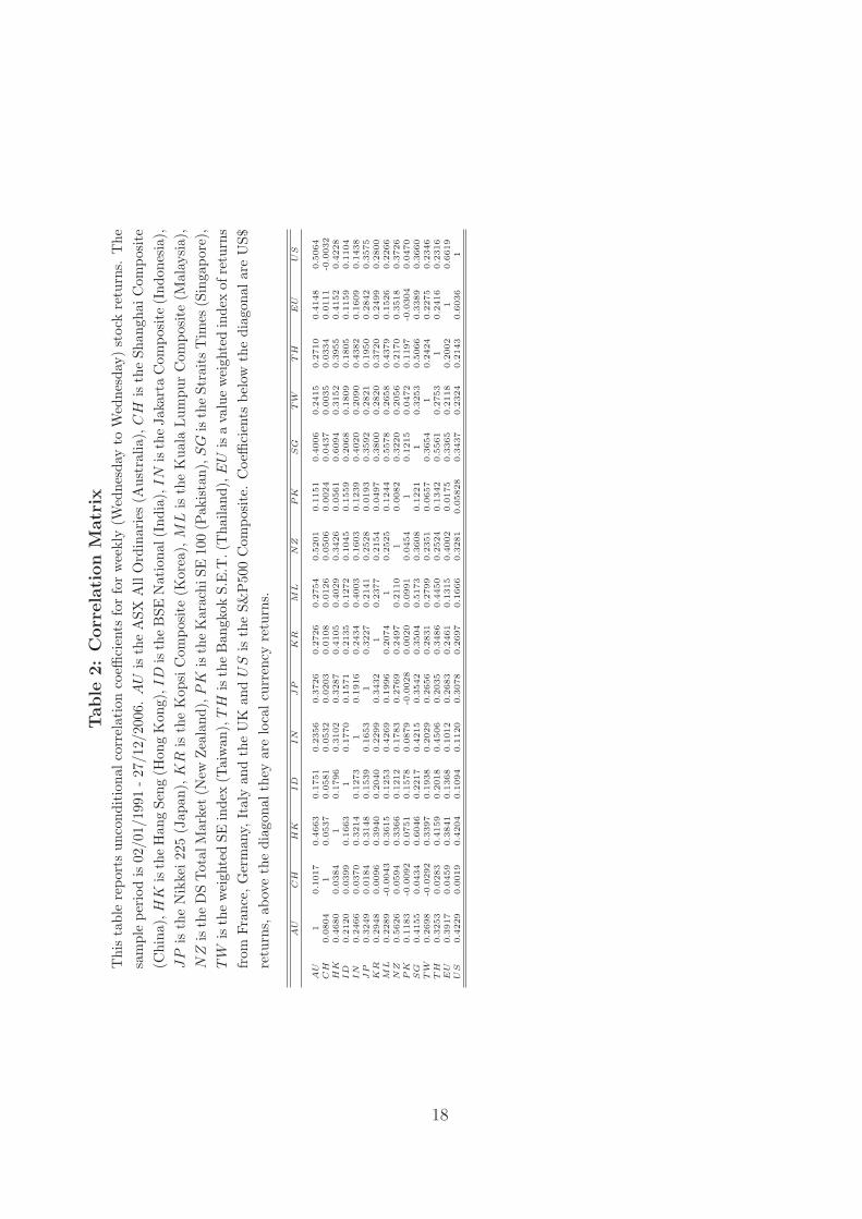
Table 2 reports the unconditional correlations between returns in both local currency and US
dollar terms. China and Pakistan have much lower correlations with the other markets, with means
of 0.03 and 0.07 respectively in both local currency and US dollar terms. India has a mean correlation
around 0.15 while all other markets are moderately correlated with mean correlations in the range
0.22 to 0.35.3 As would be expected the correlations with the US and the European markets relative
to Australia, Hong Kong, Japan, New Zealand and Thailand are quite high. While the correlations
for China, India, Indonesia, Malaysia and Pakistan are considerably smaller. Our results also take
account of foreign exchange movements and the impact that this may have on the correlations. The
table highlights that estimated correlations are different for local currency and US dollar returns
for each market, accounting for currency variations has a significant although not systematic affect
on correlation. This appears to particularly the case for countries with low correlations with the US
and Europe, namely China, India, Indonesia and Pakistan. For example, the correlation between
Malaysia and the US moves from 0.23 in local currency to 0.17 in US dollar terms, for a period
2China, Malaysia and Singapore have positively skewed local currency returns, while China, Japan and Thailand
have positively skewed US dollar returns.3The median correlation is (excluding China, India and Pakistan) 0.23 (0.28).
7

where the ringgit was pegged to the US dollar for a number of years during the current sample.
The first stage of the estimation process is to fit univariate GARCH specifications for each
of the 15 return series. To account for possible asymmetry in conditional volatility we estimate
EGARCH models in each case. We find evidence of asymmetry in most of the stock markets under
investigation. It appears that there is very little evidence of asymmetry for a large number of the
emerging markets. In particular markets that have low correlations with the US (and Europe)
provide very little evidence of volatility feedback, namely China, India and Indonesia. This is the
case for both local and US dollar returns.4,5 Parameter estimates from the univariate EGARCH
models are reported in Table 3. Figure 2 plots news impact curves for 3 of the Asian markets
(Korea, Malaysia and Thailand) in addition to the EU and the US for both hedged and unhedged
returns. For those markets with significant volatility feedback, the curves provide clear evidence of
an asymmetric response to bad news. Similarly in the case of Thailand the curves reinforce the lack
of asymmetry findings of Table 3.
Given the large literature on the Asian crisis and contagion, we consider the possibility that
the crisis period represented a structural break due to the large number of Asia-Pacific (and wider)
markets effected. To account for this, we test for the existence of a structural break in the intercept.
We also consider two alternate crisis dates: 02/07/1997 when the Thai Baht devalued and the crisis
commenced, and 22/10/1997 when there were devaluations of the Taiwanese dollar and Korean
won and a large fall in the Hong Kong equity market, representing the widening of the crisis. Table
4 reports the log-likelihood values from a series of models. The likelihood ratio tests reject the
null hypothesis of no structural break in mean, indicating that all the models allowing for a mean
break significantly outperform the non-break models. Similarly, all the asymmetric generalised
DCC models outperform the non-asymmetric models. These results are supported by the BIC
results. Moreover, in both local currency and US dollar models, adopting a break at 22/10/1997
(the widening of the crisis) rather than 02/07/1997 (when the crisis commenced) reduces the BIC,
implying that 22/10/1997 is a more preferable break date for the crisis. We therefore report our
4Indeed, in some cases (China, India, New Zealand and Pakistan) we find the “good news” chasing effect docu-
mented in emerging markets, however, the positive asymmetry coefficient is typically always statistically insignificant.5Evidence of asymmetry is much weaker for the hedged (US dollar) returns.
8
results for the AG-DCC-GARCH model with a mean break at 22/10/1997.6
The parameter estimates of the AG-DCC-GARCH model are reported in Table 5. Most parame-
ter coefficients are statistically significant at conventional levels. In all cases except China, India and
Indonesia we find evidence of asymmetries in conditional correlations. The conditional correlations
and conditional covariances for local currency returns estimated from the AG-DCC-GARCH model
with a mean break are plotted in Figure 3 for the correlations and covariances of the 14 markets
with the US and Figure 4 for the correlations and covariances of the 13 markets with the EU. While
correlations indicate the relationship between two returns, the covariance captures the amount of
comovement between them. Thus it is possible to determine whether changes in comovement are
due to a change in the correlations between markets or simply due to volatility. Figure 5 provides
plots of the conditional correlations and conditional covariances between the 5 markets central to
the Asian crisis; Indonesia, Korea, Malaysia, Taiwan and Thailand.7 On each plot the break date
of 22/10/97 is marked with a vertical line, while the shaded area corresponds to the Asian crisis
period 02/07/97 - 30/12/98. There is clear evidence of considerable variation in correlations and
covariances in all cases. Typically the dynamic pattern of correlations is also witnessed in the
corresponding covariances, although variation in volatility leads to periods of significantly different
behaviour. There is evidence of further global market integration toward the end of the sample
period, since correlations rise while covariances tend to fall as a consequence of decreasing volatility.
Correlations of Asia-Pacific countries with the US and the EU provide no clear pattern across
the Asian crisis period. Indeed, consistent with Longin and Solnik (2001) and Ang and Bekaert
(2002), analysing the time varying conditional correlations highlights that correlations with the US
and the EU tend to increase and reach a maximum during the recent bear market between 2000
and 2003. Further, correlations tend to be higher post 2001 than in the early part of the sample,
despite reduced correlations due to the bull market post 2003, suggesting greater equity market
integration. This is particularly the case for newer emerging markets in the region such as China
and India, although developed markets such as Japan also witness significantly higher correlations
6Aside from poorer in-sample performance, qualitatively the results do not change if a break date of 02/07/97 is
adopted.7We select these as the correlations and covariances to report and discuss, plots of all 105 local currency and all
105 US dollar correlations and covariances are available from the authors on request.
9

toward the end of the sample.
In contrast to correlations with the US and the EU, Figure 5 clearly shows a large increase in
correlation among the 5 Asian crisis countries at the onset of the crisis. In most cases we witness
correlations falling after the end of the crisis, yet correlations levels seem to remain higher than
pre-crisis levels. The majority of correlations with Malaysia, Taiwan and Thailand in both local
currency and US dollars, and with Indonesia and Korea in US dollars peak during the crisis period.8
The results show that the Asian crisis caused a significant increase in intra-regional correlations.
However no such impact was witnessed with respect to correlations with the US and Europe.
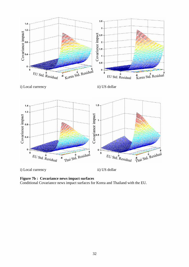
To investigate further the impact of the observed asymmetries, we examine the news impact
surfaces of Kroner and Ng (1998). Figures 6a, 6b and 6c plot the correlation news impact surfaces
for Korea and Thailand with the US (6a), Europe (6b) and between themselves and Malaysia (6c)
for both local currency and US dollar returns. The asymmetry in correlation to joint bad and joint
good news is clearly visible in virtually all cases. The correlation news impact surface reveals a
much larger response in the negative-negative (-/-) quadrant than in the positive-positive (+/+)
quadrant. Hence the impact observed when negative shocks (bad news) occur simultaneously in
both markets is higher than for joint positive shocks (good news) for both unhedged local currency
returns and hedged US dollar returns. The effect is strongest for correlations with the US and
Europe, while its presence is virtually undetectable for US dollar return correlations with Malaysia.
This correspond with the relatively high levels of asymmetry reported in Table 5 for the US and
the lack of asymmetry for Malaysia. The effect of asymmetry becomes even more striking when
we examine the covariance news impact surfaces (Figures 7a, 7b and 7c). The combination of the
correlation with the two conditional volatilities produces a huge increase in the -/- quadrant. The
increase witnessed in response to joint good news is typically much lower. There is little evidence of
asymmetry in the +/- and -/+ quadrants for covariances with the US and Europe, however these
asymmetries are visible in covariances between Asia-Pacific markets.
8The results highlight that correlations with New Zealand peak in virtually every case during the Asian crisis
(22/28 cases).
10

5 Conclusion
In this paper we investigate correlation dynamics between 13 Asia-Pacific stock markets, the EU
and the US. Correlations are key to international portfolio diversification and asset allocation deci-
sions. While most of previous literature on volatility transmission only concentrates on covariance
between markets, we provide a more comprehensive view showing both dynamic covariance and
dynamic correlation between asset prices across markets. Using the recently developed asymmetric
generalised dynamic conditional correlation GARCH model (AG-DCC-GARCH) of Cappiello et al.
(2006) we examine how conditional correlations and covariances for both local currency and hedged
US Dollar returns evolve over time. We uncover evidence of wide variation in correlations through
time, with conditional correlations deviating significantly from the levels of unconditional correla-
tions. Importantly, we also establish significant asymmetry in correlations between many markets.
Reinforcing the established view that correlations increase in response to bad news, crisis events,
bear markets. Although importantly there seems to be little asymmetry in countries that are not
highly correlated with developed markets, suggesting a link between levels of market integration
and volatility feedback.
Incorporating a structural break due to the Asian crisis at 22/10/97 improves the fit of the
estimated model. However, significantly, increases in conditional correlations during the Asian crisis
seem to be mainly limited to crisis countries in the region, correlations involving other markets are
not systematically effected. Although correlations with the US and Europe are relatively immune
to the crisis, they do rise during the bear market in the early 2000s. In addition we document a
general increase in correlations over the entire sample period indicative of greater global market
integration.
Further we demonstrate the asymmetric response of both conditional correlations and covari-
ances to join bad and good news highlighting that the impact of crises and bear markets on corre-
lation are further compounded by volatility. These findings throw further light on correlation and
covariance dynamics between equity markets. These dynamics highlight substantial time variation
in international portfolio diversification opportunities across the Asia-Pacific, EU and US markets.
11

References
Ang, A. and G. Bekaert 2002, “International asset allocation with regime shifts”, Review of Financial
Studies, 15, 1137-1187.
Bae, K.-H., G.A. Karolyi and R.M. Stulz 2003, “A new approach to measuring financial contagion”,
Review of Financial Studies, 16, 717-763.
Baele, L., ‘Volatility Spillover Effects in European Equity Markets’, Journal of Financial and Quan-
titative Analysis, Vol. 40, 2005, pp. 373-401.
Bekaert, G. and C.R. Harvey 1995, “Time-varying world market integration”, Journal of Finance,
50, 403-444.
Bekaert, G. and C.R. Harvey 1997, “Emerging equity market volatility”, Journal of Financial
Economics, 43, 29-77.
Cappiello, L., R.F. Engle and K. Sheppard 2006, “Asymmetric dynamics in the correlations of global
equity and bond returns”, Journal of Financial Econometrics, 4, 537-572.
Cha, B. and Y.-L. Cheung 1998, “The impact of the US and the Japanese equity markets on the
emerging Asia-Pacific equity markets”, Asia-Pacific Financial Markets, 5, 191-209.
Chan, K.C., B.E. Gup and M. Pan 1992, “An empirical analysis of stock prices in major Asian
markets and the United States”, Financial Review, 27, 289-307.
Darrat, A.F. and M. Zhong 2002, “Permanent and transitory driving forces in Asian-Pacific stock
markets”, Financial Review, 31, 343-363.
Edwards, S. and R. Susmel 2001, “Volatility dependence and contagion in emerging equity markets”,
Journal of Development Economics, 66, 505-532.
Engle, R.F. 2002, “Dynamic conditional correlation: A simple class of multivariate generalized
autoregressive-conditional heteroskedasticity models”, Journal of Business and Economic Statis-
tics, 20, 339-350.
12

Engle, R.F., T. Ito and W.-L. Lin 1990, “Meteor showers or heat waves? Heterskedastic intra-daily
volatility in the foreign exchange market”, Econometrica, 58, 525-542.
Engle, R.F. and K. Sheppard 2001, “Theoretical and empirical properties of Dynamic Conditional
Correlation MVGARCH”, Working paper No. 2001-15, University of California, San Diego.
Erb, C.B., C.R. Harvey and T.E. Viskanta 1994, “Forecasting international equity correlations”,
Financial Analysts Journal, 50, 32-45.
Garrett, I. and S. Spyrou 1999, “Common stochastic trends in emerging equity markets”, The
Manchester School, 67, 649-660.
Ghosh, A., R. Saidi and K.H. Johnson 1999, “Who moves the Asia-Pacific stock markets - US or
Japan?”, Financial Review, 34, 159-169.
Goetzmann, W.N., L. Li and K.G. Rouwenhorst 2005, “Long-term global market correlations”,
Journal of Business, 78, 1-38.
Hamao, Y., R. Masulis and V. Ng 1990, “Correlation in price changes and volatility across interna-
tional stock markets”, Review of Financial Studies, 3, 281-307.
Janakiramanan, S. and A. Lamba 1998, “An empirical investigation of linkages between Pacific-
Basin stock markets”, Journal of International Financial Markets, Institutions and Money, 8,
155-173.
Kasa, K. 1992, “Common stochastic trends in international stock markets”, Journal of Monetary
Economics, 29, 95-124.
Kaminsky, G.L. and C.M. Reinhart 1998, “Financial crises in Asia and Latin America”, American
Economic Review, 88, 444-448.
Kim, S. 2005, “Informational leadership in the advancd Asia-Pacific stock markets: Return, volatil-
ity and volume information spillovers from the US and Japan”, Journal of Japanese and Inter-
national Economics, 19, 338-365.
13

Kroner, K.F. and V.K. Ng 1998, “Modelling asymmetric comovements of asset returns”, Review of
Financial Studies, 11, 817-844.
Longin, F. and B. Solnik, 1995, “Is the Correlation in International Equity Returns Constant”,
Journal of International Money and Finance, 14, 3-26.
Longin, F. and B. Solnik 2001, “Extreme correlation and international equity markets”, Journal of
Finance, 56, 649-676.
Maish, A.M.M. and R. Maish 1999, “Are Asian stock market fluctuations due mainly to intra-
regional contagion effects? Evidence based on Asian emerging markets”, Pacific-Basin Finance
Journal, 7, 251-282.
Manning, N. 2002, “Common trends and convergence? South East Asian equity markets 1988-
1999”, Journal of International Money and Finance, 21, 183-202.
Ng., A. 2000, “Volatility spillover effects from Japan and the US to the Pacific-Basin”, Journal of
International Money and Finance, 19, 207-233.
Phylaktis, K. 1999, “Capital market integration in the Pacific Basin region: an impulse response
analysis”, Journal of International Money and Finance, 18, 267-287.
Phylaktis K. and F. Ravazzolo 2002, “Measuring financial and economic integration with equity
prices in emerging markets”, Journal of International Money and Finance, 21, 879-903.
Worthington, A. and H. Higgs 1004, “Transmission of equity returns and volatility in Asian devel-
oped and emerging markets: A Multivariate GARCH analysis” International Journal of Finance
and Economics, 9, 71-80.
Yang, J., J.W. Kolari and I. Min 2003, “Stock market integration and financial crises: the case of
Asia”, Applied Financial Economics, 13, 477-486.
Yang, J., J.W. Kolari and P.W. Sutanto 2004, “On the stability of long-run relationships between
emerging and US stock markets”, Journal of Multinational Financial Management, 14, 233-248.
14

A Maximum likelihood estimation of AG-DCC-MVGARCH
model
Engle (2002) and Engle and Sheppard (2001) propose the two-step estimation of DCC-MVGARCH
model:
rt|Ωt−1 ∼ N(0, Ht) ∼ N(0, DtRtDt)
The normality assumption of rt gives rise to a log-likelihood function. Without the normality
assumption, the estimator will still have the Quasi-Maximum Likelihood (QML) interpretation.
The log likelihood for this estimator can be written as:
L = −12
T∑t=1
(n log(2π) + log |Ht|+ r′tH
−1t rt
)
−12
T∑t=1
(n log(2π) + log |DtRtDt|+ r′tD
−1t R−1
t D−1t rt
)
Since the standardized residual, εt = rt√ht
= D−1t rt, the log-likelihood function can be expressed
as:
L = −12
T∑t=1
(n log(2π) + 2 log |Dt|+ log |Rt|+ ε′tR
−1t εt
)
−12
T∑t=1
(n log(2π) + 2 log |Dt|+ r′tD
−1t D−1
t rt − ε′tεt + log |Rt|+ ε′tR−1t εt
)
It is clear that there are two separate parts of the log-likelihood function, the volatility part
containing Dt and the correlation part containing Rt. This gives rise to the two stage estimation
procedure. In the first stage, each of Dt can be considered as an univariate GARCH model, therefore
the log-likehood of the volatility term is simply the sum of the log-likelihoods of the individual
GARCH equations for the assets:
15
L = −12
T∑t=1
(n log(2π) + 2 log |Dt|+ r′tD
−1t D−1
t rt
)
−12
T∑t=1
(n log(2π) + 2 log |Dt|+ r′tD
−2t rt
)
−12
T∑t=1
(n log(2π) +
n∑i=1
(log(hit) +
r2it
hit
))
−12
n∑i=1
(T log(2π) +
T∑t=1
(log(hit) +
r2it
hit
))
In the second stage, the DCC parameters are estimated using the specified log-likehood of the
correlation part, conditioning on the parameters estimated in the first stage likelihood:
LC = −1
2
T∑t=1
(log |Rt|+ ε′tR
−1t εt − ε′tεt
)
It should be noted that the two-step estimation of the likelihood function means that estimation
is inefficient, though consistent (Engle and Sheppard, 2001; Engle, 2002).
16

Table 1: Summary StatisticsThis table reports summary statistics for weekly (Wednesday to Wednesday)stock returns. The sample period is 02/01/1991 - 27/12/2006. AU is theASX All Ordinaries (Australia), CH is the Shanghai Composite (China), HK
is the Hang Seng (Hong Kong), ID is the BSE National (India), IN is theJakarta Composite (Indonesia), JP is the Nikkei 225 (Japan), KR is the KopsiComposite (Korea), ML is the Kuala Lumpur Composite (Malaysia), NZ isthe DS Total Market (New Zealand), PK is the Karachi SE 100 (Pakistan),SG is the Straits Times (Singapore), TW is the weighted SE index (Taiwan),TH is the Bangkok S.E.T. (Thailand), EU is a value weighted index of returnsfrom France, Germany, Italy and the UK and US is the S&P500 Composite. *indicates significance at 1 percent.
Series Mean Median Std. Dev. Skewness Kurtosis Jarque-BeraPanel A: Local currency returnsAU 0.0783 0.0809 0.7297 -0.2761 4.3363 43.84*CH 0.1550 0.1148 2.5187 2.1910 28.601 813.36*HK 0.0969 0.1736 1.4394 -0.5130 4.7359 56.716*ID 0.1343 0.2783 1.7484 0.0412 6.2278 190.38*IN 0.0778 0.1643 1.5015 -0.0892 5.3233 114.66*JP -0.0170 0.0189 1.2763 -0.0040 4.1727 38.348*KR 0.0373 0.0212 1.7721 -0.1142 4.8708 80.917*ML 0.0400 0.0562 1.5001 0.4260 12.3453 743.54*NZ -0.0670 0.0809 0.9003 -0.0979 6.7182 232.45*PK 0.1472 0.2019 1.7280 -0.3452 5.0762 83.644*SG 0.0603 0.0407 1.2476 0.0069 5.6091 138.47*TW 0.0308 0.0686 1.6428 -0.1990 4.9570 83.962*TH 0.0070 0.0615 1.7356 0.1723 4.3554 47.030*EU 0.0653 0.1244 0.8981 -0.4187 6.1587 152.79*US 0.0760 0.1292 0.9031 -0.1164 5.1680 102.16*Panel B: US Dollar returnsAU 0.0796 0.1740 0.9840 -0.3378 3.4653 16.213*CH 0.1336 0.1232 2.6240 1.5121 25.047 1254.6*HK 0.0971 0.1860 1.4474 -0.5121 4.6811 54.485*ID 0.0879 0.1945 1.8118 -0.3037 5.5440 119.20*IN -0.0028 0.0000 2.4154 -0.8054 13.7600 528.74*JP -0.0099 -0.0040 1.4114 0.0929 4.1730 37.996*KR 0.0237 0.0000 2.1223 -0.7821 10.0035 378.44*ML 0.0262 0.0571 1.8264 -0.9958 21.203 1363.8*NZ 0.0766 0.1825 1.1239 -0.3735 5.6568 120.84*PK 0.0935 0.1780 1.7420 -0.3583 5.0629 81.921*SG 0.0668 0.0642 1.3284 -0.1541 5.9226 160.09*TW 0.0210 0.1005 1.7432 -0.2567 4.9055 77.809*TH -0.0111 0.0163 1.9437 0.0655 5.1981 105.66*EU 0.0707 0.0943 0.9008 -0.4395 5.3717 95.049*
17
Table
2:
Corr
ela
tion
Matr
ixT
his
tabl
ere
port
sun
cond
itio
nalc
orre
lati
onco
effici
ents
for
for
wee
kly
(Wed
nesd
ayto
Wed
nesd
ay)
stoc
kre
turn
s.T
hesa
mpl
epe
riod
is02
/01/
1991
-27
/12/
2006
.A
Uis
the
ASX
All
Ord
inar
ies
(Aus
tral
ia),
CH
isth
eSh
angh
aiC
ompo
site
(Chi
na),
HK
isth
eH
ang
Seng
(Hon
gK
ong)
,ID
isth
eB
SEN
atio
nal(
Indi
a),I
Nis
the
Jaka
rta
Com
posi
te(I
ndon
esia
),JP
isth
eN
ikke
i225
(Jap
an),
KR
isth
eK
opsi
Com
posi
te(K
orea
),M
Lis
the
Kua
laLum
pur
Com
posi
te(M
alay
sia)
,N
Zis
the
DS
Tot
alM
arke
t(N
ewZea
land
),P
Kis
the
Kar
achi
SE10
0(P
akis
tan)
,SG
isth
eSt
rait
sT
imes
(Sin
gapo
re),
TW
isth
ew
eigh
ted
SEin
dex
(Tai
wan
),T
His
the
Ban
gkok
S.E
.T.(
Tha
iland
),E
Uis
ava
lue
wei
ghte
din
dex
ofre
turn
sfr
omFr
ance
,Ger
man
y,It
aly
and
the
UK
and
US
isth
eS&
P50
0C
ompo
site
.C
oeffi
cien
tsbe
low
the
diag
onal
are
US$
retu
rns,
abov
eth
edi
agon
alth
eyar
elo
calcu
rren
cyre
turn
s.
AU
CH
HK
ID
IN
JP
KR
ML
NZ
PK
SG
TW
TH
EU
US
AU
10.1
017
0.4
663
0.1
751
0.2
356
0.3
726
0.2
726
0.2
754
0.5
201
0.1
151
0.4
006
0.2
415
0.2
710
0.4
148
0.5
064
CH
0.0
804
10.0
537
0.0
581
0.0
532
0.0
203
0.0
108
0.0
126
0.0
506
0.0
024
0.0
437
0.0
035
0.0
334
0.0
111
-0.0
032
HK
0.4
680
0.0
384
10.1
796
0.3
102
0.3
287
0.4
105
0.4
029
0.3
426
0.0
561
0.6
094
0.3
152
0.3
955
0.4
152
0.4
228
ID
0.2
120
0.0
399
0.1
663
10.1
770
0.1
571
0.2
135
0.1
272
0.1
045
0.1
559
0.2
068
0.1
809
0.1
805
0.1
159
0.1
104
IN
0.2
466
0.0
370
0.3
214
0.1
273
10.1
916
0.2
434
0.4
003
0.1
603
0.1
239
0.4
020
0.2
090
0.4
382
0.1
609
0.1
438
JP
0.3
249
0.0
184
0.3
148
0.1
539
0.1
653
10.3
227
0.2
141
0.2
528
0.0
193
0.3
592
0.2
821
0.1
950
0.2
842
0.3
575
KR
0.2
948
0.0
096
0.3
940
0.2
040
0.2
299
0.3
432
10.2
377
0.2
154
0.0
497
0.3
800
0.2
820
0.3
720
0.2
499
0.2
800
ML
0.2
289
-0.0
043
0.3
615
0.1
253
0.4
269
0.1
996
0.2
074
10.2
525
0.1
244
0.5
578
0.2
658
0.4
379
0.1
526
0.2
266
NZ
0.5
626
0.0
594
0.3
366
0.1
212
0.1
783
0.2
769
0.2
497
0.2
110
10.0
082
0.3
220
0.2
056
0.2
170
0.3
518
0.3
726
PK
0.1
183
-0.0
092
0.0
751
0.1
578
0.0
879
-0.0
028
0.0
020
0.0
991
0.0
454
10.1
215
0.0
472
0.1
197
-0.0
304
0.0
470
SG
0.4
155
0.0
434
0.6
046
0.2
217
0.4
215
0.3
542
0.3
504
0.5
173
0.3
608
0.1
221
10.3
253
0.5
066
0.3
389
0.3
660
TW
0.2
698
-0.0
292
0.3
397
0.1
938
0.2
029
0.2
656
0.2
831
0.2
799
0.2
351
0.0
657
0.3
654
10.2
424
0.2
275
0.2
346
TH
0.3
253
0.0
283
0.4
159
0.2
018
0.4
506
0.2
035
0.3
486
0.4
450
0.2
524
0.1
342
0.5
561
0.2
753
10.2
416
0.2
316
EU
0.3
917
0.0
459
0.3
841
0.1
368
0.1
012
0.2
683
0.2
461
0.1
315
0.4
002
0.0
175
0.3
365
0.2
118
0.2
002
10.6
619
US
0.4
229
0.0
019
0.4
204
0.1
094
0.1
120
0.3
078
0.2
697
0.1
666
0.3
281
0.0
5828
0.3
437
0.2
324
0.2
143
0.6
036
1
18

Table 3: Univariate Asymmetric GARCH modelsThis table reports parameter estimates for the univariate EGARCH modelsfor weekly (Wednesday to Wednesday) stock returns. The sample period is02/01/1991 - 27/12/2006. AU is the ASX All Ordinaries (Australia), CH isthe Shanghai Composite (China), HK is the Hang Seng (Hong Kong), ID isthe BSE National (India), IN is the Jakarta Composite (Indonesia), JP is theNikkei 225 (Japan), KR is the Kopsi Composite (Korea), ML is the KualaLumpur Composite (Malaysia), NZ is the DS Total Market (New Zealand),PK is the Karachi SE 100 (Pakistan), SG is the Straits Times (Singapore),TW is the weighted SE index (Taiwan), TH is the Bangkok S.E.T. (Thailand),EU is a value weighted index of returns from France, Germany, Italy and theUK and US is the S&P500 Composite. * indicates parameters insignificant at5%.
Panel A: Local currency returns Panel B: US Dollar returnsSeries ω α β γ ω α β γAU -0.2074 0.1928 0.9230 -0.1185 -0.0360* 0.0214* 0.7304 -0.1636CH -0.2598 0.3901 0.9747 0.0380* -0.2693 0.4079 0.9747 0.0303*HK -0.1350 0.1802 0.9858 -0.0023* -0.1389 0.1849 0.9855 -0.0024*ID -0.2058 0.3936 0.9000 0.0003* -0.0938* 0.3404 0.8510 -0.0411*IN -0.0866 0.1289 0.9834 -0.0103* -0.1444 0.2150 0.9848 -0.0232*JP -0.0909 0.1395 0.9505 -0.0933 -0.1046 0.1602 0.9627 -0.0872KR -0.0686 0.0942 0.9921 -0.0467 -0.1093 0.1648 0.9813 -0.0669ML -0.1941 0.2625 0.9797 -0.0353 -0.1888 0.2599 0.9913 -0.0080*NZ -0.1226 0.1550 0.9833 0.0424 -0.1525 0.2082 0.9424 0.0011*PK -0.1828 0.4597 0.8267 0.0085* -0.1619 0.4449 0.8223 0.0100*SG -0.1449 0.1940 0.9723 -0.0465 -0.1414 0.1937 0.9745 -0.0405TW -0.1698 0.2697 0.9485 -0.0306* -0.1521 0.2704 0.9362 -0.0378*TH -0.0766 0.1098 0.9886 -0.0062* -0.0811 0.1217 0.9863 -0.0131*EU -0.1672 0.1816 0.9425 -0.0982 -0.2038 0.2348 0.9439 -0.0757US -0.1441 0.1612 0.9582 -0.1129 -0.1441 0.1612 0.9582 -0.1129
19

Table 4: Log-likelihood valuesThis table reports log-likelihood values for six estimated DCC GARCH modelsfor both local currency returns and US Dollar returns. DCC is the DynamicConditional Correlation, AG−DCC is Asymmetric Generalized Dynamic Con-ditional Correlation. We test for a break due to the Asian Crisis, at 02/07/1997when the Thai Baht devalued (commencement of the crisis) and 22/10/1997when the Taiwanese Dollar and Korean Won devalued and the Hong Kongstock market fell (crisis spreads throughout the region).
Log-likelihood No. of parameters inModel Value the correlation evolution BICPanel A: Local currency returnsDCC -16191.5 105 + 2 39.644DCC w/ mean break at 02/07/1997 -15811.1 210 + 2 39.578DCC w/ mean break at 22/10/1997 -15802.3 210 + 2 39.557
AG−DCC -15792.6 105 + 102 39.494AG−DCC w/ mean break at 02/07/1997 -15427.3 210 + 102 39.465AG−DCC w/ mean break at 22/10/1997 -15418.1 210 + 102 39.443Panel B: US Dollar returnsDCC -16130.4 105 + 2 39.497DCC w/ mean break at 02/07/1997 -15702.3 210 + 2 39.318DCC w/ mean break at 22/10/1997 -15981.6 210 + 2 39.292
AG−DCC -16001.3 105 + 102 39.994AG−DCC w/ mean break at 02/07/1997 -15646.1 210 + 102 39.989AG−DCC w/ mean break at 22/10/1997 -15633.6 210 + 102 39.959
20
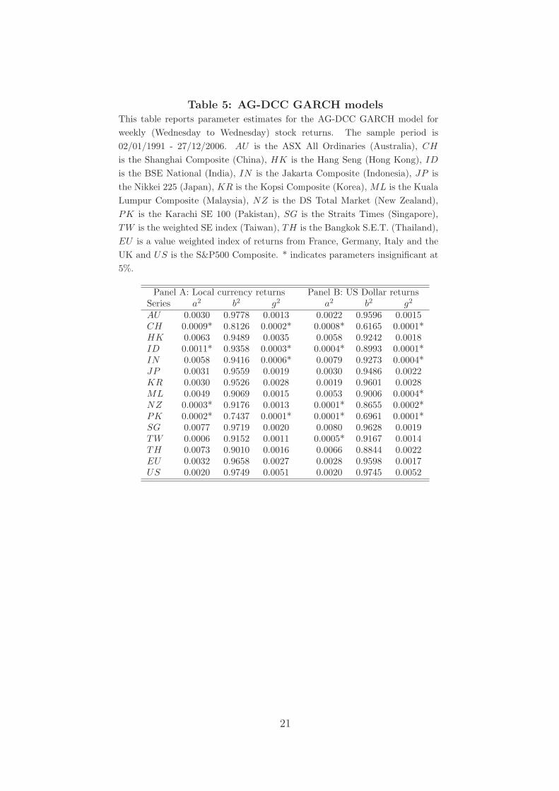
Table 5: AG-DCC GARCH modelsThis table reports parameter estimates for the AG-DCC GARCH model forweekly (Wednesday to Wednesday) stock returns. The sample period is02/01/1991 - 27/12/2006. AU is the ASX All Ordinaries (Australia), CH
is the Shanghai Composite (China), HK is the Hang Seng (Hong Kong), ID
is the BSE National (India), IN is the Jakarta Composite (Indonesia), JP isthe Nikkei 225 (Japan), KR is the Kopsi Composite (Korea), ML is the KualaLumpur Composite (Malaysia), NZ is the DS Total Market (New Zealand),PK is the Karachi SE 100 (Pakistan), SG is the Straits Times (Singapore),TW is the weighted SE index (Taiwan), TH is the Bangkok S.E.T. (Thailand),EU is a value weighted index of returns from France, Germany, Italy and theUK and US is the S&P500 Composite. * indicates parameters insignificant at5%.
Panel A: Local currency returns Panel B: US Dollar returnsSeries a2 b2 g2 a2 b2 g2
AU 0.0030 0.9778 0.0013 0.0022 0.9596 0.0015CH 0.0009* 0.8126 0.0002* 0.0008* 0.6165 0.0001*HK 0.0063 0.9489 0.0035 0.0058 0.9242 0.0018ID 0.0011* 0.9358 0.0003* 0.0004* 0.8993 0.0001*IN 0.0058 0.9416 0.0006* 0.0079 0.9273 0.0004*JP 0.0031 0.9559 0.0019 0.0030 0.9486 0.0022KR 0.0030 0.9526 0.0028 0.0019 0.9601 0.0028ML 0.0049 0.9069 0.0015 0.0053 0.9006 0.0004*NZ 0.0003* 0.9176 0.0013 0.0001* 0.8655 0.0002*PK 0.0002* 0.7437 0.0001* 0.0001* 0.6961 0.0001*SG 0.0077 0.9719 0.0020 0.0080 0.9628 0.0019TW 0.0006 0.9152 0.0011 0.0005* 0.9167 0.0014TH 0.0073 0.9010 0.0016 0.0066 0.8844 0.0022EU 0.0032 0.9658 0.0027 0.0028 0.9598 0.0017US 0.0020 0.9749 0.0051 0.0020 0.9745 0.0052
21

1991 1994 1997 2000 2003 2006−5.0
−2.5
0.0
2.5Australia
1991 1994 1997 2000 2003 2006−15
0
15
30 China
1991 1994 1997 2000 2003 2006
−5
0
5Hong Kong
1991 1994 1997 2000 2003 2006
−5
0
5
10India
1991 1994 1997 2000 2003 2006
−5
0
5Indonesia
1991 1994 1997 2000 2003 2006−5
0
5
Japan
1991 1994 1997 2000 2003 2006
−5
0
5Korea
1991 1994 1997 2000 2003 2006−10
0
10
Malaysia
Figure 1: Stock Returns
Weekly (Wednesday to Wednesday) local currency returns from 03/01/1991 to 28/12/2006.
22

1991 1994 1997 2000 2003 2006−5
0
5 New Zealand
1991 1994 1997 2000 2003 2006
−5
0
5
Pakistan
1991 1994 1997 2000 2003 2006
−5
0
5Singapore
1991 1994 1997 2000 2003 2006
−5
0
5Taiwan
1991 1994 1997 2000 2003 2006
−5
0
5
10 Thailand
1991 1994 1997 2000 2003 2006−5.0
−2.5
0.0
2.5
5.0 EU
1991 1994 1997 2000 2003 2006−5.0
−2.5
0.0
2.5
5.0 US
Figure 1 (cont.): Stock Returns
Weekly (Wednesday to Wednesday) local currency returns from 03/01/1991 to 28/12/2006.
23

Figure 2 : News Impact Curves News impact curves from univariate asymmetric GARCH models (for both local currency and US dollar returns) for Korea, Malaysia, Thailand, the EU and the US.
24

AUSTRALIA & US
1991 1993 1995 1997 1999 2001 2003 20050.450
0.475
0.500
0.525
0.550
0.575
0.600
0.1
0.2
0.3
0.4
0.5
0.6
0.7
0.8
0.9
Corr
CHINA & US
1991 1993 1995 1997 1999 2001 2003 2005-0.050
-0.025
0.000
0.025
0.050
-0.36
-0.24
-0.12
0.00
0.12
0.24
Corr
HONG KONG & US
1991 1993 1995 1997 1999 2001 2003 20050.34
0.36
0.38
0.40
0.42
0.44
0.46
0.48
0.00
0.25
0.50
0.75
1.00
1.25
1.50
1.75
2.00
Corr
INDIA & US
1991 1993 1995 1997 1999 2001 2003 2005-0.04
0.00
0.04
0.08
0.12
0.16
0.20
0.24
-0.2
0.0
0.2
0.4
0.6
0.8
1.0
Corr
INDONESIA & US
1991 1993 1995 1997 1999 2001 2003 20050.0720.0900.1080.1260.1440.1620.1800.1980.2160.234
0.00.10.20.30.40.50.60.70.80.9
Corr
JAPAN & US
1991 1993 1995 1997 1999 2001 2003 20050.30
0.32
0.34
0.36
0.38
0.40
0.42
0.44
0.0
0.2
0.4
0.6
0.8
1.0
1.2
Corr
KOREA & US
1991 1993 1995 1997 1999 2001 2003 20050.200
0.225
0.250
0.275
0.300
0.325
0.350
0.0
0.2
0.4
0.6
0.8
1.0
1.2
Corr
MALAYSIA & US
1991 1993 1995 1997 1999 2001 2003 20050.150
0.175
0.200
0.225
0.250
0.275
0.300
0.325
0.00
0.25
0.50
0.75
1.00
1.25
1.50
1.75
Corr
NEW ZEALAND & US
1991 1993 1995 1997 1999 2001 2003 20050.30
0.32
0.34
0.36
0.38
0.40
0.42
0.44
0.46
0.0
0.2
0.4
0.6
0.8
1.0
1.2
Corr
PAKISTAN & US
1991 1993 1995 1997 1999 2001 2003 2005-0.016
0.000
0.016
0.032
0.048
0.064
0.080
0.096
0.112
-0.050.000.050.100.150.200.250.300.350.40
Corr
SINGAPORE & US
1991 1993 1995 1997 1999 2001 2003 20050.28
0.30
0.32
0.34
0.36
0.38
0.40
0.42
0.44
0.00
0.25
0.50
0.75
1.00
1.25
1.50
1.75
Corr
TAIWAN & US
1991 1993 1995 1997 1999 2001 2003 20050.160.180.200.220.240.260.280.300.320.34
0.00
0.25
0.50
0.75
1.00
1.25
1.50
Corr
THAILAND & US
1991 1993 1995 1997 1999 2001 2003 20050.150
0.175
0.200
0.225
0.250
0.275
0.300
0.325
0.0
0.2
0.4
0.6
0.8
1.0
1.2
Corr
US & EU
1991 1993 1995 1997 1999 2001 2003 20050.600
0.625
0.650
0.675
0.700
0.725
0.0
0.5
1.0
1.5
2.0
2.5
3.0
Corr
Figure 3 : Conditional Correlations and Conditional Covariances with US Conditional correlations and covariances for local currency returns. Shaded area corresponds to Asian crisis period 02/07/1997 – 30/12/1998.
Line corresponds to break at 22/10/1997.
25

AUSTRALIA & EU
1991 1993 1995 1997 1999 2001 2003 20050.350
0.375
0.400
0.425
0.450
0.475
0.500
0.1
0.2
0.3
0.4
0.5
0.6
0.7
0.8
0.9
Corr
CHINA & EU
1991 1993 1995 1997 1999 2001 2003 2005-0.04
-0.02
0.00
0.02
0.04
0.06
0.08
0.10
-0.1
0.0
0.1
0.2
0.3
0.4
0.5
0.6
0.7
Corr
HONG KONG & EU
1991 1993 1995 1997 1999 2001 2003 20050.360
0.378
0.396
0.414
0.432
0.450
0.468
0.486
0.000.250.500.751.001.251.501.752.002.25
Corr
INDIA & EU
1991 1993 1995 1997 1999 2001 2003 20050.0000.0250.0500.0750.1000.1250.1500.1750.2000.225
0.0
0.2
0.4
0.6
0.8
1.0
1.2
Corr
INDONESIA & EU
1991 1993 1995 1997 1999 2001 2003 20050.0750.1000.1250.1500.1750.2000.2250.2500.2750.300
0.0
0.2
0.4
0.6
0.8
1.0
1.2
1.4
1.6
Corr
JAPAN & EU
1991 1993 1995 1997 1999 2001 2003 20050.225
0.250
0.275
0.300
0.325
0.350
0.12
0.24
0.36
0.48
0.60
0.72
0.84
0.96
1.08
Corr
KOREA & EU
1991 1993 1995 1997 1999 2001 2003 20050.160.180.200.220.240.260.280.300.320.34
0.0
0.2
0.4
0.6
0.8
1.0
1.2
1.4
Corr
MALAYSIA & EU
1991 1993 1995 1997 1999 2001 2003 20050.0640.0800.0960.1120.1280.1440.1600.1760.1920.208
0.0
0.2
0.4
0.6
0.8
1.0
1.2
1.4
Corr
NEW ZEALAND & EU
1991 1993 1995 1997 1999 2001 2003 20050.30
0.32
0.34
0.36
0.38
0.40
0.42
0.44
0.46
0.0
0.2
0.4
0.6
0.8
1.0
1.2
Corr
PAKISTAN & EU
1991 1993 1995 1997 1999 2001 2003 2005-0.10
-0.08
-0.06
-0.04
-0.02
0.00
0.02
0.04
0.06
-0.7-0.6-0.5-0.4-0.3-0.2-0.1-0.00.10.2
Corr
SINGAPORE & EU
1991 1993 1995 1997 1999 2001 2003 20050.250
0.275
0.300
0.325
0.350
0.375
0.400
0.425
0.450
0.0
0.2
0.4
0.6
0.8
1.0
1.2
1.4
1.6
Corr
TAIWAN & EU
1991 1993 1995 1997 1999 2001 2003 20050.16
0.18
0.20
0.22
0.24
0.26
0.28
0.30
0.32
0.00
0.25
0.50
0.75
1.00
1.25
1.50
Corr
THAILAND & EU
1991 1993 1995 1997 1999 2001 2003 20050.150
0.175
0.200
0.225
0.250
0.275
0.300
0.325
0.0
0.2
0.4
0.6
0.8
1.0
1.2
1.4
Corr
Figure 4 : Conditional Correlations and Conditional Covariances with EU Conditional correlations and covariances for local currency returns. Shaded area corresponds to Asian crisis period 02/07/1997 – 30/12/1998. Line corresponds to break at 22/10/1997.
26

INDONESIA & KOREA
1991 1993 1995 1997 1999 2001 2003 20050.175
0.200
0.225
0.250
0.275
0.300
0.325
0.350
0.0
0.5
1.0
1.5
2.0
2.5
3.0
Corr
INDONESIA & MALAYSIA
1991 1993 1995 1997 1999 2001 2003 20050.350
0.375
0.400
0.425
0.450
0.475
0.500
0.525
0.550
0
1
2
3
4
5
6
Corr
INDONESIA & THAILAND
1991 1993 1995 1997 1999 2001 2003 20050.375
0.400
0.425
0.450
0.475
0.500
0.525
0.0
0.5
1.0
1.5
2.0
2.5
3.0
3.5
4.0
Corr
INDONESIA & TAIWAN
1991 1993 1995 1997 1999 2001 2003 20050.150
0.175
0.200
0.225
0.250
0.275
0.300
0.2
0.4
0.6
0.8
1.0
1.2
1.4
1.6
Corr
MALAYSIA & KOREA
1991 1993 1995 1997 1999 2001 2003 20050.180.200.220.240.260.280.300.320.340.36
0.00.51.01.52.02.53.03.54.04.5
Corr
MALAYSIA & TAIWAN
1991 1993 1995 1997 1999 2001 2003 20050.20
0.22
0.24
0.26
0.28
0.30
0.32
0.34
0.0
0.5
1.0
1.5
2.0
2.5
3.0
3.5
Corr
MALAYSIA & THAILAND
1991 1993 1995 1997 1999 2001 2003 20050.3250.3500.3750.4000.4250.4500.4750.5000.5250.550
0
1
2
3
4
5
6
7
Corr
KOREA & TAIWAN
1991 1993 1995 1997 1999 2001 2003 20050.175
0.200
0.225
0.250
0.275
0.300
0.325
0.350
0.375
0.0
0.4
0.8
1.2
1.6
2.0
2.4
2.8
Corr
KOREA & THAILAND
1991 1993 1995 1997 1999 2001 2003 20050.300
0.325
0.350
0.375
0.400
0.425
0.450
0.00.51.01.52.02.53.03.54.04.5
Corr
TAIWAN & THAILAND
1991 1993 1995 1997 1999 2001 2003 20050.125
0.150
0.175
0.200
0.225
0.250
0.275
0.300
0.325
0.25
0.50
0.75
1.00
1.25
1.50
1.75
2.00
2.25
Corr
Figure 5 : Conditional Correlations and Conditional Covariances between Asian Crisis countries (Indonesia, Korea, Malaysia, Taiwan and Thailand). Conditional correlations and covariances for local currency returns. Shaded area corresponds to Asian crisis period 02/07/1997 – 30/12/1998. Line corresponds to break at 22/10/1997.
27

i) Local currency ii) US dollar
i) Local currency ii) US dollar
Figure 6a : Correlation news impact surfaces Conditional Correlation news impact surfaces for Korea and Thailand with the US.
28

i) Local currency ii) US dollar
i) Local currency ii) US dollar Figure 6b : Correlation news impact surfaces Conditional Correlation news impact surfaces for Korea and Thailand with the EU.
29

i) Local currency ii) US dollar
i) Local currency ii) US dollar
i) Local currency ii) US dollar Figure 6c : Correlation news impact surfaces Conditional Correlation news impact surfaces between Korea, Malaysia and Thailand.
30

i) Local currency ii) US dollar
i) Local currency ii) US dollar
Figure 7a : Covariance news impact surfaces Conditional Covariance news impact surfaces for Korea and Thailand with the US.
31
i) Local currency ii) US dollar
i) Local currency ii) US dollar
Figure 7b : Covariance news impact surfaces Conditional Covariance news impact surfaces for Korea and Thailand with the EU.
32

i) Local currency ii) US dollar
i) Local currency ii) US dollar
i) Local currency ii) US dollar Figure 7c : Covariance news impact surfaces
33Conditional Covariance news impact surfaces between Korea, Malaysia and Thailand.