Embed Size (px)
Citation preview

Cosmology in the Next Decade
Eiichiro KomatsuTexas Cosmology Center, University of Texas at Austin
JGRG, September 28, 2011

Cosmology: Next Decade?• Astro2010: Astronomy & Astrophysics Decadal Survey
• Report from Cosmology and Fundamental Physics Panel (Panel Report, Page T-3):
2

Cosmology: Next Decade?• Astro2010: Astronomy & Astrophysics Decadal Survey
• Report from Cosmology and Fundamental Physics Panel (Panel Report, Page T-3): Translation
InflationDark EnergyDark MatterNeutrino Mass
3

Cosmology Update: WMAP 7-year+
• Standard Model
• H&He = 4.58% (±0.16%)
• Dark Matter = 22.9% (±1.5%)
• Dark Energy = 72.5% (±1.6%)
• H0=70.2±1.4 km/s/Mpc
• Age of the Universe = 13.76 billion years (±0.11 billion years) “ScienceNews” article on
the WMAP 7-year results4

Can we prove/falsify inflation ?*
* A period of rapidly accelerating phase of the early universe.5

What does inflation do?• Inflation can:
• Make 3d geometry of the observable universe flatter than that imposed by the initial condition
• Produce scalar quantum fluctuations which can seed the observed structures, with a nearly scale-invariant spatial spectrum
• Produce tensor quantum fluctuations which can be observed in the form of primordial gravitational waves, with a nearly scale-invariant spectrum
6

Stretching Micro to MacroH–1 = Hubble Size
δφQuantum fluctuations on microscopic scales
INFLATION!
Quantum fluctuations cease to be quantum, and become observableδφ 7

And, they look like these
In Photon
In Matter
8

Inflation produces:• Curvature perturbation, ζ.
• For the metic of
• We define
• ζ = Φ – Hδφ/(dφ/dt)
• It is “curvature perturbation” because it has Φ in it.
• ζ is a gauge-invariant quantity. It is precisely the curvature perturbation in the so-called “comoving gauge” in which δφ vanishes (for a single-field model) 9

And ζ produces:• Temperature anisotropy (on very large scales):
• δT/T = –(1/5)ζ [Sachs-Wolfe Effect]
• Density fluctuation (on very large scales):
• δ = –Δζ / (4πGa2ρ) [Poisson Equation]
• Therefore, the statistical properties of the observed quantities such as the temperature anisotropy of the cosmic microwave background and the density fluctuations of matter distribution tell us something about inflation!
10

Inflation also produces:
• Tensor perturbations, hijTT.
• For the metic of
ds2=–dt2+a2(t)[δij+hijTT]dxidxj
• For a tensor perturbation (gravitational waves) propagating in z direction (in the so-called transverse&traceless gauge),
• h+ = h11TT = h22TT [“+” mode]
• hx = h12TT = h21TT [“x” mode]11

Scalar Perturbations(Density Fluctuations)
12

Power Spectrum of ζ• A very successful explanation (Mukhanov & Chibisov;
Guth & Pi; Hawking; Starobinsky; Bardeen, Steinhardt & Turner) is:
• Primordial fluctuations were generated by quantum fluctuations of the scalar field that drove inflation.
• The prediction: a nearly scale-invariant power spectrum in the curvature perturbation:
• Pζ(k) = <|ζk|2> = A/k4–ns ~ A/k3
• where ns~1 and A is a normalization.13

WMAP Power SpectrumA
ngul
ar P
ower
Spe
ctru
m Large Scale
Small Scale
about 1 degree
on the sky
14

Getting rid of the Sound WavesA
ngul
ar P
ower
Spe
ctru
m
15
Primordial Ripples
Large Scale Small Scale

Inflation Predicts:A
ngul
ar P
ower
Spe
ctru
m
16
Small ScaleLarge Scale
l(l+1)Cl ~ lns–1
where ns~1

Inflation may do thisA
ngul
ar P
ower
Spe
ctru
m
17
Small ScaleLarge Scale
“blue tilt” ns > 1(more power on small scales)
l(l+1)Cl ~ lns–1

...or thisA
ngul
ar P
ower
Spe
ctru
m
18
“red tilt” ns < 1(more power on large scales)
Small ScaleLarge Scale
l(l+1)Cl ~ lns–1

WMAP 7-year Measurement (Komatsu et al. 2011)A
ngul
ar P
ower
Spe
ctru
m
19
ns = 0.968 ± 0.012(more power on large scales)
Small ScaleLarge Scale
l(l+1)Cl ~ lns–1

Tensor Perturbations(Gravitational Waves)
20

Gravitational waves are coming toward you... What do you do?
•Gravitational waves stretch space, causing particles to move.
21

Physics of CMB Polarization
• CMB Polarization is created by a local temperature quadrupole anisotropy. 22
Wayne Hu
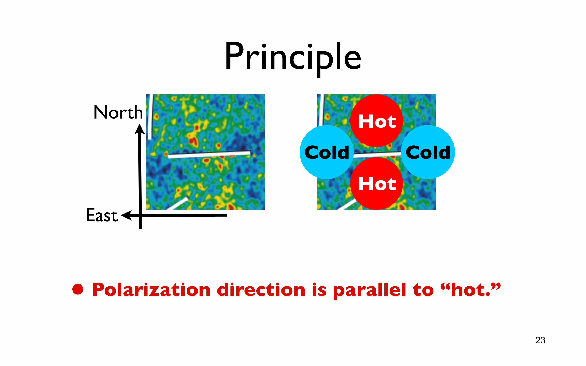
Principle
• Polarization direction is parallel to “hot.”
23
North
East
Hot
Hot
Cold Cold

Two Polarization States of GW
• This is great - this will automatically generate quadrupolar temperature anisotropy around electrons!
24
“+” Mode “X” Mode

From GW to CMB Polarization
Electron
25

From GW to CMB PolarizationRedshift
Redshift
Blue
shift
Blue
shift
Redshift
RedshiftBlu
eshif
tBlues
hift
26

From GW to CMB Polarization
27

“Tensor-to-scalar Ratio,” r
ζIn terms of the slow-roll parameter:
r=16εwhere ε = –(dH/dt)/H2 = 4πG(dφ/dt)2/H2 ≈ (16πG)–1(dV/dφ)2/V2
28

• No detection of polarization from gravitational waves (B-mode polarization) yet.
Pola
riza
tion
Pow
er S
pect
rum
29
from ζ
from h

E-modes
B-modes
30

Proof: A Punch Line
• Detection of the primordial gravitational wave (i.e., the tensor-to-scalar ratio, “r”) with the expected shape of the spectrum provides an ambiguous proof that inflation did occur in the early universe!
31

How can we falsify inflation?
32

How can we falsify single-field inflation?
33

Single Field = Adiabatic fluctuations
• Single-field inflation = One degree of freedom.
• Matter and radiation fluctuations originate from a single source.
= 0
* A factor of 3/4 comes from the fact that, in thermal equilibrium, ρc~(1+z)3 and ργ~(1+z)4.
Cold Dark Matter
Photon
34

35

Non-adiabatic Fluctuations
• Detection of non-adiabatic fluctuations immediately rule out single-field inflation models.
The data are consistent with adiabatic fluctuations:
< 0.09 (95% CL)| |
Komatsu et al. (2011)
36

Inflation looks good(in 2-point function)
• Joint constraint on the primordial tilt, ns, and the tensor-to-scalar ratio, r.
• r < 0.24 (95%CL; WMAP7+BAO+H0)
37

Bispectrum
• Three-point function!
• Bζ(k1,k2,k3) = <ζk1ζk2ζk3> = (amplitude) x (2π)3δ(k1+k2+k3)b(k1,k2,k3)
38
model-dependent function
k1
k2
k3

Single Field Theorem
= Negligible “Local-form” Three-point Function

MOST IMPORTANT

Gaussian? WMAP5
41

Take One-point Distribution Function
•The one-point distribution of WMAP map looks pretty Gaussian.–Left to right: Q (41GHz), V (61GHz), W (94GHz).
•Deviation from Gaussianity is small, if any.42
Spergel et al. (2008)

Inflation Likes This Result
• According to inflation (Mukhanov & Chibisov; Guth & Yi; Hawking; Starobinsky; Bardeen, Steinhardt & Turner), CMB anisotropy was created from quantum fluctuations of a scalar field in Bunch-Davies vacuum during inflation
• Successful inflation (with the expansion factor more than e60) demands the scalar field be almost interaction-free
• The wave function of free fields in the ground state is a Gaussian!
43

But, Not Exactly Gaussian
• Of course, there are always corrections to the simplest statement like this.
• For one, inflaton field does have interactions. They are simply weak – they are suppressed by the so-called slow-roll parameter, ε~O(0.01), relative to the free-field action.
44

A Non-linear Correction to Temperature Anisotropy• The CMB temperature anisotropy, ΔT/T, is given by the
curvature perturbation in the matter-dominated era, Φ.
• One large scales (the Sachs-Wolfe limit), ΔT/T=–Φ/3.
• Add a non-linear correction to Φ:
• Φ(x) = Φg(x) + fNL[Φg(x)]2 (Komatsu & Spergel 2001)
• fNL was predicted to be small (~0.01) for slow-roll models (Salopek & Bond 1990; Gangui et al. 1994)
45
For the Schwarzschild metric, Φ=+GM/R.

fNL: Form of Bζ• Φ is related to the primordial curvature
perturbation, ζ, as Φ=(3/5)ζ.
• ζ(x) = ζg(x) + (3/5)fNL[ζg(x)]2
• Bζ(k1,k2,k3)=(6/5)fNL x (2π)3δ(k1+k2+k3) x [Pζ(k1)Pζ(k2) + Pζ(k2)Pζ(k3) + Pζ(k3)Pζ(k1)]
46

fNL: Shape of Triangle• For a scale-invariant spectrum, Pζ(k)=A/k3,
• Bζ(k1,k2,k3)=(6A2/5)fNL x (2π)3δ(k1+k2+k3) x [1/(k1k2)3 + 1/(k2k3)3 + 1/(k3k1)3]
• Let’s order ki such that k3≤k2≤k1. For a given k1, one finds the largest bispectrum when the smallest k, i.e., k3, is very small.
• Bζ(k1,k2,k3) peaks when k3 << k2~k1
• Therefore, the shape of fNL bispectrum is the squeezed triangle!
47(Babich et al. 2004)

Bζ in the Squeezed Limit
• In the squeezed limit, the fNL bispectrum becomes: Bζ(k1,k2,k3) ≈ (12/5)fNL x (2π)3δ(k1+k2+k3) x Pζ(k1)Pζ(k3)
48

Single-field Theorem (Consistency Relation)
• For ANY single-field models*, the bispectrum in the squeezed limit is given by
• Bζ(k1,k2,k3) ≈ (1–ns) x (2π)3δ(k1+k2+k3) x Pζ(k1)Pζ(k3)
• Therefore, all single-field models predict fNL≈(5/12)(1–ns).
• With the current limit ns=0.96, fNL is predicted to be 0.017.
Maldacena (2003); Seery & Lidsey (2005); Creminelli & Zaldarriaga (2004)
* for which the single field is solely responsible for driving inflation and generating observed fluctuations. 49

Understanding the Theorem
• First, the squeezed triangle correlates one very long-wavelength mode, kL (=k3), to two shorter wavelength modes, kS (=k1≈k2):
• <ζk1ζk2ζk3> ≈ <(ζkS)2ζkL>
• Then, the question is: “why should (ζkS)2 ever care about ζkL?”
• The theorem says, “it doesn’t care, if ζk is exactly scale invariant.”
50

ζkL rescales coordinates
• The long-wavelength curvature perturbation rescales the spatial coordinates (or changes the expansion factor) within a given Hubble patch:
• ds2=–dt2+[a(t)]2e2ζ(dx)2
ζkLleft the horizon already
Separated by more than H-1
x1=x0eζ1 x2=x0eζ2
51

ζkL rescales coordinates
• Now, let’s put small-scale perturbations in.
• Q. How would the conformal rescaling of coordinates change the amplitude of the small-scale perturbation?
ζkLleft the horizon already
Separated by more than H-1
x1=x0eζ1 x2=x0eζ2
(ζkS1)2 (ζkS2)2
52

ζkL rescales coordinates
• Q. How would the conformal rescaling of coordinates change the amplitude of the small-scale perturbation?
• A. No change, if ζk is scale-invariant. In this case, no correlation between ζkL and (ζkS)2 would arise.
ζkLleft the horizon already
Separated by more than H-1
x1=x0eζ1 x2=x0eζ2
(ζkS1)2 (ζkS2)2
53

Real-space Proof• The 2-point correlation function of short-wavelength
modes, ξ=<ζS(x)ζS(y)>, within a given Hubble patch can be written in terms of its vacuum expectation value (in the absence of ζL), ξ0, as:
• ξζL ≈ ξ0(|x–y|) + ζL [dξ0(|x–y|)/dζL]
• ξζL ≈ ξ0(|x–y|) + ζL [dξ0(|x–y|)/dln|x–y|]
• ξζL ≈ ξ0(|x–y|) + ζL (1–ns)ξ0(|x–y|)
Creminelli & Zaldarriaga (2004); Cheung et al. (2008)
3-pt func. = <(ζS)2ζL> = <ξζLζL>= (1–ns)ξ0(|x–y|)<ζL2>
• ζS(x)
• ζS(y)
54

Where was “Single-field”?
• Where did we assume “single-field” in the proof?
• For this proof to work, it is crucial that there is only one dynamical degree of freedom, i.e., it is only ζL that modifies the amplitude of short-wavelength modes, and nothing else modifies it.
• Also, ζ must be constant outside of the horizon (otherwise anything can happen afterwards). This is also the case for single-field inflation models.
55

Probing Inflation (3-point Function)
• No detection of this form of 3-point function of primordial curvature perturbations. The 95% CL limit is:
• –10 < fNLlocal < 74
• fNLlocal = 32 ± 21 (68% CL)
56

WMAP taught us:
• All of the basic predictions of single-field and slow-roll inflation models are consistent with the data (1–ns≈r≈fNL)
• But, not all models are consistent (i.e., λφ4 is out unless you introduce a non-minimal coupling)
57
After 9 years of observations...

However
• We cannot say, just yet, that we have definite evidence for inflation.
• Can we ever prove, or disprove, inflation?
58

Planck may:
• Prove inflation by detecting the effect of primordial gravitational waves on polarization of the cosmic microwave background (i.e., detection of r)
• Rule out single-field inflation by detecting a particular form of the 3-point function called the “local form” (i.e., detection of fNLlocal)
• Challenge the inflation paradigm by detecting a violation of inequality that should be satisfied between the local-form 3-point and 4-point functions
59

Planck might find gravitational waves (if r~0.1)
Planck?
If found, this would give us a pretty
convincing proof that inflation did indeed happen.
60

But...
• Can you falsify inflation (not just single-field models)?
61

Maybe!
• Using the consistency relation between the local-form 3- and 4-point functions.
• Sugiyama, Komatsu & Futamase, PRL, 106, 251301(2011)
• Generalization of the “Suyama-Yamaguchi inequality” (2008)

Which Local-form Trispectrum?• The local-form bispectrum:
• Βζ(k1,k2,k3)=(2π)3δ(k1+k2+k3)fNL[(6/5)Pζ(k1)Pζ(k2)+cyc.]
• can be produced by a curvature perturbation in position space in the form of:
• ζ(x)=ζg(x) + (3/5)fNL[ζg(x)]2
• This can be extended to higher-order:
• ζ(x)=ζg(x) + (3/5)fNL[ζg(x)]2 + (9/25)gNL[ζg(x)]3
63This term (ζ3) is too small to see, so I
will ignore this in this talk.

Two Local-form Shapes• For ζ(x)=ζg(x) + (3/5)fNL[ζg(x)]2 + (9/25)gNL[ζg(x)]3, we
obtain the trispectrum:
• Tζ(k1,k2,k3,k4)=(2π)3δ(k1+k2+k3+k4) {gNL[(54/25)Pζ(k1)Pζ(k2)Pζ(k3)+cyc.] +(fNL)2[(18/25)Pζ(k1)Pζ(k2)(Pζ(|k1+k3|)+Pζ(|k1+k4|))+cyc.]}
k3
k4
k2
k1
gNL
k2
k1
k3
k4
fNL2 64

Generalized Trispectrum
• Tζ(k1,k2,k3,k4)=(2π)3δ(k1+k2+k3+k4) {gNL[(54/25)Pζ(k1)Pζ(k2)Pζ(k3)+cyc.] +τNL[Pζ(k1)Pζ(k2)(Pζ(|k1+k3|)+Pζ(|k1+k4|))+cyc.]}
k3
k4
k2
k1
gNL
k2
k1
k3
k4
τNL 65
The single-source local form consistency relation, τNL=(6/5)(fNL)2, may not be respected –
additional test of multi-field inflation!

(Slightly) Generalized Trispectrum
• Tζ(k1,k2,k3,k4)=(2π)3δ(k1+k2+k3+k4) {gNL[(54/25)Pζ(k1)Pζ(k2)Pζ(k3)+cyc.] +τNL[Pζ(k1)Pζ(k2)(Pζ(|k1+k3|)+Pζ(|k1+k4|))+cyc.]}
k3
k4
k2
k1
gNL
k2
k1
k3
k4
τNL 66
The single-source local form consistency relation, τNL=(6/5)(fNL)2, may not be respected –
additional test of multi-field inflation!

τNL >~ (6fNL/5)2
• The current limits from WMAP 7-year are consistent with single-field or multi-field models.
• So, let’s play around with the future.
67ln(fNL)
ln(τNL)
74
3.3x10⁴
(Smidt et al. 2010)
(Komatsu et al. 2011)
4-point amplitude
3-point amplitude
4-point amplitude
(Suyama & Yamaguchi 2008; Komatsu 2010; Sugiyama, Komatsu & Futamase 2011)

Case A: Single-field Happiness
• No detection of anything (fNL or τNL) after Planck. Single-field survived the test (for the moment: the future galaxy surveys can improve the limits by a factor of ten).
ln(fNL)
ln(τNL)
10
600
68

Case B: Multi-field Happiness(?)
• fNL is detected. Single-field is gone.
• But, τNL is also detected, in accordance with τNL>0.5(6fNL/5)2 expected from most multi-field models.
ln(fNL)
ln(τNL)
600
6930
(Suyama & Yamaguchi 2008; Komatsu 2010; Sugiyama, Komatsu & Futamase 2011)

Case C: Madness• fNL is detected. Single-
field is gone.
• But, τNL is not detected, or found to be negative, inconsistent with τNL>0.5(6fNL/5)2.
• Single-field AND most of multi-field models are gone.
ln(fNL)
ln(τNL)
30
600
70
(Suyama & Yamaguchi 2008; Komatsu 2010; Sugiyama, Komatsu & Futamase 2011)

Cosmology in the Next Decade
• Inflation, Dark Energy, Dark Matter, and Neutrinos...
• We may be able to prove or falsify inflation.
• This has been regarded as impossible in the past, but we may be able to do that!
• Did not have time to talk about: the role of large-scale structure of the Universe on this business, and how we explore DE, DM, and neutrinos...
71

The δN Formalism
• The δN formalism (Starobinsky 1982; Salopek & Bond 1990; Sasaki & Stewart 1996) states that the curvature perturbation is equal to the difference in N=lna.
• ζ=δN=N2–N1
• where N=∫Hdt
Separated by more than H-1
72
Expanded by N1=lna1
Expanded by N2=lna2

Getting the familiar result
• Single-field example at the linear order:
• ζ = δ{∫Hdt} = δ{∫(H/φ’)dφ}≈(H/φ’)δφ• Mukhanov & Chibisov; Guth & Pi; Hawking;
Starobinsky; Bardeen, Steinhardt & Turner
73

Extending to non-linear, multi-field cases
• Calculating the bispectrum is then straightforward. Schematically:
• <ζ3>=<(1st)x(1st)x(2nd)>~<δφ4>≠0
• fNL~<ζ3>/<ζ2>2
(Lyth & Rodriguez 2005)
74

• Calculating the trispectrum is also straightforward. Schematically:
• <ζ4>=<(1st)2(2nd)2>~<δφ6>≠0
• fNL~<ζ4>/<ζ2>3
(Lyth & Rodriguez 2005)
75
Extending to non-linear, multi-field cases

Now, stare at these.
76

Change the variable...
(6/5)fNL=∑IaIbI
τNL=(∑IaI)2(∑IbI)277

Then apply the Cauchy-Schwarz Inequality
• Implies
How generic is this inequality?
(Suyama & Yamaguchi 2008)
78