COST 723 Training School - Cargese 4 - 14 October 2005 OBS 2 Radiative transfer for thermal radiation. Observations Bruno Carli

COST 723 Training School - Cargese 4 - 14 October 2005

OBS 2Radiative transfer for thermal radiation.

Observations

Bruno Carli


Table of Contents• Geometry of observation: zenith, nadir and limb sounding.

• Thermal radiation and types of measurements.

• Spectroscopy.

• The forward model for thermal radiation.

• The inverse problem of atmospheric constituent retrieval.

• Definition of variance-covariance matrix and of averaging kernel matrix.


Geometry of observation

• Zenith sounding

• Nadir sounding

• Limb sounding


Geometry of observationLimb sounding


The vertical and horizontal resolution depend on the geometry of observation.

Typical resolution of nadir measurements is 10 km horizontal and 10 km vertical. Typical resolution of limb measurement is 2 km vertical and 700 km horizontal.

Geometry of observation


Thermal radiation

Thermal radiation

JsTBIs

dx

dI )(

Sun/StarMoon

Earth/planet Atmosphere

SunEarth/atmosphere


Thermal radiation

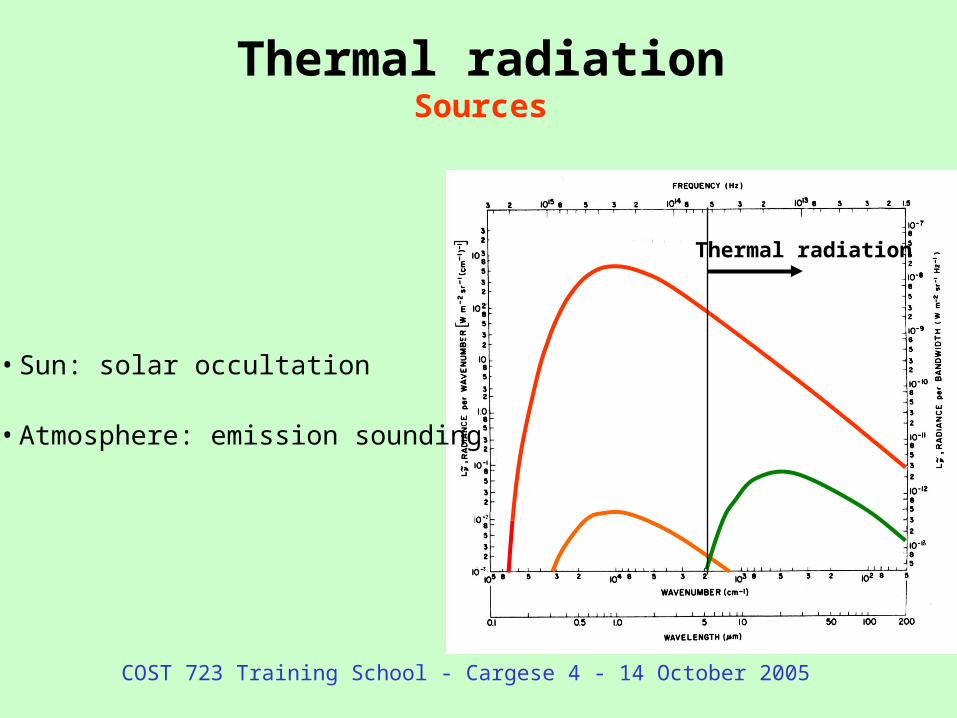
Thermal radiationSources

• Sun: solar occultation

• Atmosphere: emission sounding


Spectroscopy

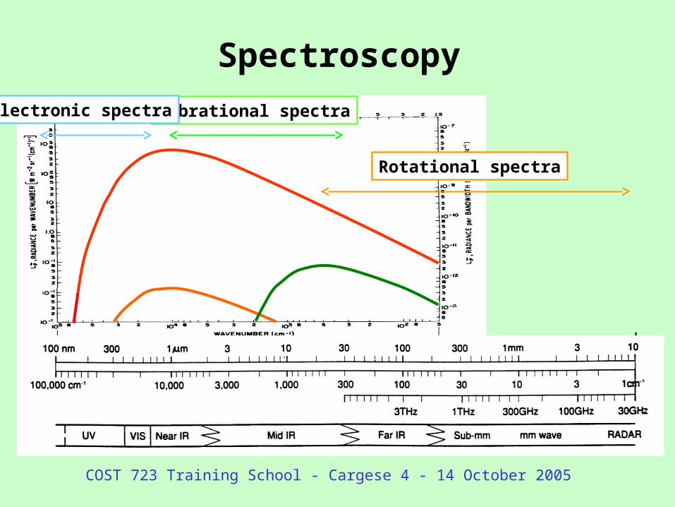
Rotational spectra

Vibrational spectraElectronic spectra


Spectroscopy

Main spectroscopic constituents for the atmosphere:

• water vapor ()

• ozone ()

• carbon dioxide ()

• methane ()

• nitrous oxide ()

• nitric acid ()

Rotational spectra

Vibrational spectra


Spectroscopy

Wavenumber cm-1

Alt

itu

de

km

40

10

30

80

100

90

70

60

50

20

40

10

30

80

100

90

70

60

50

20

110100100010000

Temperature broadening:Gaussian line shape

Pressure broadening:Lorentzian line shape

T

P

Voight line shape equal convolution between Gaussian and Lorentzian distributions.


Integral equation of Radiative TransferIntegral equation of Radiative Transfer

),0(

0),(),0( )()0()(

L LxL dexTBeILI

Absorption term Emission term

Intensity of the background source

“Transmittance”between 0 and L

Spectral intensity observed at L

“Transmittance”between l and L

“Optical depth” L

xdxxLx ')'(),(


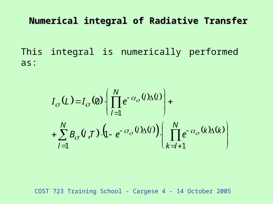
Numerical integral of Radiative TransferNumerical integral of Radiative Transfer

N

l

N

lk

kkll

N

l

ll

eeTlB

eILI

1 1

1

1,

0

This integral is numerically performed as:


Tree of operations for Radiative Transfer calculationTree of operations for Radiative Transfer calculationsegmentationsegmentation


N

l

N

lk

kkllN

l

ll eeTlBeILI1 11

1,0

The optical path is divided in a set of contiguous segments in which the path is straight and the atmosphere has constant properties (segmentation).

In each segment the absorption coefficient is also calculated.

Segments of the optical path 1 ll xxl


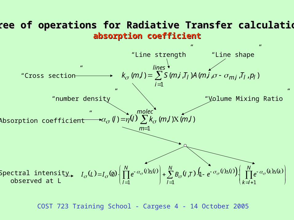
Tree of operations for Radiative Transfer calculationTree of operations for Radiative Transfer calculationabsorption coefficientabsorption coefficient


“Absorption coefficient”

molec

m

lmlmkll1

),(),()(

“number density”

“Cross section”

“Volume Mixing Ratio”

lines

illiml pTimATimSlmk

1, ),,,,(),,(),(

“Line shape”“Line strength”

N

l

N

lk

kkllN

l

ll eeTlBeILI1 11

1,0


The forward model calculates the spectrum measured by the

instrument.

This is equal to the atmospheric spectral intensity I, (L), obtained

with the radiative transfer model, convoluted with instrument effects.

LIIL ,,

Forward Model of the measurementsForward Model of the measurements

Where AILS is the “apodized instrument line shape” and FOV is the

“field of view “ of the instrument.

'''',, dFOVdAILSIS LL


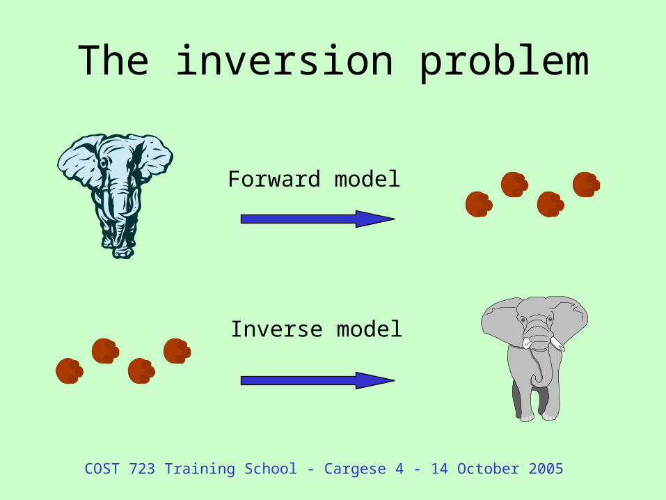
The inversion problem

Forward model

Inverse model


The forward and the inverse problem

The measured signal is determined for several values of the frequency and of the limb angle :

S( , ) ,

and depends on the properties of the atmosphere that, in the

case of a stratified atmosphere, are only a function of the

altitude z :

S( , ) = F(p(z), T(z), VMRi(z) )

where p(z) is the pressure, T(z) is the temperature and

VMRi(z) is the volume mixing ratio of the atmospheric

species i.



In our case, the relationship :

S( , ) = F(p(z), T(z), VMRi(z))

is the forward problem and its reciprocal

p(z) = F1(S( , ))

T(z) = F2(S( , ))

VMRi(z) = Fi(S( , ))

is the inverse problem.



The inverse problem does not always have a useful solution.

In particular it can be :

• ill posed (either impossible solution or infinite possible solutions). This occurs when either an error is made in the definition of the problem or the observations do not provide the required information.

• ill conditioned (the solution exists but small errors in the observations lead to large errors in the solution). This occurs when the observations contains insufficient information.


The inversion problem

Ill conditioned

Ill posed

?


The mathematics of the retrievalThe inversion

In the forward problem

S(, ) = F(p,T,VMR)

(, )=m are the observation variables that number the observations and (p,T,VMR)=q are the atmospheric variables that become the unknowns in the inverse problem. Using these notations :

Sm = F(q)

In general, this equation cannot be analytically inverted and does not have an exact solution.


The mathematics of the retrievalThe least-squares solution

We can look for a least-squares solution. The least-square solution qr is the value of q which minimises the quantity:

2 = yT (Vy)-1 y where Vy is the variance covariance matrix of the measurements and

y = Sm-F(q)

is the difference between the measurements and the forward model calculated for q.


The mathematics of the retrievalThe Gauss-Newton method

The least-square solution is the solution of equation:

(2)/ q = 0.

This equation can be solved with an iterative procedure that starts from an initial guess qo of the unknown.The Gauss-Newton method assumes that qo is near enough to the solution qr and adopts a linear expansion of the non linear functions.


The mathematics of the retrievalThe Gauss-Newton solution

At each step of the iterative process a new estimate qn is obtained : qn = qn-1+(KT (Vy)-1 K)-1 KT (Vy)-1 (Sm-F(qn-1))

where the quantity K=(F(q))/(q) is the Jacobian of the measurements.

When the convergence criteria are satisfied the iterative process is stopped and qr=qn ..

The variance covariance matrix of the solution is equal to:

Vq = (KT (Vy)-1 K)-1


The mathematics of the retrievalThe Levenberg - Marquardt Method

The iterative process may be unstable (the values retrieved at

each iteration oscillate around the solution).

In order to limit this effect it is useful to introduce a damping in

the variation of the unknown (Lavenberg - Marquardt method).

In this case the solution is equal to:

qr = (KT (Vy)-1 K + I)-1 KT (Vy)-1 (Sm-F(qn-1))

where I is the unit matrix.


In the ideal case of absence of both random and systematic errors in the measurements and in the instrument’s forward model, for each state of the atmosphere the observing system provides a retrieved profile .

Expanding up to the first order about a generic atmospheric state , we obtain:

The quantity:

is called averaging kernel (AK) matrix and it is a function of the state .

Averaging kernels

0x

0 xxx

xxx

0

ˆˆˆ v

vv

x

vx̂

0

ˆ

xx

xA

v

0xvx̂

0x


Averaging kernels

The AK matrix describes how the real state of the atmosphere is distorted by the retrieval process.

This information is important whenever the retrieved quantities are used together with other measurements (data assimilation, data validation).


Averaging kernels

The AKs are the

rows of the AK

matrix and provide

for each retrieved

value the

contribution of the

atmosphere at the

different altitudes.


20

40

60

80

-0.2 0.0 0.2 0.4 0.6

Averaging Kernel

Alti

tud

e [k

m]

Averaging kernelsvariabilityvariability

Ozone, all latitudes (April only)


Final considerations

The inversion problem is characterised by:

• the number of observations

• the number of unknowns

• the VCM of the observations

• the VCM of the retrieved unknowns

• the averaging kernel of the retrieval.

Documents

COST 723 Training School - Cargese 4 - 14 October 2005 OBS 2 Radiative transfer for thermal radiation. Observations Bruno Carli